QUANTIFYING BENEFITS OF COOPERATIVE … BENEFITS OF COOPERATIVE ADAPTIVE CRUISE CONTROL TOWARD...
60
QUANTIFYING BENEFITS OF COOPERATIVE ADAPTIVE CRUISE CONTROL TOWARD SUSTAINABLE TRANSPORTATION SYSTEM Pennsylvania State University University of Maryland University of Virginia Virginia Polytechnic Institute and State University West Virginia University The Pennsylvania State University The Thomas D. Larson Pennsylvania Transportation Institute Transportation Research Building University Park, Pennsylvania 16802-4710 Phone: 814-863-1909 Fax: 814-863-3707 www.pti.psu.edu/mautc
Transcript of QUANTIFYING BENEFITS OF COOPERATIVE … BENEFITS OF COOPERATIVE ADAPTIVE CRUISE CONTROL TOWARD...

QUANTIFYING BENEFITS OF COOPERATIVE ADAPTIVE CRUISE CONTROL TOWARD SUSTAINABLE
TRANSPORTATION SYSTEM
Pennsylvania State University University of Maryland University of Virginia
Virginia Polytechnic Institute and State University West Virginia University
The Pennsylvania State University The Thomas D. Larson Pennsylvania Transportation Institute
Transportation Research Building University Park, Pennsylvania 16802-4710 Phone: 814-863-1909 Fax: 814-863-3707
www.pti.psu.edu/mautc
Final Report
QUANTIFYING BENEFITS OF COOPERATIVE ADAPTIVE CRUISE CONTROL TOWARD SUSTAINABLE TRANSPORTATION SYSTEM
Prepared for:
Virginia Department of Transportation
and
U.S. Department of Transportation
Research and Innovative Technology Administration
Prepared by:
Byungkyu (Brian) Park, Ph.D. Associate Professor
Civil and Environmental Engineering
Kristin Malakorn, EIT Graduate Research Assistant
Joyoung Lee, Ph.D. Research Associate
Center for Transportation Studies
University of Virginia
May 2011
This work was sponsored by the Virginia Department of Transportation and the U.S. Department of Transportation, Federal Highway Administration. The contents of this report reflect the views of the authors, who are responsible for the facts and the accuracy of the data presented herein. The contents do not necessarily reflect the official views or policies of either the Federal Highway Administration, U.S. Department of Transportation, or the Commonwealth of Virginia at the time of publication. This report does not constitute a standard, specification, or regulation.
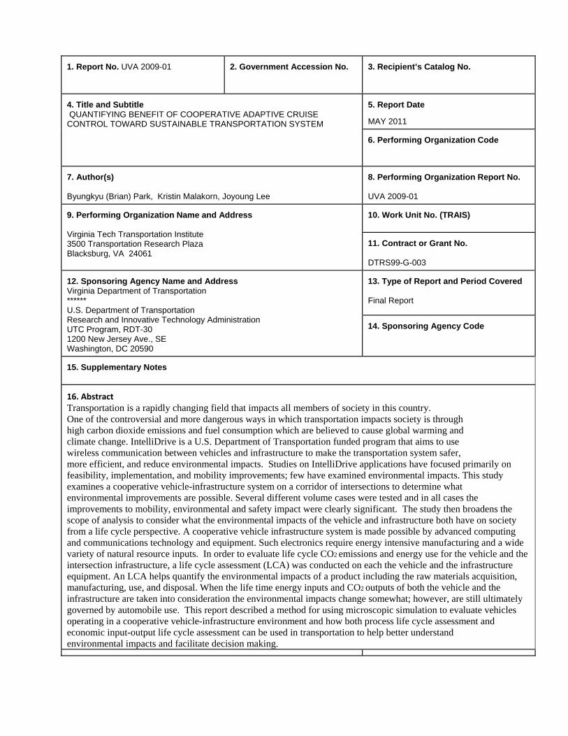
1. Report No. UVA 2009-01
2. Government Accession No.
3. Recipient’s Catalog No.
4. Title and Subtitle QUANTIFYING BENEFIT OF COOPERATIVE ADAPTIVE CRUISE CONTROL TOWARD SUSTAINABLE TRANSPORTATION SYSTEM
5. Report Date
MAY 2011
6. Performing Organization Code
7. Author(s) Byungkyu (Brian) Park, Kristin Malakorn, Joyoung Lee
8. Performing Organization Report No. UVA 2009-01
9. Performing Organization Name and Address Virginia Tech Transportation Institute 3500 Transportation Research Plaza Blacksburg, VA 24061
10. Work Unit No. (TRAIS)
11. Contract or Grant No. DTRS99-G-003
12. Sponsoring Agency Name and Address Virginia Department of Transportation ****** U.S. Department of Transportation Research and Innovative Technology Administration UTC Program, RDT-30 1200 New Jersey Ave., SE Washington, DC 20590
13. Type of Report and Period Covered Final Report
14. Sponsoring Agency Code
15. Supplementary Notes 16. Abstract Transportation is a rapidly changing field that impacts all members of society in this country. One of the controversial and more dangerous ways in which transportation impacts society is through high carbon dioxide emissions and fuel consumption which are believed to cause global warming and climate change. IntelliDrive is a U.S. Department of Transportation funded program that aims to use wireless communication between vehicles and infrastructure to make the transportation system safer, more efficient, and reduce environmental impacts. Studies on IntelliDrive applications have focused primarily on feasibility, implementation, and mobility improvements; few have examined environmental impacts. This study examines a cooperative vehicle-infrastructure system on a corridor of intersections to determine what environmental improvements are possible. Several different volume cases were tested and in all cases the improvements to mobility, environmental and safety impact were clearly significant. The study then broadens the scope of analysis to consider what the environmental impacts of the vehicle and infrastructure both have on society from a life cycle perspective. A cooperative vehicle infrastructure system is made possible by advanced computing and communications technology and equipment. Such electronics require energy intensive manufacturing and a wide variety of natural resource inputs. In order to evaluate life cycle CO2 emissions and energy use for the vehicle and the intersection infrastructure, a life cycle assessment (LCA) was conducted on each the vehicle and the infrastructure equipment. An LCA helps quantify the environmental impacts of a product including the raw materials acquisition, manufacturing, use, and disposal. When the life time energy inputs and CO2 outputs of both the vehicle and the infrastructure are taken into consideration the environmental impacts change somewhat; however, are still ultimately governed by automobile use. This report described a method for using microscopic simulation to evaluate vehicles operating in a cooperative vehicle-infrastructure environment and how both process life cycle assessment and economic input-output life cycle assessment can be used in transportation to help better understand environmental impacts and facilitate decision making.
17. Key Words Intelli-Drive, safer driver, environmental impacts
18. Distribution StatementNo restrictions. This document is available from the National Technical Information Service, Springfield, VA 22161
19. Security Classif. (of this report) Unclassified
20. Security Classif. (of this page) Unclassified
21. No. of Pages 50
22. Price
Technical Report Documentation Page Form DOT F 1700.7 (8-72) Reproduction of completed page authorized

2
i
ABSTRACT
Transportation is a rapidly changing field that impacts all members of society in this country. One of the controversial and more dangerous ways in which transportation impacts society is through high carbon dioxide emissions and fuel consumption which are believed to cause global warming and climate change. IntelliDrive is a U.S. Department of Transportation funded program that aims to use wireless communication between vehicles and infrastructure to make the transportation system safer, more efficient, and reduce environmental impacts.
Studies on IntelliDrive applications have focused primarily on feasibility, implementation, and mobility improvements; few have examined environmental impacts. This study examines a cooperative vehicle-infrastructure system on a corridor of intersections to determine what environmental improvements are possible. Several different volume cases were tested and in all cases the improvements to mobility, environmental and safety impact were clearly significant.
The study then broadens the scope of analysis to consider what the environmental impacts of the vehicle and infrastructure both have on society from a life cycle perspective. A cooperative vehicle-infrastructure system is made possible by advanced computing and communications technology and equipment. Such electronics require energy intensive manufacturing and a wide variety of natural resource inputs.
In order to evaluate life cycle CO2 emissions and energy use for the vehicle and the intersection infrastructure, a life cycle assessment (LCA) was conducted on each the vehicle and the infrastructure equipment. An LCA helps quantify the environmental impacts of a product including the raw materials acquisition, manufacturing, use, and disposal. When the life time energy inputs and CO2 outputs of both the vehicle and the infrastructure are taken into consideration the environmental impacts change somewhat; however, are still ultimately governed by automobile use.
This report described a method for using microscopic simulation to evaluate vehicles operating in a cooperative vehicle-infrastructure environment and how both process life cycle assessment and economic input-output life cycle assessment can be used in transportation to help better understand environmental impacts and facilitate decision making.
ii
Table of Contents Chapter 1. Introduction ...............................................................................................................1
1.1. Motivation .......................................................................................................................1
1.2 Goal..................................................................................................................................2
Chapter 2. Literature Review ......................................................................................................3
2.1 Traffic Signal Control .......................................................................................................3
2.2 Cruise Control Systems.....................................................................................................4
2.2.1 Adaptive Cruise Control.............................................................................................5
2.2.2 Cooperative Adaptive Cruise Control .........................................................................5
2.3 LCA Basics.......................................................................................................................8
2.3.1. ISO LCA Procedure..................................................................................................9
2.3.2. LCA Methods and Tools ......................................................................................... 11
2.4 Life Cycle Assessment in Transportation......................................................................... 13
2.5 Summary ........................................................................................................................ 14
Chapter 3. Methodology............................................................................................................ 16
3.1. Microscopic Traffic Simulation for CVIS-based Control ................................................ 16
3.2 Safety Impact Assessment............................................................................................... 19
3.3. Comparative Life Cycle Assessment .............................................................................. 20
3.3.1 Process LCA Exercise: Traffic Signal Light Bulbs ................................................... 20
3.3.2. Goal and Scope....................................................................................................... 28
3.3.3. Inventory Analysis:................................................................................................. 28
3.3.4. Impact Assessment.................................................................................................. 30
3.4 Automobile Use as Stage of LCA.................................................................................... 30
Chapter 4. Results..................................................................................................................... 32
4.1. Microscopic Traffic Simulation...................................................................................... 32
4.2. Comparative Life Cycle Assessment .............................................................................. 36
4.3. Automobile Use as Stage of LCA................................................................................... 38
Chapter 5. Discussion ............................................................................................................... 41
5.1. CVIS-based Control....................................................................................................... 41
5.2. Comparative Life Cycle Assessment .............................................................................. 43
5.3. Automobile Use as Stage of LCA................................................................................... 43
Chapter 6. Conclusion and Recommendations........................................................................... 44
6.1 Conclusions .................................................................................................................... 44
6.2 Recommendations........................................................................................................... 44
References ................................................................................................................................ 46
iii
Appendix.................................................................................................................................. 50
List of Figures
Figure 1 Use of Added Initial to modify minimum green . .......................................................................4
Figure 2 The impact of fuel price on alternative transportation users .......................................................8
Figure 3 Generic Life Cycle ....................................................................................................................9
Figure 4 ISO standard procedure for performing a LCA ..........................................................................9
Figure 5 Illustration of Vehicle Trajectory Overlap in an intersection ......Error! Bookmark not defined.
Figure 6 SSAM program vehicle interaction ......................................................................................... 19
Figure 7 Conceptual Workflow ............................................................................................................. 20
Figure 8 Halogen Incandescent light bulb product system. .......................................................................1
Figure 9 Light Emitted Diode diagram .................................................................................................. 23
Figure 10 LCA of Halogen Incandescent Light Bulb and LED light bulbs excluding use stage............... 25
Figure 11 LCA of Halogen Incandescent Light bulb and LED light bulbs. ............................................. 26
Figure 12 LCA of Halogen Incandescent light bulb and LED light bulbs normalized to LED lifetime. ... 26
Figure 13 Lifecycle costs of each light bulb over the lifetime of one LED signal face............................. 27
Figure 14 Current Automobile and Intersection Infrastructure EIOLCA results...................................... 37
Figure 15 Cooperative Automobile and Intersection Infrastructure EIOLCA results............................... 37
Figure 16 Cooperative Automobile and Conversion Intersection Infrastructure EIOLCA results ............37
Figure 17 Task 2 summary results ......................................................................................................... 38
Figure 18 Current vehicle and intersection infrastructure life cycle CO2 and energy use ......................... 39
Figure 19 Cooperative vehicle and intersection infrastructure life cycle CO2 and energy use ................. 39
Figure 20 Cooperative vehicle and conversion infrastructure life cycle CO2 and energy use .................. 39
Figure 21 Task 3 summary results ......................................................................................................... 40
Figure 22 CO2 emissions with signal delay ............................................................................................ 42
Figure 23 Fuel consumption with signal delay ....................................................................................... 42
Figure 24 Fuel economy with signal delay............................................................................................. 42
iv
List of Tables
Table 1 Eight Volume Cases tested........................................................................................................ 18
Table 2 Case 1 results and statistical analysis......................................................................................... 32
Table 3 Case 2 results and statistical analysis......................................................................................... 32
Table 4 Case 3 results and statistical analysis......................................................................................... 33
Table 5 Case 4 results and statistical analysis......................................................................................... 33
Table 6 Case 5 results and statistical analysis......................................................................................... 33
Table 7 Case 6 results and statistical analysis......................................................................................... 34
Table 8 Case 7 results and statistical analysis......................................................................................... 34
Table 9 Case 8 results and statistical analysis......................................................................................... 34
Table 10 CVIS control safety improvements......................................................................................... 36

v
Chapter 1. Introduction
Sustainability has emerged as a key issue in transportation. Carbon dioxide and greenhouse gas emissions from the transportation sector are damaging the atmosphere and the environment. This damage is having noticeable ramifications worldwide. Americans have done nothing to change their transportation habits and curb their fuel usage, furthering national dependency on foreign oil.
While the world wrestles with issues of sustainability and greenhouse gas emissions, technology is advancing in the communications, computing, and transportation fields that could transform how the transportation system operates in the United States. IntelliDrive-based vehicle-infrastructure control systems are one application at the center of that transformation. This report examines a cooperative vehicle-infrastructure control system and analyzes it for potential life time impacts on the environment, which are not limited to vehicle fuel usage and miles traveled. This analysis will use microscopic traffic simulation and life cycle assessment to achieve its goals.
This report is organized into six chapters. The remaining sections of chapter 1 describe the motivation and specific goals of this project in terms of three tasks. Chapter 2 is a literature review of the various topics that make up this project, Chapter 3 describes the methodology, Chapter 4 presents the results, Chapter 5 is a discussion of the results, and Chapter 6 summarizes the research, the results found and presents some potential future research that this project has offered.
1.1. Motivation
In 2007 the United States emitted 5,838,381 thousand metric tons of CO2 from human related sources (1). This made up almost 20% of CO2 emissions from human sources worldwide (1). In 2009, the U.S. Environmental Protection Agency released a statement stating that greenhouse gases, specifically carbon dioxide are harmful to the environment and to public health (2). Carbon dioxide, specifically, is cited as being a major factor contributing to climate change (2). Furthermore, this announcement also clearly states that ‘on-road vehicles contribute to this threat’ due to GHG emissions generated by burning gasoline to power vehicles (2). In 2006, the transportation sector was second in CO2 emissions due to human related sources in the United States, preceded only by the electricity sector (3). Within CO2 emissions from transportation, two-thirds of emissions were from non-freight sources, i.e. personal transportation.
Fortunately, the EPA is not the only government agency taking notice of the high CO2 emissions being caused by transportation. IntelliDrive is a U.S. Department of Transportation (DOT) supported program that is focused on improving transportation through vehicle to vehicle and vehicle to infrastructure communication (4). The goals of the IntelliDrive program include improving transportation safety, efficiency, and reducing impacts on the environment through vehicle communication. One area of research that IntelliDrive will be working on has been titled AERIS, Applications for the Environment: Real-time Information Synthesis. The basic objective of AERIS is to understand how the acquisition and use of real-time ITS data can positively influence transportation impacts on the environment (5).
Although this clearly explains the importance of investigating IntelliDrive applications and the role they will play in the future of transportation, it does not address the importance of examining such applications from a life cycle standpoint. Life Cycle Assessment (LCA) is a method for quantifying environmental impacts of a product or process over an entire life cycle. The life cycle begins at raw materials acquisition and ends with the disposal of the product. This is a much broader scope to study a product over than what is typically chosen. This broader scope is a more accurate illustration of environmental impacts than looking solely at the use of a product. The best example of this in transportation is the electric vehicle. The electric vehicle may look like the more environmentally friendly choice if one only considers the impacts of driving an electric vehicle verses driving a gasoline powered vehicle. The electric vehicle has zero tail pipe emissions while the gasoline powered vehicle undoubtedly emits dangerous greenhouse gases and particulate matter into the atmosphere. The obvious
2
choice appears to be the electric vehicle. However, if the scope of the analysis is broadened the obvious choice becomes unclear. The electric vehicle is powered by electricity which, the majority of the time, is produced by burning coal. This results in high greenhouse gas and particulate matter emissions as well. In 2006, the electricity sector was first in CO2 emissions by human sources in the United States (3). Another factor impacting the environmental friendliness of electric vehicles is in the battery production. Some processes associated with battery manufacture for an electric vehicle and gasoline powered vehicles are different and could alter the environmental impacts of the vehicle as a whole.
One manufacturing issue of particular interest for this study is the impact of manufacturing electronic parts and semiconductors that would be necessary for extensive communication and vehicle control equipment. The belief that manufacturing semiconductors and other electronic parts are a burden on the environment is best described by Eric Williams (6). If every vehicle in the United States and every signalized intersection required new, additional electronics in order to operate in the cooperative transportation system then that may change how transportation is impacting the environment.
1.2 Goal
The goal of this research is to examine an IntelliDrive based cooperative vehicle-infrastructure control system as an alternative to current transportation infrastructure, and determine the better option from an environmental perspective. Transportation is heavily associated with greenhouse gas emissions and global warming, therefore, the better option would be the one that results in lower CO2 emissions and fuel consumption.
This goal will be achieved through the following tasks:
1. Determination of the benefits of IntelliDrive based cooperative vehicle-infrastructure control systems in terms of mobility and environmental impact.
2. Comparative Life Cycle Assessment of cooperative and traditional transportation infrastructure systems including both vehicles and infrastructure.
3. Integration of Task 1 results into Task 2, Life Cycle Assessment results. To determine whether additional cooperative equipment impacts can be offset by savings in fuel from improved fuel economy.
3
1.
Chapter 2. Literature Review
The cooperative vehicle-infrastructure control system that has been described could be made possible using an IntelliDrive application, Cooperative Adaptive Cruise Control (CACC). For that reason, the focus of the literature review will be on CACC research and innovations, and examples of how CACC can be used in communication with traffic signals to improve the quality of transportation. This chapter is divided into five sections describing the research in the following areas: traffic signal control, cruise control systems, life cycle assessment, life cycle assessment applications in transportation, and finally a summary of the literatures reviewed.
2.1 Traffic Signal Control
Traffic signals have been around since the mid-1800s (7). Over the last 150 years there have been major innovations in how traffic signals are controlled and the methods behind deciding when vehicles can get the green light. The original traffic signal was controlled by a police officer standing at the intersection using their best judgment to move vehicles throughout a city. The police officer’s job was made easier by constructing a traffic tower which the officer could stand on to increase their visibility of the roads and allow them to better manage traffic (7).
In the 1920s these towers began to hold 4-way 3-color signals, which were eventually pretimed; traffic control was no longer responsive to traffic conditions. However, in 1928 the first horn actuated signal was installed in Baltimore, MD (7). This is one of the first attempted to make traffic signals responsive to traffic without the presence of a person to tell the signal when to change. This was followed by other inventions that used sound waves to alert a traffic signal about the presences of a vehicle. From this point to the present, vehicle presence at an intersection is the only way for a vehicle to communicate to the traffic signal that they would like to proceed through an intersection. Devices that allow for this today include inductive loops which use a magnetic field to detect vehicles, or video detection which can detect important changes in a video image to detect vehicle presence at a signal. The most common way to predict, rather than detect, a vehicle at an intersection would be to install inductive loops on the roadway some distance prior to an intersection.
Although traffic signals cannot solve all traffic problems, using traffic signals does have some benefits (8):
1. Provide for the orderly and efficient movement of people 2. Effectively maximize the volume movements served at the intersection 3. Reduce the frequency and severity of certain types of crashes 4. Provide appropriate levels of accessibility for pedestrians and side street traffic.
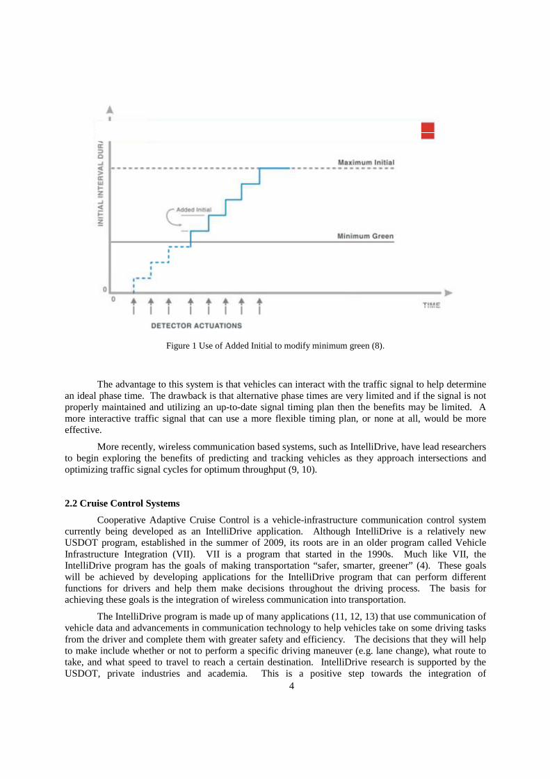
Actuated traffic signals make up the majority of traffic signals used today in the United States. These signals are an improvement on pre-timed traffic signals because the signal timing at an actuated signal can change from one phase to the next. This allows approaches with higher traffic volumes to receive more green time than other approaches with lower volumes. The way that signals do this is each signal phase has a minimum and a maximum allowable green time. All phases will initially provide the minimum green time, however it can be extended as vehicles approaching the intersection are detected. A reasonable vehicle extension time is about 3 seconds for an approaching vehicle, but should be adjusted so that it is appropriate for the vehicle placing the call to travel from the detector to the stop bar and safely cross the intersection. Vehicles can continue to place calls resulting in extensions until the maximum green time is reached. Figure 1 illustrates this concept.
4
Figure 1 Use of Added Initial to modify minimum green (8).
The advantage to this system is that vehicles can interact with the traffic signal to help determine an ideal phase time. The drawback is that alternative phase times are very limited and if the signal is not properly maintained and utilizing an up-to-date signal timing plan then the benefits may be limited. A more interactive traffic signal that can use a more flexible timing plan, or none at all, would be more effective.
More recently, wireless communication based systems, such as IntelliDrive, have lead researchers to begin exploring the benefits of predicting and tracking vehicles as they approach intersections and optimizing traffic signal cycles for optimum throughput (9, 10).
2.2 Cruise Control Systems
Cooperative Adaptive Cruise Control is a vehicle-infrastructure communication control system currently being developed as an IntelliDrive application. Although IntelliDrive is a relatively new USDOT program, established in the summer of 2009, its roots are in an older program called Vehicle Infrastructure Integration (VII). VII is a program that started in the 1990s. Much like VII, the IntelliDrive program has the goals of making transportation “safer, smarter, greener” (4). These goals will be achieved by developing applications for the IntelliDrive program that can perform different functions for drivers and help them make decisions throughout the driving process. The basis for achieving these goals is the integration of wireless communication into transportation.
The IntelliDrive program is made up of many applications (11, 12, 13) that use communication of vehicle data and advancements in communication technology to help vehicles take on some driving tasks from the driver and complete them with greater safety and efficiency. The decisions that they will help to make include whether or not to perform a specific driving maneuver (e.g. lane change), what route to take, and what speed to travel to reach a certain destination. IntelliDrive research is supported by the USDOT, private industries and academia. This is a positive step towards the integration of
5
communication into vehicles and infrastructure to improve the quality of everyday driving. The specific IntelliDrive application that will be discussed is Cooperative Adaptive Cruise Control.
Cruise control is an older concept that is familiar to most drivers and is a fairly standard feature on recently purchased vehicles. This simple system is the basis for two newer concepts being developed and researched as a part of the IntelliDrive program. These concepts are Adaptive Cruise Control, ACC, and Cooperative Adaptive Cruise Control, CACC, built off of the ACC system.
2.2.1 Adaptive Cruise Control
Cruise control systems allow drivers to pick a desired highway cruising speed, set their vehicle to move at that speed, and let the vehicle drive. This system assists drivers by taking on the task of powering the vehicle while the driver is still responsible for controlling the direction of the vehicle and being aware of possible dangers in the roadway that require a speed reduction. Adaptive Cruise Control was designed to be safer than traditional cruise control. ACC also allows drivers to set a desired highway cruising speed, and let the vehicle drive from there. The difference between ACC and a traditional cruise control system is that ACC systems have much greater control over the engine and braking system. This allows the ACC system to speed up or slow down the vehicle if needed. The way that a vehicle knows to slow down or speed up is through the use of sensors in the front and rear of the vehicle. The best use for this application is in the case of two vehicles, one following the other. Assuming the vehicle equipped with ACC is a following vehicle, it can detect changes in the space in front of it as the following vehicle approaches the leading vehicle. If the vehicles approach too close to one another the following ACC equipped vehicle can safely slow itself down to avoid a potential collision with the leading vehicle. When the time gap between vehicles has returned to a safe distance the vehicle can return to the desired traveling speed set by the driver. All of these actions are carried out by the vehicle without being initiated by the driver as long as the ACC is set.
The safety improvements that ACC could potentially yield are obvious. By taking responsibility of maintaining a following distance out of the hands of the driver human error can be avoided and collisions, specifically rear end collisions could be avoided. ACC additionally has potential to yield improvements in mobility, particularly in highway settings. Because the automobile has greater control over speed and better reaction time to possible dangers the following gap between vehicles can be reduced. The following gap is the time gap between vehicles measured in seconds. The following gap, like the travel speed, can also be selected by the driver and can range from 1.1-2.2 seconds (14). 3 seconds is considered a safe following time gap for vehicles (15). At gaps of 3 seconds, vehicles are considered to only take up a small percentage of the roadway thus making for very inefficient use of the roadway (16). If the time gap between vehicles can be reduced the capacity of the nation’s highways could be substantially increased, possibly doubled (16).
Adaptive Cruise Control is currently available in new and high end vehicles. As ACC begins to penetrate the market there will certainly be further research and information available on how well it may or may not be performing. Cooperative Adaptive Cruise Control, however, is the next generation of cruise control systems under research and is not yet available on the road.
2.2.2 Cooperative Adaptive Cruise Control
Cooperative Adaptive Cruise Control, CACC, builds further on the ACC and application described. CACC systems are an ACC system with the addition of communication hardware. CACC also controls the vehicle speed with the goal of maintaining the speed set by the driver, and also uses sensors to help detect changes in the gap between lead and following vehicles. The major difference between ACC and CACC systems is CACC uses a wireless communication system to share key vehicle
6
and travel information that is primarily used to make travel speed decisions. Dedicated Short Range Communication, DSRC, is one method for establishing wireless communication and works much like transmitting a radio signal or a Wi-Fi signal from a point out over a range where vehicles can pick it up. DSRC allows for vehicle to vehicle communication and vehicle to infrastructure communication. The vehicle to vehicle communication system allows vehicles to share information about speed, location, acceleration, deceleration, braking pressure, and roadway alerts, just to name a few. Not only does CACC provide more information about each vehicle to others, it also can provide it much sooner. The range of the DSRC as compared to the range of sensors mounted on the front of a vehicle is much greater. That translates into more data at faster speeds. This information can be shared among vehicles to improve following distances and speeds, anticipate dangerous situations or be used to help vehicles form platoons for improved mobility.
Vehicle-infrastructure communication provides further benefits to drivers. Vehicle to infrastructure communication allows any piece of infrastructure equipped with communications hardware to exchange information with the vehicles using the roadway. For example, a communication point along the roadway could inform incoming vehicles that there is an accident and congestion coming up and suggest possible actions to be taken. Another possible use for vehicle to infrastructure communication is at traffic signals; a traffic signal could inform a vehicle about cycle lengths and green times so the vehicle could adjust its traveling speed for the best arrival time.
Just as with ACC, drivers can set the cruising speed and following gap times that are both maintained with CACC. Gap distances for CACC are shorter because of the increased speed and quality of vehicle data that wireless communication allows and can range from 0.6-1.1 seconds (14). The vehicle still operates in the same general manner as the ACC equipped vehicle, however, better informed decisions can be made about route choices, accelerating, or decelerating relative to the previous scenarios. More route options and greater control over vehicle speed opens up opportunities for increased mobility and improvements in fuel consumption and environmental impact. Much of the research in the area of CACC is ongoing as a part the IntelliDrive program and many of the results are preliminary. The following studies begin to show the great impact that CACC technology can have on transportation.
The University of California Berkeley PATH program has done a large volume of research and development work on CACC technology. In a study reported on in 2009, the PATH program developed two vehicles that use CACC technology and ran tests using them to determine how CACC would change driving. The researchers were able to determine that CACC enabled vehicles had faster response times than ACC enabled vehicles when changes to speed need to be made. This improved response time is due to the cooperation between vehicles who are exchanging data, rather than using sensors to collect data at the time it is needed (14). Because vehicles outfitted with CACC technology have faster reaction times to changes by a lead vehicle, the expectation is that safety using this system will improve over the status quo at least as much as use of the ACC system permits, quite possibly more.
The PATH program also addressed the issue of mobility and examined how CACC can improve mobility for vehicles through successful development of a CACC prototype vehicle. This vehicle successfully followed and responded to speed changes in a lead vehicle, just as an ACC vehicle, but with greater precision (14). As noted earlier, vehicles using CACC systems can chose to follow vehicles at time gaps of 0.6-1.1 seconds as compared to the 1.1-2.2 second gaps used in the ACC system. The belief is that the shorter CACC gaps would increase roadway capacity if enough vehicles used the shorter following gaps. Depending on the length of the gap, this could double roadway capacity in some places. Increases in capacity of this magnitude would surely be able to increase mobility on highways (14).
Experiments conducted by the PATH program using a prototype vehicle and 12 subjects show that drivers are comfortable using short driving gaps for low to moderate volume conditions, however, drivers tend not to use the application for congested driving conditions (16).
7
In a 2006 study by van Arem et al., microscopic simulation was used to evaluate mobility improvements made possible with cooperative adaptive cruise control (17). For this study a 4 lane highway that merges to become a 3 lane highway was modeled. The number of shockwaves that formed was counted and used as a measure for evaluating the quality of mobility. This study found that as market penetration rose the number of shockwaves dropped and that generally the average speed of vehicle travel rose (17). Shockwaves are considered a dangerous situation for travelers due to major changes in speed and acceleration. A reduction in the number of shockwaves could be seen as a safety improvement; however, that conclusion was not made because lateral vehicle control is also required for safe lane merging which was not addressed by this study.
Most recently, Lee has used a cooperative vehicle-infrastructure system (CVIS) test-bed to simulate a cooperative vehicle control system that would be representative of cooperative adaptive cruise control (18). This test-bed was made up of an isolated intersection with single lane approaches and departures on all four legs. This study resulted in reductions of stop delay of 99%, travel time improvements of 33%, and carbon dioxide emissions reductions and energy savings of 44% (18). This test-bed is the basis for the simulation work done in this research project. For this project the test-bed was expanded upon to optimized more than a single isolated intersection.
Another study conducted at UC Berkeley attempts to test the vehicle to infrastructure communication capabilities of a CACC system and what the greater benefits of its use could be, specifically environmental impact benefits. The belief is that better speed choices would lead to a smoother ride, improved mobility and possibly reduce fuel consumption. High acceleration and deceleration rates cause increased fuel consumption and CO2 emissions. A simulation study was done on a corridor made up of 10 signalized intersections. The vehicle in this simulation was able to communicate with the upcoming traffic signals and was told what color the light was going to be during their arrival at the stop bar. Given this information, the CACC system could change the vehicle speed to help the vehicle reduce accelerations and decelerations and arrive at the stop bar on a green light. By using CACC to communicate with the traffic signal the vehicle was able to reduce travel times by about 1% (19), suggesting insignificant improvements to mobility. What is impressive about the results is the fuel and emissions savings. Fuel savings using this application were about 12% and carbon dioxide savings about 14%. However, this simulation was conducted for a single vehicle and does not show significant improvements in mobility.
Literature available on cooperative adaptive cruise control is limited to studies on development and feasibility of this technology, driver willingness to use this technology and the possible mobility improvements that could be seen by implementing such a system. Safety is likely not studied in detail because safety is very challenging to assess using simulation for typical conditions, and this technology is not widely available for testing on road. Although environmental impacts and “greener” solutions in transportation is also an IntelliDrive goal, very limited research has been done in this area with the exception of Mandava et al. (19).
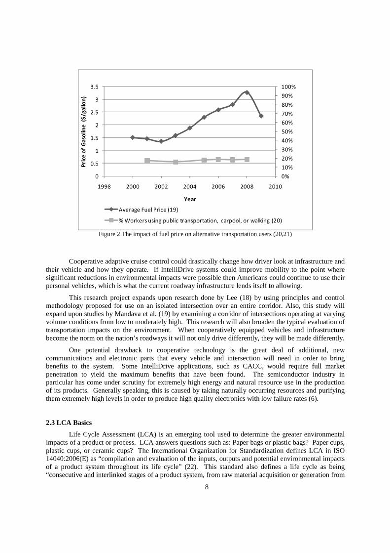
As stated, the transportation sector is responsible for huge vehicle emissions and needs to make changes in order to prevent doing further damage to the environment. The public in this country has not shown an interest in changing their transportation habits. Even during periods when fuel prices sky-rocketed, Americans were not very receptive to public transit options, and in many places they are not available with the connectivity necessary for most commuters. Figure 2 shows that regardless of fuel prices, plotted on the left axis, Americans transportation habits remain unchanged.
8
0%
10%
20%
30%
40%
50%
60%
70%
80%
90%
100%
0
0.5
1
1.5
2
2.5
3
3.5
1998 2000 2002 2004 2006 2008 2010
Pri
ce o
f G
aso
lin
e (
$/
gallo
n)
Year
Average Fuel Price (19)
% Workers using public transportation, carpool, or walking (20)
Figure 2 The impact of fuel price on alternative transportation users (20,21)
Cooperative adaptive cruise control could drastically change how driver look at infrastructure and their vehicle and how they operate. If IntelliDrive systems could improve mobility to the point where significant reductions in environmental impacts were possible then Americans could continue to use their personal vehicles, which is what the current roadway infrastructure lends itself to allowing.
This research project expands upon research done by Lee (18) by using principles and control methodology proposed for use on an isolated intersection over an entire corridor. Also, this study will expand upon studies by Mandava et al. (19) by examining a corridor of intersections operating at varying volume conditions from low to moderately high. This research will also broaden the typical evaluation of transportation impacts on the environment. When cooperatively equipped vehicles and infrastructure become the norm on the nation’s roadways it will not only drive differently, they will be made differently.
One potential drawback to cooperative technology is the great deal of additional, new communications and electronic parts that every vehicle and intersection will need in order to bring benefits to the system. Some IntelliDrive applications, such as CACC, would require full market penetration to yield the maximum benefits that have been found. The semiconductor industry in particular has come under scrutiny for extremely high energy and natural resource use in the production of its products. Generally speaking, this is caused by taking naturally occurring resources and purifying them extremely high levels in order to produce high quality electronics with low failure rates (6).
2.3 LCA Basics
Life Cycle Assessment (LCA) is an emerging tool used to determine the greater environmental impacts of a product or process. LCA answers questions such as: Paper bags or plastic bags? Paper cups, plastic cups, or ceramic cups? The International Organization for Standardization defines LCA in ISO 14040:2006(E) as “compilation and evaluation of the inputs, outputs and potential environmental impacts of a product system throughout its life cycle” (22). This standard also defines a life cycle as being “consecutive and interlinked stages of a product system, from raw material acquisition or generation from
9
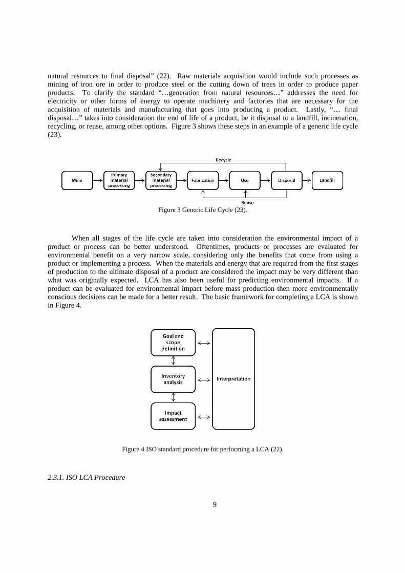
natural resources to final disposal” (22). Raw materials acquisition would include such processes as mining of iron ore in order to produce steel or the cutting down of trees in order to produce paper products. To clarify the standard “…generation from natural resources…” addresses the need for electricity or other forms of energy to operate machinery and factories that are necessary for the acquisition of materials and manufacturing that goes into producing a product. Lastly, “… final disposal…” takes into consideration the end of life of a product, be it disposal to a landfill, incineration, recycling, or reuse, among other options. Figure 3 shows these steps in an example of a generic life cycle (23).
Figure 3 Generic Life Cycle (23).
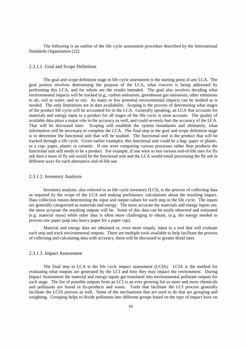
When all stages of the life cycle are taken into consideration the environmental impact of a product or process can be better understood. Oftentimes, products or processes are evaluated for environmental benefit on a very narrow scale, considering only the benefits that come from using a product or implementing a process. When the materials and energy that are required from the first stages of production to the ultimate disposal of a product are considered the impact may be very different than what was originally expected. LCA has also been useful for predicting environmental impacts. If a product can be evaluated for environmental impact before mass production then more environmentally conscious decisions can be made for a better result. The basic framework for completing a LCA is shown in Figure 4.
Figure 4 ISO standard procedure for performing a LCA (22).
2.3.1. ISO LCA Procedure
10
The following is an outline of the life cycle assessment procedure described by the International Standards Organization (22).
2.3.1.1. Goal and Scope Definition
The goal and scope definition stage in life cycle assessment is the starting point of any LCA. The goal portion involves determining the purpose of the LCA, what concern is being addressed by performing this LCA, and for whom are the results intended. The goal also involves deciding what environmental impacts will be tracked (e.g., carbon emissions, greenhouse gas emissions, other emissions to air, soil or water, and so on). As many or few potential environmental impacts can be studied as is needed. The only limitations are in data availability. Scoping is the process of determining what stages of the product life cycle will be accounted for in the LCA. Generally speaking, an LCA that accounts for materials and energy input to a product for all stages of the life cycle is most accurate. The quality of available data plays a major role in the accuracy as well, and could severely hurt the accuracy of the LCA. That will be discussed later. Scoping will establish the system boundaries and ultimately, what information will be necessary to complete the LCA. The final step in the goal and scope definition stage is to determine the functional unit that will be studied. The functional unit is the product that will be tracked through a life cycle. Given earlier examples, this functional unit could be a bag- paper or plastic, or a cup- paper, plastic or ceramic. If one were comparing various processes rather than products the functional unit still needs to be a product. For example, if one were to test various end-of-life uses for fly ash then a mass of fly ash would be the functional unit and the LCA would entail processing the fly ash in different ways for each alternative end-of-life use.
2.3.1.2. Inventory Analysis
Inventory analysis, also referred to as life cycle inventory (LCI), is the process of collecting data as required by the scope of the LCA and making preliminary calculations about the resulting impact. Data collection means determining the input and output values for each step in the life cycle. The inputs are generally categorized as materials and energy. The more accurate the materials and energy inputs are, the more accurate the resulting outputs will be. Some of this data can be easily observed and estimated (e.g. material mass) while other data is often more challenging to obtain, (e.g. the energy needed to process raw paper pulp into heavy paper for a paper cup).
Material and energy data are tabulated or, even more simply, input to a tool that will evaluate each step and track environmental outputs. There are multiple tools available to help facilitate the process of collecting and calculating data with accuracy, these will be discussed in greater detail later.
2.3.1.3. Impact Assessment
The final step in LCA is the life cycle impact assessment (LCIA). LCIA is the method for evaluating what outputs are generated by the LCI and how they may impact the environment. During Impact Assessment the material and energy inputs get translated into environmental pollutant outputs for each stage. The list of possible outputs from an LCI is an ever growing list as more and more chemicals and pollutants are found in by-products and waste. Tools that facilitate the LCI process generally facilitate the LCIA process as well. Some of the mechanisms that are used to do that are grouping and weighting. Grouping helps to divide pollutants into different groups based on the type of impact have on
11
the environment. Pollutants related to global warming are generally grouped together, as are heavy metals, emissions to water, and so on. Weighting is a process of assigning value to pollutants to take a weighted sum of pollutants to more appropriately reflect the impacts to the environment. The process of assessing these various impacts is also not as straightforward as simply adding up toxins. For example, one gram of carbon dioxide (CO2) does not have the same environmental implications as one gram of nitrogen oxides (NOx). This is where a unit such as CO2 equivalent is useful for emissions that are relevant in the area of global warming. Many tools will suggest a weighting scheme that is appropriate for the desired outputs of the LCA.
2.3.1.4. Interpretation
This step in the LCA framework is always present and necessary after every step to ensure that the LCA is meeting the goals established. As the two way arrows in Figure 4 suggest, it is often necessary to revisit prior steps and make changes throughout the LCA process. Interpretation is the step that allows for evaluating and making changes to the developing LCA. There are many instances when one may need to return to a previous step and make changes.
2.3.2. LCA Methods and Tools
Life cycle assessment can be simplified by using software tools available for organizing, collecting, calculating, and analyzing data. Before these useful tools can be explained, the two general methods for conducting an LCA must be understood. The two general methods are process LCA and economic input-output LCA. The former more obviously relates to the LCA framework that has been explained. Economic input-output LCA (EIO LCA) accomplishes the same goal in a way that does not rely on the individual stages of the life cycle shown in Figure 3, rather it requires economic data. Additionally, a third method is to perform a hybrid LCA; which combines the process and EIO methods in an attempt to yield a more accurate result.
2.3.2.1. Process Life Cycle Assessment
The key concepts behind a process LCA have already been described in the Life Cycle Assessment Basics section. To summarize, a process LCA requires mapping the entire life cycle of a product, in detail, including all processes and transportation between life cycle stages, all materials entering the life cycle, all energy inputs to the system, and all outputs. This method is also called the process sum method. The key to this method is determining the outputs to the environment that result from each stage in the life cycle and summing them at the end.
This can quickly become a tedious process. What a software tool will do to facilitate is organize inventory data and help build life cycle stages with visual tools. After data collection, software tools can also help with the calculation of different outputs, grouping, weighting, and analysis such as sensitivity and uncertainty analysis and simple reporting. Such software packages include SimaPro by Product Ecology Consultants, PRé (24), OpenLCA (25), and GaBi software from PE International (26).
What software packages alone lack is data. It can be very challenging to determine with accuracy how much electricity is required for a manufacturing operation, or how much, iron ore is needed to produce a steel beam. There are multiple databases to choose from depending on the goal of an LCA; however, the Ecoinvent database is a well known choice (27). This database of impact information includes a wide range of industry processes, material and energy inputs, and transportation processes.
12
The Ecoinvent database does not contain data for every process possible, but this database will ease much of the data mining typically needed. Another benefit to using this or another database is transparency. Using a database makes an LCA easier for others to follow and trust the result.
One drawback to choosing to do a process LCA is that if there is any missing data or a process is neglected then there are emissions missing from the final result and the resulting impacts are underestimated. Because companies want to maintain their competitive edge they are often reluctant to release information about their processes for widespread analysis. Another drawback has already been suggested, that is the intensive data needs to complete a process LCA. EIO LCA provides some solutions to these problems.
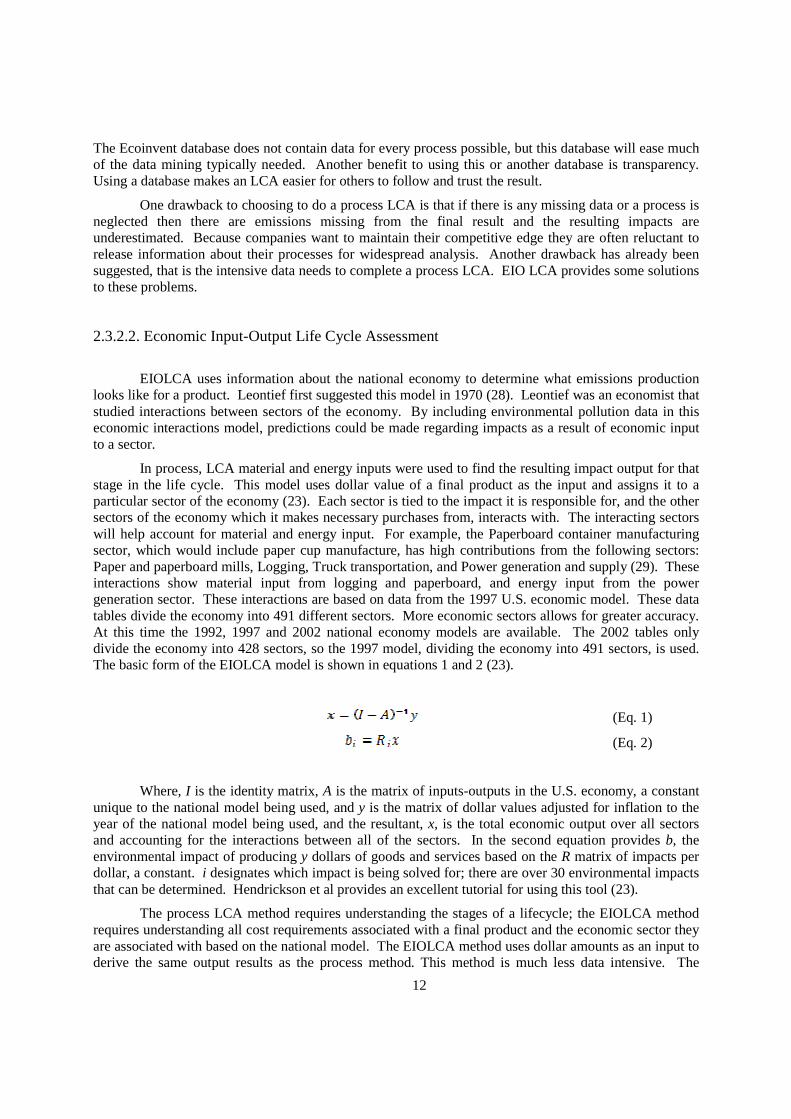
2.3.2.2. Economic Input-Output Life Cycle Assessment
EIOLCA uses information about the national economy to determine what emissions production looks like for a product. Leontief first suggested this model in 1970 (28). Leontief was an economist that studied interactions between sectors of the economy. By including environmental pollution data in this economic interactions model, predictions could be made regarding impacts as a result of economic input to a sector.
In process, LCA material and energy inputs were used to find the resulting impact output for that stage in the life cycle. This model uses dollar value of a final product as the input and assigns it to a particular sector of the economy (23). Each sector is tied to the impact it is responsible for, and the other sectors of the economy which it makes necessary purchases from, interacts with. The interacting sectors will help account for material and energy input. For example, the Paperboard container manufacturing sector, which would include paper cup manufacture, has high contributions from the following sectors: Paper and paperboard mills, Logging, Truck transportation, and Power generation and supply (29). These interactions show material input from logging and paperboard, and energy input from the power generation sector. These interactions are based on data from the 1997 U.S. economic model. These data tables divide the economy into 491 different sectors. More economic sectors allows for greater accuracy. At this time the 1992, 1997 and 2002 national economy models are available. The 2002 tables only divide the economy into 428 sectors, so the 1997 model, dividing the economy into 491 sectors, is used. The basic form of the EIOLCA model is shown in equations 1 and 2 (23).
(Eq. 1)
(Eq. 2)
Where, I is the identity matrix, A is the matrix of inputs-outputs in the U.S. economy, a constant unique to the national model being used, and y is the matrix of dollar values adjusted for inflation to the year of the national model being used, and the resultant, x, is the total economic output over all sectors and accounting for the interactions between all of the sectors. In the second equation provides b, the environmental impact of producing y dollars of goods and services based on the R matrix of impacts per dollar, a constant. i designates which impact is being solved for; there are over 30 environmental impacts that can be determined. Hendrickson et al provides an excellent tutorial for using this tool (23).
The process LCA method requires understanding the stages of a lifecycle; the EIOLCA method requires understanding all cost requirements associated with a final product and the economic sector they are associated with based on the national model. The EIOLCA method uses dollar amounts as an input to derive the same output results as the process method. This method is much less data intensive. The
13
results however, are highly aggregated and may paint a vague picture of impacts as compared to a process LCA. Another drawback is that the EIOLCA method only provides data up to product use, not the use stage itself or disposal.
As with process LCA, there are tools available to help perform an EIOLCA. Most commonly the Carnegie Mellon tool found at www.eiolca.net is a free tool that will provide output data for many greenhouse gases and chemical toxins that result from economic activity in the US (29). This tool can be used on the web or as a MATLAB program for use on a personal computer. The MATLAB tool allows multiple sectors to be analyzed at once with results in spreadsheet format. The output shows contributions from all 491 sectors. It is important to remember when using these tools that economic input data must be converted to the value of the dollar in the model year. In other words, to accurately use the 1997 model only 1997 prices should be input. Converting prices to remove inflation can be done using the Consumer Price Index (23, 30).
Another widely available tool that can be used to conduct an EIOLCA is Eco-LCA, from Ohio State University (31). This tool uses only the 1997 economic model to compute results but also takes into consideration ecosystem goods and services that naturally assist in the control of pollutants (e.g. natural CO2 sequestration by plants). The determination of pollution and emissions are still calculated using the EIOLCA model with additional caveats that reduce some of the final impacts. Depending on the goal of the LCA, having ecological data could be beneficial. Additionally, this tool allows the user to easily search all 491 sectors with a description of the sector, and quickly visualize and customize the results in the browser.
2.3.2.3. Hybrid LCA
Hybrid LCA takes elements from both methods to try to achieve a more accurate result. The task of acquiring enough high quality data for a process LCA could be very challenging, time consuming, and expensive. On the other hand, if the LCA is too specific (i.e. comparing near identical products or processes) then EIO data may be too aggregated to show real differences. These are advantages and disadvantages to both methods; the goal of the hybrid method it to reduce uncertainty and error from either method yielding a more accurate result. In 2006, Facanha used hybrid LCA to analyze freight transportation and was able to determine that hybrid LCA could be used in transportation LCA, and was able to show that, as a mode, rail had the smallest environmental impact followed by road and air (32).
2.4 Life Cycle Assessment in Transportation
Life Cycle Assessment (LCA) is an emerging tool used to determine the greater environmental impacts of a product or process. As concerns for the environmental impacts of many products and services are becoming a greater priority to society, LCA is making its way into new fields. Life cycle assessment is a tool commonly associated with the field of industrial ecology; however, researchers are finding that LCA can be applied to any field, transportation included. One common application of LCA in transportation is the comparison of vehicles with different fuel types (33).
Other areas of the transportation field that have begun to consider LCA applications include transportation planning, pavement and materials science, and construction or work zone management. These examples will be discussed briefly to show various applications of LCA.
Although initial LCA applications dealt primarily with vehicles, LCAs in transportation can also extend to the infrastructure. Norman et al. (34) used LCA to study the impacts of high and low density housing communities on planning. Two communities in Toronto, Canada, one high density and that other
14
low density were studied to determine how greenhouse gas emissions and energy use between the two communities (34).
Three facets of the communities were examined; however, only ‘construction materials’ and ‘transportation’ relate to the topics discussed in this report. The construction materials required to all segments of the infrastructure (buildings and roadways) were listed, quantified and analyzed using EIOLCA. The transportation analysis dealt specifically with the use stage of transportation. Use or operations refers only to driving the vehicle. Vehicle manufacture or maintenance was not considered. This study only evaluated the emissions created by vehicles during their use phase. This resulted in a comparison of the impacts of personal vehicles in low density communities to the impacts of public transit service in high density communities. Other examples of using LCA to evaluate vehicles and infrastructure for emissions and energy use are in work zone management.
Huang et al. examined how shutting down sections of freeway during pavement construction impacts traffic (35). A process LCA was implemented to examine the impact of pavement construction through all lifecycle stages, and a microscopic simulation was used to evaluate the impacts of traffic congestion that is caused by construction. It was found that the traffic congestion and backups caused by the construction were far more detrimental to the environment in terms of CO2 emissions than the construction. Burning fossil fuels is a tremendous source of CO2 emissions.
Finally, a study conducted by Zhou in 2010 investigated sustainable traffic management strategies including high occupancy vehicle lanes and public transit availability against sustainable construction based on the Greenroads credit system to see where the greatest benefits could be found (36). The Greenroads credit system is a method for rating roadway construction for sustainability through a credit system (37). Traffic management was examined using a microscopic traffic simulator and construction was evaluated using EIOLCA. Once again, actual traffic operations caused far greater emissions than the construction. The author suggests that understanding the source of carbon emissions across various areas of transportation will help better prioritize projects and help decision makers when the opportunity to pursue such projects arises.
Analyzing vehicles and infrastructure together has been a more recent practice, and a very useful one. Vehicle emissions can be greatly improved by infrastructure that improves mobility and supports vehicle movements. There is no clear methodology for analyzing vehicles and infrastructure together. In summary, this research intends to expand upon the current simulation evaluations of cooperative adaptive cruise control by analyzing a corridor of intersections for mobility and environmental benefits of using CACC technology, the results of which will be used as part of a comparative life cycle assessment of cooperatively equipped vehicles and infrastructure against traditional vehicles and actuated signalized intersection.
2.5 Summary
This literature review discussed traffic signal control, cruise control systems, life cycle assessment, and finally, life cycle assessment applications in transportation. Traffic signal control has changed very much since the mid-1800s when police officers first began managing traffic (7). Today, research is focusing on different ways to optimize signal timings for improved throughput by using vehicle-infrastructure communication (9, 10). This research takes that idea a step further by examining a communication connection between vehicle-infrastructure that eliminates the need to communicate the signal timings to a driver, therefore, eliminating the need for a traffic signal all together.
IntelliDrive vehicle-infrastructure control is achievable through Cooperative Adaptive Cruise Control (CACC) and communication based traffic control systems as intersections. CACC uses DSRC to wirelessly communicate between vehicles and between vehicles and the infrastructure to operative cooperatively. Many studies have focused on developing prototypes or test beds for operating such
15
vehicles (14, 16). These studies have also focused on the possibility of safety or mobility improvements with this application. Lee completed a study that proposes algorithms and methods for simulating vehicle-infrastructure traffic at an isolated intersection (18). Using this algorithm, vehicles saw significant improvement in their delay, travel time, and environmental impact. This study does not consider life cycle environmental impacts and studied only an isolated intersection. Overall, these studies have a limited focus on the environmental impacts of transportation under this new style of management. Mandava et al (19) is one study that does take the environment into consideration using simulation. This study, however, does not show significant travel time improvements and studied an unrealistically low volume condition.
Life cycle assessment is a tool that is gaining in popularity, including in the field of transportation. Three examples of LCA applications in transportation were discussed here. None of the examples took into consideration the life cycle of the automobile. However, none of these studies make alterations to a vehicle that would warrant a detailed LCA of the automobile. For the infrastructure side Huang (35) used process LCA with cooperative from the local industry while Norman (34) and Zhou (36) used EIOLCA. None of these studies has tried to evaluate intersection infrastructure for life cycle impacts.
16
Chapter 3. Methodology
3.1. Microscopic Traffic Simulation for CVIS-based Control
To determine the possible benefits that an IntelliDrive based cooperative vehicle-infrastructure system may have on transportation an Autonomous Vehicle-based Intersection Control Algorithm Simulation Test-bed developed by Lee was used to simulate operations at an intersection (18). This test-bed uses the microscopic traffic simulator VISSIM (38) and MATLAB (39) to optimize the algorithms utilized in this test bed. A C# language interface communicates between the two programs to model traffic flows at an isolated intersection. The goal of the algorithm optimization is to minimize potential overlaps in vehicle trajectories while crossing the intersection (18).
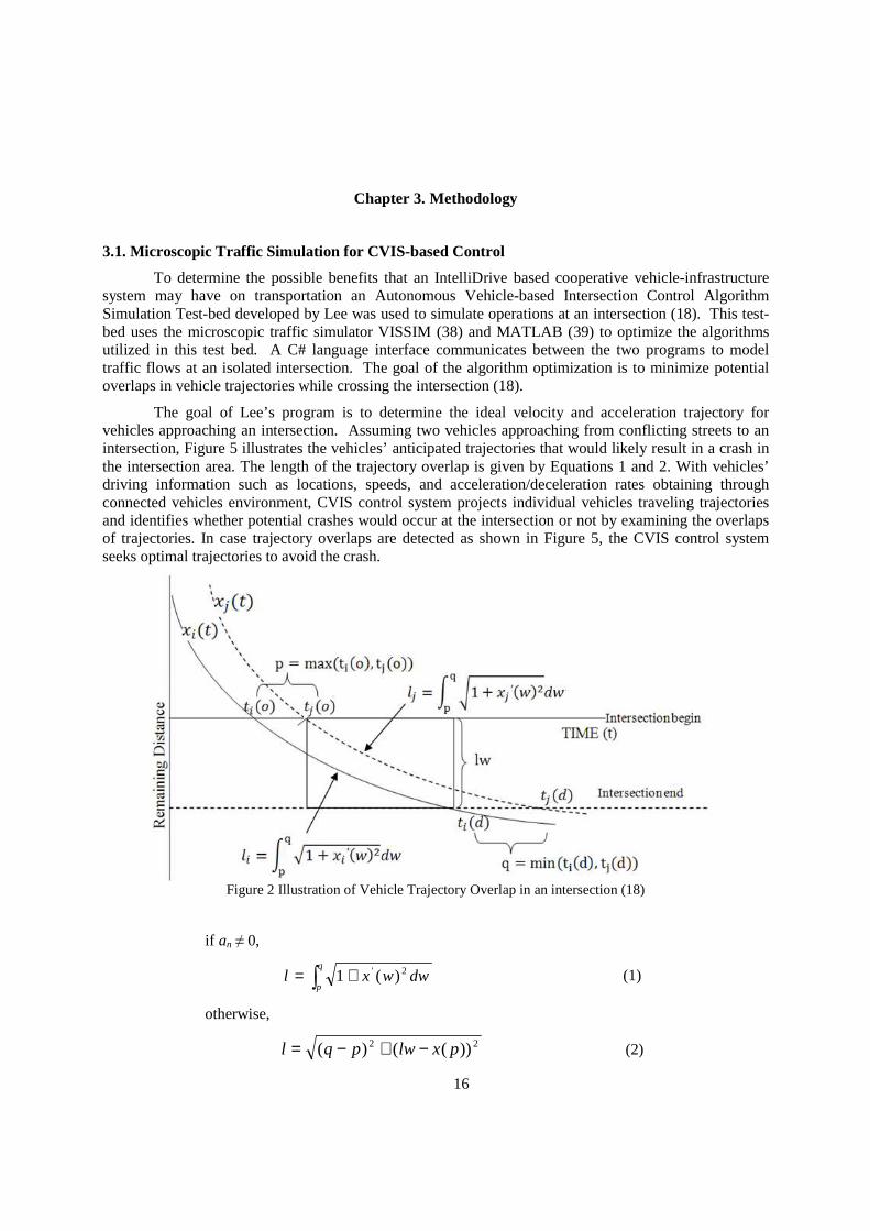
The goal of Lee’s program is to determine the ideal velocity and acceleration trajectory for vehicles approaching an intersection. Assuming two vehicles approaching from conflicting streets to an intersection, Figure 5 illustrates the vehicles’ anticipated trajectories that would likely result in a crash in the intersection area. The length of the trajectory overlap is given by Equations 1 and 2. With vehicles’ driving information such as locations, speeds, and acceleration/deceleration rates obtaining through connected vehicles environment, CVIS control system projects individual vehicles traveling trajectories and identifies whether potential crashes would occur at the intersection or not by examining the overlaps of trajectories. In case trajectory overlaps are detected as shown in Figure 5, the CVIS control system seeks optimal trajectories to avoid the crash.
Figure 2 Illustration of Vehicle Trajectory Overlap in an intersection (18)
if an ≠ 0,
∫ +=q
pdwwxl 2' )(1 (1)
otherwise,
22 ))(()( pxlwpql −+−= (2)
17
where:
)(txn: Predicted remaining distance to the intersection stop bar of vehicle n at time t
( tvtax nnn −−= 25.0)0( )
)0(nx : Current (t=0) remaining distance to the intersection stop bar of vehicle n at
p: Arrival time at the beginning of intersection
q: Arrival time at the end of intersection
lw: Intersection length in meters
an : Acceleration or Deceleration rate of vehicle n
vn : Current speed of vehicle n
t : time
To seek the optimal trajectories, the CVIS control system utilizes non-linear constraint optimization techniques, which are designed to solve an optimization problem given the Equations 3 through 6. With optimal acceleration/deceleration rate for each vehicle approaching to the intersection, the overlapping trajectory for each vehicle is adjusted to safely cross the intersection without stops or the need for a traffic signal. In case no feasible solutions are found, however, the CVIS control system runs in a recovery mode, a traffic signal-based special period designed to be quickly returned to normal optimization-based control mode (18).
∑∑∑∑∑∑∫= = = = = =
+=P
i
L
k
N
m
P
j
L
l
N
n
q
p ikm
i ik j jl
dwwxTLMin1 1 1 1 1 1
2' )(1 (3)
such that,
( ) mkitxx
vu
x
vaa
ikmikm
ikm
ikm
ikmikm ,,
)()0(2,
)0(2,max
22min
2
min ∀
−−−
≥ (4)
( ) mkitxx
vuaa
ikmikm
ikmikm ,,
)()0(2,min
22max
max ∀
−−≤ (5)
( ) 1,...2,1,0)((5.0 ,,,1,,,,2
,,1,, −=∀>++−−− ++ kimkimkimkimkimki NmandkiSRvvhaRaaS (6)
where,
P : Total phase numbers i, j : Phase number indices (1 if phases are conflicted, 0 otherwise) k, l: Lane identifier m, n: Vehicle identifier Li, Lj: Total number of lanes of phase i,j, respectively
Nik, Njl: Total number vehicles on lane k and l of phase i and j respectively. p: Arrival time at the beginning of intersection (= ( ))(),(max ,,,, otot nljmki )
q: Arrival time at the end of intersection (= ( ))(),(min ,,,, dtdt nljmki )
ti,k,m(o), tj,l,n(o) : Arrival times at the beginning of the intersection of vehicle m(n) on lane k(l) in phase i(j)
18
ti,k,m(d), tlj,l,n(d) : Arrival times at the end of the intersection of vehicle m(n) on lane k(l) in phase i(j)
)0()0(5.0 ,,1,,,,2
,, mkimkimkimki xxhvhaS ++−−=
( ))0(2 ,,1,,2
,,1,,11
,,1 mkimkimkimkimki xavvaR +++−+ ++−=
Before testing a series of volume cases, the original test bed is expanded upon to simulate a corridor of intersections rather than an isolated intersection. This decision was made because a corridor of intersections provides a slightly more realistic picture of regular operations than an isolated intersection. As discussed, Lee’s work provides source code and a detailed explanation of how the various components of the test bed operate (18). Each intersection is a one lane approach and departure on each of the four legs. The volume of vehicles varied in each case.
Ultimately, a 4 intersection corridor about 2800 meters long is used for simulation. Expanding the test-bed to accommodate more intersections required expansion of the VISSIM network and additional logic in the C# interface. The interface now has arrays of data store in most variables as opposed to single values. Intersections are optimized one at a time during each simulation second; the method for optimization has not changed. Lee’s work provides source code and a detailed explanation of how the various components of the test bed operate (18). Each intersection is a one lane approach and departure on each of the four legs. The volume of vehicles varied in each case.
Once the cooperative vehicle-infrastructure test bed was expanded upon and ready for simulation, 8 different volume cases were developed. The goal when selecting volume cases to be tested was to select a variety of volume cases that would reflect several volume-to-capacity (v/c) ratios and Level of Service (LOS) ratings. Both of these measures are based on traditional operations using non-cooperative infrastructure. In order to assess these measures, each potential volume case is modeled using Synchro (40). In Synchro, the optimized signal timing is determined and the resulting v/c ratio and LOS. Both v/c ratio and LOS are used because the v/c ratio is a common indicator for how well an intersection is operating, however, variations in signal timing will easily change the v/c ratio. LOS is based on signal delay therefore, average signal delay is substituted for LOS when developing volume cases. Table 1 that follows shows the 8 volume cases selected for simulation.
Table 1 Eight Volume Cases tested
Scenario Major Volume Cross Volume 1 900 500 2 900 600 3 800 500 4 800 400 5 600 500 6 600 400 7 400 400 8 400 300
Each volume case was run 5 times in the cooperative network and 5 times in the actuated signals network. Each repetition was 1860 simulation seconds long; the first 60 simulation seconds were used as a warm up period to populate the network (41). There were a total of 7 measures of effectiveness that were tested with each repetition, 4 for mobility and 3 for the environment. The mobility measures are tested to ensure that results are consistent with other studies and do not have an impact on the life cycle assessment. The mobility MOEs are total delay in hours, number of stops, average speed in kilometers per hour, and total travel time in hours. The environmental MOEs are carbon dioxide emissions in kilograms, fuel consumption in liters, and fuel economy in miles per gallon.
19
3.2 Safety Impact Assessment
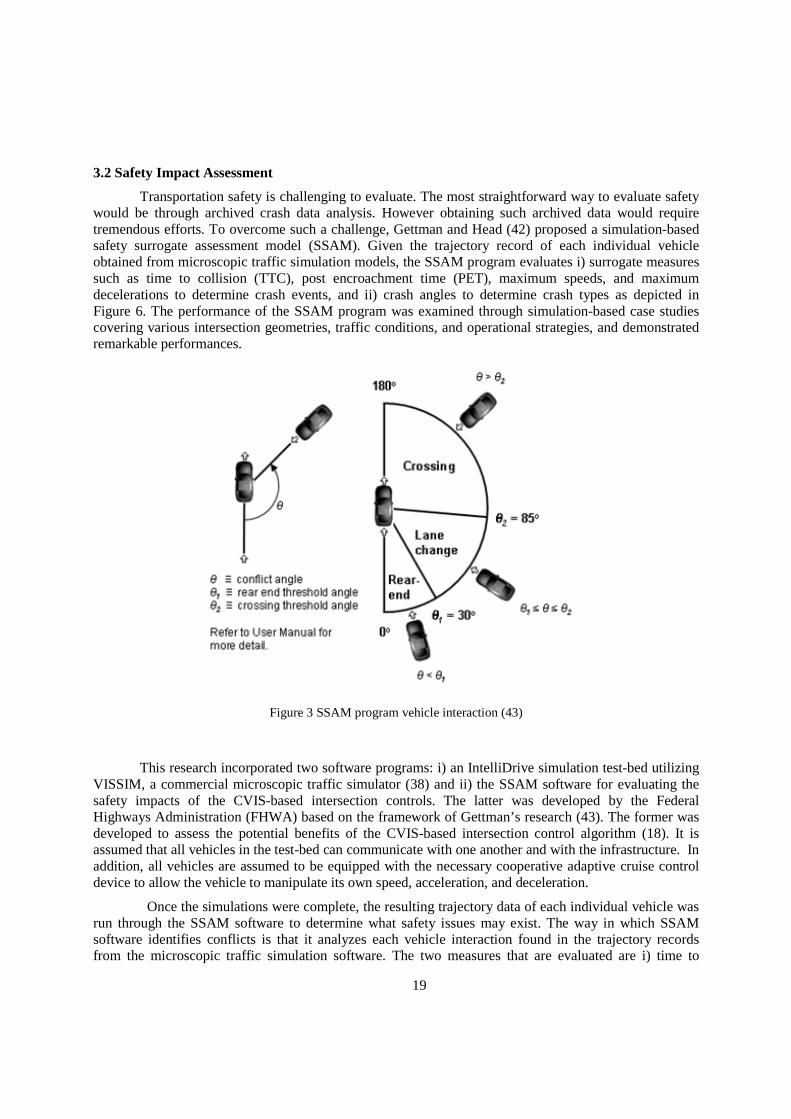
Transportation safety is challenging to evaluate. The most straightforward way to evaluate safety would be through archived crash data analysis. However obtaining such archived data would require tremendous efforts. To overcome such a challenge, Gettman and Head (42) proposed a simulation-based safety surrogate assessment model (SSAM). Given the trajectory record of each individual vehicle obtained from microscopic traffic simulation models, the SSAM program evaluates i) surrogate measures such as time to collision (TTC), post encroachment time (PET), maximum speeds, and maximum decelerations to determine crash events, and ii) crash angles to determine crash types as depicted in Figure 6. The performance of the SSAM program was examined through simulation-based case studies covering various intersection geometries, traffic conditions, and operational strategies, and demonstrated remarkable performances.
Figure 3 SSAM program vehicle interaction (43)
This research incorporated two software programs: i) an IntelliDrive simulation test-bed utilizing VISSIM, a commercial microscopic traffic simulator (38) and ii) the SSAM software for evaluating the safety impacts of the CVIS-based intersection controls. The latter was developed by the Federal Highways Administration (FHWA) based on the framework of Gettman’s research (43). The former was developed to assess the potential benefits of the CVIS-based intersection control algorithm (18). It is assumed that all vehicles in the test-bed can communicate with one another and with the infrastructure. In addition, all vehicles are assumed to be equipped with the necessary cooperative adaptive cruise control device to allow the vehicle to manipulate its own speed, acceleration, and deceleration.
Once the simulations were complete, the resulting trajectory data of each individual vehicle was run through the SSAM software to determine what safety issues may exist. The way in which SSAM software identifies conflicts is that it analyzes each vehicle interaction found in the trajectory records from the microscopic traffic simulation software. The two measures that are evaluated are i) time to
20
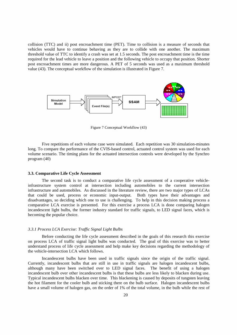
collision (TTC) and ii) post encroachment time (PET). Time to collision is a measure of seconds that vehicles would have to continue behaving as they are to collide with one another. The maximum threshold value of TTC to identify a crash was set at 1.5 seconds. The post encroachment time is the time required for the lead vehicle to leave a position and the following vehicle to occupy that position. Shorter post encroachment times are more dangerous. A PET of 5 seconds was used as a maximum threshold value (43). The conceptual workflow of the simulation is illustrated in Figure 7.
Figure 7 Conceptual Workflow (43)
Five repetitions of each volume case were simulated. Each repetition was 30 simulation-minutes long. To compare the performance of the CVIS-based control, actuated control system was used for each volume scenario. The timing plans for the actuated intersection controls were developed by the Synchro program (40)
3.3. Comparative Life Cycle Assessment
The second task is to conduct a comparative life cycle assessment of a cooperative vehicle-infrastructure system control at intersection including automobiles to the current intersection infrastructure and automobiles. As discussed in the literature review, there are two major types of LCAs that could be used, process or economic input-output. Both types have their advantages and disadvantages, so deciding which one to use is challenging. To help in this decision making process a comparative LCA exercise is presented. For this exercise a process LCA is done comparing halogen incandescent light bulbs, the former industry standard for traffic signals, to LED signal faces, which is becoming the popular choice.
3.3.1 Process LCA Exercise: Traffic Signal Light Bulbs
Before conducting the life cycle assessment described in the goals of this research this exercise on process LCA of traffic signal light bulbs was conducted. The goal of this exercise was to better understand process of life cycle assessment and help make key decisions regarding the methodology of the vehicle-intersection LCA which follows.
Incandescent bulbs have been used in traffic signals since the origin of the traffic signal. Currently, incandescent bulbs that are still in use in traffic signals are halogen incandescent bulbs, although many have been switched over to LED signal faces. The benefit of using a halogen incandescent bulb over other incandescent bulbs is that these bulbs are less likely to blacken during use. Typical incandescent bulbs blacken over time. This blackening is caused by deposits of tungsten leaving the hot filament for the cooler bulb and sticking there on the bulb surface. Halogen incandescent bulbs have a small volume of halogen gas, on the order of 1% of the total volume, in the bulb while the rest of
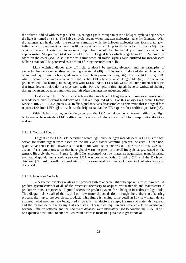
21
the volume is filled with inert gas. This 1% halogen gas is enough to cause a halogen cycle to begin when the light is turned on (44). The halogen cycle begins when tungsten molecules leave the filament. With the halogen gas in the bulb, the tungsten combines with the halogen molecules and forms a tungsten halide which by nature stays near the filament rather than sticking to the inner bulb surface (44). The obvious benefit of using an incandescent light bulb would be the initial purchase price which is approximately $12 per bulb (45) compared to the LED signal faces which range from $37 to $70 in price based on the color (45). Also, there was a time when all traffic signals were outfitted for incandescent bulbs so that could be perceived as a benefit of using incandescent bulbs.
Light emitting diodes give off light produced by moving electrons and the principles of electroluminescence rather than by heating a material (46). LEDs are a product of the semiconductor sector and require similar high grade materials and heavy manufacturing (46). The benefit to using LEDs where incandescent bulbs were once used is that LEDs have a much longer life (45). None of the problems with blackening bulbs happens with LEDs. Also, LEDs can withstand environmental hazards that incandescent bulbs do not cope well with. For example, traffic signals have to withstand shaking during inclement weather conditions and this often damages incandescent bulbs.
The drawback to LEDs is that to achieve the same level of brightness or luminous intensity as an incandescent bulb “several hundreds” of LEDs are required (47). For this analysis a General Electric Model: DR6-GCFB-20A green LED traffic signal face was disassembled to determine that the signal face requires 120 5mm LED lights to achieve the brightness that the ITE requires for a traffic signal face (48).
With this information, conducting a comparative LCA on halogen incandescent traffic signal light bulbs verses the equivalent LED traffic signal face seemed relevant and useful for transportation decision-makers.
3.3.1.1. Goal and Scope
The goal of the LCA is to determine which light bulb, halogen incandescent or LED, is the best option for traffic signal faces based on the life cycle global warming potential of each. Other non-quantitative benefits and drawbacks of each option will also be addressed. The scope of this LCA is to account for all emissions to air that have global warming potential overall lifecycle stages. Based on the generic lifecycle shown in Figure 3, this LCA accounted for raw materials acquisition, manufacturing, use, and disposal. As stated, a process LCA was conducted using SimaPro (24) and the Ecoinvent database (27). Additionally, an analysis of costs associated with each of these technologies was also discussed.
3.3.1.2. Inventory Analysis:
To begin the inventory analysis the product system of each light bulb type must be determined. A product system consists of all of the processes necessary to acquire raw materials and manufacture a product with its components. Figure 8 shows the product system for a halogen incandescent light bulb. This diagram shows all of the steps from raw materials acquisition, through the entire manufacturing process, right up to the completed product. This figure is lacking some detail in how raw materials are acquired, what machines are being used at various manufacturing steps, the mass of materials required, and the magnitude of energy input at each step. These data requirements were able to be overlooked because SimaPro software and the Ecoinvent database were ultimately used to conduct the LCA. It will be explained how SimaPro and the Ecoinvent database made this possible in greater detail.
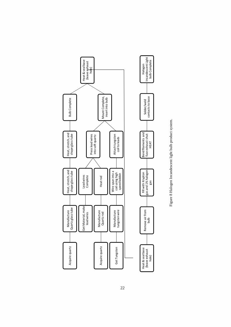
22
Ha
log
en
In
can
de
sce
nt
Lig
ht
bu
lb C
om
ple
te
Sold
er/
we
ld
con
tact
s to
ba
se
Be
nd
fila
me
nts
an
d
fuse
exh
au
st s
hu
t:
HE
AT
Fill
wit
h K
ryp
ton
g
as
an
d 1
% h
alo
ge
n
ga
s
Re
mo
ve a
ir f
rom
b
ulb
He
at
& s
ea
l ba
se
(le
ave
exh
au
st
ho
le)
He
at
& s
ea
l ba
se
(le
ave
exh
au
st
ho
le)
Bu
lb C
om
ple
teH
ea
t, s
tre
tch
, an
d
sha
pe
gla
ss t
ub
eH
ea
t, s
tre
tch
, an
d
sha
pe
gla
ss t
ub
eM
an
ufa
ctu
re
Qu
art
z g
lass
tu
be
Acq
uir
e q
ua
rtz
Mo
un
t C
om
ple
te,
inse
rt in
to b
ulb
Pre
ss le
ad
wir
es
into
so
ft q
ua
rtz
Lea
d w
ire
s C
om
ple
teG
et
Ma
teri
al,
ma
ke
lea
d w
ire
s
He
at
rod
Ma
nu
fact
ure
Q
ua
rtz
rod
Acq
uir
e q
ua
rtz
Att
ach
tu
ng
ste
n
coil
to le
ad
s
Wir
e s
pu
n in
to a
co
il u
sin
g h
igh
sp
ee
d b
ob
bin
Ma
nu
fact
ure
tu
ng
ste
n w
ire
Ge
t T
un
gst
en
Fig
ure
8 H
alo
gen
Inca
nde
sce
nt
light
bul
b pr
oduc
t sy
stem
.
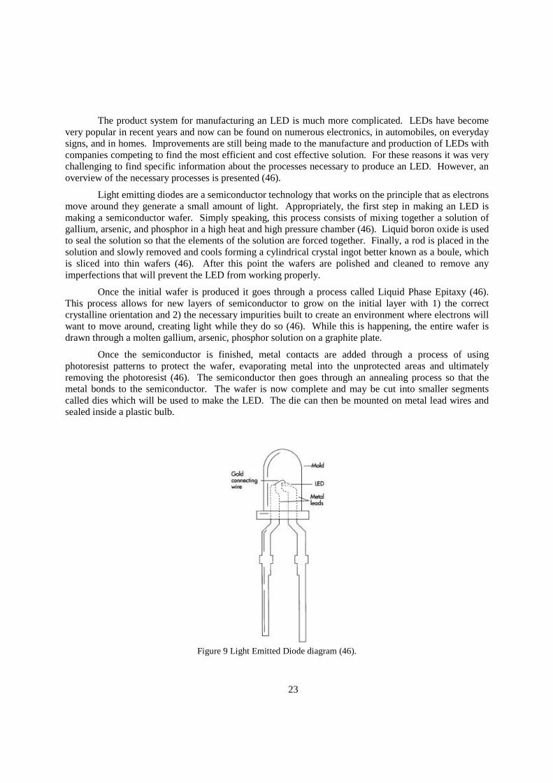
23
The product system for manufacturing an LED is much more complicated. LEDs have become very popular in recent years and now can be found on numerous electronics, in automobiles, on everyday signs, and in homes. Improvements are still being made to the manufacture and production of LEDs with companies competing to find the most efficient and cost effective solution. For these reasons it was very challenging to find specific information about the processes necessary to produce an LED. However, an overview of the necessary processes is presented (46).
Light emitting diodes are a semiconductor technology that works on the principle that as electrons move around they generate a small amount of light. Appropriately, the first step in making an LED is making a semiconductor wafer. Simply speaking, this process consists of mixing together a solution of gallium, arsenic, and phosphor in a high heat and high pressure chamber (46). Liquid boron oxide is used to seal the solution so that the elements of the solution are forced together. Finally, a rod is placed in the solution and slowly removed and cools forming a cylindrical crystal ingot better known as a boule, which is sliced into thin wafers (46). After this point the wafers are polished and cleaned to remove any imperfections that will prevent the LED from working properly.
Once the initial wafer is produced it goes through a process called Liquid Phase Epitaxy (46). This process allows for new layers of semiconductor to grow on the initial layer with 1) the correct crystalline orientation and 2) the necessary impurities built to create an environment where electrons will want to move around, creating light while they do so (46). While this is happening, the entire wafer is drawn through a molten gallium, arsenic, phosphor solution on a graphite plate.
Once the semiconductor is finished, metal contacts are added through a process of using photoresist patterns to protect the wafer, evaporating metal into the unprotected areas and ultimately removing the photoresist (46). The semiconductor then goes through an annealing process so that the metal bonds to the semiconductor. The wafer is now complete and may be cut into smaller segments called dies which will be used to make the LED. The die can then be mounted on metal lead wires and sealed inside a plastic bulb.
Figure 9 Light Emitted Diode diagram (46).
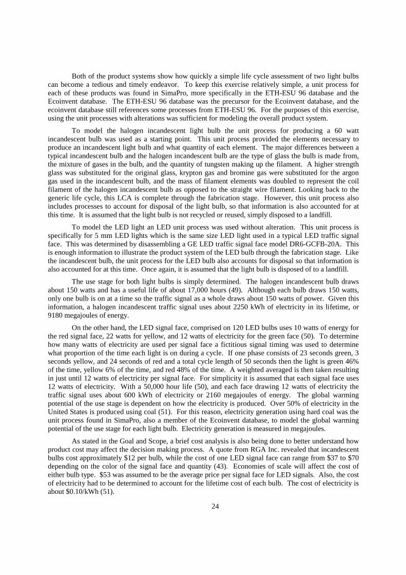
24
Both of the product systems show how quickly a simple life cycle assessment of two light bulbs can become a tedious and timely endeavor. To keep this exercise relatively simple, a unit process for each of these products was found in SimaPro, more specifically in the ETH-ESU 96 database and the Ecoinvent database. The ETH-ESU 96 database was the precursor for the Ecoinvent database, and the ecoinvent database still references some processes from ETH-ESU 96. For the purposes of this exercise, using the unit processes with alterations was sufficient for modeling the overall product system.
To model the halogen incandescent light bulb the unit process for producing a 60 watt incandescent bulb was used as a starting point. This unit process provided the elements necessary to produce an incandescent light bulb and what quantity of each element. The major differences between a typical incandescent bulb and the halogen incandescent bulb are the type of glass the bulb is made from, the mixture of gases in the bulb, and the quantity of tungsten making up the filament. A higher strength glass was substituted for the original glass, krypton gas and bromine gas were substituted for the argon gas used in the incandescent bulb, and the mass of filament elements was doubled to represent the coil filament of the halogen incandescent bulb as opposed to the straight wire filament. Looking back to the generic life cycle, this LCA is complete through the fabrication stage. However, this unit process also includes processes to account for disposal of the light bulb, so that information is also accounted for at this time. It is assumed that the light bulb is not recycled or reused, simply disposed to a landfill.
To model the LED light an LED unit process was used without alteration. This unit process is specifically for 5 mm LED lights which is the same size LED light used in a typical LED traffic signal face. This was determined by disassembling a GE LED traffic signal face model DR6-GCFB-20A. This is enough information to illustrate the product system of the LED bulb through the fabrication stage. Like the incandescent bulb, the unit process for the LED bulb also accounts for disposal so that information is also accounted for at this time. Once again, it is assumed that the light bulb is disposed of to a landfill.
The use stage for both light bulbs is simply determined. The halogen incandescent bulb draws about 150 watts and has a useful life of about 17,000 hours (49). Although each bulb draws 150 watts, only one bulb is on at a time so the traffic signal as a whole draws about 150 watts of power. Given this information, a halogen incandescent traffic signal uses about 2250 kWh of electricity in its lifetime, or 9180 megajoules of energy.
On the other hand, the LED signal face, comprised on 120 LED bulbs uses 10 watts of energy for the red signal face, 22 watts for yellow, and 12 watts of electricity for the green face (50). To determine how many watts of electricity are used per signal face a fictitious signal timing was used to determine what proportion of the time each light is on during a cycle. If one phase consists of 23 seconds green, 3 seconds yellow, and 24 seconds of red and a total cycle length of 50 seconds then the light is green 46% of the time, yellow 6% of the time, and red 48% of the time. A weighted averaged is then taken resulting in just until 12 watts of electricity per signal face. For simplicity it is assumed that each signal face uses 12 watts of electricity. With a 50,000 hour life (50), and each face drawing 12 watts of electricity the traffic signal uses about 600 kWh of electricity or 2160 megajoules of energy. The global warming potential of the use stage is dependent on how the electricity is produced. Over 50% of electricity in the United States is produced using coal (51). For this reason, electricity generation using hard coal was the unit process found in SimaPro, also a member of the Ecoinvent database, to model the global warming potential of the use stage for each light bulb. Electricity generation is measured in megajoules.
As stated in the Goal and Scope, a brief cost analysis is also being done to better understand how product cost may affect the decision making process. A quote from RGA Inc. revealed that incandescent bulbs cost approximately $12 per bulb, while the cost of one LED signal face can range from $37 to $70 depending on the color of the signal face and quantity (43). Economies of scale will affect the cost of either bulb type. $53 was assumed to be the average price per signal face for LED signals. Also, the cost of electricity had to be determined to account for the lifetime cost of each bulb. The cost of electricity is about $0.10/kWh (51).
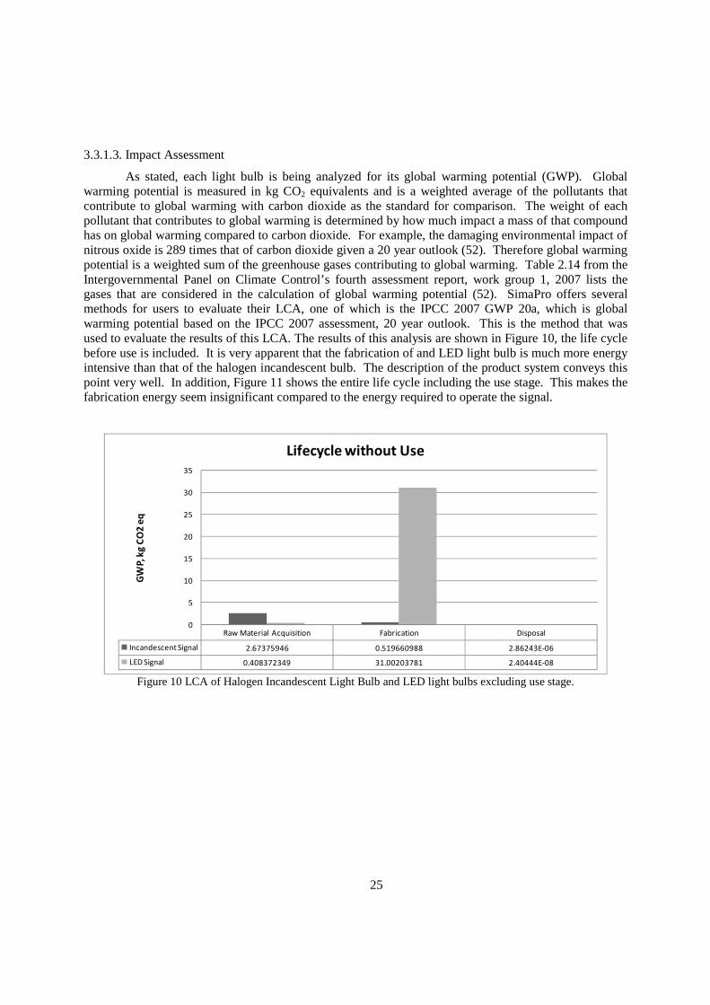
25
3.3.1.3. Impact Assessment
As stated, each light bulb is being analyzed for its global warming potential (GWP). Global warming potential is measured in kg CO2 equivalents and is a weighted average of the pollutants that contribute to global warming with carbon dioxide as the standard for comparison. The weight of each pollutant that contributes to global warming is determined by how much impact a mass of that compound has on global warming compared to carbon dioxide. For example, the damaging environmental impact of nitrous oxide is 289 times that of carbon dioxide given a 20 year outlook (52). Therefore global warming potential is a weighted sum of the greenhouse gases contributing to global warming. Table 2.14 from the Intergovernmental Panel on Climate Control’s fourth assessment report, work group 1, 2007 lists the gases that are considered in the calculation of global warming potential (52). SimaPro offers several methods for users to evaluate their LCA, one of which is the IPCC 2007 GWP 20a, which is global warming potential based on the IPCC 2007 assessment, 20 year outlook. This is the method that was used to evaluate the results of this LCA. The results of this analysis are shown in Figure 10, the life cycle before use is included. It is very apparent that the fabrication of and LED light bulb is much more energy intensive than that of the halogen incandescent bulb. The description of the product system conveys this point very well. In addition, Figure 11 shows the entire life cycle including the use stage. This makes the fabrication energy seem insignificant compared to the energy required to operate the signal.
Raw Material Acquisition Fabrication Disposal
Incandescent Signal 2.67375946 0.519660988 2.86243E-06
LED Signal 0.408372349 31.00203781 2.40444E-08
0
5
10
15
20
25
30
35
GW
P, k
g C
O2
eq
Lifecycle without Use
Figure 10 LCA of Halogen Incandescent Light Bulb and LED light bulbs excluding use stage.
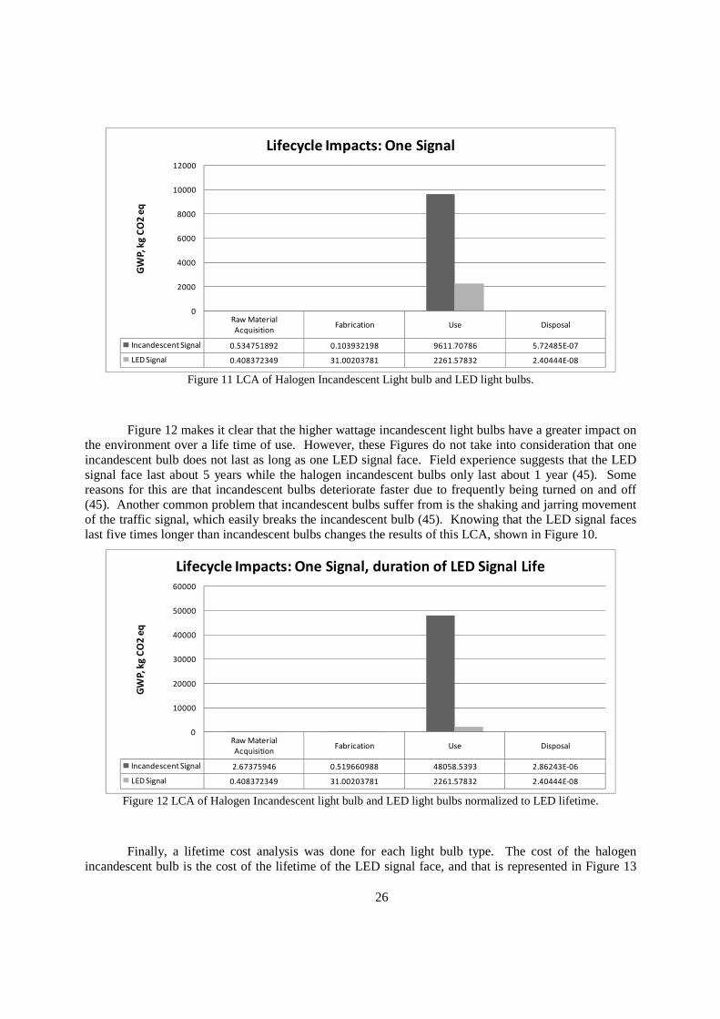
26
Raw Material
AcquisitionFabrication Use Disposal
Incandescent Signal 0.534751892 0.103932198 9611.70786 5.72485E-07
LED Signal 0.408372349 31.00203781 2261.57832 2.40444E-08
0
2000
4000
6000
8000
10000
12000
GW
P, k
g C
O2
eq
Lifecycle Impacts: One Signal
Figure 11 LCA of Halogen Incandescent Light bulb and LED light bulbs.
Figure 12 makes it clear that the higher wattage incandescent light bulbs have a greater impact on the environment over a life time of use. However, these Figures do not take into consideration that one incandescent bulb does not last as long as one LED signal face. Field experience suggests that the LED signal face last about 5 years while the halogen incandescent bulbs only last about 1 year (45). Some reasons for this are that incandescent bulbs deteriorate faster due to frequently being turned on and off (45). Another common problem that incandescent bulbs suffer from is the shaking and jarring movement of the traffic signal, which easily breaks the incandescent bulb (45). Knowing that the LED signal faces last five times longer than incandescent bulbs changes the results of this LCA, shown in Figure 10.
Raw Material
AcquisitionFabrication Use Disposal
Incandescent Signal 2.67375946 0.519660988 48058.5393 2.86243E-06
LED Signal 0.408372349 31.00203781 2261.57832 2.40444E-08
0
10000
20000
30000
40000
50000
60000
GW
P, k
g C
O2
eq
Lifecycle Impacts: One Signal, duration of LED Signal Life
Figure 12 LCA of Halogen Incandescent light bulb and LED light bulbs normalized to LED lifetime.
Finally, a lifetime cost analysis was done for each light bulb type. The cost of the halogen incandescent bulb is the cost of the lifetime of the LED signal face, and that is represented in Figure 13
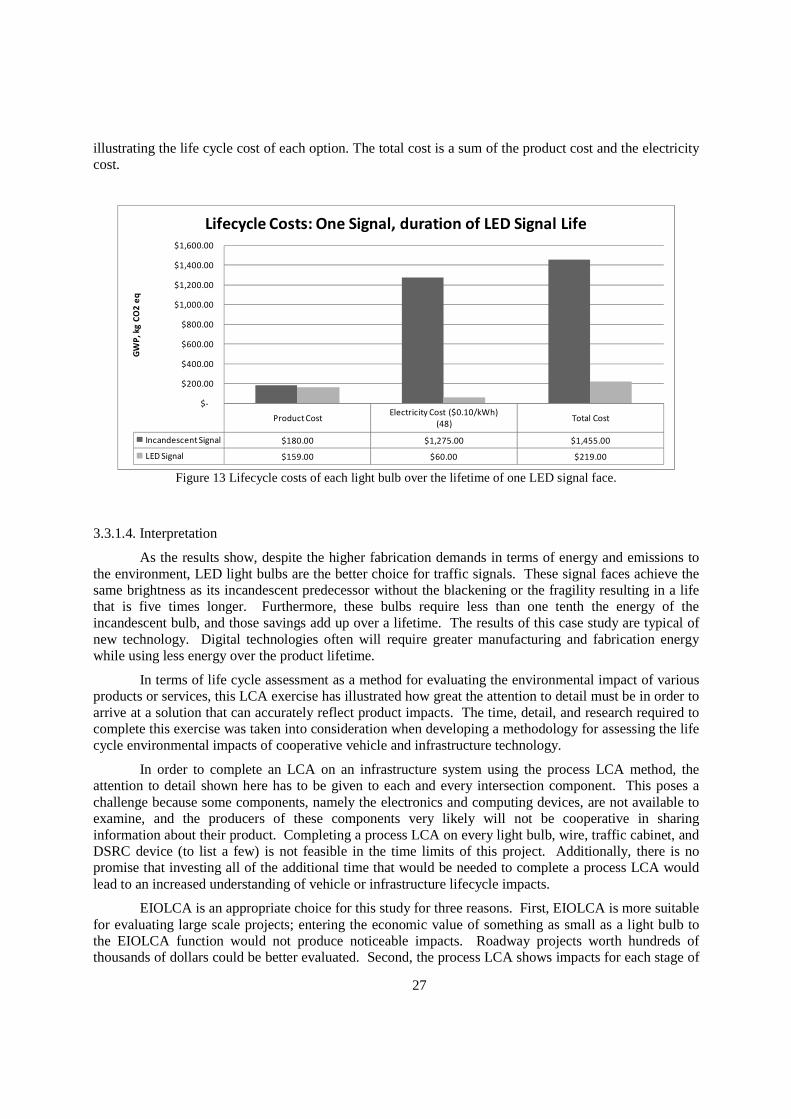
27
illustrating the life cycle cost of each option. The total cost is a sum of the product cost and the electricity cost.
Product CostElectricity Cost ($0.10/kWh)
(48)Total Cost
Incandescent Signal $180.00 $1,275.00 $1,455.00
LED Signal $159.00 $60.00 $219.00
$-
$200.00
$400.00
$600.00
$800.00
$1,000.00
$1,200.00
$1,400.00
$1,600.00
GW
P,
kg
CO
2 e
q
Lifecycle Costs: One Signal, duration of LED Signal Life
Figure 13 Lifecycle costs of each light bulb over the lifetime of one LED signal face.
3.3.1.4. Interpretation
As the results show, despite the higher fabrication demands in terms of energy and emissions to the environment, LED light bulbs are the better choice for traffic signals. These signal faces achieve the same brightness as its incandescent predecessor without the blackening or the fragility resulting in a life that is five times longer. Furthermore, these bulbs require less than one tenth the energy of the incandescent bulb, and those savings add up over a lifetime. The results of this case study are typical of new technology. Digital technologies often will require greater manufacturing and fabrication energy while using less energy over the product lifetime.
In terms of life cycle assessment as a method for evaluating the environmental impact of various products or services, this LCA exercise has illustrated how great the attention to detail must be in order to arrive at a solution that can accurately reflect product impacts. The time, detail, and research required to complete this exercise was taken into consideration when developing a methodology for assessing the life cycle environmental impacts of cooperative vehicle and infrastructure technology.
In order to complete an LCA on an infrastructure system using the process LCA method, the attention to detail shown here has to be given to each and every intersection component. This poses a challenge because some components, namely the electronics and computing devices, are not available to examine, and the producers of these components very likely will not be cooperative in sharing information about their product. Completing a process LCA on every light bulb, wire, traffic cabinet, and DSRC device (to list a few) is not feasible in the time limits of this project. Additionally, there is no promise that investing all of the additional time that would be needed to complete a process LCA would lead to an increased understanding of vehicle or infrastructure lifecycle impacts.
EIOLCA is an appropriate choice for this study for three reasons. First, EIOLCA is more suitable for evaluating large scale projects; entering the economic value of something as small as a light bulb to the EIOLCA function would not produce noticeable impacts. Roadway projects worth hundreds of thousands of dollars could be better evaluated. Second, the process LCA shows impacts for each stage of
28
the product life. If one were studying the changes during a single stage of a product’s production the granularity of the process LCA would be necessary. This project, however, is substituting whole components for one another, this can be analyzed through EIOLCA. Third, the accuracy of any LCA is based on the accuracy of data input. Studies have been done on the cost and benefits of implementing IntelliDrive systems in the US. Accurate pricing data from reliable sources is available to input to the EIOLCA. Therefore, economic input-output life cycle assessment is the chosen method of LCA for this study.
The sections that follow detail the methods used to complete the EIOLCA on the cooperative vehicle-infrastructure system and the current transportation system.
3.3.2. Goal and Scope
The goal of this LCA is to determine how the traditional transportation infrastructure system compares to a cooperative vehicle-infrastructure system in terms of CO2 emissions and energy use. The traditional infrastructure system is made up of vehicles whose movements are governed by a traffic signal, likely an actuated one. The cooperative vehicle-infrastructure system is made up of cooperative vehicles whose movements are governed by a roadside unit. Carbon dioxide and energy use will be referred to as the impacts. Both of these scenarios assume that there is no intersection control already present, which is unlikely. A third scenario considered is the conversion of the current transportation infrastructure to a cooperative system. Realistically speaking, this is probably the most likely scenario to occur if cooperative infrastructure were implemented. These comparisons are valuable because IntelliDrive technology has potential to reduce fuel consumption during vehicle use; however, requires greater communications electronics and computing power in order to make mobility improvements possible.
The scope accounts for the lifecycle from materials extraction through the use portion of the lifecycle. The remaining stages, disposal, reuse, recycling, and landfill, will not be addressed in this LCA because those stages are identical for both scenarios. The vehicle, current or cooperative, would be scrapped for recycle and reuse. The OBU would be treated in the same way as any of the other electronic components that make up vehicles today. In terms of infrastructure, controller equipment is repaired and refurbished many times over its very long life and RSU equipment would see the same treatment. Also, if the assumption were made that all components are landfilled once they can no longer be refurbished then that would not impact greenhouse gases emissions or energy use. Because the end-of-life processes in each scenario are the same, they will not be analyzed. For the current and cooperative vehicles, a single vehicle will be the functional unit. For the intersections a complete intersection is the functional unit. Ultimately, the impacts of the intersection LCA will be divided over the number of vehicles that are estimated to use each intersection.
3.3.3. Inventory Analysis:
The primary task in inventory analysis is data collection. Three reports were the key to the data collection process (14, 53, 54). Each of these three resources provides very detailed information about the components, installation and pricing for the OBU and RSU. The Virginia Department of Transportation (VDOT) Bid database was used for current infrastructure pricing estimates (55).
This analysis consists of three possible scenarios.
1. Current Scenario: a current vehicle operating at a signalized intersection.
2. Cooperative scenario: cooperative vehicle-infrastructure system, an OBU equipped vehicle operating at a cooperative intersection with RSU.
29
3. Conversion scenario: Result of converting traditional infrastructure to cooperative. This scenario assumes cooperative vehicles.
The assumption to test scenarios with 100% cooperatively equipped vehicles was necessary for the CVIS test-bed to work properly. Additionally, this assumption is not an unreasonable one given that the USDOT is moving towards mandating that new vehicles being manufactured come equipped with IntelliDrive communications equipment so that there will be vehicles ready to use IntelliDrive infrastructure once installed. This mandate could start as soon as 2013 (56).
The difference between the current vehicle and the cooperative vehicle is quite simple, the cooperative vehicle is outfit with an OBU. The individual components of the OBU are explained in this section. The differences between the current intersection and the cooperative intersection may be less apparent. A signalized intersection consists of the obvious traffic signals, mast arms, poles, and a controller box, as well as, lengths of pipe and wires below ground that allow the system to operate. The cooperative, IntelliDrive equipped scenario, would not require the same components. Because the vehicle and the infrastructure are communicating, traffic signal heads are obsolete. The cooperative system would require only an RSU, which is comprised of several electronic components housed in a cabinet, and a pole to mount an antenna on in order to send and receive information.
To simplify the analysis, the various elements divided into subsystems: automobile, OBU, signalized intersection, cooperative intersection, and conversion intersection. The conversion intersection reflects the costs of removing unnecessary infrastructure and installing the components necessary for cooperative operations. Pricing was determined by subsystem as described below. Tables showing the complete list of items evaluated can be found in the appendix.
3.3.3.1. Automobile
First, the price of the vehicle is the Kelley Blue Book base invoice price of an average 2009 passenger vehicle, represented by the Ford Taurus (57). This price eliminates unnecessary taxes and price hikes that do not reflect emissions, simply profits.
The only difference between the current available automobile and a cooperative automobile is the fuel efficiency, mpg, of each and the addition of the OBU to the cooperative vehicle. The general framework for an automobile EIOLCA was found in (23), and built upon with the cooperative technology components.
3.3.3.2. OBU
The OBU has been priced at $50 for an LCD display, a radio antenna, a positioning device, and a data processing unit. This estimate is from the USDOT cost benefit analysis (53) and represents the cost at the assembly line.
3.3.3.3. Signalized Intersection
Pricing for all of the components of the current intersection was found in the Virginia Department of Transportation Bid database (55). This database is an itemized record of what contractors have bid for jobs statewide for the last three years.
The total cost of each intersection scenario should not be taken as an appropriate estimate for the cost of constructing a signalized intersection. When doing a comparative LCA it is entirely appropriate to

30
ignore redundant costs, costs that are necessary for both scenarios. Many redundant costs have been ignored as well as costs related to design work and preliminary engineering. The components that make up the current intersection and the cooperative intersection for this study are alternatives for one another. A final note about ignoring redundant costs, for the automobile section of this analysis it would have been completely appropriate to ignore the cost of the automobile, maintenance, and insurance, however, those costs were included as part of this study to better illustrate EIOLCA.
3.3.3.4. RSU:
The RSU pricing estimates came primarily from the Intellimotion article mentioned earlier (54). This article provides average pricing for the necessary components to install a working RSU. The ones described were constructed for a test corridor in California. Only one key cooperative component is not specifically listed in this article is the multiband configurable networking unit, MCNU. This component is the ‘brains’ of the RSU operations. Because pricing data for this component was not available from any retailer, it was estimated at $5,000 a price that one may expect to pay for a highly sophisticated computer with a great deal of computing capacity.
3.3.3.5. Conversion:
The conversion scenario assumes cooperative vehicles. Conversion describes the components needed to change a signalized intersection into a cooperative, IntelliDrive equipped intersection. The majority of the construction costs are no longer needed because wiring, electricity, and foundations are already present. This scenario is most likely what will occur as IntelliDrive technologies are deployed. The pricing for this scenario draws from the signalized and cooperative scenarios.
3.3.4. Impact Assessment
Once costs for all components of all subsystems were found, they are converted to 1997 dollars so they can be input into the Carnegie Mellon’s Green Design Institute EIOLCA tool (29). Both the web based tool and the MATLAB function tool were used to complete this process. The tool requires 1997 dollar costs to an economic sector and outputs carbon emissions data and total energy data. The output is tabulated to see where potential weaknesses exist and how improvements could be made.
3.4 Automobile Use as Stage of LCA
The first step to integrating the results from task 1 into the LCA was to develop an aggregate fuel economy. Task 1 tested 8 different volume cases but only one fuel economy can be taken into consideration. The aggregate fuel economy is used to determine how much fuel must be purchased over the lifetime of the vehicle. Fuel production must be taken into consideration as part of the life cycle assessment because that process also contributes to greenhouse gas emissions and global warming. The aggregate fuel economy was determined by doing a weighted average of all 8 volume cases. Weights represented the portion of time each day that a particular volume case might be taking place at an intersection.
In order to estimate the price of gasoline, statistics about the wholesale price of gas were found in the Energy Information Administration (EIA) Short term energy outlook report. The price per gallon of fuel was found to be $1.761 in 2009 (58). This value excludes taxes and small price hikes by gasoline providers for profit, leaving only the producer price. Taxes and price hikes inflate the outputs of this analysis. The price of gasoline is so variable from one year to the next that the 2009 price is assumed to
31
be constant over the entire lifetime of the vehicle. Regardless of the price of fuel in a year, it should convert to approximately the same value in 1997 dollars for using the EIOLCA tool. Lifetime vehicle miles traveled was determined using AAA information (59). Given the fuel economy calculated and that the average life of an automobile is about 16.1 year, the total lifetime costs of a vehicle can be calculated (60).
To maintain consistency throughout the LCA, the CO2 emissions and fuel consumption of both the control and cooperative vehicles was calculated based on the number of gallons of gas that the vehicle is assumed to use over its lifetime. One gallon of regular, unleaded gasoline emits 8,788 grams of CO2 into the atmosphere (61). Similarly, the energy use by the vehicle can be calculated using the lifetime gasoline use multiplied by 120381.890 kilojoules of energy per gallon of gasoline (62). By using this method it is clear that the amount of gasoline being paid for is the same as is being used over the life of the vehicle.
Finally, the last two costs that need to be accounted for over the vehicle use period are maintenance and repair costs and insurance costs. Association, AAA, has released a 2009 edition of “Your Driving Costs” outlining other costs of driving (59). This resource was used to estimate the average cost of annual maintenance and insurance for a driver.
One additional assumption is that the owner would have to replace the OBU once in the life of the vehicle; this is not unreasonable because many of the mechanical parts of the vehicle are fully replaced one or more times. Also, maintenance costs are estimated at approximately $1 per year (53).
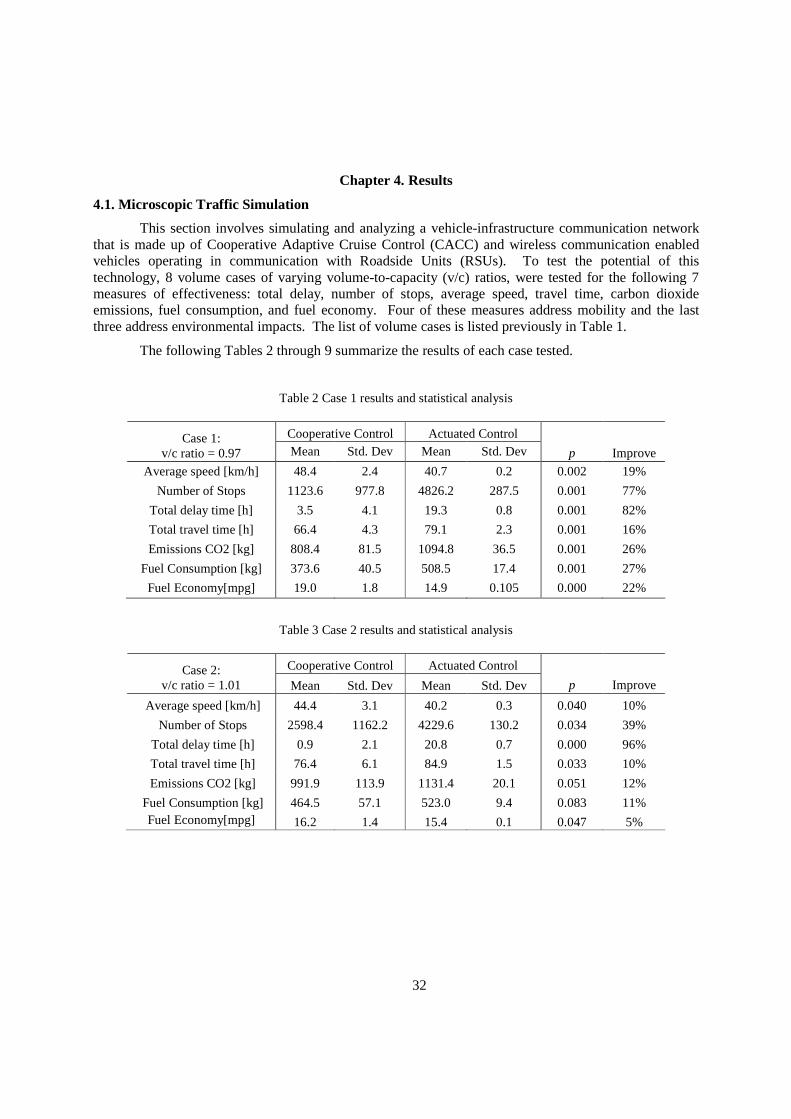
32
Chapter 4. Results
4.1. Microscopic Traffic Simulation
This section involves simulating and analyzing a vehicle-infrastructure communication network that is made up of Cooperative Adaptive Cruise Control (CACC) and wireless communication enabled vehicles operating in communication with Roadside Units (RSUs). To test the potential of this technology, 8 volume cases of varying volume-to-capacity (v/c) ratios, were tested for the following 7 measures of effectiveness: total delay, number of stops, average speed, travel time, carbon dioxide emissions, fuel consumption, and fuel economy. Four of these measures address mobility and the last three address environmental impacts. The list of volume cases is listed previously in Table 1.
The following Tables 2 through 9 summarize the results of each case tested.
Table 2 Case 1 results and statistical analysis
Cooperative Control Actuated Control Case 1: v/c ratio = 0.97 Mean Std. Dev Mean Std. Dev p Improve
Average speed [km/h] 48.4 2.4 40.7 0.2 0.002 19%
Number of Stops 1123.6 977.8 4826.2 287.5 0.001 77%
Total delay time [h] 3.5 4.1 19.3 0.8 0.001 82%
Total travel time [h] 66.4 4.3 79.1 2.3 0.001 16%
Emissions CO2 [kg] 808.4 81.5 1094.8 36.5 0.001 26%
Fuel Consumption [kg] 373.6 40.5 508.5 17.4 0.001 27%
Fuel Economy[mpg] 19.0 1.8 14.9 0.105 0.000 22%
Table 3 Case 2 results and statistical analysis
Cooperative Control Actuated Control Case 2: v/c ratio = 1.01 Mean Std. Dev Mean Std. Dev p Improve
Average speed [km/h] 44.4 3.1 40.2 0.3 0.040 10%
Number of Stops 2598.4 1162.2 4229.6 130.2 0.034 39%
Total delay time [h] 0.9 2.1 20.8 0.7 0.000 96%
Total travel time [h] 76.4 6.1 84.9 1.5 0.033 10%
Emissions CO2 [kg] 991.9 113.9 1131.4 20.1 0.051 12%
Fuel Consumption [kg] 464.5 57.1 523.0 9.4 0.083 11% Fuel Economy[mpg] 16.2 1.4 15.4 0.1 0.047 5%
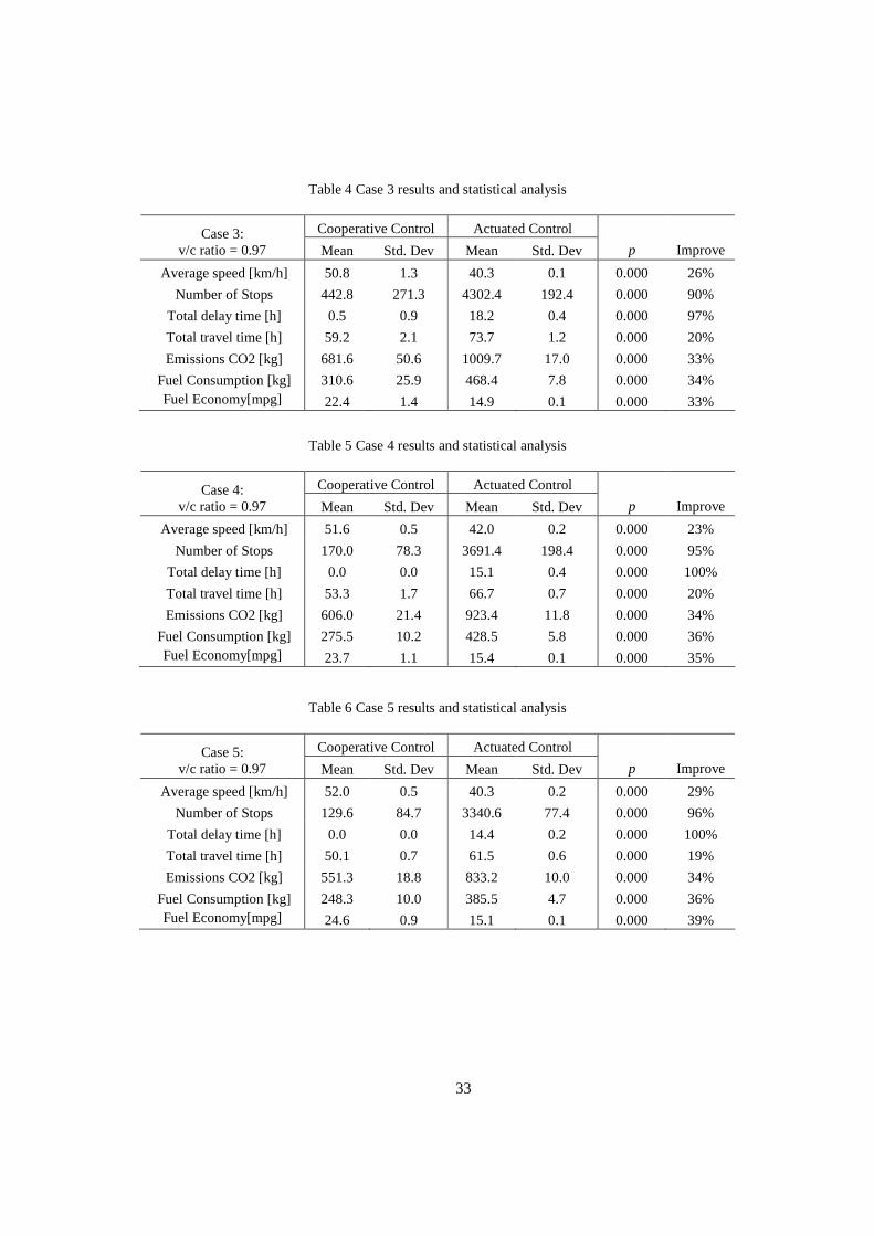
33
Table 4 Case 3 results and statistical analysis
Cooperative Control Actuated Control Case 3: v/c ratio = 0.97 Mean Std. Dev Mean Std. Dev p Improve
Average speed [km/h] 50.8 1.3 40.3 0.1 0.000 26%
Number of Stops 442.8 271.3 4302.4 192.4 0.000 90%
Total delay time [h] 0.5 0.9 18.2 0.4 0.000 97%
Total travel time [h] 59.2 2.1 73.7 1.2 0.000 20%
Emissions CO2 [kg] 681.6 50.6 1009.7 17.0 0.000 33%
Fuel Consumption [kg] 310.6 25.9 468.4 7.8 0.000 34% Fuel Economy[mpg] 22.4 1.4 14.9 0.1 0.000 33%
Table 5 Case 4 results and statistical analysis
Cooperative Control Actuated Control Case 4: v/c ratio = 0.97 Mean Std. Dev Mean Std. Dev p Improve
Average speed [km/h] 51.6 0.5 42.0 0.2 0.000 23%
Number of Stops 170.0 78.3 3691.4 198.4 0.000 95%
Total delay time [h] 0.0 0.0 15.1 0.4 0.000 100%
Total travel time [h] 53.3 1.7 66.7 0.7 0.000 20%
Emissions CO2 [kg] 606.0 21.4 923.4 11.8 0.000 34%
Fuel Consumption [kg] 275.5 10.2 428.5 5.8 0.000 36% Fuel Economy[mpg] 23.7 1.1 15.4 0.1 0.000 35%
Table 6 Case 5 results and statistical analysis
Cooperative Control Actuated Control Case 5: v/c ratio = 0.97 Mean Std. Dev Mean Std. Dev p Improve
Average speed [km/h] 52.0 0.5 40.3 0.2 0.000 29%
Number of Stops 129.6 84.7 3340.6 77.4 0.000 96%
Total delay time [h] 0.0 0.0 14.4 0.2 0.000 100%
Total travel time [h] 50.1 0.7 61.5 0.6 0.000 19%
Emissions CO2 [kg] 551.3 18.8 833.2 10.0 0.000 34%
Fuel Consumption [kg] 248.3 10.0 385.5 4.7 0.000 36% Fuel Economy[mpg] 24.6 0.9 15.1 0.1 0.000 39%
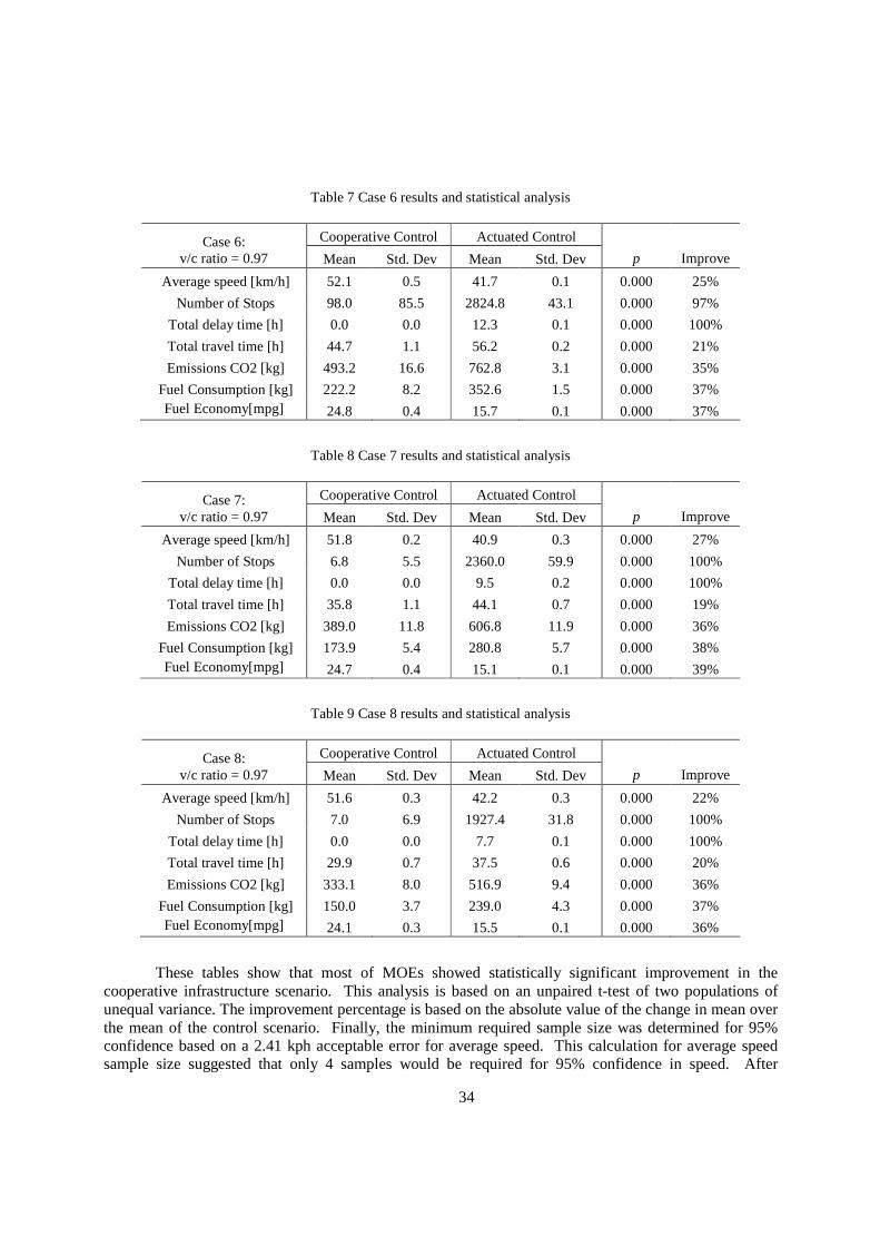
34
Table 7 Case 6 results and statistical analysis
Cooperative Control Actuated Control Case 6: v/c ratio = 0.97 Mean Std. Dev Mean Std. Dev p Improve
Average speed [km/h] 52.1 0.5 41.7 0.1 0.000 25%
Number of Stops 98.0 85.5 2824.8 43.1 0.000 97%
Total delay time [h] 0.0 0.0 12.3 0.1 0.000 100%
Total travel time [h] 44.7 1.1 56.2 0.2 0.000 21%
Emissions CO2 [kg] 493.2 16.6 762.8 3.1 0.000 35%
Fuel Consumption [kg] 222.2 8.2 352.6 1.5 0.000 37% Fuel Economy[mpg] 24.8 0.4 15.7 0.1 0.000 37%
Table 8 Case 7 results and statistical analysis
Cooperative Control Actuated Control Case 7: v/c ratio = 0.97 Mean Std. Dev Mean Std. Dev p Improve
Average speed [km/h] 51.8 0.2 40.9 0.3 0.000 27%
Number of Stops 6.8 5.5 2360.0 59.9 0.000 100%
Total delay time [h] 0.0 0.0 9.5 0.2 0.000 100%
Total travel time [h] 35.8 1.1 44.1 0.7 0.000 19%
Emissions CO2 [kg] 389.0 11.8 606.8 11.9 0.000 36%
Fuel Consumption [kg] 173.9 5.4 280.8 5.7 0.000 38% Fuel Economy[mpg] 24.7 0.4 15.1 0.1 0.000 39%
Table 9 Case 8 results and statistical analysis
Cooperative Control Actuated Control Case 8: v/c ratio = 0.97 Mean Std. Dev Mean Std. Dev p Improve
Average speed [km/h] 51.6 0.3 42.2 0.3 0.000 22%
Number of Stops 7.0 6.9 1927.4 31.8 0.000 100%
Total delay time [h] 0.0 0.0 7.7 0.1 0.000 100%
Total travel time [h] 29.9 0.7 37.5 0.6 0.000 20%
Emissions CO2 [kg] 333.1 8.0 516.9 9.4 0.000 36%
Fuel Consumption [kg] 150.0 3.7 239.0 4.3 0.000 37% Fuel Economy[mpg] 24.1 0.3 15.5 0.1 0.000 36%
These tables show that most of MOEs showed statistically significant improvement in the cooperative infrastructure scenario. This analysis is based on an unpaired t-test of two populations of unequal variance. The improvement percentage is based on the absolute value of the change in mean over the mean of the control scenario. Finally, the minimum required sample size was determined for 95% confidence based on a 2.41 kph acceptable error for average speed. This calculation for average speed sample size suggested that only 4 samples would be required for 95% confidence in speed. After
35
completing 5 repetitions, this minimum required sample size made it clear that no further repetitions would be required for statistically significant results. Since all MOEs had low standard deviations this number of repetitions was accepted.
Compared to the actuated control system, the CVIS-based control dramatically reduced the total delay times for each volume case: i.e., from 82% to 100% delay time savings observed. Total travel time improvements ranged from 10% to 20%, depending on volume conditions. Note that the total delay times are defined as a sum of the standstill times due to congestion at the intersection. Given that the CVIS control algorithm is designed to keep vehicles crossing the intersection without any risks of crashes, such huge savings obtained from the total delays proves the promising benefits of the proposed CVIS-based control algorithm.
The CVIS-based control algorithm improved air quality and energy consumption. As a result, ranging from approximately 12% to 36% of CO2 emission reductions were estimated for the volume cases considered. In addition, it was assessed that about 11% to 37% of fuel savings were expected. Obviously, such benefits would result from the reduction of congestion at the intersection.
Despite the promising benefits shown in the mobility and sustainability performances, the CVIS-based control appeared to decrease the intersection safety as summarized in Table 10. For each volume case, the average TTC of the CVIS control is ranging from 0.25 to 0.82 seconds, whereas that of the actuated control is from 1.29 to 1.41 seconds. Similarly the PET values of CVIS control are all less than the actuated controls. Note that shorter TTC and PET indicate more dangerous situation. However, the number of crash events for each volume case was reduced except the Case 1, which is appeared to be statistically insignificant. As a result, the number of crashes was dramatically decreased by the CVIS-based control dramatically, ranging from 33% to 87% depending on traffic congestion conditions. Note that the number of crash events means the likelihood of potential crashes and it increases when the frequency of TTC less than the maximum TTC threshold increases. Thus, while the CVIS-based control incurred more dangerous situations, its frequencies were remarkably reduced, resulting in better safety conditions. This might be because the CVIS-based control is designed to manipulate the maneuver of each individual vehicle to guarantee its safety condition even when crossing the intersection at high speeds.
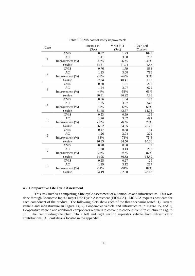
36
Table 10 CVIS control safety improvements
Case Mean TTC
(Sec) Mean PET
(Sec) Rear-End Crashes
CVIS 0.82 1.23 1028 AC 1.41 3.08 732
Improvement (%) -42% -60% -40% 1
t-value 44.51 41.94 1.86 CVIS 0.76 1.79 536 AC 1.23 3.08 796
Improvement (%) -38% -42% 33% 2
t-value 37.34 40.41 1.88 CVIS 0.70 1.51 268 AC 1.24 3.07 679
Improvement (%) -44% -51% 61% 3
t-value 30.81 36.22 7.36 CVIS 0.56 1.04 172 AC 1.25 3.07 549
Improvement (%) -55% -66% 69% 4
t-value 31.48 42.57 14.03 CVIS 0.53 0.99 109 AC 1.26 3.07 492
Improvement (%) -58% -68% 78% 5
t-value 26.62 34.85 26.26 CVIS 0.47 0.88 94 AC 1.26 3.04 372
Improvement (%) -63% -71% 75% 6
t-value 26.85 34.50 10.06 CVIS 0.28 0.30 37 AC 1.28 3.13 287
Improvement (%) -78% -90% 87% 7
t-value 24.95 56.62 18.50 CVIS 0.25 0.27 29 AC 1.29 3.12 217
Improvement (%) -81% -91% 87% 8
t-value 24.19 52.90 28.17
4.2. Comparative Life Cycle Assessment
This task involves completing a life cycle assessment of automobiles and infrastructure. This was done through Economic Input-Output Life Cycle Assessment (EIOLCA). EIOLCA requires cost data for each component of the product. The following plots show each of the three scenarios tested: 1) Current vehicle and infrastructure in Figure 14, 2) Cooperative vehicle and infrastructure in Figure 15, and 3) Cooperative vehicle and additional components required to convert to cooperative infrastructure in Figure 16. The bar dividing the chart into a left and right section separates vehicle from infrastructure contributions. All cost data is located in the appendix.
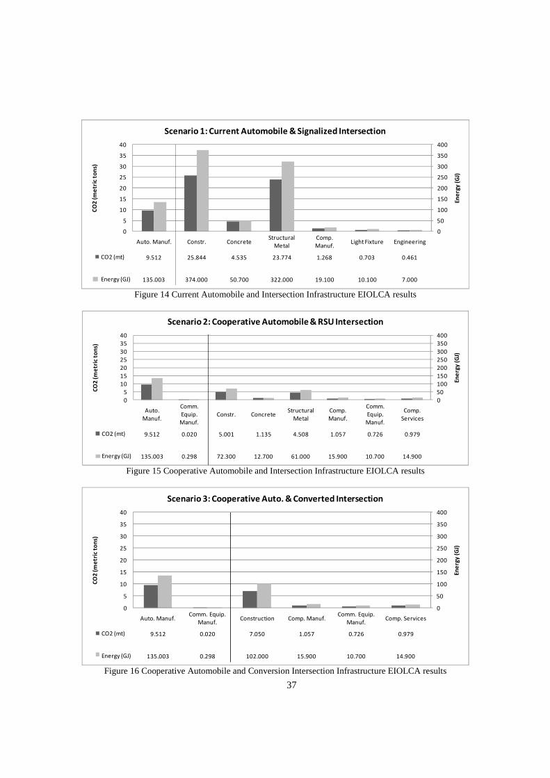
37
0
50
100
150
200
250
300
350
400
0
5
10
15
20
25
30
35
40
Auto. Manuf. Constr. ConcreteStructural
Metal
Comp.
Manuf.Light Fixture Engineering
CO2 (mt) 9.512 25.844 4.535 23.774 1.268 0.703 0.461
13.500 37.400 5.070 32.200 1.910 1.010 0.700
Energy (GJ) 135.003 374.000 50.700 322.000 19.100 10.100 7.000
En
erg
y (
GJ)
CO
2 (
me
tric
to
ns)
Scenario 1: Current Automobile & Signalized Intersection
Figure 14 Current Automobile and Intersection Infrastructure EIOLCA results
0
50
100
150
200
250
300
350
400
0
5
10
15
20
25
30
35
40
Auto.
Manuf.
Comm.
Equip.
Manuf.
Constr. ConcreteStructural
Metal
Comp.
Manuf.
Comm.
Equip.
Manuf.
Comp.
Services
CO2 (mt) 9.512 0.020 5.001 1.135 4.508 1.057 0.726 0.979
e as c 13.500 0.030 7.230 1.270 6.100 1.590 1.070 1.490
Energy (GJ) 135.003 0.298 72.300 12.700 61.000 15.900 10.700 14.900E
ne
rgy
(G
J)
CO
2 (
me
tric
to
ns)
Scenario 2: Cooperative Automobile & RSU Intersection
Figure 15 Cooperative Automobile and Intersection Infrastructure EIOLCA results
0
50
100
150
200
250
300
350
400
0
5
10
15
20
25
30
35
40
Auto. Manuf.Comm. Equip.
Manuf.Construction Comp. Manuf.
Comm. Equip.
Manuf.Comp. Services
CO2 (mt) 9.512 0.020 7.050 1.057 0.726 0.979
e as c 13.500 0.030 10.200 1.590 1.070 1.490
Energy (GJ) 135.003 0.298 102.000 15.900 10.700 14.900
En
erg
y (
GJ)
CO
2 (
me
tric
to
ns)
Scenario 3: Cooperative Auto. & Converted Intersection
Figure 16 Cooperative Automobile and Conversion Intersection Infrastructure EIOLCA results
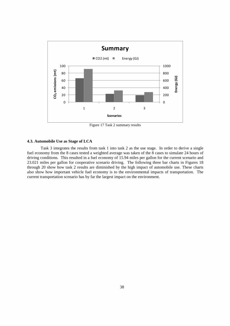
38
0
200
400
600
800
1000
0
20
40
60
80
100
1 2 3
Ene
rgy
(G
J)
CO
2e
mis
sio
ns
(mt)
Scenarios
Summary
CO2 (mt) Energy (GJ)
Figure 17 Task 2 summary results
4.3. Automobile Use as Stage of LCA
Task 3 integrates the results from task 1 into task 2 as the use stage. In order to derive a single fuel economy from the 8 cases tested a weighted average was taken of the 8 cases to simulate 24 hours of driving conditions. This resulted in a fuel economy of 15.94 miles per gallon for the current scenario and 23.021 miles per gallon for cooperative scenario driving. The following three bar charts in Figures 18 through 20 show how task 2 results are diminished by the high impact of automobile use. These charts also show how important vehicle fuel economy is to the environmental impacts of transportation. The current transportation scenario has by far the largest impact on the environment.
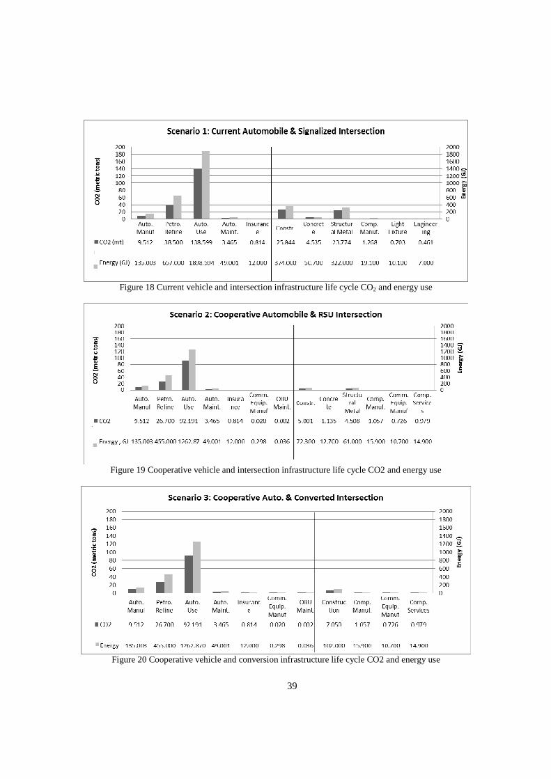
39
Figure 18 Current vehicle and intersection infrastructure life cycle CO2 and energy use
Figure 19 Cooperative vehicle and intersection infrastructure life cycle CO2 and energy use
Figure 20 Cooperative vehicle and conversion infrastructure life cycle CO2 and energy use
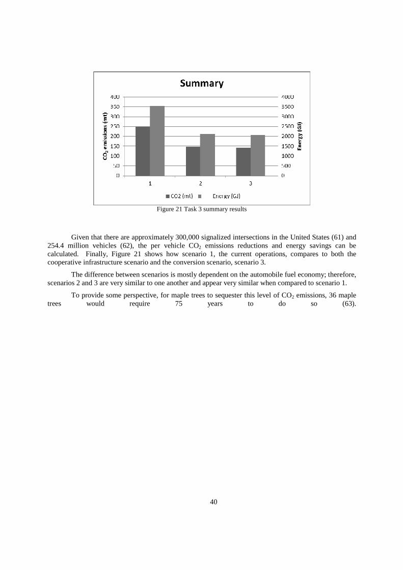
40
Figure 21 Task 3 summary results
Given that there are approximately 300,000 signalized intersections in the United States (61) and 254.4 million vehicles (62), the per vehicle CO2 emissions reductions and energy savings can be calculated. Finally, Figure 21 shows how scenario 1, the current operations, compares to both the cooperative infrastructure scenario and the conversion scenario, scenario 3.
The difference between scenarios is mostly dependent on the automobile fuel economy; therefore, scenarios 2 and 3 are very similar to one another and appear very similar when compared to scenario 1.
To provide some perspective, for maple trees to sequester this level of CO2 emissions, 36 maple trees would require 75 years to do so (63).
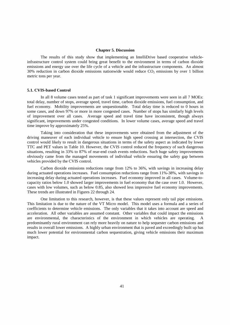
41
Chapter 5. Discussion
The results of this study show that implementing an IntelliDrive based cooperative vehicle-infrastructure control system could bring great benefit to the environment in terms of carbon dioxide emissions and energy use over the life cycle of a vehicle and the infrastructure components. An almost 30% reduction in carbon dioxide emissions nationwide would reduce CO2 emissions by over 1 billion metric tons per year.
5.1. CVIS-based Control
In all 8 volume cases tested as part of task 1 significant improvements were seen in all 7 MOEs: total delay, number of stops, average speed, travel time, carbon dioxide emissions, fuel consumption, and fuel economy. Mobility improvements are unquestionable. Total delay time is reduced to 0 hours in some cases, and down 97% or more in more congested cases. Number of stops has similarly high levels of improvement over all cases. Average speed and travel time have inconsistent, though always significant, improvements under congested conditions. In lower volume cases, average speed and travel time improve by approximately 25%.
Taking into consideration that these improvements were obtained from the adjustment of the driving maneuver of each individual vehicle to ensure high speed crossing at intersection, the CVIS control would likely to result in dangerous situations in terms of the safety aspect as indicated by lower TTC and PET values in Table 10. However, the CVIS control reduced the frequency of such dangerous situations, resulting in 33% to 87% of rear-end crash events reductions. Such huge safety improvements obviously came from the managed movements of individual vehicle ensuring the safety gap between vehicles provided by the CVIS control.
Carbon dioxide emissions reductions range from 12% to 36%, with savings in increasing delay during actuated operations increases. Fuel consumption reductions range from 11%-38%, with savings in increasing delay during actuated operations increases. Fuel economy improved in all cases. Volume-to-capacity ratios below 1.0 showed larger improvements in fuel economy that the case over 1.0. However, cases with low volumes, such as below 0.85, also showed less impressive fuel economy improvements. These trends are illustrated in Figures 22 through 24.
One limitation to this research, however, is that these values represent only tail pipe emissions. This limitation is due to the nature of the VT Micro model. This model uses a formula and a series of coefficients to determine vehicle emissions. The only variables that it takes into account are speed and acceleration. All other variables are assumed constant. Other variables that could impact the emissions are environmental, the characteristics of the environment in which vehicles are operating. A predominantly rural environment can rely more heavily on nature to help sequester carbon emissions and results in overall lower emissions. A highly urban environment that is paved and exceedingly built up has much lower potential for environmental carbon sequestration, giving vehicle emissions their maximum impact.
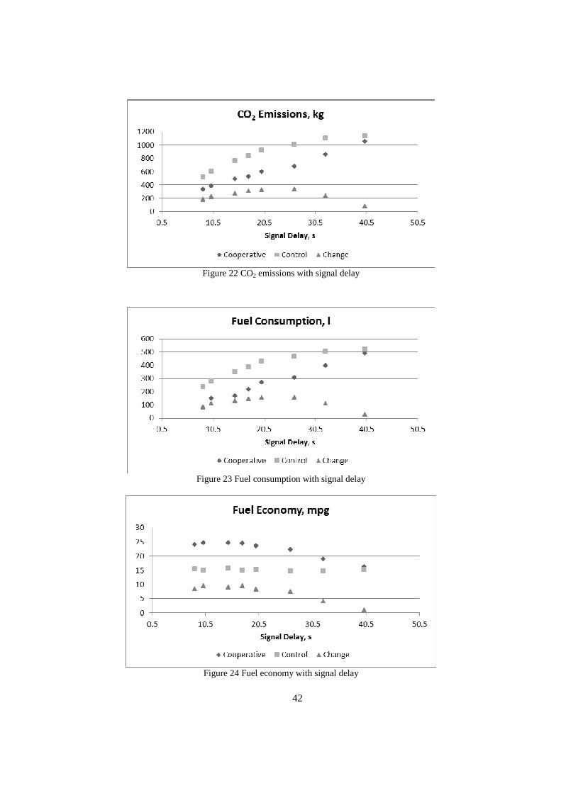
42
Figure 22 CO2 emissions with signal delay
Figure 23 Fuel consumption with signal delay
Figure 24 Fuel economy with signal delay
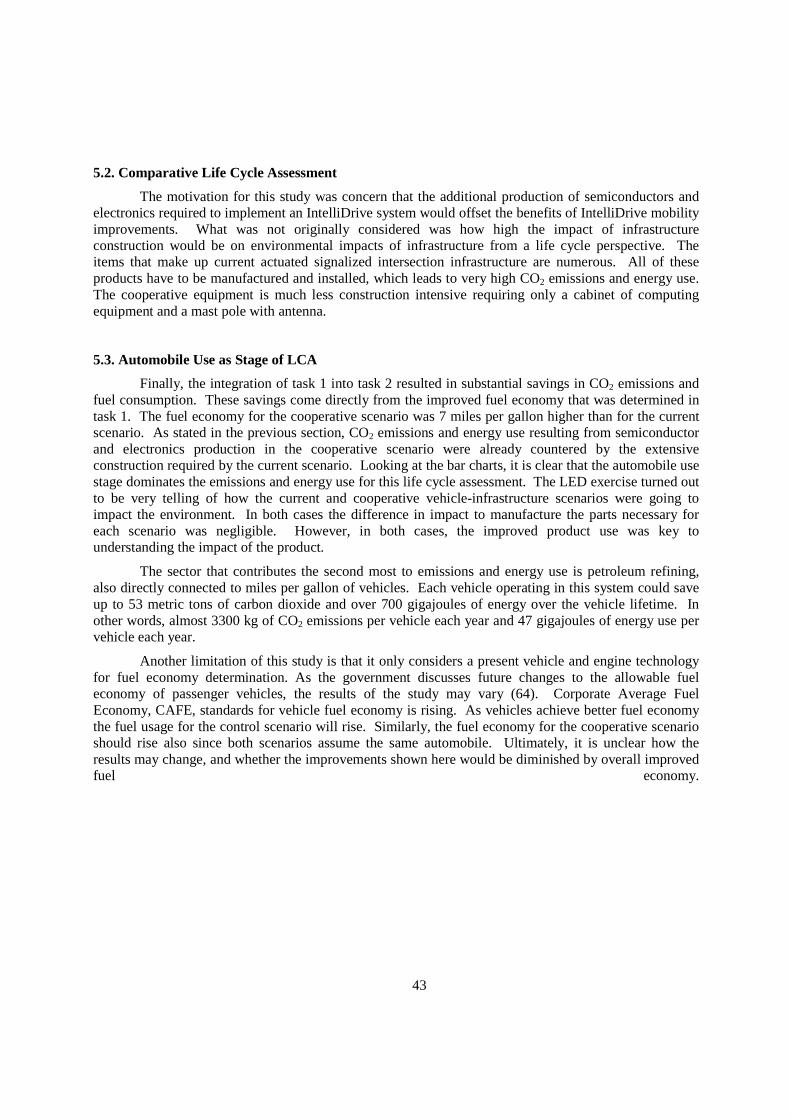
43
5.2. Comparative Life Cycle Assessment
The motivation for this study was concern that the additional production of semiconductors and electronics required to implement an IntelliDrive system would offset the benefits of IntelliDrive mobility improvements. What was not originally considered was how high the impact of infrastructure construction would be on environmental impacts of infrastructure from a life cycle perspective. The items that make up current actuated signalized intersection infrastructure are numerous. All of these products have to be manufactured and installed, which leads to very high CO2 emissions and energy use. The cooperative equipment is much less construction intensive requiring only a cabinet of computing equipment and a mast pole with antenna.
5.3. Automobile Use as Stage of LCA
Finally, the integration of task 1 into task 2 resulted in substantial savings in CO2 emissions and fuel consumption. These savings come directly from the improved fuel economy that was determined in task 1. The fuel economy for the cooperative scenario was 7 miles per gallon higher than for the current scenario. As stated in the previous section, CO2 emissions and energy use resulting from semiconductor and electronics production in the cooperative scenario were already countered by the extensive construction required by the current scenario. Looking at the bar charts, it is clear that the automobile use stage dominates the emissions and energy use for this life cycle assessment. The LED exercise turned out to be very telling of how the current and cooperative vehicle-infrastructure scenarios were going to impact the environment. In both cases the difference in impact to manufacture the parts necessary for each scenario was negligible. However, in both cases, the improved product use was key to understanding the impact of the product.
The sector that contributes the second most to emissions and energy use is petroleum refining, also directly connected to miles per gallon of vehicles. Each vehicle operating in this system could save up to 53 metric tons of carbon dioxide and over 700 gigajoules of energy over the vehicle lifetime. In other words, almost 3300 kg of CO2 emissions per vehicle each year and 47 gigajoules of energy use per vehicle each year.
Another limitation of this study is that it only considers a present vehicle and engine technology for fuel economy determination. As the government discusses future changes to the allowable fuel economy of passenger vehicles, the results of the study may vary (64). Corporate Average Fuel Economy, CAFE, standards for vehicle fuel economy is rising. As vehicles achieve better fuel economy the fuel usage for the control scenario will rise. Similarly, the fuel economy for the cooperative scenario should rise also since both scenarios assume the same automobile. Ultimately, it is unclear how the results may change, and whether the improvements shown here would be diminished by overall improved fuel economy.
44
Chapter 6. Conclusion and Recommendations
6.1 Conclusions
This research has shown the potential for IntelliDrive based cooperative vehicle-infrastructure control systems to improve the environmental impacts of transportation in the United States. As the number 2 sector in emissions of carbon dioxide from human related sources (3), the improvements shown here could seriously change how the sector is viewed and how the nation approaches issues of climate change and global warming.
This research examined the performances of mobility and sustainability and assessed the safety impacts of IntelliDrive-based urban traffic control system. The CVIS-based control algorithm under the IntelliDrive environment dramatically improved both the mobility and the environmental performances of the urban corridor.
Up to this point there is little clear evidence that IntelliDrive applications will provide the necessary change to achieve the “greener” goals that it has set for itself (4). Furthermore, there is limited research showing that IntelliDrive applications could improve intersection operations. This research shows that with mobility improvements on signalized intersections corridors, the environmental impacts of transportation will be reduced. The environmental improvements are directly related to the delay during actuated operations, higher delay allows for greater opportunity to improve operations. Marginal mobility improvements will provide marginal environmental improvements.
To further challenge the true environmental impacts of IntelliDrive based cooperative vehicle-infrastructure system technologies a life cycle assessment of the vehicle and infrastructure was conducted and showed that the two scenarios have similar infrastructure impacts, and that the automobile use stage governs the environmental impact. Few studies have used life cycle assessment to evaluate infrastructure. Typically, LCA is used to evaluate individual products, or alternative processes. This study budgeted an intersection construction project for each intersection, an actuated signal and a cooperative intersection. This information was then analyzed using economic input-output life cycle assessment. This method could very easily be utilized by practitioners who are looking to better understand the environmental impacts of comparable projects.
6.2 Recommendations
The report attempted many firsts for the field of transportation and while it has answered many questions, the results also pose many new questions that are recommended as future works. Generally speaking, this attempt as using life cycle assessment to help quantify environmental impacts of IntelliDrive technology successfully showed the high impacts that automobile use has on the environment. The transportation field should continue to pay special attention to environmental impacts because, as this study shows, seemingly small savings can contribute in a big way. Further exploration into the use of LCA and other environmental impacts tools in transportation is needed.
The first suggestion is that the cooperative vehicle-infrastructure test-bed used for this research continues to be expanded upon so that the improvement potential of this and other similar IntelliDrive applications can be better understood. This research added some features, but there are still more that could be added for more realistic driving simulation.
Another opportunity for future works on this report is to test the impact that this system would have on safety. As one of the three goals of the IntelliDrive program, safety is another important facet of transportation that could have a strong positive impact on society if it is improved. Though studies do suggest that safety could be improved, this has not been tested in an environment where the majority of vehicles are operating in a cooperative way.
45
A suggestion for future work that related more directly to the work done here is to improve the quantification of fuel economy. Fuel economy is made up of 55% city driving and 45% highway driving. This study quantifies a facet of city driving; however, it neglects highway driving. On a similar note, changing traffic characteristics such as speed limit may or may not change the resulting impacts to both mobility and environmental impact.
Another option for future works is to integrate process LCA into the analysis to create a hybrid approach. Hybrid LCA utilizes both Economic Input-Output LCA and process LCA to achieve a result that has some level of detail where it is needed and continues to use EIOLCA for areas that require less detail. A more detailed analysis of scenario 3 could improve the understanding of where emissions are derived from so informed decisions about how to implement IntelliDrive infrastructure can be made for the benefit of the environment.
Lastly, further research should focus on the environmental impacts of semiconductors and electronics. This study focuses on the greenhouse gas emissions and global warming impacts of semiconductor and electronics production and manufacturing. Though this is very important to society, other forms of pollution should not be over looked because those forms are just as important to society and need to be taken into consideration. Semiconductors require over 100 different material inputs, including lead, mercury, arsenic, and other carcinogens. If such metals and toxins are not properly cared for then the risk is that these metals enter the ground water and eventually the water supply that society is built upon. Research should be done to understand what impact mass production and disposal of RSU and OBU equipment could have on the environment in the future. Also, a plan for acquisition and proper reuse of these items after their perceived useful life is over should be considered.
Although there are some new questions that need to be answered, this research still clearly outlines some of the impressive greenhouse gas reducing benefits the IntelliDrive technology can have on transportation. CO2 emissions have been linked to global warming. By reducing CO2 emissions in the transportation sector by 30% dramatic change could be achieved without asking for dramatic changes by commuters. Finally, this research illustrates an application of life cycle assessment in transportation which could open new opportunities for transportation engineers to focus on environmental impacts when planning and making decisions regarding transportation infrastructure.
46
References
1. United Nations. "Millennium Development Goals Indicators."Carbon dioxide emissions (CO2) June 23, 2010 2010.Web. Carbon Dioxide Information Analysis Center. <http://mdgs.un.org/unsd/mdg/SeriesDetail.aspx?srid=749&crid=>.
2. U.S. Environmental Protection Agency. "EPA: Greenhouse Gases Threaten Public Health and the Environment."News Release issued by the Office of Air and Radiation. 12/7/2009 2009.Web.<http://yosemite.epa.gov/opa/admpress.nsf/7ebdf4d0b217978b852573590040443a/08d11a451131bca585257685005bf252!OpenDocument>.
3. U.S. Environmental Protection Agency. "Human Related Sources and Sinks of Carbon Dioxide." July 14 2010.Web. <http://www.epa.gov/climatechange/emissions/co2_human.html>.
4. IntelliDrive(Connected Vehicle Research). Available from: http://www.its.dot.gov/connected_vehicle /connected_vehicle.htm, Last Access: 2011.4.29
5. U.S. Department of Transportation. "AERIS: Applications for the Environment: Real-time Information Synthesis." IntelliDrive: Safer, Smarter, Greener. July 2010.Web. <http://www.intellidriveusa.org/research/aeris.php>.
6. Williams, E. D., R. U. Ayres, and M. Heller. "The 1.7 Kilogram Microchip: Energy and Material use in the Production of Semiconductor Devices."Environmental science & technology 36.24 (2002): 5504-10. Print.
7. Regenold, M. "The stop and Go! of traffic signals and their sometimes weird designs." Go! Exploring the World of Transportation. 2007.Web. <http://www.go-explore-trans.org/2007/may-jun/history_dept.cfm>.
8. Koonce, P., Rodergerdts, L., Lee, K., Signal Timing Manual. FHWA-HOP-08-024, Federal Highway Administration, Washington, DC. 2008.
9. Priemer, C., and B. Friedrich. "A Decentralized Adaptive Traffic Signal Control using V2I Communication Data". Intelligent Transportation Systems, 2009. ITSC '09. 12th International IEEE Conference on. 2009. 1-6. Print.
10. Federal Highway Administration. “The Exploratory Advanced Research Program Fact Sheet: Next-Generation Smart Traffic Signals RHODES with Intellidrive - the Self-Taught Traffic Control System (FHWA-HRT-09-063)” June 15, 2010. Web. http://www.fhwa.dot.gov/advancedresearch/pubs/NextGener.cfm. Accessed: November 2009.
11. Qi, Y., Chen, X., Yang, L. and Yu, L., Vehicle Infrastructure Integration (VII) Based Road-Condition Warning System For Highway Collision Prevention , Publication SWUTC/09/476660-00043-1, Southern Texas University Center for Transportation Training and Research, May 2009.
12. Wang, L. On Development of Intellidrive-based Red Light Running Collision Avoidance System. Richmond, CA: University of California, Berkeley, 3 4 2009.
13. Federal Motor Carrier Safety Administration. "Concept of Operations and Voluntary Operational Requirements for Forward Collision Warning Systems (CWS) and Adaptive Cruise Control (ACC) Systems On-board Commercial Motor Vehicles." July 2005. Forward Collision Warning System (CWS). 31 January 2010 <http://www.fmcsa.dot.gov/facts-research/research-technology/report/forward-collision-warning-systems.htm>.
47
14. Shladover, S.E., Effects of cooperative adaptive cruise control on traffic flow: testing drivers' choices of following distances. PATH Program Task Order 6202 UCS-ITS-PRR-2009-23, University of California Berkley, Berkeley, CA, 2009.
15. American Automobile Association Exchange. Winter Driving Tips. 2010.Web. <http://www.aaaexchange.com/main/default.asp?categoryid=3&subcategoryid=55>.
16. Shladover, S.E., Development and Evaluation of Selected Mobility Applications for VII. PATH Program Task Order 6224 UCS-ITS-PRR-2010-25, University of California Berkley, Berkeley, CA, 2009.
17. Arem van, B., C. J. G. Driel van, and R. Visser. "The Impact of Cooperative Adaptive Cruise Control on Traffic-Flow Characteristics." IEEE Transactions on Intelligent Transportation Systems 7.4 (2006): 429-436. Print.
18. Lee, J. Assessing the Potential Benefits of IntelliDrive-based Intersection Control Algorithms. Dissertation. University of Virginia December 2010.
19. S. Mandava, K. Boriboonsomsin, and M. Barth, “Arterial velocity planning based on traffic signal information under light traffic conditions” in Proc. of the 12th IEEE Intelligent Transportation Systems Conference, October 3-8, 2009, St. Louis, MO, USA
20. Energy Information Administration, Department of Energy. “Motor Gasoline Retail Prices” 2010. http://www.eia.gov/dnav/pet/pet_pri_top.asp. Accessed: October 2010.
21. Research and Innovative Technology Administration, Bureau of Transportation Statistics. “Table 1-38 - Principal Means of Transportation to Work”. National Transportation Statistics. 2010.
22. International Organization for Standardization. Environmental Management – Life Cycle Assessment – Principals and Framework. ISO 14040, 2006.
23. Hendrickson, C.T., L. B. Lave, and H.S. Matthews. Environmental Life Cycle Assessment of Goods and Services. Resources for the Future, Washington D.C., 2006.
24. SimaPro LCA Software. Product Ecology Consultants. http://www.pre.nl/simapro/. Accessed July, 2010.
25. Modular Open Source Software for Sustainability Assessment. The Open LCA Project. http://www.openlca.org/index.html. Accessed July 2010.
26. Gabi Software: Product sustainability. PE International. http://www.gabi-software.com/index.php?id=85&L=6&redirect=1. Accessed July 2010.
27. Swiss Centre for Life Cycle Inventories. "Ecoinvent Centre." 2010.Web. Ecoinvent v2.2. <http://www.ecoinvent.ch/>.
28. Leontief, W. Environmental repercussions and the economic structure: An input output approach. Review of Economics and Statistics, Vol. 52, No. 3, pp 262-271.
29. Economic Input-Output Life Cycle Assessment (EIO-LCA) US 1997 (491) model. Carnegie Mellon University. Green Design Institute. http://www.eiolca.net. Accessed July 2010.
30. CPI Inflation Calculator. Bureau of Labor Statistics. http://www.bls.gov/data/inflation_calculator.htm. Accessed July 2010.
31. Eco-LCA Ecologically-Based Life Cycle Assessment. The Ohio State University. The Center For Resilience. http://resilience.eng.ohio-state.edu/ecolca-cv/ Accessed July 2010.
32. Facanha, C. and A. Horvath, Environmental Assessment of Freight Transportation in the U.S.. International Journal of Life Cycle Assessment, Germany, Vol. 11 (4), 2006, pp. 229-239.
48
33. Weiss, M.A., J.B. Heywood, E.M. Drake, A. Schafer, and F.F. AuYeung. On the Road in 2020: A life-cycle analysis of new automobile technologies. MIT EL 00-003. Energy Laboratory, Massachusetts Institute of Technology, 2000.
34. Norman, J., H.L. MacLean, and C.A. Kennedy. Comparing High and Low Residential Density: Life-Cycle Analysis of Energy Use and Greenhouse Gas Emissions. ASCE Journal of Urban Planning and Development, March 2006, pp. 10-21.
35. Huang, Y., R. Bird, and M. Bell. A comparative study of the emissions by road maintenance works and the disrupted traffic using life cycle assessment and micro-simulation. Transportation Research Part D14, Transportation Research Board of the National Academies, Washington, D.C., 2009, pp. 197-204.
36. Zhou, Y., L. Tupper, M. Chowdhury, and L. Klotz. Green Credits vs. Environmentally Sustainable Traffic Operations: A Comparison of Contributions to Energy and Emissions Reductions [CD-ROM]. In Transportation Research Record: Journal of the Transportation Research Board, Transportation Research Board of the National Academies, Washington, D.C., 2010.
37. Soderlund, M., S.T. Muench, K.A. Willoughby, J.S. Uhlmeyer, and J.Weston. Green Roads: Sustainability Rating System for Roadways. TRB 87th Annual Meeting. CD-ROM. Transportation Research Board, Washington, D.C., 2007
38. PTV America. VISSIM Traffic Simulation. Version 5.10. (software). 2009 39. Mathworks, MATLAB&SIMULINK. 2009: MathWorks, Inc. Version R2008b. (software) 40. Husch, D., and Albeck., J. SYNCHRO 6 User Guide. Trafficware. 2004 41. Dowling, Richard, Alexander Skabardonis, and Vassili Alexiadis. Traffic Analysis Toolbox
Volume III: Guidelines for Applying Traffic Microsimulation Software. FHWA-HRT-04-040 Vol. Washington, D.C.: Federal Highway Administration, 2004. Web.
42. Gettman, D. and Head, L. Surrogate Measures of Safety from Traffic Simulation Models. Transportation Research Record: Journal of the Transportation Research Board. 1840: p. 104-115. 2003
43. Gettman, D. Pu, L., Sayed, T., and Shelb, S. Surrogate safety assessment model and validation: final report, Report No. FHWA-HRT-08-051. Federal Highway Administration (FHWA): Washington, D.C. 2008
44. Sylvania. How Halogen Works. 2010. <http://www.sylvania.com/ConsumerProducts/AutomotiveLighting/Products/Halogen/HowHalogenWorks.htm> Accessed August 2010.
45. Ron Goodin & Associates, Sales Representative Andy. Telephone Interview. 8 August 2010. 46. How Products are Made. Light Emitting Diode. 2010. <http://www.madehow.com/Volume-
1/Light-Emitting-Diode-LED.html> Accessed August 2010. 47. Urbank, Thomas, et al. LED Traffic Signal Monitoring, Maintenance, and Replacement Issues.
NCHRP Synthesis 387. Washington, D.C.: Federal Highway Administration, 2008. Web. 48. “Vehicle Traffic Control Signal Heads: Light Emitting Diode (LED) Circular Signal
Supplement,” Prepared by the Joint Industry and Traffic Engineering Council Committee, Institute of Transportation Engineers, Washington, D.C., June 27, 2005.
49. EP Lighting. Benefits of Krypton Incandescent Traffic Signal Lamps. 2010. <http://eplightingdivofepproducts.thomasnet.com/viewitems/incandescent-lamps/incandescent-krypton-traffic-signal-lamps> Accessed: August 2010.
49
50. GE Lumination. Full Ball. 2010. <http://www.lumination.com/literature/RX11_Full_Balls_8_and_12_inch_TRAF015_R022510_LR.pdf>. Accessed: August 2010.
51. U.S. Energy Information Administration. Energy Explained: Data & Statistics. 2010. http://www.eia.doe.gov/energyexplained/index.cfm?page=electricity_home#tab2. Accessed: September 2010.
52. Forster, P., V. Ramaswamy, P. Artaxo, T. Berntsen, R. Betts, D.W. Fahey, J. Haywood, J. Lean, D.C. Lowe, G. Myhre, J. Nganga, R. Prinn, G. Raga, M. Schulz and R. Van Dorland, 2007: Changes in Atmospheric Constituents and in Radiative Forcing. In: Climate Change 2007: The Physical Science Basis. Contribution of Working Group I to the Fourth Assessment Report of the Intergovernmental Panel on Climate Change [Solomon, S., D. Qin, M. Manning, Z. Chen, M. Marquis, K.B. Averyt, M.Tignor and H.L. Miller (eds.)]. Cambridge University Press, Cambridge, United Kingdom and New York, NY, USA.
53. Peirce, S., and R. Mauri. Vehicle-Infrastructure Integration (VII) Initiative Benefit-Cost Analysis: Pre- Testing Estimates: Draft Report. FHWA, U.S. Department of Transportation, RITA, March 30, 2007.
54. Sharafsaleh, A., J. VanderWerf, J. Misener, and S. Shladover. Implementing Vehicle Infrastructure Integration (VII): Real World Challenges. Intellimotion 14 (1), 2008, pp. 1-2, 4-7.
55. VDOT Bidtab Query. Virginia Department of Transportation. http://501stfs3/main/bridge/inside_vdot/bidtab_query.asp. Accessed July 2010.
56. Achieving the Vision: from VII to IntelliDrive. Reseach and Innovative Technology Administration. http://www.its.dot.gov/press/2010/vii2intellidrive.htm Accessed: December 2010.
57. Kelley Blue Book. Ford Taurus 2009. http://www.kbb.com/new-cars/ford/taurus/2009/pricing report#survey. Accessed July, 2010
58. Short Term Energy Outlook Custom Table Builder. Energy Information Administration, U.S. Department of Energy, 2010. http://www.eia.doe.gov/steo/cf_query/index.cfm. Accessed July, 2010
59. American Automobile Association. Your Driving Costs. Heathrow, FL, 2009. 60. Davis, S. C. and Diegel, S.W., Transportation Energy Data Book (22nd Ed.). Washington, DC:
U.S. Department of Energy, 2002. 61. Emission Facts: Greenhouse Gas Emissions from a Typical Passenger Vehicle. pollutants and
Programs. U.S. Environmental Protection Agency, Washington, D.C.. http://www.epa.gov/oms/climate/420f05004.htm. Accessed: July 2010.
62. Fuel Energy Comparisons: Gasoline Gallon Equivalents (GGE). Hybrid Cars and Alternative fuels. <http://alternativefuels.about.com/od/resources/a/gge.htm> Accessed August 2010.
63. Table 1-11: Number of U.S. Aircraft, Vehicles, Vessels, and Other Conveyances. National Transportation Statistics. Research and Innovative Technology Administration, Bureau of Transportation Statistics, 2010. http://www.bts.gov/publications/national_transportation_statistics/html/table_01_11.html. Accessed July, 2010.
64. Safety at Signalized Intersections. Federal Highway Administration, U.S. Department of Transportation. http://safety.fhwa.dot.gov/intersection/signalized/presentations/sign_int_pps051508/short/index.cfm. Accessed July, 2010.
65. How much does 1 tree offset?. Erase Carbon footprint. http://www.erasecarbonfootprint.com/treeoffset.html. Accessed July, 2010.
66. CAFE- Fuel Economy. National Highway Traffic Safety Administration. http://www.nhtsa.gov/fuel-economy. Accessed: December 2010.
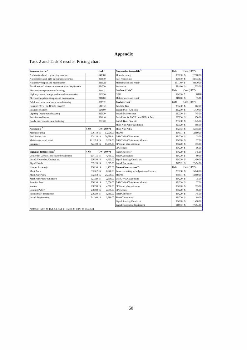
50
Appendix
Task 2 and Task 3 results: Pricing chart
Code Cooperative Automobile b Code Cost (1997)
Architectural and engineering services 541300 Manufacturing 336110 17,900.00$
Automobiles and light truck manufacturing 336110 Fuel Production 324110 18,473.63$
Automotive repair and maintenance 8111A0 Maintenance and repair 8111A0 9,630.00$
Broadcast and wireless communications equipment 334220 Insurance 524100 11,755.00$
Electronic computer manufacturing 334111 On-Board Unit d Code Cost (1997)
Highway, street, bridge, and tunnel construction 230230 OBU 334220 $ 80.00
Electronic equipment repair and maintenance 811200 Maintenance and repair 811200 13.00$
Fabricated structural metal manufacturing 332312 Roadside Unit e Code Cost (1997)
Computer Systems Design Services 541512 Junction Box 230230 662.00$
Insurance carriers 524100 Install: Mast Arm Pole 230230 1,470.00$
Lighting fixture manufacturing 335120 Install: Maintenance 230230 745.00$
Petroleum refineries 324110 Base Plate for MCNU and NEMA Box 230230 150.00$
Ready-mix concrete manufacturing 327320 Install: Base Plate etc 230230 1,045.00$
Mast Arm Pole Foundation 327320 588.00$
Automobile b Code Cost (1997) Mast Arm Poles 332312 6,473.00$
Manufacturing 336110 17,900.00$ MCNU 334111 3,680.00$
Fuel Production 324110 26,680.14$ DSRC/WAVE Antenna 334220 75.00$
Maintenance and repair 8111A0 9,630.00$ DSRC/WAVE Antenna Mounts 334220 37.00$
Insurance 524100 11,755.00$ GPS (unit plus antenna) 334220 373.00$
GPS Mount 334220 56.00$
Signalized Intersection c Code Cost (1997) Fiber Converter 334220 745.00$
Controller, Cabinet, and related equipment 334111 4,415.00$ Fiber Connectors 334220 89.00$
Install: Controller, Cabinet, etc 230230 4,415.00$ Signal Sensing Circuit, etc. 334220 1,490.00$
Signal Heads 335120 1,325.00$ Install Electronics 541512 7,454.00$
Hanger Assembly 230230 1,177.00$ Convert Intersection ce Code Cost (1997)
Mast Arms 332312 8,240.00$ Remove existing signal poles and heads 230230 5,740.00$
Mast Arm Poles 332312 25,900.00$ MCNU 334111 3,680.00$
Mast Arm Pole Foundation 327320 2,350.00$ DSRC/WAVE Antenna 334220 75.00$
Junction Box 230230 2,650.00$ DSRC/WAVE Antenna Mounts 334220 37.00$
saw cut 230230 4,560.00$ GPS (unit plus antenna) 334220 373.00$
Conduit PVC 1" 230230 2,355.00$ GPS Mount 334220 56.00$
Install: Mast arm & pole 230230 5,885.00$ Fiber Converter 334220 745.00$
Install: Engineering 541300 3,680.00$ Fiber Connectors 334220 89.00$
Signal Sensing Circuit, etc. 334220 1,490.00$
Install:Computing Equipment 541512 7,454.00$
Economic Sector a
Note: a: (28); b: (53, 54, 55); c: (53); d: (50); e: (50, 51)