Quantification of Geometric Uncertainties in Image Guided...

Quantification of Geometric Uncertainties in Image Guided

Radiotherapy

Investigation of geometric uncertainties, automatic image registration performance

and quality metrics for image registration applied to the Elekta Synergy® cone

beam computed tomography based image guided radiotherapy system

Jonathan Rolf Sykes

Submitted in accordance with the requirements for the degree of

Doctor of Philosophy

The University of Leeds

(1) Leeds Institute of Genetics, Health and Therapeutics,

School of Medicine and

(2) School of Computing

October, 2010

2

This copy has been supplied on the understanding that it is copyright material and

that no quotation from the thesis may be published without proper acknowledgement.

The right of Jonathan Rolf Sykes to be identified as Author of this work has been

asserted by him in accordance with the Copyright, Designs and Patents Act 1988.

© 2010 The University of Leeds and Jonathan Rolf Sykes

3

Declarations

The candidate confirms that the work submitted is his/her own, except where work

which has formed part of jointly-authored publications has been included. The

contribution of the candidate and the other authors to this work has been explicitly

indicated below. The candidate confirms that appropriate credit has been given within

the thesis where reference has been made to the work of others.

The following jointly-authored publications are based on the work of Chapters 3

and 6 respectively.

1. Sykes, JR, Lindsay, R, Dean, CJ, Brettle, DS, Magee, DR, Thwaites, DI.

Measurement of cone beam CT coincidence with megavoltage isocentre

and image sharpness using the QUASAR™ Penta-Guide phantom. Phys

Med Biol 2008;53:5275-5293.

2. Sykes, JR, Brettle, DS, Magee, DR, Thwaites, DI. Investigation of

uncertainties in image registration of cone beam CT to CT on an image-

guided radiotherapy system. Phys Med Biol 2009;54:7263-7283.

In both cases the work originated from intellectual property generated by, the

candidate and the majority of measurements were performed by the candidate. All data

was analysed and the articles were written by the candidate as primary author. The

authors, R. Lindsay, and C.J. Dean performed some of the measurements presented in

chapter 3 under the supervision of the candidate. The authors D.R. Magee, D.S. Brettle

and D.I. Thwaites are the candidate's supervisors and their input was that of a normal

student-supervisor relationship.

4

This research work and publications and presentations arising from it were

supported by the award of an IPEM Research Fellowship (2005 – 2009)

Relevant abstracts based on, or in-part, work presented in this thesis

[1] Naisbit M, Sykes JR, Brettle DS, Magee DR, Thwaites DI. A Technique For

Measuring Translation And Rotation Positioning Accuracy Of Automatic Table

Movements Using Cone Beam CT. Radiotherapy and Oncology

2010;96(Supplement 1):S523.

[2] Lindsay R, Sykes JR, Stanley S, Dickinson R, Thwaites DI. A technical

evaluation and implementation survey of three IGRT systems at eleven UK

centres. 10th Biennial ESTRO Physics 2009, Maastricht.

[3] Sykes JR. Review of Current IGRT Research - Dosimetry Perspective. 10th

Biennial ESTRO Physics 2009, Maastricht.

[4] Sykes JR, Lindsay R, Fairfoul J, Emmens D, Dickinson R, Thwaites DI.

Development of a clinically realistic test for evaluation of X-ray tomographic

IGRT systems. 10th Biennial ESTRO Physics 2009, Maastricht.

[5] Lindsay R, Sykes J, Thwaites DI. Development of a national protocol for

evaluating the performance of X-ray volumetric IGRT systems. ESTRO 27 2008,

Goteborg, Sweden: S45.

[6] Lindsay R, Sykes JR, Stanley S, Thwaites DI, Dickinson R. An evaluation of

tomographic IGRT technologies. Institute of Physics and Engineering in

Medicine Biennial Radiotherapy Meeting 2008, Bath, UK: 89.

[7] Sykes J. Geometric QA of IGRT systems. ESTRO 27 2008, Goteborg, Sweden:

S171.

[8] Sykes J, Brettle DS, Magee DR, Morgan AM, Thwaites DI. A software tool to

adapt the QUASAR™ Penta-Guide phantom to make an additional measurement

of cone beam CT image sharpness. AAPM annual Meeting 2008, Houston,

Texas, US: 2778.

5

[9] Sykes J, Lindsay R, Brettle DS, Magee DR, Thwaites DI. Development and

evaluation of a method to improve accuracy of cone beam CT to MV isocentre

image alignment using the QUASAR™ Penta-Guide phantom. ESTRO 27 2008,

Goteborg, Sweden: S370.

[10] Sykes JR, Lindsay R, Dean CJ, Brettle DS, Magee DR, Thwaites DI. Quality

assurance of cone beam CT based IGRT systems using the Penta-Guide phantom.

Institute of Physics and Engineering in Medicine Biennial Radiotherapy Meeting

2008, Bath, UK: 89.

[11] Sykes JR, Morgan AM, Brettle DS, Magee D, Thwaites DI ’Measurement of cone

beam CT image registration error with a skull phantom for image guided

radiotherapy and its relationship with imaging dose’, 9th Bienneal ESTRO meeting

on Physics and Radiation Technology for Clinical Radiotherapy,

Radiother.Oncol.2007, 84 (Suppl 1)

6

Acknowledgements

I would like to express my deepest gratitude to all my supervisors, Derek Magee,

David Brettle and David Thwaites throughout the five year duration of this research

degree. Between them, they provided a good balance of expertise, guidance, support

and encouragement and have helped me to further develop my research skills.

I would like to thank the Institute for Physics and Engineering in Medicine for the

award of the IPEM research fellowship which funded me part time through the first four

years of my studies. I would also like to recognise the support of my colleagues in the

Radiotherapy physics group of the Medical Physics and Engineering department at

Leeds Teaching Hospitals Trust who have supported me in some of my clinical duties

and enabled me to dedicate sufficient time to my studies. In particular, I am grateful to

Christopher Dean, Rebecca Lindsay and Mitchell Naisbit who helped measure some of

the data.

I would like to thank Elekta for providing a license of the Synergy® XVI software

for research purposes and Marcel Van Herk and the team at the Netherlands Cancer

Institute for providing a research version of the XVI software with the extra

functionality required to perform the last chapter of this thesis.

I am grateful to my parents who ensured I had a good educational start in life but

in particular to my father, Dr Alan Sykes, who, as a retired lecturer in statistics, has

pointed me towards appropriate statistical methods in the analysis of my data.

Finally, I am tremendously grateful to my wife Bridget, who has supported my

studies in many ways; not least by taking on more than her fair share of managing the

household and bringing up my daughter Hannah and son Daniel who were both born

within the duration of this project.

7

Abstract

The aim of this thesis is to determine if the geometric uncertainties that are

introduced into the image guided radiotherapy (IGRT) process by Cone Beam CT

(CBCT) based IGRT equipment are sufficiently small that they do not pose a significant

risk of geometrical error in treatment delivery. This was performed by quantifying and

investigating the geometric uncertainties introduced by; (1) calibration of the image

geometry, (2) correction of patient position performed by automatic treatment couch

systems and (3) automatic image registration of the localisation image with a reference

image. In addition, the feasibility of providing user feedback on the likelihood of

accurate image registration was investigated. A method was developed using

supervised machine learning based on the shape of the image registration algorithm's

similarity metric surface.

The geometric uncertainties introduced by image calibration and couch positioning

were both shown to be less than 1 mm and therefore do not contribute significantly to

the overall uncertainties in the IGRT process. Image registration performance for image

guidance based on the bony anatomy of the skull was shown to be reproducible, accurate

and robust with errors typically less than 1 mm. Moreover, image registration

performance did not deteriorate significantly as imaging dose was reduced. For image

guidance based on the soft tissues of the prostate, image registration performance was

satisfactory for some CBCT images resulting in errors less than 2 mm. However, with

the majority of CBCT images, image registration was highly irreproducible with high

frequencies of failure. The user feedback of image registration quality was able to

correctly classify 84% of image registrations into categories of good, acceptable and

unacceptable. No unacceptable classifications were classed as good.

CBCT based IGRT equipment does not introduce significant risks into the IGRT

process however, appropriate quality assurance measures should be implemented to

safeguard against equipment failure and drift since previous system calibration.

Automatic image registration of the soft-tissues of the prostate cannot be relied upon for

clinical use and therefore it should be used in conjunction with manual methods.

8

Contents

Declarations .......................................................................................................... 2

Acknowledgements.................................................................................................... 6

Abstract .......................................................................................................... 7

Contents .......................................................................................................... 8

List of Figures ........................................................................................................ 15

List of Tables ........................................................................................................ 18

Glossary ........................................................................................................ 20

Chapter 1 Introduction.................................................................................. 24

1.1 Brief Introduction to Image Guided Radiotherapy.................................. 24

1.2 Motivation............................................................................................... 27

1.3 Hypothesis and research questions.......................................................... 30

1.4 Overview................................................................................................. 31

Chapter 2 Background................................................................................... 34

2.1 Introduction to image guided radiotherapy (IGRT) ................................ 34

2.1.1 Introduction to radiotherapy........................................................... 34

2.1.2 The role of imaging in radiotherapy............................................... 36

2.1.3 Image guided radiotherapy............................................................. 37

2.1.4 IGRT research topics...................................................................... 38

2.2 Geometric uncertainties in image guided radiotherapy........................... 40

2.2.1 Introduction to geometric uncertainties in radiotherapy ................ 40

2.2.2 Managing risk in radiotherapy ....................................................... 41

2.2.3 Sources of geometric accuracy in CBCT imaging systems............ 41

2.2.4 Calibrating image geometry in CBCT imaging systems................ 46

2.3 Quality assurance/commissioning measurements for CBCT based

IGRT equipment...................................................................................... 47

2.3.1 Measurement of kV-MV alignment in CBCT systems.................. 49

2.3.2 Accuracy and precision of automatic couch positioning in IGRT

systems ........................................................................................... 52

2.3.3 Measurement of image scaling and distortion................................ 55

2.3.4 Measurement of image resolution/sharpness ................................. 57

2.3.5 Combined geometric and dosimetric accuracy measurements....... 58

9

2.4 Automated image registration performance evaluation and associated

geometric uncertainties ........................................................................... 58

2.4.1 Introduction to automated image registration ................................ 58

2.4.2 Image registration algorithms used in the Elekta Synergy® IGRT

system............................................................................................. 60

2.4.3 Image registration performance, accuracy, precision and quality

assurance ........................................................................................ 63

2.4.3.1 Evaluation of accuracy by hidden markers ..................... 64

2.4.3.2 Evaluation of image registration consistency.................. 65

2.4.3.3 Visual assessment............................................................ 66

2.4.3.4 Alternative methods ........................................................ 67

2.4.4 Performance evaluation of commercial image registration

algorithms....................................................................................... 67

2.4.5 Relationship between image quality (dose) and image registration

performance.................................................................................... 69

2.4.6 Methods for checking image registration quality (user feedback) . 71

2.5 Introduction to tools used in the thesis.................................................... 72

2.5.1 Measurement of image sharpness .................................................. 72

2.5.2 Dual quaternions to represent rigid body transformations ............. 76

2.5.3 Evaluation of image registration similarity metrics ....................... 77

2.5.4 Supervised Machine learning (Data mining) ................................. 78

2.6 Summary ................................................................................................. 80

Chapter 3 Quantification of misalignments in cone beam CT based

IGRT equipment ............................................................................................ 81

3.1 Introduction ............................................................................................. 81

3.2 Background ............................................................................................. 82

3.3 Methods................................................................................................... 86

3.3.1 CBCT-MV isocentre alignment using the ball bearing phantom... 86

3.3.2 Daily check of flat panel imager alignment ................................... 89

3.3.3 Measurement of CBCT-MV isocentre alignment using the Penta-

Guide phantom............................................................................... 89

3.3.3.1 MV radiation field centre localisation............................. 90

3.3.3.2 Penta-Guide air cavity centre localisation using MV

images ................................................................................... 94

3.3.3.3 Back projection ............................................................... 94

10

3.3.3.4 XVI centre to air-cavity centre alignment using the

Penta-Guide phantom............................................................ 95

3.3.3.5 Repeatability, reproducibility and comparative tests ...... 96

3.3.4 Method for approximating the image sharpness from CBCT

scans of the Penta-Guide phantom................................................. 96

3.3.4.1 Locating the centre of air cavity...................................... 97

3.3.4.2 Extracting profiles........................................................... 98

3.3.4.3 Fitting the edge response function ................................ 100

3.3.4.4 Repeatability of MTF50 calculation and sensitivity of

MTF50 to panel misalignment ............................................. 102

3.4 Results................................................................................................... 103

3.4.1 CBCT-MV isocentre measurements using the Ball Bearing

phantom........................................................................................ 103

3.4.2 Daily check of panel position....................................................... 105

3.4.3 CBCT-MV isocentre alignment repeatability and comparative

tests............................................................................................... 106

3.4.4 MTF50 calculation from Penta-Guide Phantom ........................... 108

3.5 Discussion ............................................................................................. 113

3.6 Conclusions and Future Work............................................................... 117

3.6.1 Conclusion ................................................................................... 117

3.6.2 Future Work ................................................................................. 118

Chapter 4 Target Registration Error ......................................................... 120

4.1 Introduction ........................................................................................... 120

4.2 Target registration error calculated from mean displacement of points

on sphere ............................................................................................... 121

4.3 Discussion ............................................................................................. 122

Chapter 5 Measurement of automatic patient support movement

accuracy ...................................................................................................... 125

5.1 Introduction ........................................................................................... 125

5.2 Materials and Methods.......................................................................... 127

5.2.1 Preparation of reference FBCT data............................................. 128

5.2.2 Image guidance Procedure ........................................................... 130

5.2.3 Study details ................................................................................. 131

5.2.4 Cross registration of images......................................................... 132

5.3 Results................................................................................................... 134

5.4 Discussion ............................................................................................. 141

11

5.5 Conclusion and future work .................................................................. 144

5.5.1 Conclusions.................................................................................. 144

5.5.2 Future Work ................................................................................. 144

Chapter 6 Measurement of automatic image registration uncertainties

for intra-cranial tumours: skull phantom and patient CT and CBCT

images ...................................................................................................... 145

6.1 Introduction ........................................................................................... 145


6.2.1 Measurement of registration uncertainty...................................... 149

6.2.2 Skull phantom studies .................................................................. 150

6.2.2.1 FBCT of skull phantom................................................. 150

6.2.2.2 Study I, registration performance with imaging dose

(skull phantom) ................................................................... 151

6.2.2.3 Study II, registration performance with image resolution

(skull phantom) ................................................................... 155

6.2.3 Patient Studies.............................................................................. 155

6.2.3.1 Study III, registration performance with patient images157

6.2.3.2 Study IV, Registration uncertainty with clipbox position

(patient images)................................................................... 157

6.2.3.3 Study V, Registration performance after multiple image

registrations (patient images) .............................................. 157

6.2.3.4 Study VI, Registration performance with the 'Elekta

Correlation Ratio' algorithm (patient images)..................... 158

6.2.3.5 Study VII, Effect of image re-sampling (patient images)158

6.2.4 Image registration error analysis .................................................. 158

6.2.5 Measurement of dose ................................................................... 161

6.3 Results................................................................................................... 161

6.3.1 Study I, Registration performance with imaging dose (skull

phantom) ...................................................................................... 161

6.3.2 Study II, Registration performance with image resolution (skull

phantom) ...................................................................................... 165

6.3.3 Study III, registration performance with patient images .............. 166

6.3.4 Study IV, Registration uncertainty with clipbox position (patient

images) ......................................................................................... 168

6.3.5 Study V, Registration performance after multiple image

registrations (patient images) ....................................................... 172

12

6.3.6 Study VI, Registration performance with the grey value matching

algorithm (patient images) ........................................................... 172

6.3.7 Study VII, Effect of image re-sampling (patient images)............. 173

6.4 Discussion ............................................................................................. 176

6.5 Conclusions and Future Work............................................................... 181

6.5.1 Conclusions.................................................................................. 181

6.5.2 Future Work ................................................................................. 182

Chapter 7 Measurement of automatic image registration uncertainties

for prostate tumours: pelvis phantom and patient FBCT and CBCT

images ...................................................................................................... 183

7.1 Introduction ........................................................................................... 183


7.2.1 FBCT and CBCT imaging............................................................ 185

7.2.1.1 Phantom Imaging .......................................................... 185

7.2.1.2 Patient Imaging ............................................................. 186

7.2.2 Image Registrations...................................................................... 186

7.3 Results................................................................................................... 188

7.4 Discussion ............................................................................................. 193

7.5 Conclusion ............................................................................................ 195

7.6 Future work ........................................................................................... 195

Chapter 8 Image registration quality likelihood metrics based on

similarity metric surface shape ................................................................... 197

8.1 Introduction ........................................................................................... 197


8.2.1 Phantom and patient data ............................................................. 199

8.2.2 Sampling the similarity metric ..................................................... 199

8.2.2.1 Pre-release XVI v4.5 research mode............................. 199

8.2.2.2 Sampling of the rigid body transform parameter space. 199

8.2.2.3 Sub-sampling registration uncertainty datasets based on

TRE50 value......................................................................... 200

8.2.2.4 Calculation of similarity metric samples....................... 200

8.2.3 Evaluation of similarity metric profiles ....................................... 201

8.2.4 Classification of image registration quality.................................. 202

8.2.5 Sub-sampling of parameter space (calculation at 25 points)........ 203

8.3 Results................................................................................................... 205

13

8.3.1 Registration Uncertainties............................................................ 205

8.3.2 Correlation Ratio Similarity Metric Profiles................................ 208

8.3.3 Classification results .................................................................... 210

8.4 Discussion ............................................................................................. 214

8.5 Conclusion ............................................................................................ 217

8.6 Future work ........................................................................................... 218

Chapter 9 Conclusions and future work.................................................... 219

9.1 Conclusions........................................................................................... 219

9.1.1 Chapter 3 - Quantification of misalignments in cone beam CT

based IGRT equipment................................................................. 220

9.1.2 Chapter 4 - Target Registration Error .......................................... 222

9.1.3 Chapter 5 - Measurement of automatic patient support movement

accuracy........................................................................................ 222

9.1.4 Chapters 6 and 7 - Measurement of automatic image registration

uncertainties for intra-cranial and prostate tumours..................... 223

9.1.5 Chapter 8 - Image registration quality likelihood metrics based

on similarity metric surface shape................................................ 225

9.2 Future Work .......................................................................................... 225

9.3 Impact and novel contributions............................................................. 228

References ...................................................................................................... 219

Appendix A Rigid body transformations: notation and conversion ................ 246

A.1 Introduction ........................................................................................... 246

A.2 Rigid body transforms represented by Euler Angles as used by the

Synergy® XVI software........................................................................ 247

A.3 Rigid body transforms represented by Euler parameters or Versors as

used by ITK...........................................................................................248

A.4 Rigid body transforms represented by Dual Quaternions ..................... 249

A.5 Calculating the mean of multiple rigid body transforms....................... 252

A.6 Calculating the error transform ............................................................. 253

A.7 Conversion between Synergy® transform parameters, ITK Versor

parameters and Dual Quaternions ......................................................... 254

14

Appendix B Metrics for evaluation of similarity measure rigid body

parameter space............................................................................................ 264

B.1 Metrics for evaluation of similarity measure profiles ........................... 264

B.1.1 Accuracy (ACC)........................................................................... 265

B.1.2 Risk of non-convergence (RON).................................................. 265

B.1.3 Distinctiveness of optimum (DO) ................................................ 266

B.2 Metrics for evaluation of sub-sampled (25 point) similarity metric

profiles................................................................................................... 267

B.2.1 Distinctiveness of Optimum DO25(1), DO25(2) & DO25(Av) ...... 267

B.2.2 Minimum Value, ∆Xmin,25............................................................ 268

B.3 Quadratic fit to calculate ∆X25,fit and SM25(X25,fit) ............................... 268

15

List of Figures

Figure 1. One of the Elekta Synergy® systems at St James's Institute for

Oncology. ........................................................................................................ 26

Figure 2. Illustration of cone CT beam system geometry and possible

misalignments ................................................................................................. 43

Figure 3. Illustration of edge spread function derived from an inclined edge. . 74

Figure 4. The Penta-Guide phantom.....................................................................85

Figure 5. Diagram of Elekta Synergy® system and its geometry for each field

of view. ........................................................................................................ 88

Figure 6. MV portal image of the Penta-Guide phantom zoomed in on the

radiation field. ................................................................................................ 91

Figure 7. Frequency distribution of the pixel intensity values in the MV

portal image. ................................................................................................... 92

Figure 8. Illustration of the linear Hough transform........................................... 93

Figure 9. MV portal image of air-cavity in Penta-Guide phantom. ................... 95

Figure 10. Effect of CBCT panel alignment on sharpness of Penta-Guide

phantom air cavity. ........................................................................................ 99

Figure 11. Illustration of the spherical air-cavity and four conical sections. .. 100

Figure 12. (a) Example of a radial profile along a collapsed cone with the

error function fit and (b) corresponding MTF curve. .............................. 102

Figure 13. Results of daily alignment checks...................................................... 106

Figure 14. MTF50 calculated for radial angles in the central axial plane of a

CBCT scan of the Penta-Guide phantom using the edge response

function of the air cavity.............................................................................. 109

Figure 15. Variation of MTF50 measured in the axial plane on repeat scans 1-

5 of the Penta-Guide phantom (Penta-Guide (1-5) in legend).................. 111

Figure 16. Variation of MTF50 measured along the longitudinal axis on

repeat scans 1-5 of the Penta-Guide phantom (Penta-Guide (1-5) in

legend). ...................................................................................................... 112

Figure 17. Illustration of sphere triangulated into 643 equi-spaced vertices

and calculation of TRE50,max........................................................................ 123

Figure 18. Sections through the FBCT scan of the VHMP phantom............... 129

16

Figure 19. Diagram illustrating the 5 reference CT scans (RefT0 to RefT4), the

six phantom positions (PosT0 to PosT5) at which CBCT images were

acquired and the 30 possible combinations of FBCT and CBCT scan

pairs for which image registration was performed................................... 133

Figure 20. Rigid body position/image registration errors for the six studies

represented by TRE50 .................................................................................. 136

Figure 21. Residual errors having removed the mean couch positioning error

for studies,..................................................................................................... 137

Figure 22. Trans-axial slices through the centre of the CBCT scans of the

skull phantom............................................................................................... 156

Figure 23. Registration performance for Study Ii .............................................. 162

Figure 24. Registration performance for Study Iii ............................................. 163

Figure 25. Registration performance for Study Iiii ............................................ 164

Figure 26. Registration performance for Study Iiv............................................. 165

Figure 27. Registration performance for Study II.............................................. 167

Figure 28. Registration performance for Study III ............................................ 169

Figure 29. Study III, Plot of measured registration error, ( )i50 eTRE δ against

applied misalignment, InitialTRE for all patient data................................... 170

Figure 30. Registration performance for Study IV............................................. 171

Figure 31. Registration performance for Studies V, VI & VII........................... 174

Figure 32. Correlation between registration uncertainties for Studies V, VI &

VII ...................................................................................................... 175

Figure 33. Transaxial, Sagittal and Coronal sections through CBCT scan A

scanned with the highest dose setting......................................................... 188

Figure 34. Transaxial sections of CBCT scans A to G, centred on the

prostate, showing the deterioration of image quality with imaging dose.189

Figure 35. Soft tissue registration performance for VHMP phantom with

decreasing dose. ............................................................................................ 191

Figure 36. Soft tissue registration performance for the prostate in patient

images. ...................................................................................................... 192

Figure 37. Registration performance for patient head images with the

research Synergy XVI v4.5 and the Chamfer matching similarity

metric. ...................................................................................................... 206

Figure 38. Registration performance for patient head images with the

research Synergy XVI v4.5 and the Correlation Ratio similarity metric.207

17

Figure 39. Examples of correlation ratio SM profiles along the three

translation and three rotation axis with increasing TRE50, for one

patient. ...................................................................................................... 208

Figure 40. Examples of correlation ratio SM profiles along the three

translation and three rotation axis with increasing TRE50, for one

patient. ...................................................................................................... 209

Figure 41. Correlation ratio similarity metric prof iles centred on the mean

image registration transform (TRE50 = 0) with the first FBCT-CBCT

image pair of each patient. .......................................................................... 210

Figure 42. Correlation ratio similarity metric prof iles centred on the mean

image registration transform (TRE50 = 0) for the first three FBCT-

CBCT image pairs of patient 1. .................................................................. 211

Figure 43. The IEC 1217 coordinate system as applied to the Elekta

Synergy® system. Picture taken from the Elekta Synergy®, Clinical

Mode User Manual for XVI R4.2 ............................................................... 248

Figure 44. Diagram to show a) calculation of image registration error from

measured and applied transforms, b) calculation of mean error

transform and c) calculation of residual image registration error.......... 253

Figure 45. Examples of the quadratic fit to the similarity metric profiles....... 270

18

List of Tables

Table 1. MV isocentre position, difference between MV isocentre and BB

position and difference between CBCT image centre and MV isocentre105

Table 2. Mean and standard deviation of residuals for MV isocentre and

CBCT-MV alignment using both the ball bearing and Penta-Guide

methods. ...................................................................................................... 107

Table 3. Study parameters used in studies 1-12. ................................................ 131

Table 4. Median, maximum and standard deviation of the TRE50 (mm) for

the raw error, group mean error and residual error for each study....... 138

Table 5. Mean, standard deviation (SD), maximum absolute (Max ABS) and

mean absolute (Accuracy) translation and rotation error parameters for

each of the studies. ....................................................................................... 140

Table 6. Mean, standard deviation (SD), maximum absolute (Max ABS) and

mean absolute (Accuracy) translation and rotation error parameters. .. 141

Table 7. Exposure settings for CBCT scans acquired for study Ii ................... 152

Table 8. Exposure settings for CBCT scans acquired for study Iii .................. 153

Table 9. Settings for CBCT scans reconstructed from CBCT scan A3 for

study Iiii ...................................................................................................... 154

Table 10. Settings for CBCT scans reconstructed from CBCT scan B4 for

study Iiv ...................................................................................................... 154

Table 11. Exposure settings for the seven scans A-G and a measurement of

nominal scan dose measured in a CTDI phantom with a Farmer

chamber. ...................................................................................................... 186

Table 12. Confusion table showing classification of TRE50 values using a

Bayesian network based on the similarity metric full profile evaluation

metrics for image registrations performed using the correlation ratio... 212


Bayesian network based on the similarity metric 25 point evaluation

metrics for image registrations performed using the correlation ratio... 212


Bayesian network based on the similarity metric full profile evaluation

metrics for image registrations performed using the chamfer match. .... 213

19


Bayesian network based on the similarity metric 25 point evaluation

metrics for image registrations performed using the chamfer match. .... 213

Table 16. Dual number algebra. .......................................................................... 250

Table 17. Dual quaternion algebra...................................................................... 251

Table 18. Representation of rigid body transforms using unit dual

quaternions. .................................................................................................. 252

Table 19. Table of ITK VersorRigid3DTransform rigid body transform

parameters used to establish correspondence between ITK and

Synergy® parameters. Translations t1-t3 are in units of mm while a

Versor value (q1-q3) of 0.0872 is equivalent to 10°................................... 255

Table 20. Results of image registration in Synergy® format of localisation

CBCT image in the reference position against transformed reference

CT datasets 1a-1j.......................................................................................... 256

Table 21. Correspondence between Synergy® and ITK

VersorRigid3DTransform parameters....................................................... 257

Table 22. Residual errors between measured and applied transforms in

versor notation when the reference CT image is transformed and the

localisation CBCT is of the phantom in its reference position................. 260

Table 23. Residual errors between measured and applied transforms in

versor notation when the localisation CBCT image is transformed and

the reference CT image is in the untransformed position. ....................... 261

Table 24. Transforms in VersorRigid3Dtransform format measured using

the 27 fiducial markers on CT reference images of the VHMP phantom

transformed using test transforms 1a-1j.................................................... 263

Table 25. Residual errors between the transforms measured using the 27

fiducial markers on the VHMP phantom and those used to transform

the CT images with test transforms 1a-1j. ................................................. 263

20

Glossary

ACC Accuracy of local minima found by an image registration algorithm when compared to the global minimum

AMMI Asymmetric gradient– based mutual information

BayesNet Algorithm of the WEKA software for performing unsupervised machine learning using a Bayesian networks.

BB Ball Bearing

Catphan CT image quality phantom (The phantom Laboratory, Salem, NY, USA)

CBCT Cone Beam Computed Tomography

clipbox A user definable rectangular region of interest used to restrict the region of CT data used in image registration in the Synergy XVI software.

CT Computed Tomography

CTV Clinical target volume (as defined by ICRU 50 and ICRU 62)

DICOM Digital Imaging and Communication in Medicine. A standard for communicating and storing medical images and their associated data

DO Distinctiveness of optimum

dof Degrees of freedom.

DRR Digitally Reconstructed Radiograph

Elekta Chamfer Image registration algorithm of the Synergy XVI software used for matching of bone anatomy.

Elekta Correlation Ratio

Image registration algorithm of the Synergy XVI software used for matching bone and/or soft-tissue anatomy.

ESF Edge spread function

FBCT Fan beam computed tomography

flexmap Lookup table to correct for flex (misalignment of tube and imager) in a CBCT system

Fraction A fraction of the total delivery of radiation treatment given in a single session. Typically fractions are delivered in doses of two Gray on week days over a course of four to seven weeks.

21

GTV Gross tumour volume (as defined by ICRU 50 and ICRU 62)

IR Image Registration

Hexapod™ evo The name given to the six dof automatic (robotic) couch positioning system manufactured by Elekta AB.

IGRT Image Guided RadioTherapy

Isocentre The point in space relative to the treatment machine about which various components of the linac rotate. The gantry rotation defines a horizontal axis which intersects a vertical axis defined by the rotation of the treatment couch. The treatment collimators also rotate about an axis pointing through the isocentre.

ITK Insight Toolkit (software toolkit for image registration and segmentation).

kV Kilovoltage (X-ray)

LA1 Local name for Synergy system at SJIO

LA2 Local name for Synergy system at SJIO

Linac Linear accelerator or radiotherapy treatment machine

Localisation scan The scan acquired during image guided radiotherapy to localise the position of the tumour relative to the position in the references scan.

lp/cm Line pairs per centimetre

MLC Multi-leaf collimator

MRD Mean residual distance. The mean distance between corresponding points in 3D space having accounted for a known transformation between the two sets of points.

MRI Magnetic Resonance Imaging

MTF Modulation Transfer Function

MTF50 Line pairs per mm at which the MTF drops to 50%

MV Megavoltage (X-ray)

NaïveBayes Algorithm of the WEKA software for performing unsupervised machine learning using a simple Bayesian approach.

OBI On-Board Imager. The name given to the Varian IGRT system (Varian Medical Systems, Inc. Palo Alto, CA, USA)

Offline correction Offline correction is the term given when the patient position is corrected on one or more fractions having been determined from imaging on a previous fraction or series of fractions.

22

Online correction Online correction is the term given when a correction of patient position is performed based on imaging immediately prior to treatment.

PET Positron Emission Tomography

PSF Point spread function

PTV Planning target volume (as defined by ICRU 50 and ICRU 62). Is the volume that ensures the clinical target volume (CTV) is covered by the treatment dose (normally 95%).

QA Quality Assurance

QUASAR™ Penta-Guide

Phantom designed to check geometric calibration of a CBCT system. (Modus Medical Devices Inc, London, ON, Canada )

R Rotation

RANDO A sectional anthropomorphic phantom (Alderson, Radiology Support Device, Inc., Long Beach, CA, USA)

Reference scan The scan on which a treatment plan is prepared and used as a reference when performing IGRT

Rigid body transform

A transformation of the image data that leads to both a translation and rotation in 3-dimensional space.

RON Risk of non-convergence.

RT Radiotherapy (Radiation Therapy)

SAD Source to Axis Distance

SID Source to Imager Distance

SJIO St James's Institute for Oncology

SM Similarity Metric

SMO Algorithm of the WEKA software for performing unsupervised machine learning using support vector machines

SSD Source to surface distance

Structure Series of contours which delineate the target and organs at risk and which form the basis for planning the patient's treatment.

Synergy® The CBCT based IGRT system manufactured by Elekta AB (Stockholm Sweden)

Syntegra Image registration software module within the Pinnacle treatment planning system, (Philips Healthcare, Best, Netherlands)

T Translation

23

TR Translation and Rotation

TRE Target registration error. The error between two corresponding points having performed an image registration.

TRE50 The target registration error as defined in chapter 4 based on the mean distance between points on the surface of a sphere of radius 50mm.

VHMP Virtually Human Male Pelvis Phantom

WEKA Waikato Environment for Knowledge Analysis software (The University of Waikato, Hamilton, New Zealand)

XIO Treatment planning system (Elekta AB, Stockholm Sweden)

XVI Xray volumetric imaging (Elekta's term given to both CBCT and the name of there CBCT acquisition and review application)

XVI Xray Volumetric Imaging. The name of the image acquisition and image guidance software of the Synergy system.

24

Chapter 1

Introduction

1.1 Brief Introduction to Image Guided Radiotherapy

Radiotherapy (or radiation therapy) is the term given to the medical use of ionising

radiation in the treatment of cancer. Image guided radiotherapy (IGRT) is the use of

images acquired of the patient, in the treatment position, either immediately before, or

during the radiotherapy treatment delivery, to affect or guide the patients treatment so

that the radiation is delivered to the correct location. This thesis aims to test the

hypothesis that the geometric uncertainties in the IGRT process, introduced by the IGRT

equipment, are sufficiently small that they do not pose a risk of significant geometrical

error in treatment delivery.

There are several different imaging modalities that are used for IGRT but none

more popular than kilovoltage cone beam computed tomography (CBCT). An X-ray

tube and imager was first integrated into a standard radiotherapy treatment machine in

1999 and the subsequent acquisition of CBCT images was demonstrated [1]. Since then

there has been a rapid expansion in both the number of systems installed by the major

linear accelerator manufacturers and research using these systems. In 2001 the first of

four prototype CBCT systems was installed in the Christie Hospital (Manchester, UK)

by Elekta AB (Stockholm, Sweden). The author was responsible for commissioning

this system for clinical use and led much of the technical investigations into the systems

25

performance and its clinical implementation [2-4]. In 2004, the first commercial (non-

research) CBCT system in the UK was installed at Cookridge Hospital in Leeds (UK),

by Elekta, and again the author was responsible for the commissioning of this system

and led the introduction of this system into the clinic. In 2008 the radiotherapy centre at

Cookridge hospital moved to the new St James's Institute of Oncology (SJIO) built on

the St James's Hospital (Leeds, UK) site. At this point the number of Elekta Synergy®

systems (Figure 1) was increased to four.

With the introduction of any new medical technology there is a corresponding gap

in knowledge on the performance limitations, application and benefits of the technology

that requires research and development. In the case of CBCT this research can be

categorised as follows:

• System performance and methods of testing performance

• Enhancement of system performance e.g. improvements to image quality

and geometrical accuracy and reduction of imaging dose.

• Development of new techniques associated with the equipment e.g. 4D-

CBCT, adaptive radiotherapy.

• Clinical observations using IGRT equipment e.g. measurement of patient

set-up errors, changes to patient anatomy, position size and shape of target

volumes and neighbouring organs.

• Application of the equipment to new clinical sites.

• Effect of the change in practice on patient set-up and anatomical changes

e.g. new immobilisation devices and the use of laxatives and enemas to

control rectum fill state.

• Strategies for incorporating observed anatomical changes into the treatment

plan.

26

• Strategies for correcting patient positional errors and anatomical changes

either online, at the time of treatment or offline, by correcting subsequent

fractions.

This thesis concentrates on the first of these categories. In particular it addresses

the development of suitable methods for testing system performance and using these

methods to quantify the geometric uncertainties that are introduced by the equipment

into the IGRT process. The overall aim is to understand these errors and to ensure they

do not pose a significant risk to the patient as a result of using the IGRT equipment.

The investigations focus on the geometric uncertainties relating to the use of the CBCT

based Synergy® system (Elekta AB, Stockholm Sweden) but some of the methodology

can be generalised to other similar IGRT systems.

Figure 1. One of the Elekta Synergy® systems at St James's Institute for Oncology.

27

1.2 Motivation

The integration of a CBCT system onto the gantry of a standard Linear Accelerator

(linac) allows the gantry rotation of the linac to be used for CBCT image acquisition. It

also ensures that the CBCT system is approximately aligned to the treatment beam.

However, imperfections in mechanical alignment and flex of the system introduce small

deviations in geometric alignment between kV imaging and MV treatment sub-systems.

Over the first few years of using the Elekta Synergy® system a quality assurance (QA)

program was implemented to ensure the geometric accuracy of the imaging system

alignment to the treatment machine's isocentre. It is essential that these QA

measurements can be performed efficiently and not add excessively, to the time allotted

to perform daily, weekly and monthly quality assurance tasks. These issues are

addressed Chapter 3.

In terms of mechanical performance these systems also need to be able to

accurately re-position the patient when required. The Elekta Synergy® system can

correct for lateral, vertical and longitudinal translations both automatically and remotely

so that there is no need to enter the treatment room. The add-on HexaPod™ evo RT

system and associated iGuide infra-red tracking system (Elekta AB, Stockholm,

Sweden) enables corrections of patient position with six degrees of freedom (dof) i.e.

the lateral, vertical and longitudinal translations plus rotations about the same axes. The

inclusion of rotations makes the task of measuring the accuracy of couch positioning

considerably more complex. Two of the linacs at SJIO are equipped with the

Hexapod/iGuide system and the need to commission these systems for clinical use

motivated the research described in Chapter 5.

The third element that affects geometric accuracy in image guided radiotherapy is

the process of extracting measurements of patient set-up from the CBCT images. This

is normally achieved by comparing the CBCT (localisation) image with the reference

fan beam CT (FBCT) image and associated anatomical structures (delineated target

volume and organs at risk) created during treatment planning. This process can be

28

performed manually or with the aid of automatic image registration algorithms.

Automatic image registration algorithms work extremely well for some clinical sites

with what appears to be a high level of accuracy and low risk of failure e.g. image

registration of the skull. In other cases, such as for soft tissue image registration of the

prostate, the algorithm may be less accurate with a high risk of registration failure.

However, the performance of these algorithms in the clinical work place, have not been

objectively measured and the methods of doing so are not well established. The

performance of registration algorithms available in the Elekta Synergy® system are

investigated in Chapters 6 and 7.

The use of kilovoltage X-rays to perform repeat imaging during treatment has its

limitations. While the imaging dose for a single exposure is significantly less than the

treatment dose, repeat imaging on many fractions of a patient's treatment could lead to

the accumulation of dose that may not be justifiable unless there are improvements to

the geometrical accuracy of the treatment. There is therefore a need to minimise the

imaging dose in order to reduce the risk of harm to an acceptable level [5,6]. However,

reducing the imaging dose will lead to images with increased stochastic noise. This

reduced image quality could, potentially, decrease the performance of automatic image

registration algorithms and also impair the ability of an operator to register the images

manually or to check the result of an automatic image registration. The amount by

which the dose is reduced needs to be optimised in the context of its effect on image

registration accuracy. Furthermore the requirement to justify and optimise imaging dose

is enshrined in UK legislative law [7]. The effect of reducing imaging dose on image

registration performance is addressed in both Chapters 6 and 7.

Due to the safety critical nature of radiotherapy and the lack of image registration

algorithms which are 100% reliable every automatic image registration should be

checked by a trained radiographer (radiation technologist). In the case of online patient

correction strategies this takes precious time while the patient is in the treatment

position before the treatment begins. This time delay increases the chance of the patient

29

or the target within the patient moving before treatment as well as reducing the number

of patients that can be treated in a working day. The requirement to perform or evaluate

image registrations takes time and this increases the cost of performing IGRT

treatments. It also imposes the requirement that radiographers are trained in performing

image registration and evaluating image registration. This training requirement along

with the associated increased costs of specialist radiographers further increases the cost

burden to the provision of IGRT treatments. If automatic image registration algorithms

could be trusted then this would help reduce the cost of IGRT treatments. In chapter 8,

the feasibility of automatically assessing the quality of an image registration is

investigated.

In summary, confidence in the performance of IGRT equipment is crucial to the

safe deployment of these systems. A geometric error introduced by the IGRT system

would, if unchecked, lead to failure to deliver the treatment dose to the intended target.

The consequences will depend on the type of treatment and the magnitude of error. For

instance, treatments such as hypo-fractionated radiotherapy of the lung, alternatively

known as stereotactic body radiotherapy [8-10] are delivered in three to eight fractions

with margins of less than 5 mm to account for all modes of geometric error. When

treatments are delivered in only a few fractions, any error in one fraction has a greater

impact on the integral treatment dose. Even small geometric errors can affect the dose

to the target leaving some parts of the tumour with insufficient dose to ensure all

cancerous cells are killed. Critical structures like the bronchial airways and pericardium

are often close to the high dose volume. Geometric errors can lead to increased dose to

these structures increasing the risk of treatment related complications.

30

1.3 Hypothesis and research questions

The principal hypothesis of this thesis is to determine if:

"The geometric uncertainties in the IGRT process, introduced by

the IGRT equipment, are sufficiently small that they do not pose

a risk of significant geometrical error in treatment delivery"

Here we define the geometric uncertainties as those arising from the use of the

IGRT equipment and not the errors due to motion and deformation of the target volume

that is tracked by the process of IGRT but cannot be corrected by simple translations

(and rotations) of the patient.

In addition the following research questions are addressed:

• Can the methods of measuring geometric stability of a CBCT based IGRT

system using a commercially available phantom be improved and

automated to: (a) improve accuracy to ensure alignment between CBCT

image and MV treatment beam is within 1mm and (b) improve efficiency

of measurement by integration of tests on one phantom? (Chapter 3)

• What is the relationship between image registration performance and

image quality and is there an optimum exposure setting which minimises

the radiation dose of imaging while maintaining adequate performance of

image registration for the image guidance task? (Chapters 6 & 7)

• Is it feasible to provide user feedback on the quality of the image

registration in order to provide confidence to the user that an image

registration is of acceptable quality for clinical use? (Chapter 8)

31

1.4 Overview

This chapter has outlined the subject area of geometric uncertainties in image

guided radiotherapy and presented the motivating factors that led to this research. The

thesis hypothesis and additional research questions are also defined. In chapter 2, the

full background to this thesis is presented including a critical review of related work and

the justification for the investigations. Material that supports the techniques used is also

introduced. The main body of this thesis which describes the original work is described

in Chapters 3 to 8 and is organised as described below.

• Chapter 3 - Quantification of misalignments in cone beam CT based

IGRT equipment

o Investigation of quality assurance measurements that impact on the

geometrical alignment between the imaging system and the MV

treatment delivery system.

o A novel method to measure alignment between the kV and MV

isocentres using the QUASAR™ Penta-Guide phantom (Modus

Medical Devices Inc, London, ON, Canada) is detailed and

compared with an alternative method. This is a unique contribution

of this work.

o A novel method of using CBCT images of the QUASAR™ Penta-

Guide to measure a quality assurance indicator of image blur due to

geometric misalignment is developed. This is a unique contribution

of this work.

• Chapter 4 - Target Registration Error

o A new metric of target registration relating to image guided

radiotherapy is introduced. This is a unique contribution of this

work.

32

• Chapter 5 - Measurement of automatic patient support movement

accuracy

o A new method of checking the accuracy of relative automatic couch

movements with six dof which can be used in commissioning a

system. This is a unique contribution of this work.

• Chapter 6 - Measurement of automatic image registration

uncertainties for intra-cranial tumours: skull phan tom and patient

FBCT and CBCT images

o Novel methods to measure the geometric uncertainties of automatic

image registration algorithms on a commercial IGRT system are

developed. This is a unique contribution of this work.

o The methods are applied to evaluate the performance of the image

registration algorithms with images of an anthropomorphic head

phantom and patient head images.

o The effect of image quality and in particular reduced image dose on

image registration uncertainties is investigated using the

anthropomorphic phantom.

• Chapter 7 - Measurement of automatic image registration

uncertainties for prostate tumours: pelvis phantom and patient FBCT

and CBCT images

o The registration uncertainties for grey level matching of the prostate

using a masked region of interest are measured with an

anthropomorphic phantom to determine the effect of reduced image

dose.

33

o Image registration performance for alignment of the prostate is also

evaluated with patient images of the pelvic region.

• Chapter 8 - Image registration quality likelihood metrics based on cost

function surface shape

o The shape of the cost function in the rigid body, six dof, transform

parameter space is explored in the neighbourhood of the transform

returned by image registration.

o Quality indices derived from the cost function are calculated and

used to classify grades of image registration performance. This is a

unique contribution of this work.

o The feasibility of classification of image registration quality by

calculating registration quality indices with just 25 extra samples of

the cost function is demonstrated. This is a unique contribution of

this work.

Finally, in chapter 9 the main conclusions of this thesis are presented along with a

discussion on whether the research aims and hypothesis of this thesis were achieved.

The impact and novel contributions of this work are highlighted. Suggestions for

further work are also given. In appendix A, the mathematical framework behind the

calculation of transform errors is provided along with experimental results of the

validation of these algorithms and their implementation. Metrics, used to characterise

the shape of the image registration similarity metric function are described in appendix

B.

34

Chapter 2

Background

This chapter is organised in six sections as follows: (1) a general background to

radiotherapy and the role of imaging in radiotherapy to introduce readers who may not

be familiar with general concepts of radiotherapy and its practice followed by an

introduction to image guided radiotherapy, (2) background information relating to

geometric uncertainties in radiotherapy and in cone beam CT systems used for IGRT,

(3) a review of quality assurance checks used to quantify the geometric uncertainties in

IGRT systems, (4) a review of methods to evaluate the performance of automatic image

registration algorithms with particular emphasis to studies performed on commercial

image registration algorithms, (5) an introduction to some of the methods and analysis

techniques used in the thesis and (6) a conclusion. Particular emphasis is given to the

current understanding of the limitations of the equipment and the requirement to manage

the clinical risks arising from its use.

2.1 Introduction to image guided radiotherapy (IGRT)

2.1.1 Introduction to radiotherapy

Radiotherapy is the delivery of high dose radiation therapy to treat cancer. For

some cancers it is the primary mode of treatment but for others it may be combined with

surgery, chemotherapy and other treatment modalities. Delaney et al. estimate that 52%

of cancer patients should receive radiotherapy as part of their treatment [11] and that

35

radiotherapy contributes to that cure in 40% of cases either alone or in combination with

other treatments such as surgery [12,13]. Crudely speaking, radiotherapy works by

killing malignant or cancerous cells. It is able to do this without causing serious injury

or side effects to patients for two principal reasons. Firstly, radiotherapy is normally

delivered in a series of doses (fractions) spaced by at least six hours and typically once

per day over a period of 3-7 weeks. This allows normal tissue to recover at a

preferential rate to the tumour. Secondly, the radiation is delivered such that the

radiation dose is concentrated on the target i.e. the tumour.

The design of radiotherapy treatments is based on balancing risk based on clinical

experience. If the prescribed radiation dose is increased the likelihood of local disease

control is likely to improve but at the expense of increased side effects due to the

treatment [14]. Conversely, if the dose is reduced side effects may become more

acceptable but the probability of local disease control is reduced. Many recent technical

developments in radiotherapy have been concerned with improving this therapeutic

window by lowering the radiation dose to the normal tissues. This has enabled the dose

to the tumour to be increased without increasing the side effects.

Over the last 30 years there have been a number of technology advances that have

enabled cure rates to be increased and the occurrence of side effects to be decreased. In

chronological order these are; CT scanning which has led to 3D treatment planning [15],

the multi-leaf collimator [16,17] which enabled radiation beams to be more easily

shaped to the beams eye view of the target volume and led to the development of

intensity modulated radiotherapy [18] and intensity modulated arc therapy [19,20]

which allow further conformation of the dose to the target as well as better control over

the dose delivered within the target.

36

2.1.2 The role of imaging in radiotherapy

In parallel with these technology developments new imaging modalities and

techniques which are critical to the accurate delivery of radiation therapy have been

introduced. There have been significant advances in the use of imaging for target

delineation. It is essential that the target volume is delineated accurately [21,22].

Computed tomography (CT) has been and will continue to be the principal modality for

planning a patient's treatment as it contains essential electron density data which is

necessary for accurate calculation of radiation transport in the treatment planning

process [23]. The recent introduction of 4D-CT has improved the accuracy of target

volume definition in tissues affected by respiratory motion e.g. lung, liver, lower

oesophagus and pancreas [24-27]. Magnetic resonance imaging (MRI) and positron

emission tomography (PET) are playing an increasing role in the anatomical and

functional definition of the tumour size and shape [28-30].

There have also been significant developments in the technology available to

verify the patient is in the correct position at the time of treatment. When combined

with schemes for correcting patient position, this is given the term image guided

radiotherapy (IGRT). IGRT is introduced in greater depth in section (2.1.3).

The ability to measure changes in organ position and shape can be used to develop

statistical models which when incorporated into the treatment planning process, through

the addition of a margin for error (see section 2.2.1), allow systematic and random errors

to be taken into account [22,31,32].

Finally, follow-up imaging during and after treatment delivery can be used to

measure the tumour response to radiotherapy [33,34]. Understanding tumour response

can be used to determine prognostic factors [35] and for modelling radiation response

[36].

37

2.1.3 Image guided radiotherapy

At the point of treatment delivery, imaging can be used to measure and verify

patient position. When these images are also used to correct patient position prior to,

and potentially during, treatment the process is given the term image guided

radiotherapy [37,38]. The rationale for IGRT is discussed in depth by Dawson et al.

[39]. Before the year 2000, the mainstay of imaging at the point of treatment delivery

was portal imaging. The quality of these images was poor due to the use of

megavoltage energy with low contrast and low detector quantum efficiency. They are

also projection images making the interpretation of three dimensional translations and

rotations difficult. The lack of contrast restricts their use to verifying the position of

bone-tissue and tissue-air interfaces. Often this means the soft tissue target position is

not directly verified and suitable bone or air surrogates are required. The use of

implanted gold markers can be used as surrogates of tumour position in anatomical sites

that lend themselves to gold marker implantation [40], such as the prostate.

In 1999 Jaffray et al. fixed a kilovoltage X-ray tube and image intensifier to the

gantry of a standard radiotherapy linac [1]. This enabled the acquisition of kilovoltage

projection images and also the reconstruction by filtered back-projection [41] of

projection images acquired during a single (or half) revolution of the gantry around the

patient. The cone beam CT (CBCT) images produced with this technology looked

similar to a 3D fan beam CT image (FBCT). Although the image quality was not as

good as FBCT it was far superior to portal imaging [3]. The image could be acquired

with the patient in the treatment position, immediately prior to treatment. The

visualisation of soft tissue structures in 3D made verification and correction of the target

position for tumours such as those of the prostate, bladder and cervix possible.

The European Society of Therapeutic Radiology and Oncology-European Institute

of Radiotherapy recently produced a report on 3D CT-based in-room image guidance

systems [42]. This gives a good introduction and overview of IGRT, its rationale and

38

the implementation of 3D CT-based in-room based IGRT. kV-CBCT is the most

common implementation of 3D CT-based in-room. Others include MV-FBCT [43],

MV-CBCT [44] and in-room FBCT [45]. The basic principle of 3D CT-based in-room

IGRT is to acquire an image of the patient immediately before treatment while the

patient is in the treatment position. The CBCT image, sometimes referred to as a

localisation scan, is then compared with the FBCT, that was used to plan the patient's

treatment and given the term reference scan, through a process of manual or automatic

image registration. This informs the radiation technologist or radiographer whether the

patient is in the correct position for treatment. There are various on-line and off-line

strategies for correcting patient position depending on the magnitude and complexity of

the misalignment. The most basic is to correct a small translation difference using the

automatic (robotic) movements of the treatment couch. This correction can be

performed on-line i.e. before the treatment beam is activated [46,47]. Or, it can be

performed off-line whereby the images are analysed at a later date with the aim of

eliminating systematic differences between the treatment plan and the measured

treatment position [48-50]. More complex changes in patient position occur due to

rotation [51] and deformation of the patient organs. The first of these may be

correctable using a robotic couch with six dof allowing small rotation errors as well as

translations to be corrected [52]. Alternatively the gantry angle, treatment couch and

collimator angle can all be altered to account for rotational errors [53]. For organ

deformation, interventions may be required e.g. to reduce rectal or bladder volumes.

Adaptive IGRT strategies have also been considered in order to cope with changing

target volumes which require alteration to the dose plan [54].

2.1.4 IGRT research topics

Currently, IGRT is a very active and dynamic research field, mainly because IGRT

equipment has only recently become widely available. In 2008 a multi-disciplinary

group of UK IGRT experts which included clinical oncologists, physicists and

39

radiographers met to put forward a roadmap for IGRT research in the UK. In their

report [55], they highlighted the following research areas;

• "Early implementation of IGRT in the UK with central audit of

protocols, outcomes, cost etc and development of standards,

recommendations and a minimum data set within the record and

verify system within the new National Radiotherapy Data Set

(NRDS)."

• "Training and Teaching and work force planning including

developing a radiographer advanced practitioner educational

programme for IGRT."

• "Research programmes into the developments of optimising IGRT

methodology."

• "Research into how best to assess the health economic value of

IGRT."

• "Clinical evaluation defining whether and what randomised

controlled trials are required."

• "Development and Implementation of more advanced IGRT."

This thesis explores the optimisation of IGRT methodology, particular that relating

to understanding and quantifying the geometric uncertainties in the process arising from

the performance of the IGRT equipment.

40

2.2 Geometric uncertainties in image guided radiotherapy

In this section an introduction to geometric uncertainties (2.2.1) and risks (2.2.2)

in radiotherapy is given. This is followed by a background to system design (2.2.3) and

methods of calibrating (2.2.4) CBCT imaging systems. This is provided to aid

understanding of the potential geometric uncertainties that are inherent to these systems.

2.2.1 Introduction to geometric uncertainties in radiotherapy

It is important to understand all geometric uncertainties in the radiotherapy

treatment process so that they can be incorporated into the treatment plan. ICRU 62

[15] describes the gross tumour volume (GTV) as "the gross palpable or

visible/demonstrable extent and location of malignant growth" and the clinical target

volume (CTV) as "the extension of the GTV to contain sub-clinical microscopic

malignant disease". The CTV is then expanded to a planning target volume (PTV) to

account for the net effect of all the possible geometrical variations and inaccuracies in

order to ensure that the prescribed dose is actually absorbed in the CTV. The report on

geometric uncertainties in radiotherapy from the British Institute of Radiology [21]

describes in detail what these uncertainties are and how they should be used to construct

the CTV-PTV margin. Normally, the biggest component of the geometric uncertainty is

due to variation of the CTV position at the time of treatment relative to the position of

the CTV in the CT planning scan. It is the aim of IGRT to reduce the magnitude of this

component. Other geometric uncertainty factors to include when constructing the

treatment margin are the calculation accuracy of the treatment planning algorithm, the

accuracy of beam delivery and the delineation error of the CTV which may also include

the error in transferring information from an MR or PET scan on to the CT scan used for

planning through the process of image registration.

The systematic components of geometric uncertainties contribute a greater

proportion to the CTV-PTV margins than the random uncertainties. van Herk et al.

41

showed that in many cases e.g. prostate radiotherapy, for geometric uncertainties

distributed normally, the margin, M, can be calculated according to Equation 1 where Σ

is the combined systematic error and σ is the combined random error.

σΣ ⋅+⋅= 7.05.2M Equation 1

The use of image guided radiotherapy has potential to eliminate patient set-up

error. However it is important to consider what uncertainties are introduced into the

process by IGRT. The geometric uncertainties arising from IGRT can be factored into

three distinct components of the process: (1) the geometrical aspects of image

acquisition and reconstruction, (2) image registration and (3) correction of the patient

position. This classification of the components of geometric uncertainties follows

closely with the themes of the main work chapters with chapters 4, 6, 7 and 8 covering

aspects of image registration uncertainties and the other two components relating to

chapters 3 and 5 respectively.

It should be noted that factors affecting image quality such as the exposure

parameters which dictate imaging dose may also influence the geometric uncertainties in

the process. For instance, reducing image exposure, and consequently imaging dose,

will affect the definition of objects in the image with the potential to limit the accuracy

to which image registration can be performed. This relationship is investigated in both

chapters 6 and 7.

2.2.2 Managing risk in radiotherapy

2.2.3 Sources of geometric accuracy in CBCT imaging systems

In an ideal cone beam system the X-ray tube, with associated collimator assembly

and the amorphous silicon flat panel imager, would rotate around the isocentre of the

machine each describing a perfectly circular orbit with no significant variation in the

positional alignment between tube and imager. The alignment would need to be

constant during the rotation of the linac gantry and also constant over time. In reality,

42

neither is true and the system requires calibration to correct for the misalignment and a

quality assurance scheme to ensure the system is checked regularly and that the

calibration remains current.

It is worth discussing the effects of such misalignments before describing the

calibration process and reviewing methods of checking the system as part of a quality

assurance system.

Using the IEC 1217 [56] coordinate system for the linac, the z axis is vertical, the

y axis is parallel to the rotation axis and is often referred to as longitudinal and x known

as lateral is a horizontal line perpendicular to both y and z. In an ideal system the

coordinates of the X-ray tubes focal spot coordinates at each gantry angle can be derived

from the cylindrical coordinate system (SAD, α) where α is the gantry angle and SAD is

the source to (rotational) axis distance which, for the commercial CBCT based IGRT

systems is nominally 1000mm (Figure 2a). Likewise, the position of the flat panel

imager can be specified by (SID-SAD, α+π) where SID is the source to imager distance.

The imager should also remain perpendicular to the X-ray beam axis for all gantry

angles.

43

α

v

u MV radiso

kV rotn

centre

w

Imagerx, y, z

SIDSAD

φ

ψ

θ(a)

(b) (c)

(d) (e)

kV tube

Focal Spot

x, y, z

Figure 2. Illustration of cone CT beam system geometry and possible misalignments (a)

Diagrammatic representation of a cone beam CT system and (b-e) modes of

geometric misalignment which are: (b), magnification affected by SAD, SID,

w; (c) misalignment between tube and panel affected by u & v; (d) rotation

of panel about axis perpendicular to panel affected by θ and (e) rotation

about axis parallel to panel affected by φ & ψ.

In a commercial system imperfect construction and assembly may lead to

misalignments. Some of these may be constant with gantry angle and others may vary

with gantry angle, principally due to gravitational effects. The principal modes of

misalignment and their effect on image reconstruction are as follows:

• Gantry angle (α): This is used as the basis for determining the nominal

position of the focal spot and imager. A systematic error in the calibration

of the gantry angle will lead to a reconstructed image which is rotated

about the rotation axis of the system.

• Source to axis distance (SAD): The reconstruction algorithm will need to

know this in order to determine the focal spot position for a given gantry

44

angle. If incorrect the 2D projection image will be incorrectly scaled for

back-projection (Figure 2b). A systematic error will lead to a blurred and

incorrectly scaled reconstructed image. The blurring will increase with

radial distance from the rotation axis.

• Source to imager distance (SID): This is needed to determine the imager

position for a given angle. As with SAD a systematic error of SID will

lead to an incorrectly scaled 2D projection image (Figure 2b). The

reconstructed image will be blurred and incorrectly scaled. The blurring

will increase with radial distance from the rotation axis.

• Lateral misalignment of the imager (Figure 2c): A systematic error in a

direction tangential to the circular orbit will lead to a uniform blurring of

the image in the reconstructed volume in a plane perpendicular to the

rotational axis (trans-axial). If a partial scan is being performed then a

small misalignment in the trans-axial plane may also occur. A systematic

longitudinal error, i.e. parallel to the rotation axis, will lead to a mis-

registration of the reconstructed volume with the treatment machine

isocentre in a direction parallel to the rotation axis. Theoretically the

image also becomes blurred but this is insignificant for small longitudinal

misalignments.

• Panel rotation (Yaw, θ): A systematic rotation of the panel about the

Source to Imager axis will lead to a rotated 2D-projection image (Figure

2d) and blurring of the reconstruction image with increasing radial distance

from the kV systems rotation centre.

• Panel rotation (Pitch & Roll, φ & ψ): A systematic rotation of the panel in

an axis perpendicular to the source to imager axis (pitch or roll using the

aeronautic terminology) will lead to an affine warp of the 2D-projection

image (Figure 2e) and a consequent blurring of the reconstructed image

45

with increased radial distance. This blurring will be much less than the

blurring due to yaw rotation for the same rotation angle.

The two leading commercial systems on the UK market are the Synergy® system

(Elekta AB, Stockholm, Sweden) and Trilogy (Varian Medical Systems, Inc. Palo Alto,

CA, USA). Note Synergy and Trilogy are the names given to the complete systems

including linac and imaging sub-systems. For the Synergy system, the CBCT scan is

known as Xray Volumetric Image (XVI) and the software used to acquire and

reconstruct the CBCT scan, perform image registration and reposition the couch is

known as XVI. On the Trilogy system the kV imaging sub-system is often referred to as

the On Board Imager (OBI) in the literature and for this reason, hereon it will be referred

to as the OBI system. The mechanical design, of these two systems, differs markedly

although the geometry is similar [2,57-60]. The Synergy® system requires a manual

deployment of the kV tube into a locked position and a motorised deployment of the

panel into its nominal position for imaging. The tube and imager arms flex due to

gravitational effects which has greatest effect on the variation of tube to panel alignment

with nominal gantry angle but also causes small variations of effective gantry angle,

SID, SAD, yaw, pitch and roll. The effect of the tube panel alignment is corrected using

a flexmap [61] . The flexmap, described in more detail in section 2.2.4, is a look up

table used by the reconstruction algorithm to correct the coordinates of the image before

back-projection. The Varian OBI system has robotic arms which drive the tube and

imager into their imaging position [62]. It is likely that a look up table similar to that of

the Synergy® system's flexmap is used to enable the robotic arms to correct for

gravitational effects and ensure the tube and panel alignment is maintained for all gantry

angles. However, such details on the OBI system have not been described in the

literature and are not in the public domain.

46

2.2.4 Calibrating image geometry in CBCT imaging systems

Methods for calibrating the full geometry of a cone beam CT have been devised by

Cho et al. and Gayou and Miften [63,64]. Cho et al. uses a cylindrical phantom with

two circles of 12 equi-spaced ball bearings at either end of the cylinder. These cylinders

should appear as identically shaped ellipses in a projection image where the panel is

perpendicular to the X-ray beam axis. Displacements and rotations of the panel will

cause changes to the position, orientation size, aspect ratio and asymmetric deformation

of the ellipse. In all, the phantom is able to measure displacements of the focal spot,

panel position and orientation, gantry angle and magnification. Unfortunately results of

this method applied to the Synergy® system have not been published and so it is

difficult to establish the impact that a complete geometric calibration might have on

image quality. The calibration phantom devised by Gayou and Miften is also based on

cylindrical geometry however they position 108 ball bearings in a helical arrangement

on the surface of a 140mm diameter cylinder. For each projection image they determine

whether the projection matrix is valid by assessing the mean geometric error in ball

bearing positions and found that images for all 200 gantry angles measured passed.

However, they do not give the criteria for passing a projection image. Mao et al. [65]

also use a helical arrangement of ball bearings but on the surface of a cube phantom.

They extract a similar set of parameters to that of Cho et al.[63].

The mechanical flex in the tube and panel arms have only a small effect on the

SAD, SID or the pitch and roll of the detector. These minor variations, as the gantry

rotates, do not significantly affect image quality or geometrical accuracy. Correction of

only the panel lateral and longitudinal alignment has proved to be sufficient [10,57,61].

This is achieved by performing a flexmap [61] whereby a ball bearing is placed at the

systems isocentre and 2D projection images acquired from all gantry angles. The pixel

location of the centre of the ball bearing is located on each image by means of image

processing. This forms a lookup table used to correct the coordinates of subsequent

projection images during the reconstruction process. Sharpe et al. [61] have shown that

47

the system flex is inherently stable. They measured flexmaps 21 times over a 3 month

period and showed that when the positional uncertainty of placing the ball bearing at the

isocentre is taking into account the maximum deviation from the mean flexmap was less

than 0.2mm.

It should be noted that in addition to correcting for the variation of alignment in

the tube and imager during gantry rotation, the flexmap also defines the reconstruction

centre of the image. This is based on the position of the ball bearing at the machine

isocentre. The Elekta calibration protocol follows the method of Sharpe et al. [61] and

Bissonnette et al. [9] whereby the ball bearing is positioned at the radiation isocentre

following a procedure similar to that of a Winston Lutz test [66]. The radiation

isocentre can be determined from the geometric field centre measured at the four

cardinal gantry angles using the mega-voltage portal imager [61].

Panel rotation about the source to imager axis can also have an effect on image

quality as demonstrated by Amer et al. [67]. They showed that a systematic rotation of

the panel of 0.6° can cause significant blurring of the image. However, such rotations

can be eliminated prior to clinical use.

2.3 Quality assurance/commissioning measurements for CBCT based

IGRT equipment

Since the introduction of cone beam CT based IGRT, recommendations on

appropriate quality assurance schemes and associated quality controls have begun to

emerge however the advice remains relatively superficial. The American Association of

Physics in Medicine, AAPM report 142 [8] states that the coincidence of the kV image

to the MV beam should be measured on a daily basis and should be ≤ 2mm for non-

stereotactic IGRT and ≤ 1mm for stereotactic IGRT but does not recommend how this

should be measured. It also recommends that patient positioning/repositioning should

48

be performed daily and geometric distortion should be measured monthly both with the

same tolerance levels as the kV-MV coincidence.

The American College of Radiology recommend an end to end test which involves

repositioning a phantom with high contrast objects using the IGRT system and verifying

the position using either megavoltage imaging or an alternative imaging system [68].

This should be performed weekly for non-stereotactic treatments and daily for

stereotactic treatments. No tolerances are given for this test.

Implementing an appropriate quality assurance system of checks to ensure

adequate performance of an item of equipment requires an understanding of the

equipment's performance. Repeat measurements of performance indicators over time

will identify systematic errors, the magnitude of the error variation, frequency of outliers

in either performance or measurement, identification of step changes and drift over time.

For a new piece of equipment it is often necessary to perform measurements at a high

frequency until a comprehensive understanding of the equipment's performance has

been achieved. Only then is it possible to optimise the frequency of checks and set

suitable tolerances above which corrective action is required. The frequency of the

checks should take into account the risk of equipment failure i.e. the consequences or

clinical impact as well as the likelihood. The tolerance needs to be appropriate to the

clinical requirements but if set too tight may require frequent remedial action.

A review of the published literature leads to four distinct categories of quality

control tests which encapsulate system dependent geometrical aspects of IGRT quality

assurance. These are, in order of importance, verification of 1) the imaging systems

alignment with the MV treatment beam, 2) the systems ability to correct any

misalignment e.g. automatic couch movement, 3) geometric scaling and distortion in the

image, and 4) measurement of image resolution or sharpness. The four categories of

test are reviewed in sections 2.3.1 to 2.3.4. A fifth category is introduced in section

(2.3.5) whereby the geometric and dosimetric accuracy of the treatment beam dose

delivered to a phantom is tested.

49

2.3.1 Measurement of kV-MV alignment in CBCT systems

As Bisonnette et al. [9] points out, there are two distinct methods of checking the

alignment of the kV image with the MV isocentre. The MV isocentre is the point at

which the centre of the MV radiation field intersects the axis of rotation of the linac. It

is the common focus point of all possible angles of the radiation beam. The two distinct

methods are the indirect methods [59,65,69,70] and the direct methods [60,61]. The

indirect methods all rely on aligning the centre of a phantom containing a high contrast

object, such as a central ball bearing, to the room lasers. The room lasers are line lasers

that define cardinal vertical and horizontal planes and point to the machine isocentre.

The distance between the centre of the ball bearing and the image centre is a measure of

the misalignment of the kV image to the lasers. The lasers are typically set to the

mechanical isocentre of the system and therefore this method is an in-direct

measurement of the image alignment to the machines isocentre. It is worth noting here

that there are three definitions of the isocentre [61]. These are the mechanical isocentre,

the radiation isocentre and the isocentre defined by the lasers which is typically set to

the mechanical isocentre but which will be subject to misalignment either through the

accuracy/precision of the original set-up or by temporal changes.

Yoo et al. [59] present measurements of kV-MV alignment measured on OBI

systems in multiple centres over an extended period of time. Their measurements were

performed with a cuboid phantom containing a ball bearing at its centre. They acquired

2D kV projection images along anterior-posterior and lateral directions and measured

the distance of the ball bearing to the image centre using a software graticule tool. They

found the stability of the system to be high with a 0.3 to 0.4mm standard deviation of

kV-MV alignment over the one year of monitoring. They also found that all institutions

noticed a systematic misalignment of 0.6 to 0.8mm. Details of the calibration procedure

for the OBI unit could not be found in the published literature however, the systematic

difference may be due to differences in the procedure for calibration of the lasers to the

MV isocentre and the calibration of the kV system. Their tests showed some false-

50

positives due to misalignment of the phantom to the lasers and error in calibration of the

lasers to the MV isocentre however, they also found some true-positives for which the

system required re-calibration. Marguet and Bodez also used a cuboid phantom with a

ball bearing at its centre and measured the distance of the ball bearing to the image

centre of 2D kV projection images acquired with the OBI system [69]. Their findings

were similar to Yoo et al. with the majority of misalignments within ±1mm and some

outliers of up to 2.5mm attributed to laser inaccuracy and phantom positioning. This

demonstrates that indirect methods that rely on the room laser are subject to larger

measurement error. This, in part, motivates the work of Chapter 3. Saw et al. use a

specific calibration device designed to calibrate an OBI system with an optical tracking

device [70]. They measured the kV-MV alignment directly by performing a 2D-2D

match with orthogonal pairs of kV projection images and digitally reconstructed

radiographs of a ball bearing. They found all kV-MV alignments were within 1mm.

On the Synergy® system, Lehmann et al. positioned a ball bearing at the MV

radiation isocentre to a precision of <=0.25mm using software available in the

Synergy® system [60]. This is the first step in the procedure for performing a flexmap

calibration outlined in section 2.2.4 [61]. They then took kV radiographs at four

cardinal angles and measured the offset between the centre of the ball bearing and the

image centre and found the average deviation in agreement between the MV and kV

beam isocenters in all directions was less than 0.42 pixel (~0.11 mm), with a maximum

of three pixels (~0.78 mm). This indicates that the geometrical alignment of a

reconstructed CBCT scan would also have sub-pixel accuracy. The variation with

gantry angle might indicate image blurring that should be detectable if reconstructed

with cubic voxels of 0.5mm but may not be obvious if reconstructed with 1 mm cube

voxels.

Sharpe et al. [61] designed a cuboid phantom made of polystyrene foam containing

nine acrylic spheres. The central sphere was 25mm diameter while the other eight were

positioned at the corners of a cube and were of variable size in order to create a unique

51

orientation. They assessed the kV-MV isocentre alignment on 21 occasions over a three

month period by first driving the couch to approximately align the central sphere with

the MV isocentre using the CBCT image for guidance. They then measured the position

of the sphere in the CBCT image relative to the centre and the position of the sphere

relative to the MV radiation isocentre using a sequence of 8 MV portal images. The

eight images were performed at the four cardinal gantry angles 0, 90, 180 and 270 with

two images acquired at each gantry angle using opposing collimator angles (See chapter

3). The use of opposing head angles allows the effect of mis-calibrated MLC/jaw

positions to be eliminated. They found kV-MV isocentre misalignments in the L/R,

A/P, and S/I directions to be 0.1±0.1 mm, 0.0±0.2 mm, and 0.0±0.2 mm, respectively.

Bisonnette et al., introduced the QUASAR™ Penta-Guide phantom which was

specifically designed for both 2D and 3D kV-MV alignment and positioning tests in

their review of IGRT geometric QA [9]. However, no results using this phantom have

been published until the work based on chapter 3 was published in 2008 [71]. To use

the phantom to check kV-MV isocentre alignment, the manufacturer recommends

manual alignment of two MV portal images acquired with anterior-posterior and lateral

views is required. This introduces uncertainties in the process due to the subjective

nature of the manual alignment. The use of just two views is a further limitation of this

method with the phantom as mis-calibrations of the MLC/jaw positions will not be

eliminated.

In this section methods of quantifying the alignment of kV imaging systems with

the MV isocentre were reviewed. Overall, the alignment errors presented were typically

less than 1mm but with some larger errors greater than 2mm. The literature contained a

mixture of indirect and direct methods with indirect methods tending to be performed on

the Varian OBI system. The in-direct methods relied on accurate calibration of the

room lasers and alignment of the phantom to the lasers which contributed to some of the

larger random errors. Methods presented on the Varian system all measured the

alignment of the kV projection image instead of the CBCT image. The cube with a

52

hollow sphere used by Sharpe et al. [61] was deemed to be the most accurate method of

measuring alignment but the QUASAR™ Penta-Guide phantom, which was the

commercial development of the cube phantom of Sharpe et al., relied on manual

matching of MV images with digitally reconstructed radiographs (DRR) from only two

orthogonal projection angles and did not eliminate MLC calibration errors. It therefore

lacked the accuracy and precision of the original method presented by Sharpe et al.

However, the commercial availability of this phantom, with its design, which

incorporates features to test phantom re-positioning (Sec. 2.3.2) and radiation light

field, make this phantom attractive for clinical implementation in a quality assurance

scheme. These are motivating factors for the work of chapter 3 in which methods are

developed to measure CBCT-MV isocentre alignment more accurately and precisely

using the QUASAR™ Penta-Guide phantom.

2.3.2 Accuracy and precision of automatic couch positioning in IGRT

systems

The ability of the system to correct a misalignment of the patient/phantom is a

critical performance requirement of an IGRT system. Typically, radiotherapy treatment

couches of an IGRT system can be operated automatically and remotely. This enables

the translation coordinates determined from image registration of the reference (FBCT)

and localisation (CBCT) scans to be transferred to the couch drive system so that the

couch can be driven to the new position. The remote operation allows the process to be

performed without the operator entering the treatment room thereby saving time. Some

radiotherapy couches such as the HexaPod™ evo RT system (Elekta AB, Stockholm,

Sweden) have six dof allowing for corrections of small rotations, typically up to 3° as

well as translational corrections. It is important to understand and quantify the

geometric accuracy of automatic couch positioning in the context of the overall IGRT

process. Once measured these geometric uncertainties need to be factored into the

calculation of treatment margins.

53

On the Varian OBI system, Yoo et al. measured the disagreement after using a 2D-

2D match to drive a cube phantom with central ball bearing to the isocentre [59]. They

found average disagreements were 1.1±0.5 mm, 0.8±0.5 mm, and −0.2±0.5 mm in the

vertical, longitudinal, and lateral directions. Lehmann et al. used an Alderson RANDO

head phantom (Alderson, Radiology Support Device, Inc., Long Beach, CA, USA) with

12 radio-opaque markers [60]. The average agreement of the markers after the couch

was driven 20 mm, in order to shift the phantom, was 0.1 mm (SD: 0.21 mm), –0.12

mm (SD: 0.55 mm), and 0.22 mm (SD: 0.21 mm) in the x, y and z coordinates

respectively. The largest deviation was 0.6 mm. On the Elekta Synergy® system,

Sharpe et al. found the average and standard deviation of the error in each direction to

be 0.1±0.5 mm, 0.0±0.6 mm, 0.1±0.6 mm in the lateral, anterior-posterior and superior-

inferior directions respectively using their cuboid phantom with acrylic spheres [61].

Langen et al. used a phantom with three embedded gold markers and performed

repeated image guidance using an MVCT system [72]. The standard deviations of the

table positions were found to be 0.3 mm, 0.7 mm, and 0.2 mm in the lateral, superior-

inferior, and anterior-posterior directions, respectively.

Verification of patient/phantom positioning is relatively straight forward if only

the translations are considered. When the couch is also able to correct for rotations the

verification becomes more difficult. Currently, there are at least three commercial

systems available which are able to correct with six dof by performing rotation as well

as translation corrections. These are the HexaPod™ evo RT system (Elekta) [73], the

Protura™ 6DOF robotic couch (Civco) and the ExacTrac® Robotic Tilt Module (RTM)

(BrainLab). All appear to work on a hexapod arrangement of actuators and provide +/-

3° of rotation about each of the lateral, longitudinal and vertical axis. HexaPod™ evo is

the name given to the physical couch and drive mechanics. In addition the HexaPod™

evo RT system uses an external infrared tracking system to guide the position of the

couch and associated software called iGuide®. Meyer et al. published a comprehensive

evaluation of the performance of the HexaPod™ evo RT system in conjunction with the

Synergy® system for CBCT based image guidance [74]. In this study Meyer et al. first

54

established the reproducibility of imaging with the CBCT system using the RANDO

head phantom. They then systematically tested translations and rotations by first

performing CBCT based image guidance in conjunction with the Hexapod couch to get

the phantom aligned with a reference image. The translations and rotations were

entered into the iGuide® software to drive the couch to a new position before

performing a repeat CBCT. The position of the couch was verified by performing an

image registration of the CBCT image with the reference and comparing the measured

transform parameters with those applied. Translations and rotations were applied

individually and then combined to determine if the residual errors increased with

complexity of movement. Translations and rotations were also tested for small

increments and large increments. Their results were presented by collating all

individual x, y and z translations and then calculating the mean, standard deviation,

maximum absolute error and mean absolute error on the collated data. Similarly, the x,

y and z rotations were collated before calculating the same statistics. In this way the six

parameters of the rigid transform were reduced to two. However, this assumed the

parameters were independent and may therefore have underestimated the magnitude of

the errors. They found mean errors were negligible ( < 0.1mm, < 0.1°) and the standard

deviations were between 0.1mm and 0.4mm for rotations and 0.3° and 0.4° for rotations.

Maximum absolute errors were up to 0.9mm and 1°. If anything accuracy improved

when translations and rotations were combined though given the number of

measurements and the variation in values between experiments this was not likely to

have been significant. The residual errors were reduced when the 'Elekta Correlation

Ratio' algorithm was used for image registration instead of the 'Elekta Chamfer'

algorithm. (These algorithms are described in section 2.4.2.) Averaging over all

experiments the standard deviation dropped by a factor of approximately 2 for both

translations and rotations.

Takakura et al. studied the accuracy of the six dof ExacTrac RTM system using

the ExacTrac stereoscopic X-ray system for image guidance and a skull phantom [75].

They found all couch positioning errors to be within 0.3mm and 0.3°.

55

In summary, the random error component of couch positioning measurement

errors reported by all groups had a typical standard deviation of the order of 0.5mm.

Most groups reported the relative couch movements and were therefore measuring the

precision of the system movements. The addition of rotational movement did not seem

to increase the magnitude of translation errors. The performance evaluation of the

Hexapod system, by Meyer et al. [74], is comprehensive, however, the technique relies

on the difference of two measurements of phantom position performed using image

registration. The image registration error contributes to the error of couch position

error. If the image registration error could be disassociated from the couch positioning

error the true couch positioning error could be smaller than that reported by Meyer et al.

Secondly, more efficient measurement methods would be required to check couch

movement performance after major services and software upgrades. Finally, validation

of the results of Meyer et al. using an independent method is beneficial to the scientific

community.

2.3.3 Measurement of image scaling and distortion

Measurement of the source to imager and source to axis distance is only reported

in articles related to the OBI system. The design of the robotic arms makes these

parameters a concern for quality assurance. On the Synergy® system the SAD and SID

is fixed by the design of the support arms for both the kV tube and imager. Yoo et al.

notes that accurate measurement of these distances by radiographic means is difficult

and resort to using a tape measure [59]. Marguet and Bodez also make a physical

measurement and report the kVS positional error (SAD) as -0.1+/-1.2mm and the kVD

position (SID-SAD) as -0.3+/-0.6mm [69].

The results of incorrect SID and SAD would be incorrect image scaling and loss of

image sharpness. A simple test to check correct scaling is to image a phantom with

objects of known dimensions. The Catphan® (The phantom Laboratory, Salem, NY,

USA) has four rods arranged in a square with sides of 50mm. Marguet and Bodez found

56

for the OBI system that the spacing of the four rods in this module of the phantom, were

49.9mm and 49.6mm +/-0.1mm for full and half fan modes [69].

If the spacing of the four rods in images of the Catphan® were found to be

different from each other then this would indicate there was some image distortion.

However, CBCT systems have a large field of view up to 50cm in diameter and 25 cm

length. The 50mm spacing of the rods in the Catphan®, measured in a single transaxial

plane, is insufficient to determine if there is distortion towards the periphery of the

phantom. It should be noted that with the medium field of view of the Synergy®

system, there is a lack of an opposing projection in the region outside the central ≈12 cm

diameter cylinder. This could lead to deformation of objects in this region compared to

those within the central cylinder.

None of the articles concerned with the quality assurance of CBCT systems make

measurements of image distortion in a phantom designed to cover the wide field of view

and design of these systems. There are a number of reasons why this might be so;

• image guidance tends to be performed on objects near to the isocentre and

therefore distortion of objects to the periphery is of less concern.

• a dedicated phantom would need to be quite large and would not easily be

integrated into existing test procedures i.e. a dedicated scan would be

required.

• any geometrical errors that lead to distortion would also lead to blurring of

edges and detail in the image. This is likely to be detectable on patient

images.

Since geometric errors which lead to image scaling and/or distortion are either

picked up with tests such as the Catphan® or are less critical than the kV-MV isocentre

alignment, they are not the subject of investigation within this thesis.

57

2.3.4 Measurement of image resolution/sharpness

Image resolution of a CBCT system is dependent on several factors: the focal spot

size, the geometry of the system and hence how much scatter is received by the detector,

the voxel size and the miss-alignment of the imager with respect to the tube. On

diagnostic CT scanners it is recommended that measurement of image resolution are

performed on a six month [76] or one year frequency [77] in order to detect changes in

the focal spot as system geometry is not going to change and voxel size is specified by

the user.

In the literature, Yoo et al., Marguet and Bodez and Lehmann et al. all used the

Catphan® and obtained results between 6.2 line pairs per centimetre (lp/cm) and 9.4

lp/cm for the half fan and full fan modes of the OBI system and 8 lp/cm for the

Synergy® system [59,60,69]. It should be noted that these figures should not be

compared because the tests object is sensitive to reconstruction voxel size and these

measurements are all performed with different voxel sizes. In order to detect the effects

of tube-imager misalignment on image resolution, using the line pair resolution test

pattern in the Catphan®, the reconstruction voxel size should be made as small as

possible. Yoo et al. discussed the frequency of image quality tests in general and

recommends the test should be performed at least semi-annually but that many users

may wish to perform the tests more regularly. Image quality parameters that depend on

radiation output from the tube and performance of the detector are likely to deteriorate

slowly with time or fail catastrophically. Image sharpness due to tube panel alignment

is less well understood for CBCT systems and for this reason Medical Physicists may

wish to perform image sharpness measurements more frequently. Any method that

could facilitate a measurement of image sharpness into a regular quality assurance

programme would be of benefit. This is the motivating factor behind investigating the

feasibility of extracting image sharpness measurement from scans of the Penta-Guide®

phantom in Chapter 3.

58

2.3.5 Combined geometric and dosimetric accuracy measurements

The tests described in sections 2.3.1 to 2.3.4 are concerned with measuring

individual factors that affect geometric accuracy. Letourneau et al. proposed that the

aim of IGRT is to deliver a specific dose to a target within acceptable geometric and

dosimetric accuracy [78]. They developed a dedicated phantom to perform an integral

test of image guidance and dose delivery for treatment of spinal metastases [79]. They

have also developed a more general phantom for simultaneously assessing image guided

dose delivery and image quality [78]. They inserted an array of diodes into a cylindrical

test object that can be inserted into the Catphan® in place of the uniformity test object.

The diodes are visible in the CBCT image and can be used to guide the position of the

phantom. The system was able to detect mis-calibration of MLC leaves and phantom

placement errors of 0.5mm.

2.4 Automated image registration performance evaluation and

associated geometric uncertainties

In this section an introduction to automated image registration is given (2.4.1) with

brief details of the two algorithms relevant to this thesis (2.4.2). Several relevant

methods of evaluating automatic image registration performance are discussed (2.4.3)

and their application to the evaluation and quality assurance of commercial image

registration solutions is reviewed (2.4.4). Next, the relationship between image quality

and image registration performance is discussed (2.4.5) before finally reviewing

methods of providing feedback to the user of the likelihood of successful registration

(2.4.6).

2.4.1 Introduction to automated image registration

Image registration is the process of establishing the correspondence between the

physical coordinates of one image and those of another. Or more simply, it is the

process which aligns the voxels in one image with those of another [80]. Image

59

registration is widely used throughout radiotherapy [81]. Currently it is used in the

treatment plan preparation stage [82-84], verification of patient position using MV

portal images [85-87] and image guided radiotherapy [57,88]. It is also critical to the

development of novel techniques such as adaptive treatment planning [46,89-92] and in

the monitoring of treatment response and its relationship to the dose delivered [93,94] .

The process can be categorised into two distinct types depending on whether they

use a rigid body transformation or a deformable transform. In the case of standard

image guided radiotherapy where the patient position is corrected using the treatment

couch the transform type is almost exclusively rigid body. More advanced forms of

image guided radiotherapy, often described as adaptive radiotherapy, where the

treatment plan (and hence dose distribution) is modified during treatment to account for

anatomical changes, require deformable image registration [95]. In a relatively recent

publication, Sharpe and Brock give a good summary of the current uses of image

registration in radiotherapy [96].

Rigid body image registration can be, and in clinical situations often is, performed

manually to ensure an accurate match. There are however, many automatic image

registration techniques, some of which are captured in several reviews [80,97-101].

Simplistically, most image registration algorithms require three key components [102]; a

transform type, a similarity metric (SM) and an optimiser. Voxel based algorithms also

require an interpolator. The interpolator is simply the method of choosing the signal

intensity from the neighbouring voxels in one image (fixed image) based on the

coordinate of a voxel in the second image (moving image). In the case of rigid body

registration for 3 dimensional images the transform will be based on translations along

three orthogonal axis and rotations about the same three axes. The similarity metric is

normally a single number which measures the degree of similarity between the two

images. It can act on corresponding point sets surfaces or the individual voxel intensities

[80]. For example the sum of the squared differences in corresponding voxel intensities

between the two images is a simple voxel based similarity metric. Methods using

60

corresponding point sets or surfaces may require these to be defined by the user

although automated methods of extracting points and surfaces have been developed for

some anatomical features. From imaging theory a Sinc interpolation function would be

most accurate [80] but is computationally expensive and a linear interpolator is normally

sufficient. Where speed is more important than accuracy a nearest neighbour approach

may be preferable. The final component is the optimiser which iteratively adjusts the

transform to optimise the similarity metric [103]. Optimisers used in image registration

are typically deterministic gradient based algorithms. Normally direct implementation

of stochastic methods, such as simulated annealing and genetic algorithms, are not

deemed suitable for medical image registration due to the localised capture range [104].

However, the introduction of stochastic elements into deterministic algorithms can

reduce the probability of finding local minima e.g. due to interpolation artefacts

[105,106]. Multi-scale approaches to image registration are also used to reduce the

chances of finding local optima. Multi-scale methods first sub-sample the images, by

interpolation on to a coarse matrix, to make a low resolution image [102]. Image

registration is first performed with the low resolution images and the resulting

transforms are used as the starting point for image registration with images at a higher

resolution. Typically, image registration is performed with three to four levels of

increasing image resolution.

There are alternative methods of performing image registration such as correlation

via fast Fourier transforms [107], feature matching [108] and registration via implicit

surfaces [109] however these are rarely used in 3D medical imaging [99].

2.4.2 Image registration algorithms used in the Elekta Synergy® IGRT

system

There are numerous algorithms for image registration and it is not the intention to

review them all. However, two algorithms used in this thesis are provided in the

Synergy® system and will therefore be introduced. These are labelled 'Bone' and 'Grey

61

Value' in the system but are referred to as the 'Elekta Chamfer' and 'Elekta Correlation

Ratio' in this thesis.

The 'Elekta Chamfer' algorithm is a surface registration based algorithm which

uses a technique called chamfer matching [110], first implemented in the field of

radiotherapy for multi-modality image registration of CT, MRI and SPECT images by

van Herk and Kooy in 1994 [111]. The method requires segmenting the required feature

from both modalities, which in the case of van Herk and Kooy was the skull. The

segmentation is performed using a threshold level above which voxels are classed as

bone. Then the number of voxels are sub-sampled to increase computational speed. A

distance transform image is calculated from the coordinates of the segmented voxels in

the first image. The similarity metric is then defined as the mean of the distance

transform values calculated at locations corresponding to the points segmented from the

second image. Ideally this is performed in both directions but the distance transform is

computationally expensive and so in practice is only performed in one direction.

The 'Elekta Correlation Ratio' algorithm is a voxel intensity based algorithm which

uses the correlation ratio as its similarity measure. The correlation ratio is based on

calculating the variance of all voxel intensities in a template image that maps through

the transform to a single intensity (or intensity bin) in the estimated image. The

variance of voxel intensities at each intensity level, multiplied by the number of voxels

at that level, is summed, over all intensity levels. The total is then normalised by the

total image variance multiplied by the total number of voxels. This is described by

Equation 2,

∑=i

iiNN

CR 22

1 σσ

Equation 2

where N is the total number of voxels in the overlapping region of the two images,

2σ is the variance of the voxels in the template image region within the overlapping

region, iN is the total number of voxels within the overlapping region at a particular

intensity level i, of the template image, and 2iσ is the variance of all voxel intensities in

62

the estimated image that correspond, through the transform, to the intensity level, i, in

the template image. The assignment of an image to being the template or estimated

image and to being the fixed or moving image results in four different combinations,

each of which may give a different result. Typically the fixed image is chosen as the

one with the lowest frequency content because it is interpolated and the template image

is the one that is most likely to be a good model for the other [112]. It is not known

which image is chosen as the template in the 'Elekta Correlation ratio' implementation of

the algorithm.

The correlation ratio was first introduced for image registration by Roche et al. in

1998 [112,113]. The algorithm should not be confused with the correlation coefficient

similarity metric [114] which assumes a linear relationship between the voxel intensities

in the two images. Instead it assumes that there is a functional dependence between the

voxel intensities. As with the more popular mutual information similarity metric [115-

117], this makes it suitable for multi-modality image registration e.g. CT-MRI.

However, as explained by Roche et al. [112] unlike mutual information, the correlation

ratio,

"does not treat intensity values in a purely qualitative way, without

considering any notion of proximity in the intensity space. As one tissue

is never represented by a single intensity value, nearby intensities convey

a lot of spatial information".

It also does not require the computation of the images 2D histogram and hence is

less computationally expensive than the standard mutual information algorithm.

Note neither the 'Elekta Chamfer' nor the 'Elekta Correlation Ratio' algorithms use

a multi-scale approach to reduce the likelihood of the algorithms finding local minima.

63

2.4.3 Image registration performance, accuracy, precision and quality

assurance

Image registration is used in many fields and there are many articles written on the

subject of image registration performance. In the following review key papers which

highlight published work on a selection of different image registration performance

evaluation methods are discussed. Registration performance studies, in which the

performance of commercial software is evaluated, are reviewed more comprehensively.

It is worth first discussing what is meant by image registration performance as

many articles concentrate on only one aspect. Jannin et al. [118] sub-divides

performance into:

• Accuracy: the degree to which a registration is correct.

• Precision and Reproducibility or Reliability: a measure of the variability

or uncertainty in the registration and is influenced by the random

fluctuations of the process.

• Robustness: the performance of an algorithm under disruptive factors such

as the data variability e.g. changes in signal and noise characteristics as

well as image artefacts, pathology, or inter-individual anatomic or

physiologic variability.

• Consistency or Closed Loops: is a measure of the difference of the

composition of transforms from a series of image registrations that form a

closed loop with that of the identity.

In the review article ‘Medical Image registration’ [80], Hill et al. briefly discuss

registration accuracy for rigid body systems and covers four different approaches; the

use of a gold standard, point landmarks, use of consistency measurements and visual

assessment. Hill states that visual assessment does not provide useful information on

the uncertainty in the registration, only whether the registration was 'successful' or a

64

'failure'. For image guided radiotherapy this is an important safety device. Currently,

visual inspection by the operator is needed to determine if the registration is good

enough, in a subjective manner, for the image guided procedure to be continued. The

requirement for visual inspection could be eliminated if the registration algorithm was

sufficiently robust, accurate and precise. The investigations of chapters 6-8 were

performed to ascertain whether the performance of the algorithms in the Synergy system

were sufficient to avoid a visual inspection or at least to give the operator confidence

that only a brief inspection is required.

Sharpe and Brock [96] discuss the quality assurance of image registration in their

review paper. Their view is that

"phantom testing can determine whether algorithms re- produce

known displacements or changes in orientation under varying

conditions. Phantoms also help to confirm basic performance metrics,

such as geometric scale calibration and orientation, as well as the limits

of linearity, accuracy, and precision. However, phantom studies do not

completely capture factors degrading registration algorithm

performance, such as variations in slice thickness, resolution, distortion,

noise, and patient movement".

2.4.3.1 Evaluation of accuracy by hidden markers

The study by West et al. [119] is an example of registration accuracy assessed

using a gold standard. They compared a number of different registration algorithms in a

blind study. Sets of CT–MR and MR-PET pairs were taken with a stereotactic frame

and bone-implanted fiducial markers. From these the gold standard coordinate

transformation could be established. The images were then sent to various institutes,

having removed the fiducial markers, who applied their registration algorithms to the

images. They returned the coordinates of the eight corners of the registered images.

65

These were used to calculate the coordinate transform for comparison with the gold

standard. A target registration error was determined based on the centroids of several

volumes of interest. It should be pointed out that there is a geometric uncertainty in

relation to the gold standard which was determined from the fiducial markers and will

have an intrinsic fiducial registration error and hence target registration error.

A similar study was recently published by Brock et al. [120] in which the

performance and accuracy of many deformable registration algorithms was evaluated.

In this study a mixture of intra-modality and inter-modality registration was performed

with 4DCT and MRI images of patients treated for lung, liver and prostate cancer. In

the case of lung and liver an expert identified landmark points in both image sets while

implanted gold seeds were used to assess accuracy of the prostate registrations.

2.4.3.2 Evaluation of image registration consistency

The full circle method described by van Herk et al. uses the registration transform

between two separate MR images acquired at the same time and their respective

registration transforms with a CT scan [121]. It has the advantage of not requiring a

gold standard and can detect systematic errors caused by chemical–shift artefacts for

example. It would not detect systematic errors which are common to both MR images

but does provide a useful quality assurance tool that could be applied in the majority of

cases where multiple images are acquired during an examination. The method is not

suitable for X-ray imaging modalities where there is a cost to the patient in terms of

increased radiation dose and therefore not suitable for registration of CT to CBCT in

IGRT with patient images.

When a registration algorithm gives a different result, working in reverse, i.e.

when the moving and fixed images are swapped, then the reverse image registration can

be used as a consistency of the image registration. This technique is often employed in

deformable image registration algorithms [122]. Another application of consistency

checks is the multiple registration technique proposed by Ceylan et al. [123]. Here the

66

image volume is divided into a 3x3 array of sub-volumes which are individually

registered. The deviations of the transform for the individual sub-volumes are used to

check the consistency with the registration for the whole image volume.

2.4.3.3 Visual assessment

Visual assessment has been used to assess the image registration accuracy either as

a means of establishing a gold standard to which an automated image registration

algorithm can be compared [124] or to determine if the automated algorithm is within

an acceptable tolerance [88]. The placement of landmarks to assess image registration

accuracy [88,120,125,126] could be considered as a special case of visual assessment

that allows quantitative analysis.

The ability to perform visual assessment is likely to depend on the visualisation

method, quality of image display and lighting conditions. There are a wide range of

visualisation tools which include: side by side displays with linked cursors, split and

checker-board display, fusion of data by blending grey and/or colour scales. Li et al.

[127] present a software environment with tools to aid visual assessment. This includes

histogram selected colour lookup tables and ray-casting with voxel transparency to

enable visualisation of colour scales on surfaces. Using this environment they were able

to detect mis-registrations of 0.1 voxels and 0.1° [128].

Given the importance of visual assessment for quality assuring image registration

accuracy, especially for image guided radiotherapy and surgery, there are relatively few

studies of the limits of visual assessment of image registration accuracy [129-132].

Rodriguez-Carranza and Loew [133] briefly review this subject. As an example,

Fitzpatrick et al. [132] performed a 'Receiver Operator Characteristics' analysis of image

registration of the CT and MR images of the head. They asked two experts and two

non-experts to assess images with known random mis-registrations of up to 1cm using

three different visualisation methods. For thresholds of 2mm and greater the agreement

between observer and the gold standard was better than 80%. In the field of

67

radiotherapy Phillips et al. [130] studied the limits of human detection of patient setup

errors using digitally reconstructed radiographs and portal images. The portal images

were simulated from the CT dataset thus providing a 'gold standard'. Thresholds for

detecting in-plane translations and rotations were found to be 2.5 mm and 1.6°. No

references to the limits of visual detection in CT-CBCT image registration for image

guided radiotherapy were found in the literature.

2.4.3.4 Alternative methods

Kybic et al. report a bootstrap estimation of image registration uncertainties

performed by registering multiple images where each image is constructed by randomly

sampling the image space [134]. The random sub-sampling of the image space is

performed to simulate multiple re-acquisitions of the same image. However, it is not

obvious that the uncertainties or precision of image registration measured using this

bootstrap method are in any way related to the overall uncertainties introduced in the

image registration process e.g. by the choice of starting point.

2.4.4 Performance evaluation of commercial image registration algorithms

There are many individual studies of the image registration performance of

commercial systems [4,125,126,135-141]. Of these, all but one investigates image

registration for target definition in radiotherapy treatment planning CT-MR and CT-

PET. The exception is Sykes et al. [4] who investigate CT-CBCT image registration but

this was on a pre-commercial release system which did not have its own image

registration algorithm. Hence, the study used the image registration algorithms within

the Syntegra software (a module of the Pinnacle treatment planning system, Philips

Healthcare, Best, Netherlands). The most commonly used gold standard was the use of

external fiducial markers from a stereotactic head frame [119,136,138,140,141]

although one used manually placed landmarks [120]. To assess relative misalignments

either a phantom was translated physically [137,139] or virtually by transforming the

image data [4,141,142]. Most studies used a measure of target registration error (TRE)

68

[125,126,135,136,140,142,143]. Typically, the target registration error is the mean of

the distances between corresponding points in the two registered images. Yu et al. [140]

and Mutic et al. [138] also reported the maximum distance and the standard deviation of

the distances respectively. The choice of relevant points differs in the above studies.

Barboriak and Provenzale [125] and Sarkar et al. [126] both used defined anatomical

landmarks, Lavely et al. [136] and Ardekani et al. [142] used a grid of points throughout

the imaged volume, Mutic et al. [138] and West et al. [119] used the centroids of

volumes of interest, Yu et al. [140] used the fiducial markers of a stereotactic head

frame and Isambert et al. [143] used surface fiducial markers. The inconsistent

approach makes these studies difficult to compare. Two studies [4,139] just reported

the difference in translation and rotation parameters but unless the centre of rotation is

known this says little about the target registration errors in the image volume of interest.

A variety of phantoms were used and in some cases patient images. All studies

concentrated on image registration accuracy for the head.

There are several studies looking at the accuracy of image registration in a

radiotherapy context, however, as concluded by Sharpe et al. in their review of image

registration quality assurance [96] there is no consistent approach. One approach is to

use phantoms with objects of known spatial location imaged with both CT and MRI

modalities [137-140]. This has the advantage of enabling controlled measurement of

errors throughout the entire process of image acquisition and image registration with a

ground truth established through the objects with known spatial location. It should be

noted that even with a phantom the measurement of accuracy is limited by the ability to

position the phantom in both imaging modalities in a reproducible manner. The fixed

geometry of the phantom can also be used to estimate the spatial distortion in the images

and its effect on image registration accuracy; this is a particular problem for MRI [137].

A dependence on physical phantoms means that uncertainties arising from natural

variations in shape, size and composition in the patient population are not measured.

These factors affect the robustness of the algorithm. The two studies reporting the

69

performance of commercial registration algorithms using patient images are both limited

to image registration of the head [126,139] and therefore do not establish the robustness

of the algorithm with images of other anatomical sites.

None of the studies with commercial algorithms [4,125,126,135-141] are able to

assess the precision of image registration satisfactorily. To do this requires many repeat

registrations which is time consuming without a degree of automation. The studies by

Smitsmans et al. [144] and Wang et al. [145] are examples in which precision is

evaluated by repeat registration. Neither of these studies was performed on commercial

algorithms and were only made possible by having access to the algorithms source code.

It is evident that there is a lack of performance evaluation of the commercial

algorithms used for CT-CBCT image registration in IGRT. Furthermore, there is a lack

of studies of image registration with anatomical sites other than the brain. The tendency

towards using physical phantoms and the lack of automation make evaluation of image

registration robustness and precision inadequate. Methods to automate image

registration with commercial image registration systems and thereby assess image

registration precision and robustness are developed in chapters 6 & 7. Chapter 6

assesses the performance for image registration of the brain whilst chapter 7 extends

these methods to assess image registration of the prostate.

2.4.5 Relationship between image quality (dose) and image registration

performance

The robustness of an image registration algorithm with respect to the quality of the

image, and in particular the increased noise of low dose acquisitions, is of particular

interest for image guided radiotherapy. In the UK there is a legal requirement to

minimise the radiation dose to the patient [7]. However, the imaging exposure

parameters need to be sufficient to produce an image on which image registration can be

performed whether it is performed manually or automatically. Van Herk et al. [111]

studied the robustness of the Chamfer matching to missing data, outliers, poor

70

segmentation, and deformation for image registration of CT-CT and CT-MR. Poor

segmentation was induced by adding noise with a standard deviation that was 33% of

the intensity of water. Reliability fell by 1% to 99% and the accuracy measure increased

from 0.3mm 0.4mm.

Sykes et al. [4] performed a preliminary study to determine the effect of image

noise on CT-CBCT image registration accuracy. This was achieved by producing

images of low dose by lowering exposure parameters and then by simulating further

dose reductions with CBCT scans reconstructed from a fifth of the normal number of

projection images. Image registration using the correlation coefficient similarity metric

of the Syntegra software was unaffected by the reduction in dose. Skerl et al. [146] also

studied the effect of reducing imaging dose on CT-CBCT image registration of images

of vertebrae by decreasing the number of projections. They evaluated the performance

of several image registration similarity metrics and found that accuracy and precision

were slightly improved with increasing number of projection images. However,

robustness seemed to reduce with large numbers of projections and exhibited a peak at

16 projection images. It should be noted that an algebraic reconstruction technique was

used which allowed them to reconstruct with as low as four projection images.

Algebraic methods are not used in commercial systems because they are slow compared

to back projection methods based on the method of Feldkamp et al. [41] and cannot be

calculated in parallel with image acquisition.

Dandekar et al. studied CT-CT deformable image registration for intra-operative

CT where the exposure parameters for the intra-operative CT were reduced from the

standard 200mAs to 10mAs [147]. The image registration accuracy was preserved at

the lower dose levels.

It is clear from the above studies that image registration can be robust to increased

image noise however the limits of low dose image acquisition whilst maintaining image

registration performance of CT-CBCT within the constraints required by IGRT have yet

71

to be demonstrated. The relationship between image registration performance and

imaging dose is investigated in chapters 6 and 7.

2.4.6 Methods for checking image registration quality (user feedback)

There is an emerging interest in methods to facilitate or automate the checking of

an automatic image registration but to date there have been few published studies.

Pappas et al. used image segmentation techniques to extract regions of cortical bone in

CT and T1 weighted MRI images of the head [148]. Voxels which were common to

both were classed as 'safe' and colour coded green. Voxels which were only in the CT

image were classed as 'unsafe' and colour coded red. Visual display of the MR image

with the safe and unsafe voxels coloured green can facilitate the visual assessment of

image registration accuracy. Rodriguez-Carranza et al. developed a method of detecting

large mis-registrations of CT-MR images [133] by 1) extracting contours for the brain

and skin-air surfaces, 2) performing principal component analysis to determine the

angular transformation between them 3) using a distance measure to assess the

agreement of the two pairs of surfaces. The measure aimed to detect translations greater

than 3mm and rotations greater than 4° but was only able to detect translations greater

than 5mm and rotations greater than 6° with false positive rates less than 10%. This

may be due, impart, to the large slice width of the images used in this study.

For automatic validation of deformable image registration two methods have been

proposed. Brock et al. devised a metric κ which has many similarities with the more

commonly used γ value used to evaluate differences in 3D-dose distributions [149]. A

voxel of the predicted image passes if

"it is within 3 image units (i.e. Hounsfield Units or MR number) of

the voxel value on the actual image or within 0.3 cm of its corresponding

voxel on the actual image. The κ index indicates the percentage of points

passing at least one of the parameters."

72

This is only useful for evaluation of image registration between two images of the

same modality although the distance component on its own could provide a useful

quantity to be incorporated into treatment margins at the planning stage. The second

method was proposed by Hub et al. for deformable image registration based on B-

splines [150]. They use the sum of squared (voxel intensity) differences (SSD) metric to

assess agreement in small regions around each voxel. The effect on the SSD is observed

for moderate and random adjustments to the B-spline coefficients. For a particular

voxel if the SSD is well defined (described by Hub et al. as having a clear minimum)

then there is a greater certainty in the B-spline parameters. If it is not well defined there

is greater uncertainty in the B-spline parameters. This allows a map of regions within

the image for which the image registration is un-certain to be produced. The use of SSD

in this study restricts it to evaluation of images of the same modality and is likely to

highlight areas of uncertainty where there is little information in the image i.e. areas of

uniform grey level.

2.5 Introduction to tools used in the thesis

2.5.1 Measurement of image sharpness

In chapter 3, a novel method to measure image sharpness from the central air-

cavity of the QUASAR™® Penta-Guide phantom is developed and tested. This section

introduces the background to image sharpness (also known as limiting resolution)

measurements.

No imaging system is perfect and the quality of the final image will be a result of

how well the spatial frequencies that represent the imaged object are transferred through

the various components of the imaging system. In FBCT and CBCT systems the finite

size of the X-ray focal spot, the source to object and object to detector distance

introduce blurring of the image or loss of image sharpness i.e. high spatial frequencies

are attenuated. The size of the detector elements and the inclusion of scatter rejection

73

methods such as anti-scatter grids or septas between the detectors also affect the degree

to which the image is blurred. Mis-alignment of the focal spot and detector introduces

further blurring and is the most likely factor leading to variation of image blurring. The

reconstruction algorithm itself normally acts to attenuate both low and high spatial

frequency components and can often be adjusted by the user to produce sharper, but

noisier, images or smoother and less noisy images. Finally, the size of the volume

elements in which the image is reconstructed can have a significant impact on the

limiting resolution [151]. The modulation transfer function (MTF) is a metric which

describes the ability of an imaging system to convey information throughout the range

of spatial frequencies. It is defined as the ratio of the power of the output frequencies to

the input frequencies.

The MTF can be calculated automatically from images of suitable test objects. It

can be calculated from the point spread function (PSF), line spread function (LSF) or

edge spread function (ESF) determined from the images of a small high contrast object

[152], a thin wire [152] or a high contrast edge [153], respectively. A point has the

advantage of allowing the MTF in all three dimensions to be calculated simultaneously

but is more susceptible to noise and the voxel dimensions. One advantage of the line

and edge spread function is that the test object can be rotated such that the line or edge

forms an acute angle with the reconstruction axis. Each row provides pixel values

slightly shifted from its adjacent row. By combining many rows the line or edge can

affectively be imaged at sub-pixel (voxel) resolution and the effect of image noise can

be reduced (Figure 3) [154]. This method approximates the pre-sampled MTF i.e. the

MTF before the sampling introduced by the reconstructed voxel size and allows the

MTF to be calculated with much larger voxel sizes.

A full calculation of the MTF is not normally required in order to ensure that an

FBCT or CBCT scanner is performing consistently over time. Routine methods

employed to measure and ensure constancy of the measurement of limiting resolution

are often subjective. High contrast resolution test objects such as that in the Catphan®

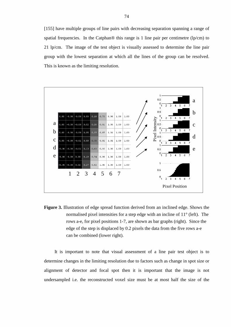
74

[155] have multiple groups of line pairs with decreasing separation spanning a range of

spatial frequencies. In the Catphan® this range is 1 line pair per centimetre (lp/cm) to

21 lp/cm. The image of the test object is visually assessed to determine the line pair

group with the lowest separation at which all the lines of the group can be resolved.

This is known as the limiting resolution.

a

bc

d

e

a

b

c

d

eP

ixel

Inte

nsi

ty

Pixel Position

4321 5 6 7

Figure 3. Illustration of edge spread function derived from an inclined edge. Shows the

normalised pixel intensities for a step edge with an incline of 11° (left). The

rows a-e, for pixel positions 1-7, are shown as bar graphs (right). Since the

edge of the step is displaced by 0.2 pixels the data from the five rows a-e

can be combined (lower right).

It is important to note that visual assessment of a line pair test object is to

determine changes in the limiting resolution due to factors such as change in spot size or

alignment of detector and focal spot then it is important that the image is not

undersampled i.e. the reconstructed voxel size must be at most half the size of the

75

limiting resolution spatial frequency. This is an important consideration for CBCT

where reconstruction times increase significantly with reducing voxel size.

A practical method to automate the analysis of images of a bar pattern or line pair

test object is to calculate the variance of the bar patterns with different frequencies

[156]. One advantage of this method is that it is more reslient to aliasing due to under-

sampling of the image (large voxel size) [157]. The method is used in the automated

analysis of portal images of the QC3V phantom with the PipsPro™ software (Standard

Imaging Inc., Middleton, Wisconsin, USA) [158]. Alternatively, the MTF can be

calculated more accurately directly from a line pair test object [159,160].

Chen et al. [161] demonstrated that the PSF can be calculated in three dimensions

from the edge spread function determined from the CBCT image of a plastic sphere.

The point spread function, which was modelled as a 3D-Gaussian distribution, was

determined iteratively by minimising the difference between the measured profile across

opposite edges of the sphere and a rectangular function convolved with the Gaussian

blurring point spread function. The full width at half maximum of the PSF is related to

the MTF50 which is the spatial frequency at which the MTF drops to 0.5. The method is

limited because only voxels along lines passing through the centre of the sphere were

sampled. This imposed the requirement that the reconstructed image voxel size was

small in order to sufficiently sample the edge profile. In their study the voxel size was

less than 0.2mm which is far less than the 1mm voxel size of the standard clinical

reconstruction setting on the Synergy® system. It should be noted that measurement of

the MTF from a large spherical object, as employed by Chen et al. makes the

assumption that the MTF is space invariant. This is not strictly correct as discussed and

demonstrated by Schwarzband and Kiryati [186] for spiral FBCT and CBCT systems.

In fact the MTF may also not be isotropic in the axial plane i.e. the same in all radial

directions. However, the method is likely to provide a reasonable consistency

measurement of image sharpness for the purpose of quality assurance.

76

In chapter 3, the concept of extracting the ESF from the image of a sphere is

utilised to extract the MTF50 from the ESF of the spherical air cavity at the centre of the

air-cavity within the QUASAR™ Penta-Guide phantom. A novel enhancement to this

method eliminates the dependence on small voxel sizes allowing the analysis to be

performed on a scan reconstructed with the standard resolution used clinically (voxel

size = 1mm x 1mm x 1mm).

2.5.2 Dual quaternions to represent rigid body transformations

In chapters 5-7 positional and image registration errors are represented as a rigid

body transform between the measured position and the 'ground truth'. Many researchers

express the errors as the difference in transform parameters but this is not strictly true

when there is a significant rotational component. The use of unit quaternions or versors

[102] provide a framework for dealing with the rotation component and can be used

during the optimisation process of image registration [102]. Dual quaternions provide a

convenient mathematical framework for representing both the translation and rotation

components rigid body transforms. They have been used extensively in the

aeronautical, computer graphics [162,163] and robotics [164,165] industries where

accurate interpolation and the computation of time varying position and rotation is

required to calculate trajectories.

Dual quaternions are particularly useful in simplifying the understanding of the

image registration error calculations. For instance the error between a registration result

and its ground truth can be defined as the unit dual quaternion that represents the

product of the unit dual quaternion conjugate representing the inverse of the measured

transform and the unit dual quaternion representing the ground truth transform. If this

were to be performed with the translation and rotation transforms separately, then the

order of the translations and rotations need to be considered carefully; with dual

quaternions this is all hidden within the framework of the dual quaternion. It also

provides a framework for calculating the average error transform. Methods for

77

calculating the average of a number of rotation transforms are discussed in the literature

[166-169]. However, it is not clear whether the translation parameters can be averaged

independently from the rotations; dual quaternions provide a solution to this problem

[163].

2.5.3 Evaluation of image registration similarity metrics

In chapter 8, the surface of the similarity metric is explored in the vicinity of the

transform parameters returned by an image registration. The choice of similarity metric

can influence the rate of success, speed and precision of an image registration.

Performing a near exhaustive search of the parameter space using several similarity

metrics is one way of predicting the likelihood of registration failure and precision. This

has been shown for megavoltage portal images in which the mean pixel-wise product

similarity metric was shown to have the least number of local minima with comparable

accuracy and reliability to the other similarity metrics tested [170]. Skerl et al. [171]

evaluated similarity metrics for CT-CBCT and CT-MR image registration. In their

study nine different similarity metrics were evaluated for image registration of two

vertebral bodies imaged with CBCT reconstructed using an iterative simultaneous

algebraic technique. They used five similarity metric evaluation metrics which relate to

accuracy, distinctiveness of the optimum, risk of non-convergence, number of minima

and capture range in order to demonstrate that the Asymmetric gradient– based mutual

(AMMI) similarity metric proved overall to give the best performance. They also

demonstrated that the AMMI metric gives reasonable results even when only four

projection images were used to reconstruct the CBCT image. Analysis of the similarity

metric over the parameter space has value in predicting the performance of a similarity

metric, independent of how the optimisation is implemented. But as demonstrated in

Chapter 8, may also be of value in evaluating the quality of an image registration.

78

2.5.4 Supervised Machine learning (Data mining)

In chapter 8, Bayesian networks are used to predict the quality of an image

registration based on a training set for which the misalignment between the two images

is known. In this section some of the basic concepts of machine learning relevant to the

work of Chapter 8 are introduced. Much of this is based on the book, 'Artificial

Intelligence, A modern approach', by Russell and Norvig [172]. Bayesian networks are

one of many supervised machine learning algorithms [172]. Supervised learning is the

term given to the problem of learning a function from examples of its inputs and

outputs. For example, linear regression is a simple form of supervised learning in which

a straight line function (y = m.x + c) is a hypothesis for the true function that gave rise

to the observed data. The parameters of the straight line i.e. the gradient (m) and

intercept (c) are learnt from a set of observations. These take the form of point data

with a single output (y) for each input (x). The parameters of the straight line can be

determined by minimising the squared difference between the outputs and the straight

line. The straight line is then used to predict the output on the basis of further inputs.

A common problem in the training of a machine learning algorithm is noise and

over-fitting. If a machine learning algorithm has too much freedom in the generation of

possible hypothesis then the model may predict the training data well but will

incorrectly predict the output based on further inputs. An example of this is fitting a

polynomial of degree n to n points (e.g. n = 6) where the n points are based on noisy

observations and the underlying function is actually a straight line. The model which

will have a series of maxima and minima will exactly fit the n observations but will not

be generalisable i.e. it will be unable to correctly predict the output for any other

observations which interpolate or extrapolate the training set. A general rule is that the

hypothesis should be the simplest that is consistent with the data (Ockham's razor). One

method of preventing over-fitting is cross-validation. The set of observations is split

into two groups, a training set and a test set. The hypothesis is learnt from the training

set and then used to predict how well it predicts the test set. In K-fold cross-validation

79

the data, consisting of N observations, is split into (k-1).(N/k) observations for the

training set and N/k observations for the test set. k experiments are run using a different

set of N/k observations as the test group each time.

Regression methods are used where both the inputs and outputs are continuously

variable. If the output is discrete i.e. one of a number of classifications then regression

techniques can still be employed by enforcing thresholds to the output. There are a

number of other algorithms that can be utilised. The simplest are based on discriminant

functions which divide the input variable space into regions containing the different

classes. However,

"statistical learning algorithms can provide general solutions to

the problems of noise, over-fitting and optimal prediction."

[172]. The simplest of these is the Naive Bayes model which assumes that all the

independent variables are independent. The output has a conditional probability on each

of the input variables which is learnt from the training data set. Given a new set of

inputs the output prediction of classification is the product of the probability of

observing the class and the geometric sum of all the conditional probabilities of the

inputs. The Naive Bayes model scales well to large problems and has no difficulty with

noisy data however, it is likely to fail if the input variables are not independent. The

Bayesian Network algorithm [173] can be used where the input variables are not

independent. The Bayesian Network creates a network of interdependent variables in

which the conditional probabilities of one input variable on another are determined. In

the extreme case all input variables are dependent on each other. Typically not all

inputs have conditional dependence on all other inputs and so the network maybe much

simpler. A Bayesian network is learnt in two stages [174]. First the network is learnt

using optimisation methods, often using the Naïve Bayes model as a starting point and

then the conditional probabilities are learnt. Other statistical machine learning

algorithms that are commonly used, which could have been applied to the problem

addressed in chapter 8, include Neural Networks and Support Vector machines [172].

80

Machine learning has been used in radiotherapy applications by a number of

researchers in predicting radiotherapy outcome [175-179] and also in image guided

radiotherapy for markerless respiratory gating of radiotherapy treatments [180].

However such techniques have not been applied to the problem of learning image

registration quality.

2.6 Summary

In this chapter image guided radiotherapy has been introduced and the published

literature relating to geometric uncertainties considered. Geometric uncertainties can be

divided into three distinct areas of image geometry, image registration and correction.

A need for accurate and efficient methods for quality assurance of the alignment of both

the CBCT image and the treatment beams has been identified. There is very little

information on the performance of automatic image registration algorithms used for

CBCT based image guidance and the lack of access to the algorithms restricts the

thoroughness to which they can be tested. Furthermore, there is no standardised method

of reporting image registration accuracy. It is the aim of this thesis to develop

techniques to measure image registration performance and to further our understanding

of the accuracy, precision and robustness of the image registration algorithms used in

IGRT. In particular their ability to work with high noise, low dose images is of interest

in order to reduce the risks that are associated with X-ray imaging. Finally, the thesis

aims to perform a preliminary exploration of a method to provide user feedback on the

likely quality of an image registration.

Chapter 3

Quantification of misalignments in cone beam

CT based IGRT equipment

3.1 Introduction

By integrating a CBCT imaging system with a linear accelerator (linac) i.e.

mounting the X-ray tube and amorphous silicon flat panel imager to arms that project

from the linac gantry, the CBCT image should be inherently aligned with the MV

treatment beam. However, to ensure correct alignment between MV and CBCT

systems, the CBCT system needs to be calibrated. This will eliminate the small

systematic misalignments of tube and imager and the effects of mechanical sag due to

gravity. If, for some reason e.g. the actions of servicing or component failure, the

calibration becomes invalid then a misalignment between MV and CBCT systems could

be introduced. This would lead to errors in image guidance i.e. the misalignments will

lead to geographic miss of the target affecting the quality of the treatment. It is therefore

essential that an appropriate schedule of checks is made to ensure significant

misalignments are detected before they affect patients' treatments. It is also important to

determine the typical day to day variation of these misalignments. If this variation is

significant then it needs to be factored into treatment margin calculations [21].

Misalignments of X-ray tube and imager may also cause loss of image sharpness which

will affect the ability to perform image registration. As with the CBCT-MV alignment

82

these effects need to be measured regularly to determine their effect on the image

guidance process.

In this chapter methods of quantifying CBCT to MV isocentre alignment and X-

ray tube to imager alignment are described and historical results reported. A new

method to improve the measurement of CBCT to MV isocentre alignment is described

in detail and tested. A novel method of measuring the image sharpness performed on

images acquired during the CBCT to MV isocentre alignment measurement is also

described Its sensitivity to misalignment of the imager is demonstrated and compared to

results obtained using the Catphan® 600 image quality phantom The literature suggests

that CBCT-MV alignment errors are low. However, to ensure these complex systems

remain aligned, methods for performing routine checks, in an efficient manner, need to

be developed. This can only be achieved if all checks of the linac and image guidance

systems that need to be performed frequently (daily or weekly) are combined so that

they all use the same phantom. It is important that the reduction in time taken to

perform these checks does not compromise levels of accuracy and precision.

3.2 Background

In 2005 Leeds Teaching Hospitals NHS Trust took delivery of the first commercial

Synergy® system to be installed in the UK. A quality assurance scheme was established

which concentrated primarily on the geometric aspects of the system. A CBCT-MV

isocentre alignment test was established using the Elekta ball bearing phantom as used

by Lehmann et al [60]. The ball bearing (BB) was aligned to the room lasers (nominally

the MV isocentre) and its position relative to the MV radiation isocentre determined

using the MV portal imager. In contrast to Lehmann et al, the ball bearing was not

adjusted to match the MV radiation isocentre and the BB was imaged using a

reconstructed CBCT image instead of just two orthogonal kV projection images. Note,

for the measurement of CBCT-MV isocentre it is not necessary to have the BB placed at

the MV radiation isocentre. It just needs to provide a common point of reference for

83

both kV and MV imaging systems that is close to the MV isocentre. Registration of the

CBCT image with a reference image gave the shift between BB and CBCT image

centre. The difference between BB position relative to both the MV isocentre and the

CBCT image centre gave a measure of the CBCT-MV isocentre alignment. The BB

was imaged with the three fields of view and the whole procedure took approximately

45 minutes. While this gave a very accurate assessment of CBCT-MV alignment it was

not practical as a daily check and even on a monthly basis the measurement could not be

fitted into the time allotted for performing routine checks of the linac.

Since the most likely cause of a misalignment between MV and CBCT system was

the panel not being driven to the correct position for imaging, a very quick daily check

was introduced. This check used a special filter inserted in the collimator assembly of

the X-ray tube with a radio-opaque cross at its centre. A 2D projection image acquired

daily was compared to an equivalent image acquired immediately after flexmap

calibration of the system at a gantry angle of 0°. Flexmap calibration, described in 2.2.4

is used to set-up the position of the MV isocentre in the CBCT image. The location of

the cross on the daily image was compared to the reference image. At this time the

Synergy® system had no in-built safety mechanism to ensure the panel was in the

correct place for imaging. If an image was acquired with the imager misaligned in the

longitudinal direction i.e. parallel to the rotation axis then the CBCT image would look

normal but image registration against a reference image would give erroneous patient

correction shifts. Misalignment of the imager in the lateral (tangential) direction would

not lead to the wrong patient shifts but would reduce the sharpness of the image as

discussed previously. While the quick panel alignment check could not ensure that the

panel always drove to the correct place for each image it could at least check the

position at the beginning of the day and could be monitored to assess the random error

and any systematic drifts. An added advantage of the panel alignment check was that it

could detect lateral misalignments of the panel which would not necessarily be picked

up by the CBCT-MV isocentre check

84

In the period 2008-2010 Leeds led a national project to evaluate X-ray

tomographic IGRT systems for the Centre for Evidence based Purchasing (CEP). As

part of this evaluation there was a need to develop a method to assess the CBCT-MV

isocentre alignment using methods that were independent from any single manufacturer

and could be applied to any manufacturers CBCT system. At this time the QUASAR™

Penta-Guide phantom had recently become commercially available. The Penta-Guide

phantom (Figure 4) combines kV-MV alignment tests with positioning accuracy. As

described by Bisonnette et al [9];

The Penta-Guide phantom "consists of 5 low-density spheres set in

a unique spatial orientation and embedded within a 16-cm block of

acrylic. The central sphere has a diameter of 12 mm, whereas all of the

others have a diameter of 8 mm. Each sphere, except the central 12-mm

sphere, has a matching low-density ring on the posterior and right-hand

faces, such that anterior and lateral-left projections of the spheres

should be concentric with the rings if the cube is levelled. The 5 spheres

are oriented in a unique pattern to distinguish right from left, anterior

from posterior, and superior from inferior orientations. All materials

were chosen to minimize CT artifacts" ..." The unique spatial distribution

of the sphere allows the verification of the geometric accuracy and

integrity of planar images obtained in either radiographic or

fluoroscopic modes. Displacement of the central sphere from the center

of the image matrix will indicate misalignment of the x-ray tube and/of

flat-panel assemblies with respect to the accelerator isocenter;

noncoincidence of the sphere and matching ring will indicate rotation of

system components (tilt, pitch, or yaw); and finally, mismatches between

the expected and actual orientation of the sphere will indicate issues with

85

the image-acquisition system or acquisition software. Finally, the marks

and etchings engraved on the phantom’s surface integrate the daily QA

of volumetric image guidance systems with actual accelerator daily

QA."... "the surfaces of the phantom were engraved with markings to

align the phantom with the room lasers and subsequently assess the size

of the light field, the position of the cross-hairs, and the optical distance

indicator on 3 of the 4 cardinal gantry angles (ie, 0°, 90°, and 270°).44

Therefore, daily QA of the image-guidance system can be performed

simultaneously with several daily QA procedures, minimizing the

additional time required to perform daily QA for all of these components

while improving their accuracy."

(a)

(b)

Figure 4. The Penta-Guide phantom. a) Photograph of Penta-Guide phantom and b)

translucent illustration of phantom showing internal air cavities. (Images

courtesy of Modus Medical Devices Inc. London, ON, Canada).

86

The use of 2D-2D matching of DRRs and MV portal images from just two gantry

angles was thought to be a less accurate technique than the ball bearing CBCT-MV

isocentre alignment test. It also introduced a greater degree of subjectivity as the 2D-2D

match required manual location of the field edges and manual location of the central

sphere with the iView portal imaging software (Elekta AB, Stockholm, Sweden).

It was also recognised that the current daily panel alignment test did not test the

full functionality of the Synergy® system prior to clinical use and in particular that no

check of the couch positioning accuracy was being made. The Penta-Guide phantom

was ideal for this; however as an additional check it was likely to extend the length of

daily QA by some 20 minutes or more. The Penta-Guide phantom also had appropriate

markings for checking the room lasers, optical field and distance indicators. These tests

were currently checked using an alternative test tool. The Penta-Guide had the potential

to reduce the overall time to perform daily QA, if, both the standard linac QA, the check

of CBCT-MV isocentre alignment and couch positioning could be integrated.

Furthermore it should be possible to measure the sharpness of the edge of the

central spherical air cavity in the CBCT image. This would avoid an additional CBCT

scan of the Catphan® to assess image sharpness as it could be performed on the same

scan of the Penta-Guide phantom as was used for CBCT-MV isocentre alignment. The

image sharpness test has the potential to detect the lateral misalignment between X-ray

tube and imager.

3.3 Methods

3.3.1 CBCT-MV isocentre alignment using the ball bearing phantom

The CBCT-MV isocentre alignment was measured once a month, using an 8mm

ball bearing (BB) phantom provided by Elekta with the Synergy® system for calibrating

the flex in the system. The alignment was determined in two stages: first, the position

87

of the BB relative to the MV isocentre was measured using the iViewGT portal imager;

second, the position of the BB in a CBCT scan, was measured, relative to a digitally

synthesized reference image of the BB with a treatment centre placed at its centre. The

CBCT-MV alignment was given by the vector difference between these two

measurements.

The MV isocentre was measured using an image analysis software tool provided

by Elekta in the X-ray Volumetric Imaging (XVI) (v3.4) software application of the

Synergy® system. First, two portal images were acquired at each of the four cardinal

gantry angles (0°, 90°, 180° & 270°) with the BB aligned to the lasers (nominal MV

isocentre). Each pair of images was acquired with a square field (12cm x 12cm) and

opposing diaphragm rotations (90° & 270°). For efficiency this was performed using a

step and shoot intensity modulated radiotherapy beam to cycle through each of the

beams while the imager automatically acquired images for each segment. The XVI

software analysis tool was then used to locate the projected centre of the radiation field

on each image from the edges of the diaphragm and the centre of the BB on each image.

Locating the field centre on images acquired with opposing head angles accounted for

any miss-calibration of the field edge position. The analysis tool calculated the 3D

coordinates of both the MV isocentre and BB positions by back-projecting the

respective image coordinates from all four gantry angles to the isocentric plane, a

distance of 100 cm from the source. For the purpose of flexmap acquisition, the

intended use of the XVI software tool, the relative difference in position of BB would

have been used to reposition the BB at the MV isocentre however, for the purpose of

measuring CBCT-MV isocentre alignment this was not necessary.

The second stage of measuring CBCT-MV isocentre alignment was to acquire a

CBCT of the BB reconstructed at (0.5 mm)3 voxel size. Image registration with a

synthesized image of the BB allowed the displacement of the BB from the reference

image to be determined using the registration tools available in the XVI software

application. CBCT-MV isocentre alignment was calculated from the difference between

88

the vectors describing both BB centre to MV isocentre displacement and displacement

of BB in the CBCT scan.

This method was performed monthly over a period of almost two years for each of

the small, medium and large fields of view (Figure 5. a-d) available with Synergy® as

part of a routine quality assurance program for IGRT. A separate flexmap calibration

was required for each field of view because each field of view had its own nominal

position of the flat panel imager. Consequently, each field of view was checked on a

monthly basis.

41

100

53.5

26.7

≈ 40 ≈ 50

(a) (b)

(c) (d)

Figure 5. Diagram of Elekta Synergy® system and its geometry for each field of view. (a)

Schematic of the Elekta Synergy® system showing kV imager (U, V) and

isocentre (X, Y, Z) coordinate systems, (b) illustration of small field of view

geometry, (c) illustration of medium field geometry and, (d) illustration of

large field of view geometry. (All dimensions are in units of cm.)

89

3.3.2 Daily check of flat panel imager alignment

A daily check of flat panel imager alignment was implemented as part of a quality

assurance scheme to indicate any change in the mechanical set-up of the Synergy®

system that might lead to either CBCT-MV centre misalignment or image blurring. The

method was based on that first implemented at the Christie Hospital (Manchester, UK)

but not described elsewhere in the literature [181]. This check required the acquisition

of a 'Planar View’ kV image acquired with a static gantry angle of 0° with a custom

filter inserted into the filter slot of the X-ray tube housing. The custom filter, known as

'CAL1' and supplied with the Synergy® system, had a cross that projects approximately

to the isocentre. For the daily imager alignment check the position of the cross was

compared to that in a reference image, acquired in a similar manner, at the time of

flexmap acquisition, using the template matching tools in the XVI software. A

difference in the position of the cross in the check image relative to the cross in the

reference image indicated a misalignment of the source and imager.

Alignment check images performed both at small and medium fields of view, over

a 7 month period, were reviewed to determine the stability of the system and hence

assess the value of the check. To do this images were exported in DICOM format and

then analysed using locally developed Matlab code (The MathWorks, Inc.) to

automatically locate the position of the cross on each image and compare it to the

position of the cross in the reference image.

3.3.3 Measurement of CBCT-MV isocentre alignment using the Penta-

Guide phantom

The Penta-Guide phantom used, was a 16cm cube of Acrylic, with five, internal,

spherical air cavities with unique orientation for 3D image registration and external

markings for checking laser alignment, MV light field size and anterior-posterior and

lateral kV projection alignment. The CBCT-MV isocentre alignment was measured

with the Penta-Guide phantom in a similar manner to that using the BB phantom

90

(section 3.3.1) but with the central air cavity of the Penta-Guide phantom replacing the

BB. The central air-cavity of the Penta-Guide phantom, which was 12mm in diameter,

was slightly larger than the diameter of the BB, 8mm. The Penta-Guide phantom was

aligned with the lasers and eight portal images acquired using the same method as for

the BB phantom. The eight images were then exported in DICOM format for analysis

by locally developed software written using the Matlab programming language. This

tool performed the same function as the Elekta tool except portal images of the Penta-

Guide phantom were used instead of the BB phantom. Details of the analysis performed

by this software tool follow.

3.3.3.1 MV radiation field centre localisation

First the radiation field centre was located for each of the eight portal images by

calculating the geometric centre of the 12cm square radiation field which is defined by

its radiation field edges (Figure 6). To locate the field edges, first a Canny edge

detection [182] was used to extract all edges in the image (bottom right hand corner of

Figure 6). The Canny edge detection located noise in the image as well as the field

edges. To locate pixels corresponding to the field edge a binary mask was applied

which contained all values between an upper and lower intensity threshold. These limits

were chosen by first finding the two peaks in the image histogram corresponding to

pixels that were either inside or outside the radiation field. Only voxels with intensities

between 25% and 75% of the voxel intensity range between the two peaks were selected

(Figure 7). The 25% and 75% lower and upper limits were determined empirically.

The binary mask was used to select only the edge pixels, located using the Canny edge

filter, that related to the radiation field edge (grey region adjacent to Canny edge

detection pixels in bottom right hand corner of Figure 6).

91

Figure 6. MV portal image of the Penta-Guide phantom zoomed in on the radiation

field. Regions encompassing each of the air-cavities have been augmented

by rescaling the image data. The lower right corner of the image has been

replaced with a combination of the edge data extracted using the Canny edge

filter (white) and the field edge mask (grey). The positions of the field

edges determined by the Hough transform (dashed lines), field corners ('□')

and field centre ('*') are also shown as well as the centre of the air cavity

('o').

To determine the equations of the four straight lines corresponding to each field

edge, first a linear Hough transform [183,184] was applied to the image of radiation

field edge pixels. The Hough image was produced by transforming the pixel

coordinates (x,y) of all edge pixels in the real space image into a straight line defined by

Equation 3 (Figure 8). The Hough image is a discretisation of (ρ,θ) space. In this case

the interval between pixels along ρ was 0.25mm, the size of each pixel in the real space

92

image and the interval between θ was 0.25°. A count was added to all pixels in the

Hough image which intersect the straight line and this was repeated for all edge pixels in

the real space image.

θθρ sin.ycos.x += Equation 3

Since the edge pixels along the four field edges form a near straight line, the

Hough image contains four strong peaks. The four peaks are located by first finding the

brightest pixel, which is the location of the first peak. A region around the first peak is

set to zero and the next highest peak located. This is repeated until all four peaks have

been located.

2 2.5 3 3.5 4 4.5 5 5.5 6 6.5

x 105

0

0.2

0.4

0.6

0.8

Pixel intensity

Fre

quen

cy (

%)

Figure 7. Frequency distribution of the pixel intensity values in the MV portal

image.The lower and upper peaks correspond to pixels within the radiation

field and outside the radiation field respectively. The grey shaded area

indicates the lower and upper thresholds used to create a mask of pixels

adjacent to the field edge.

The intersection of each pair of lines is then calculated by first sorting the four

values of ρ and θ so that they correspond to adjacent lines i.e. upper, right, lower and

left. The x and y coordinates of the corners (Figure 6) are then calculated using

93

Equation 4 where i and j are used in the order given. The x and y location of the

radiation field centre is calculated by averaging the four xi and yi corner coordinates.

( )( )

( )( )

==

⋅−⋅⋅−−

=

⋅−⋅⋅−

=

1,4,3,2j

4,3,2,1i

sincossincos

coscos.y

sincossincos

sinsin.x

ijji

ijjii

ijji

ijjii

θθθθθρθρ

θθθθθρθρ

Equation 4

The intersection of the beam axis on the MV flat panel imager for each gantry

angle was calculated by averaging the radiation field centres located on the

corresponding pair of images with opposing head angles (Figure 5. ).

θρ

x

y

Figure 8. Illustration of the linear Hough transform. Shows the angle θ, between the

straight line and the x-axis and the distance ρ, which is the shortest distance

between the straight line and the origin.

94

3.3.3.2 Penta-Guide air cavity centre localisation using MV images

The projected centre of the air cavity on each image was determined by: 1)

extracting a 64 x64 pixel sub-region centred on the image centre that contained just the

air cavity and a small amount of the surrounding phantom, 2) applying a low pass

convolution averaging filter with kernel, dimensions of 10 x 10 pixels, to blur the image

and reduce high frequency noise, 3) extracting the maximum gradient using

morphological operators, 4) applying a threshold to the maximum gradient image using

an empirically derived level to segment only the edges relating to the air cavity and not

the projection of the rings on the phantom surface and 5) locating the centre of the circle

that best fits the resulting image. This last step was performed using an unconstrained

multivariate derivative free simplex search routine [185] to maximise the sum of all

pixel values in the thresholded maximum gradient image that are located under the

circle. Figure 9 shows both the original (a) and maximum gradient images (b) with the

located circle superimposed.

The projected centre of the air cavity was calculated for all eight images. For each

gantry angle the air cavity centres located on the two images with opposing head angles

were averaged.

3.3.3.3 Back projection

A nominal origin was constructed assuming the centre of the imager back-

projected to the isocentric plane for all gantry angles to a single point. The intersections

of the beam axes, relative to the centre of the image, for all gantry angles, were back-

projected to the isocentric plane and the average of these coordinates defined the MV

isocentre in 3D. Similarly the centres of the air cavities were back-projected to define

the 3D coordinate of the centre of the air-cavity in the Penta-Guide phantom. The MV

isocentre to air-cavity centre distance was given by the difference between these two 3D

coordinates. For the purpose of comparing the localisation of the MV isocentre with the

95

Elekta software both the MV isocentre location and the MV isocentre to air-cavity

centre distance were reported separately.

Figure 9. MV portal image of air-cavity in Penta-Guide phantom. a) zoomed in section

of a MV portal image of air-cavity in Penta-Guide phantom and b)

corresponding unthresholded maximum gradient image. Both images show

the position of the circle template and its centre found from gradient based

optimisation.

3.3.3.4 XVI centre to air-cavity centre alignment using the Penta-Guide phantom

To determine the relative position of the CBCT image centre and the air-cavity the

Penta-Guide phantom was first scanned using a Siemens Sensation 40 Open CT scanner

(Siemens Medical Solutions, Erlangen, Germany) with 0.6mm slice thickness and

0.5mm in-plane pixel size. This was sent to the Xio treatment planning system (Elekta

AB, Stockholm, Sweden) where the air cavity was contoured using a simple threshold

technique. An isocentre was placed at the geometric centre of the air-cavity structure

using an option within Xio and a single beam set to the isocentre for the purpose of

sending to Synergy®. A CBCT scan was performed with the Penta-Guide phantom in

the same position as in section 3.3.3, and reconstructed with a voxel size of (0.5mm)3

96

before it was manually registered with the CT scan, using the XVI application tools.

This gave the relative shift between CBCT image centre and air-cavity centre.

Finally, the CBCT-MV alignment was calculated by taking the vector difference

between air-cavity centre to MV isocentre displacement and air cavity displacement

measured using the XVI scan.

3.3.3.5 Repeatability, reproducibility and comparative tests

To determine repeatability of the CBCT-MV isocentre alignment calculation five

repeat sets of eight MV images were acquired without moving the phantom. The

Matlab analysis software described in section 3.3.3 was used to determine the MV

isocentre to air-cavity alignment for each set.

To compare both methods a reproducibility study was performed using both the

BB with XVI analysis tool and the Penta-Guide phantom with our locally developed

analysis tool.

For reproducibility the CBCT-MV alignment measurement was repeated eight

times for both the BB phantom and Penta-Guide phantom techniques. The

measurements were performed alternately so that the BB and Penta-Guide phantoms had

to be re-positioned for each measurement. This reduced the possibility of a systematic

difference between the two sets of measurements. The mean and standard deviation of

the CBCT-MV alignment was calculated for both techniques and compared.

3.3.4 Method for approximating the image sharpness from CBCT scans of

the Penta-Guide phantom

Misalignments of the flat panel imager with the X-ray source have different effects

depending on whether they are parallel or perpendicular to the axis of rotation. A lateral

displacement parallel to the axis of rotation (V) will affect the CBCT-MV alignment

and have minimal effect on the image sharpness while a displacement perpendicular to

97

the axis of rotation (U) will reduce the image sharpness while having minimal affect on

CBCT-MV alignment (Figure 5. ).

The image sharpness was measured by calculating the MTF [152] based on the

edge response function of profiles extracted from the scan data across the interface

between air and phantom of the central air cavity in the Penta-Guide phantom. This is

similar to the method used by Chen et al. [161]. The scan data was exported in DICOM

format for analysis. The profiles of CBCT image data were constructed from voxels

within cones radiating from the centre of the air cavity. The image voxel values within

a single cone were collapsed into a single profile according to each voxels radial

distance. A least squares fit to the profile data of an edge response function (ESF)

modelled on a Gaussian point spread function (PSF) was performed to determine the

width of the PSF. By sampling conical sections of data the sampling frequency across

the edge of the air cavity was increased. This enabled the pre-sampled MTF to be

estimated even when the images were reconstructed with a (1mm)3 voxel size, the

setting used in clinical practice. The analysis was implemented using Matlab, details of

which are described in the following text.

3.3.4.1 Locating the centre of air cavity

The image data from a 3D sub-region of the scan centred on the air cavity, was

extracted, inverted and scaled to the range [0 to 255]. The centre position was

calculated by taking the weighted average of the coordinates of the centre of all voxels

with values greater than 20% (51). The average was weighted using the scaled voxel

intensity. Let M be the sub-region containing the spherical air cavity with all pixels

having a value greater than 51. Let i, be an index to one of the voxels in the sub-region,

M, with coordinates xi, yi and zi and voxel intensity I i. The coordinates of the air cavity

centre (Cx,Cy, Cz) is given by, Equation 5.

98

∑

∑

∑

∑

∑

∑

∈

∈

∈

∈

∈

∈

⋅=

⋅=

⋅=

Mii

Miii

z

Mii

Miii

y

Mii

Miii

x

I

zI

C

I

yI

C

I

xI

C

Equation 5

The 20% threshold value was sufficient to remove the influence of a faint,

propeller shaped, reconstruction artefact that exists, adjacent to and outside the sphere

cavity. These are visible in the axial view (Figure 10). The 20% threshold was

determined empirically.

3.3.4.2 Extracting profiles

Conical regions of image data about radial lines, centred on the air cavity, were

collapsed into radial profiles (Figure 11). First, the Cartesian coordinates (x, y, z) of the

centre of every voxel relative to the air-cavity centre was calculated and then converted

into spherical coordinates (r, θ, ϕ). Image data within a conical section and oriented

along selected radial directions were ordered in ascending values of radial distance (r).

Radial profiles were selected at equal radial angle intervals in the axial plane e.g.

[-15π/16, -14π /16, ..., 15π/16, π]. The opening angle of the cone was set to the same as

the radial angle interval e.g π/16. Two profiles, sampled from cones pointing in opposite

directions along the rotation axis were also extracted.

99

Figure 10. Effect of CBCT panel alignment on sharpness of Penta-Guide phantom air

cavity. Transverse (a,d), sagittal (b,e) and coronal (c,f) cuts through a CBCT

scan of the Penta-Guide phantom, zoomed into a region about the central air

cavity, after first inverting and normalising the grey scale. The first row

(a,b,c) shows the sharpest image reconstructed with a simulated imager

displacement of -0.2mm in the U direction (fifth scan) while the second row

(d,e,f) shows the same scan reconstructed with an imager displacement of

+1mm.

100

x

yz

r

r

Figure 11. Illustration of the spherical air-cavity and four conical sections. Conical

sections are centred on the x and y axis of the trans-axial plane through the

centre of the sphere. Each voxel within the cone such as the one shown is

collapsed onto the conical axis with radius r to create an edge response

profile.

3.3.4.3 Fitting the edge response function

A Gaussian model was assumed to approximate the point spread function. The

Gaussian blurring of a rectangular edge gives the error function (Equation 6). This was

used as a model (Equation 7) for a least squares fit of the profile data using the simplex

search method [185].

( )∫ ⋅−=r

dttrerf0

2exp2

)(π

Equation 6

101

( )[ ]( ){ }321 1 xrxerfxxr ofit −⋅−⋅+= Equation 7

where x0, x1, x2 and x3 were the parameters of the fit, r was the radial distance

from the origin along the collapsed cone axis and rfit was the modelled data.

Using the theory described by Boone and Seibert [153], but not including the

additional exponential term for scatter the MTF was described by Equation 8 from

which the MTF50 was calculated Equation 9.

222 / xfeMTF π−= Equation 8

where f is the frequency.

( ) π/)2ln( 21

250 xMTF ⋅= Equation 9

MTF50 was defined as the frequency, at which the MTF was reduced from 1 to 0.5.

Figure 12. shows an example of a collapsed cone radial profile with the error

function fit and corresponding MTF curve.

102

Figure 12. (a) Example of a radial profile along a collapsed cone with the error function

fit and (b) corresponding MTF curve.

3.3.4.4 Repeatability of MTF50 calculation and sensitivity of MTF50 to panel

misalignment

The Penta-Guide phantom was scanned once on the Synergy® system and then a

few weeks later, a further four repeat scans were taken. Both imager and panel were

retracted and re-deployed between scans. Each scan was reconstructed twice with

isotropic voxel sizes of (0.5mm)3 and (1mm)3 respectively. The MTF50 was calculated

for both axial and longitudinal directions using the method described in sections 2.4.1

and 2.4.2 and with equal cone angle and radial profile angle intervals of π/4,

π/8 and π/16.

103

The sensitivity of the measurement of MTF50 to potential misalignments of the

panel was investigated by simulation. Each of the five CBCT scans of the Penta-Guide

phantom were repeatedly reconstructed after adding a constant offset to the flex data in

the U direction. This was achieved by directly re-writing the flexmap data in the system

database. The offsets added to the flexmap ranged from -1mm to 1mm in 0.2mm

intervals. This process was repeated for all five CBCT scans of the Penta-Guide

phantom. Figure 10d-f shows transverse, sagittal and coronal cuts through a

reconstruction of the Penta-Guide air cavity with a shift of 1mm. For one scan only

constant offsets between -1mm and 1mm in 0.2mm intervals were also added in the V

direction. For each reconstruction the MTF50 was calculated for radial profiles in both

the transverse (X-Z) plane and along the rotation axis (Y).

To compare the MTF50 measurements on the Penta-Guide phantom with the

limiting resolution measured using the Catphan® 600, the Catphan® was also scanned

and reconstructed with both (0.5mm)3 and (1mm)3 voxel sizes with simulated panel

shifts between -1mm and 1mm in 0.2mm intervals. The line pair resolution test pattern

in the CTP528 section of the phantom was viewed and assessed to determine the

limiting resolution for each reconstruction.

3.4 Results

3.4.1 CBCT-MV isocentre measurements using the Ball Bearing phantom

The CBCT-MV isocentre alignment was found to be stable over the two year

period during which these measurements were performed (Table 1). The absolute

values of the MV isocentre were not reported as they were referenced to an arbitrary

point in space and were therefore meaningless. However the standard deviation was

considered to be a measure of both the MV system stability and the measurement

method reproducibility combined. The elevated standard deviation in the longitudinal

direction was due to two consecutive measurements where the MV imager appeared to

104

have been shifted approximately 1mm in the longitudinal direction. This did not affect

the measurement of the positional difference between MV isocentre and BB position or

the measurement of CBCT to MV isocentre alignment as both would have been shifted

by equal amounts.

Assuming the position of the MV isocentre was static during the period of

measurement and that the BB was aligned with the lasers during these measurements,

the positional difference between MV isocentre and BB position indicated a

combination of the accuracy to which the lasers were aligned with the radiation

isocentre and the reproducibility of aligning the phantom to the lasers. The standard

deviation of this measurement was better then 0.5mm in all directions. It should be

noted that the lasers were aligned to the mechanical isocentre at least twice during the

measurement period and not to the radiation isocentre hence the small systematic

difference ( < 0.5mm) between laser position and MV isocentre was expected. The

increased variability of this measurement may have been due to the precision with

which the BB could be aligned to the lasers.

The mean position of the CBCT to MV isocentre alignment was less than 0.12 mm

in all directions for all fields of view. The maximum standard deviation observed was

0.27mm which occurred in the Y direction. The maximum absolute deviation of the

CBCT to MV isocentre was found to be 0.54mm in the longitudinal direction.

105

Table 1. MV isocentre position, difference between MV isocentre and BB position and difference between CBCT image centre and MV isocentre in each of the lateral (X), longitudinal (Y) and vertical (Z) directions. CBCT-MV alignment is reported for the small, medium and large field of views (SFOV, MFOV and LFOV). All results are reported as mean and (one standard deviation).

Lateral Longitudinal Vertical

X (mm) Y (mm) Z (mm)

MV iso (N=22) - (0.11) - (0.29) - (0.17)

MVIso – BB (N=22) 0.30 (0.37) 0.34 (0.29) 0.48 (0.43)

SFOV: CBCT-MV iso (N=22) 0.09 (0.10) -0.06 (0.23) -0.05 (0.15)

MFOV: CBCT-MV iso (N=22) 0.12 (0.11) -0.01 (0.27) -0.02 (0.18)

LFOV: CBCT-MV iso (N=20) 0.04 (0.16) -0.01 (0.27) -0.07 (0.24)

3.4.2 Daily check of panel position

Over a seven month period there were a total of 73 small field of view and 74

medium field of view daily alignment checks. The large field of view was not checked

because it was not used routinely during this period. All measurements of misalignment

were scaled back to the isocentric plane (Figure 13). The mean [U,V] misalignments

were [-0.4mm, -0.5mm] and [-0.5mm,-0.4mm] for the small and medium fields of view

respectively. There was a similar spread of results in both directions and for both fields

of view. The standard deviations for all four combinations were between 0.3mm and

0.4mm and maximum deviations were as large as 1.5mm. For the small field of view

there was a time trend towards increased panel offset in the U direction and decreased

offset in the V direction over the period of observation. Regression analysis showed

that the slope was significant (P < 0.0001) for U but not for V. A similar trend was

observed for the medium field of view but this time the slope was not significant for U

and was significant for V (P < 0.0001). Interestingly the initial offset in the small and

106

medium field of view was ≈ 0.5mm in the U. The implications of this are discussed

later.

Figure 13. Results of daily alignment checks. Plots show measured offsets in the U and

V directions using the custom filter (Section 3.3.2) for small and medium

fields of view (SFOV, MFOV) plotted as a function of time. The solid line

represents a linear least squares fit to the data. The slope is significant for

(a) and (d) but not for (b) and (c).

3.4.3 CBCT-MV isocentre alignment repeatability and comparative tests

The five sets of measurements in which the Penta-Guide phantom was imaged

without re-positioning showed the MV isocentre and air-cavity centre localisation to be

highly repeatable. The standard deviation of the residual errors combined for the X, Y

107

and Z directions was 0.05 mm for the MV isocentre location and 0.04mm for both the

air-cavity and the difference between MV isocentre and air-cavity centre.

Both the Penta-Guide and BB methods of measuring CBCT-MV isocentre

alignment were highly reproducible with little difference between the two methods

(Table 2). For localisation of the MV isocentre there was little difference in the mean

co-ordinates using the two methods. There was also no significant difference between

the standard deviation of the residual errors. For the CBCT-MV alignment the largest

difference between the two methods was 0.15mm, in the X direction, while the smallest

was 0.02mm, in the Y (vertical) direction. All differences were less than the size of one

pixel (0.25 mm at the isocentric plane). The standard deviation using the Penta-Guide

phantom (0.15mm) was significantly larger than that observed with the Ball bearing

(0.09mm) (F-test, P < 0.05).

Table 2. Mean and standard deviation of residuals for MV isocentre and CBCT-MV alignment using both the ball bearing and Penta-Guide methods.

Mean

X (mm) Y (mm) Z (mm)

σσσσ(residual) (mm)

Ball Bearing -0.23 -2.35 -0.07 0.03

Penta-Guide -0.23 -2.31 -0.07 0.04 MV isocentre

Difference 0.01 0.04 0.01 -

Ball Bearing 0.26 0.06 -0.02 0.09

Penta-Guide 0.41 0.08 0.06 0.15 CBCT-MV alignment

Difference 0.15 0.02 0.09 -

108

3.4.4 MTF 50 calculation from Penta-Guide Phantom

There was a noticeable variation in MTF50 with the radial direction of the

collapsed cone profile in the axial plane. Figure 14 shows the MTF50 measured three

times on the first CBCT scan with cone angle and cone spacing of π/4, π/8 and π/16

radians respectively. The ability to resolve variations with radial angle was increased as

the cone angle and spacing was reduced. The variation in MTF50 was clearly periodic

with the radial direction of the sampling. This was attributed to low frequency shading

artefacts observable in the axial plane (Figure 10a). The peaks in the measured MTF50

(~0.3 lp/mm) corresponded to the cardinal angles, (-π/2, 0, π/2 & π) while the troughs

(~0.275 lp/mm) corresponded to the diagonals. Since this method of measuring MTF50

was designed for the purpose of quality assurance, rather than as an absolute

measurement of MTF50, the mean MTF50 calculated using a cone angle and spacing of

π/4 for all diagonal radial angles was chosen to represent the image sharpness in the

transverse plane. The MTF50 for the cardinal radial angles were not included in the

mean because they exhibited an increased variability (σ=0.0046 lp/mm) compared to the

diagonals (σ= 0.0024 lp/mm) when reconstructed at (1mm)3 voxel size. A cone angle

and spacing of π/4 was found to be more robust, probably due to the increased sample

frequency across the air cavity edge. The mean of diagonal MTF50 measurements,

denoted by 'MTF50(trans)' in this work, was used to represent the MTF50 in the

transaxial (X-Z) plane of the CBCT scan.

The MTF50(trans) for the five CBCT scans of the Penta-Guide phantom was very

reproducible with a mean value of 0.278 lp/mm and a maximum deviation from the

mean of 0.004 lp/mm.

109

Figure 14. MTF50 calculated for radial angles in the central axial plane of a CBCT scan

of the Penta-Guide phantom using the edge response function of the air

cavity. It shows the cyclical variation in the MTF50 with radial angle. The

calculation was performed with three sets of cone angle and cone spacings

of π/4, π/8 and π/16 radians. The lowest cone angle/spacing is better able to

resolve the radial; variation in MTF50. All scans were reconstructed with

(1mm)3 voxel size.

For each of the five CBCT scans of the Penta-Guide phantom, reconstructed with

a (1mm)3 voxel size, a well defined peak in MTF50(trans) was observed for

reconstructions with simulated displacements of the imager in the U direction (Figure

15). Three of the CBCT scans showed peaks with no displacement, while the other two

showed peaks with displacements of -0.2 mm (scan 5) and 0.4 mm (scan 1) respectively.

An offset in the panel position of 1.0 mm from the optimum reduced the MTF50 by

~11%. The maximum difference observed between measurements of MTF50(trans)

performed on reconstructions with (1mm)3 voxel size when compared to (0.5mm)3 was

110

6x10-4 (0.25%). Scan 5 ('Penta-Guide (5)' in the legend of Figure 15) was performed a

few weeks earlier than the rest which were performed in the same session. The peak

was offset by only 0.2mm from zero but there was a clear overall displacement of the

curve of about 0.5mm from scans 1-4. The reproducibility of the curves calculated from

the four CBCT scans acquired in one session appeared to be much better than scans

acquired on different days suggesting reproducibility of panel position is better in the

short term rather than over longer periods.

The 95% confidence interval on the peak value was [0.27 lp/mm, 0.28 lp/mm].

This was used to test all MTF50(trans) measurements with simulated displacements to

determine if they were significantly different from the peak value and therefore

determine the sensitivity of the test to misalignment of the imager. None of the zero

displacement values were significantly different from the peak value while panel

displacements of greater than 0.4mm from the peak value produced MTF50 values that

were significantly different from the peak.

The number of resolved Catphan® line pairs peaked at eight when the scan was

reconstructed at a voxel size of (0.5mm)3 (Figure 15) with limiting resolution falling to

2 lp/cm with a simulated displacement of -1mm. The position of the peak value

(+0.2mm) and shape of the curve corresponded closely to scans 1-4 of the Penta-Guide

phantom. Given the shape of the curve it is likely that panel misalignments of 0.4mm

might be detectable with this method. However, this will depend on the reproducibility

of the measurement (not measured). At the larger voxel size the Catphan® was unable

to discriminate small offsets of the imager with the maximum limiting resolution

somewhere between 3 and 4 lp/cm.

111

Figure 15. Variation of MTF50 measured in the axial plane on repeat scans 1-5 of the

Penta-Guide phantom (Penta-Guide (1-5) in legend). CBCT scans were

reconstructed at (1mm)3 voxel size and with simulated systematic shifts of

the flat panel imager in the U direction (dashed lines). A displacement of

0.4mm is detectable given the reproducibility of the measurement. Also

shown is the limiting resolution of the Catphan® line pair test object (thick

solid line) observed on reconstructions with the same simulated imager

offsets.

The 'MTF50(long)', the mean of the two MTF50 measurements calculated in

opposite directions along the axis of rotation, was found to be 0.31 lp/mm at (0.5mm)3

voxel size and 0.32 lp/mm at (1mm)3 voxel size. There was a small effect on image

sharpness in the longitudinal direction when the panel was displaced in the U direction

(Figure 16). The MTF50(long) for the larger voxel size (Figure 16) was noticeably

more noisy than for the smaller voxel size.

112

Figure 16. Variation of MTF50 measured along the longitudinal axis on repeat scans 1-5

of the Penta-Guide phantom (Penta-Guide (1-5) in legend). Scans were

reconstructed with simulated systematic shifts of the flat panel imager in the

U direction (dashed lines).This is shown for both a) (0.5 mm)3 voxel size

and b) (1 mm)3 voxel size.

For simulated offsets in the V direction (parallel to the axis of rotation) the MTF50

remained constant in both transaxial and longitudinal directions showing maximum

deviations of 1.1% and 3.6% from their individual means, respectively. The increased

range of MTF50(long) measurements indicated an expected increase in noise in the

measurement because only two directions were sampled instead of the four used to

calculate MTF50(trans).

113

As expected an offset of the panel in the V direction had no effect on the

horizontal and vertical coordinates of the air-cavity centre and a one-to-one linear

relationship with the longitudinal co-ordinate. Offset in the U direction showed no

effect on the co-ordinates of the air-cavity centre.

3.5 Discussion

The review of CBCT to MV isocentre alignment measurements showed the

Synergy® system to be stable (σ < 0.3mm) with a systematic error less than 0.2mm in

all directions over a two year period. This compared with (0.5 ± 0.5)mm reported by

Sharpe et al. [61] and a similar figure reported by Lehmann et al. [60]. The stability of

the system suggests an accurate measurement may not be required on a daily basis as

long as there is an alternative daily check, such as that described in this work, to detect

any significant errors, for example those greater than 2 mm.

The results of the daily panel alignment check were more difficult to interpret. In

the longitudinal direction (V) the spread of results was similar to that observed in the

CBCT to MV isocentre alignment check. On closer examination the drift observed in

the V direction of the medium field of view was also reflected in the CBCT to MV

isocentre alignment although with a reduced rate of change. It had previously been

suspected that the daily panel alignment check was introducing a measurement error,

significantly larger than that for the CBCT to MV isocentre alignment test, leading to an

apparent increased variability. However our observations suggest that this was not the

case.

In the U direction a similar spread of results was expected in both panel alignment

(σ=0.4mm) and the position of the peak in the Penta-Guide image sharpness test

(σ=0.2mm). It was impossible to determine if this difference was a real effect, given the

low number of results obtained with the Penta-Guide phantom. If the spread in daily

check results truly represented an offset in panel position, then a reduction in MTF50 of

114

up to 15% would have been expected and the limiting resolution measured with the

Catphan® would have been reduced to 4 lp/cm. However, a limiting resolution less

than seven was not observed in any of our measurements with the Catphan®. This

indicated that reproducibility of the panel position may have been better than the daily

alignment check suggested.

The methods presented in section 3.3.3 demonstrate that the Penta-Guide phantom

can be used to test CBCT to MV isocentre alignment with a level of accuracy sufficient

to detect CBCT-MV misalignments of less than 1mm. A small systematic difference in

the means in the lateral alignment was observed between measurements made with the

BB compared to those made with the Penta-Guide. While this difference was small and

not clinically significant, we were unable to determine its source. The close agreement

between our location of the MV isocentre with that measured with the BB and XVI

software coupled with the symmetrical nature in our method of locating the field edges

and thus field centre gave us confidence in the accuracy of our measurements. Likewise

visual assessment of the automatically located centre of the projected air-cavity on each

of the MV images showed that it was accurate. Another possible source of error was the

placement of the isocentre in the treatment plan for the Penta-Guide phantom used as a

reference for image matching which could have been eliminated by use of a synthesised

digital image with known treatment centre.

The slightly increased variability in the measurements using the Penta-Guide

phantom could not be explained. The use of a larger sphere should have, in theory

reduced the error due to the finite voxel size both for locating the centre in MV images

and when performing image registration with the reference CT scan. There were also

fewer artefacts in reconstruction of the air-cavity compared to the BB which should also

have facilitated good image matching. It was possible that low frequency gradients

across the MV images may have had a greater influence on the automatic location of the

air cavity centre than when locating the BB centre.

115

The use of eight portal images to determine the MV isocentre to phantom position

was more accurate than using images from only 2 gantry angles. Measurement of the

MV isocentre acquired in section 3.3.3 using just 2 images with a diaphragm angle of 0°

showed a systematic difference of 1.3 mm, 0.2 mm and 0.8mm in the horizontal,

longitudinal and vertical directions respectively. There was also a 30% increase in the

standard deviation of the horizontal and vertical measurements. This simulation did not

take into account the subjectivity of the process of image matching the DRR and MV

images of the Penta-Guide phantom that may further increase the variability of the

measurement.

It takes longer to acquire eight portal images rather than the two images, required

if the manufacturer’s instructions for using the Penta-Guide phantom are followed.

However, the increase in time will be at least partially offset by the speed with which

the images can be analysed by the locally developed analysis tool ( < 1min) when

compared to the 2D image-matching process.

The spherical air-cavity in the Penta-Guide phantom provided a step edge from

which the edge response function was determined in all radial directions from the centre

of the air-cavity. A similar method of measuring the MTF was employed by Chen and

Ning using cone beam CT images of a plastic ball [161]. In their implementation only

1D profiles along the cardinal axis were sampled with additional 1D profiles at other

orientations for robustness. Our collapsed cone method had the advantage of increasing

the sample frequency across the field edge thereby increasing the robustness of the error

function fit. As with Chen and Ning, a Gaussian blurring model was assumed for the

point spread function of the cone beam CT system. Boone and Seibert [153] suggested

the addition of an exponential term to account for scatter effects in 2D projection images

but this was not necessary for the 3D reconstructed data in this application. As

discussed in section 2.5.1, estimating the MTF from a large sphere makes the

assumption the MTF is space invariant. This is not strictly correct as discussed and

demonstrated by Schwarzband and Kiryati [186] for spiral FBCT and CBCT systems.

116

In fact the MTF may also not be isotropic in the axial plane i.e. the same in all radial

directions. However, in this work the purpose of the measurement is to determine a

measure of consistency rather than an absolute measurement of MTF. For this reason

the Gaussian was used to estimate the PSF and from this provide an estimate of the

MTF as shown in Figure 12.

Published data on the limiting resolution of the Synergy® system using the

Catphan® found that a maximum of 9 lp/cm were resolvable [60]. In our experience 9

lp/cm was only ever observed once for a small field of view, immediately after system

calibration and that 7 lp/cm is more typical. We also found early on in the

commissioning of two Synergy® systems that the addition of 0.5mm to the flexmap was

necessary, in the U direction, to counteract a systematic offset and increase the limiting

resolution from 3 lp/cm to 7 lp/cm. This was also reflected in the 0.5mm offset in the

daily imager alignment check. In this work all measurements were performed for small

field of view. The effect of panel position on image blurring for medium and large field

of view is the subject of further investigation.

The daily panel alignment check showed a noticeable drift over a seven month

period. This suggests that image sharpness should be measured at a monthly frequency

if such shifts are real and are to be detected. One advantage of using the Penta-Guide

phantom over the Catphan® to measure image sharpness is that the method can be

performed on the same scan as used to measure CBCT to MV isocentre alignment.

If the Penta-Guide phantom method of measuring image sharpness is used then the

CBCT image does not have to be reconstructed at (0.5 mm)3 resolution whereas the

Catphan® requires a high resolution reconstruction in order to detect loss of image

sharpness due to X-ray tube to panel misalignment. If it could also be shown that CBCT

scans of the Penta-Guide, reconstructed at (1 mm)3 voxel size, are also sufficient for

CBCT to MV alignment measurement i.e. accuracy or precision is not affected by

increased voxel size, then the estimated total time saving to check the small, medium

and large fields of view would be at least 10 minutes. This is entirely due to the

117

increased reconstruction time for the smaller voxel size. There will be increased partial

volume effects for the (1 mm)3 voxel size reconstruction, compared to the (0.5 mm)3

voxel size. However, this is not expected to affect the precision of the CBCT-MV

alignment measurement due to the relatively large number of voxels that define the

surface of the air-cavity in the Penta-Guide phantom. This is the subject of further

investigation with the aim of replacing the existing monthly check of CBCT to MV

isocentre alignment using the BB with the Penta-Guide phantom reconstructed with a

(1mm)3 voxel size.

The methods described here have been applied to measurements of CBCT to MV

isocentre alignment and image sharpness on the Elekta Synergy® system but could also

be applied to other kV-CBCT based IGRT systems integrated into a linac.

The CBCT-MV isocentre alignment errors had small systematic alignment errors

and a small random component. Since the measurements were performed on a monthly

frequency it was not possible to determine whether the variation on a daily basis would

have been the same and hence whether there would have been an increased systematic

component over short periods of time. Either way both systematic and random CBCT-

MV isocentre alignment error components were small relative to the other systematic

and random errors in the IGRT process e.g. systematic GTV and CTV delineation errors

[21] or random image registration (Chapters 6 & 7) and intra-fraction motion errors.

Since both systematic and random components of image registration error are added in

quadrature their effect on the overall treatment margin will be negligible.

3.6 Conclusions and Future Work

3.6.1 Conclusion

A review of CBCT-MV isocentre alignment measurements performed using a steel

ball bearing and commercial analysis software (Synergy® XVI, Elekta AB, Stockholm

118

Sweden) within a two year period were reviewed showing that alignment was accurate

to 0.2mm and reproducible with a standard deviation of 0.3mm.

A review of 2D kV panel position measurements indicated that the reproducibility

of the measurement was not adequate to ensure alignment within 1mm. Investigation of

outliers showed misalignments of 1.5mm which were not demonstrated in

corresponding measurements of CBCT-MV isocentre alignment and image sharpness.

The methods for measuring CBCT-MV isocentre alignment with the Penta-Guide

phantom were shown to be equivalent to the previous method with a ball bearing.

Measurement of CBCT-MV isocentre alignment with the Penta-Guide phantom has the

potential to be implemented on any integrated kV-CBCT based IGRT system making it

manufacturer independent. A measurement of image sharpness can also be performed

using the CBCT images acquired of the Penta-Guide phantom during the CBCT-MV

alignment measurement. The image sharpness measurements are able to infer kV-MV

panel misalignments greater than 0.4mm. The combined CBCT-MV alignment and

image sharpness measurements could significantly reduce the time required to perform

these measurements as part of a programme of quality control checks to ensure safe use

of these systems.

3.6.2 Future Work

The measurements of CBCT-MV alignment and image sharpness using the Penta-

Guide phantom need to be performed regularly over an extended period, with a

frequency of at least once per week, in order to ensure the test method is both feasible

and adequate to ensure that the CBCT-MV alignment is within 1mm as recommended in

the AAPM task group 142 report [8].

The Penta-Guide phantom has four other air-cavities besides the central air-cavity

that can be used to check for rotation and scaling errors of the cone beam CT during

registration with the reference CT scan. These cavities are slightly smaller (8mm) than

119

the central cavity (12mm) but there is no reason why our method of measuring image

sharpness could not also be applied to these cavities. This would enable the image

sharpness to be monitored away from the centre. A systematic rotational error (skew) in

the alignment of the panel would lead to a deterioration in image sharpness with

increasing radius [67]. Variation in panel skew with gantry angle will also have a

degrading effect on image sharpness which might be detectable by this method although

we envisage this measurement would be performed as a quality control check rather

than a full system calibration [63]. An additional benefit of performing this analysis on

all five holes would be the automatic location of each of the holes' centres. These could

be used to provide accurate information on both the translation and rotation components

of alignment of the CBCT scan relative to the reference scan. This would be used in

addition to the manual alignment and would allow the operator to concentrate on the

translation component, thus saving time.

The Penta-Guide has appropriate markings so that it can be used to perform other

checks of linac performance, normally performed on a daily basis e.g. deviation of

cross-wire with collimator rotation, room laser alignment to MV isocentre, accuracy of

light field collimation and optical distance meter accuracy. Use of the QUASAR™

Penta-Guide phantom for these measurements would remove the requirement for a

separate test jig. The feasibility of integrating the CBCT-MV alignment and image

sharpness with the above linac checks using the QUASAR™ Penta-Guide phantom

should be investigated. A significant time saving could be realised if these tests were all

performed with the QUASAR™ Penta-Guide phantom. This would increase the

availability of the linac for clinical use and enable more patients to be treated per day.

120

Chapter 4

Target Registration Error

4.1 Introduction

Image registration as discussed in Chapter 2 is essential in the process of image

guided radiotherapy. It is through image registration that the rigid body transform

between a reference FBCT scan i.e. the image used for preparation of the treatment plan

and a localisation CBCT scan i.e. the image of the patient immediately prior to

treatment can be determined. It is this rigid body transform that can be used to correct

the patient position before commencing treatment. Whether the image registration is

performed manually or automatically there is likely to be an image registration error. In

chapter 2 studies of the geometric accuracy of rigid body image registration were

reviewed. In these studies several metrics of image registration error were used. These

included, the mean distance between corresponding landmarks used to assess accuracy

[126,136,138,140,144], the root mean squared distance of the corners of the box that

bounds a region of interest [124], the mean distance of points segmented for the purpose

of the Chamfer matching algorithm [111] and the standard deviation of the rigid body

transform parameters [139]. The use of landmarks is limited to cases where landmarks

are relatively easy to identify and is limited by the accuracy with which the landmarks

can be located. The use of a metric derived from a region of interest is only suitable

where the region of interest is relevant and is therefore case specific. In many studies

the test images are used to derive general conclusions about a population and the regions

121

of interest for such a population may have a wide variety of sizes. The last metric type

requires access to the points segmented during registration and is therefore not suitable

for studies which do not have access to the image registration algorithm.

In chapters 5, 6 & 7, residual image registration errors are expressed as rigid body

transforms using unit dual quaternions which have six dof. In chapter 5, unit dual

quaternions are also used to analyse rigid body positional errors of a treatment couch

capable of correcting with six dof. To simplify the analysis and visualisation of this

data a single metric of performance was required i.e. a method of reducing the six

parameters of a rigid body transform into a meaningful single parameter. A single

metric of performance was essential for Chapter 8, in which the metric was used to train

a Bayesian Network classifier to distinguish good image registrations from poor ones

and thereby provide user feedback on the likelihood of an image registration being

successful.

4.2 Target registration error calculated from mean displacement of

points on sphere

An image registration error can be defined as the rigid body transform that

transforms between the measured rigid body transform and the true rigid body

transform. The distance between any two corresponding points in the two images due to

the registration error is spatially variant. In fact, when there is a small rotation error,

then there exists a point in space where there is zero error and the error increases

radially from this point in the plane perpendicular to the axis of rotation. (Any rotation

specified by three separate rotations about three orthogonal axis can also be described as

a single rotation about another axis). Target registration error is commonly defined as

the distance between two corresponding points in the two images due to the image

registration error or either the maximum or average distance errors for two sets of

corresponding points.

122

In this work the target registration error (TRE50) is defined as the root mean square

distance translated by all points on the surface of a sphere of radius 50mm centred on

the isocentre. In practice this was calculated by triangulating the surface of the sphere

into 642 equi-spaced vertices (Figure 17). The distance moved by each vertex on the

sphere surface upon application of the image registration error is then calculated. The

TRE50 was defined as the mean of these distances.

4.3 Discussion

The measure is relevant to image guided radiotherapy since the isocentre of the

machine origin of the CBCT image is typically the point about which corrections are

made. In the case when radiotherapy is delivered with a uniform dose to the target

image registration accuracy is most important at the surface of the target. Image

registration accuracy is also important at neighbouring organs at risk which are near to

high dose gradients that, given an error in patient-setup, caused by inaccurate image

registration, could lead to the organ receiving a dose higher than can be tolerated. These

factors need to be considered when choosing the radius of the sphere. In the brain, for

which the image registration study in chapter 5 concentrates, the radius of the sphere

was chosen to be 50 mm. The diameter of the human skull is typically between 150 mm

and 200 mm. A 50mm radius is therefore likely to encompass most target volumes and

some organs at risk such as optic chiasm.

It is debatable whether the root mean square or the maximum error on the surface

of the sphere is the most meaningful measure. The TRE calculated using the maximum

error (TRE50,max) is less computationally expensive and can be calculated exactly by

decomposing the rotation and translation parameters into components that are

perpendicular and parallel to the axis of rotation as illustrated in Figure 17. For an

individual image registration, the maximum value might indeed be more relevant,

particularly if it coincides with an anatomical point of concern. However the image

registration error is not normally known a priori and therefore a statistical average is

123

more meaningful. In chapters 6 and 7 image registration errors are measured over a

population of patients and/or image registrations and so a meaningful measure is one

that gives the probability of an error for an individual case. For this reason the mean

registration error distance on the surface of the sphere was chosen.

TR

T║

T┴

TREmax

Figure 17. Illustration of sphere triangulated into 643 equi-spaced vertices and

calculation of TRE50,max.

In this thesis image registration errors are all calculated with a correction point of

the treatment isocentre. In radiotherapy treatments the isocentre is typically at the

geometric centre of the target volume hence choosing the correction point to be at the

isocentre helps to minimise errors, particularly when un-correctable rotational

misalignments of the target volume exist. However, in some cases the isocentre is

124

deliberately placed away from the target volume. A good example of this is for lung

treatments where tumours may be offset from the centre of the patient. If the patient is

positioned such that the centre of the tumour is at the isocentre then the patient will be

considerably offset relative to the machine. This can make rotation of the gantry around

the patient and the ability to treat with some beam directions difficult. For these cases

the isocentre may be placed on the patient mid-line and the correction point for image

registration at the centre of the tumour. The TRE50 should be calculated as normal with

the error transform calculated based on the correction centre.

125

Chapter 5

Measurement of automatic patient support

movement accuracy

5.1 Introduction

In chapter 2 the geometric uncertainties of image guidance are separated into three

distinct components; (1) image acquisition and reconstruction, (2) image registration

and (3) correction of the patient position. In this chapter the uncertainties of patient

correction using automatic couch positioning systems are quantified. The principal aim

of this work is to determine if the uncertainties are negligible compared to the other

uncertainties in image guided radiotherapy.

Automatic couch positioning systems are designed to move the patient into the

correct position following guidance from the imaging system i.e. image registration of a

localisation image with a reference image. The couch may be capable of correcting only

translations e.g, the standard couch provided with the Synergy® system or both

translations and rotations e.g. the Hexapod® evo system. It is important to understand

the limitations in performance of these complex systems e.g. accuracy and

reproducibility. Inaccurate couch positioning will lead to misalignment of the patient

and therefore geographic miss of the treatment beam. If significant, the geometric

uncertainties introduced by using the equipment should be factored into CTV-PTV

margins at the treatment planning stage. It is also important to have efficient means of

126

checking the system performance before clinical use after servicing or system upgrade.

The inclusion of rotational correction with the Hexapod® evo system increases the

complexity of the methods required to measure system performance and new methods

are required.

Measurements of couch positioning accuracy of the Hexapod system has been

published previously by Meyer et al. [74]. In their method they verified couch

translations and rotations by setting a skull phantom to a reference position and then

driving it to a randomly sampled position. A second CBCT was acquired and image

registration performed against an FBCT of the phantom in its reference position to

verify its position. The measurement of the couch position contains error components

due to the Hexapod's control system in positioning the couch as instructed and any error

inherent in the image acquisition and image registration used to measure the position.

To measure the relative couch positioning accuracy of a robotic couch with six

dof, a novel method was developed and tested. The method was designed to assess the

accuracy of couch movements relative to an initial position and not to calibrate the

accuracy of that initial position, which is addressed in chapter 3. It was also developed

to reduce the effect of image registration errors from the uncertainties of the couch

positioning system. This is a potential limitation of previously published methods [74].

A novel method was developed to quantify the positional uncertainties of the

Hexapod® evo system treatment couch as part of the commissioning process at SJIO,

prior to introducing the system into clinical practice. It utilised the Synergy® CBCT

system to provide both the image guidance to direct the robotic couch and to verify the

position of the phantom. Couch positioning accuracy was measured for the Hexapod®

evo couch with its six dof and also for the standard Synergy® couch with translation

correction only for comparison. From here on the two automatic couch systems will be

referred to as 'Synergy®' and 'Hexapod'. The Hexapod system was installed on two

Synergy® systems known locally as 'LA1' and 'LA2' and both systems were evaluated

127

and compared using the methods presented here. In principle, the methods developed

here can be used on any image guidance system.

5.2 Materials and Methods

The basis of the methods presented here is to take a phantom with well defined

geometry and position it accurately to an initial, reference, position using an image

guidance system. The results of image registration with a reference image which has

been transformed with a pre-defined rigid body transformation, is used to drive the

couch to a new position. The phantom is then imaged again to verify the new phantom

position and to perform image registration with a second transformed reference image.

The results of this second image registration are used to drive the couch to the next

position. This is repeated several times and at each new phantom position the imaging

system is used to verify its position.

Since image registration is used to verify the phantom position the uncertainties

associated with image registration need to be reduced to minimise their contribution to

the couch positioning error to be measured. For this reason a phantom with high

contrast geometric features such as the QUASAR™ Penta-Guide might seem like an

obvious choice. However, it is only 16 cm wide and therefore may not be suitable for

precise measurement of rotations; objects further from the centre of the image improve

measurement of rotation. Also, its lack of any objects with density similar to bone

means that the 'Elekta Chamfer' image registration algorithm cannot work. The

phantom used in this study was the CIRS Model 801 P-F phantom (Computerised

Imaging Reference Systems, Inc., Norfolk, Virginia, USA) otherwise known as the

Virtually Human Male Pelvis Phantom or VHMP. This is a pelvis phantom made in

one section from tissue equivalent materials to represent bone, internal organs, muscle

and fat. The phantom is approximately 35 cm wide which should improve the precision

of rotation measurements and the pelvic bones enable the 'Elekta Chamfer' image

registration algorithm to work. Furthermore, the use of an anthropomorphic phantom is

128

closer to the clinical situation and provides additional information on image registration

performance to compliment that of Chapters 6 & 7.

5.2.1 Preparation of reference FBCT data

The VHMP phantom was scanned on a Siemens Sensation Open 40 slice FBCT

scanner at 120kV with a slice separation of 1mm and slice thickness of 1.5 mm. Three,

2mm diameter fiducial markers (2.3mm Beekley SPOTS, Bristol, Connecticut, USA)

were placed on the anterior and lateral surfaces of the phantom to define the scan origin

a further 18 markers were placed on the surface to approximately define three planes

(Figure 18).

Four test transforms (T1 to T4) (T=Translate only) were created by randomly

setting each of the three translation parameters to a number sampled from a uniform

distribution with range [-1,1] cm. The rotation parameters were all set to zero. This

ensured the increment from one position to the next was always less than 2cm which

was the maximum shift that could be achieved by remote automatic movement of the

Synergy® systems couch. These transforms were designed to test the positional

accuracy of either the standard Elekta Synergy® couch or the Hexapod® evo system,

both with translations only.

A second set of test transforms (TR1 to TR4) (TR=Translate and Rotate) were

created by randomly sampling a uniform distribution. These transforms were designed

to test the ability of the positional accuracy of the Hexapod couch with both translations

and rotations. Note, the Hexapod couch allowed translation shifts of up to ±30 mm with

rotations of up to ±3°. Translations greater than 30 mm were achieved by manual

operation of the Elekta Synergy® couch. In principle, there was no loss in accuracy

when manual translation of the Elekta Synergy® couch was required as the couch need

only be driven manually to a position close to the target after which the Hexapod couch

provided the final correction.

129

(a) Mid Transaxial Plane

(b) Coronal Plane

(c) 5cm Superior Transaxial Plane

(d) 5cm Inferior Transaxial Plane

Figure 18. Sections through the FBCT scan of the VHMP phantom showing the 21

external fiducial markers on the three trans-axial sections (a,c,d).The

isocentre is positioned at the centre of the prostate and is indicated by the

yellow cross and blue '*' in (a) and (b)

The two sets of test transforms were used to transform the reference CT scan

(RefT0) into two sets of reference scans, {RefT1, RefT2, RefT3 & RefT4} and {RefTR1,

RefTR2, RefTR3 & RefTR4}.

The original scan and each of the transformed scans were imported into the

Advantage Sim™ MD application (v7.6) (GE Healthcare, Waukesha, Wisconsin, USA).

The surface of the phantom was auto-contoured and a single beam was planned with an

130

isocentre placed at the approximate centre of the prostate. All images, contour sets and

treatment plans were sent to the Synergy® system for the image guidance procedure.

5.2.2 Image guidance Procedure

The VHMP phantom was positioned on the couch such that the reference markers

aligned with the room lasers. A CBCT scan was acquired and registered against the

untransformed reference FBCT scan (RefT0) using automated image registration. The

image registration transform parameters were used to drive the couch so that the

phantom was in the treatment position. Another CBCT scan was performed to verify

the phantom was in the reference position (PosT0) before commencing the rest of the

procedure. For the studies with the hexapod couch an image registration of the CBCT

scan of the phantom in Pos0 with the first transformed reference position (RefT1) was

performed and the six transform parameters used to move the Hexapod couch to PosT1.

For studies with the Synergy® couch a repeat CBCT scan of the phantom in PosT0 was

required in order to perform image registration with RefT1 and to initiate the remote

couch move between Pos T0 and Pos T1. With the phantom in the first transformed

position (PosT1) a further CBCT scan was acquired and image registration performed

against the second transformed reference image (RefT2) and the resultant image

transform parameters used to drive the couch to the second transformed position PosT2.

This procedure was repeated with RefT3 and RefT4 to drive the phantom to positions

PosT3 and PosT4. Finally, a CBCT scan was performed with the phantom in the fourth

transformed position (PosT4) and image registration performed with the untransformed

reference image (RefT0) to drive the couch to PosT5. A last CBCT scan was performed

to verify the phantom position and measure any residual positional errors. Excluding

the CBCT scan used to position the phantom to PosT0, the phantom was imaged in six

different positions where the last position was the same as the first and those in between

were transformations of PosT0 by either T1 to T4 or TR1 to TR4 depending on the study.

131

5.2.3 Study details

Twelve studies were performed using this methodology. The studies were

performed on 'LA1' and 'LA2' and with both the Synergy® and Hexapod couches. The

method was also tested using the two image registration algorithms in the Synergy®

XVI software; 'Elekta Chamfer' and 'Elekta Correlation Ratio' To reduce the

optimisation time of the 'Elekta Correlation Ratio' algorithm an 'Elekta Chamfer' match

was performed first followed immediately by an 'Elekta Correlation Ratio' match. This

reduced the number of iterations required to find a solution and therefore the time taken

to perform the procedure. Details of the studies are summarised in Table 3 with further

comments in the following sections.

Table 3. Study parameters used in studies 1-12. 'LA1' and 'LA2' are the two Synergy® systems on which the tests were performed with either the standard Synergy® couch or Hexapod® evo system. Tests were performed with either the 'Elekta Chamfer' (Bone) or 'Elekta Correlation Ratio' (Grey Value) algorithms. In the last column T1-4 indicates that the study was performed with translations only, TR1-4 indicates the study was performed with both translations and rotations.

Study No. Linac Couch type Match method Transforms

1 LA1 Synergy® Bone T1-4

2 LA1 Synergy® Grey Value T1-4

3 LA2 Synergy® Bone T1-4

4 LA1 Hexapod Bone T1-4

5 LA1 Hexapod Grey Value T1-4

6 LA2 Hexapod Bone T1-4

7 LA2 Hexapod Grey Value T1-4

8 LA1 Hexapod Bone TR1-4


10 LA1 Hexapod Grey Value TR1-4


12 LA2 Hexapod Grey Value TR1-4

132

5.2.4 Cross registration of images

There were eleven image registrations performed during the image guidance of the

phantom in studies 1 and 2, shown in Figure 19 as red lines (full and dashed). The

Synergy® application allowed retrospective image registration of a CBCT with any of

the other reference FBCT datasets. This enabled a further 19 image registrations to be

performed to complete a total of 30 possible combinations of FBCT and CBCT scans

for each study.

Since the transforms between the untransformed reference FBCT and the

transformed registrations were known, the expected rigid body transform parameters for

the image registrations between all combinations of FBCT-CBCT scan pairs could be

calculated. Let i (i = 0,1,....,5) be an index for each of the phantom positions

(PosT0,...PosT5) and j (j = 0,1,...,4) be an index for the reference FBCT scans

(RefT0,...RefT4). The measured image registration parameters ijm were converted into

dual quaternion notation, for each FBCTj-CBCTi scan pair. The expected

transforms, ija , were those used to transform the reference FBCT image. The error

transforms, ije , were defined as the transform between ijm and ija ,and were given by

ijijij ame ˆˆˆ *= with *ˆ ijm being the dual conjugate of ijm

Each error transform,ije , e.g. between FBCT at RefTi and CBCT for PosTj,

represented the combination of the true phantom position error and the error due to the

image registration used to measure its position against the reference scan. From here on

this will be referred to as the raw error. By repeating the measurement of the position of

the phantom with several reference images of different but known displacements the

uncertainty in the measurement of the position can be reduced. This assumes that the

image registration error was random and that the systematic component of the

registration error was minimal. The mean of all ije for each phantom position, j was

calculated using the dual quaternion linear blend (DLB) described in Appendix A. This

133

will be referred to as the position error and given the symbol, je . This enabled the

'residual error' for each image registration to be determined using jijij eee ˆˆˆ *=δ .

Reference CT scan

VHMP phantom position

RefT0

RefT1

RefT2

RefT3

RefT4

PosT0

PosT1

PosT2

PosT3

PosT5

PosT4

Applied transforms

Phantom Movements

T1

T2

T3

T4

Figure 19. Diagram illustrating the 5 reference CT scans (RefT0 to RefT4), the six

phantom positions (PosT0 to PosT5) at which CBCT images were acquired

and the 30 possible combinations of FBCT and CBCT scan pairs for which

image registration was performed. The red bold lines indicate image

registrations used to drive the couch from one position to the next. The red

dotted lines indicate scans used to verify phantom position. The dotted lines

represent additional image registrations performed to verify the position of

the phantom. The reference scans RefT1 to RefT4 were created by

transforming RefT0 by T1 to T4 respectively.

To assist with the interpretation of the raw, position and residual errors, each of

which had eight parameters (six dof), a single measure of target registration error

134

(TRE50) was devised as described in Chapter 4 Briefly, the ( )ije50TRE for the

registration of FBCTj with CBCTi was defined as the root mean square displacement of

a set of 643 equi-spaced points on the surface of a 50mm radius sphere centred on the

isocentre, when transformed by the raw error ije . Similarly, ( )je50TRE and ( )ije50 δTRE

were calculated from the position and residual error transforms, je and ijeδ

respectively.

5.3 Results

The TRE50 for the raw errors, couch positioning errors and residual errors are

shown in Figure 20 and Figure 21 with the mean, standard deviation and maximum of

each summarised in Table 4. Some general observations are immediately apparent.

Firstly, the median residual errors performed with the 'Elekta Correlation Ratio'

matching for each group were significantly less than those performed with the 'Elekta

Chamfer' algorithm (P < 0.05, Kruskal-Wallis non-parametric test for equal medians).

The mean (standard deviation) of the residual TRE50 measurements were 0.07(0.03) mm

for the 'Elekta Correlation Ratio' and 0.29(0.10) mm for the 'Elekta Chamfer'. Since the

positioning of a phantom was guided by an image registration the measured couch

position included both the error in positioning the couch and the image registration

error. The use of the 'Elekta Correlation Ratio' algorithm reduced the residual error due

to image registration with the effect that the standard deviation of the measured couch

position errors also reduced. The standard deviation dropped by 0.1mm between each

matched pair of studies using 'Elekta Chamfer' and 'Elekta Correlation Ratio' matching

(1 & 2, 4 & 5, 6 & 7, 8 & 9 and 11& 12). However, the differences for all pairs were

not significant (P < 0.05, non-parametric one sided squared ranks test for equal

variances). (Note, a matched pair for study 3 performed on LA2 with the Synergy®

couch and the 'Elekta Correlation Ratio' algorithm instead of the 'Elekta Chamfer'

algorithm was not performed because of a mechanical fault observed in study 3. This is

explained later (Section 5.3). The reduced residual errors of the 'Elekta Correlation

135

Ratio' match had no significant effect on the median couch positioning error (P < 0.05,

Kruskal-Wallis).

The mean TRE50 for the couch positioning errors appeared to be larger for the

Hexapod couch top when rotations were included as well as translations. In studies 10

& 12, which included rotations, the mean couch positioning errors were 0.6 mm and 0.4

mm performed on 'LA1' & 'LA2' respectively whereas for studies 5 & 7, which used

only translations, the mean couch positioning errors were 0.4 mm and 0.1 mm.

However, these differences proved not to be significant (P < 0.05, Kruskal-Wallis)

The test identified a technical problem with the control system of the Synergy®

couch on 'LA2'. During the image guidance procedure it was noticed that the control

system did not efficiently reach the desired position. This was confirmed by the two

couch positions error measurements with TRE50 of 1.5mm and 2.1mm. The median

couch position errors on 'LA1' with the Synergy® couch were not shown to be

statistically significantly different from those performed with the Hexapod couch, with

or without rotations, (P< 0.05).

When the median couch position error of the Hexapod couch on the two Synergy®

systems 'LA1' and 'LA2' were compared i.e. studies 5 & 7 with translation only and

studies 10 and 12 with rotations, there was a suggestion that LA2's Hexapod couch was

more accurate. However this proved not to be statistically significant (P < 0.05,

Kruskal-Wallis).

Study 9 was a repeat of study 8 at a later date, both performed on 'LA1' with the

Hexapod couch and the 'Elekta Correlation Ratio' algorithm. There was no significant

difference between the two mean couch positioning errors showing that these

measurements are reproducible (P < 0.05, Kriskall-Wallis).

136

0

0.5

1

1.5

2

2.5

(a)

TR

E50

(m

m)

1.LA

1,S,B

2.LA

1,S,G

V

3.LA

2,S,B

4.LA

1,H,B

5.LA

1,H,G

V

6.LA

2,H,B

7.LA

2,H,G

V

0

0.5

1

1.5

(b)

TR

E50

(m

m)

8.LA

1,H,B

9.LA

1,H,B

10.L

A1,H,G

V

11.L

A2,H,B

12.L

A2,H,G

V

Figure 20. Rigid body position/image registration errors for the six studies represented

by TRE50 (a) for studies with translation only and (b) for studies with both

translation and rotation. Individual registration errors, ( )ijeTRE50 , for each

position (blue dots joined by blue lines) and the TRE50 for the mean error

(magenta ∗),

jeTRE50. The red diamonds indicate the registration that

was used to drive to the next position and the horizontal line represents the

overall mean TRE50.Measurements were performed on two Synergy®

systems (LA1, LA2) with both the Hexapod (H) and Synergy® (S) couches.

Studies were performed with either the 'Elekta Chamfer' image registration

algorithm (B) or the 'Elekta Correlation Ratio' algorithm (GV).

137

0

0.2

0.4

0.6

0.8

(a)

TR

E50

(m

m)

1.LA

1,S,B

2.LA

1,S,G

V

3.LA

2,S,B

4.LA

1,H,B

5.LA

1,H,G

V

6.LA

2,H,B

7.LA

2,H,G

V

0

0.2

0.4

0.6

0.8

(b)

TR

E50

(m

m)

8.LA

1,H,B

9.LA

1,H,B

10.L

A1,H,G

V

11.L

A2,H,B

12.L

A2,H,G

V

Figure 21. Residual errors having removed the mean couch positioning error for

studies, (a) with translation only and, (b) with both translation and rotation.

Individual residual registration ( )ijeTRE50 δ

(dots joined by vertical lines),

and the mean residual registration error for each group (cyan horizontal

line). Measurements were performed on two Synergy® systems (LA1, LA2)

with both the Hexapod (H) and Synergy® (S) couches. Studies were

performed with either the 'Elekta Chamfer' image registration algorithm (B)

or the 'Elekta Correlation Ratio' algorithm (GV).

138

Table 4. Median, maximum and standard deviation of the TRE50 (mm) for the raw error, group mean error and residual error for each study. Measurements were performed on two Synergy® systems (LA1, LA2) with both the Hexapod (H) and Synergy® (S) couches. Studies were performed with translation only (T) or with both translation and rotation (TR). Studies were performed with either the 'Elekta Chamfer image registration algorithm (B) or the 'Elekta Correlation Ratio' algorithm (GV).

Study number and description

Statistic

TRE50 (Raw)

TRE50 (Position)

TRE50 (Residual)

Mean 1.1 1.0 0.4 Std.Dev. 0.3 0.3 0.1

1 LA1,S,T,B

Max 1.7 1.4 0.6 Mean 0.5 0.5 0.1 Std.Dev. 0.2 0.2 0.0

2 LA1,S,T,GV

Max 0.9 0.9 0.2 Mean 0.9 0.9 0.3 Std.Dev. 0.7 0.8 0.1

3 LA2,S,T,B

Max 2.3 2.1 0.5 Mean 0.6 0.5 0.3 Std.Dev. 0.2 0.2 0.1

4 LA1,H,T,B

Max 1.1 0.7 0.6 Mean 0.4 0.4 0.1 Std.Dev. 0.1 0.1 0.1

5 LA1,H,T,GV

Max 0.7 0.6 0.3 Mean 0.3 0.2 0.2 Std.Dev. 0.1 0.1 0.1

6 LA2,H,T,B

Max 0.7 0.3 0.4 Mean 0.2 0.1 0.1 Std.Dev. 0.0 0.0 0.0

7 LA2,H,T,GV

Max 0.2 0.2 0.2 Mean 0.8 0.7 0.4 Std.Dev. 0.3 0.3 0.1

8 LA1,H,TR,B

Max 1.5 1.1 0.5 Mean 0.7 0.6 0.4 Std.Dev. 0.3 0.3 0.1

9 LA1,H,TR,B

Max 1.2 1.0 0.7 Mean 0.6 0.6 0.1 Std.Dev. 0.2 0.2 0.0

10 LA1,H,TR,GV

Max 0.9 0.9 0.2 Mean 0.5 0.4 0.1 Std.Dev. 0.2 0.3 0.1

11 LA2,H,TR,B

Max 1.0 0.8 0.5 Mean 0.4 0.4 0.1 Std.Dev. 0.2 0.2 0.0

12 LA2,H,TR,GV

Max 0.8 0.8 0.1

139

To compare the results of this work with those of Meyer et al. [74] the mean couch

position errors had to be re-analysed using the individual residual transform parameters

i.e. ijeδ converted to Synergy notation (Tx, Ty, Tz & θx, θy, θz – see Appendix A),

instead of ( )ije50 δTRE . The error parameters for all translations in lateral, longitudinal

and vertical directions and all couch positions measured in a particular study were

grouped together. The rotation error parameters were grouped in a similar manner. For

each group the mean, standard deviation, maximum absolute error and accuracy (mean

absolute error) were calculated (Table 5).

In the results presented by Meyer there did not appear to be a logical relationship

between measurements of translation only, rotation only and translations and rotations

combined so all their results were combined into a single table (Table 6). For

comparison all results for studies presented in this work with both the 'Elekta Chamfer'

and 'Elekta Correlation Ratio' algorithms have been combined in the same table (Table

6). Both sets of results are very similar with less than 0.1mm between results for

standard deviation, maximum absolute error and accuracy.

140

Table 5. Mean, standard deviation (SD), maximum absolute (Max ABS) and mean absolute (Accuracy) translation and rotation error parameters for each of the studies. Measurements were performed on two Synergy® systems (LA1, LA2) with both the Hexapod (H) and Synergy® (S) couches. Studies were performed with translation only (T) or with both translation and rotation (TR). Studies were performed with either the 'Elekta Chamfer' image registration algorithm (B) or the

'Elekta Correlation Ratio' algorithm (GV).

1.LA1,S,T,B 2.LA1,S,T,GV 3.LA2,S,T,B

Translation

(mm) Rotation

(°) Translation

(mm) Rotation

(°) Translation

(mm) Rotation

(°) Mean -0.06 0.30 0.00 0.00 0.20 -0.03 SD 0.5 0.4 0.3 0.1 0.6 0.1 Max ABS 1.3 0.9 0.8 0.2 2.0 0.1 Mean ABS 0.4 0.4 0.3 0.1 0.4 0.0 4.LA1,H,T,B 5.LA1,H,T,GV 6.LA2,H,T,B

Translation

(mm) Rotation

(°) Translation

(mm) Rotation

(°) Translation

(mm) Rotation

(°) Mean 0.00 -0.06 0.01 -0.03 -0.01 0.01 SD 0.2 0.3 0.2 0.2 0.1 0.1 Max ABS 0.5 0.8 0.5 0.5 0.3 0.3 Accuracy 0.2 0.2 0.2 0.2 0.1 0.1 7.LA2,H,T,GV 8.LA1,H,TR,B 9.LA1,H,TR,B

Translation

(mm) Rotation

(°) Translation

(mm) Rotation

(°) Translation

(mm) Rotation

(°) Mean 0.01 -0.01 -0.17 0.01 0.00 0.00 SD 0.1 0.1 0.4 0.3 0.3 0.3 Max ABS 0.2 0.2 0.8 0.6 0.9 0.9 Accuracy 0.1 0.1 0.4 0.2 0.2 0.2 10.LA1,H,TR,GV 11.LA2,H,TR,B 12.LA2,H,TR,GV

Translation

(mm) Rotation

(°) Translation

(mm) Rotation

(°) Translation

(mm) Rotation

(°) Mean 0.04 -0.01 -0.03 0.00 -0.01 -0.01 SD 0.4 0.2 0.3 0.1 0.3 0.1 Max ABS 0.8 0.3 0.8 0.1 0.7 0.3 Accuracy 0.3 0.1 0.2 0.0 0.2 0.1

141

Table 6. Mean, standard deviation (SD), maximum absolute (Max ABS) and mean absolute (Accuracy) translation and rotation error parameters. Error data for the 'Elekta Chamfer' algorithm (Bone) has been combined for studies 8, 9 & 11 for comparison with the combined results obtained by Meyer et al [74]. Similarly, the error data for the 'Elekta Correlation Ratio' (Grey Value) algorithm are combined for studies 10 & 12 for comparison with Meyer et al.

Bone

(Studies 8,9 & 11) Bone

(Meyer) Grey value

(Studies 10 & 12) Grey value

(Meyer)

Trans (mm)

Rot (°)

Trans (mm)

Rot (°)

Trans (mm)

Rot (°)

Trans (mm)

Rot (°)

Mean -0.04 -0.01 0.04 -0.04 0.01 -0.02 0.06 -0.04

SD 0.3 0.2 0.3 0.4 0.2 0.1 0.2 0.2

Max ABS 0.9 0.9 0.9 1 0.8 0.5 0.7 1

Accuracy 0.2 0.1 0.2 0.2 0.2 0.1 0.2 0.1

5.4 Discussion

In this chapter a novel technique for measuring the relative positioning accuracy of

an automated couch position was demonstrated. The sequential nature of re-positioning

the phantom from one position to another provided an efficient method of exploring the

range of automated translation and rotation couch positions achievable by the image

guidance system. In these studies only eight cone beam CT acquisitions and image

registrations were required including the one used to set the phantom to the reference

position. Typically, this took between 30 and 45 minutes to perform depending on

whether the 'Elekta Chamfer' or 'Elekta Correlation Ratio' image registrations algorithms

were used. A similar amount of time was required to perform the remaining image

registrations to complete a set of 30. It is not recommended that these measurements are

performed frequently as part of a quality assurance programme for IGRT. A quick

check of couch positioning using a phantom such as the Penta-Guide phantom is more

suited to this. However, the relatively short time required to acquire a set of data makes

142

this method practicable during commissioning of the system and for repeat checks after

essential maintenance or upgrades. There is however a considerable overhead in the

preparation of the transformed reference images but this only needs to be performed

once.

Given that the residual errors for the 'Elekta Correlation Ratio' match were so

small there is little benefit in repeating the registrations of each CBCT with multiple

reference images. A single registration with the reference image that corresponds to the

phantom position would simplify the analysis and remove the requirement to determine

the transform that corresponds to the transform between one position and another.

Only four transformed reference images were created for studies and these were

selected pseudo-randomly. The statistical power of the studies was insufficient to

determine if some of the differences observed were real. For this reason the use of a

greater number of couch positions would be of benefit. The dependence on the couch

positioning error with magnitude of rotation was not investigated and for this reason

there may be value in exploring the available range of couch positions in a more

systematic manner.

The fiducial markers were placed on the phantom initially with the view of

validating the image registration measurements of phantom position. However,

imperfections in the scale of the image and reconstruction of the spots made the fiducial

registration error [187] larger than expected and hence the target registration error based

on the fiducials also had increased uncertainty and therefore could not be used a gold

standard for image registration. However, the fiducial markers were useful as an

independent means of measuring the transformations applied to the reference image.

In the above analysis it was assumed that the image registration had only

contributed a random component to the couch position error. However, as shown in

chapter 5, the systematic error was dependent on the FBCT slice width. In this study the

143

slice width was deliberately set to 1.5mm with slices reconstructed at 1mm intervals in

order to minimise the effect of systematic image registration errors.

The methodology as described above does not completely eliminate the effects of

image registration errors from couch positioning errors as each re-positioning of the

phantom is guided by an image registration. However, repeat registrations of a CBCT

image with multiple reference images should increase the precision of the couch

position estimate by reducing the effect of the image registration uncertainty. Although,

with only 5 repeat measurements this affect will be limited.

A benefit of the method used by Meyer et al. [74] is that the parameters used to

drive the couch are not based on an image registration and therefore do not contribute to

the couch positioning error. They will of course contribute to the measurement of the

couch position error. However, as shown in this study use of the 'Elekta Correlation

Ratio' algorithm reduces this effect considerably. The drawback of the method used by

Meyer et al. is that to repeat a measurement they always re-positioned the phantom to

the reference position which is an additional and time consuming step.

The TRE50 couch position errors measured for the Hexapod® evo automatic couch

system were all less than 1mm. The maximum absolute translation and rotation errors

were 0.8mm and 0.5mm respectively with standard deviations of 0.2mm and 0.1°.

These errors appear to be random in nature although and the couch correction that is

likely to be applied when used for correcting patient position is also likely to be random.

For this reason the error should be added in quadrature with other random error

components when used to calculate treatment margins. The approximate formula for

the CTV-PTV treatment margin is σΣ ⋅+⋅= 7.05.2M [21,22], where Σ is the combined

systematic error component and σ is the combined random error component. If

considered as the only random error in the treatment delivery process, then the increase

in margin size will be less than 0.2mm. When summed in quadrature with other

treatment delivery errors such as those due to image registration uncertainty (Chapters 6

144

& 7) and intra-fraction motion, the couch positioning error will have a negligible

contribution to the overall margin.

5.5 Conclusion and future work

5.5.1 Conclusions

A novel method for measuring the accuracy of relative translation and rotation

couch movements on an automatic couch positioning system was developed. The

method was used to quantify the couch positioning errors of the standard Synergy®

couch and the Hexapod® evo couch system. Error analysis was performed using the

concept of target registration error. The results obtained showed that both systems

performed with sub-millimetre accuracy. The typical median TRE50 couch position

errors were between 0.5 mm and 0.7 mm for the Hexapod system with maximum

measured TRE50 errors of 1.1mm. The magnitude of these errors is similar to that of the

CBCT-MV isocentre alignment measured in Chapter 3 and will have a negligible

contribution to the overall CTV-PTV margin size.

5.5.2 Future Work

There is a need to implement these methods as part of a quality assurance system

to ensure consistent performance of the couch positioning system. Further work is

needed to optimise the number of couch positions tested and their transforms.

145

Chapter 6

Measurement of automatic image registration

uncertainties for intra-cranial tumours: skull

phantom and patient CT and CBCT images

6.1 Introduction

In chapter 2 three components of geometric uncertainties are highlighted. These

are the geometric uncertainties arising from the imaging system, the image registration

(IR) and the process of correction. This chapter focuses on the uncertainties of

automatic image registration in the IGRT process.

Typically, automatic IR tools are used as an aid to achieving a clinically acceptable

alignment between two images. The end result is rarely trusted due to a lack of

evidence as to the robustness and uncertainty of automatic IR. Consequently the

operator will need to verify the goodness of the match and make adjustments if

necessary. Since the uncertainty of manual matching is also an unknown quantity and

possibly larger than that of the automatic IR it is quite likely that the operator will make

a manual adjustment before accepting the match as clinically acceptable. Given

sufficient testing of the algorithm to understand the performance limitations and IR

uncertainties in a variety of clinical situations the need to verify the image match could

be reduced. This evidence will need monitoring with the aid of suitable quality

assurance program to ensure consistency of results after software upgrades.

146

The benefit of increased trust in the image matching result of an algorithm is a

decrease in time required to assess and verify the quality of the match. This decrease in

time will reduce the amount of time the patient is on the couch which will both reduce

the likelihood of patient movement between imaging and treatment and increase the

productivity of the department allowing more patients to be treated per day and at less

cost.

Currently, there is a lack of evidence on the performance of the IR algorithms

provided in commercial systems. In some cases the researchers who created the

algorithms may have published results on tests performed on their version of the code

but there is no guarantee that the commercial version will perform to that standard. It is

possible, but unlikely given the complexity of the problem that the algorithm has been

comprehensively tested by the manufacturer. Manufacturers will typically make

statements such as the following taken from the Synergy Operators manual 'XVI R4.5

Instructions for use.', 2010.

“You must know the limits of the automatic algorithms. Automatic

algorithms can sometimes give inaccurate results. If you accept

registration results that are not accurate, it could cause clinical

mistreatment.”

and

It is recommended that "you do a visual check of the automatic

alignment before you accept the results. If necessary, do the automatic

registration again, or do small manual adjustments to the registration."

147

There is therefore a need for the end user to make these measurements themselves

if they wish to use the algorithm in safety critical IGRT procedures such as online daily

correction of patient position prior to treatment.

The quality of a CBCT image is going to be dependent on the effectiveness of

calibration of each of the projection images that are used in reconstruction, the

geometric accuracy as investigated in chapter 3, the imaging protocol used e.g. tube

voltage, current, pulse length, number of projections, the reconstruction process

including voxel size, reconstruction filters and scatter correction and patient dependent

factors such as patient size, shape and the occurrence of movement during the scan. The

imaging protocol determines the nominal scan dose and under UK legislation [7] it is

necessary to reduce this to a minimum level whilst ensuring image quality is acceptable.

Since the performance of IR (both manual and automatic) is likely to be dependent on

the imaging dose it is beneficial to study the relationship of automatic IR performance as

a function of imaging dose.

Image resolution is also likely to affect the accuracy and precision of IR. While

the capability of FBCT scanners to acquire thin slices has increased over recent years

there has been a reluctance to reduce slice widths for radiotherapy treatment planning.

This is due to the increased time to calculate dose on some treatment planning systems,

the increased time to delineate target volumes and organs at risk and the requirement for

increased storage and dependence on high performance networking. The Synergy®

system is set to reconstruct voxels with a cubic dimension of 1mm. This is principally

due to the extra time required to reconstruct smaller voxels with the current hardware.

Investigating the dependence of IR accuracy on FBCT slice width and CBCT voxel size

will help optimise clinical protocols and could provide commercial pressure to increase

reconstruction speeds if higher resolution were to be required.

In this chapter methods to evaluate the performance of IR algorithms in a

commercial IGRT system are devised and used to study its relationship with imaging

dose. These measurements are performed in phantoms where the ground truth can be

148

estimated through inference and hence accuracy assessed. Multiple registrations with

different effective starting positions allow the repeatability or precision of the

algorithms to be measured. Further measurements are performed with patient images to

determine if the precision measured with the phantom is reproduced in clinical practice.

Measurements are focussed on intra-cranial tumours where the rigid and high contrast

bony anatomy of the skull is used for image guidance. Chapter 7 investigates the

performance of IR for the prostate where the soft tissue structures require contrast

differentiation between muscle and fat and which rotation and deformation due to the

expansion and contraction of the rectum and bladder is present [88].

The uncertainty in IR of the bony anatomy automatic IR algorithm implemented in

the Xray Volumetric Image (XVI, v3.5) software application of the Synergy® system

was measured by misaligning the FBCT and CBCT scans with a randomly sampled

rigid body transformation and executing an automatic IR. This was performed many

times for each FBCT-CBCT scan pair and the resultant rigid body transform parameters

were compared with those applied to determine the distribution of the residual errors.

The effect of FBCT scan slice width and CBCT scan voxel size were investigated using

a skull phantom as well as the effect of reduced CBCT scan dose. The uncertainty in IR

was also measured on 21 CBCT scans taken during normal treatment of 7 patients

having intra-cranial radiotherapy. Additionally the choice of automatic IR algorithm

and multiple execution of automatic IR on the residual errors were investigated on the

patient scans. The clipbox is an IR feature which enables the user tool to select a

cuboidal region of the FBCT data for automatic IR whilst excluding all data outside the

region. The effect of registration clipbox position was also investigated with patient

scans.

149


Seven separate studies were performed to assess IR .performance. The first two

studies were performed with a skull phantom (3M, Minnesota, USA) and aimed to

assess the effect of imaging dose and image resolution on IR accuracy, precision

(reproducibility) and robustness (number of failures). These were assessed by

performing repeat IR with random initial misalignments. For the phantom studies a

gold standard was established under the assumption that IR with the best image quality

would be the most accurate. Accuracy was assessed by relating all other measurements

to the gold standard. Precision or reproducibility was measured by assessing the

variation in IR error for the many repeat IR. The target registration error (TRE50) metric

described in Chapter 4 was used as a single parameter of merit to analyse the IR errors.

Robustness was determined by performing repeat registration with relatively large initial

misalignments and measuring the frequency of target registration errors greater than a

set threshold.

A further five studies were performed with patient FBCT and CBCT scans as

detailed in section 6.2.3. Precision and robustness was assessed for IR of one FBCT and

three CBCT scans per each of seven patients.

6.2.1 Measurement of registration uncertainty

To assess the uncertainty in the IR process CBCT scans were repeat registered

with FBCT scans up to 200 times. For each repeat registration the CBCT scan was first

misaligned by re-sampling the image with a rigid body transform chosen from a set of

pre-prepared random transforms. Image transformation was performed using the Insight

Image Toolkit (ITK v3.2, National Library of Medicine, US). For a single repetition the

CBCT image was first loaded from the database, decompressed and then transformed

with a rigid body transformation using ITK's 'VersorRigid3DTransform' method. This

was specified with 3 translation vectors corresponding to the x, y and z axis while

150

rotation about the same axis was specified using ITK versor notation [103]. Tri-linear

interpolation was used to resample the transformed image on to the original image’s

voxel coordinates. The image was written back to the database in compressed format

overwriting the original image file. Automatic IR was initiated from within the XVI

software application. Once completed the IR parameters were extracted from the CBCT

system database and saved in a text file for subsequent analysis.

To make repeat IR with 200 random misalignments per FBCT-CBCT scan pair

feasible the XVI software application was operated automatically using a Windows

scripting language (AutoIt v3, www.autoitscript.com). This script executed the code to

transform the image and then operated the user interface to perform a registration and

finally executed the code to read registration results from the XVI database and write

them to a file for subsequent analysis.

The set of 200 random misalignments was created using the random number

generator in Matlab [188]. The magnitude of the translation vector was sampled from a

uniform distribution between 0 and 20 mm while the translation direction was randomly

sampled over 4π of solid angle. Rotations were also such that the rotation versor

magnitude was sampled from a uniform distribution with angles between 0° and 20°

while the versor axis of rotation was randomly sampled over 4π of solid angle.

6.2.2 Skull phantom studies

6.2.2.1 FBCT of skull phantom

A skull phantom consisting of a human skull embedded in plastic was scanned

five times in a CT simulator (Lightspeed, GE Healthcare, Waukesha, Wisconsin, USA)

on two separate occasions. Three surface markers were used to indicate the position of

the lateral and overhead lasers with a fourth placed superiorly on the sagittal laser line.

The trans-axial plane resolution was kept constant for all five scans while the slice

widths were nominally 0.625 mm (FBCT2), 1.25 mm (FBCT3), 2.5 mm (FBCT1,

151

FBCT4) and 5 mm (FBCT5). As FBCT1 was performed on a separate occasion to the

others, the phantom position in the scanner would not have been exactly reproduced. A

basic treatment plan was created on a treatment planning system for each scan with the

isocentre set at the origin of the scan. Each plan was sent via DICOM to the Synergy®

system.

6.2.2.2 Study I, registration performance with imaging dose (skull phantom)

In this study the effect of decreasing image dose on the IR performance was

investigated.

The phantom was positioned on the couch of the Synergy® system and aligned to

the room lasers using the external markers that were applied at the time of the FBCT

scan. Note, these experiments were not performed on a system with the Hexapod® evo

couch so rotational alignment errors could not be eliminated. Eight CBCT images were

acquired using the Synergy® system at a tube voltage of 120kV and with a wide range

of exposure settings (Tables 7-10). All scans were collimated to a 25 cm diameter and

25 cm scan length field of view. They were performed without a bow-tie filter, which

was not available at the time of this study.

Gold standard (GS) CBCT scan. A best quality CBCT scan was acquired by

reducing the gantry speed. At this reduced speed 1285 projection images were acquired

during a single 360° rotation instead of the typical 630. This achieved a high dose

without introducing shading artefacts due to over exposure (saturation) of the imaging

panel. This scan will be referred to as GS

Study Ii, dose reduction by reducing tube current and pulse length. Three

CBCT scans were performed at the normal gantry speed with imaging dose varied by

adjusting the tube current and pulse length per projection image from the lowest

possible (10 mA, 10 ms), which is the current clinical protocol for all intra-cranial

IGRT, to a high exposure (80mA, 80ms). This high exposure was sufficient to saturate

152

the detector for X-ray paths not incident on the phantom which led to significant

shading artefacts in the reconstructed image. These will be referred to as A1 to A3

Table 7. Exposure settings for CBCT scans acquired for study Ii

CBCT Scan GS A1 A2 A3

Nominal tube Current (mA) 40 80 40 10

Pulse Length 10 40 10 10

Number of projection images 1285 631 628 623

Thickness of added Cu attenuator (mm) 0 0 0 0

In-air dose (µGy/mAs @ 100 cm) 82 82 82 82

CTDI dose (mGy) 27 107 13 3.3

Study Iii, Dose reduction by adding copper filters. To explore IR uncertainties at

very low doses, i.e. lower than that which could be set on the Synergy® system, a series

of 1mm thick copper plates were added to the beam at the level of the collimators. The

maximum thickness of copper attenuation used was 4mm which reduced the tube output

for a single projection image of 10mA and 10ms, measured in-air and scaled to the

isocentre, from 13.5 µGy to 0.21 µGy. These scans will be referred to as B1 to B4.

153

Table 8. Exposure settings for CBCT scans acquired for study Iii

CBCT Scan B1 B2 B3 B4





In-air dose (µGy/mAs @ 100 cm) 16 6 3 1.2

CTDI dose (mGy) 0.91 0.38 0.21 0.12

Study Iiii, Dose reduction by reconstruction of A3 with reduced number of

projections. An alternative method to reduce dose is to either perform a half scan

(200°) rotation or to acquire less projections during a rotation of the gantry. Both of

these can be simulated from a full (360°) normal speed (630 projections) scan by

eliminating some of the projections from the reconstruction. A half scan was

reconstructed based on CBCT scan A3 by selecting all projections with angles between -

180° and 20°. This will be referred to as A3*. CBCT scan A3 was also reconstructed a

further three times with projection images selected at angular intervals of 2°, 4° and 9°.

The normal angular interval between projection images is 0.5°. This enabled the scan

dose to be reduced by a further factor of 15. These scans will be referred to as A3', A3''

and A3''' with 180, 90 and 40 projections respectively.

154

Table 9. Settings for CBCT scans reconstructed from CBCT scan A3 for study Iiii

CBCT Scan A3* A3' A3'' A3'''





In-air dose (µGy/mAs @ 100 cm) 82 82 82 82

CTDI dose (mGy) 1.9 0.95 0.48 0.21

Study Iiv, Dose reduction by reconstruction of B4 with reduced number of

projections. Study Iiii was repeated but reconstruction was performed with the

projection images from CBCT scan B4. These scans will be referred to as B4*, B4',

B4'', B4''' as with study Iiii .

Table 10. Settings for CBCT scans reconstructed from CBCT scan B4 for study Iiv

CBCT Scan B4* B4' B4'' B4'''





In-air dose (µGy/mAs @ 100 cm) 1.2 1.2 1.2 0.023

CTDI dose (mGy) 0.066 0.034 0.017 0.008

Sample trans-axial slices through all of the CBCT scans in studies Ii to Iiv are

shown in Figure 22. Scan exposure and reconstruction settings are summarised in

Tables 7 to 10.

155

All scans were reconstructed at the standard clinical resolution with a (1mm)3

voxel size. The clipbox, was set according to the standard clinical protocol i.e. to

include the whole of the skull with a margin of approx 1cm and to exclude, as far as

possible, the cervical spinal vertebrae and lower jaw.

Repeat registrations of FBCT1 were performed with all CBCT scans from studies

Ii to Iiv, reconstructed at (1mm)3 voxel size to determine the relationship between IR

uncertainty with imaging dose.

6.2.2.3 Study II, registration performance with image resolution (skull phantom)

In this study the effect of FBCT slice width and CBCT voxel size on the IR

performance was investigated. Repeat registrations were performed for CBCT scans

GS, A3 and B4 reconstructed with (1mm)3 voxel size against FBCT2, FBCT3, FBCT4

and FBCT5. These scans were then reconstructed again at (0.5mm)3 voxel size and

repeat registered with FBCT2-5. This enabled the effects of both image resolution and

imaging dose on IR uncertainty to be studied.

6.2.3 Patient Studies

IR reproducibility and robustness was investigated using 21 CBCT scans of seven

patient’s heads (three per patient). The CBCT scans were chosen by sampling the first

seven patients in the database and the first three scans in the list for each patient. Four

of the seven patients were scanned with a FBCT slice thickness of 5mm while the other

three were scanned with a 2.5mm slice thickness. All patient's CBCT scans were

acquired using the same voxel dimensions, tube voltage and exposure settings as CBCT

scan A3.

156

Figure 22. Trans-axial slices through the centre of the CBCT scans of the skull phantom

showing the effect of reducing the exposure (Study Ii ), inserting copper

attenuators (Study Iii ) and reconstructing with reduced number of

projections (Studies Iiii & Iiv). Tables 7-10 list the exposure and

reconstruction settings for each scan. All images are displayed with CBCT

numbers windowed to the range [0,2000].

157

6.2.3.1 Study III, registration performance with patient im ages

All FBCT-CBCT image pairs from the sample of patient images were repeat

registered two hundred times with their respective FBCT scans. IR uncertainties were

compared with the phantom measurements.

6.2.3.2 Study IV, Registration uncertainty with clipbox position (patient images)

The sensitivity of IR error to small variations of clipbox placement, normally

adjusted by the operator via the graphical user interface, was studied for FBCT-CBCT

IR of one scan from each of three patients. A set of 20 clipbox offsets were generated

by assigning a randomly sampled offset to each of the left, right, anterior, posterior,

superior and inferior borders. Each offset was sampled from a uniform distribution,

with a ± 2cm width. The randomly generated clipbox offsets were added to the original

values of the clipbox using an SQL database query acting on the XVI database. A total

of 100 repeat registrations were performed for each clipbox setting and FBCT-CBCT

image pair combination. Just one FBCT-CBCT image pair was selected for each of the

seven patients of study III.

6.2.3.3 Study V, Registration performance after multiple image registrations

(patient images)

Anecdotally users also found improved image registration results if the 'Elekta

Chamfer' IR was performed twice and the results of the first registration were used as

the starting point of the second registration. To test this, double registrations were

applied to three FBCT-CBCT image pairs from patient 2. This patient was chosen as it

exhibited the greatest registration uncertainties and therefore the greatest potential for

improvement.

158

6.2.3.4 Study VI, Registration performance with the 'Elekta Correlation Ratio'

algorithm (patient images)

Registration uncertainties were measured for the same three FBCT-CBCT image

pairs as study V by repeat registration using the 'Elekta Correlation Ratio' algorithm and

compared to the corresponding 'Elekta Chamfer' algorithm measurements in study III.

6.2.3.5 Study VII, Effect of image re-sampling (patient images)

In the methods described above, each CBCT image was transformed with a rigid

body transformation by interpolation and re-sampling using the functions in ITK. An

alternative approach would have been to reset the initial alignment of the images and

therefore the starting point of the IR optimisation algorithm with one of the random

misalignments. In reality there would be a physical translation and rotation of the

patient or phantom and the object would be sampled into the voxels of the imaged

volume through the reconstruction process. Interpolation and re-sampling provided a

closer approximation to the real situation than the alternative approach. To demonstrate

this, the three translation and three rotation parameters were adjusted by editing each

parameter directly through the user interface of the XVI software application. The

algorithm used these parameters as the starting point of the optimisation required to

perform IR. A computer script was written to automate this process and to employ the

same set of random misalignments used in the previous studies. For a successful IR

with the 'Elekta Chamfer' matching algorithm, the six transform parameters had values

close to zero. The deviations from zero were analysed to determine the uncertainty in

IR. This process was performed for the same three CBCT images pairs used in study V.

6.2.4 Image registration error analysis

The six rigid body parameters measured by the XVI software (Tx, Ty, Tz, θx, θy, θz )

for all N IRs, were first converted into the dual quaternion representation of a rigid body

transform im {i=1,2,3,...,N}, representing a rotation followed by a translation. Dual

159

quaternions provide a convenient representation of rigid body transforms and in

particular for calculation of the mean of many rigid body transforms. Details of the

conversion process are provided in Appendix A. The corresponding initial

misalignment, given by the six ITK rigid body versor parameters (q1, q2, q3, t1, t2, t3),

were also converted to into dual quaternion representation ia The IR error is given by

iii ame ˆˆˆ *= where *ˆ im is the dual conjugate of im .

The dual quaternion ie was converted back to ITK versor representation in order to

show that the distributions of each of the three translation and three rotation parameters

were approximately normally distributed. Hence the centre of these distributions could

be considered to represent a best estimate of the 'ground truth' of the misalignment

between the images of the phantom or patient on the CBCT and FBCT systems. The

deviations from the centre of the registration were described as residual errors and were

due to variability in the IR optimisation algorithm when given different initial

misalignments. Registration outliers were due to failure of the registration optimisation

to find the global minima.

To calculate a robust mean transform error, e , and avoid the influence of outliers,

only registrations in which individual versor parameters were within three standard

deviations of their respective mean value were included in the calculation. This method

of calculating a robust mean was used by Humbert et al. [167]. The residual error was

then given by eee ii ˆˆˆ *=δ .

To assist the interpretation of the residual errors, each of which have eight

parameters (six dof), a single measure of target registration error (TRE) was devised as

described in Chapter 4. The TRE50 was defined as the mean distance that points on the

surface of a 50mm radius sphere are translated by the rigid body error transform. The

set of points used by the TRE50 calculation was, in some respects, similar to the set of

points auto-segmented from the surface of the skull used in the study by van Herk and

Kooy to assess performance of the Chamfer matching algorithm [111].

160

Since the distribution of ( )ieTRE50 δ , for each FBCT-CBCT pair, followed a χ2

distribution with six dof, the median of ( )ieTRE50 δ was used as a measure of the

random component of the registration error.

In the case of study I, the phantom was in the same position for all CBCT scans

and, since CBCTA was judged to be of the highest quality, the mean transform error for

image pair FBCT1-CBCTGS was chosen as a best estimate of the 'ground truth'. This

ground truth was denoted by refe . Calculations of residual errors ieδ and ( )ieTRE50 δ

for IR of FBCT1 with the remaining CBCT scans were performed relative to refe .

Similarly, for study II, the phantom was in the same position for all FBCT scans

and for all CBCT scans respectively. FBCT5 had the smallest slice thickness and

CBCTA(HR) had the smallest voxel size and highest dose, and so, the mean transform

error for FBCT5-CBCTA(HR) was used as a best estimate of the 'ground truth', refe , for

study II. ieδ and ( )i50 eTRE δ were calculated relative to refe for IR of all other FBCT-

CBCT pairs in the group.

A systematic IR error, eee ref ˆˆˆ*

⋅=δ , was defined as the residual between mean

transform error e , calculated for IR of each image pair in the study and the 'ground

truth' for the study refe . The TRE50 concept was also applied to the systematic IR error

giving a systematic target registration error, ( )eTRE50 δ . A systematic error calculation

was not applicable to studies III, V, VI and VII as no two FBCT-CBCT pairs were

repeated with the patient in the same position i.e. there was no gold standard.

Visual examination, using a purple-green colour fusion, of the results of IR, from

study III, with ( )i50 eTRE δ between 0 mm and 5 mm, showed that registrations with

( )i50 eTRE δ > 2.5 mm could be quickly identified as failures. Also if ( )ieTRE50 δ values

are calculated for a set of independent translations and rotations with randomly sampled

standard deviations of 1mm and 0.5° respectively then 90% of all ( )ieTRE50 δ values are

within 2.5mm. For this reason all registrations exhibiting a ( )i50 eTRE δ > 2.5mm were

161

classified as failures and the frequency of failures calculated as a percentage of the total

number of registrations performed for a given FBCT-CBCT pair.

6.2.5 Measurement of dose

The in-air dose for a static gantry angle was measured using a 15cm3 parallel plate

ion chamber (Inovision 96035B, Cleveland, Ohio, USA) placed at 75cm from the focal

spot. Measurements were made with and without the copper attenuators using

exposures of 100 frames and totalling 10mAs (table 7-10). CBCT dose was measured at

the centre of the CTDI head phantom using the CTDI chamber [189] (PTW Freiburg

GmbH ) as described by [4]. Dose was measured for CBCT scans with acquisition

parameters corresponding to each of the CBCT scans of the skull phantom (table 7-10).

6.3 Results

For all pairs of FBCT-CBCT registrations, translation and rotation parameters

were consistent with the normal distribution. Most image pairs showed no inter-

correlation of registration error, ie , parameters. For a few image pairs significant

(P<0.05) but weak (C<0.5) correlations (Pearson's linear correlation coefficient) were

observed. Further analysis was performed assuming a normal distribution of errors with

independence of each of the six transform parameters. The distributions of ( )i50 eTRE δ ,

relating to all image pairs studied, were skewed, with an elongated tail in the direction

of increasing ieδ . This was consistent with an underlying χ2 distribution with six dof

( 26χ ). Deviations from the χ2 distribution were observed in the upper tail.

6.3.1 Study I, Registration performance with imaging dose (skull phantom)

In general, the median ( )i50 eTRE δ for each image pair showed a low response to

increasing dose over the entire dose range explored in studies Ii and Iii . Inter-quartile

and 90th percentile followed a similar trend.

162

Study Ii. The reproducibility ( ( )i50 eTRE δ ) in this study was 0.4mm for the gold

standard scan and CBCT scans A2 and A3 (Figure 23a). Accuracy ( ( )eTRE50 δ ),

increased slightly from the GS to 0.1mm for CBCT scans A2 and A3 (Figure 23b).

However, CBCT scan A1 for which the exposure saturated the imaging panel, showed

increased ( ){ }ieTREmed 50 δ (0.5mm) and ( )i50 eTRE δ (0.7mm). There were no

registration failures for these scan pairs.

GS A1 A2 A30

0.5

1

1.5

2

2.5

3

CBCT(a)

TRE

50(δ

ei)

/(m

m)

GS A1 A2 A30

0.2

0.4

0.6

0.8

1

CBCT(b)

TRE

50(δ

ei)

/(m

m)

27 107 13 3.3

Figure 23. Registration performance for Study Ii (a) Box and Whisker plots for distributions of target registration error, ( )i50 eTRE δ , measured for repeat

registrations with the Gold standard (GS) and CBCT scans A1 – A3 with

FBCT1, using the 'Elekta Chamfer' matching algorithm in Synergy®. The

imaging dose for these scans shown on the upper horizontal axis is in units

of mGy. The box gives the median, upper and lower quartiles with a notch

indicating the confidence interval on the median. The whiskers extend from the 10th to 90th percentile. (b) Plot of the systematic error, ( )eTRE50 δ , in the

mean from the 'ground truth' estimate.

Study Iii. The addition of increasing thickness of copper filtration did not affect

reproducibility with ( ){ }ieTREmed 50 δ rising to 0.5mm for CBCT scan B4 (4mm Cu).

This was an increase of 0.1mm from the gold standard (Figure 24). The accuracy

however rose approximately linearly to a maximum ( )eTRE50 δ of 0.5mm. There were

163

also a few registration failures (less than 1%) with no particular relationship with

increasing copper filtration.

GS A3 B1 B2 B3 B40

0.5

1

1.5

2

2.5

3

CBCT(a)

TRE

50(δ

ei)

/(m

m)

GS A3 B1 B2 B3 B40

0.2

0.4

0.6

0.8

1

CBCT(b)

TRE

50(δ

ei)

/(m

m)

GS A3 B1 B2 B3 B40

0.2

0.4

0.6

0.8

Fre

quen

cy (

%)

CBCT(c)

27 3.3 0.9 0.4 0.2 0.1

Figure 24. Registration performance for Study Iii (a) Box and Whisker plots for distributions of target registration error, ( )i50 eTRE δ , measured for repeat

registrations with the Gold standard (GS) and CBCT scans B1 – B4 with

FBCT1, using the 'Elekta Chamfer' matching algorithm in Synergy®. CBCT

scans B1-B4 have increasing thicknesses of copper filtration (1mm, 2mm,

3mm & 4mm). The imaging dose for these scans decrease from left to right

and is indicated on the upper horizontal scale in units of mGy. The box

gives the median, upper and lower quartiles with a notch indicating the

confidence interval on the median. The whiskers extend from the 10th to 90th percentile. (b) Plot of the systematic error, ( )eTRE50 δ , in the mean from

the 'ground truth' estimate. (c) Bar chart showing corresponding registration

failure frequencies.

Study Iiii, The reduction of imaging dose by decreasing the number of projections,

in the image (CBCT scans A3', A3'' and A3''') had no effect on either the reproducibility

or accuracy compared to CBCT scan A3 (Figure 25). Performing a half scan (A3*)

affected the accuracy slightly with ( )eTRE50 δ increasing to 0.2mm. The robustness of

the IR deteriorated significantly for both the half scan (A3*) and CBCT scans A3'' and

A3''' with 90 and 40 projections respectively. Seven percent of registrations with CBCT

scan A3''' failed.

164

GS A3 A3* A3’ A3’’A3’’’0

0.5

1

1.5

2

2.5

3

CBCT(a)

TRE

50(δ

ei)

/(m

m)

GS A3 A3* A3’ A3’’A3’’’0

0.2

0.4

0.6

0.8

1

CBCT(b)

TRE

50(δ

ei)

/(m

m)

GS A3 A3* A3’ A3’’A3’’’0

1

2

3

4

5

6

7

Fre

quen

cy (

%)

CBCT(c)

27 3.3 2 1 0.5 0.2

Figure 25. Registration performance for Study Iiii (a) Box and Whisker plots for distributions of target registration error, ( )i50 eTRE δ , measured for repeat

registrations with the Gold standard (GS) and four reconstructions of CBCT

scan A3, with FBCT1, using the 'Elekta Chamfer' matching algorithm in

Synergy®. CBCT scan A3* was reconstructed with 200° of projections,

A3', A3'' & A3''' were reconstructed with projections at angular intervals of

2°, 4° and 9°. The imaging dose for these scans decreases from left to right






Study Iiv. The reduction of imaging dose by decreasing the number of projections

used in the reconstruction of CBCT scans B4*, B4', B4'' and B4''', based on CBCT scan

B4, with 4mm of copper filtration also had little effect on the reproducibility or accuracy

when compared with CBCT scan B4 (Figure 26). The ( ){ }ieTREmed 50 δ increased

slightly from 0.5 mm to 0.6 mm while ( )eTRE50 δ actually decreased slightly from 0.5

mm to 0.4 mm. The increase in ( )eTRE50 δ for the half scan A3* was not observed for

the half scan B4*. The frequency of failures was no greater than 5% for any of the

CBCT scans.

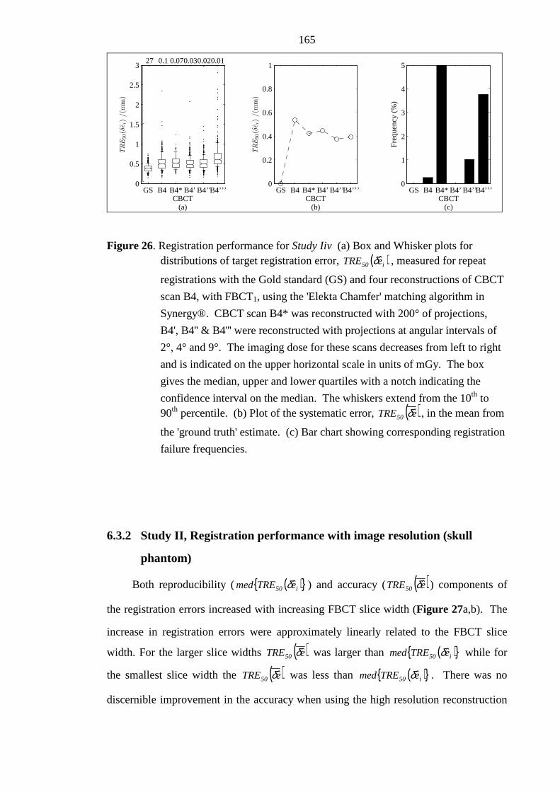
165

GS B4 B4* B4’ B4’’B4’’’0

0.5

1

1.5

2

2.5

3

CBCT(a)

TRE

50(δ

ei)

/(m

m)

GS B4 B4* B4’ B4’’B4’’’0

0.2

0.4

0.6

0.8

1

CBCT(b)

TRE

50(δ

ei)

/(m

m)

GS B4 B4* B4’ B4’’B4’’’0

1

2

3

4

5

Fre

quen

cy (

%)

CBCT(c)

27 0.10.070.030.020.01

Figure 26. Registration performance for Study Iiv (a) Box and Whisker plots for distributions of target registration error, ( )i50 eTRE δ , measured for repeat

registrations with the Gold standard (GS) and four reconstructions of CBCT

scan B4, with FBCT1, using the 'Elekta Chamfer' matching algorithm in

Synergy®. CBCT scan B4* was reconstructed with 200° of projections,

B4', B4'' & B4''' were reconstructed with projections at angular intervals of

2°, 4° and 9°. The imaging dose for these scans decreases from left to right






6.3.2 Study II, Registration performance with image resolution (skull

phantom)

Both reproducibility ( ( ){ }i50 eTREmed δ ) and accuracy ( ( )eTRE50 δ ) components of

the registration errors increased with increasing FBCT slice width (Figure 27a,b). The

increase in registration errors were approximately linearly related to the FBCT slice

width. For the larger slice widths ( )eTRE50 δ was larger than ( ){ }i50 eTREmed δ while for

the smallest slice width the ( )eTRE50 δ was less than ( ){ }i50 eTREmed δ . There was no

discernible improvement in the accuracy when using the high resolution reconstruction

166

and only a small improvement in the reproducibility component. The relationship of IR

error with FBCT slice width held for both the high dose gold standard scan and the

standard clinical dose CBCT scan A3 but deteriorated for the lowest dose CBCT scan

B4. In particular the systematic errors were greater even for the smallest slice width

FBCT scans.

Registration failures (Figure 27c) were more frequent with registrations using

CBCT scans acquired at the lowest dose and larger voxel size although the probability

of failure was less than or equal to 1% for all image pairs.

6.3.3 Study III, registration performance with patient im ages

The random component of the registration errors for patients performed with a CT

slice width of 5 mm (average ( ){ }i50 eTREmed δ = 0.75 mm) were approximately 50%

greater than those performed with a 2.5 mm slice width (average ( ){ }i50 eTREmed δ = 0.50

mm). This compares with 0.33mm for the 2.5mm slice width (CT4-CBCTA3(S)) and

0.41mm, for the 5mm slice width (CT5-CBCTA3(S)) measured with the skull phantom

data.

The third scan of patient four exhibited an unusually high random registration

error ( ( ){ }i50 eTREmed δ = 1.2 mm). The 90th percentile ranges were 0.75 mm to 2 mm.

The frequency of registration failures, ( ) 5.2eTRE i50 >δ mm, ranged from 0 to 2.5% for

all but one FBCT-CBCT scan pair which was 7% (Figure 28a). Registration failures

only occurred if InitialTRE was greater than 10 mm (Figure 28b).

The measured ( )i50 eTRE δ data was plotted against the initial misalignment,

expressed as a target registration error using the method described previously. This

showed that registration failures were more frequent and the spread of ( )i50 eTRE δ

became larger as the initial misalignment increased (Figure 29).

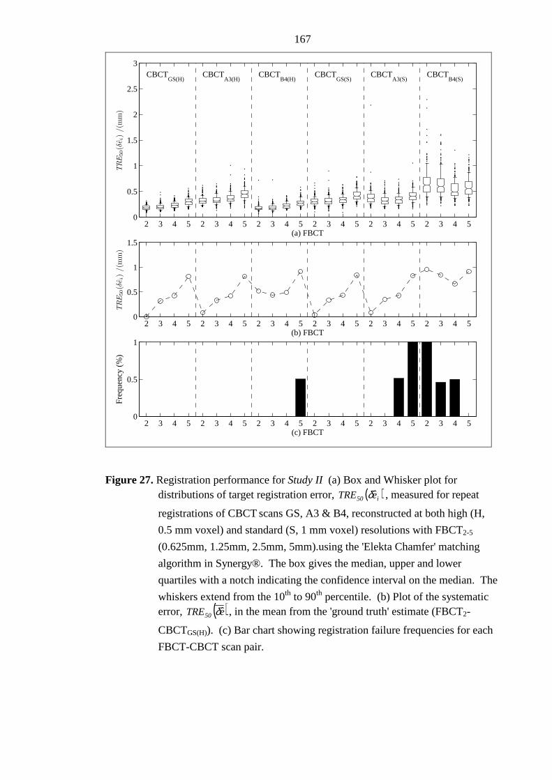
167

2 3 4 5 2 3 4 5 2 3 4 5 2 3 4 5 2 3 4 5 2 3 4 50

0.5

1

1.5

2

2.5

3

TRE

50(δ

ei)

/(m

m)

(a) FBCT

CBCTGS(H)

CBCTA3(H)

CBCTB4(H)

CBCTGS(S)

CBCTA3(S)

CBCTB4(S)

2 3 4 5 2 3 4 5 2 3 4 5 2 3 4 5 2 3 4 5 2 3 4 50

0.5

1

1.5

TRE

50(δ

ei)

/(m

m)

(b) FBCT

2 3 4 5 2 3 4 5 2 3 4 5 2 3 4 5 2 3 4 5 2 3 4 50

0.5

1

Fre

quen

cy (

%)

(c) FBCT

Figure 27. Registration performance for Study II (a) Box and Whisker plot for distributions of target registration error, ( )i50 eTRE δ , measured for repeat

registrations of CBCT scans GS, A3 & B4, reconstructed at both high (H,

0.5 mm voxel) and standard (S, 1 mm voxel) resolutions with FBCT2-5

(0.625mm, 1.25mm, 2.5mm, 5mm).using the 'Elekta Chamfer' matching

algorithm in Synergy®. The box gives the median, upper and lower

quartiles with a notch indicating the confidence interval on the median. The

whiskers extend from the 10th to 90th percentile. (b) Plot of the systematic error, ( )eTRE50 δ , in the mean from the 'ground truth' estimate (FBCT2-

CBCTGS(H)). (c) Bar chart showing registration failure frequencies for each

FBCT-CBCT scan pair.

168

A uniform distribution of initial misalignments with translations up to 40mm and

rotations up to 20° was chosen to measure the performance of the IR algorithms well

beyond the normal range of clinical operation. Typical initial misalignments are much

less in clinical practice than tested in this study. To determine more clinically realistic

estimates of registration uncertainties, the data presented here were sub-sampled to

reflect a distribution that was more typical of patient set-up errors found in clinical

practice, i.e. independent translations, distributed normally (σ = 3 mm), and rotations

about an axis of random orientation, also distributed normally (σ = 3°). For the IRs

performed on the patient data in this study, 90% of all registrations had a ( )i50 eTRE δ less

than 1 mm. When this error was separated into individual components along the

patient’s cranial–caudal, anterior–posterior and lateral directions, the standard deviation

of each component was found to be approximately 0.4 mm. Whilst this error is small it

should nevertheless be considered when designing CTV–PTV margins for IGRT

protocols especially if the protocol involves online correction on each fraction and the

number of fractions is small.

6.3.4 Study IV, Registration uncertainty with clipbox position (patient

images)

The random and systematic IR components showed a relatively low sensitivity to

clipbox position (Figure 30). For the three CBCT scans used in this study the range of

( ){ }i50 eTREmed δ values was no greater than 0.3mm. Given an IR result using one of the

clipboxes there was an equal probability of improving and degrading the registration

with a minor adjustment of the clipbox.

169

1 2 3 1 2 3 1 2 3 1 2 3 1 2 3 1 2 3 1 2 30

0.5

1

1.5

2

2.5

3

3.5

4

4.5

TRE

50(δ

ei)

/(m

m)

CBCT(a)

Patient 1FBCT = 5mm

Patient 2FBCT = 5mm

Patient 3FBCT = 5mm

Patient 4FBCT = 5mm

Patient 5FBCT = 2.5mm



1 2 3 1 2 3 1 2 3 1 2 3 1 2 3 1 2 3 1 2 30

2

4

6

8

Fre

quen

cy (

%)

CBCT(b)

Figure 28. Registration performance for Study III (a) Box and Whisker plot for distributions of target registration error ( )i50 eTRE δ measured using seven

patient head images. Each bar represents repeat registrations of one of three

CBCT scans with the respective patient's FBCT scan using the 'Elekta

Chamfer' image registration algorithm in Synergy®. The box gives the

median, upper and lower quartiles with a notch indicating confidence

interval on the median. The whiskers extend from the 10th to 90th percentile.

(b) Bar chart showing corresponding registration failure frequencies.

170

0 5 10 15 20 25 30 35 400

10

20

30

40

50

60

70

80

90

100

TRE

50(δ

ei)

/(m

m)

TREInitial

(a)

Figure 29. Study III, Plot of measured registration error, ( )i50 eTRE δ against applied

misalignment, InitialTRE for all patient data. The horizontal dotted line

represents the threshold value of ( ) 5.2eTRE i50 =δ above which registrations

were classified as failures.

171

0

0.5

1

1.5

2

2.5

3

3.5

4

4.5

TRE

50(δ

ei)

/(m

m)

FBCT−CBCT pair(a)

Patient 1 Patient 2 Patient 3

0

5

10

Fre

quen

cy (

%)

FBCT−CBCT pair(b)

Figure 30. Registration performance for Study IV (a-c) Box and Whisker plot for distributions of target registration error ( )i50 eTRE δ measured for repeat

registrations of CBCT scans for one fractions each of the first three patients

using the 'Elekta Chamfer' image registration algorithm in Synergy®.

Repeat registrations were executed 20 times for each image pair using 20

randomly sampled clipbox positions. The box gives the median, upper and

lower quartiles with a notch indicating confidence interval on the median.

The whiskers extend from the 10th to 90th percentile. (b) Bar charts showing

corresponding registration failure frequencies.

172

6.3.5 Study V, Registration performance after multiple image registrations

(patient images)

When IR was repeated using the result of the first IR as the starting point of the

second, there was a small effect on the IR performance. A simple analysis would

suggest the distribution of the random component was unchanged (Figure 31a) and the

number of failures reduced to zero (Figure 31b). A paired analysis (Figure 32a)

showed that overall, 63% of IRs were improved by an average of 0.3mm which is not

significant in clinical terms. However, for the 12 (out of 600) registrations where

( )i50 eTRE δ was originally greater than 2.5 mm, 10 had a ( )i50 eTRE δ of less than 2.5 mm

after a second registration. Only 2 out of the 6 which had a ( )i50 eTRE δ > 5mm after the

first registration were not improved to ( )i50 eTRE δ < 2.5mm. This shows that a second

registration can be beneficial.

6.3.6 Study VI, Registration performance with the grey value matching

algorithm (patient images)

The random component of IR errors, performed with the 'Elekta Correlation Ratio'

IR algorithm ( ( ){ }i50 eTREmed δ = 0.05mm) were more than a factor of 10 less than with

the 'Elekta Chamfer' algorithm ( ( ){ }i50 eTREmed δ = 0.7mm (Figure 31a) but the number

of registration failures increased to between 6.5 and 8.5% (Figure 31b). A paired

analysis (Figure 32b) showed that overall, 91% of IRs were improved. Of the 12

registrations which were greater than 2.5 mm with a single 'Elekta Chamfer' match, 10

were improved to ( )i50 eTRE δ < 2.5 mm. However, of the other 588 for which,

( )i50 eTRE δ , was previously less than 2.5 mm, 43 became > 2.5 mm with the 'Elekta

Correlation Ratio' algorithm. The lowest InitialTRE for which ( )i50 eTRE δ was greater

than 2.5 mm was 13mm which is similar to that of the 'Elekta Chamfer' algorithm. This

was at the expense of increased time as the 'Elekta Correlation Ratio' registration

algorithm took up to 4 minutes to complete while the 'Elekta Chamfer' algorithm took

less than 5 seconds.

173

6.3.7 Study VII, Effect of image re-sampling (patient images)

There was a small but significant difference in the random components of the IR

errors if the initial misalignment was created using the graphical user interface of the

XVI application software (Figure 31a,b). For all registrations ( )i50 eTRE δ < 2.5mm (i.e.

excluding outliers), a paired t-test showed there was a small (0.07mm) but significant

difference in the means (P < 10-5, excluding registrations with ( )i50 eTRE δ > 2.5mm)

(Figure 32c). The re-sampled registrations had the larger ( )i50 eTRE δ . The average

( ){ }i50 eTREmed δ for study VII was 0.65mm compared with 0.7mm for study III. The

average failure frequency ( ( )i50 eTRE δ > 2.5 mm) was 3 % with this method compared to

2% if the image is re-sampled (Study III). This small difference indicated that image re-

sampling was unnecessary in order to get a reasonable estimate of random IR

uncertainties.

174

III V VI VII III V VI VII III V VI VII0

0.5

1

1.5

2

2.5

3

3.5

4

4.5

Study(a)

TRE

50(δ

ei)

/(m

m)

Patient 2: FBCT−CBCT(1) Patient 2: FBCT−CBCT(2) Patient 2: FBCT−CBCT(3)

III V VI VII III V VI VII III V VI VII0

2

4

6

8

10

Study(b)

Fre

quen

cy (

%)

Figure 31. Registration performance for Studies V, VI & VII (a) Box and Whisker plot for distributions of target registration error ( )i50 eTRE δ measured for repeat

registrations of CBCT scans with CT data for three fractions of patient 2.

The results for study III, performed with the 'Elekta Chamfer' algorithm are

compared with the alternative methods of studies V, VI and VII. In study V,

the 'Elekta Chamfer' registration was run twice. Study VI used the 'Elekta

Correlation Ratio' registration algorithm and study VII used an alternative

method of initial image misalignment. The box gives the median, upper and

lower quartiles with a notch indicating confidence interval on the median.

The whiskers extend from the 10th to 90th percentile. (b) Bar chart showing

corresponding registration failure frequencies.

175

0 10 20 30 40 500

20

40

60

80

100

120

TRE50(δei) for study III (mm)(a)

TRE

50(δ

ei)

for

study

V(m

m)

0 10 20 30 40 500

20

40

60

80

100

120

TRE50(δei) for study III (mm)(c)

TRE

50(δ

ei)

for

study

VII

(mm

)

0 2 40

1

2

3

4

5

0 10 20 30 40 500

20

40

60

80

100

120

TRE50(δei) for study III (mm)(b)

TRE

50(δ

ei)

for

study

VI(m

m)

0 2 40

1

2

3

4

5

0 50

1

2

3

4

5

Figure 32. Correlation between registration uncertainties for Studies V, VI & VII

Results for study III performed with the Elekta Chamfer' algorithm

compared with the alternative methods of studies V, VI and VII. In study V,

the 'Elekta Chamfer' registration was run twice. Study VI used the 'Elekta

Correlation Ratio' registration algorithm and study VII used an alternative method of initial image misalignment. (a-c) ( )i50 eTRE δ for each of the

methods plotted against ( )i50 eTRE δ for study III. The inset for each of these

plots has an expanded scale indicated by the dashed box on the main plot.

176

6.4 Discussion

In a previous feasibility study [4], IR was shown to be highly accurate for CT-

CBCT image pairs of a skull phantom and was robust to reduction of the imaging dose.

The study used a voxel intensity based IR algorithm using a global correlation cost

function in a treatment planning system and not the algorithms provided in the Elekta

Synergy® system. This study also relied on manually repeating IR which limited

sample sizes and therefore the ability to assess registration uncertainties. In the follow-

on study, presented in this chapter, the performance of the IR algorithm in a commercial

IGRT system was assessed using up to 200 randomly sampled misalignments with the

aid of Windows scripting software. This enabled a much more comprehensive analysis

of IR uncertainties.

A further deficiency in the earlier study of Sykes et al. [4] was the use of the

Alderson Rando phantom. The Rando phantom was not an ideal choice for an IR study

as it was made up of 3 cm thick slices each containing many cylindrical inserts to enable

placement of small dosimeters. These would have been visible in both FBCT and

CBCT images and could, therefore, have influenced the registration accuracy. In the

current study a skull phantom was used which did not possess structures that could

influence the accuracy of IR.

The imaging dose was reduced as far as practically possible by using a

combination of copper attenuators and reduced projection images in reconstruction. The

'Elekta Chamfer' algorithm was found to be very robust to a reduction in imaging dose

by either method. This is a significant finding, particularly for paediatric patients where

the concomitant imaging dose of repeat CBCT required for accurate setup is of concern.

Registrations with CBCT scan A1 showed elevated systematic and random error

components ( ( )eTRE50 δ = 0.7mm, ( ){ }i50 eTREmed δ = 0.5mm). This may have been due to

the high exposure of which was sufficient to saturate the imager external to the

177

phantom. This caused greater in-homogeneity in the grey level for regions of the

phantom that had uniform density. Over-exposure and saturation of the imager which

increased the registration uncertainty for registrations with CBCT scan A1 could be

avoided with use of the bow-tie filter, now supplied by the manufacturer.

While the increase in systematic and random uncertainties of IR with increasing

FBCT slice width and CBCT voxel size was expected, the results show there is little

benefit in reducing CT slice width less than 2.5mm or reconstructing the CBCT images

at (0.5mm)3 instead of (1mm)3. The patient data also supports the reduction of FBCT

slice width to less than 5mm to ensure the majority of random errors are less than 1mm.

The exact placement of the Clipbox boundaries was not found to be critical with

larger gains to be found if the IR was performed a second time. This information

provides practical guidance to operators of the XVI application regarding the relative

merits of adjusting the Clipbox or repeating the automatic IR compared to manual

adjustment of the registration.

The majority of IR errors were dominated by the translational component. The

ratio of ( )i50 eTRE δ calculated on the translational component alone to the ( )i50 eTRE δ for

both rotation and translation was 0.76 for more than 90% of registrations in study III .

In the first part of a study by Meyer et al. [74] investigating the positioning errors

associated with CBCT, initial misalignments and hence the starting point for automatic

IR were achieved by incrementing the coordinates of the treatment plan centre by

0.1mm and 0.5mm in the x, y & z directions. The Synergy® system used the

coordinates of the planned treatment centre in the CT frame of reference in order to

initially align the CBCT scan with the CT scan. The 'Elekta Correlation Ratio'

registration algorithm was able to exactly detect the 0.1mm displacements of the

treatment centre while the 'Elekta Chamfer' algorithm gave small errors, less than

0.3mm and 0.4°. Their method did not allow the effect of rotational misalignment on IR

to be measured. In this chapter, the random component of the registration errors with

178

the 'Elekta Correlation Ratio' were found to be predominantly less than 0.1mm. This is

in broad agreement with the work of Meyer et al. For the 'Elekta Chamfer' algorithm,

95% of all registrations were within ±0.8mm in each direction and with a combined

rotation of less than 1.4°. These measurements are larger than those found by Meyer et

al. but this maybe due to the inclusion of an initial rotational misalignment in the

methods used in this chapter.

The re-sampling and sub-pixel interpolation of the CBCT image when transformed

in this study would not have exactly replicated a real shift of the phantom or patient.

Structural noise and image artefacts would also have been transformed and re-sampled

along with the image data whereas, in reality, these are more likely to have a fixed

position in relation to the imager or to change characteristics according to the position

and orientation of the subject. However, study VII, showed, for the 'Elekta Chamfer'

algorithm, that reasonable estimates of IR uncertainties may be achieved if the initial

misalignment is created by just changing the starting point for IR without interpolation.

This suggests that image interpolation is not critical for these measurements and has the

added advantage of significantly reducing the computational overhead.

Chamfer matching relies on edge detection of the bony anatomy surface. The very

low dose reconstructions of the head phantom had significantly increased CT values. It

was thought that this could affect the segmentation process leading to the phantom

surface being extracted instead of the bony anatomy. A set of CT images simulating the

low dose scans was created having removed the phantom surface to air interface using

image processing techniques. Repeat registrations gave similar results to the original

images showing that the Chamfer matching algorithm was extracting the correct surface.

One effect of using copper attenuators to simulate lower dose scans is beam

hardening which can lead to a cupping artefact although this was not strongly evident in

the images acquired for this study. However, the mean grey-level did increase with

increasing copper thickness. This may have been the cause of the increased registration

errors with the greatest thickness of copper. Despite the possibility of the copper

179

attenuator affecting registration performance registration errors did not deteriorate

rapidly. This indicates that imaging dose can be reduced, below that available in normal

operation of the equipment, without significantly compromising the performance of the

investigated automatic IR algorithms.

A uniform distribution of initial misalignments with translations up to 40mm and

rotations up to 20° was chosen to measure the performance of the IR algorithms beyond

the normal range of clinical operation. Since the typical initial misalignments will be

much less in clinical practice than tested in this study, and the registration uncertainties

appeared to be linearly related to the magnitude of the initial misalignment, the

registration uncertainties presented here will be an over estimate. To determine more

clinically realistic estimates of registration uncertainties the data presented here was

sub-sampled to reflect a distribution that was more typical of patient set-up errors found

in clinical practice i.e. independent translations distributed normally (σ=3mm) and

rotations about an axis of random orientation also distributed normally (σ=3°). For the

IRs performed on the patient data in study III, 90% of all registrations had a ( )i50 eTRE δ

less than 1.3 mm. When this error was separated into individual components along the

patient's cranial-caudal, anterior-posterior and lateral directions, the standard deviation

of each component was found to be approximately 0.5 mm. Whilst this error is small it

should nevertheless be considered when designing CTV-PTV margins for IGRT

protocols especially when the protocol involves online correction on each fraction.

In this study the ( )i50 eTRE δ parameter of IR performance was proposed. The

'Elekta Chamfer' match algorithm utilised in the Synergy® system was based on the

Chamfer match algorithm implemented by van Herk and Kooy, [111]. Analysis of IR

errors in this and a later study [190] were performed in a similar manner to the methods

used here. The set of points used to define ( )i50 eTRE δ in their study were those extracted

from the surface of the skull in the CT image in order to perform the Chamfer match.

Since these points were not available for this study, ( )i50 eTRE δ was calculated from the

displacement of a set of points on the surface of a sphere centred on the isocentre. This

180

had the advantage of being independent from the algorithm. Furthermore the sphere

was centred on the isocentre which is typically the centre of the treatment volume and

the centre of rotation of the moving image in the IR.

A number of authors have addressed the quality assurance of IR algorithms for

both radiotherapy treatment planning and image guidance. The methods employed are

wide ranging and include use of various phantoms and methods of visual assessment.

As demonstrated in this study the use of phantoms can underestimate the typical IR

errors. Physical displacement of the phantoms is limited by both the time taken to

perform each measurement and the precision that the phantom can be displaced

[137,139]. Visual assessment is limited by both the subjective nature of the observer

and the time taken to assess each registration. Identification of corresponding fiducial

points on 3D images is also prone to error as features that can be pinpointed in a 2D

sectional plane are rarely well defined perpendicular to the plane [132,187]. The

number of corresponding points that can be readily defined is also a limiting factor.

Many studies published on IR performance have been performed by the developers of

the algorithm and bench marked against other established algorithms [116,119]. Access

to source code makes automation of the process relatively straightforward but does not

test the commercial implementation in the clinical setting. This is an important factor if

decisions about clinical processes are to be formed on the basis of understanding IR

performance.

181

6.5 Conclusions and Future Work

6.5.1 Conclusions

In this chapter, methods of measuring the IR performance of a commercial IGRT

system have been developed. These methods have been applied to the study of IR

accuracy, precision and robustness for image guidance of intra-cranial tumours based on

IR of the bones of the skull with the 'Elekta Chamfer' algorithm. With the skull

phantom the accuracy, in terms of TRE50 , was significantly less than 0.5mm for CT

slice widths less than or equal to 2.5mm. The precision (reproducibility), based on

patient images, was such that the TRE50 was less than 1.3 mm for 90% of patients if the

initial patient set-up errors were typical i.e. normally distributed with σtranslation= 3mm

and σrotation = 3°. This equates to a standard deviation of 0.5mm for individual lateral,

cranial-caudal and anterior-posterior random error components of target registration

error on the surface of a 50mm radius sphere. The algorithm was also robust with no

registration failures for initial setup errors of this magnitude. This indicates the

performance of the algorithm is suitable for image guidance of intra-cranial tumours. It

also suggests that a thorough visual check of alignment might not be required before

treatment. The precision of the 'Elekta Correlation Ratio' algorithm was better than the

'Elekta Chamfer' algorithm however this was at the expense of increased computational

time and reduced robustness.

The limit at which IR performance started to deteriorate rapidly (with decreasing

image dose) was not found with the range of imaging doses investigated in this study.

There was a slight deterioration for imaging doses less than 0.4 mGy but no further

deterioration for doses down to 8 µGy. Since even a dose of 0.4mGy is very low in the

context of the dose received by the patient from radiotherapy it would seem unnecessary

to reduce the dose further. Hence, a dose of 0.4mGy could be considered as optimum.

182

This is a factor of ten lower than that which can be set under normal operation of the

clinical system.

6.5.2 Future Work

Given the results of this chapter, it is likely that the benefits of low registration

failures of the 'Elekta Chamfer' algorithm and greater precision (reproducibility) of the

'Elekta Correlation Ratio' algorithm can be combined if the 'Elekta Chamfer' algorithm

were to be applied immediately prior to the 'Elekta Correlation Ratio' algorithm. It is

also likely that the number of iterations required for the 'Elekta Correlation Ratio'

algorithm would be low given a good starting point from the 'Elekta Chamfer' algorithm

thereby reducing the overall computation time when compared to the 'Elekta Correlation

Ratio' algorithm alone. The hypothesis that the combination of the two algorithms

provides better overall performance than either of the algorithms used individually

should be tested.

Image guidance based on bony anatomy is also used in treatment of other clinical

sites such as, mediastinal lung, oesophagus, and head and neck tumours. Quantification

of the precision and robustness of IR in these sites would determine the benefits of

employing automatic IR in these sites.

Chapter 7

Measurement of automatic image registration

uncertainties for prostate tumours: pelvis

phantom and patient FBCT and CBCT images

7.1 Introduction

In chapter 6, the technique for investigating image registration (IR) uncertainties

was established and utilised on FBCT and CBCT images of a skull phantom and patient

head images, primarily using the 'Elekta Chamfer' algorithm. The high contrast of the

bone to soft tissue interfaces makes this a fairly robust process to the extent that the

algorithm did not fail catastrophically even when the imaging dose was reduced to very

low levels. In part II, the same techniques are used to investigate the more challenging

IR problem of soft tissue matching of the prostate.

The robustness of the Correlation Ratio IR algorithm was studied by the

developers of the XVI software. In their study [88], performed on a non commercial

version of the algorithm, IR of the prostate were evaluated visually by one experienced

observer. The clinical target volume which in their case was the prostate, not including

seminal vesicles was expanded by 3.6mm to create a set of verification contours. These

contours were overlaid on the CBCT image. The observer's task was to determine if any

part of the prostate in the CBCT image was outside the verification contours.

184

In this chapter the analysis of IR errors was designed specifically to allow a

reasonable comparison with the frequency of registration failure measured by

Smitsmans et al. In addition, in this chapter, the accuracy, reproducibility and robustness

are investigated as a function of imaging dose using an anthropomorphic phantom of the

pelvis and patient images are used to determine precision and robustness of automatic

IR in clinical practice.


In this study the basic methods of performing repeat IR having first transformed

the CBCT image data to one of a random selection of rigid body transforms was the

same as in chapter 6. The methods differed slightly due to the availability of a new

treatment couch on the Synergy® system that allowed patient positioning with six dof

i.e. translation and rotation. The Hexapod® evo system (Elekta AB, Sweden,

Stockholm) which was the subject of investigations in Chapter 5 was able to position

the phantom more accurately to match the position in the FBCT scan and therefore

reduce any systematic errors to a minimum. The study also required a newer version of

the XVI software. In the XVI version 4.2 studied in Chapter 6, it was impossible to set

the clipbox so that bony anatomy and air in the rectum of the FBCT scan were excluded

whilst keeping the prostate and seminal vesicles within the volume. The newer XVI

version 4.5 software, which was released in spring 2010, but was not available during

the time of this study, enabled a masked region of interest to be defined based on the

reference FBCT scan. Only image data within the mask was used by the IR algorithm.

This enabled the user to define a mask containing just the prostate and a small amount

of surrounding tissue whilst excluding bone and the rectum. With knowledge of this

development a research version of the XVI software was acquired from the software

developers based at the Netherlands Cancer Institute (NKI, Amsterdam, Netherlands) in

order to perform this investigation. The research version was effectively a Beta release

185

of the commercial release with some extra tools written specifically to enable the work

in Chapter 8 [191].

7.2.1 FBCT and CBCT imaging

7.2.1.1 Phantom Imaging

A CIRS Model 801 P-F phantom otherwise known as the Virtually Human Male

Pelvis Phantom or VHMP was scanned on a Siemens Sensation Open 24 CT scanner

with 1.5 mm slice thickness and inter-slice spacing of 1mm. The trans-axial plane pixel

size was approximately 1mm. Using the Advantage Sim™ MD application (v7.6) the

patient surface, GTV (prostate and seminal vesicles), bladder, rectum and pelvic bones

were either auto-segmented or delineated manually. A single anterior beam was added

with isocentre aligned to the lateral and anterior positions of the middle plane of CT

markers. This coincided approximately with the geometric centre of the prostate. The

plan was sent to the Synergy® system in preparation for CBCT imaging.

The phantom was aligned on the Hexapod treatment couch of the Synergy®

system according to the room lasers and the fiducial markers (2.3mm Beekley SPOTS)

placed at the time of CT scanning which indicated the isocentre position approximately.

An initial CBCT image was acquired and IR performed using the 'Elekta Chamfer'

algorithm with the FBCT reference markers including the majority of the pelvic bones

in the registration Clipbox. The three translation and three rotation transformation

parameters resulting from the IR were used to drive the Hexapod couch to eliminate all

translation and rotation positioning errors. A second CBCT was performed to verify the

position to within 0.05mm and 0.05°. All CBCT imaging was performed at a tube

voltage of 120kV with a 360° rotation of the scanner using the medium field of view

(40cm diameter) and coned to an approximate 13 cm length. Seven scans were

performed with a range of exposure settings (Table 11) Images were reconstructed at

medium resolution i.e. with a cubic voxel dimension of 1mm.

186

Table 11. Exposure settings for the seven scans A-G and a measurement of nominal scan dose measured in a CTDI phantom with a Farmer chamber.

Scan Label Tube Current (mA0

Pulse Length (ms)

Total exposure (mAs)

CTDI Dose (mGy)

A 40 80 2176 39.8

B 40 50 1360 24.9

C 32 40 870.4 15.9

D 12 80 652.8 11.9

E 25 20 340 6.2

F 25 12 204 3.7

G 10 10 68 1.2

7.2.1.2 Patient Imaging

Six patients were sampled from a clinical database of the Synergy® system. The

first three CBCT images were sampled from each patient. The CT slice thickness and

slice separations were both 5mm and trans-axial plane pixel size was approximately

1mm.

CBCT scans were all performed with medium field of view collimated to a 13cm

length. The tube voltage was 120kV and the tube exposure settings were the same as

scan D for the phantom. The scans were reconstructed at medium resolution.

7.2.2 Image Registrations

Image registrations were performed using a research release of the XVI software.

An IR mask was created based on the GTV (prostate and seminal vesicles), previously

delineated by a radiologist for the patient's treatment, with a 5mm expansion in all

directions. The 5mm expansion was necessary to include gradients in CT number at the

periphery of the prostate. The mask was then edited manually to ensure that neither air

pockets nor pelvic bones in the FBCT image of the rectum were included.

187

Repeat IR were performed for each FBCT-CBCT scan pair and the rigid body

transform parameters recorded. For each FBCT-CBCT scan pair, one hundred repeat

registrations were performed with the CBCT scan misaligned using the ITK

Versor3DRigidBody class as described in chapter 6. The range of translations and

rotations sampled for misalignment of the skull images in part I proved to be too great

for the registration of the prostate. This is not surprising as the diameter of the prostate

is only 5 cm. Consequently a more realistic set of transforms was calculated by

sampling a normal distribution with the standard deviations reported by Stroom et al

[192]; which are translations: σLR = 0.06, σAP = 0.28, σSI = 0.28 and rotations: σLR =

3.4, σAP = 0.9, σSI = 1.6. These represent the random error of the prostate motion

relative to the bony anatomy for patients in the supine position.

All IR were performed with the 'Elekta Correlation Ratio' IR algorithm. The

general method for analysis of the IR transform results was performed as described in

chapter 6 but with a few changes. The reason for these changes was to create a similar

criteria for failure as that used by Smitsmans et al [88] i.e. no part of the prostate

boundary should be misaligned by more than 3.6mm. First, the TRE was calculated at a

radius of 30mm as this is more typical of the prostate dimensions. Secondly, the

maximum target registration error for any of the points on the sphere was calculated

instead of the mean TRE as describe in chapter 4, and finally, the threshold value of

TRE above which an IR was classed as a failure was 3.6mm.

It is also worth noting that a match on bone was not performed first to provide a

good starting point for the soft tissue match of the prostate as performed in the study by

Smitsmans et al. [88]. Since the phantom was rigid an IR of bone would also match the

prostate exactly which would not be the case in a patient where the prostate position

moves relative to the bony anatomy within certain constraints. For this reason, the

initial misalignments were based on the differential motion of the prostate relative to the

bones observed by Stroom et al. [192].

188

7.3 Results

The CBCT scan of the VHMP phantom acquired at the highest dose setting (A)

clearly shows the contrast between soft tissues of the prostate, bladder and rectum with

the surrounding fatty tissues (Figure 33). The image noise increases markedly with

decreasing image dose to the point where no clear border between the prostate and the

lateral fatty tissues was visible (Figure 34).

Figure 33. Transaxial, Sagittal and Coronal sections through CBCT scan A scanned

with the highest dose setting.

189

Figure 34. Transaxial sections of CBCT scans A to G, centred on the prostate, showing

the deterioration of image quality with imaging dose.

The random error component represented by ( ){ }imax30, eTREmed δ , for scans A-E

remained constant at less than 0.2mm with nominal scan doses down to 6.2mGy

(Figure 35a). The frequency of registration failures, defined as ( ) 6.3eTRE imax,30 >δ , was

also less than 5% for these scans (Figure 35c). The systematic error

component ( )eTRE max,30 δ , however, increased steadily between scans A and E with

decreasing dose, rising to a maximum of 0.9mm (Figure 35b). This was still less than

the size of the CBCT and FBCT voxel sizes. For scan F the ( ){ }imax30, eTREmed δ

190

remained at 0.2mm however the frequency of registration failures also rose to near 7%

and the systematic error had risen to 1.5 mm. For the lowest dose scan, G,

( ){ }imax30, eTREmed δ rose to 0.8mm, the systematic error to 2.2mm and the frequency of

errors to 10%. This showed that there was a clear relationship between the scan dose

and the IR error. The scan setting used for patient imaging was based on scan D which

had exposure settings twice that of scan E, the point at which the IR performance starts

to deteriorate.

IR performance for the patient scans did not match that of the phantom scans

except for three FBCT-CBCT scan pairs (Figure 36). There was a large range in

performance with the random component described by ( ){ }imax30, eTREmed δ ranging

between 0.2mm and 9.2mm and with a range of failure frequency between 1% and 88%.

191

A B C D E F G0

5

10

15

Fre

quen

cy (

%)

CBCT(c)

A B C D E F G0

1

2

3

TRE

30,m

ax(δ

ei)

(mm

)

CBCT(b)

39.8 24.9 15.9 11.9 6.2 3.7 1.2

Dose /mGy

A B C D E F G0

1

2

3

4

5

6

7

TRE

30,m

ax(δ

ei)

(mm

)

FBCT−CBCT pair(a)

Figure 35. Soft tissue registration performance for VHMP phantom with decreasing

dose. (a) Box and Whisker plots for distributions of target registration error, ( )imax,30 eTRE δ , measured for repeat registrations of CBCTA-G with FBCT,

using the 'Elekta Correlation Ratio' matching algorithm in the research

version of XVI and a mask set to the GTV + 5mm. The imaging dose for

these scans decrease from left to right and is indicated in the upper

horizontal scale. The box gives the median, upper and lower quartiles with

a notch indicating the confidence interval on the median. The whiskers

extend from the 10th to 90th percentile. (b) Plot of the systematic error, ( )eTRE max,30 δ , in the mean from the 'ground truth' estimate. (c) Bar chart

showing corresponding registration failure frequencies.

192

0

20

40

60

80

100

Fre

quen

cy (

%)

CBCT(b)

0

1

2

3

4

5

6

7

8

9

10

TRE

30,m

ax(δ

ei)

(mm

)

FBCT−CBCT pair(a)

Patient 1 Patient 2 Patient 3 Patient 4 Patient 5 Patient 6

Figure 36. Soft tissue registration performance for the prostate in patient images. (a)

Box and Whisker plot for distributions of target registration error

ieδTRE measured using images from seven prostate patients. Each bar

represents repeat registrations of one of three CBCT scans with the

respective patient's FBCT scan using the 'Elekta Chamfer' IR algorithm in

Synergy®. The box gives the median, upper and lower quartiles with a

notch indicating confidence interval on the median. The whiskers extend

from the 10th to 90th percentile. The horizontal dotted line represents the threshold value of 6.3ˆ =

ieδTRE mm above which registrations were classified

as failures. (b) Bar chart showing corresponding registration failure

frequencies.

193

7.4 Discussion

The VHMP phantom results which show a clear relationship between IR

uncertainty and dose with nominal scan doses less than 6mGy leading to increased

frequency of registration failure. This dose is approximately half the nominal dose for

current clinical scan protocols. This has potential to inform clinical practice and enable

scan doses to be reduced to a minimum without affecting IR. However, the 6mGy cut-

off should be considered carefully as the actual scan dose for patients that are larger than

the VHMP phantom will be lower and therefore higher exposure settings may be

required to maintain automatic IR performance. For these large patients the current scan

exposures setting may not be sufficient for optimal IR performance.

The IR performance with the patient images was disappointing. The patient

CBCT images were generally of poor quality with inadequate definition of the prostate

boundary, particularly at the prostate-rectum and prostate-bladder borders. In some

patients the rectum size had increased greatly from the FBCT scan and in others there

was evidence of intra-scan motion which has led to motion artefacts from the changing

position of the bowel gas as well as increased blurring of the muscle-fat tissue

interfaces. FBCT-CBCT scans pairs for which IR performed well were relatively free of

intra-fraction motion artefacts and the rectum size was similar in both FBCT and CBCT

scans.

In many of the patient FBCT-CBCT image pairs studied, the spread of IR

parameters were so great that the hypothesis that the robust mean described in appendix

A.5 represented the ground truth was false. Closer examination of the data showed that

there were loose clusters of IRs with similar parameters. These were quite widely

separated across the parameter space. An attempt to establish likely candidates for the

ground truth was made using K-means clustering [193] however, it was not possible to

194

deduce with any confidence which of the several candidate means was correct or even

eliminate many of the outliers. For the FBCT-CBCT image pairs exhibiting a wide

range of registration results the confidence in the mean IR parameters on which the

calculation of TRE30,max was based was low and consequently the box and whisker plots

in Figure 36 are merely a qualitative indication that the range of IR errors was large.

Only 6 out of the 17 FBCT-CBCT image pairs have a less than 25% failure rate and

consequently a relatively robust measurement of the mean.

Smitsmans et al. performed IR measurements using the correlation ratio similarity

metric. This algorithm was a research version of the 'Elekta Correlation Ratio'

algorithm on which the commercial Synergy® XVI v4.5 software was based [88]. They

visually assessed the IR of 32 patients and 332 CBCT scans and found 65% of patients

were successfully registered. In their work a registration was successful if the boundary

of the prostate was within a 3.6mm expansion of the CTV. For the untransformed

CBCT scans, studied in this chapter, 12 out of 17 (70%) of scans were registered with

TRE30,max < 3.6mm and when the transformed CBCT scans were included the total

number of successful registrations was 69%. The numbers presented in this chapter are

remarkably similar to those of Smitsmans et al. given the relatively low number of

patients and scans that were studied.

Of the 17 FBCT-CBCT scan pairs studied only 9 had median TRE30,max values

less than 3.6mm and only 4 were such that 90% of all registrations were within 3.6mm.

Given these statistics it is clear that automatic registration cannot be relied on for on-line

image guidance of the soft tissues of the prostate without careful validation by the

operator. This is in contrast to the head data.

In this study a margin of 5mm around the GTV marked by the radiologist was

used. In most cases this included the base of the seminal vesicles. In the research

algorithm used by Smitsmans et al air in the rectum was filtered from the mask

automatically. Here the mask was carefully edited so that the rectum was not included.

The pubic bone and calcifications would also have been removed from the mask if they

195

had been present following the advice of Smitsmans et al. However, this was not

necessary.

For some CBCT images automatic IR may give acceptable results however, for the

majority, automatic IR will fail and manual registration will be required. For many of

the images there was evidence of motion during the scan with artefacts from the tissue–

air interfaces that have moved and blurring. This made visual identification of the soft-

tissue boundaries of the prostate and surrounding structures very difficult. In some

cases even the anterior rectal wall which is a good indicator of a prostates anterior-

posterior position was not well defined. In these cases manual IR would also have been

difficult and subject to greater uncertainty. Consequently, the value of CBCT may not

be one of accurate image guidance but more an indicator for when intervention is

required to reduce the likelihood of rectal gas movements. The use of dietary advice,

laxatives, antiflatulents or enemas may be necessary.

7.5 Conclusion

IR of FBCT-CBCT images of the VHMP phantom have demonstrated a clear cut-

off point of 6mGy below which the likelihood of IR failures increases. IR with the

patient images was considerably less robust with large registration uncertainties and

high failure rates. Automatic IR should not be used in the image guided process for

prostates without verification by means of a visual check before treatment.

7.6 Future work

The patient images used in this study were acquired in the first year of

implementation of IGRT at Leeds. Since then several improvements have been

introduced that could lead to better IR performance. Based on the observations of rectal

dimensions and presence of gas, patients are now given better dietary advice and

interventions such as the use of laxatives, antiflatulents and enemas are used when

196

necessary. This has led to better control of rectal fill state. FBCT slice widths have

been reduced to 2.5mm since the images used in this study were acquired which will

almost certainly reduce the likelihood of systematic IR errors. Finally, CBCT image

quality has also improved with the introduction of the bow-tie filter [194] leading to

improved ‘contrast to noise’ ratio and reduced scatter. These changes point to the need

for a repeat study with patient images acquired more recently.

It was noticed that in some cases small edits of the mask could greatly affect the

IR result particularly in the region of the seminal vesicles. Further investigation of the

optimal mask shape and size would determine if the robustness and precision of the IR

algorithm can be improved.

197

Chapter 8

Image registration quality likelihood metrics

based on similarity metric surface shape

8.1 Introduction

In chapters 6 and 7 image registration (IR) uncertainties were measured for

registration of the skull and the prostate. One of the motivations for understanding the

registration uncertainties, the random component in particular, was to determine the risk

of trusting the result of the algorithm implicitly before correction of patient position.

This would be of benefit to image guided radiotherapy using on-line correction

protocols i.e. where patient position is always corrected for any significant misalignment

before treatment commences. The clinical risk of trusting the result would be low if the

spread of registration errors is small relative to the patient set-up error or organ motion

that is being measured. The frequency of IR failures would also have to be sufficiently

small for the clinical risk to be acceptably low. The benefit of accepting the risk would

be a decrease in the amount of time required to perform a visual check before

commencing with treatment. This could lead to a consequent increase in patient

throughput and reduction in the cost of treatment. Furthermore the reduction in time

between imaging and treatment will reduce the frequency and magnitude of errors due to

intra-fraction motion.

198

In Figure 28 of Chapter 6 a threshold of 2.5mm was used to distinguish between

registration successes and failures. This was based on 90% of all registrations having a

TRE50 < 2.5mm for individual initial misalignments distributed normally with a

standard deviation of 1mm and 0.5° respectively. A short, single observer, study was

also performed to determine a value of TRE50 above which registrations were classed as

unacceptable. With only a cursory view of the image alignment the operator did not

classify any registrations with a TRE50 < 2.5 mm as unacceptable ('Poor'). In the same

study the operator found that no misalignment was observed for registrations with

TRE50 < 0.6 mm ('Good'). For registrations with TRE50 between 0.6mm and 2.5mm,

classed as 'OK' i.e. not Good but clinically acceptable the operator would be tempted to

make manual adjustments even though they may not be necessary. To assist the

operator in deciding if further improvement of the IR is necessary a user feedback

metric from the IR would be beneficial.

In this chapter we first investigate the shape of both the Chamfer match and

Correlation Ration similarity metrics (SM) (see section 2.4.1) to determine whether

differences in the characteristics of the SM surface in the vicinity of the global

minimum would indicate whether an IR is likely to be 'Good' , 'OK', or 'Poor'. These

characteristics can be described in terms of a number of evaluation metrics based on

those previously described by Skerl et al [171]. We then show that these metrics can be

used to classify the goodness of an IR according to the measured TRE50 as in Chapter 6.

Furthermore we show that evaluation metrics based on the SM calculated at just a few

locations of the rigid body parameter space, in the vicinity of the transform parameters

returned by the IR, can be used to provide feedback to the user on the likely quality of

an IR.

199


8.2.1 Phantom and patient data

The images for seven patients previously treated with radiotherapy were used in

this study. Images for each patient included the reference FBCT image and three CBCT

images. These were the same images that were used for studying registration

uncertainties in Chapter 6.

8.2.2 Sampling the similarity metric

8.2.2.1 Pre-release XVI v4.5 research mode

The parameter space of the SM was sampled in the vicinity of the transform found

by IR of a FBCT-CBCT pair using a special research release of the XVI application.

This version provided by van Herk (Netherlands Cancer Institute/Antoni van

Leeuwenhoek Hospital - NKI/AvL) [191] was based on software developed at NKI/AvL

in preparation for the commercial release of XVI v4.5 early in 2010. As with version

4.2 of the software, investigated in Chapters 6 & 7, two IR algorithms were available

which employed the Chamfer and Correlation Ratio similarity metrics respectively. The

software was adapted by van Herk to read in a sequence of three translation and three

rotation offsets from a data file. The software applied these offsets to the respective

rigid transform parameters determined from a previous IR and the SM was calculated at

this new rigid body transform location. This was repeated for each offset in the data

file. The SM for each rigid body transform was exported to a second data file.

8.2.2.2 Sampling of the rigid body transform parameter space

In this study the data file of transform parameter offsets was created by sampling

profiles along the six cardinal axis of the parameter space. The offsets for translations

were equally spaced at intervals of 0.2mm between ± 10mm and thereafter at intervals

of 1.6mm out to ± 80mm. The offsets for rotations were equally spaced at intervals of

200

0.05° between ± 5.5° and at intervals of 0.4° out to ± 45°. Since the profiles were along

the parameter axis the order of rotation was not important and therefore it was not

necessary to sample the space using rotation versors and then convert to the Euler angle

rigid body system used by the Synergy® system. A scale factor of approximately 40

between increments of rotation and increments of translation was set empirically so that

the width of the SM's global minimum along all cardinal axes was approximately equal.

8.2.2.3 Sub-sampling registration uncertainty datasets based on TRE50 value

In chapter 6 results of registration uncertainty were presented for IRs using the

commercial release 4.2 of the XVI software. Since this study was performed with the

special pre-release of version 4.5 of the commercial XVI software it was necessary to

repeat the study of IR uncertainties with this version. The SM was analysed for only a

sub-set of the 200 IRs performed with each FBCT-CBCT scan pair. The registrations

were grouped on the basis of their TRE50 values. The registration with the lowest

TRE50 was selected along with six registrations, selected randomly, with TRE50 in each

0.5mm interval between 0 and 4mm. Finally, six with TRE50 > 4mm were selected

randomly. If there were insufficient results within a particular TRE50 group (TRE50

interval) then all data was included in that group.

8.2.2.4 Calculation of similarity metric samples

The process of calculating the SM using the research XVI software was automated

using a script which copied the transformed CBCT into the database and set the

transform parameters to the values that led to the sub-sampled TRE50 value, before

running the XVI application to calculate the SM based on the rigid body transforms data

file.

201

8.2.3 Evaluation of similarity metric profiles

As described in Chapter 2, Skerl et al [171] used several evaluation metrics to

measure the performance of IR algorithms. Some of these metrics were adapted for use

in this study and these are described in Appendix B. The global minimum did not

require any modification and was the lowest value of the SM sampled.

In the work of Skerl et al., the accuracy of the minimum returned by the IR

algorithm (ACC) was calculated by finding the distance between the minimum SM

along a line profile through the rigid body parameter space. This was repeated for many

such profiles with random orientations across the parameter space. The average of all

these distances was defined as the ACC. This required that the rotation and translation

space was normalised such that a unit change in rotation produced a similar

increment/decrement in SM as a unit change in translation. However, in the work in

this chapter, normalisation of the space was not required as the SM profiles were

sampled along the rigid body parameter axes. Furthermore, translations and rotations

may have displayed different characteristics in terms of their affect on IR performance

and therefore on their potential to provide distinguishing information for the

classification of good and poor IRs. For this reason the accuracy was defined separately

for translations and rotations leading to two evaluation metrics. The first, ACC_T, was

the average difference between the location of the minimum SM and the location

returned by the IR algorithm for the three profiles along the translation axis. ACC_R,

was defined similarly for the location of the minimum SM on the three rotation profiles.

The risk of non convergence (RON) of the optimum was a metric that described

the shape of the SM in the locality of the global minimum. RON was defined by Skerl

et al, for a particular profile, as the average of all positive gradients of the normalised

SM out to a distance r, from the position of the minimum. These values were then

averaged over all profiles sampled. A low value of RON indicated a broad minima with

shallower gradients whereas a narrow minima with steep gradients had a high value of

RON. For this study, RON was split into two components, similar to ACC; RON_T

202

was defined as the mean risk of non convergence for profiles along the translation axis

and RON_R was the mean risk of non convergence for profiles along the rotation axis.

The distinctiveness of the optimum (DO) for a particular profile was the average

difference in normalised SM between points equidistant from the global optimum at a

distance, r, from the minimum divided by the distance. These values were then

averaged for all profiles. It was similar to RON but did not take into account the shape

of the SM profile between the two points either side of the minimum. It would give the

same value as RON if the spacing of the samples along the profile was such that the two

points at ±r were adjacent to the minimum point. As with RON_T and RON_R, DO_T

was defined as the mean distinctiveness of optimum for the three profiles along the

translation axis and DO_R was the mean distinctiveness of optimum for the three

profiles along the rotation axis.

The distance r, at which DO_T, DO_R, RON_T and RON_R were calculated, was

set at 1mm or 0.5°. The equations and further details of the calculation of DO and RON

are described in Appendix B.1.

8.2.4 Classification of image registration quality

It was clear that there was a distinct difference in the shape of the correlation ratio

SM profiles between registrations for which the TRE50 was less than 1mm and those for

which TRE50 was greater than approximately 3mm (Figure 39). Given that the

registration error defined by TRE50 showed some degree of dependence on some or all

the parameters MIN, ACC_T, ACC_R, DO_T, DO_R, RON_T and RON_R it was

hypothesised that these parameters could be used to predict the registration accuracy

using machine learning algorithms. To facilitate the machine learning algorithm the IRs

were classified as 'Good' (TRE50 <= 0.6 mm), 'OK' (TRE50 > 0.6 mm and TRE50 < 2.5

mm) and 'Poor' (TRE50 >= 2.5 mm). These limits of TRE50 were determined using a

visual classification exercise with one observer. 'Good' was used to classify

registrations where no error could be detected, 'OK' was used to classify registrations

203

where small differences in alignment could be identified on careful inspection but

overall the registration was sufficient for treatment while 'Poor' was used to classify

registrations where there was clear and immediately obvious misalignment which would

require correction.

Machine learning was performed using the Waikato Environment for Knowledge

Analysis (WEKA, v 3.6.2) software (The University of Waikato, Hamilton, New

Zealand). A number of algorithms available in the WEKA application were tested

initially before settling on the BayesNet (Bayesian Networks) algorithm as the one

providing the best performance using default options.

The default option for the WEKA BayesNet algorithm was to perform a 10 times

cross-validation with a different and random split of the data into training and test

groups for each validation. However, this method of validation could have led to a

patient dependent factor affecting the classification and the algorithm only working for

certain types of patients. For this reason K-fold cross-validation was performed on a per

patient basis. The data for each patient in turn was set as the test data with the

remaining patient's data used as the training set. Other default options for the WEKA

BayesNet algorithm included:

• the initial network set to be that of a naive Bayesian Network i.e. all

attribute variables contributing directly to the class variable.

• the Bayesian Network was learnt using a K2 optimiser [173].

• a 'Simple Estimator' which uses direct estimates of the conditional

probabilities to determine the network probabilities.

8.2.5 Sub-sampling of parameter space (calculation at 25 points)

Calculation of the SM profiles in this detail was computationally expensive.

There were 2400 calculations of the correlation ratio per sampled image pair alignment

204

used in this study, with a clipbox set to encompass the skull. This took approximately 4

minutes on a 3 Ghz two core processor with 1Gb RAM. This might be a factor of two

faster on the current Synergy® system hardware but practically such times might be

prohibitive as a tool for providing user feedback on the quality of IR. Given that the

shape of the SM profiles in the region of the global minimum did not vary dramatically

between patients it was possible to sub-sample the parameter space and select just 25

points in fixed positions either side of and including the position found by the IR

algorithm. An alternative set of metrics for evaluating the SM profiles were derived

from the SM values calculated at these 25 positions.

With X0 defined as the rigid body transform returned by IR algorithm then the 25

points were located at X0 and at shifts ∆X of ±1mm and ±2mm from X0 along each of

the three translation axis and also at ±0.5° and ±1° along each of the three rotation axis.

The parameter space was normalised such that an increment of 1mm or 0.5° gave

similar increments of SM. The metrics were as follows:

1. IsMin25, set to true if the central value was the lowest of all the 25 points.

2. DO25(1), was the average absolute gradient between the 12 inner points

adjacent to the central value and the central value.

3. DO25(2), was the average absolute gradient between the 12 outer points

and the central value.

4. DO(Av), was the average of DO25(1) and DO25(2).

5. ∆Xmin,25, was the offset from X0 of the lowest of the 25 SM samples

relative to X0.

6. SM25(Xmin,25), was the lowest value of the SM found in the 25 samples

7. SM25(X0), was the SM value at X0 i.e. no shift

205

8. ∆X25,fit, was the position of the minimum found by performing a least

squares regression, modelling the data as a quadratic function relative to

X0. (See appendix B.2.3).

9. SM25(X25,fit) was the value of the SM at the position of the minimum found

by least squares regression.

Classification using the above metrics was repeated using the Bayesian Network

algorithm as described in 8.2.4.

8.3 Results

8.3.1 Registration Uncertainties

The median TRE50 for repeat registrations with the Chamfer matching algorithm were

all less than 0.5mm with the exception of registrations of patient 4's images (Figure 37).

This is approximately half that found using the XVI v4.2 software indicating that

improvements to the algorithm have been made in the XVI v4.5. Registration failure

frequencies (TRE50 > 2.5mm) for all FBCT-CBCT image pairs were all less than 10%.

The median registration uncertainty TRE50 values using the Correlation ratio were also

less than 0.5mm apart from two FBCT-CBCT image pairs (Figure 38). However, all

image pairs exhibited extended tails in the distribution with failure frequencies between

10% and 30%.

206

1,1 1,2 1,3 2,1 2,2 2,3 3,1 3,2 3,3 4,1 4,2 4,3 5,1 5,2 5,3 6,1 6,2 6,3 7,1 7,2 7,30

2

4

6

8

10

Fre

quen

cy (

%)

CBCT(b)

1,1 1,2 1,3 2,1 2,2 2,3 3,1 3,2 3,3 4,1 4,2 4,3 5,1 5,2 5,3 6,1 6,2 6,3 7,1 7,2 7,30

0.5

1

1.5

2

2.5

3

3.5

4

4.5

5

TRE

50(δ

ei)

(mm

)

FBCT−CBCT pair(a)

Pat 1 Pat 2 Pat 3 Pat 4 Pat 5 Pat 6 Pat 7

Figure 37. Registration performance for patient head images with the research Synergy

XVI v4.5 and the Chamfer matching similarity metric. (a) Box and Whisker plot for distributions of target registration error ( )i50 eTRE δ measured using

seven patient head images. Each bar represents repeat registrations of one of

three CBCT scans with the respective patient's FBCT scan using the 'Elekta

Chamfer' image registration algorithm in Synergy®. The box gives the

median, upper and lower quartiles with a notch indicating confidence



207

1,1 1,2 1,3 2,1 2,2 2,3 3,1 3,2 3,3 4,1 4,2 4,3 5,1 5,2 5,3 6,1 6,2 6,3 7,1 7,2 7,30

10

20

30

Fre

quen

cy (

%)

CBCT(b)

1,1 1,2 1,3 2,1 2,2 2,3 3,1 3,2 3,3 4,1 4,2 4,3 5,1 5,2 5,3 6,1 6,2 6,3 7,1 7,2 7,30

0.5

1

1.5

2

2.5

3

3.5

4

4.5

5

TRE

50(δ

ei)

(mm

)

FBCT−CBCT pair(a)

Pat 1 Pat 2 Pat 3 Pat 4 Pat 5 Pat 6 Pat 7

Figure 38. Registration performance for patient head images with the research Synergy

XVI v4.5 and the Correlation Ratio similarity metric. (a) Box and Whisker plot for distributions of target registration error ( )i50 eTRE δ measured using

seven patient head images. Each bar represents repeat registrations of one

of three CBCT scans with the respective patient's FBCT scan using the

'Elekta Chamfer' image registration algorithm in Synergy®. The box gives

the median, upper and lower quartiles with a notch indicating confidence



208

8.3.2 Correlation Ratio Similarity Metric Profiles

For a given image pair, the characteristics of the similarity metric profiles along

each of the translation and rotation axis were clearly degraded with increasing TRE50

values (Figure 39). The minimum value tended to increase, the deviation of the

minimum from the centre increased and the steepness of the curves decreased as TRE50

increased. This is seen more clearly in Figure 40 where the plot has been scaled to

show only data within ±2.5cm and ± 5°.

Figure 39. Examples of correlation ratio SM profiles along the three translation and

three rotation axis with increasing TRE50, for one patient. (All TRE50

values are in mm). The plots show that in general the minimum value

increases, the deviation of the minimum from the centre increases and the

steepness of the curves decreases as TRE50 increases.

209

Figure 40. Examples of correlation ratio SM profiles along the three translation and

three rotation axis with increasing TRE50, for one patient. Plot range has

been scaled to focus on the SM profile near the global minimum. (All

TRE50 values are in mm. The last curve is not captured within the range of

the y-axis). The plots show that in general the minimum value increases, the

deviation of the minimum from the centre increases and the steepness of the

curves decreases as TRE50 increases.

Correlation ratio similarity metric profiles were calculated for the mean transform

of all successful registrations (Figure 41). The range of minimum values was [-0.93 to

-0.85]. This cannot be entirely attributed to variations in patient anatomy as the SM

profiles for the mean transform of one patient was also shown to exhibit a similar

variation [-0.9 to -0.83] of minimum values between FBCT-CBCT image pairs (Figure

42). Although for the other patients the range was typically much less.

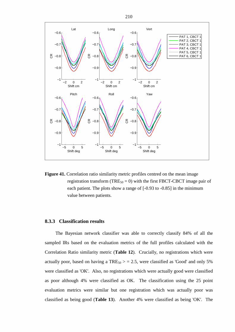
210

−5 0 5−1

−0.9

−0.8

−0.7

−0.6

Shift deg

CR

Pitch

−5 0 5−1

−0.9

−0.8

−0.7

−0.6

Shift deg

CR

Roll

−5 0 5−1

−0.9

−0.8

−0.7

−0.6

Shift deg

CR

Yaw

−2 0 2−1

−0.9

−0.8

−0.7

−0.6

Shift cm

CR

Lat

−2 0 2−1

−0.9

−0.8

−0.7

−0.6

Shift cmC

R

Long

−2 0 2−1

−0.9

−0.8

−0.7

−0.6

Shift cm

CR

Vert

PAT 1, CBCT 1PAT 2, CBCT 1PAT 3, CBCT 1PAT 4, CBCT 1PAT 5, CBCT 1PAT 6, CBCT 1

Figure 41. Correlation ratio similarity metric profiles centred on the mean image

registration transform (TRE50 = 0) with the first FBCT-CBCT image pair of

each patient. The plots show a range of [-0.93 to -0.85] in the minimum

value between patients.

8.3.3 Classification results

The Bayesian network classifier was able to correctly classify 84% of all the

sampled IRs based on the evaluation metrics of the full profiles calculated with the

Correlation Ratio similarity metric (Table 12). Crucially, no registrations which were

actually poor, based on having a TRE50 > = 2.5, were classified as 'Good' and only 5%

were classified as 'OK'. Also, no registrations which were actually good were classified

as poor although 4% were classified as OK. The classification using the 25 point

evaluation metrics were similar but one registration which was actually poor was

classified as being good (Table 13). Another 4% were classified as being 'OK'. The

211

classification results for the chamfer matching algorithm gave a similar level of

performance as those for the correlation ratio (Table 14 & Table 15).

−5 0 5−1

−0.9

−0.8

−0.7

−0.6

Shift deg

CR

Pitch

−5 0 5−1

−0.9

−0.8

−0.7

−0.6

Shift deg

CR

Roll

−5 0 5−1

−0.9

−0.8

−0.7

−0.6

Shift deg

CR

Yaw

−2 0 2−1

−0.9

−0.8

−0.7

−0.6

Shift cm

CR

Lat

−2 0 2−1

−0.9

−0.8

−0.7

−0.6

Shift cm

CR

Long

−2 0 2−1

−0.9

−0.8

−0.7

−0.6

Shift cmC

R

Vert

CBCT 1CBCT 2CBCT 3

Figure 42. Correlation ratio similarity metric profiles centred on the mean image

registration transform (TRE50 = 0) for the first three FBCT-CBCT image

pairs of patient 1. The plots show a range of [-0.9 to -0.83] in the minimum

value between patients.

212

Table 12. Confusion table showing classification of TRE50 values using a Bayesian network based on the similarity metric full profile evaluation metrics for image registrations performed using the correlation ratio.

Actual

Good

TRE50<=0.6 OK

0.6<TRE50<2.5 Poor

TRE50>=2.5

Good 143 (30) 25 (5%) 0 (0%)

OK 19 (4%) 118 (25%) 22 (5%) Classified As

Poor 0 (0%) 14 (3%) 138 (29%)

Table 13. Confusion table showing classification of TRE50 values using a Bayesian network based on the similarity metric 25 point evaluation metrics for image registrations performed using the correlation ratio.

Actual

Good

TRE50<=0.6 OK

0.6<TRE50<2.5 Poor

TRE50>=2.5

Good 134 (30) 20 (5%) 1 (0%)

OK 22 (4%) 108 (25%) 19 (4%) Classified As

Poor 0 (0%) 14 (3%) 129 (29%)

213

Table 14. Confusion table showing classification of TRE50 values using a Bayesian network based on the similarity metric full profile evaluation metrics for image registrations performed using the chamfer match.

Actual

Good

TRE50<=0.6 OK

0.6<TRE50<2.5 Poor

TRE50>=2.5

Good 129 (35%) 23 (6%) 0 (0%)

OK 40 (10%) 58 (15%) 9 (2%) Classified As

Poor 0 (0%) 37 (10%) 89 (23%)

Table 15. Confusion table showing classification of TRE50 values using a Bayesian network based on the similarity metric 25 point evaluation metrics for image registrations performed using the chamfer match.

Actual

Good

TRE50<=0.6 OK

0.6<TRE50<2.5 Poor

TRE50>=2.5

Good 111 (32) 15 (4%) 0 (0%)

OK 28 (8%) 51 (14%) 6 (2%) Classified As

Poor 6 (2%) 46 (13%) 89 (25%)

214

8.4 Discussion

In this chapter, the IR uncertainties were quantified using TRE50 for the two IR

algorithms based on Chamfer matching and Correlation Ratio. While the random error

was small for both algorithms there were a significant number of registrations with

TRE50 > 2.5mm. Similarity metric profiles centred on the IR rigid body transform

parameter output were calculated for a selection of the IRs. This demonstrated that no

single characteristic of the profiles, such as the minimum value, would have been

sufficient to classify the registrations as 'Good', 'OK' or 'Poor'. A preliminary study was

performed to determine if machine learning could classify the registrations based on the

inter-dependence of the 479, full profile SM evaluation metrics. The 84% correct

classification of the Bayesian network, with no classifications of 'Good' as 'Poor' or

'Poor' as good was very promising. The classification performance when SM evaluation

metrics were based on 25 points was similar to the performance with the six cardinal

axis profiles. This would enable a classification, based on 25 points, to be made at the

end of every IR without excessive additional computational time.

In practice classification methods such as the method presented here based on

calculating the Correlation Ratio at 25 points could be used by the operator to augment

the decision making process of whether an IR has been performed with sufficient level

of accuracy. The feedback would only be of benefit if it were to speed up the decision

making process. This would be the case if the operator chose to accept all the

registrations classified as 'Good' and only perform a cursory visual examination. If the

operator also chose to accept all those that were classified as 'OK' then 2% of these

would in fact be 'Poor'. As shown in this work such mis-registration results are in-

frequent. Furthermore, the operator is likely to detect a mis-registration if the TRE50

was much greater then 2.5mm and, in any fractionated radiotherapy treatment, the effect

of accepting a mis-registration with TRE50 just a little greater than 2.5mm would be

minimal if only a few fractions were affected. The 3% mis-classification of registrations

215

that are actually 'OK' but classified as 'Poor' is safe because the operator would be

prompted by the feedback to assess the registration more carefully.

This was a preliminary investigation to determine whether meaningful feedback on

the quality of an IR based on characteristics of the similarity metric could be achieved.

The results show great promise but there is potential for improvement. The evaluation

metrics may not be optimal to distinguish the difference between 'Good', 'OK' and 'Poor'

registrations. For instance the choice of 1mm, 0.5° for the calculation of DO_T, DO_R,

RON_T and RON_R. The spacing of the 25 point samples may also not have been

optimal. Points at ±1mm and ±2mm were chosen as these were similar to the TRE50

thresholds used to categorise the registrations as 'Good', 'OK' and 'Poor'. For instance,

sampling points at ±3mm might have improved classification of TRE50 near the 2.5mm

threshold.

The use of profiles only along the six cardinal axis of the parameter space would

have limited the accuracy with which the global minimum was located. Diagonal

profiles through the sample space might have improved the correlation of the ACC, DO

and RON based evaluation metrics with the TRE50 value and therefore the classification

performance. However, this would have been at the expense of increased computational

time.

Given the rate at which computer calculation speeds are increasing year on year,

concern over calculation time may be unfounded. However, determining the minimum

number of SM calculation points and their optimal locations without compromising

classification accuracy is an interesting question. Fast methods with fewer SM

calculation points are more likely to be implemented in clinical practice without the

need to upgrade computer hardware.

The BayesNet algorithm in the Weka software was chosen as it gave better results

than the other Bayesian based algorithms (NaiveBayes and NaiveBayesSimple) and

support vector machine algorithm (SMO). The default parameters for these algorithms

216

were used in each case and it is possible that optimisation of these parameters could

improve classification results. This is particularly the case for the support vector

machine algorithm where the width of the kernels has a large influence on performance.

Further work would be required to determine the optimum classifier for this dataset.

No attempt was made to determine the sensitivity of the machine learning

algorithm to the evaluation metrics. It is possible some of the evaluation metrics could

be left out without affecting the classification results. In addition no attempt was made

to determine the sensitivity of the machine learning algorithm to the thresholds of TRE50

chosen.

There was only a modest attempt to select equal number of 'Good', 'OK' and 'Poor'

registrations for the machine learning. However, the numbers of 'Good', 'OK' and 'Poor'

were fairly evenly distributed for the Correlation Ratio metric but weighted towards the

'Good' registrations for the Chamfer matching algorithm.

This study was limited by the inclusion of only 7 patients. More patients need to

be studied to determine if these results are robust and can be generalised to the entire

population.

The user feedback was performed for both the correlation ratio and chamfer match

similarity metrics. It may not be necessary to use exactly the same similarity metric as

that used in the original IR. The developers of IR algorithms often make compromises

in the calculation of the similarity metric in order to increase the speed of the algorithm

e.g. the number of random points chosen to calculate the joint histogram may have been

minimised. Performance of the classifier may increase if the number of randomly

sampled points were to be increased when calculating the SM for the SM evaluation

metrics.

The potential for user feedback on the quality of an IR was demonstrated for IR of

the skull. The same methods were used to classify the IRs of the prostate patients

however, the performance of the IR was variable between patients (Chapter 7, Figure

217

36), and there was a lack of a reasonable estimate of the ground truth by calculation of

the average of multiple registrations. This made the classification task impossible and

the results unsurprisingly were poor. It is clear that the automatic IR is more difficult

for the prostate than it is for the skull. This is probably due to the image content having

little contrast between the prostate and surrounding tissues and being plagued by image

blurring and artefacts due to patient motion, in particular the motion of air in the rectum.

Image acquisition for this site remains a challenge, as does the performance of the IR

algorithms. User feedback on the quality of a prostate IR would be of great benefit if it

could be made possible.

8.5 Conclusion

The similarity metric (SM) calculated for profiles along the cardinal axis of the

three translation and three rotation axis of the rigid body transform parameter space

were evaluated. None of the SM profile evaluation metrics (minimum value, accuracy,

risk of non convergence, distinctiveness of optimum), calculated with the correlation

ratio, were able to singularly predict the known target registration error (TRE50).

Supervised machine learning using a Bayesian Network with all the SM profile

evaluation metrics as inputs, was able to correctly classify 84% of all the sampled IRs

into three levels: 'Poor', 'OK' and 'Good'. No 'Poor' registrations were classified as

'Good' and no 'Good' registrations were classified as 'Poor'. Furthermore, a similar level

of classification performance was achieved based on similarity evaluation metrics

derived from the SM calculated at just 25 points in the vicinity of the transform returned

by the IR algorithm. This demonstrates that it is feasible to provide user feedback on

the quality of an IR. Such feedback could give confidence to the user that an IR is of

acceptable quality and remove the need for a visual check.

218

8.6 Future work

The methods described above show that it is feasible to use a machine learning

algorithm to create a classifier which determines the likelihood that an IR is of good

quality, in order to provide feedback to the user. Further optimisation of these methods

could improve the performance of the classifier. For instance, a number of questions

remain unanswered. Is the BayesNet algorithm the most appropriate? If so, do the

default parameters give the best results? What is the optimal number and location of

similarity metric calculation points?

Any future work would benefit from a larger sample of patient data to ensure the

methods are sufficiently generalised. In order to provide user feedback for IR in other

anatomical sites these methods would need to be adapted and optimised with supervised

learning based on appropriate training images for that site.

The lower and upper limits of 0.6mm and 2.5mm on the TRE50 IR quality metric,

which were determined from a simple single observer study, gave a good starting point

for this study, but may not be optimal. The performance of human observers in

performing IR and assessing IR quality is relatively unknown in image guided

radiotherapy. To fully determine the value of the methods devised in this study the

performance of a human observer study would be required to determine the acceptability

of an image registration for clinical use. Such a study would need to limit the time

available to the observer. This would allow comparison of the automatic user feedback

methods presented here with observer performance.

219

Chapter 9

Conclusions and future work

9.1 Conclusions

The aim of this thesis was to address the hypothesis that,

"the residual geometric uncertainties in the IGRT process,

introduced by the IGRT equipment, are sufficiently small that they do not

pose a risk of significant geometrical error in treatment delivery."

This was achieved by investigating the key causes of potential error of image

geometrical accuracy, image registration performance and automatic couch positioning

accuracy. Methods of measuring system performance including reproducibility and

accuracy were developed and new metrics devised where necessary. These were

employed to quantify the geometric uncertainties arising from the key components of

the IGRT system. In general, the geometric uncertainties measured were less than 1mm

and were therefore considerably less than the remaining geometrical uncertainties in

IGRT e.g. target volume delineation errors are typically greater than 2mm. However,

the uncertainties arising from image registration when the required anatomical structures

were not imaged with adequate quality to reproducibly and robustly perform image

registration were significantly greater than 1mm. Automatic image registration of the

prostate was found to be unreliable for many of the CBCT images investigated in this

study.

220

In the particular instance of IGRT for intra-cranial tumours the hypothesis can be

accepted. However, a larger than normal geometric error could arise from each of the

three identified components simultaneously and this should be considered. Given the

observed measurements in chapters 3, 5 and 6, the CBCT-MV isocentre error could be

as large as 0.8 mm, the couch positioning error could be 1mm and the image registration

error could be 2mm. In this instance the combined error would be 3.8mm which would

be a significant contribution to the overall error. However, it would be unlikely that such

an error is systematic throughout the course of treatment. But it does highlight the

importance of regular checks to ensure good geometrical calibration of the CBCT-MV

isocentre and the need to carefully identify and reduce any significant misalignments

after automatic image registration when performing radiotherapy with low numbers of

fractions.

In the case of IGRT for prostate radiotherapy then the geometric errors arising

from CBCT-MV isocentre and couch positioning are insignificant relative to the

remaining geometric uncertainties in the process. However, the image registration errors

are proportionately large and therefore the hypothesis cannot be accepted.

9.1.1 Chapter 3 - Quantification of misalignments in cone beam CT based

IGRT equipment

CBCT-MV isocentre alignment measurements, performed over a two year period,

were reviewed showing that alignment was accurate to 0.2 mm and reproducible with a

standard deviation of 0.3 mm. The maximum observed misalignment in any direction

was 0.5 mm. This demonstrates the Synergy® system imaging geometry is stable and

reproducible over time and there is no requirement to re-calibrate, by re-acquisition of

flex-maps, at frequencies greater than the manufacturers recommendation of once per

year. The consequence of these findings are:

• the system is suitable for performing stereotactic body radiation therapy as per

AAPM task group report 142 [8] with CBCT-MV alignment errors less than

1mm.

221

• the errors are sufficiently small that they do not contribute significantly to the

total margin, when combined in quadrature, with other known uncertainties in

treatment plan preparation and delivery with standard deviations of 1 mm or

greater.

The review of seven months 2D kV panel position measurements indicated that

the reproducibility of the measurement was not adequate to ensure alignment within

1mm. Investigation of outliers showed misalignments of 1.5mm were not predictive of

measurements of CBCT-MV alignment and image sharpness. The reliability of these

measurements was therefore questionable.

The additional research question,

"Can the methods of measuring geometric stability of a CBCT based

IGRT system using a commercially available phantom be improved and

automated to; (a) improve accuracy to ensure alignment between CBCT

image and MV beam is within 1mm and (b) improve efficiency of

measurement by integration of tests on one phantom?",

was also investigated. The methods for measuring CBCT-MV isocentre

alignment with the QUASAR™ Penta-Guide phantom were shown to be equivalent to

the previous method using a ball bearing and the software tool in the XVI Synergy®

software. Measurement of CBCT-MV isocentre alignment with the Penta-Guide

phantom has the potential to be implemented on any integrated kV-CBCT based IGRT

system making it manufacturer independent. Furthermore, a measurement of image

sharpness can also be performed using the CBCT images acquired of the Penta-Guide

phantom during the CBCT-MV alignment measurement. The combined CBCT-MV

alignment and image sharpness measurements could significantly reduce the time

required to perform these measurements as part of a programme of quality control

checks to ensure safe use of CBCT based IGRT systems.

222

The image sharpness measurement performed on the Penta-Guide phantom was

able to infer systematic misalignment of the kV tube and imaging panel, greater than

0.4mm, in a direction perpendicular to the rotation axis. Such misalignments would not

be detected by the CBCT-MV alignment test and could cause noticeable deterioration of

image quality.

9.1.2 Chapter 4 - Target Registration Error

In chapter 4, a novel method of calculating the target registration error is proposed

based on the mean displacement of points on the surface of a sphere with relevant

diameter. The method has some advantages over other methods previously reported,

such as the mean displacement of arbitrary points or the mean displacement of a grid of

points spanning the imaged field of view. Its design facilitates the interpretation and

analysis of image registration errors and the choice of sphere diameter which is centred

on the megavoltage isocentre increases its relevance to the clinical setting. The target

registration error was used to condense the six parameters of the rigid body transform

error into a single metric. This enabled the analysis of both couch position error in

chapter 5 and image registration errors in chapters 6 and 7 and was also used as a metric

of image quality for supervised training in chapter 8.

9.1.3 Chapter 5 - Measurement of automatic patient support movement

accuracy

A novel method for measuring the accuracy of relative couch movements on both

the Synergy® and Hexapod couch systems was developed and analysed using the

concept of TRE50 as described in Chapter 4. The typical median TRE50 couch position

errors were between 0.5 mm and 0.7 mm for the Hexapod system with maximum

223

measured TRE50 errors of 1.1mm. These errors are small in comparison with other

uncertainties in the radiotherapy process.

9.1.4 Chapters 6 and 7 - Measurement of automatic image registration

uncertainties for intra-cranial and prostate tumours.

In chapter 6 the accuracy, precision and robustness of image registration was

studied for intra-cranial tumours while in chapter 7 precision and robustness were

studied for image registration of the prostate. Techniques for performing such

measurements on commercial software without access to the source code of the

registration algorithm were developed.

In the case of intra-cranial tumours the accuracy assessed using the skull phantom

(Section 1.3.2) and defined in terms of TRE50 was significantly less than 0.5mm if the

CT slice width was less than or equal to 2.5mm. The precision (reproducibility), based

on patient images (Section 1.3.3), was such that the TRE50 was less than 1.3 mm for

90% of patients if the initial patient set-up errors were typical of those observed in

clinical practice i.e. < 3mm and 3°. There were also no registration failures. For intra-

cranial tumours, a random target registration error (TRE50) of up to 2.5 mm would be

considered reasonable. The risk of registration failure in this group is very low and a

visual check could be considered unnecessary. Note, a target registration error of

2.5mm, on the surface of a 50mm radius sphere, is equivalent to a 1 mm error in each of

three orthogonal directions combined with a 0.5° rotation. This should be a more than

adequate upper limit even for intracranial stereotactic radiotherapy treatments where

accuracy is paramount. However, a focussed visual check to catch target registration

errors noticeably greater than 2.5mm can be performed quickly and should not add

significantly to the overall decision to treat. It would therefore be prudent to maintain a

visual check as an additional safety measure.

224

For prostates the soft tissue image registration performance lacked robustness.

This made the measurement of precision difficult, except with images of a phantom or

for certain pairs of FBCT and CBCT patient images where prostate definition was

sufficient to enable image registration. For this reason a visual check of image

alignment is a definite requirement and there is a high likelihood that manual adjustment

will be required.

In both chapters 6 and 7 the additional research question,

"What is the relationship between image registration performance

and image quality and is there an optimum exposure setting which

minimises the radiation dose of imaging while maintaining adequate

performance of image registration for the image guidance task?",

was investigated. The imaging dose was reduced to determine the relationship

between imaging dose and image registration performance. For the prostate, the image

registration performance began to deteriorate rapidly for imaging doses less than 6 mGy.

However, since the automatic image registration performance was poor for patient

images it would seem that the appropriate practical imaging dose should be that required

by the users for manual image registration. For intra-cranial tumours the limit at which

image registration performance started to deteriorate rapidly (with decreasing image

dose) was not found even at extremely low doses of 8 µGy. There was a slight

deterioration for imaging doses less than 0.4 mGy. Since 8 µGy is extremely low in the

context of the dose received by the patient from radiotherapy it would seem unnecessary

to reduce the dose further. Hence, a dose of 0.4mGy could be considered as optimum.

This is a factor of ten lower than that which can be set under normal operation of the

clinical system.

225

9.1.5 Chapter 8 - Image registration quality likelihood metrics based on

similarity metric surface shape

In chapter 8, the feasibility of providing user feedback on the quality of the image

registration in order to provide confidence to the user that an image registration is of

acceptable quality for clinical use was investigated. The similarity metric (SM) was

calculated for profiles along the cardinal axis of the three translation and three rotation

axis of the rigid body transform parameter space. These SM profiles passed through and

were centred on the position returned by the image registration algorithm. In some cases

this was very close to the global maximum and in others further away. The target

registration error was used as a measure of the quality of the image registration. The

profiles were characterised by means of evaluation metrics such as the minimum value,

accuracy, distinctiveness of optimum and risk of non-convergence. Supervised machine

learning was used to train a classifier based on Bayesian Networks to distinguish the

quality of an image registration which utilised the evaluation metrics of the SM profiles.

The classifier was able to correctly classify 84% of all the sampled image registrations

into three levels: 'Poor', 'OK' and 'Good'. No 'Poor' registrations were classified as

'Good' and no 'Good' registrations were classified as 'Poor'. This demonstrates that it is

feasible to provide user feedback on the quality of an image registration. Such feedback

could give confidence to the user that an image registration is of acceptable quality and

remove the need for a visual check.

9.2 Future Work

The precision of image registration was found to be high (TRE50 < 0.5 mm) in the

head with the 'Elekta Correlation Ratio' algorithm but slightly less robust than with the

'Elekta Chamfer' algorithm. The 'Elekta Chamfer' algorithm which has the advantage of

being much faster to compute was less precise. Arguably, the application of the 'Elekta

Chamfer' algorithm alone is sufficient for most intra-cranial applications but for

226

stereotactic applications where greater accuracy is required application of the 'Elekta

Chamfer' algorithm first, followed by the 'Elekta Correlation Ratio' algorithm is likely to

be optimal. This would have the advantage of greater speed than using the 'Elekta

Correlation Ratio' algorithm alone because the 'Elekta Chamfer' algorithm would

provide a more optimal starting position for optimisation using the 'Elekta Correlation

Ratio' algorithm. It would also reduce the number of registration failures. This was not

tested in Chapter 6 but should the hypothesis be proven the method could be of clinical

benefit.

In the prostate, a clear dose relationship with image registration precision was

observed. This will help optimise the exposure settings in clinical practice to facilitate

automatic image registration. However it is clear from the image registrations on

patient images that reduced image quality due to patient motion during scanning and

deformation of the prostate is a problem for this clinical site. A repeat of this study

would be interesting to determine if, the controls implemented by radiographers to

ensure that rectal diameter is not large for the FBCT scan, and that dietary advice is

adhered to, has been effective. The reduction of FBCT slice width since the acquisition

of the images used in Chapter 7 may also improve the robustness of the image

registration of prostates. Given adequate image quality the performance of the

algorithm with changes to the size and shape of the mask would also be a line of future

investigation.

In 2009, a stereotactic technique for treating lung patients with hypo-fractionated

radiotherapy was implemented at SJIO. Since the dose per fraction is very large and

there are only 3-5 fractions it is critical that the dose is delivered to the correct place.

For this reason the technique is heavily dependent on cone beam CT imaging for

guidance. Until recently, the image registration has been performed manually but, with

the introduction of the region-of-interest based image registration of XVI v4.5,

automatic image registration is being considered. A study of the performance of the

image registration as performed in chapters 6 and 7 for the head and prostate could

227

reassure the operators (radiographers) that the algorithm is safe to use. Automatic

image registration has the potential to make the image matching process more efficient

and thereby reduce treatment times for these treatments. Furthermore, the introduction

of user feedback such as that developed in Chapter 8 would be of benefit in this

treatment site.

The lack of data on the inter- and intra-operator variability of image registration

for image guidance with CBCT images makes comparison between automatic and

manual methods impossible. There is also little data on the fundamental limits of an

observer to detect misalignments of images and how this might be affected by: the

visual representation of the registered images; how the operator interacts with the

images; and the quality of the image data. This also makes it impossible to know

whether an expert observer can reliably define an image registration as a gold standard

in order to bench mark automatic algorithms. The level of expertise of the operator is

also an unknown quality in the detection of image misalignment. While these studies

are difficult, the use of methods such as those by Fitzpatrick et al [132] would be

valuable research in an effort to improve the quality of IGRT. The VHMP phantom

used in chapters 5 and 7 would also be a useful tool for these studies. For instance, it

might not be safe practice to reduce imaging dose so low that an operator cannot reliably

validate visually the image registration, even if the automatic algorithm is highly robust

and very precise.

The classification of image registrations (Chapter 8), based on analysis of the

similarity metric over the parameter space in the vicinity of the optimum found by the

algorithm, warrants a more thorough investigation. The methods need further

optimisation e.g. choice of spacing for the 25 sample points, calculation of the SM

evaluation metrics and the choice of Bayesian networks as a machine learning

algorithm. Application of these methods to other clinical sites such as the lung and

spinal vertebrae would also have value.

228

Deformable image registration is becoming available in commercial products.

This will enable image registration of PET-CT and MR images to a planning FBCT to

improve the accuracy of target and organ at risk delineation. Deformable image

registration is also likely to be used in adaptive radiotherapy strategies and calculation

of cumulative dose distributions for dose response prediction. Automatic feedback from

the algorithm indicating areas of potential misalignment will be of immense value to aid

the operator in the process of validating individual image registrations.

For intra-cranial tumours the treatment errors after correction of patient position

based on CBCT image guidance are less than 1mm. Treatment beam errors such as

radiation dose accuracy, MLC leaf calibration and dose calculation errors are also of a

similar magnitude. This leaves the accuracy of the target delineation as the greatest

uncertainty in the radiotherapy process. Target delineation leads to systematic errors

which have greatest impact on the size of the margin required [21,22]. Accuracy of

target delineation is also the most difficult to quantify and is therefore less well

understood. With pre-IGRT margin sizes an under estimate in the delineation

uncertainty would have been partially compensated by the larger margin required to

encompass the greater uncertainties of patient set-up. With margins based on accurate

IGRT the probability of the target not being covered due to target delineation error will

be greater. For this reason margin reduction due to IGRT processes should be treated

with extreme caution and should be the subject of controlled clinical trials. It also

highlights the need for better understanding of target delineation errors. MRI and PET-

CT imaging modalities will play an important role here.

9.3 Impact and novel contributions

The work of Chapter 3 was published in Physics in Medicine and Biology in 2008

[71]. The CBCT-MV isocentre method was subsequently used in a national evaluation

of IGRT equipment which demonstrated its transferability to a CBCT based IGRT

system from another manufacturer [195].

229

The methods of the CBCT-MV alignment and image sharpness checks are being

further developed by a company that specialises in quality assurance software for

diagnostic and radiotherapy imaging applications. The software is currently undergoing

a phase of clinical validation before being introduced as a weekly check. With the

Penta-Guide phantom introduced into clinical practice for quality assurance, regions of

interest within the air and the acrylic body of the phantom will be monitored in order to

calculate the contrast to noise ratio. It is not certain at this time how useful this

information will be, but it has the potential to detect sudden changes and trends in the

performance of the X-ray generating system. The commercialisation of the methods

presented in Chapter 3 will help make them available to the radiotherapy medical

physics community. In addition, a programme of work to review the existing quality

assurance programme of tests performed daily, at Leeds, is underway. The existing tests

use custom built equipment and have been unchanged for many years. The IGRT

checks, also performed on a daily basis are performed using the Penta-Guide phantom.

There is potential to perform all the tests using just the Penta-Guide phantom. In doing

so, any redundancy in the tests will be removed thereby improving the efficiency of

performing daily quality assurance tests. It is hoped, ultimately, that this will increase

the number of fractions that can be delivered per day on an IGRT treatment system.

The work presented in chapter 6 investigating image registration uncertainties with

images of a head phantom and patient images of the head was reported in Physics in

Medicine and Biology in 2009 [196]. Subsequently, dual quaternions were used to

improve the analysis and interpretation of the image registration performance data. The

use of dual quaternions for rigid body error calculations is a unique contribution to the

analysis of image registration errors in image guided radiotherapy and could be

published in a suitable journal. It is also intended to disseminate the results of image

registration of the prostate performed in Chapter 7.

230

The feasibility study of chapter 8 which investigates a method for user feedback on

the quality of image registration to aid decision processes has great potential. This work

will form the basis of a journal article.

In appendix A.7 a procedure for converting between two systems for specifying

rigid body transforms was devised. It would be beneficial to other medical physicists

working with these systems to publish this, as a technical note perhaps, in one of the

medical physics journals.

231

References

[1] Jaffray DA, Drake DG, Moreau M, Martinez AA Wong JW. A radiographic and tomographic imaging system integrated into a medical linear accelerator for localization of bone and soft-tissue targets. International Journal of Radiation Oncology Biology Physics 1999;45:773-789.

[2] Moore CJ, Amer A, Marchant T, et al. Developments in and experience of kilovoltage X-ray cone beam image-guided radiotherapy. Br J Radiol 2006;79 Spec No 1:S66-78.

[3] McBain CA, Henry AM, Sykes J, et al. X-ray volumetric imaging in image-guided radiotherapy: the new standard in on-treatment imaging. Int J Radiat Oncol Biol Phys 2006;64:625-634.

[4] Sykes JR, Amer A, Czajka J Moore CJ. A feasibility study for image guided radiotherapy using low dose, high speed, cone beam X-ray volumetric imaging. Radiother Oncol 2005;77:45-52.

[5] Aird EGA. Second cancer risk, concomitant exposures and IRMER(2000). Br. J. Radiol. 2004;77:983-985.

[6] Harrison RM. Doses to organs and tissues from concomitant imaging in radiotherapy: a suggested framework for clinical justification. Br J Radiol 2008;81:970-974.

[7] HMSO. Ionising Radiation (Medical Exposure) Regulations 2000 Statutory Instrument 2000 No. 1059: HMSO, UK, 2000.

[8] Klein EE, Hanley J, Bayouth J, et al. AAPM Task Group 142 report: Quality assurance of medical accelerators. Medical Physics 2009;36:4197-4212.

[9] Bissonnette J-P. Quality assurance of image-guidance technologies. Semin Radiat Oncol 2007;17:278-286.

[10] Bissonnette J-P, Moseley DJ Jaffray DA. A quality assurance program for image quality of cone-beam CT guidance in radiation therapy. Medical Physics 2008;35:1807-1815.

[11] Delaney G, Jacob S, Featherstone C Barton M. The role of radiotherapy in cancer treatment. Cancer 2005;104:1129-1137.

[12] Bentzen SM, Heeren G, Cottier B, et al. Towards evidence-based guidelines for radiotherapy infrastructure and staffing needs in Europe: the ESTRO QUARTS project. Radiotherapy and Oncology 2005;75:355-365.

[13] National Radiotherapy Advisory Group NRAG, Radiotherapy: developing a world class service for England, 2007.

232

[14] Kuban D, Pollack A, Huang E, et al. Hazards of dose escalation in prostate cancer radiotherapy. International Journal of Radiation Oncology Biology Physics 2003;57:1260-1268.

[15] ICRU Report 62: Prescribing, Recording and Reporting Photon Beam Therapy (Supplement to ICRU Report 50), , 1999.

[16] Dearnaley DP, Sydes MR, Graham JD, et al. Escalated-dose versus standard-dose conformal radiotherapy in prostate cancer: first results from the MRC RT01 randomised controlled trial. The Lancet Oncology 2007;8:475-487.

[17] Jordan TJ Williams PC. The design and performance characteristics of a multileaf collimator. Physics in Medicine and Biology 1994;39:231.

[18] Thomas B. IMRT: a review and preview. Physics in Medicine and Biology 2006;51:R363.

[19] Otto K. Volumetric modulated arc therapy: IMRT in a single gantry arc. Medical Physics 2008;35:310-317.

[20] Guckenberger M, Richter A, Krieger T, Wilbert J, Baier K Flentje M. Is a single arc sufficient in volumetric-modulated arc therapy (VMAT) for complex-shaped target volumes? Radiotherapy and Oncology 2009;93:259-265.

[21] Bidmead M, Coffey M, Crellin A, Dobbs J, Driver D Greener A. Geometric uncertainties in radiotherapy: defining the target volume.: British Institute of Radiology, 2003.

[22] van Herk M, Remeijer P, Rasch C Lebesque JV. The probability of correct target dosage: dose-population histograms for deriving treatment margins in radiotherapy. International Journal of Radiation Oncology, Biology, Physics 2000;47:1121-1135.

[23] Uwe S et al. The calibration of CT Hounsfield units for radiotherapy treatment planning. Physics in Medicine and Biology 1996;41:111.

[24] Biederer J, Dinkel J, Remmert G, et al. 4D-Imaging of the Lung: Reproducibility of Lesion Size and Displacement on Helical CT, MRI, and Cone Beam CT in a Ventilated Ex Vivo System. International Journal of Radiation Oncology Biology Physics 2009;73:919-926.

[25] Rietzel E, Chen GT, Choi NC Willet CG. Four-dimensional image-based treatment planning: Target volume segmentation and dose calculation in the presence of respiratory motion. Int J Radiat Oncol Biol Phys 2005;61:1535-1550.

[26] Mancosu P, Bettinardi V, Passoni P, et al. Contrast enhanced 4D-CT imaging for target volume definition in pancreatic ductal adenocarcinoma. Radiotherapy and Oncology 2008;87:339-342.

[27] Dieleman EMT, Senan S, Vincent A, Lagerwaard FJ, Slotman BJ van Sörnsen de Koste JR. Four-dimensional computed tomographic analysis of esophageal

233

mobility during normal respiration. International Journal of Radiation Oncology Biology Physics 2007;67:775-780.

[28] Khoo VS, Dearnaley DP, Finnigan DJ, Padhani A, Tanner SF Leach MO. Magnetic resonance imaging (MRI): considerations and applications in radiotherapy treatment planning. Radiotherapy and Oncology 1997;42:1-15.

[29] Jarritt PH, Carson KJ, Hounsell AR Visvikis D. The role of PET/CT scanning in radiotherapy planning. Br J Radiol 2006;79:S27-35.

[30] Zaidi H, Vees H Wissmeyer M. Molecular PET/CT Imaging-Guided Radiation Therapy Treatment Planning. Academic Radiology 2009;16:1108-1133.

[31] Hugo GD, Yan D Liang J. Population and patient-specific target margins for 4D adaptive radiotherapy to account for intra- and inter-fraction variation in lung tumour position. Physics in Medicine and Biology 2007;52(1)(pp 257-274).

[32] McKenzie AL, van Herk M Mijnheer B. The width of margins in radiotherapy treatment plans. Physics in Medicine & Biology 2000;45:3331-3342.

[33] Hee Chul P, Jinsil S, Kwang Hyub H, Chae Yoon C, Young Myoung M Chang Ok S. Dose-response relationship in local radiotherapy for hepatocellular carcinoma. International journal of radiation oncology, biology, physics 2002;54:150-155.

[34] Mac Manus M, Hicks R, Matthews J, et al. Positron emission tomography is superior to computed tomography scanning for response-assessment after radical radiotherapy or chemoradiotherapy in patients with non-small-cell lung cancer. J Clin Oncol. 2003;21:1285-1292.

[35] Eschmann S, Paulsen F, Reimold M, et al. Prognostic impact of hypoxia imaging with 18F-misonidazole PET in non-small cell lung cancer and head and neck cancer before radiotherapy. J Nucl Med. 2005;46:253-260.

[36] Rockne R et al. Predicting the efficacy of radiotherapy in individual glioblastoma patients in vivo: a mathematical modeling approach. Physics in Medicine and Biology 2010;55:3271.

[37] Verellen D, De Ridder M Storme G. A (short) history of image-guided radiotherapy. Radiother Oncol 2008;86:4-13.

[38] Xing L, Thorndyke B, Schreibmann E, et al. Overview of image-guided radiation therapy. Medical Dosimetry 2006;31:91-112.

[39] Dawson LA Sharpe MB. Image-guided radiotherapy: rationale, benefits, and limitations. The Lancet Oncology 2006;7:848-858.

[40] Wu J, Haycocks T, Alasti H, et al. Positioning errors and prostate motion during conformal prostate radiotherapy using on-line isocentre set-up verification and implanted prostate markers. Radiotherapy and Oncology 2001;61:127-133.

234

[41] Feldkamp LA, Davis LC Kress JW. Practical Cone-Beam Algorithm. Journal of the Optical Society of America a-Optics Image Science and Vision 1984;1:612-619.

[42] Korreman S, Rasch C, McNair H, et al. The European Society of Therapeutic Radiology and Oncology-European Institute of Radiotherapy (ESTRO-EIR) report on 3D CT-based in-room image guidance systems: a practical and technical review and guide. Radiother Oncol 2010;94:129-144.

[43] Ruchala KJ, Olivera GH, Schloesser EA Mackie TR. Megavoltage CT on a tomotherapy system. Phys Med Biol 1999;44:2597-2621.

[44] Morin O, Gillis A, Chen J, et al. Megavoltage cone-beam CT: system description and clinical applications. Medical Dosimetry 2006;31:51-61.

[45] Uematsu M, Fukui T, Shioda A, et al. A dual computed tomography linear accelerator unit for stereotactic radiation therapy: A new approach without cranially fixated stereotactic frames. International Journal of Radiation Oncology Biology Physics 1996;35:587-592.

[46] Grills IS, Hugo G, Kestin LL, et al. Image-Guided Radiotherapy via Daily Online Cone-Beam CT Substantially Reduces Margin Requirements for Stereotactic Lung Radiotherapy. International Journal of Radiation Oncology Biology Physics 2008;70:1045-1056.

[47] Pisani L, Lockman D, Jaffray D, Yan D, Martinez A Wong J. Setup error in radiotherapy: on-line correction using electronic kilovoltage and megavoltage radiographs. International Journal of Radiation Oncology Biology Physics 2000;47:825-839.

[48] de Boer HC Heijmen BJ. A protocol for the reduction of systematic patient setup errors with minimal portal imaging workload. Int J Radiat Oncol Biol Phys 2001;50:1350-1365.

[49] Bel A, van Herk M, Bartelink H Lebesque JV. A verification procedure to improve patient set-up accuracy using portal images. Radiother Oncol 1993;29:253-260.

[50] Ellis RE, Peters TM, Craig T, et al. Comparison of Correction Protocols for Image-Guided Radiation Therapy Medical Image Computing and Computer-Assisted Intervention - MICCAI 2003, vol. 2879: Springer Berlin / Heidelberg, 2003; 264-270.

[51] Redpath AT, Wright P Muren LP. The contribution of on-line correction for rotational organ motion in image-guided radiotherapy of the bladder and prostate. Acta Oncol 2008;47:1367-1372.

[52] Guckenberger M, Meyer J, Wilbert J, Baier K, Sauer O Flentje M. Precision of image-guided radiotherapy (IGRT) in six degrees of freedom and limitations in clinical practice. Strahlenther Onkol 2007;183:307-313.

[53] Rijkhorst E-J, van Herk M, Lebesque JV Sonke J-J. Strategy for Online Correction of Rotational Organ Motion for Intensity-Modulated Radiotherapy of

235

Prostate Cancer. International Journal of Radiation Oncology Biology Physics 2007;69:1608-1617.

[54] Yan D. Adaptive Radiotherapy: Merging Principle Into Clinical Practice. Semin Radiat Oncol 2010;20:79-83.

[55] Group AIEE, A Road Map for Research, Development and Assessment of Image Guided Radiotherapy (IGRT) During its Implementation in the UK. ACORRN, 2008.

[56] Lillicrap SC, Higson GR O'Connor AJ. Radiotherapy equipment standards from the International Electrotechnical Commission. Br J Radiol 1998;71:1225-1228.

[57] Letourneau D, Wong JW, Oldham M, et al. Cone-beam-CT guided radiation therapy: technical implementation. Radiotherapy & Oncology 2005;75:279-286.

[58] Sorcini B Tilikidis A. Clinical application of image-guided radiotherapy, IGRT (on the Varian OBI platform). Cancer/Radiothérapie 2006;10:252-257.

[59] Yoo S, Kim GY, Hammoud R, et al. A quality assurance program for the on-board imager. Medical Physics 2006;33:4431-4447.

[60] Lehmann J, Perks J, Semon S, Harse R Purdy JA. Commissioning experience with cone-beam computed tomography for image-guided radiation therapy. Journal of Applied Clinical Medical Physics 2007;8:2354.

[61] Sharpe MB, Moseley DJ, Purdie TG, Islam M, Siewerdsen JH Jaffray DA. The stability of mechanical calibration for a kV cone beam computed tomography system integrated with linear accelerator. Medical Physics 2006;33:136-144.

[62] Fox T, Huntzinger C, Johnstone P, Ogunleye T Elder E. Performance evaluation of an automated image registration algorithm using an integrated kilovoltage imaging and guidance system. J Appl Clin Med Phys 2006;7:97-104.

[63] Cho Y, Moseley DJ, Siewerdsen JH, et al. Accurate technique for complete geometric calibration of cone-beam computed tomography systems. Medical Physics 2005;32:968-983.

[64] Gayou O Miften M. Commissioning and clinical implementation of a mega-voltage cone beam CT system for treatment localization. Med Phys 2007;34:3183-3192.

[65] Mao W, Lee L, Xing L, Mao W, Lee L Xing L. Development of a QA phantom and automated analysis tool for geometric quality assurance of on-board MV and kV x-ray imaging systems. Medical Physics 2008;35:1497-1506.

[66] Lutz W, Winston KR Maleki N. A system for stereotactic radiosurgery with a linear accelerator. International Journal of Radiation Oncology Biology Physics 1988;14:373-381.

[67] Amer A, Sykes J Moore C. Imaging panel skew correction and auto-focusing in radiotherapy cone beam imaging. Information Visualisation, 2004. IV 2004. Proceedings. Eighth International Conference on. 200492-97.

236

[68] ACR Technical Standard for Medical Physics Performance Monitoring of Image-Guided External Beam Radiation Therapy (IGRT). American College of Radiology, 2009.

[69] Marguet M Bodez V. Quality control of a kV cone beam computed tomography imaging system. [French]. Cancer/Radiotherapie 2009;13 (5):345-352.

[70] Saw CB, Yang Y, Li F, et al. Performance Characteristics and Quality Assurance Aspects of Kilovoltage Cone-Beam CT on Medical Linear Accelerator. Medical Dosimetry 2007;32:80-85.

[71] Sykes JR, Lindsay R, Dean CJ, Brettle DS, Magee DR Thwaites DI. Measurement of cone beam CT coincidence with megavoltage isocentre and image sharpness using the QUASAR Penta-Guide phantom. Phys Med Biol 2008;53:5275-5293.

[72] Langen KM, Meeks SL Pouliot J. Quality Assurance of Onboard Megavoltage Computed Tomography Imaging and Target Localization Systems for On- and Off-Line Image-Guided Radiotherapy. International Journal of Radiation Oncology Biology Physics 2008;71:S62-S65.

[73] Vogele M. An automatic therapy couch with 6 degrees of freedom based on a 3D sensor system first pre-clinical results. Industrial Informatics, 2004. INDIN '04. 2004 2nd IEEE International Conference on. 2004425-426.

[74] Meyer J, Wilbert J, Baier K, et al. Positioning accuracy of cone-beam computed tomography in combination with a HexaPOD robot treatment table. International Journal of Radiation Oncology, Biology, Physics 2007;67:1220-1228.

[75] Takakura T, Mizowaki T, Nakata M, et al. The geometric accuracy of frameless stereotactic radiosurgery using a 6D robotic couch system. Phys Med Biol 2010;55:1-10.

[76] Shepard SJ, Lin PP, Boone JM, et al., Quality Control in Diagnostic Radiology, AAPM Report No. 74, 2002.

[77] IPEM, Recommended Standards for the Routine Performance Testing of Diagnostic X-Ray Imaging Systems, Report 91, 2005.

[78] Letourneau D, Keller H, Sharpe MB Jaffray DA. Integral test phantom for dosimetric quality assurance of image guided and intensity modulated stereotactic radiotherapy. Medical Physics 2007;34:1842-1849.

[79] Letourneau D, Wong R Moseley D. Online planning and delivery technique for radiotherapy of spinal metastases using cone-beam CT: image quality and system performance. Int J Radiat Oncol Biol Phys 2007;67:1229 - 1237.

[80] Hill DL, Batchelor PG, Holden M Hawkes DJ. Medical image registration. Phys Med Biol 2001;46:R1-45.

[81] Kessler ML. Image registration and data fusion in radiation therapy. Br. J. Radiol. 2006;79:S99-S108.

237

[82] Huisman HJ, Futterer JJ, van Lin EN, et al. Prostate cancer: precision of integrating functional MR imaging with radiation therapy treatment by using fiducial gold markers. Radiology 2005;236:311-317.

[83] Luu QT, Levy RP, Miller DW, et al. A clinical interactive technique for MR-CT image registration for target delineation of intracranial tumors. Technol Cancer Res Treat 2005;4:275-281.

[84] Rosenman JG, P. ME, Tracton G Cullip TJ. Image Registration: An Essential Part of Radiation Therapy Treatment Planning. International Journal of Radiation Oncology Biology Physics 1998;40:197-205.

[85] Hristov DH Fallone BG. A grey-level image alignment algorithm for registration of portal images and digitally reconstructed radiographs. Medical Physics 1996;23:75-84.

[86] Khamene A, Bloch P, Wein W, Svatos M Sauer F. Automatic registration of portal images and volumetric CT for patient positioning in radiation therapy. Medical Image Analysis 2006;10:96-112.

[87] Leszczynski KW, Loose S Boyko S. An image registration scheme applied to verification of radiation therapy. Br J Radiol 1998;71:413-426.

[88] Smitsmans MH, de Bois J, Sonke JJ, et al. Automatic prostate localization on cone-beam CT scans for high precision image-guided radiotherapy. Int J Radiat Oncol Biol Phys 2005;63:975-984.

[89] Gao S, Zhang L, Wang H, et al. A deformable image registration method to handle distended rectums in prostate cancer radiotherapy. Medical Physics 2006;33:3304-3312.

[90] Malsch U, Thieke C Bendl R. Fast elastic registration for adaptive radiotherapy. Medical Image Computing & Computer-Assisted Intervention: MICCAI 2006;9:612-619.

[91] Malsch U, Thieke C, Huber PE Bendl R. An enhanced block matching algorithm for fast elastic registration in adaptive radiotherapy. Physics in Medicine & Biology 2006;51:4789-4806.

[92] Grau C, Muren LP, HÃ¸yer M, Lindegaard J Overgaard J. Image-guided adaptive radiotherapy - integration of biology and technology to improve clinical outcome. Acta Oncologica 2008;47:1182 - 1185.

[93] Larocque MP, Syme A, Allalunis-Turner J Fallone BG. ADC response to radiation therapy correlates with induced changes in radiosensitivity. Medical Physics 2010;37:3855-3861.

[94] Mathew L, Gaede S, Wheatley A, Etemad-Rezai R, Rodrigues GB Parraga G. Detection of longitudinal lung structural and functional changes after diagnosis of radiation-induced lung injury using hyperpolarized [sup 3]He magnetic resonance imaging. Medical Physics 2010;37:22-31.

238

[95] Xing L, Siebers J Keall P. Computational Challenges for Image-Guided Radiation Therapy: Framework and Current Research. Semin Radiat Oncol 2007;17:245-257.

[96] Sharpe M Brock. Kristy K. Quality Assurance of Serial 3D Image Registration, Fusion, and Segmentation. International journal of radiation oncology, biology, physics 2008;71:S33-S37.

[97] Fitzpatrick JM, Hill DL Maurer CR. Image registration in: Medical Image Processing and Analysis, vol. 2. Bellingham, WA, 2000: SPIE, 2000.

[98] Brown LG. A survey of image registration techniques. ACM Comput. Surv. 1992;24:325-376.

[99] Maintz JB Viergever MA. A survey of medical image registration. Med Image Anal 1998;2:1-36.

[100] Pluim JP, Maintz JB Viergever MA. Mutual-information-based registration of medical images: a survey. IEEE Trans Med Imaging 2003;22:986-1004.

[101] Zitova B Flusser J. Image registration methods: a survey. Image and Vision Computing 2003;21:977-1000.

[102] Insight into Images: Principles and Practice for Segmentation, Registration and Analysis, 2004.

[103] Yoo TS. Insight into Images “Principles and Practice for Segmentation, Registration, and Image Analysis” Peters, A K, Limited, 2004.

[104] Handbook of Medical Image Processing and Analysis (Second Edition) 2008.

[105] Klein S, Staring M Pluim JPW. Evaluation of Optimization Methods for Nonrigid Medical Image Registration Using Mutual Information and B-Splines. Image Processing, IEEE Transactions on 2007;16:2879-2890.

[106] Klein S. Optimisation Methods for Medical Image Registration Image Sciences Institute, University Medical Center Utrecht, vol. PhD. Utrecht: Utrecht, 2008.

[107] Glasbey CA van der Heijden GWAM. Alignment and sub-pixel interpolation of images using Fourier methods. Journal of Applied Statistics 2007;34:217-230.

[108] Brown M Lowe DG. Recognising Panoramas. International Conference on Computer Vision. Nice, France. 2003

[109] Feldmar J Ayache N. Rigid, affine and locally affine registration of free-form surfaces. Int. J. Comput. Vision 1996;18:99-119.

[110] Borgefors G. Hierarchical Chamfer Matching: A Parametric Edge Matching Algorithm. IEEE Trans. Pattern Anal. Mach. Intell. 1988;10:849-865.

[111] van Herk M Kooy HM. Automatic three-dimensional correlation of CT-CT, CT-MRI, and CT-SPECT using chamfer matching. Med Phys 1994;21:1163-1178.

239

[112] Roche A, Malandain G, Pennec X Ayache N, Multimodal Image Registration by Maximization of the Correlation Ratio. INRIA, 1998.

[113] Roche A, Malandain G, Pennec X Ayache N. The Correlation Ratio as a New Similarity Measure for Multimodal Image Registration Medical Image Computing and Computer-Assisted Interventation — MICCAI’98, vol. 1496/1998: Springer Berlin / Heidelberg, 1998; 1115.

[114] Lemieux L, Wieshmann UC, Moran NF, Fish DR Shorvon SD. The detection and significance of subtle changes in mixed-signal brain lesions by serial MRI scan matching and spatial normalization. Medical Image Analysis 1998;2:227-242.

[115] Viola P. Alignment by Maximization of Mutual Information Artificial Intelligence Laboratory, Massachusetts Institute of Technology, vol. PhD, 1995.

[116] Viola P Wells WM, 3rd. Alignment by Maximization of Mutual Information. International Journal of Computer Vision 1997;24:137–154.

[117] Wells WM, 3rd, Viola P, Atsumi H, Nakajima S Kikinis R. Multi-modal volume registration by maximization of mutual information. Med Image Anal 1996;1:35-51.

[118] Jannin P, Fitzpatrick JM, Hawkes DJ, Pennec X, Shahidi R Vannier MW. Validation of medical image processing in image-guided therapy. IEEE Trans Med Imaging 2002;21:1445-1449.

[119] West J, Fitzpatrick JM, Wang MY, et al. Comparison and evaluation of retrospective intermodality brain image registration techniques. J Comput Assist Tomogr 1997;21:554-566.

[120] Brock KK. Results of a Multi-Institution Deformable Registration Accuracy Study (MIDRAS). International Journal of Radiation Oncology Biology Physics 2010;76:583-596.

[121] van Herk M, de Munck JC, Lebesque JV, Muller S, Rasch C Touw A. Automatic registration of pelvic computed tomography data and magnetic resonance scans including a full circle method for quantitative accuracy evaluation. Med Phys 1998;25:2054-2067.

[122] Bender ET Tome WA. The utilization of consistency metrics for error analysis in deformable image registration. Physics in Medicine and Biology 2009;54:5561.

[123] Ceylan C, van der Heide UA, Bol GH, Lagendijk JJW Kotte ANTJ. Assessment of rigid multi-modality image registration consistency using the multiple sub-volume registration (MSR) method. Physics in Medicine & Biology 2005;50:N101-108.

[124] Dean CJ, Sykes JR, Cooper RA, et al. An evaluation of four CT-MRI co-registration techniques for radiotherapy treatment planning of prone rectal cancer patients. Accepted by British Journal of Radiology July 2010 2010.

240

[125] Barboriak DP Provenzale JM. Evaluation of software for registration of contrast-enhanced brain MR images in patients with glioblastoma multiforme. AJR Am J Roentgenol 2002;179:245-250.

[126] Sarkar A, Santiago RJ, Smith R Kassaee A. Comparison of manual vs. automated multimodality (CT-MRI) image registration for brain tumors. Med Dosim 2005;30:20-24.

[127] Li G, Xie H, Ning H, et al. A novel 3D volumetric voxel registration technique for volume-view-guided image registration of multiple imaging modalities. Int J Radiat Oncol Biol Phys 2005;63:261-273.

[128] Li G, Xie H, Ning H, et al. Accuracy of 3D volumetric image registration based on CT, MR and PET/CT phantom experiments. J Appl Clin Med Phys 2008;9:2781.

[129] Wong JC, Studholme C, Hawkes DJ Maisey MN. Evaluation of the limits of visual detection of image misregistration in a brain fluorine-18 fluorodeoxyglucose PET-MRI study. Eur J Nucl Med 1997;24:642-650.

[130] Phillips BL, Jiroutek MR, Tracton G, Elfervig M, Muller KE Chaney EL. Thresholds for human detection of patient setup errors in digitally reconstructed portal images of prostate fields. International Journal of Radiation Oncology Biology Physics 2002;54:270-277.

[131] Holton Tainter KS, Taneja U Robb RA. Quantitative validation of 3D image registration techniques. Medical Imaging 1995: Image Processing. 1 ed. San Diego, CA, USA. SPIE. 1995;2434:504-519.

[132] Fitzpatrick JM, Hill DL, Shyr Y, West J, Studholme C Maurer CR, Jr. Visual assessment of the accuracy of retrospective registration of MR and CT images of the brain. IEEE Trans Med Imaging 1998;17:571-585.

[133] Rodriguez-Carranza CE Loew MH. Design and evaluation of an automatic procedure for detection of large misregistration of medical images. IEEE Trans Med Imaging 2003;22:1445-1457.

[134] Kybic J Smutek D. Image registration accuracy estimation without ground truth using bootstrap Computer Vision Approaches to Medical Image Analysis, vol. 4241. Berlin: Springer-Verlag Berlin, 2006; 61-72.

[135] Kagawa K, Lee WR, Schultheiss TE, Hunt MA, Shaer AH Hanks GE. Initial clinical assessment of CT-MRI image fusion software in localization of the prostate for 3D conformal radiation therapy. International Journal of Radiation Oncology Biology Physics 1997;38:319-325.

[136] Lavely WC, Scarfone C, Cevikalp H, et al. Phantom validation of coregistration of PET and CT for image-guided radiotherapy. Medical Physics 2004;31:1083-1092.

[137] Moore CS, Liney GP Beavis AW. Quality assurance of registration of CT and MRI data sets for treatment planning of radiotherapy for head and neck cancers. J Appl Clin Med Phys 2004;5:25-35.

241

[138] Mutic S, Dempsey JF, Bosch WR, et al. Multimodality image registration quality assurance for conformal three-dimensional treatment planning. Int J Radiat Oncol Biol Phys 2001;51:255-260.

[139] Robar JL, Clark BG, Schella JW Kim CS. Analysis of patient repositioning accuracy in precision radiation therapy using automated image fusion. J Appl Clin Med Phys 2005;6:71-83.

[140] Yu CPD, Apuzzo MLJMD, Zee C-SMD Petrovich ZMD. A Phantom Study of the Geometric Accuracy of Computed Tomographic and Magnetic Resonance Imaging Stereotactic Localization with the Leksell Stereotactic System. Neurosurgery 2001;48:1092-1099.

[141] Zhang Y, Chu JCH, Hsi W, et al. Evaluation of Four Volume-Based Image Registration Algorithms. Medical Dosimetry 2009;34:317-322.

[142] Ardekani BA, Bachman AH Helpern JA. A quantitative comparison of motion detection algorithms in fMRI. Magnetic Resonance Imaging 2001;19:959-963.

[143] Isambert A, Bonniaud G, Lavielle F, Malandain G Lefkopoulos D. A phantom study of the accuracy of CT, MR and PET image registrations with a block matching-based algorithm. Cancer/Radiothérapie 2008;12:800-808.

[144] Smitsmans MHP, Wolthaus JWH, Artignan X, et al. Automatic localization of the prostate for on-line or off-line image-guided radiotherapy. International Journal of Radiation Oncology Biology Physics 2004;60:623-635.

[145] Wang H, Feng D Huang S-C. A statistical method for the assessment of 3-D medical image registration. Selected papers from the Pan-Sydney workshop on Visualisation - Volume 2. Sydney, Australia. Australian Computer Society, Inc. 2001;2:101-103.

[146] Skerl D, Tomazevic D, Likar B Pernus F. Evaluation of similarity measures for reconstruction-based registration in image-guided radiotherapy and surgery. International Journal of Radiation Oncology, Biology, Physics 2006;65:943-953.

[147] Dandekar O, Siddiqui K, Walimbe V Shekhar R. Image registration accuracy with low-dose CT: How low can we go? 2006 3rd Ieee International Symposium on Biomedical Imaging: Macro to Nano, Vols 1-3. New York: Ieee, 2006; 502-505.

[148] Pappas IPI, Styner M, Malik P, Remonda L Caversaccio M. Automatic method to assess local CT-MR Imaging registration accuracy on images of the head. American Journal of Neuroradiology 2005;26:137-144.

[149] Low DA Dempsey JF. Evaluation of the gamma dose distribution comparison method. Med Phys 2003;30:2455-2464.

[150] Hub M, Kessler M Karger C. Automatic Evaluation Of The Local Uncertainty Of Displacement Vector Fields Resulting From A B-Spline Deformable Registration Algorithm. ESTRO 2008 2008;88:S153.

242

[151] Bongartz G, Golding SJ, Jurik AG, et al., European Guildelines on Quality Criteria for Computed Tomography, 1994.

[152] Rossman K. Point spread-function, line spread function and modulation transfer function. Radiology 1969;93:252-272.

[153] Boone JM Seibert JA. An analytical edge spread function model for computer fitting and subsequent calculation of the LSF and MTF. Medical Physics 1994;21:1541-1545.

[154] White DR, Speller RD Taylor PM. Evaluating performance characteristics in computerized tomography. Br J Radiol 1981;54:221-231.

[155] The Phantom Laboratory. Catphan ® 500 and 600 Manual, 2004.

[156] Droege RT Morin RL. A practical method to measure the MTF of CT scanners. Medical Physics 1982;9:758-760.

[157] Droege RT Rzeszotarski MS. An MTF method immune to aliasing. Medical Physics 1985;12:721-725.

[158] Rajapakshe R, Luchka K Shalev S. A quality control test for electronic portal imaging devices. Medical Physics 1996;23:1237-1244.

[159] Hassan W. Calculation of the modulation transfer function from the square wave response function data with an interactive curve fitting software. Physica Medica 2002;18:25-31.

[160] Ichikawa K, Fujita H Sawada T. Novel MTF measurement method for medical image viewers using a bar pattern image. In: Galloway RL, ed. Medical Imaging 2003: Visualization, Image-Guided Procedures, and Display, vol. 5029. Bellingham: Spie-Int Society Optical Engineering, 2003; 624-631.

[161] Berbeco RI, Jiang SB, Sharp GC, Chen GT, Mostafavi H Shirato H. Integrated radiotherapy imaging system (IRIS): design considerations of tumour tracking with linac gantry-mounted diagnostic x-ray systems with flat-panel detectors. Phys Med Biol 2004;49:243-255.

[162] Kavan L, Collins S, Zara J O'Sullivan C. Skinning with Dual Quaternions. I3d 2007: Acm Siggraph Symposium on Interactive 3d Graphics and Games, Proceedings 2007:39-46.

[163] Kavan L, Collins S, Zara J O'Sullivan C. Geometric Skinning with Approximate Dual Quaternion Blending. Acm Transactions on Graphics 2008;27.

[164] Daniilidis K. Hand-eye calibration using dual quaternions. International Journal of Robotics Research 1999;18:286-298.

[165] Schmidt J, Vogt F Niemann H. Robust hand-eye calibration of an endoscopic surgery robot using dual quaternions. Pattern Recognition, Proceedings 2003;2781:548-556.

243

[166] Humphreys FJ, Bate PS Hurley PJ. Orientation averaging of electron backscattered diffraction data. Journal of Microscopy 2001;201:50-58.

[167] Humbert M, Gey N, Muller J Esling C. Determination of a Mean Orientation from a Cloud of Orientations. Application to Electron Back-Scattering Pattern Measurements. Journal of Applied Crystallography 1996;29:662-666.

[168] Krieger Lassen NC, Juul Jensen D Conradsen K. On the statistical analysis of orientation data. Acta Crystallographica Section A 1994;50:741-748.

[169] Gramkow C. On Averaging Rotations. Int. J. Comput. Vision 2001;42:7-16.

[170] Dekker N, Ploeger LS Van Herk M. Evaluation of cost functions for gray value matching of two-dimensional images in radiotherapy. Medical Physics 2003;30:778-784.

[171] Skerl D, Likar B Pernus F. A protocol for evaluation of similarity measures for rigid registration. IEEE Transactions on Medical Imaging 2006;25:779-791.

[172] Russell SJ Norvig P. Artificial Intelligence: A Modern Approach: Prentice Hall, 2003.

[173] Cooper GF Herskovits E. A Bayesian Method for the Induction of Probabilistic Networks from Data. Mach. Learn. 1992;9:309-347.

[174] Bouckaert RR. Bayesian Network Classifiers in Weka 2006. http://www.cs.waikato.ac.nz/~remco/weka.bn.pdf

[175] Burnside ES. Bayesian networks: Computer-assisted diagnosis support in radiology1. Academic Radiology 2005;12:422-430.

[176] Jayasurya K, Fung G, Yu S, et al. Comparison of Bayesian network and support vector machine models for two-year survival prediction in lung cancer patients treated with radiotherapy. Medical Physics 2010;37:1401-1407.

[177] Zhang HH, D'Souza WD, Shi L Meyer RR. Modeling Plan-Related Clinical Complications Using Machine Learning Tools in a Multiplan IMRT Framework. International Journal of Radiation Oncology Biology Physics 2009;74:1617-1626.

[178] El Naqa I. TU-D-204C-04: Machine Learning as New Tool for Predicting Radiotherapy Response. 6 ed. AAPM. 2010;37:3396-3396.

[179] Shiva KD, Shifeng C, Joseph OD, Sumin Z, Fang-Fang Y Lawrence BM. Decision Fusion of Machine Learning Models to Predict Radiotherapy-Induced Lung Pneumonitis Proceedings of the 2008 Seventh International Conference on Machine Learning and Applications: IEEE Computer Society, 2008.

[180] Tong L et al. Markerless gating for lung cancer radiotherapy based on machine learning techniques. Physics in Medicine and Biology 2009;54:1555.

[181] Marchant T, Synergy Quality Control and Troubleshooting. Email to: Sykes JR, 2005

244

[182] Canny J. A computational approach to edge detection. IEEE Transactions on Pattern Analysis and Machine Intelligence 1986;8:679-698.

[183] Hough P. A Method and Means for Recongnizing Complex Patterns. In: Patent U, ed., ed. G01T 5/00 (20060101); G01T 5/02 (20060101); G06K 9/46 (20060101), 1962.

[184] Sonka M Fitzpatrick JM. Handbook of Medical Imaging, vol. 2: Medical Image Processing and Analysis: SPIE Press, 2000.

[185] Lagarias JC, Reeds JA, Wright MH Wright PE. Convergence properties of the Nelder-Mead simplex method in low dimensions. SIAM J. Optim. 1999;9:112--147 (electronic).

[186] Schwarzband G Kiryati N. The point spread function of spiral CT. Phys Med Biol 2005;50:5307-5322.

[187] West JB, Fitzpatrick JM, Toms SA, Maurer CR Maciunas RJ. Fiducial point placement and the accuracy of point-based, rigid body registration. Neurosurgery 2001;48:810-816.

[188] Moler CB. Numerical Computing with MATLAB: Society for Industrial and Applied Maths, 2004.

[189] Shrimpton PC, Jessen KA, Geleijns J, Panzer W Tosi G. Reference doses in computed tomography. Radiation Protection Dosimetry 1998;80:55-59.

[190] van Herk M, Gilhuijs KG, de Munck J Touw A. Effect of image artifacts, organ motion, and poor segmentation on the reliability and accuracy of three-dimensional chamfer matching. Computer Aided Surgery 1997;2:346-355.

[191] van Herk M, RE: Image Registration research. Email to: Sykes JR, 24/09/2010

[192] Stroom JC, Koper PCM, Korevaaar GA, et al. Internal organ motion in prostate cancer patients treated in prone and supine treatment position. Radiotherapy and Oncology 1999;51:237-248.

[193] Seber GAF. Multivariate Observations: Wiley, 1984.

[194] Graham SA, Moseley DJ, Siewerdsen JH Jaffray DA. Compensators for dose and scatter management in cone-beam computed tomography. Medical Physics 2007;34:2691-2703.

[195] Sykes JR, Lindsay R, Stanley S, et al., Centre for Evidence Based Purchasing Evaluation Report: X-ray Tomographic Image Guided Radiotherapy Systems, 2010.

[196] Sykes JR, Brettle DS, Magee DR Thwaites DI. Investigation of uncertainties in image registration of cone beam CT to CT on an image-guided radiotherapy system. Phys Med Biol 2009;54:7263-7283.

[197] Weisstein EW. "Euler Angles." From MathWorld-A Wolfram Web Resource. http://mathworld.wolfram.com/EulerAngles.html

245

[198] Baker M. Maths-Dual Quaternions. http://www.euclideanspace.com/maths/algebra/realNormedAlgebra/other/dualQuaternion/index.htm

[199] Kavan L, Collins S, Zara J O'Sullivan C, Dual quaternions for rigid body transformation blending. Technical report TCD-CS-2006-46. Trinity College Dublin, 2006.

[200] Arun KS, Huang TS Blostein SD. Least-Squares Fitting of 2 3-D Point Sets. IEEE Transactions on Pattern Analysis and Machine Intelligence 1987;9:699-700.

Appendix A

Rigid body transformations: notation and

conversion

A.1 Introduction

In chapters 5, 6 and 7 errors between known and measured rigid body transform

parameters are calculated. The measured transform parameters are based on the IEC

1217 coordinate scheme where the angles are presented as Euler angles [197]. The

known or applied transform parameters use the coordinate scheme of the

VersorRigid3DTransform class of the ITK 3.12 software. These are the parameters

chosen to transform either the CT reference image set (Chapter 5) or CBCT image

(Chapter 6,7). A third notation for representing rigid body transformations called a Dual

Quaternion is also used in these chapters for the purpose of calculating the image

registration errors. The coordinate systems and notation are described in sections A.2,

A.3 & A.4. The theory of calculating the mean using dual quaternions is presented in

section A.5 and the transform error in section A.6.

Conversion between the Synergy® system's rigid body transform parameters and

that of the ITK VersorRigid3DTransform class is performed extensively in chapters 4

and 5. Section A.7 reports on the investigations required to establish the

correspondence between the two sets of parameters and the method of converting

between them.

247

A.2 Rigid body transforms represented by Euler Angles as used by

the Synergy® XVI software

The system for representing rigid body transforms employed by most image

guided radiotherapy systems is based on Euler angles [197]. A rigid body

transformation is described by rotation about a fixed point followed by or preceded by a

translation. The translation is described by three parameters which give the distances

along each of the three cardinal axis. Euler angles are described by the sequential

application of three angles of rotation about the origin of the three cardinal axis of the

coordinate system. Application of the rotations is non-commutative therefore the order

of the rotations is important. It is also necessary to define the centre of rotation. If the

centre is not the origin then the coordinate system needs first to be translated by the

vector of the rotation centre and then translated back after the rotation. The order of

translation and rotation is also important as a rotation about the origin followed by a

translation is not the same as a translation (which changes the centre of rotation)

followed by a rotation.

In radiotherapy there are several standard coordinate systems. In this work the

Synergy® system has been set to operate using the IEC 1217 coordinate system [56]

(Figure 43). In this work the symbols Tx, Ty, Tz, θx, θx, and θx will be used to represent

the measurements as presented by the Synergy® system.

248

Figure 43. The IEC 1217 coordinate system as applied to the Elekta Synergy® system.

Picture taken from the Elekta Synergy®, Clinical Mode User Manual for

XVI R4.2

A.3 Rigid body transforms represented by Euler parameters or

Versors as used by ITK

Euler parameters represent a 3D rotation as a single angle of rotation (ψ ) about an

axis described by a unit vector (n). The parameters can be represented as a unit

quaternion (qo, q1, q2, q3) where,

249

= 2cosψ

oq Equation 10

=

3

2

1

q

q

q

q Equation 11

⋅= 2sinˆ ψnq Equation 12

123

22

21

20 =+++ qqqq Equation 13

A quaternion is represented by four numbers however as rotations are unit

quaternions Equation 13 applies and any one of the four parameters can be derived from

the other three. In the ITK VersorRigid3DTransform class the rotation is described by a

Versor which is the last three parameters of the quaternion q1, q2, q3 which describes

both the direction of the axis of rotation and the magnitude of the rotation. The rotation

constitutes the first three parameters of the VersorRigid3DTransform class with the

second three parameters being the translation component.

A.4 Rigid body transforms represented by Dual Quaternions

An alternative representation of rigid body transforms which is used extensively in

the aeronautic, computer graphics [162,163] and robotics [164,165] industries is that of

dual quaternions. Dual numbers are similar to complex numbers. The two parts to the

number are called the non-dual and dual parts instead of real and imaginary. A dual

number is expressed as εεaaa += 0ˆ where 0a is the non-dual part, εa is the dual part and

ε is the dual unit. Unlike complex numbers where 12 −=i , for dual numbers 02 =ε . A

dual quaternion is such that both dual and non-dual quaternions are themselves

quaternions. A special case of the dual qautaernion is the unit dual quaternion which

can be used to represent rigid body transforms. The non-dual quaternion represents the

rotation component and the dual part represents the translation. A unit dual quaternion

satisfies 1q = and 0q,qo =ε , where εq,qo is the cross product of the dual and non

250

dual quaternion components. Table 16 and Table 17 summarise dual number and dual

quaternion algebra respectively and Table 18 shows how dual quaternions can be used

to represent rigid body transforms. The equations have been extracted from a tutorial on

dual quaternions provided as an appendix to a paper by Kaven et al. [163] and from the

website by Baker [198].

Table 16. Dual number algebra.

Dual number conjugate εεaaa −= 0ˆ

Dual number multiplication

( )( ) ( )000 babababbaa ooo εεεε εεε ++=++

Conjugate of two dual numbers

baba ˆˆˆˆ =

Inverse of a dual number 2

000

11

a

aaaa

ε

εε

ε−=

+

Square root of dual number o

ooa

aaaa

2ε

ε εε +=+

251

Table 17. Dual quaternion algebra.

Conjugate of dual quaternion

Multiple definitions.

**0

*ˆ εε qqq += for reversing multiplicands e.g. ( ) *** ˆˆˆˆ qppq =

**0

*ˆ εεqqq −= for transformation e.g. *ˆˆ qPqP t = where P is a set of

points transformed to tP

Dual quaternion

multiplication

If q and p are two dual quaternions,

( )( )kjikjip

kjikjiq

87654321

87654321

ˆ

ˆ

pppppppp

qqqqqqqq

+++++++=+++++++=

εε

pqn ⋅= where

( )kjikjin 87654321ˆ nnnnnnnn +++++++= ε

Since ij does not commute i.e. jiij <> and ( ) kij εε = does not equal ( ) kji εε −= i.e. does not associate we get the following table of

products between the individual terms of the two dual quaternions.

000qp-qp-qpqpp

000qpqp-qp-qpp

000qp-qpqp-qpp

000qpqpqpqpp

p-qp-qpqpqp-qp-qpqpp

qpqp-qp-qpqpqp-qp-qpp

p-qpqp-qpqp-qpqp-qpp

qpqpqpqpqpqpqpqpp

qqqqqqqq

481828188

473727177

463626166

453525155

716454441124144

3736353433323133

2726252423222122

1716151413121111

87654321

εεεε

εεεεε

εεεεε

εεεεε

εεε

εεε

εεε

εεε

εεε

ijkk

ikjj

jkii

kji

ijkijkk

kjikjj

kijkii

jikji

jikjipq ⋅

leading to,

( )( )( )( )( )( )( ) ε

εε

ε

k

j

i

k

j

i

876543218

685724137

785614126

876543215

43214

24133

41122

43211

qpqpqp-qpqpqpqp-qpn

qpqp-qpqpqpqp-qpqpn

q-pqpqpqpqp-qpqpqpn

qp-qp-q-pqpq-pqp-q-pqpn

qpqpqp-qpn

qpqp-qpqpn

qpqp-qpqpn

qpqpqpqpn

12345678

42318675

13218765

43218765

1234

4231

3121

4321

+++++=+++++=++++++=

++++=++=++=++=−−−=

252

Dual quaternion

norm q

qqqq o

oε,

ˆ +=

Conjugate of product

( ) *** ˆˆˆˆ pqqp =

Norm of product

qpqp ˆˆˆˆ =

Table 18. Representation of rigid body transforms using unit dual quaternions.

Dual quaternion for pure rotation kqjqiqqq

q

o 3210qˆ

0

+++===ε

Dual quaternion for

pure translation by

vector ( )21 t,t,to

( )kjit 321 ttt2

1ˆ +++= ε

Rigid body transform with

rotation

( )

( ) 0321o

3210

ttt2

tttt2

1ˆˆ

qkjiq

qkjiqtq o

+++=

+++==

ε

ε

Transforming points

*ˆˆ qPqP t = where P is a set of points transformed to tP

A.5 Calculating the mean of multiple rigid body transforms

In the technical report by Kavan et al. [199] an approximate formula for the

blending of multiple rigid body transforms called the dual linear blend (DLB) is given.

This formula can be used to calculate the mean of multiple rigid body transforms by

simply setting all the weights 1w =i . Kavan goes on to present an exact solution

determined by an iterative algorithm however to calculate the mean of the small error

transforms in Chapters 4 and 5 the approximate formula is sufficient.(Equation 14).

253

∑

∑

=

==n

iii

n

iii

n

q

qqqwDLB

1

1,1

ˆw

ˆw)ˆˆ;( K Equation 14

A.6 Calculating the error transform

The image registration error transform, ie for an image registration i, is the

transform between the measured, im and applied transform, ia . In chapters 4 and 5

ia is the randomly sampled transform that has been applied to either the FBCT reference

scan or the localisation CBCT scan prior to image registration. Calculation of ie is

illustrated in Figure 44 and described by Equation 15. Since the phantom or patient

may not be physically perfectly aligned when scanned the average transform error is

unlikely to be a zero or null transform. The mean transform error is given by Equation

16, substituting ie for iq and setting all weights to zero. The residual errors are then

given by Equation 17.

im

ia

ie

1e

2e3e

4e

e

e

ieieδ

a)

b)

c)

Figure 44. Diagram to show a) calculation of image registration error from measured

and applied transforms, b) calculation of mean error transform and c)

calculation of residual image registration error.

254

iii ame ˆˆˆ *= Equation 15

∑∑==

=n

ii

n

ii eee

11

ˆˆˆ Equation 16

eee ii ˆˆˆ *=δ Equation 17

A.7 Conversion between Synergy® transform parameters, ITK

Versor parameters and Dual Quaternions

To establish the correspondence between the 6 rigid body transform parameters as

presented by the Synergy® system and those use by the ITK VersorRigid3DTransform

class a set of 9 test transforms was devised (Table 19). All transforms had the same

lateral, vertical and longitudinal shifts of 7mm, 14mm and 20mm respectively. The first

three transforms had only a single rotation about each of the three cardinal axes

respectively. The second set of three had rotations of 15° and 10° about two of the axis.

The final three had combinations of rotations about all three axes.

255

Table 19. Table of ITK VersorRigid3DTransform rigid body transform parameters used to establish correspondence between ITK and Synergy® parameters. Translations t1-t3 are in units of mm while a Versor value (q1-q3) of 0.0872 is equivalent to 10°.

Reference Pitch Yaw Roll Lat Vert Long

Transform q1 q2 q3 t1 t2 t3

1a 0.0000 0.0000 0.0872 7 14 20

1b 0.0872 0.0000 0.0000 7 14 20

1c 0.0000 0.0872 0.0000 7 14 20

1d 0.0218 0.0327 0.0436 7 14 20

1e 0.0000 0.0872 0.1305 7 14 20

1f 0.0872 0.1305 0.0000 7 14 20

1g 0.0872 0.0000 0.1305 7 14 20

1h 0.0653 0.0868 0.0436 7 14 20

1j 0.0436 0.0653 0.0868 7 14 20

In chapter 4 a reference CT image of the VHMP phantom was transformed using

the ITK VersorRigid3DTransform class. To determine correspondence between

Synergy® and ITK versor parameters this reference image was also transformed by the

test transforms 1a-1j. Using the iGuide/Hexapod and CBCT image guidance the VHMP

phantom was positioned such that image registration with the untransformed reference

CT image indicated that the residual positioning error was less than 0.5 mm and 0.05°.

Image registration with this CBCT localisation image was then performed with each of

the transformed reference CT images 1a-1j. (Table 19 & Table 20)

256

Table 20. Results of image registration in Synergy® format of localisation CBCT image in the reference position against transformed reference CT datasets 1a-1j.

Translation (cm) Rotation (°)

Reference X Y Z X Y Z

Transform Lat Long Vert Pitch Roll Yaw

1a 0.7 1.94 -1.32 0.2 10.2 0.5

1b 0.68 1.96 -1.41 350.2 0.2 0.2

1c 0.68 1.96 -1.45 0.2 0.2 10.3

1d 0.68 2 -1.42 357.4 5.3 4.1

1e 0.69 1.99 -1.41 1.5 15.1 10.7

1f 0.69 1.93 -1.42 350.8 1.4 15.4

1g 0.68 1.96 -1.4 349.7 15.2 359.1

1h 0.69 1.98 -1.41 353.2 6 10

1j 0.7 1.98 -1.4 355.4 10.5 7.5

From the first three transforms the correspondence of the axis of rotation and the

direction of the rotation is easily established (Table 21). There is a factor of 10 required

for the translations due to conversion between cm and mm. It is also evident that the

translation is independent of the rotation indicating that rotation is applied before

translation

257

Table 21. Correspondence between Synergy® and ITK VersorRigid3DTransform parameters.

Synergy® Versor

Lat Tx +t1

Long Ty +t3 Translation

Vert Tz -t2

Lat θx -q1

Long θy +q3 Rotation

Vert θz -q2

The ITK VersorRigid3DTransform class can be interrogated to output the rotation

matrix for each rotation. From this we can confirm that the 3x3 matrices describing the

rotations are given by Equation 18, Equation 19 & Equation 20. By evaluating the

results of image registrations with reference images 1d-1f where only two rotations are

applied together the order of rotations can be deduced to give Equation 21. Residual

errors are presented in Table 22.

To convert from Synergy® rotation parameters back to versors the rotation matrix

can be converted to quaternions using equations Equation 22 & Equation 23. The

versor is simply the vector component of the quaternion. Residual errors are presented

in Table 23.

Conversion from Synergy® to ITK VersorRigid3Dtransform of the translation

component is simply given by Equation 24.

( ) ( )( ) ( )

−=

xx

xxxR

θθθθ

cossin0

sincos0

001

Equation 18

( ) ( )

( ) ( )

−=

zz

zz

zR

θθ

θθ

cos0sin

010

sin0cos

Equation 19

258

( ) ( )( ) ( )

−=

100

0cossin

0sincos

yy

yy

yR θθθθ

Equation 20

xyzzyx RRRR ⋅⋅= Equation 21

=

333231

232221

131211

rrr

rrr

rrr

zyxR Equation 22

( ) 23322110 1rrrq +++=

0

23321 4

)(

q

rrq

−=

0

31132 4

)(

q

rrq

−=

0

12213 4

)(

q

rrq

−=

Equation 23

−⋅=

y

z

x

T

T

T

t

t

t

10

3

2

1

Equation 24

The reverse conversion from ITK versor to Synergy® transform parameters is

given by Equation 25, Equation 26, Equation 27 & Equation 28.

( )23

22

211 qqqq −−−=o Equation 25

=

333231

232221

131211

rrr

rrr

rrr

zyxR Equation 26

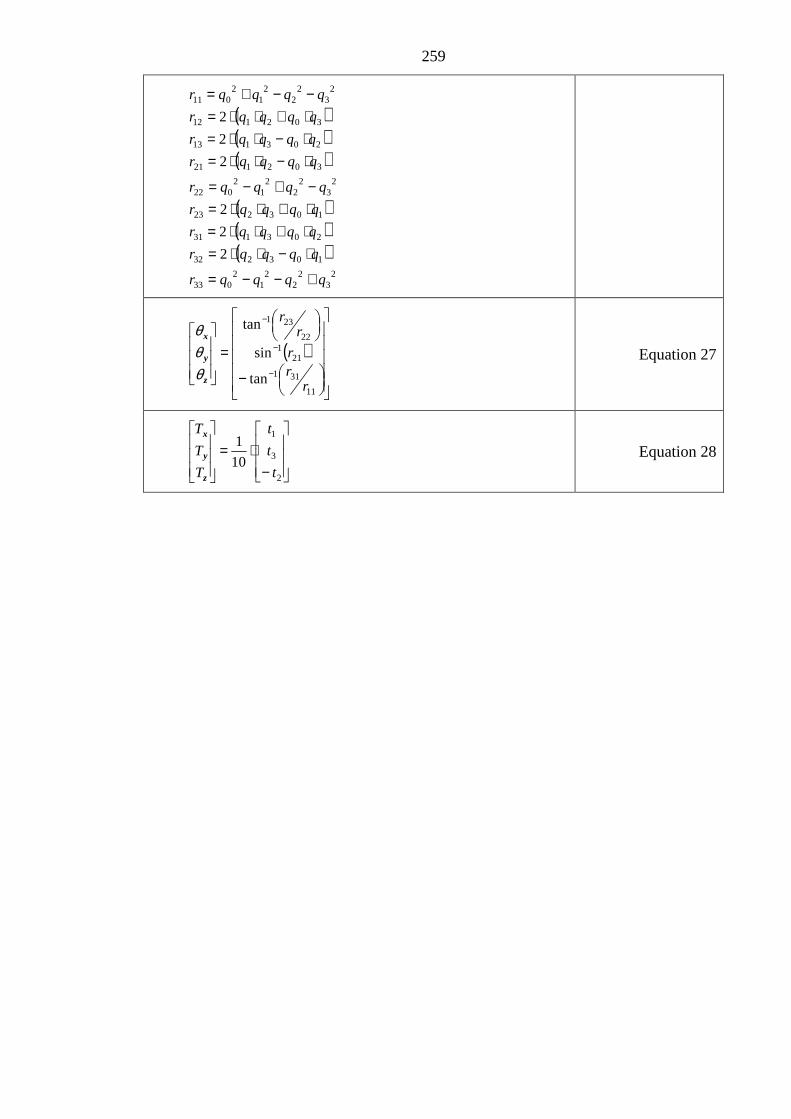
259

( )( )( )

( )( )( )

23

22

21

2033

103232

203131

103223

23

22

21

2022

302121

203113

302112

23

22

21

2011

2

2

2

2

2

2

qqqqr

qqqqr

qqqqr

qqqqr

qqqqr

qqqqr

qqqqr

qqqqr

qqqqr

+−−=

⋅−⋅⋅=⋅+⋅⋅=⋅+⋅⋅=−+−=

⋅−⋅⋅=⋅−⋅⋅=⋅+⋅⋅=−−+=

( )

−

=

−

−

−

11

311

211

22

231

tan

sin

tan

rrr

rr

z

y

x

θθθ

Equation 27

−⋅=

2

3

1

10

1

t

t

t

T

T

T

z

y

x

Equation 28

260

Table 22. Residual errors between measured and applied transforms in versor notation when the reference CT image is transformed and the localisation CBCT is of the phantom in its reference position. The last column shows the TRE50 (at a radius of 50mm) for these residual errors.

Rotation (°) Translation (mm)

Reference Pitch Yaw Roll Lat Vert Long TRE50

Transform q1 q2 q3 t1 t2 t3 (mm)

1a 0.002 -0.004 -0.002 0.11 0.89 0.50 1.06

1b 0.002 -0.002 -0.002 0.22 -0.01 0.33 0.44

1c 0.001 -0.003 -0.002 0.24 -0.42 0.32 0.63

1d -0.002 -0.004 -0.002 0.31 -0.27 0.01 0.56

1e 0.001 -0.003 -0.002 0.19 -0.04 0.02 0.35

1f 0.006 -0.004 -0.002 0.18 0.06 0.48 0.73

1g 0.000 -0.004 -0.002 0.29 0.02 0.35 0.55

1h 0.002 -0.003 -0.004 0.11 0.01 0.12 0.41

1j -0.002 -0.004 -0.002 0.09 -0.06 0.21 0.41

261

Table 23. Residual errors between measured and applied transforms in versor notation when the localisation CBCT image is transformed and the reference CT image is in the untransformed position. The last column shows the TRE50 (at a diameter of 50mm) for these residual errors.


Reference Pitch Yaw Roll Lat Vert Long TRE50

Transform q1 q2 q3 t1 t2 t3 (mm)

1a -0.002 -0.004 -0.002 0.40 -0.23 0.29 1.02

1b -0.006 -0.003 -0.002 0.12 -0.09 -0.40 1.07

1c -0.003 -0.005 -0.001 0.39 0.10 -0.04 0.96

1d 0.002 -0.005 -0.001 0.26 -0.18 0.10 0.77

1e -0.006 -0.002 -0.002 0.11 -0.12 0.18 0.87

1f -0.005 -0.006 -0.001 0.40 0.04 -0.08 1.13

1g -0.003 -0.004 0.000 0.36 0.01 -0.06 0.85

1h 0.000 -0.002 -0.002 0.47 0.30 -0.05 0.86

1j -0.005 -0.002 -0.002 0.11 0.00 -0.23 0.82

In chapter 5, the transformation of the CT images and CT-CBCT image

registrations are checked independently using the 27 external fiducial markers on the

surface of the VHMP phantom. The method of Arun et al was used to find a least

squares solution to corresponding markers [200].

Given two sets of points p1 and p2 in 3ℜ the rotation matrix can be found by single

value decomposition of the product p1.p2 as follows.

( )tt2

t1

t

t

21

222

111

pXpt

UVR

VUH

qqH

ppq

ppq

⋅−=

⋅=

=

⋅′=−=−=

Λ Equation 29

262

where the overscore represents the vector mean of the set of vectors representing

the coordinates of the points, and is only defined if 1)det( =R .

Table 24 shows the transforms measured using the 27 fiducial markers on the

surface of the VHMP phantom. The transforms were measured between the

untransformed CT image and the CT images transformed using test transforms 1a-1j

with the ITK VersorRigid3Dtransform class. The transforms compare well with the

applied transforms (Table 19). The residual errors of the transform and corresponding

TRE50 are shown in (Table 25). The coordinates of each of the fiducial points were

measured using the Synergy® XVI software and the uncertainty of the measurement was

estimated to be approximately ±0.5mm in each of the X, Y and Z directions. The last

column of Table 25 gives the mean residual distance (MRD) between the

untransformed sets of fiducials and the transformed fiducials having transformed back

with the measured transform. The MRD indicates the combined uncertainty of

localising each of the fiducials in the two image sets. The average MRD is 1.1 mm

which is equivalent to a standard deviation of 0.5mm on the localisation of each

fiducial.

263

Table 24. Transforms in VersorRigid3Dtransform format measured using the 27 fiducial markers on CT reference images of the VHMP phantom transformed using test transforms 1a-1j.


Reference Pitch Yaw Roll Lat Vert Long


1a -0.0008 -0.0004 0.0881 7.00 14.19 19.86

1b 0.0874 -0.0003 0.0002 7.36 13.98 19.88

1c 0.0005 0.0859 -0.0001 7.17 14.00 19.85

1e -0.0001 0.0865 0.1307 7.02 13.96 19.72

1f 0.0867 0.1300 0.0007 7.04 13.91 19.86

1g 0.0866 -0.0007 0.1307 7.17 14.07 20.02

1d 0.0209 0.0312 0.0433 7.62 13.88 20.06

Table 25. Residual errors between the transforms measured using the 27 fiducial markers on the VHMP phantom and those used to transform the CT images with test transforms 1a-1j. The last column shows the mean residual distance between the points when transformed with the test transform and the same points transformed with the measured transform.

Rotation (°) Translation (mm) TRE50 MRD

Reference Pitch Yaw Roll Lat Vert Long (mm) (mm)


1a 0.0008 0.0003 -0.0010 -0.04 -0.18 0.14 0.25 0.97

1b -0.0002 0.0003 -0.0002 -0.36 0.04 0.12 0.39 1.17

1c -0.0005 0.0013 0.0000 -0.20 0.00 0.12 0.25 0.96

1e 0.0002 0.0007 -0.0001 -0.05 0.05 0.27 0.29 1.06

1f 0.0005 0.0004 -0.0006 -0.07 0.11 0.11 0.18 1.20

1g 0.0007 0.0006 -0.0002 -0.18 -0.03 -0.01 0.19 1.12

1d 0.0009 0.0015 0.0003 -0.60 0.17 -0.11 0.64 1.36

Appendix B

Metrics for evaluation of similarity measure rigid

body parameter space

B.1 Metrics for evaluation of similarity measure profiles

In the papers by Skerl et al. [146,171] several metrics for evaluation of cost

functions (similarity metrics) are defined. These definitions have been slightly modified

and are presented here to aid interpretation of this thesis.

Let the transform parameters for a registration between two images be X0 (q1, q2,

q3, t1, t2, t3) in versor notation. The similarity metric at this position is SM0(X0). A

profile, n, where n = 1,2,…N and N = 6, along a cardinal axis is measured at M+1

points, between –M/2 and M/2 with spacing xδ which, in this work is set to different

values for the translation and rotation axis. The similarity measure for profile n, is

given by ( )mnXSM ,0 m = -M/2,-M/2+ xδ ,…,M/2- xδ , M/2. This is normalised to the

interval [0,1]

( ) ( )min0max0

min0,0, SMSM

SMXSMXSM mn

mn −−

= Equation 30

Where min0SM and max,0SM are the minimum and maximum values of ( )mnXSM ,0

over all NM+1 positions. Let optnX , be the position of the global optima for profile n.

265

B.1.1 Accuracy (ACC)

As defined by Skerl et al. ACC is the root mean square of distances between the

origin and global optima for each profile (Equation 31.)

∑=

−=N

noptn XX

NACC

1

2

0,

1

Where, N is the number of profiles,

( ) ( )( )∑=

−=−6

1p0opt,n0opt,n pXpXXX

Equation 31

and p =1,2,…,N represents the parameter of the rigid body rotation.

In Chapter 8, profiles are only calculated along the six primary and orthogonal axis

of the parameter space. Without any diagonal profiles, as in the work of Skerl et al., it

was not necessary to normalise the parameter space so that increments of rotation had

equal effect to increments of translation. Since the parameter space was not normalised

it was logical to split the measure of accuracy into separate definitions for translational

accuracy (ACC_T) and rotational accuracy (ACC_R). This led to the definitions of

ACC_T and ACC_R in Equation 32 and Equation 33.

( ) ( )( )23

1p0opt,n pXpX

3

1T_ACC ∑

=

−= Equation 32

( ) ( )( )26

4p0opt,n pXpX

3

1R_ACC ∑

=

−= Equation 33

B.1.2 Risk of non-convergence (RON)

The risk of non convergence (RON) of the optimum is a metric that describes the

shape of the SM in the locality of the global minimum. Risk of non-convergence is

defined by Skerl et al, for a particular profile, as the average of all positive gradients of

the normalised SM out to a distance r, from the position of the minimum. These values

are then averaged over all profiles sampled. A low value of RON indicates a broad

266

minima with shallower gradients whereas a narrow minima with steep gradients has a

high value of RON. To calculate RON, first the positive gradients are calculated

(Equation 34).

( ) ( ) ( ) ( )( ) ( ) ( ) ( )

><−><−

= ++

−−

otherwise0

XSMXSM&optmifXSMXSM

XSMXSM&optmifXSMXSM

d m,n1m,nm,n1m,n

m,n1m,nm,n1m,n

m,n

where n = 1,2,…N the number of profiles, m is an index to the calculation point along the profile an opt is the index to the position

along the profile at which the minimum value is found.

Equation 34

RON is then given by

∑ ∑=

+

−−=

=N

1n

sopt

soptmm,nd

r2

1)r(RON Equation 35

In chapter 8, RON was split into two components: RON_T was defined as the

mean risk of non convergence for profiles along the translation axis and RON_R was

the mean risk of non convergence for profiles along the rotation axis. In this case we

redefine RON as function of n in Equation 36 and calculate the individual RON_T and

RON_R components using Equation 37 and Equation 38.

∑+

−−=

=sopt

soptmm,nd

r2

1)n,r(RON Equation 36

∑=

==2

1n

)n,mm1r(RONr2

1T_RON Equation 37

∑=

==6

4n

)n,5.0r(RONr2

1R_RON o Equation 38

B.1.3 Distinctiveness of optimum (DO)

As the name suggests DO describes the distinctiveness of the optimum. For a

particular profile it is the average difference in normalised SM between points

equidistant from the global optimum at a distance r from the minimum divided by the

distance. These values are then averaged for all profiles. It was defined by Skerl et al,

267

by Equation 39 for a profile n, at a distance r from the origin X0 where xsr δ.= and s =

1,2,…..

( ) ( ) ( ){ }∑=

+− −−⋅=N

1nropt,nropt,nopt,n XSMXSMXSM2

rN2

1)r(DO Equation 39

In the work of Skerl et t al., DO was summed over all n and the position, r, at

which DO was calculated was not defined. As with accuracy, DO was split into

translation and rotation components in chapter 8. DO was redefined as a function of n

(Equation 40) before summing over either the translation parameters (Equation 41) or

the rotation parameters (Equation 42). The position, r was set to 1mm or 0.5°.

( ) ( ) ( ){ }ropt,nropt,nopt,n XSMXSMXSM2r2

1)n,r(DO +− −−⋅= Equation 40

∑=

==3

1n

)n,mm1r(DO3

1T_DO Equation 41

∑=

==6

4n

)n,5.0r(DO3

1R_DO o Equation 42

B.2 Metrics for evaluation of sub-sampled (25 point) similarity metric

profiles

A set of nine metrics were devised for analysis of the 25 values of the similarity

metric calculated at X0 ±1mm and ±2mm from X0 along each of the three translation

axis and also at ±0.5° and ±1° along the rotation axis, where X0 is the position returned

by the image registration algorithm. IsMin25, ∆Xmin,25, SM25(Xmin,25), ∆Xfit,25 &

SM25(X0) are adequately described in chapter 8. The others warrant further description.

B.2.1 Distinctiveness of Optimum DO25(1), DO25(2) & DO25(Av)

This is defined very similarly to the DO defined by Skerl et al but with fewer

points. DO25(1) is the absolute gradient between the similarity metric at the 12 inner

268

points, located at ±1mm and ±0.5° along the three translation and three rotation axis

relative to X0, and similarity metric at X0.

( ) ( ) 12XSMXSM)1(DOptsinner

inner025 ∑−= Equation 43

DO25(2) is the absolute gradient between the similarity metric at the 12 outer

points, located at ±2mm and ±1° along the three translation and three rotation axis

relative to X0, and similarity metric at X0

( ) ( ) 212XSMXSM)2(DOptsouter

outer025

−= ∑ Equation 44

DO25(Av) is the mean of , was the average of DO25(1) and DO25(2).

B.2.2 Minimum Value, ∆∆∆∆Xmin,25

∆Xmin,25, was the position of the lowest of the 25 similarity metric samples relative

to X0. ∆Xmin,25 takes values of 0, 1 & 2 if the minimum was located at X0, at one of the

inner points or at one of the outer points respectively.

B.3 Quadratic fit to calculate ∆∆∆∆X25,fit and SM25(X25,fit)

The position of the global minimum can be estimated by performing a quadratic

curve fit to the 25 points. This was performed using least squares regression as follows.

Let 2525 .)( XXBXSM = where SM is the similarity metric calculated at the 25

points X25 and XX25 is the design matrix. In this work XX25 is defined as follows.

( ) ( ) ( ) ( ) ( ) ( ) ( ) ( ) ( ) ( ) ( ) ( )( ) ( ) ( ) ( ) ( ) ( ) ( ) ( ) ( ) ( ) ( ) ( )( ) ( ) ( ) ( ) ( ) ( ) ( ) ( ) ( ) ( ) ( ) ( )2525252525252525252525251

2222222222221

1111111111111

222222

222222

222222

25

zyxzyxzyxzyx

zyxzyxzyxzyx

zyxzyxzyxzyx

TTTTTT

TTTTTT

TTTTTT

XX

θθθθθθθθθθθθθθθθθθ

=

The coefficients B can be found using Equation 45

269

( ) ( )25252525 XSMXXXXXXB ⋅′⋅′⋅′= Equation 45

To determine the position of the global minimum we need to differentiate

2525 .)( XXBXSM = with respect to each parameter (Equation 46).

=∆

13

7

12

6

11

5

10

4

9

3

8

2,25 B

B

B

B

B

B

B

B

B

B

B

BX fit Equation 46

SM25(X25,fit) is simply the similarity metric calculated at X25,fit.

Examples of the quadratic regression model are shown in Figure 45.The

regression works well in most cases.

270

−1 0 1

−0.9

−0.895

−0.89

−0.885

−0.88

Shift deg

CR

Pitch

−1 0 1

−0.9

−0.895

−0.89

−0.885

−0.88

Shift deg

CR

Roll

−1 0 1

−0.9

−0.895

−0.89

−0.885

−0.88

Shift deg

CR

Yaw

−0.2 0 0.2

−0.902

−0.901

−0.9

−0.899

−0.898

Shift cm

CR

Lat

−0.2 0 0.2

−0.902

−0.901

−0.9

−0.899

−0.898

Shift cm

CR

Vert

−0.2 0 0.2

−0.902

−0.901

−0.9

−0.899

−0.898

Shift cm

CR

Long

−1 0 1

−0.895

−0.89

−0.885

−0.88

−0.875

−0.87

Shift deg

CR

Pitch

−1 0 1−0.895

−0.89

−0.885

−0.88

−0.875

−0.87

Shift deg

CR

Roll

−1 0 1−0.895

−0.89

−0.885

−0.88

−0.875

−0.87

Shift deg

CR

Yaw

−0.2 0 0.2

−0.8955

−0.895

−0.8945

−0.894

−0.8935

−0.893

−0.8925

−0.892

Shift cm

CR

Lat

−0.2 0 0.2

−0.8955

−0.895

−0.8945

−0.894

−0.8935

−0.893

−0.8925

−0.892

Shift cm

CR

Vert

−0.2 0 0.2

−0.8955

−0.895

−0.8945

−0.894

−0.8935

−0.893

−0.8925

−0.892

Shift cm

CR

Long

−1 0 1−0.71

−0.7

−0.69

−0.68

−0.67

−0.66

Shift deg

CR

Pitch

−1 0 1−0.71

−0.7

−0.69

−0.68

−0.67

−0.66

Shift deg

CR

Roll

−1 0 1−0.71

−0.7

−0.69

−0.68

−0.67

−0.66

Shift deg

CR

Yaw

−0.2 0 0.2−0.684

−0.682

−0.68

−0.678

−0.676

−0.674

Shift cm

CR

Lat

−0.2 0 0.2−0.684

−0.682

−0.68

−0.678

−0.676

−0.674

Shift cm

CR

Vert

−0.2 0 0.2−0.684

−0.682

−0.68

−0.678

−0.676

−0.674

Shift cm

CR

Long

−1 0 1

−0.71

−0.7

−0.69

−0.68

−0.67

−0.66

Shift deg

CR

Pitch

−1 0 1−0.71

−0.7

−0.69

−0.68

−0.67

−0.66

Shift degC

R

Roll

−1 0 1−0.71

−0.7

−0.69

−0.68

−0.67

−0.66

Shift deg

CR

Yaw

−0.2 0 0.2−0.684

−0.682

−0.68

−0.678

−0.676

−0.674

Shift cm

CR

Lat

−0.2 0 0.2−0.684

−0.682

−0.68

−0.678

−0.676

−0.674

Shift cm

CR

Vert

−0.2 0 0.2−0.684

−0.682

−0.68

−0.678

−0.676

−0.674

Shift cm

CR

Long

Figure 45. Examples of the quadratic fit to the similarity metric profiles. The Solid

dark blue line shows the measured SM while a red cross indicates one of the

25 sampled points. The dotted light blue line shows the results of the

quadratic curve fit.

Quantification of Geometric Uncertainties in Image Guided...

Documents

Transcript of Quantification of Geometric Uncertainties in Image Guided...