Quantification of Condition Monitoring Benefit for Offshore Wind...

Quantification of Condition Monitoring Benefit forOffshore Wind Turbines

by

David McMillan and Graham W. Ault

REPRINTED FROM

WIND ENGINEERINGVOLUME 31, NO. 4, 2007

MULTI-SCIENCE PUBLISHING COMPANY5 WATES WAY • BRENTWOOD • ESSEX CM15 9TB • UKTEL: +44(0)1277 224632 • FAX: +44(0)1277 223453E-MAIL: [email protected] • WEB SITE: www.multi-science.co.uk

Quantification of Condition Monitoring Benefit forOffshore Wind Turbines

David McMillan and Graham W. AultInstitute for Energy & Environment, University of Strathclyde, Royal College Building, 204 GeorgeStreet, Glasgow, G1 1XWEmail <[email protected]>, <[email protected]>

WIND ENGINEERING VOLUME 31, NO. 4, 2007 PP 267–285 267

ABSTRACTCondition monitoring (CM) systems are increasingly installed in wind turbines with the goal

of providing component-specific information to wind farm operators, theoretically

increasing equipment availability via maintenance and operating actions based on this

information. In the offshore case, economic benefits of CM systems are often assumed to be

substantial, as compared with experience of onshore systems. Quantifying this economic

benefit is non-trivial, especially considering the general lack of utility experience with large

offshore wind farms. A quantitative measure of these benefits is therefore of value to utilities

and operations and maintenance (O & M) groups involved in planning and operating future

offshore wind farms. The probabilistic models presented in this paper employ a variety of

methods including discrete-time Markov Chains, Monte Carlo methods and time series

modelling. The flexibility and insight provided by this framework captures the necessary

operational nuances of this complex problem, thus enabling evaluation of wind turbine CM

offshore. The paper concludes with a study of baseline CM benefit, sensitivity to O & M costs

and finally effectiveness of the CM system itself.

Keywords: Wind Farms, Condition Monitoring, Operations and Maintenance, Markov

Chain, Monte Carlo, Probabilistic Model.

NOMENCLATURECM Condition Monitoring

SCADA Supervisory Control Alarm and Data Acquisition

CBM Condition Based Maintenance

WT Wind Turbine

O & M Operation and Maintenance

F Annual Maintenance Frequency

R WT Revenue

MWhT Mega-Watt Hours Generated During Time Period T

MPROC Market Price of Renewable Obligation Certificates

MPELEC Market Price of Electricity

Pr(event) Probability of Occurrence of an Event

Im(event) Impact of Event

L Confidence Limit

s Standard Deviation of Sample

N Number of Samples

WSt Wind Speed at Time t

Wind 31-4_final 7/11/07 3:06 pm 67

WSt-1 Wind Speed at Time t-1

µ Mean Wind Speed

ø Autoregressive Model Parameter

εt Gaussian Error Term

σ2 Variance of Gaussian Error Term

Z Z score for Gaussian Distribution

1. INTRODUCTIONGlobal concerns regarding energy security, alongside increasing public acceptance of human

influence on global warming have motivated a recent surge in support for renewable energy

technologies. Wind Farms have emerged as the technology regarded by most policy makers

and utilities as the renewable energy source most suited to delivering desired targets on

carbon emission reductions and diversity of supply. The long term focus in the UK and

elsewhere is gradually switching from onshore to offshore, because of less problematic visual

intrusion and significantly higher yields due to larger WT ratings and stronger wind profiles.

Large projects such as the proposed 1 GW London Array [1], 0.5 GW Greater Gabbard [2] and

0.25 GW Lincs [3] have illustrated substantial interest and growth potential in this area.

Various forms of condition monitoring (CM) systems have become increasingly common

as part of the turbine Supervisory Control Alarm and Data Acquisition system (SCADA

system). The theoretical benefits of such systems are well known, and indeed these benefits

have already been realised by operators of traditional generating sets (gas, coal etc.). The CM

information is utilised to detect incipient faults, thus enabling more effective and efficient

maintenance scheduling (as compared to the well known and oft-used periodic maintenance

policy). However it must be noted from the operational viewpoint that any prospective

maintenance policy based on condition information must have clear economic benefits;

otherwise the initial outlay for the CM system and associated costs cannot be justified.

Large offshore wind farms have their own distinct characteristics which further challenge

widely held assumptions with respect to CM applied to wind turbines. A commonly held

assumption is that CM systems will become cost effective for offshore wind farms, due to a

number of factors:

● Increased lost energy, and hence lost revenue, due to larger capacity ratings of

offshore turbines and stronger wind profiles

● Longer downtimes (harsh weather, large distances involved, modes of transport

required)

● Larger, heavier, more costly components for larger capacity rated turbines

designed for the offshore environment, requiring higher outlay for O&M

The research presented in this paper aims to address these issues via a framework of

highly flexible probabilistic models which are capable of capturing the subtleties of wind farm

operational activities. These models are informed both by the literature and by direct

dialogue with Scottish Power PLC: a utility involved in operation and maintenance of an

extensive wind farm portfolio.

The paper proceeds as follows. Section 2 provides a summary of existing research upon

which this work is built. Section 3 gives an extensive overview of the models used to quantify

offshore WT CM system benefit, as well as the sources of information used to guide and

populate those models. Section 4 presents a set of case studies designed to investigate the cost

268 QUANTIFICATION OF CONDITION MONITORING BENEFIT FOR OFFSHORE WIND TURBINES

Wind 31-4_final 7/11/07 3:06 pm Page 268

effectiveness of offshore WT CM. Section 5 draws some conclusions from the results and

suggests possible implications for offshore wind farms.

2. WIND TURBINE CONDITION MONITORING AND MODELLING Most modern wind turbines are now manufactured with some form of integrated CM system,

interfaced to the operator via a Supervisory Control Alarm and Data Acquisition System

(SCADA system). Such CM systems are commonly based on vibration monitoring of the WT

drive-train as well as temperature measurement of bearings, machine windings etc. [4] and [5]

provide particularly insightful reviews of the state of the art in WT CM systems. Additionally,

several emerging systems [6] are commercially available based on technologies such as

lubrication oil particulate content and optical strain measurements. Various other systems

have been proposed in literature, such as the blade monitoring system presented in [7], and the

holistic set of intelligent models developed in [8]: however, temperature and vibration are the

main condition monitoring tools used in commercially available systems.

Published research has shown that via different approaches, the benefit of a condition-

based maintenance scheme for onshore wind farms can be quantified. Andrawus et al. [9]

compiled detailed costs and extracted sub-component failure rates from 6 years of wind

turbine SCADA data, with the goal of deciding a suitable maintenance strategy. A

combination of reliability-centred maintenance and asset life-cycle analysis was used, and

Monte Carlo Simulation was employed to introduce uncertainty into key variables. This

approach suggested that, for the conditions evaluated, a Condition Based Maintenance (CBM)

strategy is the most cost-effective option. The total savings of £180,152 were discounted using

net present value, and equate to an annual saving of £385 per turbine over the 18 year life

cycle of a 26 turbine onshore wind farm. A contrasting approach by the authors of this paper

[10] brought together a set of models representing physical component condition (based on a

Markov Chain solved via Monte Carlo Simulation), turbine yield and asset management

objectives. The problem was formulated and populated with data from various sources,

including published data and anecdotal evidence from Scottish Power. Maintenance models

were developed and the output validated using simple calculations. Probabilistic simulations

were run in order to compare the performance of two maintenance policies (periodic and

condition-based) and thus quantify the benefit of WT CM. The results indicated that while a

mean yearly benefit of £2,000 was calculated in favour of CBM, the confidence limits were

such that the case for onshore condition-based maintenance of WTs appeared to be uncertain.

The work contained in this paper builds on the previous work by the authors, modifying

the models to reproduce offshore conditions. The strength of this approach is its flexibility:

data from a variety of sources are taken advantage of, and since experience of large offshore

wind farms is limited, the results enable insight for owners and operators of future large

offshore wind farms.

Given that the CM system is monitoring the status of a set of components, capturing the

deterioration process of those components is a vital part in any maintenance simulation.

When this process is adequately represented, condition monitoring can be modelled as

knowledge of the current state. Research related to this area of ‘deterioration modelling’ and

maintenance modelling exists in literature, with many interesting applications, providing

useful insight for this work. Marseguerra [11] and Baratta [12] approach the problem as a

discrete event simulation: the Markov Chain deterioration model represents key components

in the nuclear safety sector. Both sets of authors identify an optimal deterioration threshold

limit (in terms of availability and profit) at which condition-based maintenance should be

WIND ENGINEERING VOLUME 31, NO. 4, 2007 269


conducted: however while Baratta uses sensitivity studies, Marseguerra uses a genetic

algorithm to achieve the optimisation. Endrenyi and associates have published a number of

influential contributions on deterioration modelling and the effects of maintenance including

[13] and [14]. Sayas and Allan [15], as well as Billinton [16], have both developed wind turbine

models for use in reliability studies: although these understandably neglect intermediate

states. Markov models have been applied successfully by a number of authors in asset

management applications, with insightful contributions in the fields of oil-filled circuit

breakers [17], water infrastructure [18], and road networks [19].

Continuous-time models with analytical solution are favoured by most authors: however

this can be problematic when representing more complex systems and processes due to a

lack of flexibility in the modelling framework. Discrete-time models solved via simulation

provide a degree of insight and flexibility which is essential to capture the nuances of

operational activities, since the problem does not have to be expressed in closed-form

equations. Therefore, a discrete-time simulation-solved model is adopted in this work.

3. WIND TURBINE ASSET MANAGEMENT MODELLINGIn order to represent the various facets of the complex problem of quantifying the effects of

CM on WTs, a multi-level modelling approach is being adopted, as shown in Figure 1. The three

levels enable a diverse range of processes to be effectively modelled such as physical

deterioration and faults, wind farm yield modelling and weather effects, and high-level asset

management decisions: these individual aspects are now discussed.

3.1 Wind Turbine Sub-Component ModelThe sub-component representation of a physical system has been implemented in several

different ways in literature, as shown in Figure 2. Moving from left to right, the two-state

representation such as that used in older reliability studies is unsuitable for this application as

it does not consider the ‘derated’ or deteriorated states which the CM system can infer over

time (refer to Figure 6 for an example). The single component approach (centre) would

require parallel simulation to solve: this should be avoided as far as possible due to the chance

of introducing undetected simulation correlations causing bias in the result [20]. Thus the

multi-component, intermediate state model (right) is adopted for this work.


Figure 1. Multi-level WT Asset Management Modelling Framework

Figure 2. Sub-Component Models


The next stage is to decide which components should be considered in the analysis, and

how the component states map to the measured condition variables provided by the CM

system. Both of these issues are very important, having a significant impact on the model

accuracy. Two main sources of information were used to determine which of the WT sub-

components should be included in the modelling: published sub-component reliability data;

and wind farm operational experience. Once these issues are addressed, the state-space of the

Markov model is effectively defined.

3.2 Wind Turbine Sub-Component Reliability DataReliability data for wind turbine sub-components are collected by some turbine operators, but

are not readily available in the public domain. When available to researchers, this information

(although limited)represents a useful starting point for modelling the wind turbine sub-

components, ultimately for use in the condition monitoring evaluation study. A summary plot

of three studies containing WT sub-component reliability data are shown in Figure 3: these

have been taken from various published sources (Left to right: [21], [22] and [23]).

The data plotted in Figure 3 are predominantly characteristic of the experiences of Danish

and German utilities. Many failures are electronic related, with small downtime although

replacement or repair in the offshore environment is likely to be more time-consuming than

on land. Indeed, it is important to note that these results reflect only relative failure frequency:

not duration of downtime, or cost of components. Hence, other factors beyond the failure rate

should be considered.

3.3 Wind Farm Operational ExperienceDialogue with a Scottish Power yields interesting contrast with published results as outlined in

the previous section. It is clear through this dialogue that the most significant operational

failures are associated with the gearbox and generator components. The reasons are:

● High capital cost and long lead-time for replacement

● Difficulty in repairing in-situ

● Large physical size and weight

● Position in nacelle at top of tower

● Lengthy resultant downtime, compounded by adverse weather conditions

The final point can be reinforced when it is understood that typical downtime for an


Figure 3. Causes of WT Failures in Published Studies


unscheduled gearbox replacement is of the order of 700 hours [24], though this is dependent

on availability of the component from the manufacturer. A recent report detailing operational

activities at the Scroby Sands offshore wind farm [25] appears to back up the conclusions

above, with gearbox bearing problems the most prevalent. Published data available from

windstats [26], and plotted in Figure 4, shows the significance of operational failures in terms

of downtime per component failure. This data reinforces the conclusions above, since the

generator and gearbox failures account for 42% of the total downtime.

Taking this information into account, the studies conducted in this paper feature a

4–component model comprising generator, gearbox, blades and power electronics system.

The gearbox and generator were included for the reasons outlined above by the industrial

project partners. Blades were also included as there are emerging methods of monitoring

these, and while they have low probability of failure, the impact of a blade replacement is very

significant from an operational and economic viewpoint. Finally, in order to accurately re-

create the overall wind turbine failure rate, power electronics was included even though

monitoring capability is not modelled.

Figure 5 illustrates the four WT sub-components and a sub-set of monitoring options. The

quality of information provided by each of these measurements, as well as the data

interpretation, determines the accuracy of the overall ‘system picture’, as inferred by the CM

system.

3.4 Mapping of CM Information to Markov StatesThe crux of condition monitoring effectiveness lies in the ability of the CM system to reliably

diagnose the status of the components and hence the overall system. There are of course

many methods of achieving this, some more simple than others. This ability to diagnose and

categorise (whether achieved via human expert or automated systems) is the basis of any

CM system and its subsequent mathematical representation. Indeed, the practicalities of

quantifying condition as a mathematical index have been investigated elsewhere: a

particularly comprehensive and succinct summary is provided in [27]. For this work, a simple

example of the possible mapping between the monitored system variables and Markov state

space is sufficient to illustrate the concept.


Figure 4. WT Downtime Distribution [26]


Figure 6 shows a set of wind turbine gearbox lubrication oil temperature traces, along with

possible state categorisation. Since deterioration is essentially random, Monte Carlo methods

can be used to represent this process adequately. It can be seen that the physical state of the

WT component corresponds to its modelled state in the Markov chain (e.g. fully up, derated,

failed). The components to be modelled are those shown in Figure 5: the states of those

components may be categorised in the manner shown in Figure 6, using the various CM

methods available. Finally, the state-space must be defined based on this information, and the

transition probabilities between states deduced.

3.5 Markov Chain State SpaceIn the state space diagram, each box represents the condition of the overall wind turbine, i.e.

the status of the 4 modelled components. Figure 7 shows the full state space where C1, C2, C3

and C4 represent the modelled components and their various possible condition states. The

total possible state space is 52 states: however this was reduced to 28 via simplifying

assumptions, the most influential being that probability of simultaneous failure events is

considered insignificant and that components will transit to a derated state before outright

failure (except electronics). The model time resolution is 1 day, which does represent a highly

optimistic picture of the ability of the CM system to catch failures before they occur. The

validity of these assumptions increases as the time resolution of the model approaches

continuous time i.e. small discrete intervals of minutes rather than days. Future studies will

take account of near-instantaneous failure events as these are not currently explicitly

modelled, though the framework is amenable to such changes. A deeper study of the early

warning capability of WT CM systems and the nature of offshore WT faults (i.e. time periods

involved) would be the next step in refining the approach. For the results contained in this

paper, however, the 1 day time resolution model is used.


Figure 5. Selection of WTG Monitoring Options

Figure 6. CM System Categorisation


3.6 Transition Probability Matrix Ideally the transition probability matrix which governs the behaviour of the system over the

discrete intervals would be defined by taking a long-run turbine history and calculating

transitions based on this history alone. The main issue is that such data sets may not exist in

reality, and may not capture a wide range of turbine faults: therefore other approaches must

be considered.

The sub-component failure probabilities (see 3.2) are known quantities over large

populations of turbines, and therefore the model should reproduce these faithfully (if sampled

sufficiently to reach steady-state values). The transition probabilities can be at least partially

deduced by using sensitivity studies to observe the effect on these model output metrics

compared with actual sub-component failure rate values. Additionally, the probabilities can

be influenced by comparing the model condition trajectory to that of a real monitored turbine

in operation (see Figure 6). For example, it is possible to deduce the probability of failure in the

next time period if it is known that the current state is a de-rated state: in this sense the turbine

condition data provides direct input into shaping the behaviour of the model. It should be

noted however that minor outages are often not recorded in the available statistical data:

therefore in reality the failure rate may be higher than suggested in such publications. This

may be a significant factor offshore, since even a minor shutdown may necessitate an

inspection and associated costs, which may be substantial.

3.7 Turbine Yield ModelThe yield model consists of two parts: a power curve model and a wind speed model. The wind

model is based on an autoregressive time series model with a single parameter (also known

as an AR(1) model). This has been developed using raw SCADA data from an onshore WT at

Black Law wind farm with a strong wind profile (mean wind speed, µ, 7m/s), to reproduce

offshore performance as closely as possible, given the limited data available offshore.

Although offshore locations may have significantly stronger wind regimes, this profile

represents the best case with the data available. The single parameter autoregressive model

has the form:

(1)

If the wind speed in the previous period, WSt-1, is known, then the next time series value,

WSt, can be calculated from equation (1). Classification was achieved through inspection of

WSt – m = f (WSt–1 – m) + et


Figure 7. WT Condition State Space Diagram


the autocorrelation and partial autocorrelation functions [28], and the model was fitted using

the ordinary least squares fitting technique. A statistical programming language was used to

estimate model parameter ø and variance σ2 of the Gaussian noise term εt. This approach

enables day to day correlation between wind speed values to be captured within the model.

Simulated wind speed values can thus be plugged into the relevant power curve, as shown in

Figure 8. This is a 5 MW rated machine [29], specifically developed for offshore applications. It

has characteristic cut in, rated and cut out wind speeds of 3.5, 13 and 30 m/s respectively.

Turbine revenue, R, is calculated from the energy (MWh) generated, and is calculated as

shown in eq’n (2), where MPElec and MPROC, the market price of electricity and renewables

obligation certificates, are taken as £36/MWh and £40/MWh respectively. These costs are

currently fixed in the model, although their variability could easily be modelled

deterministically or probabilistically in future studies. Operations and maintenance costs,

described in the next section, are subtracted from the revenue stream to calculate income

from each turbine.

(2)

3.8 Maintenance ModelsTwo contrasting maintenance approaches were implemented in the model: periodic and

risk/condition based maintenance.

● Periodic – Perform maintenance at set intervals (~Every 12 months)

● Risk/Condition Based – Maintain according to condition rule policy

It is noted that both approaches will inevitably involve some reactive maintenance,

especially in the offshore case where frequent periodic maintenance is often impractical.

Additionally, many maintenance and repair actions will be subject to weather constraints for

offshore installations. Table 1 illustrates a set of maintenance restrictions as applied onshore,

set by the owner/ operator for health and safety reasons: these restrictions are built into the

program. Until data for offshore access and working arrangements is available, Table 1 will be

adopted for use in the offshore analysis. Although wave height is the dominant access factor

offshore, this is coupled strongly with wind speed and so inclusion of wind speed constraints is

valid, though clearly this represents an approximation which may have an effect on the

results of the analysis.

R = MWhT × [MPElec + MPROC]Trials

T=1


0

1

2

3

4

5

Wind Speed m/s

Po

we

r O

utp

ut

MW

Figure 8. 5 MW Offshore Wind Turbine


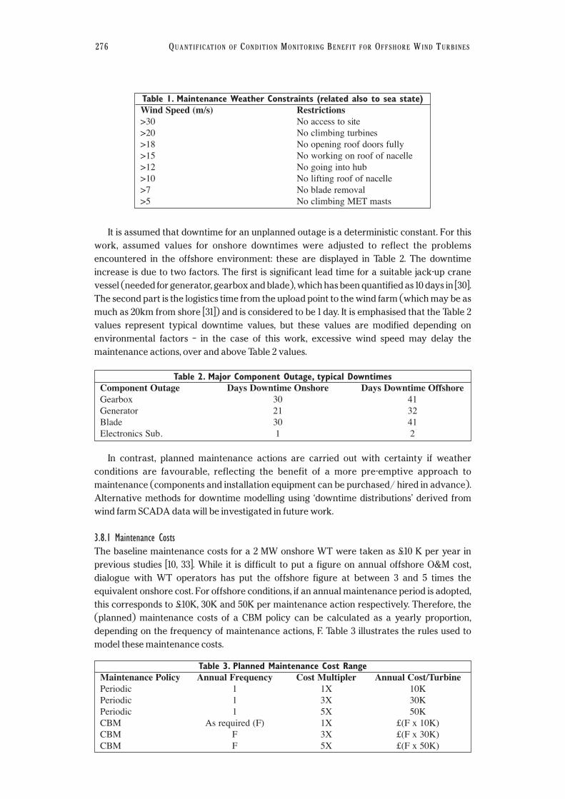
It is assumed that downtime for an unplanned outage is a deterministic constant. For this

work, assumed values for onshore downtimes were adjusted to reflect the problems

encountered in the offshore environment: these are displayed in Table 2. The downtime

increase is due to two factors. The first is significant lead time for a suitable jack-up crane

vessel (needed for generator, gearbox and blade), which has been quantified as 10 days in [30].

The second part is the logistics time from the upload point to the wind farm (which may be as

much as 20km from shore [31]) and is considered to be 1 day. It is emphasised that the Table 2

values represent typical downtime values, but these values are modified depending on

environmental factors – in the case of this work, excessive wind speed may delay the

maintenance actions, over and above Table 2 values.

In contrast, planned maintenance actions are carried out with certainty if weather

conditions are favourable, reflecting the benefit of a more pre-emptive approach to

maintenance (components and installation equipment can be purchased/ hired in advance).

Alternative methods for downtime modelling using ‘downtime distributions’ derived from

wind farm SCADA data will be investigated in future work.

3.8.1 Maintenance CostsThe baseline maintenance costs for a 2 MW onshore WT were taken as £10 K per year in

previous studies [10, 33]. While it is difficult to put a figure on annual offshore O&M cost,

dialogue with WT operators has put the offshore figure at between 3 and 5 times the

equivalent onshore cost. For offshore conditions, if an annual maintenance period is adopted,

this corresponds to £10K, 30K and 50K per maintenance action respectively. Therefore, the

(planned) maintenance costs of a CBM policy can be calculated as a yearly proportion,

depending on the frequency of maintenance actions, F. Table 3 illustrates the rules used to

model these maintenance costs.

Table 1. Maintenance Weather Constraints (related also to sea state)Wind Speed (m/s) Restrictions>30 No access to site>20 No climbing turbines>18 No opening roof doors fully>15 No working on roof of nacelle>12 No going into hub>10 No lifting roof of nacelle>7 No blade removal>5 No climbing MET masts

Table 2. Major Component Outage, typical DowntimesComponent Outage Days Downtime Onshore Days Downtime OffshoreGearbox 30 41Generator 21 32Blade 30 41Electronics Sub. 1 2

Table 3. Planned Maintenance Cost Range Maintenance Policy Annual Frequency Cost Multipler Annual Cost/TurbinePeriodic 1 1X 10KPeriodic 1 3X 30KPeriodic 1 5X 50KCBM As required (F) 1X £(F x 10K)CBM F 3X £(F x 30K)CBM F 5X £(F x 50K)



In addition to scheduled maintenance costs, unplanned costs for replacement of major WT

components should also be modelled, as they are significant. To capture this, every time the

Markov model transits to a failure state, the failed component is identified and repair or

replacement cost deducted from the WT revenue stream (of course any potential yield

revenue is also lost while in the down state). Estimated replacement costs for the key

components of an offshore 5MW WT are shown in Table 4, and are calculated using the

‘percentage of capital cost’ method proposed in [32]. Capital cost of £600,000 per MW of

installed capacity was assumed for the purposes of deriving component cost estimates [33]:

overall capital cost of offshore projects is currently closer to £1M per MW capacity. Repair

costs are taken as a 10% proportion of the offshore component replacement values.

These costs are modelled deterministically, but this is another area of the model where

increased detail could be accommodated in future developments of the model. Likewise, the

probability of repair or replacement of a failed component is equally likely: further study into

the robustness and ‘reparability’ of the components may lend more accuracy to these

assumptions.

3.8.2 Periodic Maintenance RegimeThe most widely practiced maintenance paradigm in any industry is periodic maintenance,

and maintenance of wind farms is no different. Despite the various monitoring options

available, most owner/ operators tend to keep to methods they are familiar with in

maintenance of their assets. In the model it is assumed that maintenance actions are 100%

successful, and have only a small impact on yield, being scheduled during periods of low wind.

The actions are weather constrained and are assumed to be carried out once every 12 months.

3.8.3 Condition Based Maintenance RegimeAs previously discussed, one of the chief advantages of the Markov approach is its ability to

model condition monitoring knowledge capture. In reality, the WT operator would observe

(manually or through an automated system) the trajectory of various instrumented WT

components via measurements delivered by the CM system, as previously discussed. In the

Markov model this can be replicated by allowing the maintenance actions to be informed by

the current state of the system (Physical Markov condition model): see Figure 9 for a simple

illustration of this concept.

Table 4. 5MW WT Component Replacement CostGearbox £402,000Generator £201,000Blade £166,000Electronics Sub. £10,000


Figure 9. Markov Model Captures Condition Monitoring Information


An implicit assumption in this approach is that the CM system can infer the current

equipment condition with certainty. Therefore, the model as defined so far does not address

the issue of possible spurious CM diagnosis. This shortcoming is addressed in section 4.3,

where a further refinement is added which allows possible unreliability of the CM system to

be modelled, and will be explored further in future work.

The next challenge is the development and specification of a suitable condition-based

decision model, coupling condition and maintenance. An operator of any plant or system

desires some signal regarding the risk that their plant is subject to. Risk is defined as the

product of probability and impact of an event or compound event: the Markov model is again

particularly suited to the expression of such metrics. The risk in any system state can be

expressed specifically as:

(3)

Where N failure events are possible, Pr(event) is the probability of transition to a failure

state and Im(event) is the impact of that particular component failure should it occur, which

could comprise a number of economic terms, but is currently simply the component

replacement cost. By using the equation above, all states with probability paths to failure can

have an associated risk calculated for them, as displayed in Figure 10. The reason only states

2-8 are included is that these are the intermediate operational states where the CM knowledge

can be utilised.

Once calculated, the magnitude of risk for each state can be used as an indicator to

determine how urgently repair work should be scheduled by the operator of the WT. In this

work the risk measure is used to set a maintenance time delay. The states are grouped into

intervals depending on their risk values: at this point there is no formal framework for how

these intervals are formed, although in previous model iterations these divisions were clear

due to large differences between risk values.

Table 5 shows the wait time in weeks for each risk interval corresponding to the values in

Figure 10: the time values in Table 5 were determined by conducting a simple sensitivity study,

and represent the cost-optimal maintenance interval. When the wait time has elapsed the

maintenance will only be carried out if weather conditions are favourable, which depends on

recent wind speed but also has an element of randomness, see eq’n. (2). Using the equipment

state and wait times, the 12-monthly periodic maintenance policy can be replaced with a risk/

condition based policy.

Risk(state) = ∑ Pr(event)N × Im(event)N


£0.00

£1,000.00

£2,000.00

£3,000.00

£4,000.00

£5,000.00

£6,000.00

State 2 State 3 State 4 State 5 State 6 State 7 State 8

Ris

k

Figure 10. Risk Associated with Each State


The maintenance policies have been presented, along with the representations of the wind

turbine and associated modelling. Some general issues concerning the model and its

probabilistic nature are now discussed.

3.9 Statistical SignificanceThe program was developed in order to obtain statistically sound results (14,000 trial

simulation run 30 times: 420,000 trials). When 14,000 trials were run, this almost always

resulted in the turbine residing in each of the possible component failure states at least once.

In fact, in order for the sample to be statistically credible, all possible failure modes should

occur: so an upper limit of 14,000 trials seems adequate. Of course in a real situation this may

not be the case: a WT may only experience a sub-set of the failures possible (since conditions

and equipment vary from site to site). The spread of this sub-set of failures and frequency of

failures experienced by the WT may be a contributing factor to the perceived effectiveness of

any maintenance policy. To increase statistical confidence, multiple simulation runs are

conducted and average values taken. For direct comparisons of individual cases, correlated

sampling was used. A simple statistical calculation can be carried out in order to establish

confidence limits (L) of the simulation results:

(4)

Where s is the standard deviation of the samples, and N is the number of samples taken. If

the degree of confidence in the result is set to 95%, then the Z score (a quantity reflecting the

accuracy of the simulations) is equal to 1.65. Using this statistical technique it is possible to

assert that the real mean value is 95% certain to lie within the bounds of the upper and lower

confidence limits [34].

4. CASE STUDIES FOR OFFSHORE WT CM EVALUATIONPreviously published case studies using the models presented in this paper have been at least

partially validated in an existing publication [10]. The changes required to this model which

have been implemented in this work are as follows:

● Larger turbine rating and stronger wind profile for offshore case

● Longer downtimes for repair and replacement for offshore case

● Higher cost O&M and component repair/ replacement (c.f. onshore WT)

Since these correspond to the assumptions regarding offshore WT CM as outlined in the

introduction, the output from the following simulations should be capable of providing

insightful information regarding cost-effectiveness of offshore WT CM systems.

4.1 Offshore Base CaseO&M costs for the base case are taken as the optimistic figure of 3 times the assumed onshore

L = ± Z × sN


Table 5. Wait Times Linking Condition Information to Maintenance ActionsStates Risk Threshold Risk Level Wait Time Days4,8 >£4000 HIGH 72,3,6,7 £4,000>RISK>£1,000 MED 285 <£1,000 LOW 140


value of £10K per annum. The most notable assumption in the base case is that the CM system

is assumed to be 100% reliable when diagnosing if a component has deteriorated. Figure 11

shows the annual revenue for all 30 simulation runs: this illustrates that the condition-based

policy out-performs the periodic policy in the vast majority of cases. The physical effect of the

two different maintenance approaches can be clearly seen in Figure 12, where the CBM policy

improves the reliability performance of the WT in almost every case. Figure 13 compares the

constant periodic maintenance frequency to that of the variable CBM policy.

Table 6 summarises the average values taken over the 30 simulations, directly comparing

the output metrics of the two maintenance approaches. Using eq’n (4) to calculate the

confidence limits, Figure 14 shows an extremely clear economic benefit for condition-based

maintenance of offshore WTs. This benefit is quantified as £76,784 for an individual WT per

annum for the conditions evaluated, i.e. assuming the CM system is 100% accurate as regards

successful diagnosis of WT sub-component status. This result appears to back up the widely

held view that WT CM systems could become cost-effective in the offshore environment:

however, note from the confidence limits that the result could be as little as £53K or as much

as £100K.


Wind Turbine Annual Revenue

300

400

500

600

700

800

1 3 5 7 9 11 13 15 17 19 21 23 25 27 29

Reven

ue £

K

PERIODIC CBM

Figure 11. Simulated WT Revenue

Wind Turbine Annual Failure Rate

00.20.40.60.8

1

1.21.41.61.8

2

1 3 5 7 9 11 13 15 17 19 21 23 25 27 29

# A

nn

ual Failu

res

PERIODIC CBM

Figure 12. Simulated WT Failure Rate


4.2 Offshore Condition Based Maintenance Benefit Sensitivity to Variationsin Operations and Maintenance CostAs discussed in section 3.8.1, the offshore WT operations and maintenance cost was estimated

by industrial collaborators at between 3 times and 5 times the cost onshore (which is assumed

to be £10,000 per year). Figure 15 shows the impact of variation of this cost on the annual

Table 6. Base Case SummaryAnnual Metric Periodic CBMAvailability % 94.75 96.99Yield MWh 11918 12207Revenue £ 600543 677327Maintenance Freq. 1.000 2.877Failure RatesOverall Turbine 1.32 0.81Gearbox 0.40 0.11Generator 0.24 0.07Electronics 0.39 0.42Blade 0.30 0.21CM Annual Benefit £76,784


Wind Turbine Annual Maintenance Frequency

0

0.5

1

1.5

2

2.5

3

1 3 5 7 9 11 13 15 17 19 21 23 25 27 29

Main

ten

an

ce F

req

uen

cy

PERIODIC CBM

Figure 13. Simulated WT Maintenance Frequency

520

540

560

580

600

620

640

660

680

700

1

REV

EN

UE £

K

PERIODIC CBM

Figure 14. Comparison of WT Revenue


economic benefit of the CM system, within the assumed boundaries. This second result

illustrates diminishing cost-effectiveness of CBM as O&M cost increases. It should be noted

that in all cases evaluated, the theoretical net benefit of a condition-based maintenance policy

is over £35,000 per annum, and indeed the maximum benefit level would result in a lifetime

benefit of around £1.5M per turbine, assuming a 20-year life cycle. Needless to say, this

represents a significant benefit over a WT large population making up an offshore wind farm.

It is important to note, however, that the assumption of a highly reliable CM system may be

unrealistic and therefore consideration of this aspect is crucial to the understanding of the

economic case for offshore WT CM.

4.3 Impact of Condition Monitoring System Effectiveness on EconomicBenefitAll the previously evaluated cases have assumed that the CM system is 100% effective in

diagnosing the WT sub-component status. Practical difficulties encountered with CM systems

in the field indicate that this assumption does not hold true. Therefore it is beneficial to obtain

an indication of how the economic benefit of WT CBM is influenced by the ability of the CM

system to reliably diagnose future failures. This is achieved by introducing a CM effectiveness

probability: a measure of how likely the CM system is to successfully detect and diagnose (and

hence successfully repair) an incipient fault. This is modelled by introducing uncertainty into

condition-based repair of the sub-components: instead of this procedure being carried out

with certainty, there is a probability that the condition-based repair is unsuccessful. Figure 16

illustrates the impact of this CM effectiveness on the economic benefits of CM. The pessimistic

(£50K per annum) and optimistic (30K per annum) case for O & M actions are plotted in order

to establish the envelope of values for which the CM system is economically justified.

This final result reflects the difficulties in practical implementation of WT CM systems,

cited in many circles as a hurdle to cost-effectiveness, not least by wind farm operators

themselves. To some extent the results are intuitive, with the calculated CM benefit generally

reducing with respect to reduced CM reliability. Figure 16 indicates that in order for condition-

based maintenance to be more cost-effective than periodic maintenance for the conditions

evaluated, the condition monitoring system should diagnose problems accurately in over 60%

of cases (for optimistic O & M costs), and 80% or more for pessimistic O & M costs. If the

accuracy of the system falls below these benchmarks, the system is no longer economically

justified. The more expensive maintenance actions become, the better the performance of the


15.000

25.000

35.000

45.000

55.000

65.000

75.000

85.000

30K 35K 40K 45K 50K

Annual O&M Cost £

An

nu

al B

enef

it £

K

Figure 15. Impact of O&M Cost Variation on Offshore WT CM System Benefit


CM system needs to be to justify itself economically. The fact that the benchmark for cost-

effectiveness changes so significantly in relation to O & M cost indicates that the result may be

sensitive to other key assumptions, such as sub-component reliability. It would be of interest,

in future work, to establish the most influential variables, in order to assess the ‘conditions for

success’ for an offshore WT CM system.

6. CONCLUSIONSA set of models able to quantify the economic benefit of condition monitoring systems for 5

MW offshore wind turbines has been presented in this paper. The models were derived using

methods from different research areas and data from various available sources. A base case

showed that the economic case for offshore WT CM is clear if the O&M costs are fairly

optimistic (three times onshore) and the CM system is 100% effective. The possible

dependence of the measured benefit on the O&M cost was investigated within bounds

suggested by an industrial collaborator: this showed significant coupling between the two

quantities. Nevertheless, in theory an economic case for CBM could be established: however

this is based on the premise that the CM system can detect every incipient failure. Finally, the

capability of the CM system to perform its function was explored in order to evaluate the

possible impact on the cost-effectiveness of offshore WT CM. The results show that in order to

be cost-effective, the CM system must provide accurate diagnosis in around 60% – 80% of

cases, depending on the cost of maintenance actions. It remains to be seen if offshore WT CM

systems are able to deliver the reliability and robustness necessary in order to fulfil the

significant potential of such systems.

Future work will challenge the assumptions made in the models, particularly as regards

modelling of spurious CM-informed diagnosis. Changes in maintenance practice, condition

monitoring equipment, cost functions, detailed modelling of equipment life stages and

optimisation of maintenance under uncertainty will also be addressed. Multiple WTs

dependant on a common resource such as maintenance crews or spare parts could be more

explicitly included as constraints. It is acknowledged that although useful, the conclusions

reached in this paper may be highly dependent upon the input assumptions and, as such,


-£150,000

-£100,000

-£50,000

£0

£50,000

£100,000

1 0.9 0.8 0.7 0.6 0.5 0.4

Successful CBM Prob

CB

M A

nn

ual

Ben

efit

O&M 30K

O&M 50K

Figure 16. Offshore Wind Turbine Condition Monitoring Benefit


should be interpreted with care. Finally, this approach could be extended to quantify CM

benefit for any plant item where the economic case for such systems is unclear.

ACKNOWLEDGEMENTSThe authors wish to gratefully acknowledge Yusuf Patel, Peter Diver and Matt Smith of

Scottish Power, ITI Energy and Macom Technologies respectively, for their assistance in

compiling the information contained in this paper. Additionally the authors extend their

thanks to two independent referees, whose insightful and constructive comments have

greatly enhanced the quality of this paper. This research was conducted under the PROSEN

project (www.prosen.org.uk), EPSRC grant number EP/C014790/1.

REFERENCES1. London Array, http://www.londonarray.com/london-array-project-introduction/

2. Greater Gabbard, http://www.greatergabbard.com/opencontent/default.asp

3. Lincs, http://www.centrica.co.uk/index.asp?pageid=1004

4. L.W.M.M. Rademakers, H. Braam, T.W. Verbruggen, ‘Condition Monitoring for lowering

maintenance costs of offshore wind turbines’, 2004 International Conference on Noise

and Vibration Engineering, p3943-3952

5. Anon, ‘Managing the Wind: Reducing Kilowatt-Hour Costs with Condition Monitoring’,

Refocus, v6, n3, May 2005, p48-51

6. E. Becker, P. Poste, ‘Keeping the blades turning. Condition monitoring of wind turbine

gears’, Refocus, v7, n2, March 2006, p26-32

7. P. Caselitz, J. Giebhardt, Rotor condition monitoring for improved operational safety of

offshore wind energy converters, Transactions of the ASME. Journal of Solar Energy

Engineering, v 127, n 2, May 2005, p253-61

8. M.A. Sanz-Bobi, M.C. Garcia, J. del Pico, SIMAP: Intelligent System for Predictive

Maintenance. Application to the health condition monitoring of a wind turbine

gearbox, Computers in Industry, v 57, n 6, Aug. 2006, p 552-68

9. J.A. Andrawus, J. Watson, M. Kishk, A. Adam, The Selection of a Suitable Maintenance

Strategy for Wind Turbines, Wind Engineering, v30, n6, December 2006, p471-486

10. D. McMillan, G.W. Ault, Towards Quantification of Condition Monitoring Benefit for

Wind Turbine Generators, European Wind Energy Conference, May 2007, Milan

11. M. Marseguerra, E. Zio, L. Podofillini, Condition-based maintenance optimization by

means of genetic algorithms and Monte Carlo simulation, Reliability Engineering and

System Safety, v77, n2, July 2002, p151-65

12. J. Barata, C. Guedes Soares, M. Marseguerra, E. Zio, Simulation Modelling of repairable

multi-component deteriorating systems for ‘on-condition’ maintenance optimisation,

Reliability Engineering and System Safety, v76, n3, Jan 2002, p 255-264

13. J. Endrenyi et al., The Present Status of Maintenance Strategies and the Impact of

Maintenance on Reliability, IEEE Transactions on Power Systems, v16, n4, November

2001, p 638-646

14. G.J. Anders, J. Endrenyi, G.C. Stone, A Probabilistic Model for Evaluating the

Remaining Life of Electrical Insulation in Rotating Machines, IEEE Transactions on

Energy Conversion, v5, n4, December 1990, p 761-767



15. F. Castro Sayas, R.N. Allan, Generation availability assessment of wind farms, IEE

Proceedings- Generation, Transmission, Distribution, v143, n5, Sept 1996, p507-518

16. R. Billinton, G. Bai, Generating Capacity Adequacy Associated with Wind Energy, IEEE

Transactions on Energy Conversion, Sept. 2004, p 641-6

17. R.P. Hoskins, G. Strbac, A.T. Brint: Modelling the degradation of condition indice’, IEE

Proceedings- Generation, Transmission, Distribution, v146, n4, July 2002, p386-392

18. T. Micevski, J. Kuczera, P. Coombes, Markov model for storm water pipe deterioration,

Journal of Infrastructure Systems, v 8, n 2, June, 2002, p 49-56

19. N. Li, W-C. Xie, R. Haas, Reliability-Based Processing of Markov Chains for Modelling

Pavement Network Deterioration, Transportation Research Record, n1524, Sept 1996, p

203-213

20. K. Pawlikowski, H.-D. J. Jeong, J.-S. R. Lee, On Credibility of Simulation Studies of

Telecommunication Networks, IEEE Telecoms Magazine, Jan 2002, p132-139

21. G.J.W. van Bussel, M.B. Zaaijer, Reliability, Availability and Maintenance aspects of

large-scale offshore wind farms, MAREC 2001

22. P.J. Tavner, G.J.W. van Bussel, F. Spinato, Machine and Converter Reliabilities in Wind

Turbines, PEMD 06, April 2006, p127-130

23. H. Braam, L.W.M.M. Rademakers, Models to Analyse Operation and Maintenance

Aspects of Offshore Wind Farm, ECN Report, June 2004

24. Author correspondence with Matt Smith, Macom Technologies Ltd.

25. Scroby Sands offshore wind farm – annual report for first year of operation, DTI,

December 2005. http://www.dti.gov.uk/files/file34791.pdf

26. Winstats Newsletter, v17, n2, Forlaget Vistoft, Spring 2004

27. L.C. Thomas, Maintenance and Measurability of Degradation, 12th Advances in

Reliability Technology Symposium, Manchester, 1996

28. X. Wang, J.R. McDonald, Modern Power Systems Planning, McGraw-Hill, 1994

29. RE Power Systems, 5M Data Sheet, REpower UK Ltd, 5 Coates Crescent, Edinburgh

30. J.L. Phillips, C.A. Morgan, J. Jacquemin, Understanding uncertainties in energy

production estimates for offshore wind farms, Garrad Hassan and Partners, 2005

31. Environmental Statement, Non-Technical Summary, London Array Ltd., June 2005.

http://www.londonarray.com/wp-content/Nontechncalsummary.zip

32. R. Poore, T. Lettenmaier, Alternative Design Study Report: WindPACT Advanced Wind

Turbine Drive Train Design Study, NREL, August 2003

33. Financial Viability of Wind Power, British Wind Energy Association.

http://www.bwea.com/you/sac.html#grid

34. D.S. Kirschen, K.R.W. Bell, D.P. Nedic, D.S. Jayaweera, R.N. Allan, Computing the Value of

Security, IEE Proceedings: Generation, Transmission and Distribution, v 150, n 6,

November 2003, p 673-678



Quantification of Condition Monitoring Benefit for Offshore Wind...

Documents

Transcript of Quantification of Condition Monitoring Benefit for Offshore Wind...