Quantification and deconvolution of asymmetricLC-MS peaks using the bi-Gaussian mixturemodel and statistical model selectionTianwei Yu, Emory UniversityHesen Peng, Emory University

Journal Title: BMC BioinformaticsVolume: Volume 11, Number 559Publisher: BioMed Central | 2010-11-12, Pages 1-10Type of Work: Article | Final Publisher PDFPublisher DOI: 10.1186/1471-2105-11-559Permanent URL: http://pid.emory.edu/ark:/25593/f7dvm

Final published version: http://www.biomedcentral.com/1471-2105/11/559

Copyright information:© 2010 Yu and Peng; licensee BioMed Central Ltd.This is an Open Access work distributed under the terms of the CreativeCommons Attribution 2.0 Generic License(http://creativecommons.org/licenses/by/2.0/).

Accessed March 25, 2022 7:05 AM EDT

METHODOLOGY ARTICLE Open Access

Quantification and deconvolution of asymmetricLC-MS peaks using the bi-Gaussian mixturemodel and statistical model selectionTianwei Yu*, Hesen Peng

Abstract

Background: Liquid chromatography-mass spectrometry (LC-MS) is one of the major techniques for thequantification of metabolites in complex biological samples. Peak modeling is one of the key components inLC-MS data pre-processing.

Results: To quantify asymmetric peaks with high noise level, we developed an estimation procedure using thebi-Gaussian function. In addition, to accurately quantify partially overlapping peaks, we developed a deconvolutionmethod using the bi-Gaussian mixture model combined with statistical model selection.

Conclusions: Using extensive simulations and real data, we demonstrated the advantage of the bi-Gaussianmixture model over the Gaussian mixture model and the method of kernel smoothing combined with signalsummation in peak quantification and deconvolution. The method is implemented in the R package apLCMS:http://www.sph.emory.edu/apLCMS/.

BackgroundLiquid chromatography-mass spectrometry (LC-MS) isone of the major techniques in metabolomics [1-4], aswell as a key component in MS-based proteomics [5,6].The pre-processing of LC-MS data involves a complexworkflow including noise reduction, peak identificationand quantification, retention time correction, peakalignment and weak signal recovery [7,8]. We have pre-viously reported the apLCMS package which carries outthe entire workflow with new algorithms specificallydesigned for LC-MS data with high mass resolution [9].High-resolution mass spectrometry, such as Fouriertransform mass spectrometry (FT-MS), allows theseparation of m/z values at or below 10 ppm level [10],resulting in good separation between metabolites. Thehigh resolution facilitates the use of empirical peakshape models to accurately quantify peaks, which is cri-tical in biomarker studies where the relative quantitiesof metabolites are compared across samples.Currently, LC-MS peaks are quantified either by

summation of ion count, or using symmetric peak

shape models, such as the Gaussian function [7-9].Both methods have serious drawbacks. The method ofion count summation results in biased quantificationwhen the ion trace has missing intensities, which oftenoccurs in high-resolution LC-FTMS data. The Gaus-sian peak model can result in bias in peak locationestimation and peak quantification when the peaks areasymmetric. Hence asymmetric peak models are neces-sary for the accurate quantification and identificationof metabolites. In addition, some metabolites mayshare m/z and partially overlap in retention time,which necessitates the development of deconvolutionprocedures.A large number of empirical peak shape models have

been developed for asymmetric peaks in chromatogra-phy, most of which were summarized by Di Marco andBombi [11]. For a few of the models, advanced deconvo-lution procedures are available [12-17]. Examplesinclude the non-linear deconvolution based on Powell’smethod [18] for the polynomial-modified Gaussian(PMG) model [16,19], regression-based methods for theparabolic-Lorentzian modified Gaussian (PLMG) model[17], and various deconvolution methods for the expo-nentially modified Gaussian (EMG) model [12,13].

* Correspondence: tyu8@emory.eduDepartment of Biostatistics and Bioinformatics, Rollins School of PublicHealth, Emory University, Atlanta, GA, USA

Yu and Peng BMC Bioinformatics 2010, 11:559http://www.biomedcentral.com/1471-2105/11/559

© 2010 Yu and Peng; licensee BioMed Central Ltd. This is an Open Access article distributed under the terms of the Creative CommonsAttribution License (http://creativecommons.org/licenses/by/2.0), which permits unrestricted use, distribution, and reproduction inany medium, provided the original work is properly cited.

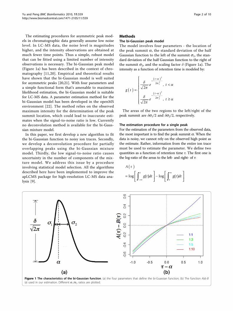
The estimating procedures for asymmetric peak mod-els in chromatographic data generally assume low noiselevel. In LC-MS data, the noise level is magnitudeshigher, and the intensity observations are obtained atmuch fewer time points. Thus a simple, robust modelthat can be fitted using a limited number of intensityobservations is necessary. The bi-Gaussian peak model(Figure 1a) has been described in the context of chro-matography [11,20]. Empirical and theoretical resultshave shown that the bi-Gaussian model is well suitedfor asymmetric peaks [20,21]. With four parameters anda simple functional form that’s amenable to maximumlikelihood estimation, the bi-Gaussian model is suitablefor LC-MS data. A parameter estimation method for thebi-Gaussian model has been developed in the openMSenvironment [22]. The method relies on the observedmaximum intensity for the determination of the peaksummit location, which could lead to inaccurate esti-mates when the signal-to-noise ratio is low. Currentlyno deconvolution method is available for the bi-Gaus-sian mixture model.In this paper, we first develop a new algorithm to fit

the bi-Gaussian function to noisy ion traces. Secondly,we develop a deconvolution procedure for partiallyoverlapping peaks using the bi-Gaussian mixturemodel. Thirdly, the low signal-to-noise ratio causesuncertainty in the number of components of the mix-ture model. We address this issue by a procedureinvolving statistical model selection. All the algorithmsdescribed here have been implemented to improve theapLCMS package for high-resolution LC-MS data ana-lysis [9].

MethodsThe bi-Gaussian peak modelThe model involves four parameters - the location ofthe peak summit a, the standard deviation of the halfGaussian function to the left of the summit s1, the stan-dard deviation of the half Gaussian function to the right ofthe summit s2, and the scaling factor δ (Figure 1a). Theintensity as a function of retention time is modeled by:

g te t

e t

t

t( ) =

<

≥

⎧

⎨

⎪⎪⎪

⎩

⎪⎪⎪

−−( )

−−( )

2

2

2

12

2

22

2

2

,

,

The areas of the two regions to the left/right of thepeak summit are δs1/2 and δs2/2, respectively.

The estimation procedure for a single peakFor the estimation of the parameters from the observed data,the most important is to find the peak summit a. When thedata is noisy, we cannot rely on the observed high point asthe estimate. Rather, information from the entire ion tracemust be used to estimate the parameter. We define twoquantities as a function of retention time τ. The first one isthe log-ratio of the areas to the left- and right- of τ:

A

g t dt g t dt

( )

=⎡

⎣⎢

⎤

⎦⎥ −

⎡

⎣⎢

⎤

⎦⎥

−∞

∞

∫ ∫log ( ) log ( )

Figure 1 The characteristics of the bi-Gaussian function. (a) the four parameters that define the bi-Guassian function; (b) The function A(τ)-B(τ) used in our estimation. Different s1/s2 ratios are plotted.

Yu and Peng BMC Bioinformatics 2010, 11:559http://www.biomedcentral.com/1471-2105/11/559

Page 2 of 10

The second quantity is the log-ratio of the cube-rootof the non-centered second moments of the left- andright- truncated portions of the function:

B

g t t dt

g t t dt

( )

= −( )⎛

⎝⎜

⎞

⎠⎟

− −( )⎛

⎝⎜

⎞

⎠

−∞

∞

∫∫

13

13

2

2

log ( )

log ( ) ⎟⎟

When τ = a, the quantity A(a) is the log ratiobetween the areas of the two half Guassian functions,which is equal to the log ratio between the two standarddeviations; B(a) is the log ratio between the cubic rootsof the variances of the two Gaussian functions multi-plied by their scaling factors, which is also equal to thelog ratio between the two standard deviations. Thus τ =a is a root for A(τ)-B(τ) = 0.

A

( )= ( ) − ( )

=⎛

⎝⎜⎜

⎞

⎠⎟⎟ −

⎛

⎝⎜⎜

log log

log log

1 2

13

23

2 2

13 2

13 2

⎞⎞

⎠⎟⎟

= ( )B

Simulations using a reasonable range of s1/s2 showedthat A(τ)-B(τ) is a monotone function (Figure 1b), whichindicates the solution is unique.In LC-MS data, the intensity values {x1,x2, ..., xn} are

collected at discrete time points {t1,t2, ..., tn}, whichmeans the function g(t) is approximated by a step func-tion. We first define the step sizes of the function:

Δt

t t i

t t i n

t t i ni i i

n n

=− =

−( ) < <− =

⎧⎨⎪

⎩⎪

+ −

−

2 1

1 1

1

1

2 1

,

,

,

We approximate A(τ) by

ˆ

log log

A

x t x ti i

t

i i

ti i

( )

=⎡

⎣

⎢⎢

⎤

⎦

⎥⎥

−⎡

⎣

⎢⎢

⎤

⎦

⎥⎥

< ≥∑ ∑Δ Δ

And B(τ) by

ˆ

log

log

B

x t t

x t t

i i i

t

i i i

t

i

i

( )

= −( )⎡

⎣

⎢⎢

⎤

⎦

⎥⎥

− −( )

<

≥

∑13

13

2

2

Δ

Δ∑∑⎡

⎣

⎢⎢

⎤

⎦

⎥⎥

Because the data are generated from discrete time

points, we first find ˆ ˆA B ( ) − ( ) for all the middle

points between adjacent t’s. Then we interpolatebetween the largest point below zero and the smallestpoint above zero to find ̂ . After finding ̂ , estimating

s1 and/s2 becomes straight-forward:

ˆ ˆ

ˆ ˆ

ˆ ˆ

ˆ

12

22

= −( )

= −( )< <

≥

∑ ∑

∑

t x t x t

t x t x

i i i

t

i i

t

i i i

t

i i

i

Δ Δ

Δ ii i

t

t

i

Δ≥

∑̂

To estimate the scaling factor δ, we first find the fittedvalues without scaling:

ˆ, ˆ

, ˆ

ˆ

ˆ

ˆ

ˆ

ze t

e t

i

t

i

t

i

i

i

=<

≥

⎧

⎨

⎪⎪

−−( )

−−( )

12

12

2

12

2

22

2

2

⎪⎪

⎩

⎪⎪⎪

Then the estimate ̂ is found by a weighted average

of the ratio between the observed intensities and thefitted values without scaling. Because ion counts arehighly skewed, the calculation is carried out in log scale,giving higher weights to points closer to the summit ofthe curve,

ˆˆ log ˆ ˆ

=× ( )∑ ∑

ez x z zi i i

ii

i

2 2

Fitting the bi-Gaussian mixture modelIn LC-MS data from complex samples, e.g. serum orurine, sometimes peaks sharing m/z value may alsopartially overlap in the retention time dimension. Herewe propose an EM-like iterative algorithm to fitpartially overlapping asymmetric peaks. The expecta-tion-maximization (EM) algorithm finds maximumlikelihood estimates of parameters in the presence oflatent variables. It iterates between finding the expecta-tion of the log-likelihood with regard to the latentvariables given the current estimate of the parameters,and finding the parameters that maximize the likeli-hood [23]. In our application, the parameter estimationis not obtained using the maximum likelihood proce-dure, and an extra step of eliminating components thatexplain too small a proportion of the data is added todeal with the noise.

Yu and Peng BMC Bioinformatics 2010, 11:559http://www.biomedcentral.com/1471-2105/11/559

Page 3 of 10

(1) Fit a kernel smoother to the data {(ti,xi)}. Splitthe data points into groups at the valleys of thesmoother. For every group j of the data points, usethe smoother peak as the initial estimate of peak

summit ̂ j , and estimate ˆ , j 1 , ˆ , j 2 , and ̂ j using

the procedure in the previous sub-section. More dis-cussion about smoother parameter selection is pre-sented in the next sub-section.(2) Iterate until convergence:

(2.1) Find the fitted values at every ti for com-ponent j,

ˆ

ˆ, ˆ

ˆ

ˆ

ˆ

ˆ

ˆ

,

,

ze t

e

ij

j

t

i j

j

t

i j

j

i j

j

=<

−−( )

−−( )

2

2

2

12

2

2

2

2

22

, ˆ

, ,

t

i j

i j≥

∀

⎧

⎨

⎪⎪⎪

⎩

⎪⎪⎪

(2.2) For every component j, find the proportionof data explained by the component:

Q

z

zj

ij

i

ik

ik

=∑∑∑

ˆ

ˆ

Remove component j if Qj is smaller than a threshold.

(2.3) For every time point, we find the expectedproportion of the observed intensities that belongto each component j, denoted qij.

qz

zi jij

ij

ik

k

= ∀∑

ˆ

ˆ, ,

Then for every component j, re-estimate

ˆ , ˆ , ˆ , ˆ, , j j j j1 2{ } from the data {(ti,xiqij)}, using the

procedure described in the previous sub-section.

Choosing the number of components of the mixture bystatistical model selectionIn the previous sub-section, the kernel smoother isemployed to obtain an initial estimate of the number ofcomponents and the parameters. When the data isnoisy, changing the window size of the kernel smoothercould result in different numbers of components of themixture. To find the best model to explain the data, weutilize statistical model selection based on the Bayesianinformation criterion (BIC) [24]. BIC is one of the most

popular criteria for the selection among a set of para-metric models with different number of parameters. Itpenalizes the number of free parameters. The modelwith lower BIC value is preferred.First, a reasonable range of the window-size parameter

is determined based on biological/chemical considera-tions about potential peak width. It can be quite lenientto cover a wide range of potential values. Several win-dow size values spanning the range are selected. Startingfrom each of the window-size value, we compute thekernel smoother, and run the EM-like algorithmdescribed in the previous sub-section. The correspond-ing BIC value is computed by:

N x z N

J N

i ij

ji

× −⎛

⎝

⎜⎜

⎞

⎠

⎟⎟

⎛

⎝

⎜⎜⎜

⎞

⎠

⎟⎟⎟

⎡

⎣

⎢⎢⎢

⎤

⎦

⎥⎥⎥

+ × × ( )

∑∑log

log

^

2

4

where N is the total number of time points withobserved intensities, and J is the number of bi-Gaussiancomponents in the model. The model with the lowestBIC value is selected. In the setting of LC-MS data, thisis a heuristic criterion, because the data we observe arenot random samples, and the Gaussian error assumptionof BIC may not be satisfied. We justify the usage of thecriterion by extensive simulations.

SimulationsTo assess the performance of the proposed method,extensive simulations were conducted. The bi-Gaussianmixture model with BIC model selection was comparedwith two other methods - the Gaussian mixture model[9] with BIC model selection, and the peak quantifica-tion based on kernel smoother and signal summation.The data were generated from a 3-component bi-

Gaussian mixture model, with different levels of peakasymmetry, noise and peak overlap. Given the parameters(Additional file 1: Table S1), the data from each compo-nent are generated from the bi-Gaussian functions:

g te t

e t

j

j

t

j

j

t

j

j

j

j

j

( ) =<

≥

⎧

⎨

−−( )

−−( )

2

2

2

12

2

22

2

2

,

,

,

,

⎪⎪⎪⎪

⎩

⎪⎪⎪

After summing the intensities from the components,multiplicative noise was added to the data. In addition, aportion of the values were turned into zero to mimic thebehavior of real high-resolution LC-MS data:

Yu and Peng BMC Bioinformatics 2010, 11:559http://www.biomedcentral.com/1471-2105/11/559

Page 4 of 10

x g t e u

N

u binom

i j i

j

i

i

i

i= ( ) × ×

( )( )

∑

,

~ , ,

~

0

The parameter ξ is the standard deviation of the noiseadded at the log-scale. Three levels of ξ were used inthe simulations (0.2, 0.4, 0.6). At the high noise level ofξ = 0.6, 50% of the intensity values were changed by 1.5fold or more, and 25% were changed by two fold ormore. The parameter θ controls the percentage of valuesturned into zero using random samples from the bino-mial distribution. Three levels of θ were used (0, 0.25,0.5). The value of θ directly corresponds to the propor-tion of intensities turned into zero. In addition, variouslevels of peak asymmetry and overlap were considered(Additional file 1: Table S1). In total 864 parametercombinations were tested. At each parameter setting,the simulation was performed 100 times. For detailedinformation, please refer to Additional file 1.

ResultsSimulation resultsFirst, we compared the rate of successfully selecting thecorrect number of components between the bi-Gaussianmixture model and the Gaussian mixture model(Figure 2). The method of kernel smoother combinedwith signal summation wasn’t compared because no BICmodel selection could be performed using this method,which is a shortcoming in itself. In summarizing theresults, the level of peak overlap is defined by the ratio rbetween the lowest point of the valley between two peaksand the lower of the peak summits, before noise is intro-duced. Because two valleys exist between the three simu-lated peaks, the larger r value is taken for each simulationsetting. For the purpose of plotting, we roughly divide theamount of overlap into four categories: little overlap (r <0.2), moderate overlap (0.2 ≤ r < 0.5), strong overlap (0.5≤ r < 0.75), and severe overlap (r ≥ 0.75). The level ofoverlapping is color-coded. The point size corresponds tothe three levels of noise added to the data (ξ = 0.2,0.4,0.6). The fill of the point represents the proportion ofmissing values (0%, 25% and 50%).When the peaks were symmetric (Figure 2, upper-left

panel), the Gaussian mixture model showed a slightadvantage when the overlapping was strong (red andmagenta points). When the peaks were asymmetric(Figure 2, upper-right and lower-left panels), the bi-Gaussian mixture model showed a clear advantage.When the peak overlapping was not strong (blue andgreen points), the success rate of the bi-Gaussian mix-ture model was mostly higher than 90%, even when the

noise level was high. When there was strong peak over-lapping and the noise level was high (larger sized redand magenta points), the rate of successfully selectingthe correct number of components was reduced forboth the bi-Gaussian mixture model and the Gaussianmixture model.Secondly, we compared the percentage error in peak

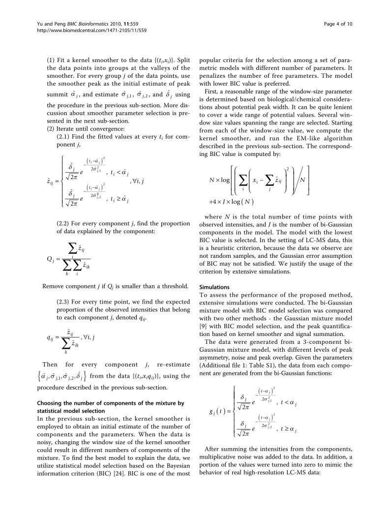
area quantification between the three methods, when allthree methods were able to identify the correct numberof components (not necessarily the best BIC value).Compared to the Gaussian mixture model, the bi-Gaussian mixture model yielded much smaller errorswhen the peaks were asymmetric (Figure 3, upper-rightand lower-left panels). Compared to the method ofkernel smoother combined with signal summation, thebi-Gaussian mixture model showed a clear advantagewhen some of the intensity values were missing (filledpoints) (Figure 4). When the peak overlapping was notstrong (blue and green points), the error of the bi-Gaussian mixture model was mostly under 15%. Furthercomparisons on peak location and peak spread estima-tion are presented in Additional file 1. The bi-Gaussianmixture model also clearly out-performed the other twomethods in those aspects (Additional file 1: Fig. S2~S4).

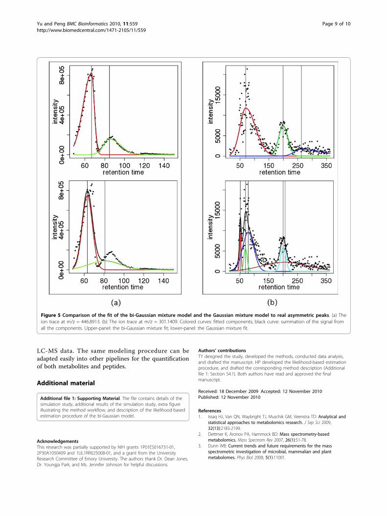
Analysis of high-resolution LC-MS dataWe implemented the new algorithms in the apLCMSpackage for LC-MS metabolomics data analysis [9].When analyzing the example dataset at the apLCMSwebsite, which contains 8 high-resolution LC-MS pro-files, we observed many examples where the peaks wereclearly asymmetric. We show two examples in Figure 5,where both peak asymmetry and peak overlapping exist.In both examples, the inability of the Gaussian curve tofit asymmetric peaks left residuals to be fitted by thesmaller peaks, which caused the smaller fitted peaks todeviate from the local peak shape (Figure 5, lowerpanels). Clearly the bi-Gaussian mixture model fittedthe data much better (Figure 5, upper panels).At the global level, in 21.0% of the ion traces, the bi-

Gaussian mixture model and the Gaussian mixturemodel selected different number of components. Amongthese cases, the bi-Gaussian mixture model fitted thedata with smaller number of components 93.7% of thetime. In addition, it achieved better BIC scores in 66.2%of the cases. Overall, in 59.4% of all the ion traces, thebi-Gaussian (mixture) model achieved better BIC valuescompared to the Gaussian (mixture) model. Consideringthe bi-Gaussian model is penalized more heavily by BICwith the extra parameter, which puts it in disadvantagewhen the peak is close to symmetric, these results indi-cate that the bi-Gaussian peak model is indeed bettersuited for the data.

Yu and Peng BMC Bioinformatics 2010, 11:559http://www.biomedcentral.com/1471-2105/11/559

Page 5 of 10

DiscussionsCompared to the Gaussian peak shape model, which hasbeen used in some model-based data processing pipe-lines [8,9], the bi-Gaussian model provides extra flexibil-ity to fit asymmetric peaks, while suffering littledisadvantage when the true peak shape is symmetric.Compared to the method of kernel smoother combined

with signal summation, fitting a bi-Gaussian mixturemodel disentangles partially overlapping peaks,and copes with the issue of missing intensities in high-resolution LC-FTMS data much better. The bi-Gaussianmodel is among many asymmetric peak models in chro-matographic peak modeling. A large number of othermodels could potentially be used for the processing of

Figure 2 Comparison of the rate of successfully selecting the correct number of components between the bi-Gaussian mixture modeland the Gaussian mixture model. Each sub-plot corresponds to a different degree of asymmetry, as shown in the titles of the sub-plots (ratiosbetween the right- and left- standard deviations). Each dot represents a simulated situation. The values were obtained by averaging the resultsfrom 100 simulations. The color represents the level of overlaps between the simulated peaks. The size of the dot represents the amount ofnoise added to the data. The fill of the dot represents the percentage of values missing in the ion trace.

Yu and Peng BMC Bioinformatics 2010, 11:559http://www.biomedcentral.com/1471-2105/11/559

Page 6 of 10

LC-MS data [11]. Advanced deconvolution methodsalready exist for a few of the models [12-17,19]. How-ever, modifications to the existing estimation proceduresmay be necessary to suit the characteristics of LC-MSdata, i.e. sparser data points and much higher noise.In this study, the parameter estimation for a single

peak is done by numerically solving an equation thatinvolves the zero and second moments of the truncated

distribution functions. An alternative route is touse the maximum likelihood method. We developed alikelihood-based algorithm (Additional file 1: Section S4)and compared its performance with the moment-basedmethod in simulations. The likelihood-based algorithmwas slower in computation due to its iterative nature,and it didn’t achieve better estimation accuracy over themoment-based method. Under the settings of our

Figure 3 Comparison of the accuracy in peak size quantification between the bi-Gaussian mixture model and the Gaussian mixturemodel. Each sub-plot corresponds to a different degree of asymmetry, as shown in the titles of the sub-plots (ratios between the right- andleft- standard deviations). Each dot represents a simulated situation. The values were obtained by averaging the results from 100 simulations. Thecolor represents the level of overlaps between the simulated peaks. The size of the dot represents the amount of noise added to the data. Thefill of the dot represents the percentage of values missing in the ion trace.

Yu and Peng BMC Bioinformatics 2010, 11:559http://www.biomedcentral.com/1471-2105/11/559

Page 7 of 10

simulations, five window size values were used for theinitiation of the model selection process. With bothmethods programmed in R, using a single core of a2.26 GHz Xeon CPU, the median CPU time for solvingthe three-component mixture was 0.15 second forthe moment-based method, and 0.33 second for thelikelihood-based method.

ConclusionIn this manuscript, we presented a method to fit the bi-Gaussian curve to noisy LC-MS ion traces, as well as anEM-like algorithm paired with BIC model selection forthe deconvolution of partially overlapping peaks. Cur-rently, the methods were implemented in the apLCMSpackage for the pre-processing of high-resolution

Figure 4 Comparison of the accuracy in peak size quantification between the bi-Gaussian mixture model and the method of kernelsmoother combined with signal summation. Each sub-plot corresponds to a different degree of asymmetry, as shown in the titles of thesub-plots (ratios between the right- and left- standard deviations). Each dot represents a simulated situation. The values were obtained byaveraging the results from 100 simulations. The color represents the level of overlaps between the simulated peaks. The size of the dotrepresents the amount of noise added to the data. The fill of the dot represents the percentage of values missing in the ion trace.

Yu and Peng BMC Bioinformatics 2010, 11:559http://www.biomedcentral.com/1471-2105/11/559

Page 8 of 10

LC-MS data. The same modeling procedure can beadapted easily into other pipelines for the quantificationof both metabolites and peptides.

Additional material

Additional file 1: Supporting Material. The file contains details of thesimulation study, additional results of the simulation study, extra figureillustrating the method workflow, and description of the likelihood-basedestimation procedure of the bi-Gaussian model.

AcknowledgementsThis research was partially supported by NIH grants 1P01ES016731-01,2P30A1050409 and 1UL1RR025008-01, and a grant from the UniversityResearch Committee of Emory University. The authors thank Dr. Dean Jones,Dr. Youngja Park, and Ms. Jennifer Johnson for helpful discussions.

Authors’ contributionsTY designed the study, developed the methods, conducted data analysis,and drafted the manuscript. HP developed the likelihood-based estimationprocedure, and drafted the corresponding method description (Additionalfile 1: Section S4.1). Both authors have read and approved the finalmanuscript.

Received: 18 December 2009 Accepted: 12 November 2010Published: 12 November 2010

References1. Issaq HJ, Van QN, Waybright TJ, Muschik GM, Veenstra TD: Analytical and

statistical approaches to metabolomics research. J Sep Sci 2009,32(13):2183-2199.

2. Dettmer K, Aronov PA, Hammock BD: Mass spectrometry-basedmetabolomics. Mass Spectrom Rev 2007, 26(1):51-78.

3. Dunn WB: Current trends and future requirements for the massspectrometric investigation of microbial, mammalian and plantmetabolomes. Phys Biol 2008, 5(1):11001.

Figure 5 Comparison of the fit of the bi-Gaussian mixture model and the Gaussian mixture model to real asymmetric peaks. (a) Theion trace at m/z = 446.8913. (b) The ion trace at m/z = 301.1409. Colored curves: fitted components; black curve: summation of the signal fromall the components. Upper-panel: the bi-Gaussian mixture fit; lower-panel: the Gaussian mixture fit.

Yu and Peng BMC Bioinformatics 2010, 11:559http://www.biomedcentral.com/1471-2105/11/559

Page 9 of 10

4. Griffin JL, Kauppinen RA: A metabolomics perspective of human braintumours. Febs J 2007, 274(5):1132-1139.

5. Chen G, Pramanik BN: Application of LC/MS to proteomics studies:current status and future prospects. Drug Discov Today 2009, 14(9-10):465-471.

6. Ahmed FE: Utility of mass spectrometry for proteome analysis: part II.Ion-activation methods, statistics, bioinformatics and annotation. ExpertRev Proteomics 2009, 6(2):171-197.

7. Katajamaa M, Oresic M: Data processing for mass spectrometry-basedmetabolomics. J Chromatogr A 2007, 1158(1-2):318-328.

8. Smith CA, Want EJ, O’Maille G, Abagyan R, Siuzdak G: XCMS: processingmass spectrometry data for metabolite profiling using nonlinear peakalignment, matching, and identification. Anal Chem 2006, 78(3):779-787.

9. Yu T, Park Y, Johnson JM, Jones DP: apLCMS–adaptive processing of high-resolution LC/MS data. Bioinformatics 2009, 25(15):1930-1936.

10. Ahmed FE: Utility of mass spectrometry for proteome analysis: part I.Conceptual and experimental approaches. Expert Rev Proteomics 2008,5(6):841-864.

11. Di Marco VB, Bombi GG: Mathematical functions for the representation ofchromatographic peaks. J Chromatogr A 2001, 931(1-2):1-30.

12. Felinger A: Deconvolution of Overlapping Skewed Peaks. AnalyticalChemistry 1994, 66(19):3066-3072.

13. Johansson M, Berglund M, Baxter DC: Improving Accuracy in theQuantitation of Overlapping, Asymmetric, Chromatographic Peaks byDeconvolution - Theory and Application to Coupled Gas-Chromatography Atomic-Absorption Spectrometry. Spectrochim Acta B1993, 48(11):1393-1409.

14. Papai Z, Pap TL: Determination of chromatographic peak parameters bynon-linear curve fitting using statistical moments. Analyst 2002,127(4):494-498.

15. Youn DY, Yun SJ, Jung KH: Improved Algorithm for Resolution ofOverlapped Asymmetric Chromatographic Peaks. J Chromatogr 1992,591(1-2):19-29.

16. TorresLapasio JR, GarciaAlvarezCoque MC, BaezaBaeza JJ: Global treatmentof chromatographic data with MICHROM. Anal Chim Acta 1997, 348(1-3):187-196.

17. Caballero RD, Garcia-Alvarez-Coque MC, Baeza-Baeza JJ: Parabolic-Lorentzian modified Gaussian model for describing and deconvolvingchromatographic peaks. Journal of Chromatography A 2002, 954(1-2):59-76.

18. Powell MJD: A Method for Minimizing a Sum of Squares of Non-LinearFunctions without Calculating Derivatives. Comput J 1965, 7(4):303-307.

19. TorresLapasio JR, BaezaBaeza JJ, GarciaAlvarezCoque MC: A model for thedescription, simulation, and deconvolution of skewed chromatographicpeaks. Analytical Chemistry 1997, 69(18):3822-3831.

20. Buys TS, De Clerk K: Bi-Gaussian fitting of skewed peaks. AnalyticalChemistry 1972, 44(7):1273-1275.

21. Felinger A: Data Analysis and Signal Processing in Chromatography.Amsterdam: Elsevier Science;, 1 1998.

22. Sturm M, Bertsch A, Gropl C, Hildebrandt A, Hussong R, Lange E, Pfeifer N,Schulz-Trieglaff O, Zerck A, Reinert K, et al: OpenMS - an open-sourcesoftware framework for mass spectrometry. BMC Bioinformatics 2008,9:163.

23. Dempster AP, Laird NM, Rubin DB: Maximum Likelihood from IncompleteData Via Em Algorithm. J Roy Stat Soc B Met 1977, 39(1):1-38.

24. Schwarz G: Estimating Dimension of a Model. Ann Stat 1978, 6(2):461-464.

doi:10.1186/1471-2105-11-559Cite this article as: Yu and Peng: Quantification and deconvolution ofasymmetric LC-MS peaks using the bi-Gaussian mixture model andstatistical model selection. BMC Bioinformatics 2010 11:559.

Submit your next manuscript to BioMed Centraland take full advantage of:

• Convenient online submission

• Thorough peer review

• No space constraints or color figure charges

• Immediate publication on acceptance

• Inclusion in PubMed, CAS, Scopus and Google Scholar

• Research which is freely available for redistribution

Submit your manuscript at www.biomedcentral.com/submit

Yu and Peng BMC Bioinformatics 2010, 11:559http://www.biomedcentral.com/1471-2105/11/559

Page 10 of 10