Quality, Upgrades and Equilibrium in a Dynamic

Monopoly Market

James J. Anton and Gary Biglaiser�

12 March, 2012

Abstract

We examine an in�nite horizon model of quality growth for a durable goods

monopoly. Quality improvements may be sold in any desired bundles. Consumers

are identical and for a quality improvement to have value the buyer must possess

previous qualities: goods are upgrades. Subgame perfect equilibrium seller payo¤s

range from capturing the full social surplus down to only the initial �ow value of

each good, as long as the value of all future quality growth exceeds the value of

a single unit. Each of these payo¤s is realized in a Markov perfect equilibrium

that follows the socially e¢ cient path. However, ine¢ cient delay equilibria, with

bundling, exist for innovation rates above a threshold.

JEL: C72, C73, D42, L15

Keywords: Upgrades, durable goods, monopoly, market power, coordination

We examine the commercialization process - pricing and adoption - of an upgrade good

in a dynamic monopoly market. Prominent examples are provided by technology markets,

such as those for software, where cycles of upgrades to existing products have become the

�Anton: Fuqua School of Business, Duke University, Durham NC 27705, james.anton@duke.edu;Biglaiser: Department of Economics, University of North Carolina, Chapel Hill NC 27599,gbiglais@email.unc.edu. We are grateful to the Fuqua Business Associates Fund and Microsoft for �-nancial support. We thank Harvard Business School, the Portuguese Competition Authority, and UCSDfor their hospitality where some of this research was conducted. We also thank the associate editorand referees, as well as Jacques Cremer, Leslie Marx, Larry Samuelson, Jean Tirole, Mike Waldman,Dennis Yao, many colleagues at conferences and seminars, and, especially, Joel Sobel for many helpfulconversations. The views in this work are solely are own.

1

norm.1 Ongoing innovation implies that buyers face a sequence of purchasing decisions.

Thus, rather than timing a single purchase and then exiting the market, buyers have an

incentive to return to the market and �upgrade�to a higher quality. Buyer expectations

are pivotal for these decisions and, given the recurrent aspect of upgrading, bundling by

the seller emerges as a critical aspect of the upgrade o¤ers.

The Microsoft antitrust cases highlight a fundamental question regarding prices in

an upgrade market. Fudenberg and Tirole (2000) observed that the expert witnesses all

appeared to agree that Microsoft was pricing the Windows operating system well below

the static monopoly price. There was, however, wide disagreement as to why. Prominent

arguments included network formation with low prices spurring adoption, limit pricing

where a low price deters rivals, and leverage to gain sales in markets for application

programs. Implicit in all of these arguments is the presumption that prices would be

higher in the absence of these forces. There is, however, no model of dynamic monopoly

that provides a basis for this claim. We provide a game theoretic analysis of dynamic

monopoly pricing for an upgrade good and establish that, in equilibrium, high prices are

not a necessary outcome. Signi�cantly, low prices, as measured by a seller who captures

a small share of the social surplus, emerge in equilibrium.

Upgrade markets, by de�nition, regularly confront buyers with the choice of adopting

a new higher-quality version or remaining with their current version. Microsoft�s recent

introduction of Vista was an adoption failure as buyers overwhelmingly chose to stay with

their existing XP version, echoing a previous episode with Windows Millennium in 2000.

Microsoft moved quickly to introduce a new version. Windows 7 was launched in late

October 2009 to a much more favorable buyer response. As early as May 2009, Microsoft

CEO Steve Ballmer acknowledged that �If people want to wait [for Windows 7], they

certainly can.�This simple observation, which implicitly takes the failure of Vista as a

given, leads to a more subtle set of questions.

Consider the initial o¤er of Vista. An individual buyer has the option of remaining

with XP. If most other buyers had purchased Vista then we can expect a concern about

�falling behind� the market to be pivotal for an individual buyer�s willingness to pay.

Given that others did not purchase Vista, an individual buyer who stayed with XP is

in the position Ballmer described. By purchasing Vista a buyer would �jump ahead�of

1Quality improvement is important in durable goods markets, as emphasized by Waldman (2003). Inaddition to software, upgrades to cellular networks often allow vendors to o¤er, for an added charge, newor improved services such as web browsing, e-mail access and text messaging. Many capital goods areregularly upgraded, including airports (terminals and runways) and oil re�neries, among others.

2

the market and then be confronted with the choice of purchasing Windows 7 to �keep

up�with market, assuming that Windows 7 is widely adopted. How does this recurrent

interplay of individual and collective decisions with respect to incentives to �fall behind�

or �jump ahead� of the market work to determine prices and adoption in an upgrade

market? We argue that the ability of the seller to tempt an individual buyer to �jump

ahead�is the critical factor and that this incentive provides the basis for a credible threat

to reject an upgrade o¤er. Moreover, low prices can emerge even when buyers have a very

strong incentive not to �fall behind�the market.

Our in�nite horizon model of an upgrade market has a very simple economic structure.

Innovation is exogenous but ongoing and in each period it is feasible for the seller to o¤er

an additional quality increment. Buyers are homogeneous and have a �xed valuation per

unit of quality; this corresponds to a horizontal demand curve in a static setting. Building

on the recent literature, we assume �upgrade�goods satisfy a downward complementarity

property: an additional quality increment is valuable only if a buyer holds all previous

quality increments. The seller is unconstrained with respect to bundling options and any

combination of quality increments (a single bundle or a set of bundles) may be o¤ered in

each period. Bundling is thus endogenous.

This basic structure is arguably a very attractive setting for the seller - homogenous

buyers with a �xed valuation per quality unit, unrestricted bundling, and a costless exoge-

nous �ow of upgrade innovations. It is natural to expect a �perfect�monopoly outcome

in which the seller captures all of the social surplus, and this is exactly what happens

in several benchmark cases. For example, when the seller can only o¤er a single good

of �xed quality and buyers are homogeneous, the seller can make an o¤er that induces

buyers to purchase now. This �speed-up� argument, for which an elegant version was

developed by Fudenberg, Levine, and Tirole (1985) for a sequential o¤er game, is quite

powerful and it undermines the credibility of buyers to reject o¤ers with high prices.2 In

sharp contrast, we �nd that surplus growth due to rising quality in an upgrade market

provides buyers with an option to return to the market for future purchases, rather than

exiting permanently after a single purchase, and that this option leads each buyer in a

2The standard incentive (Coase (1972)) to cut price over time and move down the demand curve is notpresent with identical buyers. Papers on the Coase conjecture with a single good and heterogeneous buyersinclude Stokey (1981), Bulow (1982), and Gul, Sonnenschein, and Wilson (1986). Ausubel and Deneckere(1989), Fehr and Kuhn (1995) and Sobel (1991) provide folk theorems. Bond and Samuelson (1984)examine a rational expectations equilibrium with depreciation and replacement sales. Methodologically,we are closest to Sobel (1991). In both cases, the market never closes, due to new demand in the case ofSobel and to quality growth in our case.

3

group to reject an o¤er that a single buyer would not.

The primary intuition is as follows. Suppose that buyers expect to receive a positive

share of the surplus on future quality improvements. Further, imagine that the seller o¤ers

a price above the candidate equilibrium for today�s upgrade. Is it credible for buyers to

refuse the o¤er? Consider the willingness to pay of an individual buyer when other buyers

are expected to refuse the o¤er. When others refuse, we have delay and the next period

will have the larger surplus due to quality growth and a market state in which buyers

lack the previous upgrade. When the typical buyer�s share of this surplus is signi�cant,

a solitary individual buyer who purchased the high priced upgrade in the last period will

wish to purchase again; while this may require the buyer to �re-purchase�some quality

increments, the signi�cant buyer share of future surplus makes it attractive to keep up

with the market. But, then the initial upgrade purchase of a buyer who �jumps ahead�of

the market reduces to a one-period �ow of value. As a result, willingness to pay is limited

to the one-period �ow value. We can apply this result at any stage of the game provided

only that the surplus generated by all future upgrades exceeds the surplus of one unit.

The credible threat to reject a seller o¤er, given that other buyers also reject, leads to an

implicit form of coordination among buyers and, in turn, to multiple equilibria.

We construct Markov perfect equilibria for this dynamic game. Two classes of equilib-

ria are identi�ed: e¢ cient and generational. E¢ cient equilibria have buyers acquiring a

new upgrade each period and payo¤s span a signi�cant economic range. At one extreme,

the seller captures all surplus and each quality increment sells immediately for the full

present discounted value. At the other extreme, each increment sells only for the one

period �ow value, leaving a buyer with the entire residual surplus. This is the range of

subgame perfect payo¤s and each is realized in a Markov perfect equilibrium.

In contrast, and despite the complete information setting, ine¢ cient equilibria do exist.

These �generational�equilibria exhibit cyclical delay in which multiple quality increments

go unsold until they are bundled together for sale and, necessarily, the market returns to

the �state of the art�with a new generation. The cycle length re�ects a second type of

equilibrium coordination in an upgrade market. Importantly, relative to the set of e¢ cient

equilibria, we �nd that generational equilibria compress the range of payo¤s. Intuitively,

delay requires that deviations to make early trades are unattractive, and this implies that

the seller and the buyers share the joint surplus more equally.

The seller is free to o¤er any feasible collection of quality units. On the equilibrium

path, it is su¢ cient to consider only upgrade o¤ers with a contiguous set of quality units.

4

Equivalently, we show how to interpret these upgrade o¤ers in terms of a full bundle (new

version of the product) with pricing contingent on a buyer�s current product holding,

much as the owner of an existing product faces an upgrade price to acquire a new version.

Furthermore, we �nd no role for the commitment period (time between seller o¤ers),

in contrast to the literature on the Coase Conjecture. What matters for equilibrium

outcomes is the frequency at which quality improves: allowing the seller to make o¤ers

more frequently has no impact with homogenous buyers.

There is a relatively small literature on upgrade models, with most of the work involv-

ing a �nite horizon. Waldman (1996) and Nahm (2004) each examine a two period model,

focusing on the incentive to invest in quality growth and R&D time inconsistency. Fuden-

berg and Tirole (1998) examine a two-period model where consumers are heterogeneous

and the period two (new) good renders the period one (old) good obsolete; Hoppe and Lee

(2003) extend this model to allow entry. Ellison and Fudenberg (2000) analyze a series of

static and two period models that feature network externalities and a cost to consumers

of upgrading the good. In the �nite horizon version of our model, the monopolist captures

all surplus, since a credible buyer threat is undermined by the terminal period. Fishman

and Rob (2000) examine an in�nite horizon upgrade model, focusing on innovation incen-

tives, and analyze a rational expectations equilibrium in which the seller is assumed to

o¤er only a single bundle consisting of all prior quality levels. We focus on pricing and

adoption, taking innovation as exogenously given, and provide a game-theoretic analysis

in which the seller choice of which bundles (and prices) to o¤er is endogenous.

In the next section, we present the model. In Section 2 we examine e¢ cient equilibria

and in Section 3 we examine generational equilibria. We discuss the upgrade structure

of our model in Section 4 and consider directions for future research in Section 5. Proofs

are in the Appendix; all omitted proofs are in Anton and Biglaiser (2010b).

1 The Model

We �rst describe the basic elements of the game. We next turn to strategies and

payo¤s, and then de�ne and discuss Markov perfect equilibrium. We present the formal

theoretic framework for bundling (strategies and equilibrium) in Appendix A.

5

1.1 Basic Elements

We examine an in�nite horizon, discrete time model. Let � = 1; 2; ::: index periods.

There is a continuum of identical buyers with a measure of 1 represented by the unit

interval and a single seller. A new perfectly durable good, unit � , becomes available in

each period � . All seller costs are 0: In period � , feasible o¤ers for the seller consist of any

collection of subsets of f1; 2; :::; �g and associated prices. For example, the seller can o¤erthe bundle of all feasible qualities f1; 2; :::; �g for a price p, so that the new unit is madeavailable only as part of a larger bundle. Alternatively, the seller can o¤er a collection of

individual unit bundles, f1g at price p1, quality f2g at a price p2, and so on; a buyer couldpurchase every feasible quality or any subset of the available unit bundles. The seller can

also withhold some qualities or even make no o¤er. Given a seller o¤er, buyers respond

simultaneously with each choosing which bundle(s) to accept in period � .3

An upgrade is a bundle that consists only of a set of contiguous qualities. For example,

a �state of the art upgrade�from a status quo of 0 is the bundle f1; :::; �g; we also refer tothis as a version. A partial upgrade is a bundle f�; :::; � + kg, where 1 � � � � + k � � :

We will show that, in equilibrium, a seller need only make upgrade o¤ers.

A buyer holding contiguous units 1; :::; q but not q + 1 has a �ow utility of vq in a

period. Thus, a buyer must have all lower quality units for quality q to have value. This

�downward complementarity�assumption is the upgrade payo¤ structure in our model.

Players are all risk neutral and have a common discount factor � < 1. Because a new

unit of quality becomes available in each period, the discount factor re�ects the rate of

innovation as well as the rate of time preference for the players. Thus, we can interpret a

large (small) � in terms of rapid (slow) rate of innovation and assess limiting behavior.

Consider the payo¤ for a buyer. In each period, a buyer holds some subset of the

feasible qualities. Let q� denote the maximal contiguous quality held by a buyer after any

purchase in period � . That is, a buyer holds units 1 up through q� but does not hold unit

q� + 1. From any point in the game, the payo¤ of the buyer is the present discounted

value from quality �ows net of payments. From the start of the game this is given by

1X�=1

���1(vq� � p� );

3We do not impose any arbitrage structure across bundles. For example, if the seller o¤ers seperatebundles for units 1 and 2, then there is no restriction on the price of a bundle of units 1 and 2. Rather,buyer choices determine which of these bundles will be purchased. Also, since buyers are identical, thereare no possible gains in equilibrium for buyers from the possibility of resale.

6

where p� is the payment made by the buyer in period � . Similarly, the payo¤ of the

seller from any point onward is the present discounted value of revenues, r� , from sales to

buyers. From the start of the game, this is given by

1X�=1

���1r� :

Consider e¢ cient allocations. Payments and revenues are transfers that do not a¤ect

total surplus. Thus, for any path of quality holdings and payments, the sum of surplus

for any given buyer and the seller from any period � 0 is

1X�=�0

����0vq� :

Thus, the realized joint surplus is fully determined by the quality path. Since q� � � for

any feasible path and q0 � 0, the joint surplus is maximized when each buyer holds themaximal quality, q� = � . The surplus in an e¢ cient allocation from the start is

S1 = v + �2v + �23v + ::: =v

(1� �)2:

Intuitively, S1 is the surplus created when buyers acquire one new unit in each period,

where each new unit has a present discounted value of v1�� : Starting from any period � ;

the maximal available surplus is

S� = v� + �v(� + 1) + �2v(� + 2) + ::: =v(� � 1)1� �

+ S1:

Intuitively, the di¤erence between S� and S�+1 is the �ow value of � units in period � .

Thus, we always have S� > �S�+1, as delay necessarily involves lost surplus and hence

ine¢ ciency. However, because each unit generates surplus, we also have S� < S�+1.

1.2 Markov Perfect Equilibrium

We examine Markov perfect equilibria (MPE) as de�ned by Maskin and Tirole (2001),

with the natural modi�cation for a continuum of agents. By de�nition, Markov strategies

depend only on the payo¤ relevant aspects of a history of the game. In our model, the

seller�s �ow payo¤ depends only on revenues and each buyer�s �ow payo¤ depends only

on the maximal contiguous unit held and the payments in a period. Thus, past prices

7

and the timing of buyer acquisitions do not in�uence current period payo¤s.

The simplest form of Markovian behavior is to focus on the distribution of maximal

contiguous units across buyers and the gap relative to the current period � , which indexes

the seller�s feasible units. This allows us to generate all subgame perfect equilibrium

seller payo¤s. To proceed, consider any history in which all buyers enter period � with

the same maximal quality level Q (units 1 through Q). We de�ne this to be state (� ;Q)

and refer to � � Q as the quality gap. Markovian behavior is de�ned by the condition

that players� strategies depend only on the size of the quality gap. Thus, if the seller

o¤ers an upgrade of � units at a price p in state (� ; 0), then an upgrade from Q to Q+ �

at the same price p must be o¤ered in state (� 0; Q), provided that the gaps coincide,

� 0 �Q = � . Furthermore, except for a translation of the index number on quality units,

buyers�accept/reject decisions are the same in states (� ; 0) and (� 0; Q). This implies that

the seller�s pro�ts and buyers�utilities satisfy

�� � �(� ; 0) = �(� 0; Q);

u(� 0; Q) =vQ

1� �+ u(� ; 0) and u� � u(� ; 0)

for � 0 �Q = � .4 Thus, buyer payo¤s are always the sum of the PDV of current holdings,

vQ=(1 � �); and the incremental utility, u� . When there is no risk of confusion, we will

use � rather than (� ; 0) to refer to the state.

This de�nition of Markovian behavior implies that the same number of units are

included in an upgrade bundle whenever the quality gaps coincide. In particular, the

seller is not required to o¤er the full bundle of all feasible units; we discuss contingent

pricing and versions in section 4. Henceforth, we use equilibrium to refer to a pure strategy

buyer symmetric Markov perfect equilibrium in the quality gap.5

We follow Gul, Sonnenschein, and Wilson (1986), Ausubel and Deneckere (1989), and

Sobel (1991), among others, and restrict attention to equilibria that satisfy a zero-measure

property: for any two histories (past seller o¤ers and buyer acceptances) that di¤er only

with respect to the actions of a set of buyers of measure zero, the strategies of the seller

4Feasible payo¤s have a simple stationary structure. Any subgame perfect equilibrium from state(� + 1�Q; 0) is also subgame perfect from state (� + 1; Q) once we relabel units and translate payo¤s.

5Asymmetric buyer holdings are o¤-the-equilibrium path as are histories with multiple upgrade o¤ers.Mixing by buyers in response to a seller o¤er would lead to asymmetric holdings and this is often neededfor continuation equilibria in the durable goods literature. In our case, because buyers never exit themarket, we are able to construct pure strategy continuation equilibria in all states. The Appendix providesa detailed analysis for any distribution of buyer holdings and for any seller o¤ers.

8

and all other buyers are the same across the two histories. As a result, buyers act as price

takers: no buyer expects that their own decision will have any impact on subsequent play,

such as a¤ecting future seller o¤ers.

Finally, to streamline the equilibrium analysis, we specify strategies such that an in-

dividual buyer who deviates by not following other buyers in a purchase that increases

the maximal buyer quality will obtain no future additional surplus. Thus, if an individual

buyer has the �rst k units of the good, when all other buyers also have additional con-

tiguous units, then this buyer�s continuation payo¤ is vk=(1 � �).6 We can easily allow

for higher buyer catch-up continuation values as long as they do not exceed the equilib-

rium payo¤. For the analysis, however, it is helpful to follow the above speci�cation of a

zero increment in utility for a buyer who falls behind the market. This will highlight the

critical role played by the incentive for a buyer to jump ahead of the market.

2 E¢ cient Equilibria

We begin with a basic result on the necessary structure with respect to all equilibrium

payo¤s: the seller can always induce buyers to make a purchase.

Lemma 1 (Flow Dominance) Consider any history such that, at the start of period � , allbuyers hold the �rst Q quality units and no buyer holds unit Q+1, where � > Q. Suppose

the seller makes an upgrade o¤er for units fQ+ 1; :::; �g at price p, where p < v(� �Q).

Then, in any continuation equilibrium, every buyer accepts the upgrade o¤er.

The intuition for ��ow dominance�is simple. The upgrade from Q to � is priced su¢ -

ciently low that that it pays for itself in the current period, since v� � p > vQ. Moreover,

even if all other buyers were to reject the o¤er, an individual buyer who accepts is always

weakly better o¤ in the future. This follows from (1) the upgrade payo¤ structure, since

an accepting buyer has a �ow surplus of at least v� in future periods, and (2) all buyers

have the same opportunities for purchasing from the seller, so an accepting buyer always

has the option of making the same choices in the future as other buyers.

Lemma 1 implies that in state � the continuation payo¤ of the seller is at least v� +

�v=(1� �). First, the seller can o¤er � units at �ow value. Second, in the future each new6One can interpret this as (i) the seller (optimally) ignores individual buyers (measure zero) who di¤er

from the market path, or (ii) the seller o¤ers the necessary units but the upgrade price extracts all ofthe continuation surplus. By the zero measure property, the seller must either completely refrain frommaking �catch-up�o¤ers, or always make such o¤ers.

9

unit can be sold at v. Lemma 1 and this �ow dominance payo¤ bound are basic results.

They apply to any subgame perfect payo¤ and do not depend on Markovian behavior or

symmetric buyer strategies: they only rely on buyers acting as price takers.

In an e¢ cient equilibrium, a good is sold in each period when it �rst becomes available.

At the start of the game, the seller o¤ers the �rst unit at price p1 and all buyers accept. In

the second period, the state is then (2; 1) and the quality gap is again 1. Under Markovian

behavior, the seller o¤ers the second unit at price p1 and all buyers accept, leading to

state (3; 2); and so on. Thus, the �rm earns a pro�t of �1 = p1=(1� �), buyers receive a

payo¤ of u1 = 11��

�v1�� � p1

�, and they share the maximal social surplus, S1 = �1 + u1.

To highlight the economic forces at work, we next discuss the extremal equilibria. We

then develop su¢ cient conditions and characterize e¢ cient equilibria.

2.1 Equilibria with extreme payo¤s

Consider the two extremal equilibria. In the �rst, the seller captures all of the social

surplus while the buyers receive a payo¤of zero; each new upgrade unit is sold at the price

p1 =v1�� . In the second, the seller payo¤ is held to the one-period �ow value while the

buyers capture the full residual value; each new upgrade unit is sold at the price p1 = v:

Both equilibria follow the e¢ cient path. Furthermore, each is supported by an immediate

return to the e¢ cient path in the event of deviations: in any state � the seller o¤ers a state

of the art bundle, a �cash-in�o¤er so that no feasible units remained unsold, and buyers

choose to accept. Each equilibrium re�ects implicit buyer coordination on the price p1and any higher price o¤er is rejected by all buyers. Thus, it is important to understand

both how the low price equilibrium is supported by a credible (buyer) threat to reject

prices above �ow value and why such a threat is inoperative in the high price equilibrium.

Consider the low price equilibrium and suppose the seller o¤ers an upgrade at a price

above v. If other buyers are expected to reject this o¤er, a buyer who deviates and accepts

also has the option to make future purchases. In the low price equilibrium, the supporting

cash-in o¤er for 2 units has a continuation payo¤ for a buyer who did not purchase last

period that is strictly greater than v1�� . Consequently, the deviating buyer will choose to

accept this o¤er and rejoin the other buyers rather than fall behind for a continuation

payo¤ of v1�� . But this implies the same continuation payo¤ for the deviating buyer and

for buyers who did not purchase last period. Returning to the initial deviation, given that

other buyers are expected to reject, the deviating buyer will pay at most the �ow value of

v for the �rst unit. Hence, the equilibrium coordination of buyer decisions�on the price

10

p1 supports the credible threat to reject higher prices.

We can extend this logic of a credible threat based on buyer coordination to support

the entire range of buyer payo¤s between 0 and �S1 in equilibrium. As suggested by a

willingness to pay equal to the �ow value v in the low price equilibrium, we are able to

construct a credible threat for any discount factor greater than 1=2. Essentially, � > 1=2

is a growth condition on social surplus as it implies that the incremental surplus from

future units is larger than the value of the current unit (�S1 > v1�� ). The future surplus

is then su¢ cient to maintain the incentive of a deviating buyer to rejoin the support path

and thus establish a credible threat to reject price increases.

By contrast, the high price equilibrium is very simple. Since other buyers accept any

price up to v1�� , a deviating buyer who rejects will fall behind the market and receive 0 (by

construction). Thus, an individual buyer will accept any price up to v1�� . This logic does

not rely on surplus growth and the high price equilibrium exists for all discount factors.

Comparing the low and high price equilibria, we see that the incentives of an individual

buyer depend on other buyers�accept/reject decisions, since future seller o¤ers will vary

with the market state. Thus, buyer coordination matters in an upgrade market.

2.2 Su¢ cient Conditions

In an e¢ cient equilibrium, the seller o¤ers the current unit at p1, all buyers accept, and

the market cycles. For these to be optimal actions, we must specify continuation payo¤s

that rule out deviations.7 Suppose that in state � � 2, the seller o¤ers � units at a pricep� and this is accepted by all buyers. We de�ne this to be a �cash-in�support. Thus, the

next state is (� +1; �), where the quality gap has returned to 1. The continuation payo¤s

with this support are �� = p� + ��1 and u� = v�1�� � p� + �u1.

Buyers follow a simple cut-o¤ rule: a buyer accepts the seller o¤er of price p for � units

in state � if and only if p � p(�; �). On the acceptance side, it must be optimal for an

individual buyer to accept any o¤er p � p(�; �), given that all other buyers are accepting

(symmetric strategies) and the quality gap moves to � +1� �. Rejecting when others allaccept yields 0 by construction, as the buyer falls behind the market. Accepting along

with other buyers yields a current �ow of v�� p plus a future value of ��v�1�� + �u�+1��

�.

Thus, it is optimal for all buyers to accept p for � units in state � if v�1�� + �u�+1�� � p.

7We apply the one-stage-deviation principle to verify the proposed strategies constitute an equilibrium;our model conforms to the necessary requirement of �continuity at in�nity,�since the limit of ��� is 0 as� goes to in�nity (see Fudenberg and Tirole (1991) pp. 108-110).

11

This re�ects the incentive of a buyer to �keep up�with the market.

The rejection side of the cut-o¤ rule re�ects the incentive not to �jump ahead�of the

market, and an o¤er of p > p(�; �) must be rejected by all buyers. Rejecting when others

reject yields a payo¤ of �u�+1. More subtly, accepting when all other buyers reject yields

a �ow of v��p plus the option of purchasing the cash-in o¤er for � +1 units next period.Thus, an individual buyer optimally rejects when others reject if

p > v� + �max

�v�

1� �; u�+1

�� �u�+1 � g(�; u�+1):

Intuitively, when the other buyers purchase the cash-in o¤er in state � + 1, a deviating

buyer who accepted in � has two options. If u�+1 > v�1�� , it will be optimal to purchase

with the other buyers. Thus, the deviating buyer is initially willing to pay at most the

�ow value of the units, v�, in state � . Otherwise, the buyer will not purchase in � + 1

and is willing to pay up to v�1�� � �u�+1.

Thus, combining the acceptance and rejection sides of the cut-o¤ strategy we have

g(�; u�+1) � p(�; �) � v�

1� �+ �u�+1�� (1)

for all 0 < � � � and all � � 1. The cut-o¤ strategies apply to full (� = �) and partial

(� < �) cash-in o¤ers. Since g is bounded above by v�1�� , cut-o¤ strategies exist for any

non-negative utility sequence. The lower bound on g of v� re�ects �ow dominance.

The distinct upper and lower bounds on the cut-o¤rule show that an individual buyer�s

willingness to pay depends on the actions of other buyers. It is important to recall that

there are no network externalities in our model, which is a standard reason for why buyers

make their purchasing decisions based on expectations of other buyers�choices. Instead,

the linkage of decisions arises from i) quality growth and the resulting incentive for a buyer

to return to the market for another upgrade, ii) the seller�s o¤er in the future depends

on �the state of the market�and, iii) an individual buyer will be a¤ected by his position

relative to the market when making future purchasing decisions.

Given these buyer cut-o¤ strategies, the seller must �nd it optimal to o¤er � units at

price p� in state � . The seller has three ways of deviating: make no o¤er, a �delay;�o¤er

an upgrade of less than � units, a �partial cash-in;�or o¤er an upgrade of � units but not

at price p� . For partial cash-ins, p(�; �) is the optimal price choice for any such o¤er and

12

it generates a payo¤ of p(�; �) + ���+1��. Then equilibrium requires

�� � ���+1�� � p(�; �) (2)

for � = 1; :::; � � 1. Delay, � = 0, is not optimal if �� � ���+1. De�ning p(0; �) � 0, (2)applies. Finally, for a cash-in o¤er of � units, buyers will accept any price below p(� ; �),

so we must have p� = p(� ; �) or else the seller could successfully o¤er a price above p� .

Note that (2) is an equality at � = � , by equilibrium construction. Similarly, the buyer

condition (1) also applies for delay (� = 0) and on the equilibrium path (� = � = 1).

Combining the price bounds from (1) and (2), we must have

�� � ���+1�� � p(�; �) � g(�; u�+1).

Since S� = �� + u� in an e¢ cient equilibrium, the above condition is equivalent to

S� � �S�+1�� � u� � �u�+1�� + g(�; u�+1), (3)

for 0 � � � � and � � 1: The surplus di¤erence on the left hand side is an increasing,

exogenous sequence in � : as � grows and more units are �on the table,�a larger set of

utilities can be supported.8 Given utilities that satisfy (3), we can clearly construct the

supporting prices p(�; �) for conditions (1) and (2). When (3) holds, the optimal upgrade

o¤er for the seller is to o¤er � units for the price p� . Each buyer then �nds it optimal to

accept the upgrade o¤er, given that all other buyers also accept. We then have

Lemma 2 Suppose the sequence of buyer utilities u� satis�es (3). Then there exists ane¢ cient equilibrium with a buyer payo¤ of u1:

The proof that (3) is su¢ cient for the existence of an equilibrium outcome with payo¤

u1 is by construction. Taking a given u1, the rest of the utility sequence is speci�ed in

the next section. For this sequence, we must show that it is not pro�table for the seller

to deviate by o¤ering multiple upgrade options (as well as options with non-contiguous

units); note that (3) only rules out seller deviations involving a single upgrade o¤er. This

requires that we specify buyer strategies in response to any o¤er from the seller. In

addition, we must specify strategies for continuation equilibria in the event that buyer

holdings are distributed asymmetrically across units even though such events are o¤ the8In the benchmark case of a single good, where a buyer exits the market after a purchase, (3) reduces

to 0 � u1 and all surplus accrues as pro�t.

13

equilibrium path. In all cases, the support returns to the equilibrium path after 1 period.

See Appendix B for the support construction.

2.3 Existence and Payo¤s

The sequence of utilities that we construct to satisfy the su¢ cient condition (3) has

two phases. When the quality gap is T or smaller, the support makes the seller indi¤er-

ent between a cash-in and delay; for larger quality gaps the support keeps buyer utility

constant at uT . Thus, for T � 2 we de�ne a T � stage support utility sequence by

u� =

(v� + �u�+1 for � = 1; :::; T � 1uT for � � T:

(4)

For any given u1 and length T , the sequence (u2; :::; uT ) is determined.

A direct consequence of a T-stage support is that we only to need to satisfy the

support constraints, (3), over the range � = 1; :::; T ; see Lemma A1 in Appendix B. This

is because, when (3) holds at � = T , then it necessarily holds at all larger � whenever

utility remains constant and the seller is the residual claimant of surplus growth. Thus, an

advantage of a T � stage support is that we only have to check a �nite set of conditions.We now turn to �nding the appropriate length for the T � stage support.

Consider any given u1 2 [0; �S1], and then de�ne T by (1��T�1)S1 < u1 � (1��T )S1.For each u1, this condition de�nes a unique T � 1, since � � 1��T holds for T su¢ cientlylarge. Thus, higher buyer payo¤s require a larger T . We see from (4) that for � � T

u� =

T�1Xs=�

vs�s�� + �T��uT :

Setting � = 1, the given u1 together with the speci�ed T yield uT , as required. From uT

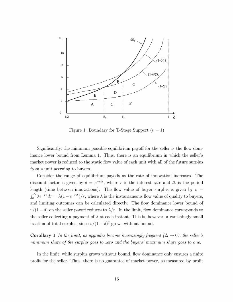
and T , the other utility values follow directly by taking � = 2; :::; T � 1.Figure 1 then illustrates the relationship between u1 and T for the range of � 2 [1=2; 1].

De�ne a set of critical � cuto¤s where �� is the root of �� + � = 1. For example, when

1=2 � � < �2, we use a 1-stage support for the area A, where u1 < (1� �)S1, and then a

2-stage support for larger u1 in the area B. Because the maximal buyer payo¤, �S1, lies

below�1� �2

�S1 for this range of � we have covered all possible buyer payo¤s. In the

next range, � 2 (�2; �3), after areas C and D, we must also use a 3-stage support to coverthe highest buyer payo¤s (in the area E). In Figure 1, for each � range, to cover higher

14

buyer payo¤s we rise vertically with a 1 � stage, then a 2 � stage, and so on up to the

value for T at the maximal buyer payo¤ of u1 = �S1.

To build intuition for how the T �stage support works, we begin with the equilibriumpath. Suppose that the buyer payo¤ is small, u1 < v

1�� . By the de�ning condition for

T , we then have T = 1 and buyer utility is constant at u� = u1 for all � . In Figure 1,

this case corresponds to the region below the (1� �S1) curve. The two deviation optionsfor the seller in state 1 are to delay or to raise price. With utility constant (and small),

the seller has a strict incentive not to delay. For the second option, buyers must refuse a

price increase. Refusing with other buyers yields �u2. An individual who accepts will not

purchase next period�s cash-in o¤er because the continuation utility of u2 from purchasing

with others is below v1�� . Thus, an individual buyer who accepts has a payo¤ of

v1�� � p.

For buyers to refuse any p > p1, the rejection condition is �u2 � v1�� � p1. By equilibrium

construction, the r.h.s. is just (1 � �)u1. With utility constant, the rejection condition

reduces to �u1 � (1� �)u1, which holds when � � 1=2. Thus, (3) holds at state 1.Consider the equilibrium when utility is large (u1 > v

1�� ). We now have T > 1, and

we are in an upper region of Figure 1. Because buyers are initially the residual claimants

of surplus growth, we have �1 = ��2 and there is no incentive for the seller to delay. If

the seller attempts a price increase, buyers who reject expect �u2: Suppose an individual

accepts. With T > 1, we have u2 > v1�� ; since buyer utility rises by S2 � S1. Thus, the

individual buyer will purchase again in state 2 and the payo¤ to accepting is v� p+ �u2.Buyers must refuse any price above p1 and the rejection condition of �u2 � v � p1 + �u2,

reduces to �ow value, p1 � v. Thus, (3) is again satis�ed in state 1.

More generally, (3) must hold for all states � in addition to the equilibrium path. By

setting T according to the de�nition and then generating u2; :::; uT from u1 by capitalizing

surplus growth, we accomplish two things: (i) u�+1 > v�=(1� �) for � = 1; :::; T � 1 and(ii) v�=(1� �) � uT for � � T . When � � T , the situation is fully analogous to the case

of a small buyer payo¤ on the equilibrium path. That is, once u� is constant at uT and

relatively small (uT � v�1�� ), the seller has a strict incentive not to delay since he is the

residual claimant of surplus growth. When � < T , we have u� >v(��1)1�� and an individual

buyer who is ahead of the market would choose to purchase with other buyers in state �

and the market returns to the equilibrium path with a gap of 1. As a result, the rejection

condition for a price increase reduces to �ow value, p� � v� . We then have

Proposition 1 Let � > 1=2. Then, for every u1 2 [0; �S1], there exists an e¢ cient

equilibrium with buyer payo¤ u1.

15

u1

δ1/20

2

1δ2 δ3

(1­δ3)S1

4

6

8

10

δS1

(1­δ2)S1

(1­δ)S1

A

B

C

D

E

F

G

Figure 1: Boundary for T-Stage Support (v = 1)

Signi�cantly, the minimum possible equilibrium payo¤ for the seller is the �ow dom-

inance lower bound from Lemma 1. Thus, there is an equilibrium in which the seller�s

market power is reduced to the static �ow value of each unit with all of the future surplus

from a unit accruing to buyers.

Consider the range of equilibrium payo¤s as the rate of innovation increases. The

discount factor is given by � = e�r�, where r is the interest rate and � is the period

length (time between innovations). The �ow value of buyer surplus is given by v =R �0�e�r�d� = �(1� e�r�)=r, where � is the instantaneous �ow value of quality to buyers,

and limiting outcomes can be calculated directly. The �ow dominance lower bound of

v=(1� �) on the seller payo¤ reduces to �=r. In the limit, �ow dominance corresponds tothe seller collecting a payment of � at each instant. This is, however, a vanishingly small

fraction of total surplus, since v=(1� �)2 grows without bound.

Corollary 1 In the limit, as upgrades become increasingly frequent (�! 0), the seller�s

minimum share of the surplus goes to zero and the buyers�maximum share goes to one.

In the limit, while surplus grows without bound, �ow dominance only ensures a �nite

pro�t for the seller. Thus, there is no guarantee of market power, as measured by pro�t

16

as a share of the total surplus, when innovations arrive very frequently: a seller may earn

a high level of absolute pro�t while capturing only a small share of the market surplus.9

3 Delay and Generational Equilibria

We now consider ine¢ cient equilibria. First, we show that equilibria must have a

simple cyclical structure and, second, that innovation needs to be su¢ ciently frequent for

delay to occur. We then consider seller and buyer incentives in the delay states, derive

su¢ cient conditions, and show existence.

3.1 Cyclical Equilibria and Upgrade Frequency

In a t� cycle equilibrium the only sale is for t units every t periods. Thus, 1 through

t� 1 are delay states and the quality gap falls back to 1 every t periods.

Proposition 2 Every equilibrium path follows a t�cycle: the buyers purchase the bundleof units f1; :::; tg from the seller in state t, all payments to the seller occur in state t, andthe maximal buyer quality is zero until state t.

What makes this argument work is �ow dominance and the fact that the seller can

pro�tably deviate by speeding up a cycle that does not have buyers moving to the state

of the art in state t. If the sale only involves � < t units, the seller can feasibly o¤er these

units in state t� 1. By pricing these units at p = v� + �p� "; where p is the price for �

units in state t, the seller payo¤ rises if all buyers accept since

p+ ��(t; �) = (v� + �p� ") + �2�(t+ 1; �) > �p+ �2�(t+ 1; �)

and, upon substituting for p and noting that (t; �) is a delay state, this reduces to v� > ".

Can buyers reject this o¤er? If other buyers reject, an individual will always �nd it

optimal to purchase the deviation o¤er since, by accepting, an individual buyer receives

9In our model, � re�ects the time between innovations as well the commitment period of the seller (timebetween o¤ers). We can allow the seller to make o¤ers more frequently and follow the same principles forconstructing the support utilities. In contrast to Coasian settings, these o¤ers will be o¤-the-equilibriumpath. It is straightforward to check that an e¢ cient equilibrium with a T � stage support is robust toallowing the seller to make an interim o¤er at any time between innovations. Speci�cally, in the constantutility part of the T � Stage support we can specify a cash-in at the same utility level for the interimo¤er. When utility is rising it is simplest to specify a delay outcome for the support. While allowinginterim o¤ers in the Coasian setting with heterogenous buyers and a single good will speed up sales, we�nd that our original equilibrium path does not change with the commitment period of the seller.

17

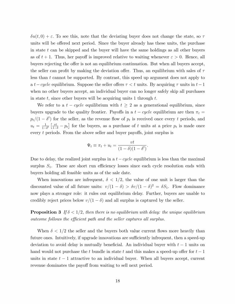
�u(t; 0) + ": To see this, note that the deviating buyer does not change the state, so �

units will be o¤ered next period. Since the buyer already has these units, the purchase

in state t can be skipped and the buyer will have the same holdings as all other buyers

as of t + 1. Thus, her payo¤ is improved relative to waiting whenever " > 0. Hence, all

buyers rejecting the o¤er is not an equilibrium continuation. But when all buyers accept,

the seller can pro�t by making the deviation o¤er. Thus, an equilibrium with sales of �

less than t cannot be supported. By contrast, this speed up argument does not apply to

a t� cycle equilibrium. Suppose the seller o¤ers � < t units. By acquiring � units in t�1when no other buyers accept, an individual buyer can no longer safely skip all purchases

in state t, since other buyers will be acquiring units 1 through t:

We refer to a t � cycle equilibrium with t � 2 as a generational equilibrium, since

buyers upgrade to the quality frontier. Payo¤s in a t � cycle equilibrium are then �t =

pt=(1 � �t) for the seller, as the revenue �ow of pt is received once every t periods, and

ut =1

1��t�vt1�� � pt

�for the buyers, as a purchase of t units at a price pt is made once

every t periods. From the above seller and buyer payo¤s, joint surplus is

t � �t + ut =vt

(1� �)(1� �t):

Due to delay, the realized joint surplus in a t� cycle equilibrium is less than the maximalsurplus S1. These are short run e¢ ciency losses since each cycle resolution ends with

buyers holding all feasible units as of the sale date.

When innovations are infrequent, � < 1=2, the value of one unit is larger than the

discounted value of all future units: v=(1 � �) > �v=(1 � �)2 = �S1. Flow dominance

now plays a stronger role: it rules out equilibrium delay. Further, buyers are unable to

credibly reject prices below v=(1� �) and all surplus is captured by the seller.

Proposition 3 If � < 1=2, then there is no equilibrium with delay: the unique equilibriumoutcome follows the e¢ cient path and the seller captures all surplus.

When � < 1=2 the seller and the buyers both value current �ows more heavily than

future ones. Intuitively, if upgrade innovations are su¢ ciently infrequent, then a speed-up

deviation to avoid delay is mutually bene�cial. An individual buyer with t � 1 units onhand would not purchase the t bundle in state t and this makes a speed-up o¤er for t� 1units in state t � 1 attractive to an individual buyer. When all buyers accept, currentrevenue dominates the payo¤ from waiting to sell next period.

18

3.2 Delay Conditions and Existence

Equilibrium delay requires that the seller can �nd no o¤er that is acceptable to buyers

and also pro�table relative to waiting to sell in state t. Thus, we will specify cut-o¤ prices

for buyer strategies such that the seller does not �nd it pro�table to make a sale before

the quality gap reaches t units.

Satisfying the buyer and seller delay incentives reduces to �nding a ut that satis�es

(1� �� )(t � ut) �v�(���t � 1)(1� �)

+ max

�v�

(1� �); ut

�� ut (5)

for � = 1; :::; t � 1. As shown in Appendix C, when ut satis�es (5), there exist cut-o¤prices that support delay. The analysis of (5) is involved because the buyer and seller

delay incentives can change signi�cantly as the quality gap rises. To begin, note that (5)

implies a lower as well as an upper bound on ut. As ut approaches 0, (5) fails at all � ,

since the incentive for an individual buyer to jump ahead is very strong and the seller can

pro�tably attract buyers as early as � = 1. If the buyers get too much of the available

surplus (ut approaches t); then (5) necessarily fails at all � : the seller can exploit �ow

dominance to sell early and pro�tably attract buyers by o¤ering � units at a price of v� .

An extreme payo¤ on either the buyer or the seller side thus allows the seller to prof-

itably induce a speed up. As a consequence, both buyer and seller payo¤s are compressed

relative to the range of payo¤s for e¢ cient equilibria.

Lemma 3 The set of payo¤s for all generational equilibria is a strict subset of the set ofpayo¤s for e¢ cient equilibria.

In order to be willing to wait until period state t; a buyer must decline seller deviation

o¤ers. This requires a strictly positive payo¤ for buyers. By contrast, there is an e¢ cient

equilibrium in which buyers receive no surplus. Similarly, the seller must be willing

to delay and this includes foregoing the option to sell units prematurely at �ow value.

Thus, the seller necessarily earns more than the �ow dominance lower bound. The upper

bounds then follow from the lower bound on the other side of the market. Thus, while

delay generates less surplus, both sides of the market necessarily receive a larger payo¤

relative to the minimum subgame perfect equilibrium payo¤.

Satisfying the delay conditions for a t � cycle equilibrium reduces to �nding a buyer

utility for the sale date, ut, that satis�es (5) for a given t and �. As the sale date gets

19

closer, buyer incentives change signi�cantly when ut lies between v1�� and

v(t�1)1�� . Initially,

for small � , a deviating buyer who acquired � units would be willing to purchase again at

the sale date t, owing to a su¢ ciently large quality increase between � and t. However,

for � closer to t, a deviating buyer would choose to fall behind the market since the

incremental surplus from t� � units is insu¢ cient.

Because of this change in buyer deviation incentives, the delay conditions may bind at

an interior � . While a complete characterization of (5) is quite involved, it turns out that

many of the complications only arise at relatively low discount factors.10 In Appendix C,

we develop a su¢ cient condition on �t such that if �t is above a threshold, d�, then the

delay conditions (5) are satis�ed for an interval,�uA; uA

�; of utility levels. We then have

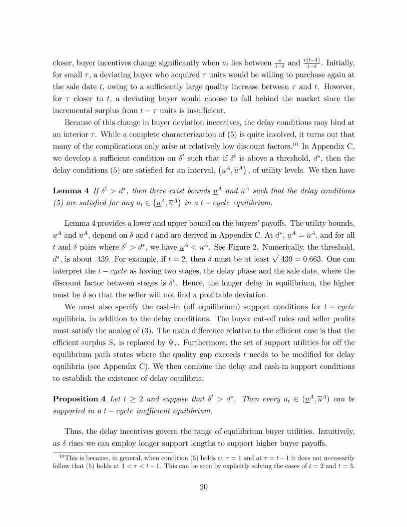
Lemma 4 If �t > d�, then there exist bounds uA and uA such that the delay conditions

(5) are satis�ed for any ut 2�uA; uA

�in a t� cycle equilibrium.

Lemma 4 provides a lower and upper bound on the buyers�payo¤s. The utility bounds,

uA and uA, depend on � and t and are derived in Appendix C. At d�, uA = uA, and for all

t and � pairs where �t > d�; we have uA < uA. See Figure 2. Numerically, the threshold,

d�, is about :439. For example, if t = 2; then � must be at leastp:439 = 0:663. One can

interpret the t� cycle as having two stages, the delay phase and the sale date, where thediscount factor between stages is �t. Hence, the longer delay in equilibrium, the higher

must be � so that the seller will not �nd a pro�table deviation.

We must also specify the cash-in (o¤ equilibrium) support conditions for t � cycle

equilibria, in addition to the delay conditions. The buyer cut-o¤ rules and seller pro�ts

must satisfy the analog of (3). The main di¤erence relative to the e¢ cient case is that the

e¢ cient surplus S� is replaced by � . Furthermore, the set of support utilities for o¤ the

equilibrium path states where the quality gap exceeds t needs to be modi�ed for delay

equilibria (see Appendix C). We then combine the delay and cash-in support conditions

to establish the existence of delay equilibria.

Proposition 4 Let t � 2 and suppose that �t > d�. Then every ut 2 (uA; uA) can besupported in a t� cycle ine¢ cient equilibrium.

Thus, the delay incentives govern the range of equilibrium buyer utilities. Intuitively,

as � rises we can employ longer support lengths to support higher buyer payo¤s.

10This is because, in general, when condition (5) holds at � = 1 and at � = t�1 it does not necessarilyfollow that (5) holds at 1 < � < t� 1. This can be seen by explicitly solving the cases of t = 2 and t = 3.

20

•

1

uA

uA

δd*

ut

BuyerPayoff

0.5

1.44

.663 =

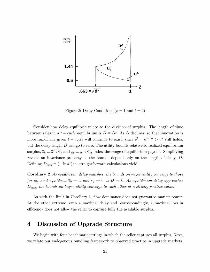
Figure 2: Delay Conditions (v = 1 and t = 2)

Consider how delay equilibria relate to the division of surplus. The length of time

between sales in a t � cycle equilibrium is D � �t. As � declines, so that innovation is

more rapid, any given t � cycle will continue to exist, since �t = e�r�t > d� still holds,

but the delay length D will go to zero. The utility bounds relative to realized equilibrium

surplus, sb � uA=t and sb � uA=t, index the range of equilibrium payo¤s. Simplifying

reveals an invariance property as the bounds depend only on the length of delay, D.

De�ning Dmax � (� ln d�)=r, straightforward calculations yield:

Corollary 2 As equilibrium delay vanishes, the bounds on buyer utility converge to thosefor e¢ cient equilibria, sb ! 1 and sb ! 0 as D ! 0: As equilibrium delay approaches

Dmax, the bounds on buyer utility converge to each other at a strictly positive value.

As with the limit in Corollary 1, �ow dominance does not guarantee market power.

At the other extreme, even a maximal delay and, correspondingly, a maximal loss in

e¢ ciency does not allow the seller to capture fully the available surplus.

4 Discussion of Upgrade Structure

We begin with four benchmark settings in which the seller captures all surplus, Next,

we relate our endogenous bundling framework to observed practice in upgrade markets.

21

We then discuss our results relative to assumptions in the upgrade literature.

4.1 Benchmarks

First, consider a �nite horizon. Once the �nal period arrives, buyers have no prospect

of acquiring upgrades in the future. Subgame perfection then implies that each buyer

will necessarily accept any o¤er that provides a positive payo¤. The unique equilibrium

outcome in the �nal period, given any current units held by the buyers, is that the seller

o¤ers an upgrade to the state of art at a price equal to the full value of the upgrade to the

buyers. By backward induction, this holds for all prior periods since buyers never expect

a positive payo¤ in the future. Hence, the equilibrium follows the e¢ cient path and the

seller captures the full social surplus.11

Second, suppose that there is no surplus growth: the seller has one unit to o¤er and

trade may take place at any time over an in�nite horizon. With no heterogeneity among

buyers, we have a special case of the standard durable goods model (gap case). The

result of Fudenberg, Levine, and Tirole (1985) implies that there is never delay and the

full surplus is always extracted from buyers in any subgame perfect equilibrium.

Suppose that there is only one buyer in an in�nite horizon model with growth. A

variation on the speed-up argument of Fudenberg, Levine, and Tirole implies that the

seller can always pro�tably tempt the buyer to purchase all available units immediately.

The choice of a single buyer necessarily changes the state, in contrast to the case with a

continuum. When responding to a current o¤er, a refusal is optimal only if the discounted

continuation payo¤ exceeds the payo¤ from accepting the o¤er. Then a positive buyer

payo¤, u1 > 0, requires a supporting utility path that rises inde�nitely at an exponential

rate. Because this exceeds the available surplus in �nite time, a credible threat for refusing

a price increase, relative to u1, unravels. The only equilibrium has u1 = 0.

Finally, with a complete absence of complementarity across quality levels, units 1; 2; :::

are independent goods. Then, as one might expect, the seller regains the ability to

extract buyers due to the lack a credible threat. The essential di¤erence is that a buyer

can accept a current o¤er when others do not, skip the subsequent cash-in o¤er from

the seller, and then resume purchasing. Because the goods are independent, there is no

payo¤ consequence due to complementarity from any missing units. Thus, we necessarily

have u1 = 0. Intuitively, complementarity is essential for a credible threat to refuse price

increases as a deviating individual buyer faces the extra cost of having to acquire the

11Further details on this and the other benchmarks are provided in the working paper version.

22

missing unit. This is why, in our upgrade structure, it matters to an individual buyer

whether or not others are expected to purchase the seller�s o¤er.

Thus, as all four benchmarks lead to strong monopoly power, each element is essential

to a credible threat for buyers in an upgrade market.

4.2 Bundling in Practice

In practice, the upgrade process varies greatly with respect to how buyers move to

higher quality levels. Contract contingencies, especially with respect to a buyer�s current

holdings, are frequently observed. MacKichan, for example, o¤ers the technical word

processor Scienti�c Word 5.5 in a number of versions di¤erentiated by features and each

version has an upgrade price for prior users (serial number required) as well as a (higher)

price for new users. Airliners typically o¤er seat upgrades, club memberships, and other

amenities at prices that vary with frequent �ier status, a result of past purchases.

A new version with a price contingent on a buyer�s current version is very close and

often will be equivalent to an upgrade o¤er. Consider a buyer who holds units f1; :::; �gand two o¤ers. One is an upgrade bundle f� + 1; :::; � + kg for price p: The other is anew version f1; :::; �; :::; � + kg at price p that is only available to buyers who hold unitsf1; :::; �g. The direct value to the buyer is the same with either bundle. Now, considerthe same o¤ers, but suppose that the buyer does not hold any units. By downward

complementarity, the upgrade bundle has no direct value (non-contiguous units) while the

buyer does not qualify for the other o¤er. Further, observe that if the pricing contingency

is stated as a minimum requirement then buyers who hold at least the minimum will

place a common value on the two bundles. Such a minimum requirement is common in

practice. Microsoft allows any 2000-2007 O¢ ce program or suite to qualify a buyer for

O¢ ce Professional at the upgrade (discount) price.

Thus, our equilibria will be robust to allowing price contingencies if we can demonstrate

that it is still optimal for the seller to make the same o¤ers (either in the upgrade form or

the appropriate version form with a holding contingency). Consider the possibility that,

by conditioning o¤ers on current holdings, a seller may be able to curtail the credible

threat of buyers to reject o¤ers with high prices and thus eliminate equilibria with low

seller payo¤s. In this regard, our equilibria are robust. First, recall that buyers all have the

same holdings on any equilibrium path and a contractual contingency in this regard has no

force. With respect to the support for the equilibrium path, the same observation applies

to the cash-in support. Finally, when buyers have asymmetric holdings, we constructed

23

continuation equilibria in which the seller captured the available surplus and, as a result,

this support is robust to the addition.

At a more intuitive level, recall that the credible threat to reject seller o¤ers with

high prices is based on the expectation of a su¢ ciently high future surplus (when all

buyers reject the o¤er). Consider, for example, the support condition (3) for an e¢ cient

equilibrium and the impact of allowing contract contingencies on buyer holdings. An

individual buyer who fails to purchase when others do will fall behind the equilibrium

path, but such a buyer is already extracted in our analysis. On the other hand, a buyer

who purchases when others do not will jump ahead of the market and, in our analysis, such

a buyer does have a strict preference for purchasing the subsequent equilibrium support

cash-in o¤er from the seller. The seller could then employ a contractual contingency to

isolate such a buyer and eliminate the (valuable) option to accept an o¤er designed for

buyers with fewer units and �rejoin�the equilibrium path. But if the contingency is used

to make an o¤er that extracts the deviating buyer then this will only serve to reduce

further the deviation payo¤ to purchasing when others do not (refer to the max condition

for g(� ; �) in (3)). Thus, the support condition (3) continues to be satis�ed by our T -stage

utility path and buyers retain a credible threat.

Thus, whether we regard the o¤ers as upgrade bundles or versions with price contin-

gencies, as in Fudenberg and Tirole (1998) or Ellison and Fudenberg (2000), does not

a¤ect the equilibrium structure.12 In terms of information structures, our original o¤er

set corresponds to the semi-anonymous regime of Fudenberg and Tirole (1998), where

harsher terms cannot be imposed on buyers who hold more units than others. This estab-

lishes that our results do not depend on the precise form of the seller�s o¤ers.13 Bundles

can be presented as upgrades or as versions with a contingency on past purchases. Our

formulation of the o¤er space is simpler as it avoids the complications of contingencies.

4.3 Unbreakable version o¤ers

Suppose that, as an exogenous condition, all bundles must be versions and no contin-

gencies on purchase are allowed. That is, any o¤er for the current quality increment, unit

12In both Fudenberg and Tirole and Ellison and Fudenberg the second period o¤ers can distinguishbetween buyers who purchased in period 1 and those who did not. These models also feature buyerheterogeneity.13In our working paper we also address network e¤ects, compatibility issues, and adoption costs. We

argue that our equilibrium results are robust to these forces as they all reinforce the incentive for a buyerto keep up with the market while reducing the payo¤ of a buyer who jumps ahead of the market. See therelated policy discussion in Anton and Biglaiser (2010a).

24

� , is necessarily also an o¤er for units f1; :::; �g and similarly for any lower quality level.This might re�ect a necessary property of the production technology, where a quality

increment cannot be �broken out�for separate sale. This o¤er structure is examined in

Waldman (1996) for a two-period model and in Fishman and Rob (2000) for an in�nite

horizon model, both of whom focus on innovation incentives.

In our setting, where buyers have identical preferences, this �unbreakable� upgrade

structure necessarily limits the market power of the seller. The reason is that a buyer

always has the option of passing on a current o¤er and waiting to purchase a later o¤er.

As long as the seller eventually o¤ers a higher quality, the cost of waiting (relative to

purchasing when other buyers do) is the lost �ow value. Any subsequent higher-quality

o¤er that attracts prior buyers will necessarily provide the buyer who delays with a strictly

larger surplus than that received by prior buyers. As a result, there is no equilibrium in

which a monopoly seller captures the full surplus when upgrades are unbreakable.

In a two-period version of our model and unbreakable goods, it is straightforward to

derive the equilibrium. For large discount factors, the seller delays until period 2 and

then o¤ers units f1; 2g at the extraction price for the remaining surplus. For low discountfactors, however, unit 1 is sold in period 1 for v and then period 2 has extraction pricing

for units f1; 2g. The seller is never able to capture the full surplus, in contrast to the �nitehorizon equilibrium with upgrade o¤ers or generation o¤ers with price contingencies.

In the case of an in�nite horizon with non-contingent pricing, ongoing quality growth

necessarily imposes a more severe limit on the seller. Fishman and Rob (2000) point out

that the option to wait implies that the seller can charge no more than the �ow value.14

In their rational expectations equilibrium, the low price leads to a rate of innovation that

is ine¢ ciently low. In our analysis, where bundling is endogenous, the option to wait (fall

behind the market) is inconsequential. The basis of a credible threat for buyers resides

with the extent to which the seller can tempt a buyer to jump ahead of others.

14Full extraction of total surplus by the seller requires implementing the e¢ cient path and, in theunbreakable version of our model, the seller would be limited to prices that re�ect only the �ow value andnot the present discounted value to buyers from quality increments. Formally, consider the e¢ cient pathand let p(� ; ��1) be an equilibrium price for version � when all buyers hold f1; :::; � � 1g. By rejecting ano¤er and resuming purchases next period, an individual buyer obtains v (� � 1)+�u(�+1; �). Purchasingtoday yields v� � p(� ; � � 1) + �u(� + 1; �). Combining, we must have p(� ; � � 1) � v.

25

5 Directions for Future Work

Buyers are homogeneous in our model. This was assumed to focus on the structure

of credible threats for buyers in a dynamic upgrade model in what one would expect to

be the ideal situation for a seller to capture the full (e¢ cient) joint surplus. Allowing

for buyer heterogeneity is an important direction for subsequent work. In practice, it is

common for sellers in upgrade markets to o¤er simultaneously di¤erent versions or quality

levels of their products. This is typically taken to be a form of price discrimination. As

noted before, several papers examine a �nite horizon model, but there has been very little

theoretical work on in�nite horizon models in which buyers are always in the market and

quality improvements are ongoing. One could introduce buyer heterogeneity in our model

where buyers are privately informed of their valuation. This allows for an endogenous

determination of pricing and whether the buyer segments remain distinct over time or

whether the seller chooses to price over a cycle that periodically brings high and low

types together at a common quality level (a generational cycle). An interesting feature of

equilibrium price discrimination in this dynamic context is that incentive constraints can

bind in both directions (with low-value buyer types choosing to mimic high-value buyer

purchases as well the standard downward incentive constraint).

We also assumed an exogenous rate for the increase in quality. Of course, a model that

addresses the question of how rewards for a given quality innovation are determined is a

necessary step toward an endogenous determination of quality change. We are currently

studying innovation and pricing incentives in a model where innovations can be generated

not only by an incumbent but also by potential entrants. In this setting, property rights

for innovation in relation to imitation incentives are crucial for buyer decisions regarding

adopting the products of an incumbent or an entrant and, in turn, for assessing public

policy choices and welfare in upgrade markets.

References

[1] Anton, James J., and Gary Biglaiser. 2010a. �Compatibility, Interoperability, and

Market Power in Upgrade Markets.�Economics of Innovation and New Technology,

19(4): 373-85.

[2] Anton, James J., and Gary Biglaiser. 2010b. �Quality, Upgrades and Equilibrium in

a Dynamic Monopoly Market.�Working paper.

26

[3] Ausubel, Lawrence M., and Raymond J. Deneckere. 1989. �Reputation in Bargaining

and Durable Goods Monopoly.�Econometrica, 57(3): 511-31.

[4] Bond, EricW., and Larry Samuelson. 1984. �Durable GoodMonopolies with Rational

Expectations and Replacement Sales.�RAND Journal of Economics, 15(3): 336-45.

[5] Bulow, Jeremy I. 1982. �Durable-Goods Monopolists.�Journal of Political Economy,

90(2): 314-32.

[6] Coase, Ronald H. 1972. �Durability and Monopoly.�Journal of Law and Economics,

15(1): 143-49.

[7] Ellison, Glenn, and Drew Fudenberg. 2000. �The Neo-Luddite�s Lament: Excessive

Upgrades in the Software Industry.�RAND Journal of Economics, 31(2): 253-72.

[8] Fehr, Nils-Henrik, and Kai-Uwe Kuhn. 1995. �Coase versus Pacman: Who Eats

Whom in the Durable-Goods Monopoly?�Journal of Political Economy, 103(4): 785-

812.

[9] Fishman, Arthur, and Rafael Rob. 2000. �Product Innovation by a Durable Goods

Monopoly.�RAND Journal of Economics, 31(2): 237-52.

[10] Fudenberg, Drew, and Jean Tirole. 1991. Game Theory. Cambridge, MA: MIT Press.

[11] Fudenberg, Drew, and Jean Tirole. 1998. �Upgrades, Tradeins and Buybacks.�RAND

Journal of Economics, 29(2): 235-58.

[12] Fudenberg, Drew, David Levine, and Jean Tirole. (1985), �In�nite Horizon Models

of Bargaining with One-Sided Incomplete Information.�In Game Theoretic Models

of Bargaining, ed. Alvin E. Roth, 73-98. Cambridge: Cambridge University Press.

[13] Gul, Faruk, Hugo Sonnenschein, and Robert Wilson. 1986. �Foundations of Dynamic

Monopoly and the Coase Conjecture.�Journal of Economic Theory, 39(1): 155-90.

[14] Hoppe, Heidrun and In Ho Lee. 2003. �Entry Deterrence and Innovation in Durable-

Goods Monopoly.�European Economic Review, 47(6): 1001-1036.

[15] Maskin, Eric, and Jean Tirole. 2001. �Markov Perfect Equilibrium I: Observable

Actions.�Journal of Economic Theory, 100(2): 191-219.

27

[16] Nahm, Jae. 2004. �Durable-Goods Monopoly with Endogenous Innovation.�Journal

of Economics and Management Strategy, 13(2): 303-19.

[17] Sobel, Joel. 1991. �Durable Goods Monopoly with Entry of New Consumers.�Econo-

metrica, 57(5), 1455-85.

[18] Stokey, Nancy L. 1981. �Rational Expectations and Durable Goods Pricing.�Bell

Journal of Economics, 12(1): 112-28.

[19] Waldman, Michael. 1996. �Planned Obsolescence and the R&D Decision.�RAND

Journal of Economics, 27(3): 583-95.

[20] Waldman, Michael. 2003. �Durable Goods Theory for Real World Markets.�Journal

of Economic Perspectives, 17(1): 131-54.

6 Appendix

6.1 Appendix A - Formal Structure

We present the formal structure of the model. First, we de�ne bundles and o¤ers.

Next, we de�ne strategies and histories, present payo¤s and formally de�ne equilibrium.

(i) The Bundle O¤er Structure.

Consider the feasible o¤er set for the seller in period � . Let P� � P(f1; 2; :::; �g)denote the power set for the �rst � integers. Any set z 2 P� is called a bundle. Ano¤er is a collection of bundles and associated (non-negative) prices, (z; pz)z2Z for some

Z 2 P(P� ). De�ne the o¤er set � by

� � f! 2 P(P� �R+) j (i) (?; 0) 2 !; (ii) if (z; p) 2 ! and (z; p0) 2 !, then p = p0g :

By (i), we are including the null bundle in every o¤er by the seller. This is for two

reasons: �rst, the seller can make no o¤er by choosing only the null bundle and, second,

it streamlines the buyer choice formalism, as a buyer chooses to make no purchase by

selecting the null bundle. By (ii), every o¤ered bundle has a unique price. Clearly, if two

prices were o¤ered for the same bundle, no buyer would choose the higher price (buyers

act as price takers due to the zero measure property for strategies across histories). An

acceptance by a buyer is an element of the set P(P� ).

28

Consider the maximal contiguous quality. For any z 2 P� , de�neM : P� ! f0; 1; :::; �gby �nding the unique m 2 f0; :::; �g such that m0 2 z 8m0 � m and m + 1 =2 z, and set

M(z) = m: Clearly, M(z) is the maximal contiguous quality held by a buyer and M(z)

exists for any bundle z. For an arbitrary sequence of holdings z� , de�ne q� =M(z� ).

(ii) Strategies and Histories.

A (pure) strategy for the seller is a sequence of o¤ers, O = (O� ). Each o¤er is a mapfrom the history of play up through period � � 1 into the o¤er set � . A history is thesequence of previous o¤ers by the seller and acceptances by the buyers. LettingH� denote

the space of all histories up through period � � 1, we have

O� : H� ! � :

Given an observed history, h� 2 H� , the seller�s strategy speci�es an o¤er !� = O� (h� ) :A buyer (pure) strategy pro�le is a sequence of acceptance decisions, A = (A� ). Given

a history h� and a seller o¤er !� , each buyer x 2 [0; 1] needs to choose which bundles in!� to accept. Thus, we have acceptance strategies for each buyer

Ax� : H� � � ! P(P� ):

Hence, for observed history h� 2 H� and in response to a seller o¤er of !� 2 � , buyerx chooses to accept the set of bundles Ax� (h� ; !� ) � P(P� ). Of course, any acceptedbundle, z 2 Ax� (h� ; !� ), must have been o¤ered by the seller, (z; p) 2 O� (h� ) for somep. This is a feasibility restriction. Note that a buyer is free to accept one or more of the

bundles (i.e., any subset) included in an o¤er !� . For example, by �accepting�only the

null bundle, a buyer makes no purchase in period � . Finally, we use A� for the strategypro�le across buyers.

We need to specify the history space H� . First, de�ne � � 1 � 2 � ::: � � ;this product space contains each feasible sequence of previous o¤ers. Second, we need to

calculate acceptance sets from buyer bundle purchases and this entails a measurability

assumption on buyer strategies.

Let F� denote the set of Borel measurable functions for [0; 1]! P(P� ). By de�nition,f� : [0; 1] ! P(P� ) is Borel measurable (that is, f� 2 F� ) if for any z 2 P� we haveX� (z) 2 B (the Borel sets of [0; 1]), where X� (z) = fx 2 [0; 1] j z 2 f� (x)g. Thus, the setof buyers who chose bundle z is a Borel set and we can calculate market share and revenues

by using standard Lebesgue measure. De�ne the product space F �� F1 �F2 � :::�F� .

29

Then the history space is speci�ed by H 1 = ? and for � > 1,

H� = ��1 �F ��1:

Note that the bundles and prices o¤ered by the seller are recorded in ��1 while the

bundles accepted by each buyer are recorded in F ��1. Thus, we know the price a buyer

paid for a bundle from the history. We assume that for each h� 2 H� , and !� 2 � , wehave A� 2 F� , i.e. Ax� (h� ; !� ) is a Borel measurable function on x 2 [0; 1]. An equivalent,but less convenient, formulation would be to assign an index to each element in the �nite

set P(P� ) and de�ne measurability in the standard way for a real valued function.(iii) Payo¤s and Equilibrium.

Turning to the calculation of player payo¤s, we begin with the buyers. First, for each

h�+1, calculate the units acquired by buyer x in each period k = 1; :::; � . These units are

given by Zk(x) = fi 2 f1; :::; kg j i 2 z for some z 2 Axk(hk; !k)g, the bundles accepted bybuyer x. Thus, the set of units that buyer x has accumulated through the end of period

� is given by

Z� (x) ��[k=1

Zk(x) � P� :

Recalling thatM(z) is the maximal contiguous quality for any subset z of f1; :::; �g, we seethat the maximal contiguous quality unit held by buyer x is given by m� (x) �M(Z� (x)).

Next, the total expenditure of buyer x in period � is given by p� (x) �P

z2Ax� (h� ;!� )pz,

which is the sum of the payments for each bundle that the buyer accepted. Thus, the

payo¤ to buyer x from strategy Ax when other buyers follow A�x and the seller followsO is the present discounted value of surplus from the maximal unit held less expendituresin each period:

U(O;Ax;A�x) =1X�=1

���1 [vm� (x)� p� (x)] :

The in�nite sum is always well de�ned, since (i) the sequence of maximal holdings m� is

non-decreasing in � , (ii) m� � � , and (iii)1X�=1

���1� = 1= (1� �)2.

We now compute the seller payo¤. Given a history and an o¤er by the seller, X� (z)as de�ned above is the set of buyers for whom z 2 Ax� (h� ; !� ). The Lebesgue measure of

30

such buyers is �� (z) �R

X� (z)dx. Thus, the revenue of the seller in period � is

r� =Pz2P�

�� (z)pz:

�� (z) = 0 must hold if the seller did not o¤er bundle z or if no buyer purchased z.

The seller payo¤ under strategies (O;A) is then

�(O;A) =1P�=1

���1r� :

The de�nitions for Nash and subgame perfect equilibrium are standard. The strategies

(O;A) form a Nash equilibrium if

�(O;A) � �( bO;A) for all bO;U(O;Ax;A�x) � U(O; bAx;A�x) for all bAx:

A subgame perfect equilibrium requires that (O;A) form a Nash equilibrium at any

given h� ; where the seller makes an o¤er, and at any given h� and !� , where the buyers

respond to the o¤er.

When buyers are distributed across maximal holdings, the state is given by (� ,(Qm� )m=0;:::;��1),

where Qm� is the set of buyers with maximal contiguous quality m: More generally,

when buyers are distributed as (Qm� )m=0;1:::;� , then the translated state is given by (� +

1�m� ,(Qm� )m=m� ;:::;�) where m� is the smallest index of Q

m� with a non-zero measure.

6.2 Appendix B - E¢ cient Equilibria

We �rst prove Lemmas 1 and 2 and then state several lemmas dealing with properties

of the T � stage support. This is followed by the proof of Proposition 1.

(i) Flow Dominance and Su¢ cient Conditions for Equilibrium

Proof of Lemma 1. Depending on the history, buyers may also hold a subset, possibly

null, of units fQ+ 2; :::; � � 1g. Without unit Q + 1, a buyer who rejects the upgradeo¤er will receive a �ow payo¤ of vQ and have the same quality holdings in period � + 1:

A buyer who accepts will receive a �ow payo¤ of v� in period � and hold f1; :::; �g nextperiod. We will show that accepting yields a strictly higher payo¤ than rejecting, for any

strategy choices of other buyers and the seller following the upgrade o¤er.

Obviously, accepting yields a higher �ow payo¤in period � since v��p > vQ. Consider

31

the continuation payo¤. An accepting buyer (i) begins with more units than a non-

accepting buyer and (ii) has the option of mimicking the strategy of any non-accepting

buyer (any seller o¤er may purchased by any buyer). By the upgrade payo¤ structure,

the continuation payo¤ of an accepting buyer is therefore at least as large as that of a

non-accepting buyer. This is because the mimicking option implies the same payments,

but the accepting buyer will never hold fewer units.

It is now clear that every buyer will choose to accept the upgrade o¤er. Given any

strategy choices of other buyers and the seller following the upgrade o¤er, a buyer who

accepts always has a weakly larger payo¤ from �+1 onward, with respect to the continua-

tion sequence of o¤ers implied by the strategies, and a strictly larger �ow payo¤ in period

� . By the zero measure property, the continuation sequence of o¤ers does not depend on

the choice of a speci�c individual buyer to accept or reject the upgrade o¤er. �Proof of Lemma 2. To establish existence of an equilibrium we need to show that

(i) our candidate upgrade o¤er is optimal for the seller with respect to the o¤er set

� , and (ii) construct a continuation equilibrium for states where buyers are distributed

asymmetrically providing, for any such state, both an optimal o¤er for the seller and

optimal buyer responses for any given seller o¤er.

Now, de�ne an upgrade o¤er B as any o¤er in � , with the property that if (z; pz) 2 B,then M(z) = supfi j i 2 z g. By construction, every bundle in B is an upgrade bundle,since the maximal contiguous quality in z coincides with the largest quality unit in z.

Thus, we can denote any (z; pz) 2 B by (b; pb) ; where b � supfi j i 2 zg is the upgradelevel for z and pb � pz is the price. An upgrade o¤er need not include all of the feasible

upgrade bundle levels 1; :::; � . A buyer will optimally choose at most one bundle in B.The restriction to upgrade o¤ers can be shown to be without loss of generality. This

is because we construct continuation equilibria in which only upgrade o¤ers are made

by the seller. Thus, even if a period � o¤er includes non-upgrade bundles, all players

expect that every possible period � +1 continuation state will involve only upgrade o¤ers.

Furthermore, in every possible period � + 1 continuation state, every buyer will move to

a quality holding of at least � in the continuation equilibrium outcome. Consequently, a

buyer will value bundles in an o¤er only to the extent that the bundle allows the buyer

to move to a higher quality level in period � . If a buyer�s purchases in � result in the

acquisition of non-contiguous quality levels, these non-contiguous units have no current

or future payo¤ e¤ect due to the structure of the continuation equilibria.

More generally, if buyers are asymmetrically distributed across maximal quality levels

32

and if buyers hold non-contiguous quality units (above a buyer�s maximal level), we can

still work with upgrade o¤ers without loss of generality. This is because any o¤er in

conjunction with a buyer�s current maximal quality and non-contiguous holdings can

always be reduced to an implied set of payments for achievable (higher) maximal quality

levels. With the continuation equilibria noted above, any resulting non-contiguous quality

units will have no payo¤ impact.

To demonstrate (i), it is su¢ cient to show that the seller cannot pro�tably deviate in

state (� ; 0) to some other upgrade o¤er (with multiple upgrade bundles). First, de�ne a

buyer preference relation, �B, for any two upgrade bundles by

(b; pb) �B (i; pi) () vb� pb + �u(� + 1; b) � vi� pi + �u(� + 1; b j i);

where u(� + 1; b j i) is equal to vi1�� if i < b and equal to max

�vi1�� ; u(� + 1; b)

if i � b.

Note that the �B relation re�ects implicit coordination in that an individual buyer hasno incentive to choose (i; pi) if all other buyers choose (b; pb). Now, de�ne an upgrade

(b; pb) 2 B to be a buyer continuation equilibrium (BCE) in state � for o¤er B if (b; pb) �B(i; pi) 8 (i; pi) 2 B. We must show that for any o¤er B there exists a BCE such that theseller cannot gain in state � by deviating to o¤er B instead of making the cash-in o¤erof p� . The proof is lengthy so we only provide a sketch. First, one shows that any two

upgrade o¤ers are comparable under �B. Next, one can show that

arg max(b;pb)2B

�vb

1� �� pb + �u�+1�b

�is a BCE (existence is trivial as B has a �nite number of bundles; if it is not unique thenselect the argmax with largest upgrade level). Essentially, this follows because the argmax

is the highest possible coordinated payo¤ for buyers and because utility di¤erences across

a T -stage support satisfy the bound u� � u�0 � v(���0)1�� .

We then have two cases for the o¤er B. If every (b; pb) 2 B satis�es pb � Gb �g(b; u�+1), then it is easy to show that (0; 0), where all buyers refuse to purchase, is a

BCE for B. This is equivalent to a delay outcome and we know from (3) that the seller

prefers to make the cash-in o¤er p� . If pb < Gb for some (b; pb) 2 B then we �rst �nd theargmax speci�ed above for the subset of all such bundles in B, call it (b�; pb�). We thenshow that (b�; pb�) �B (i; pi) 8 (i; pi) where pi � Gi. Then, (b�; pb�) is a BCE for B andthe seller payo¤ of pb� + �u�+1�b� is, by (3), not pro�table relative to p� .

Consider (ii) and any state in which buyers are asymmetrically distributed across

33

quality levels. Since all buyers with the same maximal contiguous quality level are treated

identically in the continuation it is su¢ cient to keep track only of market shares. Thus, let

us denote such a state by (� ; �) where � = (�0; :::; ���1) speci�es for each � = 0; :::; � � 1the fraction �� 2 [0; 1] of buyers entering period � with maximal quality level of �. Byhypothesis, 1 > �0 > 0 and

P��1�=0 �� = 1. We specify a continuation equilibrium for

(� ; �) as follows. The seller makes an upgrade o¤er f(b�; p�)g�=0;:::;��1 where each (b�; p�)is an upgrade from � to � , that is the bundle f� + 1; :::; �g, for price

p� =v(� � �)

1� �+ �u1:

For buyer strategies, we specify that a buyer with � units chooses to accept (b�; p�). It is

straightforward to verify that, when all other buyers follow this strategy, it is optimal for

an individual buyer with � to do so as well. Since these upgrade o¤ers leave each buyer

with a payo¤ of v�= (1� �), the payo¤ to the seller is equal to the continuation surplus

of S� less these individual-rationality payo¤s aggregated across buyers according to the

distribution �. By feasibility, this bounds the seller�s payo¤ in any continuation.

Finally, to complete the argument that the above upgrade o¤er is an optimal choice for

the seller, we need to specify a BCE if the seller makes some other upgrade o¤er. Allow-

ing for partial upgrades, denote such an o¤er by B = f(b; �; pb;�) j � � b � � ; 0 � pb;�g in(� ; �), where each (b; �; pb;�) denotes an upgrade bundle for units f� + 1; :::; bg at price pb.Since the o¤er B has upgrades that begin at di¤erent levels and a buyer is free to purchasemultiple bundles, we construct from B for each possible buyer quality level � = 0; :::; ��1,the set B� of all upgrade bundles that move � to a higher quality level; note B� mightcontain only the refusal option for some �: We then have each buyer with quality level �

choose to accept the (largest index)

argmaxB�

�vb

1� �� pb;�0

�:

Then, these choices can be shown to form a BCE for B. The proof is trivial if the buyerchoices result in a nondegenerate distribution across quality levels since the buyers are

then held to their individual-rationality payo¤s in the continuation state. If not, then

all buyers move to some common quality level, say b, and we must use the continuation

payo¤ u�+1�b from the T -stage support. �(ii) Properties of the T � stage Support

34

Lemma A1 Consider a T -stage support, where u� = uT � u for � � T . If the support

condition (3) holds at � = T for � = 0; :::; T , then (3) holds at � > T for � = 0; :::; � .

Lemma A2 Consider a T � stage support. Then for any � � T , we have

u� =1

���1

�u1 �

v

1� �

�1� ���1

1� �� (� � 1)���1

��:

Lemma A3 The T � stage support sequence (u1; :::; uT ) de�ned by u1 = (1� �T�1)S1satis�es (i) u� =

�1� �T��

�S1 +

v(��1)1�� , (ii) u� �

v�1�� if and only if � � �T�� and (iii)

uT�1 � v(T�1)1�� and uT�2 � v(T�1)

1�� � v.

Lemma A4 Consider a T � stage support with (i) u� � v�1�� for � = 1; :::; T � 1 and

(ii) v(T�1)1�� < uT <

vT1�� . If the support condition (3) holds at (� ; �) for � = 1; :::; T , then

the T � stage support satis�es (3) for all (�; �), where 0 � � � � and � � 1.(iii) Existence of Equilibrium

Proof of Proposition 1. First, note that conditions (i) and (ii) of Lemma A4 are valid

when�1� �T�1

�S1 � u1 �

�1� �T

�S1. This follows by applying Lemma A3 to the

reference sequences, u� , for T and for T +1. Then, by Lemma A4, it is su¢ cient to verify

condition (3) at (� ; �) for � = 1; :::; T .

It is immediate that (3) at � = 1 requires �S1 � u1. Hence, we are done if T = 1.

Now, consider T � 2 and note that the same observation implies that (3) holds at (1; 1).Now, consider (3) at (� ; �) for � � T �1. Then u�+1 > v�

(1��) and we have g(� ; u�+1) =

v� . Thus, the equilibrium support condition (3) becomes

�v�

1� �+ �u1 � u� .

We claim that condition (� ; �) implies condition (�+1; �+1) for � � T�2. In other words,we claim that �v�

1�� +�u1 � u� implies�v(�+1)1�� +�u1 � u�+1. Recall that u�+1 = 1

�(u� � v�).

So, condition (� + 1; � + 1) can be written as

�2v(� + 1)

1� �+ �2u1 + v� � u� .

Thus, it is su¢ cient to show that �2v(�+1)1�� + �2u1 + v� >

�v�1�� + �u1. But, this holds if and

only if �S1 + v��> u1, which is always the case for � � 1. Thus, (3) holds at (1; 1) and

this implies (3) holds at (� ; �) for � = 2; :::; T � 1.

35

We are then left with the (T; T ) condition, which reduces to

�u1 � (1� �)uT ,

since g(T; uT+1) = vT1�� � �uT by Lemma A3. We know that the condition holds at

(T � 1; T � 1) and we have

�v(T � 1)1� �

+ �u1 � uT�1 = v(T � 1) + �uT ,

1

�

��v(T � 1)1� �

� (T � 1)v + �u1

�� uT :

Thus, it is su¢ cient for (T; T ) to show that

�

1� �u1 �

1

�

��v(T � 1)1� �

� (T � 1)v + �u1

�: (6)

Simplifying and noting that � � 1=2, condition (6) holds if and only if �u1 � v(T � 1):From u1 � (1 � �T�1)S1, it is su¢ cient to show that �(1 � �T�1)S1 � v (T � 1). At

T = 2 this reduces to � � 1=2. Now, we carry out an induction: assume it holds for T

if � + �T�1 > 1 and show that it holds for T + 1 if � + �T > 1. So, we must show that

�(1� �T )S1 � vT or, equivalently, that

�(1 + :::+ �T�1) > T (1� �):

The condition at T is �(1� �T�1)S1 � v (T � 1), which holds if and only if

(1� �) + �(1 + :::+ �T�2) > T (1� �):

�(1 + :::+ �T�1) > (1� �) + �(1 + :::+ �T�2), � + �T > 1

then establishes the induction. Thus, the (T; T ) condition holds, and we have therefore

shown that the T�stage support satis�es (3) for all (�; �), where 0 � � � � and � � 1.To see that every buyer payo¤, u1 2 [0; �S1] can be supported in this way, simply

note that each � 2 [1=2; 1] lies in exactly one of the �� cuto¤ sequence intervals. Notethat the cut-o¤ sequence �� is strictly increasing in � , from �1 = 1=2 to lim�!1 �� = 1,

and satis�es ���1 < 1 � � < �� for � 2 (���1; �� ): With � 2 [�� ; ��+1), we then see thatevery u1 2 [0; �S1] lies in exactly one of the

��1� �T�1

�S1;�1� �T

�S1�intervals, where

36

T ranges from 1 up to the index on the �� root. �

6.3 Appendix C - Delay and Generational Equilibria

First we prove Propositions 2 and 3. Next, we examine the delay conditions and then

provide the analysis of the o¤ equilibrium support. Finally, we prove Proposition 4.

(i) Proofs of Propositions 2 and 3.

Proof of Proposition 2. By Lemma 1 we have �1 > 0 in any equilibrium and therefore

there is a �rst date, say t, at which a sale involving unit 1 takes place. If t = 1, we

are done as equilibrium implies we have a 1-cycle equilibrium. So, consider t > 1. By

construction, the maximal quality held by buyers before period t is zero, so the state

is t and qt > 0 results from sales in period t. A potential complication is that state t

corresponds to histories in which buyers acquired no quality units as well as histories

in which they acquired some subset of f2; :::; t� 1g. By de�nition, however, Markovianbehavior requires that the seller o¤er in state t and buyer acceptance choice(s) are the

same across these histories since strategies only depend on the state.

Suppose that the sale does not result in qt = t or, in other words, buyers do not acquire

the full feasible set of units f1; 2; :::; tg. This implies that, for some � where 1 � � < t,

buyers hold units f1; :::; �g but not unit � + 1 as they enter period t + 1. Also, let pdenote the total payment of a buyer for all bundles purchased in state t. Finally, note

that whether or not any of the units in f� + 2; :::; tg are held by buyers before period t oracquired in t, the state in period t+ 1 will be (t+ 1; �).

By construction, the equilibrium buyer continuation payo¤ from state t is

ut = v� � p+ �u (t+ 1; �)

as the quality �ow utility is v� and the payment is p in state t and next period�s state is

(t+ 1; �). We will show that the seller has a pro�table deviation in period t� 1: o¤er thefeasible upgrade bundle of units 1; :::; � for some price p.

Before proceeding with the main argument, we need to develop two properties of

buyer payo¤s. First, the equilibrium path will follow a cycle, since state (t+ 1; �) has the

same quality gap as state (t+ 1� � ; 0). Thus, the maximal buyer quality remains at �

until period t + � , when the state reaches (t+ � ; �), at which time the maximal buyer

quality rises to 2� and the cycle begins again. Equilibrium also implies that a buyer only

needs to make purchases in the states where maximal quality rises in order to achieve

37

the equilibrium buyer payo¤. As noted above, the history of play only matters to the

extent that it impacts maximal buyer quality. Thus, the bundle(s) o¤ered by the seller in

any state of the form (t+ k� ; k�), where k = 1; 2:::; must, at a minimum, always include

the next � units of quality. In particular, this is true for the history where buyers hold

exactly the �rst k� quality units (and no other units), since the maximal quality for this

history is k� . Thus, an individual buyer never needs to hold more than these units in

order to be able to reach the next equilibrium path level of maximal quality via purchases

in state (t+ k� ; k�). Furthermore, such a buyer can always choose from the same o¤ered

bundle(s) and price as any other buyer. It follows directly that the continuation payo¤

of a buyer only depends on holding the current maximal quality and it is independent of

whether the buyer holds higher but non-contiguous units. This is the �rst property of

buyer payo¤s that we will need.

The second property is that, in equilibrium, the seller only receives revenues in states

of the form (t+ k� ; k�), where k = 1; 2::: In (t+ k� ; k�), in equilibrium, the seller o¤er

must include units fk� + 1; :::; k� + �g and all buyers must acquire these units. Thus, nobuyer ever pays a positive price for any bundle in states 1 through � , since only units in

f2; :::; �g can be o¤ered by the seller in equilibrium and these units will necessarily be

acquired via the upgrade bundle in state t when buyers also acquire unit 1. The same

logic then applies for the next � units, and so on.

We now proceed with the main deviation argument. To keep things simple, let us �rst

consider the case where the history for state t has buyers holding no quality units. For

the seller deviation in t� 1, choose p for the bundle of units f1; :::; �g so that

u � v� � p+ �v� + �2u (t+ 1; �) = �ut + �;

for a small � > 0. Combining this with the earlier expression for ut, we �nd that p =

v� + �p� �. We claim that in any equilibrium continuation after this o¤er, all buyers willaccept. By symmetry of strategies, in response to this o¤er in state t� 1, all buyers musteither accept or reject. Suppose the buyer strategy calls for a rejection and consider the

decision of an individual buyer. Because no other buyer accepts, the continuation state

will be t. By accepting, the payo¤ for an individual buyer is �ut + ", since the individual

buyer receives a �ow of v� � p = ��p+ � in t� 1 and a �ow of v� in t.Finally, consider the continuation state (t+ 1; �). A complication is that, in addition to

the �rst � units, the outcome in state t may involve buyers acquiring units in f� + 2; :::; tg.By making no purchases in t, the deviating buyer will lack these units in the future while

38

other buyers possess them. This is of no consequence in equilibrium: a buyer holding

exactly � units obtains the same continuation payo¤ of u (t+ 1; �).

Now, adding the terms in t� 1, t, and t+1 for a deviating buyer, we arrive at u as inthe above equation. Thus, accepting the seller�s deviation o¤er in t� 1 for � units resultsin a higher payo¤ than rejecting and waiting whenever " > 0. Thus, all buyers rejecting

the o¤er is never an equilibrium continuation. In a symmetric equilibrium, it must be

that all buyers accept the o¤er in t� 1.Now, to see that the deviation is pro�table for the seller, note that the payo¤ to the

deviation o¤er in t� 1 (where all buyers accept) is

� = p+ ��(t; �) = v� + �p� "+ �2�(t+ 1; �) = v� � "+ ��t > ��t;

as follows from the de�nition of p and the equilibrium hypothesis for state t, which implies

�t�1 = ��t and �t = p+ ��(t+ 1; �). Thus, we cannot have � < t in equilibrium.

Finally, we must verify that the same deviation will work for the seller when the history

for state t has buyers holding quality units (but not unit 1). By equilibrium, seller�s payo¤s

�(t; �) and �(t + 1; �) are independent of these holdings. The only remaining possible

complication is that the deviation o¤er in t � 1 sacri�ces revenues that would otherwisehave been received by the seller from an o¤er of units in f2; :::; t� 1g. Equilibrium,

however, rules out any such revenues for the seller as we showed above. �Proof of Proposition 3. We �rst show that � < 1=2 implies u� = 0 8� � 1. To begin,

we establish that the utility sequence in any equilibrium satis�es the bound u� � �1��u�+1

8� � 1. The proof is by induction. For � = 1, consider state 1. If there is delay, then

u1 = �u2 and hence u1 � �1��u2 follows directly since � < 1. If there is a sale in 1 at price

p, the continuation state is (2; 1) and buyer utility satis�es (1 � �)u1 = v=(1 � �) � p.

In equilibrium, buyers must reject any price above p, which leads to state 2, and the

continuation payo¤ must satisfy the lower bound of �u2 � v1�� � p = (1 � �)u1, since a

buyer who accepts always has the option of making no further purchases. The bound

then follows directly. Now suppose the bound is valid for 1 through � � 1. We must showthis implies u� � �

1��u�+1. If there is delay in � , then u� = �u�+1 and the bound follows

directly from � < 1. If there is a sale in � , let q � 1 denote the number of units sold

and let p denote the price. Buyer utility is then u� =vq1�� � p+ �ut+1�q, since a sale of q

implies that (� + 1; q) is the continuation state. Equilibrium requires that buyers reject

39

any higher price, so we must have

�u�+1 �vq

1� �� p = u� � �ut+1�q:

As before, this follows from the buyer�s option to make no subsequent purchases. If q = 1,

this reduces to �u�+1 = (1 � �)u� and we are done. If q > 1, then the gap � + 1 � q is

less than � and, by the induction hypothesis, u�+1�q ��

�1���q�1

u� . For � < 1=2, we have�1�� < 1 and, therefore, u�+1�q � u� . Hence, �u�+1 � u� � �ut+1�q � (1 � �)u� and the

bound is valid.

The next step is to apply the bound and show that utility is forced to 0. Fix any �

and consider � > � . The bound yields u� ��

�1������

u�. Recalling that utility is always

bounded by the feasible total surplus, u� < S�, we then have

u� ��

�

1� �

���� �v�

1� �+

�v

(1� �)2

�:

Since ��� goes to zero as � !1, we must have u� = 0 for any � � 1 in any equilibrium.Finally, we show that all equilibria must be e¢ cient for � < 1=2. From Proposition 2,

every equilibrium follows a t� cycle for some t � 1 with joint surplus t. For t = 1, wehave u1 = 0 from above. Thus, the e¢ cient equilibrium in which the seller captures the

full surplus of S1.is the only possible equilibrium for t = 1. Existence is straightforward to

verify, since utility at zero satis�es the su¢ cient condition (3), even for � < 1=2. Consider

t � 2. From Lemma 1, we have the �ow dominance bound of �1 � v=(1��). A candidatet� cycle equilibrium is ruled out if v=(1� �) > �t�1t. Comparing,

v

1� �> �t�1t =

�t�1vt

(1� �)(1� �t)

, �(1� �t)

t�t> 1:

The numerator is strictly increasing in t. The denominator is strictly decreasing in t for

� < 1=2. It is readily veri�ed that the inequality is valid at t = 3 for all � < 1=2. Thus,

there is no t � cycle equilibrium for t � 3. To rule out t = 2 (the above inequality onlyrules out t = 2 for � below

p2 � 1 �= :414), suppose the seller o¤ers 1 unit in state 1

for price p 2 (v; v=(1 � �)). Supporting strategies for a 2 � cycle equilibrium require

that the buyers either accept or reject such an o¤er. Clearly, it is not an equilibrium for

the buyers to reject this o¤er: by accepting, an individual buyer earns a strictly positive

40

payo¤ whereas rejecting yields zero. But if accepting is an equilibrium, the seller has a

pro�table deviation. For p su¢ ciently close to v=(1��) we have p+��1 = p+�22 > �2.

Thus, there are no equilibria with delay when � < 1=2. �(ii) Delay Conditions.

The cut-o¤ rules for buyers in states � < t are to reject any (upgrade) o¤er for � � �

units at a price greater than p(�; �), where p(�; �) satis�es

v�(1� �t�� )

(1� �)+ �t�� max

�v�

(1� �); ut

�� �t��ut � p(�; �) � v�

(1� �)+ �t�(���)ut: (7)

Note that we have used the continuation properties �t��ut = u(� + 1; 0) and �t�(���)ut =

u(�+1��; 0) as the �rst sale on the equilibrium path occurs in state t. The left-hand-sideof (7) provides the lower bound on the cut-o¤ price; otherwise, an individual buyer would

be better o¤ accepting when other buyers reject. This bound re�ects the di¤erence in

gross surplus for an individual buyer between buying and rejecting, since other buyers

are expected to reject and, hence, the continuation state would be � + 1. The �rst term

is the buyer�s interim �ow payo¤, from � until t, generated by � units while the second

terms correspond to the option of buying (or not) with the other buyers once the state

reaches t. The right-hand-side provides an upper bound on the cut-o¤ price; if it failed,

an individual buyer would be better o¤ rejecting when others accept. Given that all other

buyers are expected to buy the package and the state will be (t+1; �), the bound re�ects

the payo¤ di¤erence for an individual buyer between buying and not buying the o¤er for

� units. Clearly, there exist p(�; �) that satisfy (7) for � � � and � = 1; :::; t� 1. As withe¢ cient equilibria, this is due to the implicit coordination on cut-o¤ prices among buyers.

Given the cut-o¤ prices, delay must be optimal for the seller. Thus, in state � for

� < t, the seller prefers the equilibrium path payo¤ of �� = �t���t to selling � units in

state � at a price of p = p(�; �) and receiving a payo¤ of p(�; �) + �t�(���)�t. Hence,

�t�� (1� ��)�t � p(�; �) (8)

for � = 1; :::; � and � = 1; :::; t� 1. We then haveLemma A5. If the buyer and seller delay conditions, (7) and (8), hold for � = � , at

each � = 1; :::; t� 1, then the conditions hold for all feasible pairs (�; �).As a result, we need only �nd t � 1 distinct prices, p(1; 1); :::; p(t � 1; t � 1) and it is

su¢ cient to deter the seller from selling the maximum feasible number of units, �cashing-

in,� in each delay state. Intuitively, if it is not pro�table to sell � units in state � , the

41

�rst time it is possible to do so, it will not be pro�table to sell � units in a later delay

state. For example, if the seller does not o¤er one unit in state 1, then there will be no

temptation to sell one unit at a later date when the additional unsold units will create a

longer delay in the continuation state.

Combining (7) and (8), supporting prices exist if and only if

v�(1� �t�� )

(1� �)+ �t�� max

�v�

(1� �); ut

�� �t��ut � p(� ; �) � �t�� (1� �� )�t (9)

for � = 1; :::; t � 1. Condition (5) in the text follows from (9) upon simplifying and

substituting with �t + ut = t:

Proof of Lemma 4. In (5), � assumes integer values 1; :::; t� 1. Let us replace � witha continuous variable, x, that assumes values in the interval [0; t]. This greatly simpli�es

the derivation of the su¢ ciency condition. It is useful to de�ne three functions:

A(x; u; �; t) � (�t�x � �t)

�vt

(1� �)(1� �t)� u

�

B(x; �; t) � vx

1� �(1� �t�x)

C(x; u; �; t) � vx

1� �� �t�xu;

where u � ut. For (�; t), consider u 2 [0; vt1�� ]; we treat the case of u >

vt1�� later in the

proof. In terms of x, condition (5) becomes

A(x; u; �; t) � B(x; �; t) for 0 � x � (1� �)u

v;

A(x; u; �; t) � C(x; u; �; t) for(1� �)u

v< x � t:

First, consider when A(x; u; �; t) � B(x; �; t) for all x in the intervalh0; (1��)u

v

i. Suppress-

ing arguments, note that A is increasing and convex in x; and equals 0 when x = 0, while

B is strictly concave in x and equals 0 when x = 0. Thus, if we have @A@x� @B

@xat x = 0,

then A � B must hold for all positive x. Calculating the partial derivatives yields

�uA � v

(1� �)

�t

1� �t� 1� �t

(� ln �)�t�� u: (10)

42

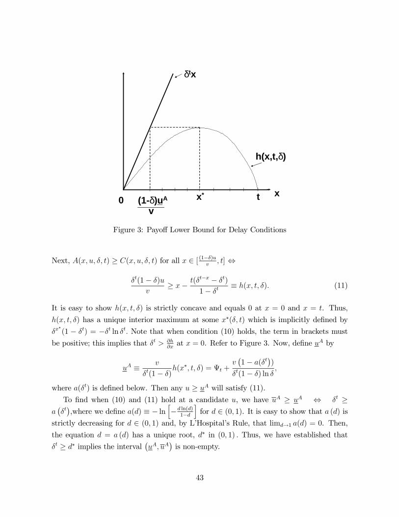
x

δtx

h(x,t,δ)

x*(1­δ)uA

v0 t

Figure 3: Payo¤ Lower Bound for Delay Conditions

Next, A(x; u; �; t) � C(x; u; �; t) for all x 2 [ (1��)uv

; t] ,

�t(1� �)u

v� x� t(�t�x � �t)

1� �t� h(x; t; �): (11)

It is easy to show h(x; t; �) is strictly concave and equals 0 at x = 0 and x = t. Thus,

h(x; t; �) has a unique interior maximum at some x�(�; t) which is implicitly de�ned by

�x�(1 � �t) = ��t ln �t: Note that when condition (10) holds, the term in brackets must

be positive; this implies that �t > @h@xat x = 0. Refer to Figure 3. Now, de�ne uA by

uA � v

�t(1� �)h(x�; t; �) = t +

v�1� a(�t

�)

�t(1� �) ln �;

where a(�t) is de�ned below. Then any u � uA will satisfy (11).

To �nd when (10) and (11) hold at a candidate u, we have uA � uA , �t �a��t�,where we de�ne a(d) � � ln

h�d ln(d)

1�d

ifor d 2 (0; 1). It is easy to show that a (d) is

strictly decreasing for d 2 (0; 1) and, by L�Hospital�s Rule, that limd!1 a(d) = 0. Then,

the equation d = a (d) has a unique root, d� in (0; 1) : Thus, we have established that

�t � d� implies the interval�uA; uA

�is non-empty.

43

The last step of the proof is to consider the range of values for u that can be supported.

A straightforward argument establishes that uA < vt1�� holds for �

t � d�. The comparison

of uA with vt1�� reveals that u

A crosses vt1�� exactly one time, from below, at the root of the

equation � ln �t = (��t � 1)2; numerically, the root is :572, which exceeds d�. Thus, for�t below this root, we have uA < vt

1�� and any u 2�uA; uA

�satis�es the delay condition

(5). For �t above this root, we have uA > vt1�� > uA and there are two cases. First, by the

above analysis, any u 2�uA; vt

1���satis�es the delay condition (5). Second, for the case

of u 2�vt1�� ; u

A�, the delay condition (5) requires that A(x; u; �; t) � B(x; �; t) for all x in

the interval [0; t]; note that since u is large, the case of (1��)uv

< x � t never arises. Then

A(x; u; �; t) � B(x; �; t) and utilities in this payo¤ range satisfy (5). �(iii) O¤ Equilibrium Support (Cash-in o¤ers)

Now, we deal with o¤ equilibrium states (� ; 0) where � > t. Since we are using cash-in

supports, the payo¤s are �� = p� + ��1 for the seller and u� = v� � p� + �u(� + 1; �) =v�1�� � p� + �u1 for buyers. Note that from (� ; 0) the surplus on the continuation path is

� �v�

1� �+ �1 = �� + u� for � > t

and that cash-in states contrast with delay states, � < t, where we have � � �t��t:

Recall from the text that we must satisfy (1) and (2). Thus, we seek a utility sequence

that satis�es the analog of (3), as given by

� � ��+1�� � u� � �u�+1�� + g(�; u�+1) (12)

for � � t and � = 0; :::; � . Analogous to our support utility sequence for e¢ cient equilibria,

we de�ne a T � stage support sequence, where T � t+ 1, for ine¢ cient equilibria by

u� =

(�u�+1 +� � ��+1 for � = 1; :::; T � 1uT for � � T:

For the special case of T = t, we specify a constant sequence u� = ut for all � . As before,

the seller is indi¤erent with respect to delay and the cash-in up to state T , and the seller

prefers to cash-in in state T provided that the buyers�utilities, uT , are not too large.

We can satisfy (12) by an appropriate choice of the support length T for a given �

and buyer payo¤. Recalling Figure 1 for e¢ cient equilibria, we �nd a similar structure

for the relationship between ut, �, and the length of a T . For any given � we can support

successively higher buyer payo¤s by increasing the support horizon, T . In particular as

44

ut rises, then T must also rise until we achieve ut 2 [t � �T�tS1;t � �T�t+1S1]. Thus,

Lemma A6 Let T � t and suppose �+ �T � 1. Let buyer utilities follow a T � stagesupport, where ut satis�es (i) 0 � ut � t � �S1 for T = t and (ii) t � �T�tS1 � ut �t � �T�t+1S1 for T > t. Then (12) holds for every � � t and � = 0; :::; � :

(iv) Equilibrium Existence

The following lemma provides su¢ cient conditions for equilibrium existence.

Lemma A7 Suppose a sequence of buyer utilities u� satis�es (5) and (12) for somet � 2 and for all � and � , such that 0 � � � � for any � � 1: Then there exists an

ine¢ cient t� cycle equilibrium with a buyer payo¤ of u1.

Proof. The delay conditions are satis�ed by Lemma 4 for ut 2�uA; uA

�. With (12)

satis�ed as well, we know that no single-bundle deviation is pro�table for the seller. As

with the e¢ cient case, we must now show that the seller cannot pro�tably deviate to

an upgrade o¤er set in state � . While the logic is similar to that for e¢ cient equilibria,

the proof is more complicated and we only provide a brief sketch. We must distinguish

between delay states, where � < t, and support states where � � t. We de�ne a BCE

based on the same buyer preference relation �B but now u(� + 1; b) and u(� + 1; b j i)must account for whether there is a delay or a cash-in the continuation state. We can

then show the same argmax construction yields a BCE. Next, note that any upgrade o¤er

can be written in the form B = I [ J [ K where an upgrade to b is in I if pb � Gb, in

J if pb � Hb, and in K if Gb < pb < Hb. The threshold prices, following the buyer and

seller decisions in the text at (12), are speci�ed by

Gb =

(vb1��

�1� �t��

�+ �t�� max

�vb1�� ; ut

� �t��ut if � < t

vb+ �max�vb1�� ; u�+1

� �u�+1 if � � t

and

Hb =

(�t��

�1� �b

�( t � ut) if � < t

( � � u� )� �� �+1�b � u�+1�b

�if � � t

:

The proof then proceeds by considering the various cases for the decomposition B =I [ J [ K. For instance, if J is empty then we are done as the argmax property can be

applied to I [ K and we can specify that buyers choose this BCE, which is priced belowHb. The most di¢ cult case arises when none of the component sets in I [J [K is empty.We can show that there always exists a BCE priced below Hb in this case.

The next step is to specify continuation equilibrium strategies at asymmetric buyer

states, (� ; �); see part (i) of Appendix B for the de�nition. These states are complicated

45

by the fact that joint surplus is not maximized in an ine¢ cient t�cycle equilibrium. Thiscontrasts with the e¢ cient case, where the (� ; �) o¤ers fully extracted buyers relative to

equilibrium payo¤s for the continuation state of (� + 1; �) ; since feasibility will no longer

imply this is an optimal o¤er for the seller. Instead, we specify a continuation equilibrium

that leaves buyers asymmetric. Thus, this part of the support neither returns to the

equilibrium path nor to a cash-in support state.

Let �m � inf f�� j �� > 0; g denote the smallest non-zero mass of buyers in � andif the inf is not unique let m be the largest index (e.g., if �� = 1=� for all � then

�m = 1=� and m = � � 1). We specify that the seller o¤ers a collection of upgradesf(b�; p�)g�=0;:::;��1with prices of

pm =v (� � 1�m)

1� �; and p� =

v (� � �)

1� �for � 6= m:

It is straightforward to verify that all buyers optimally accept and that the continua-

tion state is of the form (� + 1; �0) where �0 = (0; :::; 0; �m; 1� �m). Thus, in the state for

period � +1 the smallest mass group is at quality level � � 1 units, while all other buyersare at � . We then apply the same logic to specify o¤ers for (� + 1; �0) and all resulting

states so that the distribution of buyers is always concentrated in the same proportions

(�m; 1� �m) at the two highest quality levels.

The argument that this is an optimal strategy for the seller is involved, so we only

o¤er a brief sketch. For any arbitrary seller o¤er in (� ; �) and pattern of buyer choices,

one can bound the seller payo¤ via individual rationality of the buyer choices, using

the hypothesis that the seller makes the o¤er in the continuation state in period � + 1

that induces a concentration of buyers at the two highest quality levels (if the buyer

choices lead to a degenerate distribution, then payo¤s must instead follow the t � cycle

equilibrium path and cash-in support). Then, since the repeated concentration of buyers

in proportions (�m; 1� �m) at the two highest quality levels allows the seller to extract

all surplus generated on this path, the associated seller payo¤ can be shown to be at least

as large as the bound derived from individual buyer rationality for any other seller o¤er.

In this regard, note that every equilibrium with delay (t � 2) has a buyer quality level

that is strictly below the mean for the (�m; 1� �m) concentration.

Finally, �nding a BCE for an arbitrary upgrade o¤er B in state (� ; �) follows the samebasic logic as that for an e¢ cient equilibrium. The only di¤erence is that we must take

care to account for any possible delay if the continuation state is degenerate. �

46

Proof of Proposition 4. De�ne �(t; T; �) � t � �T�tS1, the upper bound on payo¤s

that can be supported with a T � stage support: We claim �(t; T; �) � uA(t; �) holds

whenever � satis�es the delay conditions. Comparing, �(t; T; �) � uA(t; �),

(1� �t)(1� �)

�T� � ln � (13)

It is clear that both sides of (13) are positive, falling in � and equal to 0 at � = 1. The

l.h.s. of (13) is rising in T and t. Di¤erentiating both sides of (13) with respect to � we

�nd that the slope of the l.h.s. is greater/less than the slope of the r.h.s. if and only if

�T + �t+1 ? T (1� �) + � � (T � t)�t(1� �) (14)

In (14), the l.h.s. is positive and convex in � and the r.h.s. is decreasing in �. Thus, the

l.h.s. and the r.h.s. of (13) cross a single time in �. It easy to see that (13) is negative in a

neighborhood of 1 and positive at � = tpd� for any T � t. So, there is a (t; T ) 2 ( t

pd�; 1)

such that (13) holds whenever � � (t; T ). Clearly, (t; T ) is increasing in T .

Now, we will show that (t; T ) > �T for all t � 2: At = (t; T ) we have

1�

T=� ln 1� t

The r.h.s. is falling in . Since for any this is less than 1, (t; T ) > �T . �

47