QTune: A Query-Aware Database Tuning System with DeepReinforcement Learning

Guoliang Li†, Xuanhe Zhou†, Shifu Li‡, Bo Gao‡† Department of Computer Science,Tsinghua University, Beijing, China ‡ Huawei Company

liguoliang@tsinghua.edu.cn, zhouxuanhe@bupt.edu.cn, {gaobo15,lishifu}@huawei.com

ABSTRACTDatabase knob tuning is important to achieve high perfor-mance (e.g., high throughput and low latency). However,knob tuning is an NP-hard problem and existing methodshave several limitations. First, DBAs cannot tune a lot ofdatabase instances on different environments (e.g., differ-ent database vendors). Second, traditional machine-learningmethods either cannot find good configurations or rely on alot of high-quality training examples which are rather hardto obtain. Third, they only support coarse-grained tuning(e.g., workload-level tuning) but cannot provide fine-grainedtuning (e.g., query-level tuning).

To address these problems, we propose a query-awaredatabase tuning system QTune with a deep reinforcementlearning (DRL) model, which can efficiently and effectivelytune the database configurations. QTune first featurizes theSQL queries by considering rich features of the SQL queries.Then QTune feeds the query features into the DRL model tochoose suitable configurations. We propose a Double-StateDeep Deterministic Policy Gradient (DS-DDPG) model toenable query-aware database configuration tuning, whichutilizes the actor-critic networks to tune the database config-urations based on both the query vector and database states.QTune provides three database tuning granularities: query-level, workload-level, and cluster-level tuning. We deployedour techniques onto three real database systems, and exper-imental results show that QTune achieves high performanceand outperforms the state-of-the-art tuning methods.

PVLDB Reference Format:Guoliang Li, Xuanhe Zhou, Shifu Li, Bo Gao. QTune: A Query-Aware Database Tuning System with Deep Reinforcement Learn-ing. PVLDB, 12(12): 2118 - 2130, 2019.DOI: https://doi.org/10.14778/3352063.3352129

1. INTRODUCTIONDatabases have hundreds of knobs (or parameters) and

most of knobs are in continuous space. For example, MySQL,PostgreSQL, and MongoDB have 215, 247, 132 knobs re-spectively. Database knob tuning is important to achieve

This work is licensed under the Creative Commons Attribution-NonCommercial-NoDerivatives 4.0 International License. To view a copyof this license, visit http://creativecommons.org/licenses/by-nc-nd/4.0/. Forany use beyond those covered by this license, obtain permission by emailinginfo@vldb.org. Copyright is held by the owner/author(s). Publication rightslicensed to the VLDB Endowment.Proceedings of the VLDB Endowment, Vol. 12, No. 12ISSN 2150-8097.DOI: https://doi.org/10.14778/3352063.3352129

high performance (e.g., high throughput and low latency) [2,5, 34]. Traditionally, databases rely on DBAs to tune theknobs. However, this traditional method has several limita-tions. First, knob tuning is an NP-hard problem [27] andDBAs can only tune a small percentage of the knobs andmay not find a good global knob configuration. Second,DBAs require to spend a lot of time (e.g., several days)to tune the database, and thus they are not efficient totune many database instances under different environments(e.g., cloud databases). Third, DBAs are usually good attuning a specific database, e.g., MySQL, but cannot tuneother databases, e.g., PostgreSQL. These limitations are ex-tremely severe for tuning cloud databases, because they haveto tune a lot of database instances on different environments(e.g., different CPU, RAM and disk).

Recently, there are some studies on automatic knob tun-ing, e.g., BestConfig [38], OtterTune [2], and CDBTune [36].However, BestConfig uses a heuristic method to search forthe optimal configuration from the history and may not findgood knob values if there is no similar configuration in thehistory. OtterTune utilizes machine-learning techniques tocollect, process and analyze knobs and tunes the database bylearning DBAs’ experiences from the historical data. How-ever, OtterTune relies on a large number of high-qualitytraining examples from DBAs’ experience data, which arerather hard to obtain. CDBTune uses deep reinforcementlearning (DRL) to tune the database by using a try-and-error strategy. However, CDBTune has three limitations.First, CDBTune requires to run a SQL query workload mul-tiple times in the database to get an appropriate configu-ration, which is rather time consuming. Second, CDBTuneonly provides a coarse-grained tuning (i.e., tuning for read-only workload, read-write workload, write-only workload),but cannot provide a fine-grained tuning (i.e., tuning for aspecific query workload). Third, it directly uses the existingDRL model, which assumes that the environment can onlybe affected by reconfiguring actions, but cannot utilize thequery information, which is more important for configura-tion tuning and environment updates.

To address these problems, we propose a query-awaredatabase tuning system QTune using a DRL model, whichcan efficiently and effectively tune the databases. QTune

first featurizes the SQL queries by considering rich featuresof the SQL queries, including query type, tables, and querycost. Then QTune feeds the query features into the DRLmodel to dynamically choose suitable configurations. Dif-ferent from the traditional DRL methods [16, 30], we pro-pose a Double-State Deep Deterministic Policy Gradient

2118

(DS-DDPG) model using the actor-critic networks. TheDS-DDPG model can automatically solve the tuning prob-lem by learning the actor-critic policy according to both thedatabase states and query information. Moreover, QTune

provides three database tuning granularities. The first isquery-level tuning, which finds a good configuration for eachSQL query. This method can achieve low latency but lowthroughput, because it cannot run the SQL queries in par-allel. The second is workload-level tuning, which finds agood configuration for a query workload. This method canachieve high throughput but high latency, because it cannotfind a good configuration for every SQL query. The thirdis cluster-level tuning, which clusters the queries into sev-eral groups and finds a good database configuration for thequeries in each group. This method can achieve both highthroughput and low latency, because it can find the goodconfiguration for a group of queries and run the queriesin each group in parallel. Thus QTune can make a trade-off between latency and throughput based on a given re-quirement, and provide both coarse-grained tuning and fine-grained tuning. We propose a deep learning based queryclustering method to classify queries according to the simi-larity of their suitable configurations.

We make the following contributions in this paper.(1) We propose a query-aware database tuning system usingdeep reinforcement learning, which provides three databasetuning granularities (see Section 2).(2) We propose a SQL query featurization model that fea-turizes a SQL query to a vector by using rich SQL features(see Section 3).(3) We propose the DS-DDPG model, which embeds thequery features and utilizes the actor-critic algorithm to learnthe relations among queries, database state and configura-tions to tune database configurations (see Section 4).(4) We propose a deep learning based query clustering methodto classify queries according to the similarity of their suit-able configurations (see Section 5).(5) We conducted extensive experiments on various queryworkloads and databases. Experimental results showed thatQTune achieved high performance and outperformed the state-of-the-art tuning methods (see Section 6).

2. SYSTEM OVERVIEWIn this section, we present the system overview of QTune.

QTune supports three types of tuning requests based on dif-ferent tuning granularities.

Query-level Tuning. For each query, it first tunes thedatabase knobs and then executes the query. Note thatthe session-level knobs (e.g., bulk write size) can be con-currently tuned for different queries, while the system-levelknobs (e.g., working memory size) cannot be concurrentlytuned because when we tune these knobs for a query, thesystem cannot process other queries. This method can op-timize the latency but may not achieve high throughput.

Workload-level Tuning. It tunes the database knobs forthe whole query workload. This method cannot optimizethe query latency, because different queries may require touse different best knob values. This method, however, canachieve high throughput, because different queries can beconcurrently processed after setting the newly tuned knobs.

Cluster-level Tuning. It partitions the queries into differ-ent groups such that the queries in the same group shoulduse the same tuning knob values while the queries in differ-

`

Figure 1: The QTune Architectureent groups should use different knob values. Next it tunesthe knobs for each query group and executes the queries ineach group in parallel. This method can optimize both thelatency and throughput.

Architecture. Figure 1 shows the architecture of QTune,which contains five main components. Figure 2 shows theworkflow. The client interacts with Controller to pose tun-ing requests. Query2Vector featurizes each query into a vec-tor. It first analyzes the SQL query, extracts the query planand the estimated cost of each query from the database en-gine, and uses this information to generate a vector. Basedon the feature vectors, Tuner recommends appropriate knobsand then the database executes these queries based on thenew knob values. Tuner uses the deep reinforcement modelDS-DDPG to tune the model and recommend continuousknob values as a new configuration. Tuner also requires totrain the model using some training data, which is stored inthe Training Data repository. We will explain more detailsof Tuner in Section 4.

For query-level tuning, Query2Vector generates a featurevector for the given query. Tuner takes this vector as input,and recommends continuous knob values. Next the systemexecutes the query based on the recommended knob values.

For workload-level tuning, Query2Vector generates a fea-ture vector for each query in the workload and merges themto generate a unified vector. Tuner takes this unified vec-tor as input, and recommends knob values. Next the systemexecutes the queries based on the recommended knob values.

For cluster-level tuning, Query2Vector first generates afeature vector for each query and Tuner learns a configura-tion pattern for each query which can learn the continuousknob values that best match the query. However, Tuner

may be expensive to generate the configuration pattern forall the queries. To improve the performance, we propose adeep learning model, Vector2Pattern, which learns a dis-crete value for the knobs. Then Pattern2Cluster classi-fies these queries based on their discrete configuration pat-terns. Note that Vector2Pattern uses deep learning to pre-dict the configuration pattern for each query, which alsoinvolves a training step that learns a discrete configurationpattern for a given query. For example, considering the knobhost cache size in MySQL, which limits the size of the hostcache, Tuner recommends a continuous value between 0 to65536, while Vector2Pattern recommends a discrete valuein {-1, 0, +1}. After clustering, we get a set of groups. Foreach query group, Tuner recommends appropriate configu-rations and then the database executes these queries in thegroup based on the new knob values. So in Figure 2, weprovide two cluster-level algorithms. Cluster-level(C) usesthe DRL model to learn continuous values while Cluster-level(D) uses the DL model to learn discrete values.

3. QUERY FEATURIZATIONIn this section we introduce how to vectorize the queries.

There are several challenges in query featurization. The

2119

Queries

Q = {Q1, Q2, ..., Qn}

Configuration

Figure 2: Workflow of QTune

first is to capture the query information, e.g., which tablesare involved in the query. The second is to capture thequery cost of processing the query, e.g., the selection costand join cost. The third is to uniformly featurize the queryand cost information such that each feature of the vectorfor different queries has the same meaning. Next we discusshow to address these challenges in the following sections.

3.1 Query InformationA SQL query includes query type (e.g., insert, delete, se-

lect, update), tables, attributes, operations (e.g., selection,join, groupby). Query type is important as different querytypes have different query cost (e.g, OLTP and OLAP havedifferent effect on the database), and thus we need to capturethe query type information in the vector. Tables involved ina query are also important, because the data volumes andstructures of tables will significantly affect the database per-formance. Based on the table information, our tuning modeldecides whether the current system configuration can pro-vide high performance; if not, our tuning system can tunethe corresponding knobs. For example, if the buffer is notlarge enough, we can increase the buffer.

Note that we do not featurize the attributes (i.e., columns)and operations (i.e., selection conditions) due to three rea-sons. First, the query cost will capture the operation infor-mation and cost, and we do not need to maintain duplicatedinformation. Second, operations are too specific and addingspecific operations into the vectors will reduce the general-ization ability. Third, the attributes and operations will befrequently updated and it requires to redesign the model forthe updates. We will compare with the method that alsoconsiders attributes and operations in Section 6.1.2 .

In summary, for query information, we maintain a 4 + |T |dimensional vector, where |T | is the number of tables in thedatabase. The first four features capture the query types,e.g., insert, select, update, delete. For an insert/select/up-

date/delete query, the corresponding value is 1; 0 otherwise.Each last |T | feature denotes a table. If the query containsthe table, the corresponding value is 1; 0 otherwise. For ex-ample, Figure 3 shows a query vector. There are 8 tables.The first 12 features are used for query information. It is aselection query and uses tbl1, tbl2 and tbl3, so the first fourvalues are 1 and the other 8 values are 0.

3.2 Cost InformationThe cost information captures the cost of processing the

query. However, a query usually has many possible phys-ical plans and each plan has different query cost. So it isnot realistic to directly parse the query statement to extractquery cost. Instead, we utilize the query plan generated bythe query optimizer, which has a cost estimation for each op-eration. Figure 3 shows an example query plan, where eachnode has a cost estimation. As each database has a fixednumber of operations, e.g., scan, hash join, aggregate, we usethe cost on these operations to capture the cost information.For example, in PostgreSQL there are 38 operations. Notethat an operation may appear in different nodes of the treeplan, and the cost of the same operation should be summedup as the corresponding cost value in the query cost vector.For example, in Figure 3, the value of hash join equals to thesum of the costs in the two Hash Join nodes. After gainingthe query cost, we normalize the cost by subtracting meanand dividing the std deviation.

In summary, for cost information, we maintain a |P | di-mensional vector, where P is the set of operations in database,and |P | is the number of operations.

3.3 Character EncodingWe concatenate the query vector and cost vector to gen-

erate an overall vector of a query. For example, Figure 3shows the vector of a SQL query.

2120

tbl1.info = '%act%'

Total17.8

Startup0

Child 0

tbl3

tbl1.id = tbl3.type_idtbl2

tbl2.movie_id = tbl3.movie_id

MIN(tbl3.movie_id)

0 0

2.430

23.24

Seq Scan

Total2.41

Startup0

Child 0

Seq Scan

Total 23.19

Startup2.43

Child 0

Hash Join

Total 20.7

Startup0

Child 0

Seq Scan

Total48.16

Startup23.24

Child 2.43

Hash Join

Total 48.28

Startup48.27

Child 23.24

Aggregate

Insert Delete Update Select tbl1 tbl2 tbl3 ... tbl8 Hash_Join Seq_Scan Aggregate ...

[ 0 0 0 1 1 1 1 ... 0 68.92 40.91 25.04 ... ]

Insert Delete Update Select tbl1 tbl2 tbl3 ... tbl8 Hash_Join Seq_Scan Aggregate ...

[ 0 0 0 1 1 1 1 ... 0 0.1401 -0.166 -0.2423 ... ]

(1) DML (2) Tables (3) Operation Costs

Normalized Feature Vector

FROM tbl1, tbl2, tbl3

WHERE tbl1.info = '%act%'

AND tbl1.id = tbl3.type_id

AND tbl2.movie_id = tbl3.movie_id

SELECT MIN(tbl3.movie_id)

Figure 3: Character Encoding.Vector for multiple queries. Given multiple queriesq1, q2, · · · , qm, suppose their vectors are v1, v2, · · · , vm re-spectively. To tune the database for this query workload,we need to combine the vectors together. To this end, foreach query vector, we need to consider all the query typesand tables, and thus we compute the union of the query vec-tors. And for each table, if the value is 1, we replace it withthe row number of the table. Thus it can capture the actionslike deleting/inserting rows and improve system’s adaptiv-ity; for cost vector, we need to sum up all the costs. Thuswe can combine the vector as follows.

[∪m1 vi[1], . . . ,∪m1 vi[4+|T |],∑m

1 vi[5+|T |], · · · ,∑m

1 vi[4+|T |+|P |]]Supporting Update. We discuss how to support the up-date of the databases. The database update can only affectthe query vector, as the cost vector is computed on-the-flyfrom the optimizer, which can get the updated cost. Forquery vector, only adding/removing tables will affect thequery vector. To this end, we can leave several positions forcapturing future updates of adding/deleting tables.

4. DRL FOR KNOB TUNINGSince there are hundreds of knobs in a database and many

of them are in continuous space [5], the database tuningproblem is NP hard and it is rather expensive to find high-quality configurations [34]. We utilize the deep reinforce-ment learning model, which combines reinforcement learn-ing and neural networks to automatically learn the knobvalues from limited samples. Note that existing DRL mod-els [16, 19, 12] cannot utilize the query features as theyignore the effects to the environment state from the query,and we propose a Double-State Deep Deterministic PolicyGradient (DS-DDPG) model to enable query-aware tuning.

4.1 DS-DDPG ModelThe DS-DDPG model contains five components as shown

in Figure 4. Table 1 shows the mapping from the DS-DDPG

Figure 4: The DS-DDPG Model

Table 1: Mapping from DS-DDPG to Tuning

DS-DDPG The tuning problemEnvironment Database being tunedInner state Database knobs (e.g., work mem)

Outer metrics State statistics (e.g., updated tuples)Action Tuning database knobsReward Database performance changesAgent The Actor-Critic networks

Predictor A neural network for predicting metricsActor A neural network for making actionsCritic A neural network for evaluating Actor

model to the tuning problem. Environment contains thedatabase information, which includes the inner state and theouter metrics. The inner state records the database config-uration (i.e., knob configurations) which can be tuned, andthe outer metrics record the state statistics (e.g., databasekey performance indicators), which reflect database statusand cannot be tuned. For example, in PostgreSQL theinner state includes working memory, effective cache size,etc, and the outer metrics include the number of committedtransactions, the number of deadlocks, etc. Query2Vector

generates the feature vector for a given query (or a work-load). Predictor is a deep neural network, which predictsthe changes in outer metrics of before/after processing thequeries. We predict ∆S because most of the outer metricsare accumulative variables (others are related to the systemperformance, such as the time to read a block) and theirdifference in values can reflect the workload’s effect to thedatabase state. Besides, predicting ∆S is much easier thanS′, as S′ is not only related to the workload features, but cur-rent database state. Environment combines these changes∆S with its original metrics S and generates the observationS′ = S + ∆S to simulate the outer metrics after executingthe queries. Agent is used to tune the inner state basedon the observation S′. Agent contains two modules, Actorand Critic, which are two independent neural networks.Actor takes S′ as input, and outputs an action (a vectorof tuned knob configurations). Environment executes thequery workload and computes a reward based on the perfor-mance. Critic takes the observation S′ and the action asinput, and outputs a score (Q-value), which reflects whetherthe action tuning is effective. Critic updates the weights ofits neural network based on the reward value. Actor updatesthe weights of its neural network based on the Q-value. So

2121

Actor generates a tuning action and Environment deploysthe tuning action and generates a reward value based on theperformance change on the new configuration. If the per-formance change is positive, it will return a positive reward;negative otherwise. Critic updates the network based onthe reward. The five components work together and canautomatically recommend good configurations.

DS-DDPG is an effective strategy to solve optimal prob-lems with continuous action space by concurrently learningthe Q-value function and the action policy. When the num-ber of actions is finite, we can compute each action’s Q-valueand choose the action with maximal Q-value. But in contin-uous space, this method such as Q-learning does not work,because it’s impossible to exhaustively search the space. In-stead, in DDPG, we train two neural networks to adapt tocontinuous action space: the Critic network can give theQ-value for each 〈observation, action〉 and the Actor net-work updates its action policy based on the Q-value andchooses proper action according to the observation. Sinceneural network can perform well in high-dimensional datamapping with proper architecture design and training, DS-DDPG can also handle problems with high-dimensional in-put/output data. In the database tuning problem, we needto tune many knobs which are in continuous space, and thusDS-DDPG is suitable for this problem.

4.2 Training DS-DDPGWe discuss how to train the DS-DDPG model (Predictor,

Actor and Critic), and Algorithm 1 shows the pseudo code.

4.2.1 Training the PredictorTraining Data TP . Predictor aims to predict the databasemetrics change if processing a query in the database. Thetraining data is a set of tuples TP = {〈v, S, I,∆S〉}, wherev is a vector of a query, S is the outer metrics, I is the innerstate and ∆S is the outer metrics change by processing v ina database. For each 〈v, S, I〉, we train Predictor to outputa value that is close to ∆S.

The training data can be easily obtained as follows. Givena query workload, for each query q, we first use Query2Vectorto generate v and obtain metrics S and state I from theEnvironment. Then we run q in the database and recordthe metrics change ∆S.

Training. Predictor is a multilayer perceptron model,which is composed of four fully connected layers: the inputlayer accepts the feature vector and outputs the mappedtensor (higher dimensions) to the hidden layers. These twohidden layers have a series of non-linear data transforma-tions. The output restricts the tensor to the scale of thedatabase state and generates a vector representing the pre-dicted database metrics changes. The network actually rep-resents a chain of function compositions which transformthe input to the output space (a pattern) [6]. To avoid ournetwork model from just learning in linear transformations,we add ReLU (a type of activation function most commonlyused in neural network [1]) to the hidden layers to capturemore complicated patterns. The weights in the network areinitialized by the standard normal distribution.

Given a training dataset {(v1, S1, I1,∆S1), . . .}, the train-ing target is to minimize the error function, defined as

E =1

2

|U|∑i=1

||Gi −∆Si||2 . (1)

Algorithm 1: Training DS-DDPG

Input: U: the query set {q1, q2, · · · , q|U|}Output: πP , πA, πC

1 Generate training data TP ;2 TrainPredictor(πP , TP );3 Generate training data TA;4 TrainAgent(πA, πC , TA);

Function TrainPredictor(πP , TP )

Input: πP : The weights of a neural network; TP :The training set

1 Initiate the weights in πP ;2 while !converged do3 for each (v, S, I,∆S) ∈ TP do4 Generate the output G of 〈v, S, I〉;5 Accumulate the backward propagation error:

E = E + 12||G−∆S||2;

6 Compute gradient ∇θs(E), update weights in πP ;

Function TrainAgent(πA, πC , TA)

Input: πA: The actor’s policy; πC : The critic’spolicy; TA: training data

1 Initialize the actor πA and the critic πC ;2 while !converged do3 Get a training data

T 1A = (S′1, A1, R1), (S′2, A2, R2), . . . , (S′t, At, Rt);

4 for i = t− 1 to 1 do5 Update the weights in πA with the

action-value Q(S′i, Ai|πC);6 Estimate an action-value

Yi = Ri + τQ(S′i+1, πA(S′i+1|θπA)|πC);7 Update the weights in πC by minimizing the

loss value L = (Q(S′i, At|πC)− Yi)2;

where Gi is the output value by Predictor for query qi, andU is the query set.

We adopt Adam [10] to train Predictor. Adam is astochastic optimization algorithm. It iteratively updates thenetwork weights by the first and second moments of the gra-dients, which are computed using stochastic objective func-tion. The training procedure terminates if the model is con-verged or runs a given number of steps.

4.2.2 Training the Actor-Critic ModuleTraining Data TA. The agent (i.e., the Actor-Critic mod-ule) aims to judiciously tune the database configurations.Given a query workload, we randomly select a subset ofqueries and generate a sample workload. For the samplequery workload, we generate its feature vector via Query2Vector,predict a database metrics S′1 via Predictor, get an actionA1 via Actor, deploy the actions in the databases, run thedatabase to get a reward R1 (the reward function will bediscussed later). In the next step, we get a new databasemetrics S′2 by updating S′1 using the new metrics, and repeatthe above steps to get A2 and R2. Iteratively, we get a set oftriples 〈T 1

A = (S′1, A1, R1), (S′2, A2, R2), . . . , (S′t, At, Rt)〉 un-til the average reward value is good enough (e.g., the averagereward of ten runs is larger than 10.)

Training Actor and Critic. The training of the Actor-Critic module is to update the weights in their neural net-

2122

works. We first initiate the DS-DDPG model, including theenvironment, the actor policy πA and the critic policy πC .Then we use the experience replay method to train the actorand the critic in the reinforcement learning process.

Given a training dataset 〈T 1A = (S′1, A1, R1), (S′2, A2, R2), . . .,

(S′t, At, Rt)〉, we consider (S′i, Ai, Ri) and update Actor andCritic as follows.

(1) We update the actor policy πA using the gradient value

∇θπAπA = ∇AiQ(S′i, Ai|πC) · ∇θπAπA(S′i|θπA)

where θ is the parameters in πA and Q(S′i, Ai|πC) is theQ-value computed by Critic.

(2) We estimate the real action-value Yi. We use the Bell-man function [32] to compute Yi based on the reward andQ-value, i.e.,

Yi = Ri + τ ·Q(S′i+1, πA(S′i+1|θπA)|πC)

where τ is a tuning factor to tradeoff the Q-value and thereward value.

(3) We calculate the loss value L with Q and Y . Critic

updates the weights in πC by minimizing the loss value

L = (Q(S′i, Ai|πC)− Yi)2

We run the three steps for i = t− 1 to i = 1.The algorithm terminates if the model is converged (e.g.,

the performance improvement is smaller than a threshold);otherwise we select next training data T 2

A, T3A, · · · .

Target network. To improve the stability of training, wecan introduce two extra target actor and critic networks(whose policies are π′A and π′C respectively). These twonetworks are updated at every step and their weights (pa-rameters of the policy) are updated slower than the normalnetworks. Then the weights in the normal critic network areupdated by minimizing loss compared with the target:

L(πC) = (Q(S′i, Ai|πC)− Yi)2

Yi = Ri + τ ·Q(S′i+1, π′A(S′i+1|θπ

′A)|π′C)

Reward Function. Our reward function is designed tocapture two abilities. 1) It can provide valuable feedbackof the database performance; 2) It takes multiple metricsinto consideration, and each metric can have different im-portance by assigning different weights.Step 1. For each metric m, e.g., latency and throughput,calculate the performance change compared with that atinitial time (∆0,t) and that at last time (∆t−1,t).

∆0,t =

{mt−m0m0

, the higher the betterm0−mtm0

, the lower the better

∆t−1,t =

{mt−mt−1

mt−1, the higher the better

mt−1−mtmt−1

, the lower the better

Step 2. The reward function of metric m is designed as:

rm =

{((1 + ∆t−1,t)

2 − 1)|1 + ∆0,t|, ∆0,t > 0

−(((1−∆t−1,t)2 − 1)|1−∆0,t|), ∆0,t ≤ 0

Step 3. The reward function R on multiple metrics is

R =∑

wmrm

where wm is the weight manually assigned for metric m.

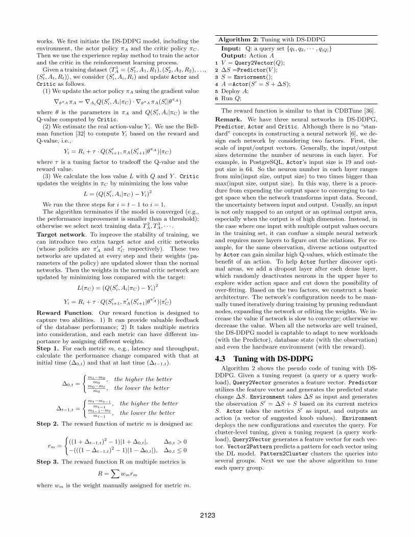
Algorithm 2: Tuning with DS-DDPG

Input: Q: a query set {q1, q2, · · · , q|Q|}Output: Action A

1 V = Query2Vector(Q);2 ∆S =Predictor(V );3 S = Enviorment();4 A =Actor(S′ = S + ∆S);5 Deploy A;6 Run Q;

The reward function is similar to that in CDBTune [36].

Remark. We have three neural networks in DS-DDPG,Predictor, Actor and Critic. Although there is no “stan-dard” concepts in constructing a neural network [6], we de-sign each network by considering two factors. First, thescale of input/output vectors. Generally, the input/outputsizes determine the number of neurons in each layer. Forexample, in PostgreSQL, Actor’s input size is 19 and out-put size is 64. So the neuron number in each layer rangesfrom min(input size, output size) to two times bigger thanmax(input size, output size). In this way, there is a proce-dure from expending the output space to converging to tar-get space when the network transforms input data. Second,the uncertainty between input and output. Usually, an inputis not only mapped to an output or an optimal output area,especially when the output is of high dimension. Instead, inthe case where one input with multiple output values occursin the training set, it can confuse a simple neural networkand requires more layers to figure out the relations. For ex-ample, for the same observation, diverse actions outputtedby Actor can gain similar high Q-values, which estimate thebenefit of an action. To help Actor further discover opti-mal areas, we add a dropout layer after each dense layer,which randomly deactivates neurons in the upper layer toexplore wider action space and cut down the possibility ofover-fitting. Based on the two factors, we construct a basicarchitecture. The network’s configuration needs to be man-ually tuned iteratively during training by pruning redundantnodes, expanding the network or editing the weights. We in-crease the value if network is slow to converge; otherwise wedecrease the value. When all the networks are well trained,the DS-DDPG model is captable to adapt to new workloads(with the Predictor), database state (with the observation)and even the hardware environment (with the reward).

4.3 Tuning with DS-DDPGAlgorithm 2 shows the pseudo code of tuning with DS-

DDPG. Given a tuning request (a query or a query work-load), Query2Vector generates a feature vector. Predictor

utilizes the feature vector and generates the predicted statechange ∆S. Environment takes ∆S as input and generatesthe observation S′ = ∆S + S based on its current metricsS. Actor takes the metrics S′ as input, and outputs anaction (a vector of suggested knob values). Environment

deploys the new configurations and executes the query. Forcluster-level tuning, given a tuning request (a query work-load), Query2Vector generates a feature vector for each vec-tor. Vector2Pattern predicts a pattern for each vector usingthe DL model. Pattern2Cluster clusters the queries intoseveral groups. Next we use the above algorithm to tuneeach query group.

2123

5. QUERY CLUSTERINGFor workloads including both transactional queries and

analytical queries [25], if the user aims to optimize the la-tency, we recommend query-level tuning; if the user aimsto improve the throughput, we recommend workload-leveltuning. For analytical only queries, we recommend cluster-level tuning to balance the throughput and latency. Thekey problem in the cluster-level tuning is (1) how to effi-ciently find the appropriate configuration pattern for eachquery and (2) how to cluster the queries based on the con-figuration pattern. This section studies these two problems.

5.1 Configuration PatternThe configuration pattern of a query should include all

the knobs used in the DS-DDPG model. Thus a natureidea is to use DS-DDPG to generate a continuous knob con-figuration and take the knob configuration as the pattern.However it is rather expensive to get the continuous knobvalues, especially for a large number of queries. More im-portantly, when we cluster the queries, we do not need touse the accurate configuration pattern; instead approximatepatterns are good enough to cluster the queries.

To this end, we discretize the continuous values into dis-cretized values. For example, we can discretize each knobinto {-1,0,+1}. Specifically, for each knob, if the tuned knobvalue is around the default value, we set it as 0; 1 if the esti-mated value is much larger than the default value; -1 if theestimated value is much smaller than the default value.

To avoid the curse of dimensionality when clustering queries,we only choose knobs most frequently tuned by DS-DDPGas the features, about 20 in PostgreSQL. But the new knobspace is still very large. For example, if 20 knobs are usedand each has 3 possible values, then there are 320 possiblecases. The traditional machine learning methods or regres-sion models are hard to solve this problem, because theyeither assume the labels are independent such as BinaryRelevance [18] or cannot support so many labels such asClassifier chain [26].

Learning Discrete Configuration Patterns Using DeepLearning. We choose the deep learning method to mapqueries to discrete configuration patterns. As Figure 5 shows,the Vector2Pattern uses a neural network, which adopts afive-layer architecture.

The input layer takes the feature vector as input and mapsit to the target knob space, in order to make the input andoutput in the same scale.

The second layer is designed to explore the configurationpatterns. It is a dense layer with ReLU as the activationfunction (y = max(x, 0), where x is an input feature andy is the corresponding output features, using to learn twoaspects of knowledge: 1) Interaction effects; 2) Non-lineareffects. Interaction effects capture the correlations amongthe input features. For example, feature vi captures thevalue difference when other features’ value changes. WhileNon-linear effects learns non-linear mapping relations be-tween input vector and output vector.

The third layer is a BatchNormal layer. It normalizes theinput vector in favor of gaining discretized results.

The fourth layer has the same function as the second andthe value of each feature in this layer’s output vector rangesfrom 0 to 1. But different from Predictor in Section 4, thelast layer uses a sigmoid activation function S(zi) = 1

1+e−zi,

where zi is the ith feature of the input vector. It takes a real

ReLU

.

.

.

v1

v2

vk

.

.

.

.

.

.

.

.

.

Figure 5: Architecture of the DL model

value as input and outputs a value in 0 to 1. This aims todo a non-linear data transformation and at the same timekeeps the features in the limited range.

For the DL model, we also append a step function to thenetwork’s end and use the output layer as a probability dis-tribution function: for each feature y in the output vector,the resulting bit is -1 if y is below 0.5; 0 if y equals to 0.5; and1 otherwise. In this way, the DL model can automaticallyfinish data transformation and discretization work.

Workflow of Vector2Pattern. The DL model works in4 steps: 1) For each training sample 〈q, pr〉, where q is aquery and pr is the real pattern that matches q, computethe feature vector v of query q; 2) Propagate these featuresthrough its network; 3) Output an estimated pattern pe; 4)Based on the output pattern pe and the actual pattern pr,update the weights in the network by minimizing |pe − pr|.Training Step. We need to generate a large volume ofsamples to train Vector2Pattern until the performance ona new testing set is good enough (i.e., high generalizationability). Each training sample is in the form of 〈q, p〉, whereq is a query statement and p is a configuration pattern un-der which the database can efficiently execute q. To collectthese samples, we follow 3 steps: 1) Train the DS-DDPGmodel until it converges; 2) Select 10,000 real queries fromthe training data; 3) For each query q in the selected queries,use Query2Vector to featurize q and get v. We input thevector v into the DS-DDPG model, and get a recommendedconfiguration to measure the performance of this query. Ifthe performance is good enough, we discretize this configu-ration into pattern and the iteration terminates.

5.2 Query ClusteringAfter gaining the suitable configuration pattern for each

query, we classify the queries into different clusters basedon the similarity of these patterns. Any clustering algo-rithms can be used to cluster the configurations, and wetake DBSCAN [8] as an example. Based on the configurationpattern, DBSCAN groups the patterns together that are closeto each other according to a distance measurement and theminimum number of points to be clustered together.

6. EXPERIMENTOut tuning system QTune has been deployed into Huawei

Gauss database. We compare QTune with state-of-the-artmethods [2, 36, 38]. We first evaluate our techniques, in-cluding evaluating the three types of tuning methods andthe featurization methods. We then compare QTune withexisting methods OtterTune [2], CDBTune [36], BestCon-fig [38]. Finally, we evaluate the generalization ability byvarying different workloads, databases and hardware.

2124

QW

(a) IF-Throughput (b) RC-Throughput (c) IF-Latency (d) RC-LatencyFigure 6: Performance by increasing knobs in Important First (IF) and Randomly Choosing (RC) respectivelywhen running Sysbench (RO) on PostgreSQL.

Table 2: Database informationDatabase Knobs without restart State Metrics

PostgreSQL 64 19MySQL 260 63

MongoDB 70 515

Table 3: Workloads. RO, RW and WO denote read-only, read-write and write-only respectively.

Name Mode Table Cardinality Size(G) Query

JOB RO 21 74,190,187 13.1 113

TPC-H RO 8 158,157,939 50.0 22

Sysbench RO, RW 3 4,000,000 11.5 474,000

Database Systems. We implement the neural networksusing Keras1 with TensorFlow2 as the backend, and usePython tools such as psycopg2, scikit-learn and numpy3

to interact with databases and pre-process data. Since thedatabase metrics and knobs in different database systems aredifferent, we utilize three database systems and their relatedinformation is shown in Table 2. As restarting database isnot acceptable in many real business applications, here weonly use the knobs that do not need to restart databases.Note that MongoDB4 is a document-oriented NoSQL Database.It uses json format queries rather than SQL. To run a SQLbenchmark, we convert the data sets into json documentsbefore injecting them into the database and transforms theSQL queries to json format queries.

Workload. We use three query workloads JOB5, TPC-H6

and Sysbench7. Table 3 shows the details.

Training Data. Table 4 shows the training data to trainthe DL model and DRL model.

Metrics. We use latency and throughput to evaluate theperformance. We also evaluate the training and tuning time.

The experiments are conducted on a machine with 128GBRAM, 5TB disk, and 4.00G CPU.

6.1 Evaluation on Our Techniques6.1.1 Evaluation on Tuning Methods

We compare four tuning methods, query-level, workload-level, cluster-level using DRL for tuning continuous knobs(denoted by cluster-level(C)), and cluster-level using DLmodel for tuning discrete knobs (denoted by cluster-level(D)).We vary the number of knobs. Here we use two methods to

1https://keras.io2https://tensorflow.google.cn/3http://initd.org/psycopg,scikit-learn.org,numpy.org4https://www.mongodb.com/5https://github.com/gregrahn/join-order-benchmark6http://www.tpc.org/tpch/7https://github.com/akopytov/sysbench

Table 4: The number of training samples for the DLmodel in query clustering, the Predictor and theActor-Critic module in DS-DDPG.

Name Sysbench JOB TCP-HDL 3792 8000 40,000

Predictor 3792 8000 40,000Actor-Critic 1500 480 300

sort the knobs: (1) Random. We permute the knobs ina random way. If we tune k knobs, we select the first kknobs. (2) Important first. We sort the knobs based ontheir importance (e.g., which knobs were tuned more in thequery workload). If we tune k knobs, we select the firstk knobs. We conduct this experiment using JOB(RO) onPostgreSQL. Figures 6(a) to 6(d) show the results, wherethe point with x-axis of 0 represents the default configura-tion without tuning.

We make the following observations from the results. First,the more knobs we use to tune, the better performance(higher throughput and lower latency) we can achieve. Thisis because, we have higher opportunities to use more knobsto improve the database performance. But at the same time,all methods take more training time, because they increasethe network size and require to tune more parameters.

Second, cluster-level tuning achieves higher throughputthan query-level and workload-level tuning. The reasons aretwo fold. First, cluster-level tuning can execute the queryin parallel but query-level tuning cannot. Second, cluster-level tuning can provide better knob values for the querieswhile workload-level tuning can only provide the same knobvalues for all queries (which may not be optimal for mostof queries). Cluster-level(D) tuning achieves higher through-put than Cluster-level(C) tuning, as continuous tuning takesmore time to generate the patterns than discrete tuning.

Third, query-level tuning achieves lower latency than cluster-level tuning, which in turn achieves lower latency than workload-level tuning. This is because query-level tuning can get thebest knob values for each query, cluster-level tuning getsgood knob values for a cluster of queries, and workload-level tuning generates the same knob values for all queries.Cluster-level (D) tuning and Cluster-level (C) tuning achievesimilar latency, because the former achieves shorter tuningtime but worse tuning knob values; while the latter haslonger tuning time and better knob values.

Fourth, all the methods have the same performance trendson the two knob selection strategies. The importance firstmethod has much higher performance gain than the randommethod, because the former first tunes the most importantknobs. So using the important knobs can help the learningof the neural networks very efficiently. By comparison, ran-domly choosing knobs may use many knobs that have littleeffect on the performance or is of complex relationships with

2125

Database Featurization Tuner Vector2Pattern Clustering Recommendation Execution Overhead

MySQL 9.37 ms 2.23 ms 0.29 ms 1.64 ms 4.36 ms 0.45 s - 262.9 s 3.8 % - 0.0068 %PostgreSQL 9.46 ms 2.38 ms 0.39 ms 2.51 ms 5.01 ms 0.46 s - 263.3 s 4.1 % - 0.0075 %MongoDB 13.48 ms 2.16 ms 0.36 ms 2.32 ms 4.31 ms 0.63 s - 264.5 s 3.5 % - 0.0085 %

Table 5: Time distribution of queries in JOB (RO) benchmark on MySQL, PostgreSQL and MongoDBrespectively. Execution is the range of time the database executes a query. Overhead is the percentage oftuning in the total time for a query.

0

100

200

300

400

500

600

700

Th

rou

gh

pu

t (t

xn

/min

)

DefaultQ(E1)Q(E2)

W(E1)W(E2)

C-C(E1)

C-C(E2)C-D(E1)C-D(E2)

(a) Throughput

0

1

2

3

4

5

La

ten

cy (

s)

DefaultQ(E1)Q(E2)

W(E1)W(E2)

C-C(E1)

C-C(E2)C-D(E1)C-D(E2)

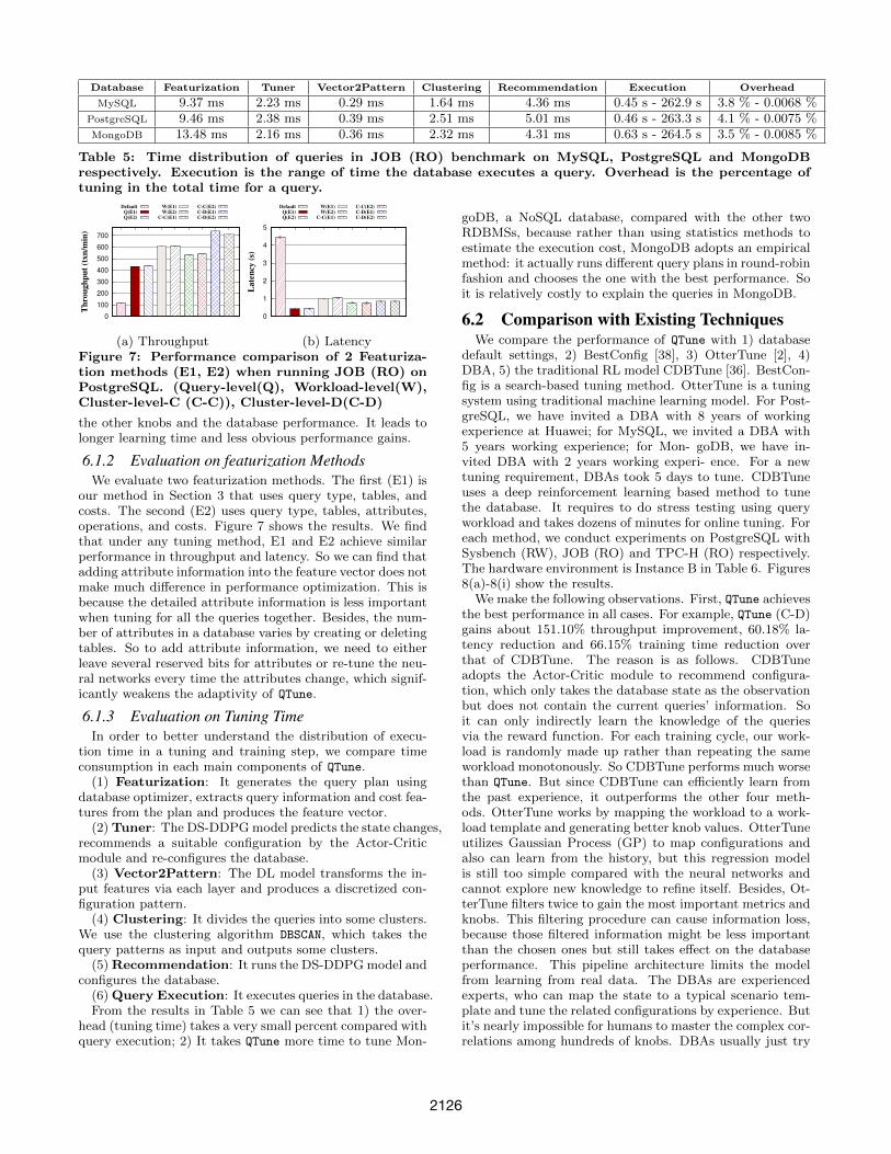
(b) LatencyFigure 7: Performance comparison of 2 Featuriza-tion methods (E1, E2) when running JOB (RO) onPostgreSQL. (Query-level(Q), Workload-level(W),Cluster-level-C (C-C)), Cluster-level-D(C-D)

the other knobs and the database performance. It leads tolonger learning time and less obvious performance gains.

6.1.2 Evaluation on featurization MethodsWe evaluate two featurization methods. The first (E1) is

our method in Section 3 that uses query type, tables, andcosts. The second (E2) uses query type, tables, attributes,operations, and costs. Figure 7 shows the results. We findthat under any tuning method, E1 and E2 achieve similarperformance in throughput and latency. So we can find thatadding attribute information into the feature vector does notmake much difference in performance optimization. This isbecause the detailed attribute information is less importantwhen tuning for all the queries together. Besides, the num-ber of attributes in a database varies by creating or deletingtables. So to add attribute information, we need to eitherleave several reserved bits for attributes or re-tune the neu-ral networks every time the attributes change, which signif-icantly weakens the adaptivity of QTune.

6.1.3 Evaluation on Tuning TimeIn order to better understand the distribution of execu-

tion time in a tuning and training step, we compare timeconsumption in each main components of QTune.

(1) Featurization: It generates the query plan usingdatabase optimizer, extracts query information and cost fea-tures from the plan and produces the feature vector.

(2) Tuner: The DS-DDPG model predicts the state changes,recommends a suitable configuration by the Actor-Criticmodule and re-configures the database.

(3) Vector2Pattern: The DL model transforms the in-put features via each layer and produces a discretized con-figuration pattern.

(4) Clustering: It divides the queries into some clusters.We use the clustering algorithm DBSCAN, which takes thequery patterns as input and outputs some clusters.

(5) Recommendation: It runs the DS-DDPG model andconfigures the database.

(6) Query Execution: It executes queries in the database.From the results in Table 5 we can see that 1) the over-

head (tuning time) takes a very small percent compared withquery execution; 2) It takes QTune more time to tune Mon-

goDB, a NoSQL database, compared with the other twoRDBMSs, because rather than using statistics methods toestimate the execution cost, MongoDB adopts an empiricalmethod: it actually runs different query plans in round-robinfashion and chooses the one with the best performance. Soit is relatively costly to explain the queries in MongoDB.

6.2 Comparison with Existing TechniquesWe compare the performance of QTune with 1) database

default settings, 2) BestConfig [38], 3) OtterTune [2], 4)DBA, 5) the traditional RL model CDBTune [36]. BestCon-fig is a search-based tuning method. OtterTune is a tuningsystem using traditional machine learning model. For Post-greSQL, we have invited a DBA with 8 years of workingexperience at Huawei; for MySQL, we invited a DBA with5 years working experience; for Mon- goDB, we have in-vited DBA with 2 years working experi- ence. For a newtuning requirement, DBAs took 5 days to tune. CDBTuneuses a deep reinforcement learning based method to tunethe database. It requires to do stress testing using queryworkload and takes dozens of minutes for online tuning. Foreach method, we conduct experiments on PostgreSQL withSysbench (RW), JOB (RO) and TPC-H (RO) respectively.The hardware environment is Instance B in Table 6. Figures8(a)-8(i) show the results.

We make the following observations. First, QTune achievesthe best performance in all cases. For example, QTune (C-D)gains about 151.10% throughput improvement, 60.18% la-tency reduction and 66.15% training time reduction overthat of CDBTune. The reason is as follows. CDBTuneadopts the Actor-Critic module to recommend configura-tion, which only takes the database state as the observationbut does not contain the current queries’ information. Soit can only indirectly learn the knowledge of the queriesvia the reward function. For each training cycle, our work-load is randomly made up rather than repeating the sameworkload monotonously. So CDBTune performs much worsethan QTune. But since CDBTune can efficiently learn fromthe past experience, it outperforms the other four meth-ods. OtterTune works by mapping the workload to a work-load template and generating better knob values. OtterTuneutilizes Gaussian Process (GP) to map configurations andalso can learn from the history, but this regression modelis still too simple compared with the neural networks andcannot explore new knowledge to refine itself. Besides, Ot-terTune filters twice to gain the most important metrics andknobs. This filtering procedure can cause information loss,because those filtered information might be less importantthan the chosen ones but still takes effect on the databaseperformance. This pipeline architecture limits the modelfrom learning from real data. The DBAs are experiencedexperts, who can map the state to a typical scenario tem-plate and tune the related configurations by experience. Butit’s nearly impossible for humans to master the complex cor-relations among hundreds of knobs. DBAs usually just try

2126

0

1000

2000

3000

4000

5000

6000

7000

8000

9000T

hro

ug

hp

ut

(tx

n/s

ec)

DefaultBestConfigOtterTune

CDBTuneDBA

QTune(Q)

QTune(W)

(a) Sysbench (RW)

0

100

200

300

400

500

600

700

Th

rou

gh

pu

t (t

xn

/min

)

DefaultBestConfigOtterTune

CDBTuneDBA

QTune(Q)

QTune(W)QTune(C-C)QTune(C-D)

(b) JOB (RO)

0

10

20

30

40

50

Th

rou

gh

pu

t (t

xn

/min

)

DefaultBestConfigOtterTune

CDBTuneDBA

QTune(Q)

QTune(W)QTune(C-C)QTune(C-D)

(c) TPC-H (RO)

0

500

1000

1500

2000

2500

3000

3500

4000

La

ten

cy (

us)

DefaultBestConfigOtterTune

CDBTuneDBA

QTune(Q)

QTune(W)

(d) Sysbench (RW)

0

5

10

15

20

La

ten

cy (

s)

DefaultBestConfigOtterTune

CDBTuneDBA

QTune(Q)

QTune(W)QTune(C-C)QTune(C-D)

(e) JOB (RO)

0

100

200

300

400

500

600

700

800

La

ten

cy (

s)

DefaultBestConfigOtterTune

CDBTuneDBA

QTune(Q)

QTune(W)QTune(C-C)QTune(C-D)

(f) TPC-H (RO)

0

10

20

30

40

50

60

70

Tra

inin

gT

ime

(h)

BestConfigOtterTune

CDBTuneQTune(Q)

QTune(W)

(g) Sysbench (RW)

0

10

20

30

40

50

60

70

Tra

inin

gT

ime

(h)

BestConfigOtterTuneCDBTune

QTune(Q)QTune(W)

QTune(C-C)

QTune(C-D)

(h) JOB (RO)

0

10

20

30

40

50

60

70

Tra

inin

gT

ime

(h)

BestConfigOtterTuneCDBTune

QTune(Q)QTune(W)

QTune(C-C)

QTune(C-D)

(i) TPC-H (RO)Figure 8: Comparison with existing methods Default settings, BestConfig, OtterTune, CDBTune, DBA onSysbench (RW), JOB (RO) and TPC-H (RO) on PostgreSQL. QTune (Q) represents query-level tunig. QTune

(W) represents workload-level tuning. And QTune (C-C) and QTune (C-D) indicate cluster-level tuning usingContinuous Tuner and Discrete Tuner respectively.

several impactful knobs. With rich experience they can finda usable configuration in a short time, but the results areusually not good enough. Moreover, it takes DBAs verylong time to figure out an ideal knob pattern. BestConfigstarts by randomly choosing some knob combinations andexplores from the best configuration points iteratively. Sincethe provided resource is limited, it usually can only gain asub-optimal configuration. Besides, each searching periodrestarts and cannot utilize the past searching results. Sothe performance improvement is not very good sometimes.

Second, QTune (C-D), cluster-level tuning with discretetuner, achieves the highest throughput, because it makesgood tradeoff between providing good knobs for a group ofqueries and achieving high tuning time. QTune (Q), query-level tuning achieves the lowest latency, because it providesthe best knob values for each query.

Third, CDBTune takes the longest training time. On theone hand, in each training cycle, it requires to run trainingexamples on the databases, which is time consuming. Onthe other hand, it only tunes according to the database stateand without filtering it utilizes all the dynamic knobs, whichtakes longer time to meet the performance requirements. In-

stead, the training time of BestConfig is controlled by theresource limits. OtterTune recommends configurations ac-cording to both the workload and performance metrics anddo not need to actually run the training examples.

Fourth, our method has much larger improvement on TPC-H than JOB and Sysbench. This is because TPC-H simu-lates the real OLAP working scenarios and each query con-tains many complex operations, such as the “join”. In orderto support such complex workload, QTune has large improve-ment space to explore and thus gets great gains by efficientlyanalyzing the query characters and database states. Andqueries in JOB also contain many join operations and arecostly to execute, and thus QTune still can optimize the queryplan and execution procedure. But in Sysbench, the queriesare simple and randomly produced based on several simplerules. They have similar structures and take few resourcesto finish. So the improvement is not obvious in Sysbench.Considering the other methods, we find the performance ofthe traditional RL model is still not bad, only worse thanQTune on the three benchmarks. It can verify that it isfeasible to use reinforcement learning in database tuning.And the performance of DBA and OtterTune is not steady.

2127

0

1000

2000

3000

4000

5000

6000

7000

8000

9000

Th

rou

gh

pu

t (t

xn

/sec

)Default

BestConfigOtterTune

CDBTuneDBA

QTune(Q)

QTune(W)

(a) JOB(RO) to Sysb.(RW)

0

500

1000

1500

2000

2500

3000

3500

4000

La

ten

cy (

us)

DefaultBestConfigOtterTune

CDBTuneDBA

QTune(Q)

QTune(W)

(b) JOB(RO) to Sysb.(RW)

0

100

200

300

400

500

600

700

Th

rou

gh

pu

t (t

xn

/min

)

DefaultBestConfigOtterTune

CDBTuneDBA

QTune(Q)

QTune(W)QTune(C-C)QTune(C-D)

(c) TPC-H(RO) to JOB(RO)

0

5

10

15

20

La

ten

cy (

s)

DefaultBestConfigOtterTune

CDBTuneDBA

QTune(Q)

QTune(W)QTune(C-C)QTune(C-D)

(d) TPC-H(RO) to JOB(RO)Figure 9: Performance when workload changes on PostgreSQL.

Because it is a bit tough for humans and the shallow ma-chine learning methods to handle the tuning problem withdifferent workload and data sets. For the throughput, theresults are similar. And we can find from the training timethat QTune is quite efficient to learn knowledge from a com-pletely new starting point. But it takes relatively long timefor DBA, OtterTune and the traditional RL to converge.

In summary, the DS-DDPG model suits this tuning sce-nario better. Rather than blindly tuning without the knowl-edge of the tasks to be conducted, QTune characterizes thequeries and integrates these query features and databasestate into the DRL model. QTune can provide much bet-ter decision based on these two aspects. Besides, for work-loads like OLAP, we can divide them into different clusters(cluster-level) and execute the queries by cluster.

6.3 Evaluation on Generalization6.3.1 Varying Different Workloads

We verify the performance of QTune when workload changes.On PostgreSQL, we conduct two experiments: 1) Use themodel trained on JOB (RO) benchmark to tune databaseon Sysbench (RW) benchmark; 2) Use the model trainedon TPC-H (RO) benchmark to tune database on JOB (RO)benchmark. And we compare QTune with database defaultsettings, BestConfig, OtterTune, CDBTune and DBA. Fig-ures 9(a) to 9(d) show the results. Note that JOB queriesvary in time and resource consumption, but there are only113 queries. So we expend JOB into 10000 queries, based onthe data set and existing query structures. We also extendTPC-H benchmark to generate more queries.

First, we apply these trained model for JOB (RO) to Sys-bench (RW) and evaluate the performance. We make thefollowing observations. First, QTune still outperforms thebaselines. Query-level or workload-level tuning can adaptto query changes from Sysbench (RW). Since the optimalknob space changes after altering workload, it’s tough forBestConfig to recommend suitable configurations withoutenough time to search. Since OtterTune relies on workloadto map configuration patterns, it actually suffers most fromthe change. While CDBTune is free from these problemsand even preforms better for JOB. This is because CDB-Tune does not consider queries directly and only observesthe changes in database state. QTune performs better, be-cause queries are vectorized by Query2Vector and utilizedby Predictor. The query features include the data distribu-tion and query costs. So our model is capable of adapting todifferent workloads. And even if the table schemas are differ-ent across different benchmarks, the difference in data scaleand cost features can be obtained and the tuning model canrecommend different configuration based on such difference.

Second, for TPC-H (RO) to JOB (RO), the results aresimilar. For JOB (RO), first, QTune performs the best amongthe five tuning methods. In general, TPC-H queries are

Table 6: Two hardware configurations

Instance RAM (GB) Disk (GB) CPU (GHz)

A 16 780 2.49B 128 5000 4.00

much more complex than JOB queries, and QTune can eas-ily utilize the knowledge learned from the query featuresof TPC-H to correctly estimate new feature vectors parsedfrom JOB, so QTune outperforms the others even if the work-load changes. Moreover, compared with Figures 9(a)-9(b),the performance of QTune changes little. While the perfor-mance of BestConfig and OtterTune gets worse because it’stough for them to adapt to new workloads in a short time.The performance of CDBTune turns better because it’s ca-pable of adjusting the model according to the state change.

6.3.2 Varying Different DatabasesDifferent databases have completely different system pa-

rameters, including different meanings, types, names andvalue ranges. Besides, RDBMSs may have very similar op-erating mechanisms, but NoSQL databases are completelydifferent, e.g., MongoDB is based on key-value data struc-tures and lacks of many concepts in RDBMSs such as for-eign keys. To verify that QTune can perform well on dif-ferent databases, we use three other databases to conductexperiments. We run JOB on MySQL and run TPC-H onMongoDB. For each experiment, the performance of QTune

is compared with the other four methods. Figures 10(a)-10(d) show the results. We have the following observations.

First, QTune performs well on the three databases andoutperforms the other four methods. This is contributed toour query-aware tuning techniques. Second, on MongoDB,QTune achieves the best performance improvement. This isbecause operating mechanisms such as index optimizationsand task scheduling are not as good as RDBMS like MySQL,and PostgreSQL and MongoDB is more sensitive to differentdatabase configurations. Third, latency reduction is muchless than throughput improvement, because we have largeopportunity to tune throughput but less opportunity to tunelatency. Fourth, QTune can efficiently adapt to different en-vironments and keep in relatively good performance.

6.3.3 Varying Different Hardware environmentsIt is a challenge to adapt to new hardware environment,

because the learnt knowledge of the disk size, RAM size andcomputing ability needs to be updated when the model ismigrated to a different hardware environments. We conductexperiment to evaluate whether QTune can adapt to newhardware environments. We use two instances as shown inTable 6. B is better than A in each aspect. So the modeltrained on A has very large configuration space to exploreonce it’s migrated to B. As shown in Figures 11(a)-11(d),M B on A (model trained on B is used to tune on A) per-forms even better than M A on A (model trained on A isused to tune on A). This is because the model trained on B

2128

0

200

400

600

800

1000

Th

rou

gh

pu

t (t

xn

/min

)Default

BestConfigOtterTune

CDBTuneDBA

QTune(Q)

QTune(W)QTune(C-C)QTune(C-D)

(a) MySQL

0

5

10

15

20

La

ten

cy (

s)

DefaultBestConfigOtterTune

CDBTuneDBA

QTune(Q)

QTune(W)QTune(C-C)QTune(C-D)

(b) MySQL

0

10

20

30

40

50

Th

rou

gh

pu

t (t

xn

/min

)

DefaultBestConfigOtterTune

CDBTuneDBA

QTune(Q)

QTune(W)QTune(C-C)QTune(C-D)

(c) MongoDB

0

100

200

300

400

500

600

700

800

La

ten

cy (

s)

DefaultBestConfigOtterTune

CDBTuneDBA

QTune(Q)

QTune(W)QTune(C-C)QTune(C-D)

(d) MongoDBFigure 10: Performance for different databases.

0

100

200

300

400

500

600

Th

rou

gh

pu

t (t

xn

/min

)

DefaultBestConfigOtterTune

CDBTuneDBA

QTune(Q)

QTune(W)QTune(C-C)QTune(C-D)

(a) M A on A

0

5

10

15

20

25

La

ten

cy (

s)

DefaultBestConfigOtterTune

CDBTuneDBA

QTune(Q)

QTune(W)QTune(C-C)QTune(C-D)

(b) M A on A

0

200

400

600

800

1000

1200

Th

rou

gh

pu

t (t

xn

/min

)

DefaultBestConfigOtterTune

CDBTuneDBA

QTune(Q)

QTune(W)QTune(C-C)QTune(C-D)

(c) M B on A

0

5

10

15

20

25

La

ten

cy (

s)

DefaultBestConfigOtterTune

CDBTuneDBA

QTune(Q)

QTune(W)QTune(C-C)QTune(C-D)

(d) M B on AFigure 11: Performance for different hardware environments.

has already explored large enough configuration space whichoverlaps the optimal information of instance A, or includesbetter configuration space than that by M A. And for eachknob value recommended by model B, if it’s above the al-lowed range, we will change it to the boundary value. Sothere can be many “invalid” recommendations, but this usu-ally won’t cause resource waste. And this convergence isfaster than exploring for new optimal space.

7. RELATED WORKDatabase Tuning. There has been several studies on au-tomatic database tuning, which can be divided into two cat-egories: rule-based methods and learning-based methods.(1) Rule-based Methods. Rule-based methods explore op-timal database configurations by using rules or heuristics.iTuned [7] uses statistical methods to find most impact-ful knobs and tune database according to the correlationsof performance and knobs. Wei et al. [33] propose a per-formance tuning framework which generates rules and usesthese rules to conduct tuning. BestConfig [38] divides thehigh-dimension knob space into subspaces and iterativelychooses configurations using recursive bound and search.However they rely on either rules or history data.(2) Learning-based Methods. Learning-based methods uti-lize the machine learning techniques to tune database knobs.OtterTune [2] uses a traditional ML model to map a work-load to a specific configuration. However it relies on large-scale high-quality training samples. Zheng et al. [37] proposeto identify key system parameters using statistical methodsand utilize a neural network to match configurations for aspecific workload. It also requires large volume of trainingsamples and has the problem of overfitting. CDBTune [36]utilizes a DRL model that recommends configurations basedon the database states. However, it only provides a coarse-grained tuning but cannot provide fine-grained tuning.Reinforcement Learning. Reinforcement learning (RL)was proposed to address game theory [24, 9, 23]. RL isa framework that enables a learner (agent) to take actionsin a specific scenario (environment) and learn from the in-teractions with the environment in discrete time steps [24].Unlike supervised learning, RL does not need a large volumeof training data. Instead, through trial and error, the agent

iteratively optimizes its policy of choosing actions, with thegoal of maximizing an objective function (reward). By theexploration and exploitation mechanism, RL can make atradeoff between exploring untouched space and exploitingcurrent knowledge. But the traditional RL approaches havedifficulty in choosing the state features [22]. Mnih et al. [21]propose a DRL model combining RL with deep learningmethods to solve problems with limited prior knowledge andhigh-dimensional state space. And many DRL algorithms,such as DQN [30] and DDPG [16], have been successfullyutilized in different optimal problems [17, 3, 35, 15, 31].

There have been many researches in solving database prob-lems with reinforcement learning [13]. Basu et al. proposedto learn the cost model with RL and use this learnt knowl-edge to implement index tuning [4]. Tzoumas et al. [29]assume a suitable query plan residing in the routing policiesand they use a RL model to learn the policies. ReJoin [20]optimizes query plans by enumerating join orderings withRL. Sun et al. [28] proposed an end-to-end cost estimator.SageDB [11] provides a vision that the core components ina database may be replaced by learned models. Li et al. [14]propose AI-native databases that not only utilize AI to op-timize databases but provide in-database AI capabilities.

8. CONCLUSIONWe proposed a query-aware database tuning system QTune

with a deep reinforcement learning (DRL) model. QTune fea-turized the SQL queries by considering rich features of theSQL queries. QTune fed the query vectors into the DRLmodel to dynamically choose suitable configurations. OurDRL model used the the actor-critic networks to find opti-mal configurations according to both the current and pre-dicted database states. Our tuning system can supportquery-level, workload-level and cluster-level database tun-ing. We also proposed a query clustering method using deeplearning model to enable cluster-level tuning. Experimentalresults showed that QTune achieved high performance andoutperformed the state-of-the-art tuning methods.Acknowledgement This work was supported by the 973Program of China (2015CB358700), NSF of China (61632016,61521002, 61661166012), Huawei, and TAL education. Guo-liang Li is the corresponding author.

2129

9. REFERENCES[1] A. F. Agarap. Deep learning using rectified linear

units (relu). CoRR, abs/1803.08375, 2018.

[2] D. V. Aken, A. Pavlo, G. J. Gordon, and B. Zhang.Automatic database management system tuningthrough large-scale machine learning. In SIGMOD,pages 1009–1024, 2017.

[3] R. Ali, N. Shahin, Y. B. Zikria, B. Kim, and S. W.Kim. Deep reinforcement learning paradigm forperformance optimization of channelobservation-based MAC protocols in dense wlans.IEEE Access, 7:3500–3511, 2019.

[4] D. Basu, Q. Lin, W. Chen, H. T. Vo, Z. Yuan,P. Senellart, and S. Bressan. Regularized cost-modeloblivious database tuning with reinforcement learning.T. Large-Scale Data- and Knowledge-CenteredSystems, 28:96–132, 2016.

[5] P. Belknap, B. Dageville, K. Dias, and K. Yagoub.Self-tuning for SQL performance in oracle database11g. In ICDE, pages 1694–1700, 2009.

[6] S. G. Dikaleh, D. Xiao, C. Felix, D. Mistry, andM. Andrea. Introduction to neural networks. InCASCON, page 299, 2017.

[7] S. Duan, V. Thummala, and S. Babu. Tuningdatabase configuration parameters with ituned.PVLDB, 2(1):1246–1257, 2009.

[8] M. Ester, H. Kriegel, J. Sander, and X. Xu. Adensity-based algorithm for discovering clusters inlarge spatial databases with noise. In KDD, pages226–231, 1996.

[9] V. Francois-Lavet, P. Henderson, R. Islam, M. G.Bellemare, and J. Pineau. An introduction to deepreinforcement learning. CoRR, abs/1811.12560, 2018.

[10] D. P. Kingma and J. Ba. Adam: A method forstochastic optimization. CoRR, abs/1412.6980, 2014.

[11] T. Kraska, M. Alizadeh, A. Beutel, E. H. Chi,A. Kristo, G. Leclerc, S. Madden, H. Mao, andV. Nathan. Sagedb: A learned database system. InCIDR, 2019.

[12] S. Krishnan. Hierarchical Deep ReinforcementLearning For Robotics and Data Science. PhD thesis,University of California, Berkeley, USA, 2018.

[13] G. Li. Human-in-the-loop data integration. PVLDB,10(12):2006–2017, 2017.

[14] G. Li, X. Zhou, and S. Li.Xuanyuan:anai-nativedatabase. In IEEE DataBulletin, 2019.

[15] K. Li and G. Li. Approximate query processing: Whatis new and where to go? Data Science andEngineering, 3(4):379–397, 2018.

[16] T. P. Lillicrap, J. J. Hunt, A. Pritzel, N. Heess,T. Erez, Y. Tassa, D. Silver, and D. Wierstra.Continuous control with deep reinforcement learning.CoRR, abs/1509.02971, 2015.

[17] R. Lin, M. D. Stanley, M. M. Ghassemi, andS. Nemati. A deep deterministic policy gradientapproach to medication dosing and surveillance in theICU. In EMBC, pages 4927–4931, 2018.

[18] O. Luaces, J. Dıez, J. Barranquero, J. J. del Coz, andA. Bahamonde. Binary relevance efficacy for

multilabel classification. Progress in AI, 1(4):303–313,2012.

[19] V. Maglogiannis, D. Naudts, A. Shahid, andI. Moerman. A q-learning scheme for fair coexistencebetween LTE and wi-fi in unlicensed spectrum. IEEEAccess, 6:27278–27293, 2018.

[20] R. Marcus and O. Papaemmanouil. Deepreinforcement learning for join order enumeration. InSIGMOD workshop, pages 3:1–3:4, 2018.

[21] V. Mnih, K. Kavukcuoglu, D. Silver, and etc.Human-level control through deep reinforcementlearning. Nature, 518(7540):529–533, 2015.

[22] R. Munos and A. W. Moore. Variable resolutiondiscretization in optimal control. Machine Learning,49(2-3):291–323, 2002.

[23] Z. Ni, H. He, D. Zhao, and D. V. Prokhorov.Reinforcement learning control based on multi-goalrepresentation using hierarchical heuristic dynamicprogramming. In IJCNN, pages 1–8, 2012.

[24] A. Nowe and T. Brys. A gentle introduction toreinforcement learning. In SUM, pages 18–32, 2016.

[25] J. S. Oh and S. H. Lee. Resource selection forautonomic database tuning. In ICDE, page 1218, 2005.

[26] J. Read, B. Pfahringer, G. Holmes, and E. Frank.Classifier chains for multi-label classification. MachineLearning, 85(3):333–359, 2011.

[27] D. G. Sullivan, M. I. Seltzer, and A. Pfeffer. Usingprobabilistic reasoning to automate software tuning.In SIGMETRICS, pages 404–405, 2004.

[28] J. Sun and G. Li. An end-to-end learning-based costestimator. CoRR, abs/1906.02560, 2019.

[29] K. Tzoumas, T. Sellis, and C. S. Jensen. Areinforcement learning approach for adaptive queryprocessing. 2008.

[30] H. van Hasselt. Double q-learning. In NIPS, pages2613–2621, 2010.

[31] G. Vargas-Solar, J.-L. Zechinelli-Martini, and J.-A.Espinosa-Oviedo. Big data management: What tokeep from the past to face future challenges? DataScience and Engineering, 2(4):328–345, 2017.

[32] C. Watkins and P. Dayan. Technical note q-learning.Machine Learning, 8:279–292, 1992.

[33] Z. Wei, Z. Ding, and J. Hu. Self-tuning performance ofdatabase systems based on fuzzy rules. In FSKD,pages 194–198, 2014.

[34] G. Weikum, A. Monkeberg, C. Hasse, and P. Zabback.Self-tuning database technology and informationservices: from wishful thinking to viable engineering.In VLDB, pages 20–31, 2002.

[35] E. Wu. Crazy idea! databases reinforcement-learningresearch. In CIDR, 2019.

[36] J. Zhang, Y. Liu, K. Zhou, and G. Li. An end-to-endautomatic cloud database tuning system using deepreinforcement learning. In SIGMOD, 2019.

[37] C. Zheng, Z. Ding, and J. Hu. Self-tuning performanceof database systems with neural network. In ICIC,pages 1–12, 2014.

[38] Y. Zhu, J. Liu, M. Guo, Y. Bao, W. Ma, Z. Liu,K. Song, and Y. Yang. Bestconfig: tapping theperformance potential of systems via automaticconfiguration tuning. In SoCC, pages 338–350, 2017.

2130