
QSupQuestions6
59
Quantitative Analysis BA 452 Supplemental Questions 6 1 This document contains practice questions that supplement homework questions and review questions for Lessons II-1 and II-2. This document first identifies the learning objectives of solving supplemental questions. The document then lists 36 questions. Four of those questions (questions 7, 11, 15, and 19) are like the questions in Homework 6. Finally, the document answers all questions except the homework questions. All questions can be helpful except questions 29 to 36. Questions marked with an asterisk * are similar to review questions. Tip: Supplemental questions are grouped into sets of similar type. Once you have mastered the questions in a set, you can skip the rest of the questions in that set.
-
Upload
byeongsoo-yoo -
Category
Documents
-
view
2.016 -
download
89
Transcript of QSupQuestions6

Quantitative Analysis BA 452 Supplemental Questions 6
1
This document contains practice questions that supplement homework questions and review questions for Lessons II-1 and II-2. This document first identifies the learning objectives of solving supplemental questions. The document then lists 36 questions. Four of those questions (questions 7, 11, 15, and 19) are like the questions in Homework 6. Finally, the document answers all questions except the homework questions. All questions can be helpful except questions 29 to 36. Questions marked with an asterisk * are similar to review questions.
Tip: Supplemental questions are grouped into sets of similar type. Once you have mastered the questions in a set, you can skip the rest of the questions in that set.

Quantitative Analysis BA 452 Supplemental Questions 6
2
Objectives By working through the homework questions and the supplemental questions, you will:
1. Be able to identify the special features of the transportation
problem. 2. Become familiar with the types of problems that can be solved by
applying a transportation model. 3. Be able to develop network and linear programming models of
the transportation problem. 4. Know how to handle the cases of (1) unequal supply and
demand, (2) unacceptable routes, and (3) maximization objective for a transportation problem.
5. Be able to identify the special features of the assignment
problem. 6. Become familiar with the types of problems that can be solved by
applying an assignment model. 7. Be able to develop network and linear programming models of
the assignment problem. 8. Be familiar with the special features of the transshipment
problem. 9. Become familiar with the types of problems that can be solved by
applying a transshipment model. 10 Be able to develop network and linear programming models of
the transshipment problem. 11. Know the basic characteristics of the shortest route problem. 12. Be able to develop a linear programming model and solve the
shortest route problem.

Quantitative Analysis BA 452 Supplemental Questions 6
3
13. Know the basic characteristics of the maximal flow problem. 14. Be able to develop a linear programming model and solve the
maximal flow problem. 15. Know how to structure and solve a production and inventory
problem as a transshipment problem.
16. Understand the following terms:
network flow problem shortest route transportation problem source node origin sink node destination assignment problem transshipment problem

Quantitative Analysis BA 452 Supplemental Questions 6
4
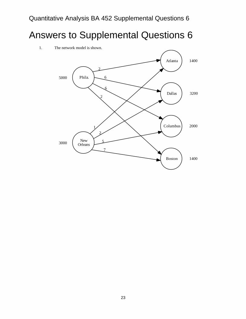
Supplemental Questions 6 1. A company imports goods at two ports: Philadelphia and New Orleans. Shipments of one product
are made to customers in Atlanta, Dallas, Columbus, and Boston. For the next planning period, the supplies at each port, customer demands, and shipping costs per case from each port to each customer are as follows:
Customers Port Atlanta Dallas Columbus Boston Port Supply Philadelphia 2 6 6 2 5000 New Orleans 1 2 5 7 3000
Demand 1400 3200 2000 1400 Develop a network representation of the distribution system (transportation problem).
2. Consider the following network representation of a transportation problem:
The supplies, demands, and transportation costs per unit are shown on the network. a. Develop a linear programming model for this problem; be sure to define the variables in your
model. b. Solve the linear program to determine the optimal solution.
Quantitative Analysis BA 452 Supplemental Questions 6
5
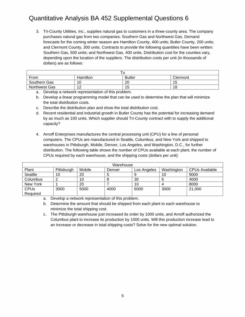
3. Tri-County Utilities, Inc., supplies natural gas to customers in a three-county area. The company purchases natural gas from two companies: Southern Gas and Northwest Gas. Demand forecasts for the coming winter season are Hamilton County, 400 units; Butler County, 200 units; and Clermont County, 300 units. Contracts to provide the following quantities have been written: Southern Gas, 500 units; and Northwest Gas, 400 units. Distribution cost for the counties vary, depending upon the location of the suppliers. The distribution costs per unit (in thousands of dollars) are as follows:
To From Hamilton Butler Clermont Southern Gas 10 20 15 Northwest Gas 12 15 18
a. Develop a network representation of this problem. b. Develop a linear programming model that can be used to determine the plan that will minimize
the total distribution costs. c. Describe the distribution plan and show the total distribution cost. d. Recent residential and industrial growth in Butler County has the potential for increasing demand
by as much as 100 units. Which supplier should Tri-County contract with to supply the additional capacity?
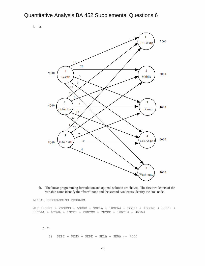
4. Arnoff Enterprises manufactures the central processing unit (CPU) for a line of personal computers. The CPUs are manufactured in Seattle, Columbus, and New York and shipped to warehouses in Pittsburgh, Mobile, Denver, Los Angeles, and Washington, D.C., for further distribution. The following table shows the number of CPUs available at each plant, the number of CPUs required by each warehouse, and the shipping costs (dollars per unit):
Warehouse Plant Pittsburgh Mobile Denver Los Angeles Washington CPUs Available Seattle 10 20 5 9 10 9000 Columbus 2 10 8 30 6 4000 New York 1 20 7 10 4 8000 CPUs Required
3000 5000 4000 6000 3000 21,000
a. Develop a network representation of this problem. b. Determine the amount that should be shipped from each plant to each warehouse to
minimize the total shipping cost. c. The Pittsburgh warehouse just increased its order by 1000 units, and Arnoff authorized the
Columbus plant to increase its production by 1000 units. Will this production increase lead to an increase or decrease in total shipping costs? Solve for the new optimal solution.

Quantitative Analysis BA 452 Supplemental Questions 6
6
5. Premier Consulting’s two consultants, Avery and Baker, can be scheduled to work for clients up to a maximum of 160 hours each over the next four weeks. A third consultant, Campbell, has some administrative assignments already planned and is available for clients up to a maximum of 140 hours over the next four weeks. The company has four clients with projects in process. The estimated hourly requirements for each of the clients over the four-week period are
Client Hours A 180 B 75 C 100 D 85
Hourly rates vary for the consultant-client combination and are based on several factors, including project type and the consultant’s experience. The rates (dollars per hour) for each consultant-client combination are as follows:
Client Consultant A B C D Avery 100 125 115 100 Baker 120 135 115 120 Campbell 155 150 140 130
a. Develop a network representation of the problem. b. Formulate the problem as a linear program, with the optimal solution providing the hours
each consultant should be scheduled for each client to maximize the consulting firm’s billings. What is the schedule and what is the total billing?
c. New information shows that Avery doesn’t have the experience to be scheduled for client B. If this consulting assignment is not permitted, what impact does it have on total billings? What is the revised schedule?
6. Klein Chemicals, Inc., produces a special oil-based material that is currently in short supply. Four
of Klein’s customers have already placed orders that together exceed the combined capacity of Klein’s two plants. Klein’s management faces the problem of deciding how many units it should supply to each customer. Because the four customers are in different industries, different prices can be charged because of the various industry pricing structures. However, slightly different production costs at the two plants and varying transportation cost between the plants and customers make a “sell to the highest bidder” strategy unacceptable. After considering price, production costs, and transportation costs, Klein established the following profit per unit for each plant-customer alternative:
Customer Plant D-1 D-2 D-3 D-4 Clifton Springs $32 $34 $32 $40 Danville $34 $30 $28 $38 The plant capacities and customer orders are as follows: Plant Capacity (units) Distributor Orders (units) Clifton Springs 5000 D1: 2000
D2: 5000 Danville 3000 D3: 3000
D4: 2000
How many units should each plant produce for each customer in order to maximize profits? Which customer demands will not be met? Show your network model and linear programming formulation.
Quantitative Analysis BA 452 Supplemental Questions 6
7
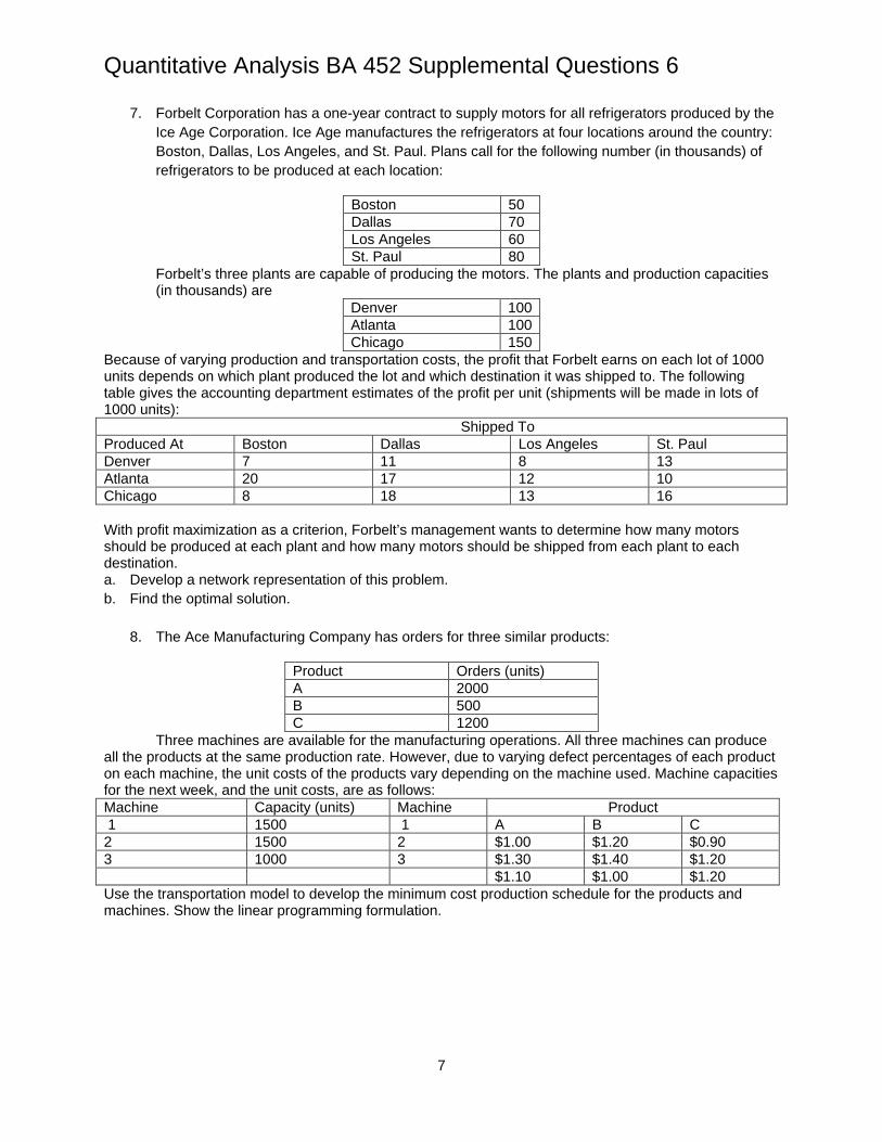
7. Forbelt Corporation has a one-year contract to supply motors for all refrigerators produced by the Ice Age Corporation. Ice Age manufactures the refrigerators at four locations around the country: Boston, Dallas, Los Angeles, and St. Paul. Plans call for the following number (in thousands) of refrigerators to be produced at each location:
Boston 50 Dallas 70 Los Angeles 60 St. Paul 80
Forbelt’s three plants are capable of producing the motors. The plants and production capacities (in thousands) are
Denver 100 Atlanta 100 Chicago 150
Because of varying production and transportation costs, the profit that Forbelt earns on each lot of 1000 units depends on which plant produced the lot and which destination it was shipped to. The following table gives the accounting department estimates of the profit per unit (shipments will be made in lots of 1000 units): Shipped To Produced At Boston Dallas Los Angeles St. Paul Denver 7 11 8 13 Atlanta 20 17 12 10 Chicago 8 18 13 16 With profit maximization as a criterion, Forbelt’s management wants to determine how many motors should be produced at each plant and how many motors should be shipped from each plant to each destination. a. Develop a network representation of this problem. b. Find the optimal solution.
8. The Ace Manufacturing Company has orders for three similar products:
Product Orders (units) A 2000 B 500 C 1200
Three machines are available for the manufacturing operations. All three machines can produce all the products at the same production rate. However, due to varying defect percentages of each product on each machine, the unit costs of the products vary depending on the machine used. Machine capacities for the next week, and the unit costs, are as follows: Machine Capacity (units) Machine Product 1 1500 1 A B C 2 1500 2 $1.00 $1.20 $0.90 3 1000 3 $1.30 $1.40 $1.20 $1.10 $1.00 $1.20 Use the transportation model to develop the minimum cost production schedule for the products and machines. Show the linear programming formulation.
Quantitative Analysis BA 452 Supplemental Questions 6
8
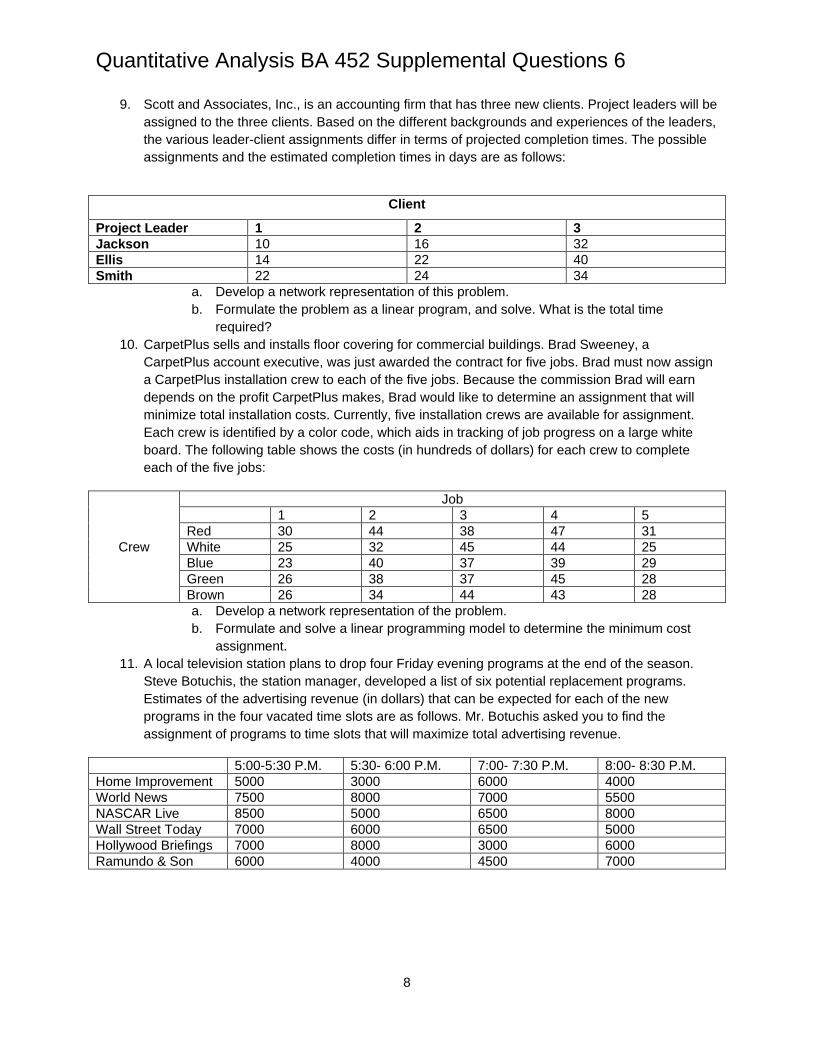
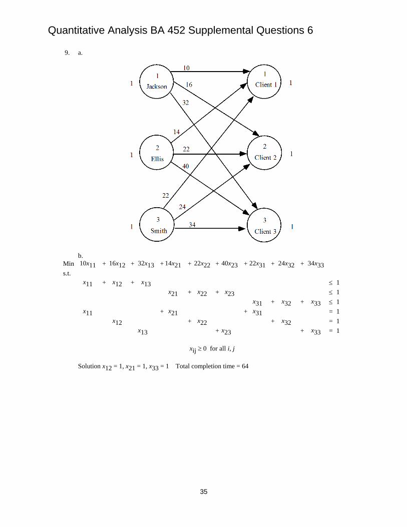
9. Scott and Associates, Inc., is an accounting firm that has three new clients. Project leaders will be assigned to the three clients. Based on the different backgrounds and experiences of the leaders, the various leader-client assignments differ in terms of projected completion times. The possible assignments and the estimated completion times in days are as follows:
Client
Project Leader 1 2 3 Jackson 10 16 32 Ellis 14 22 40 Smith 22 24 34
a. Develop a network representation of this problem. b. Formulate the problem as a linear program, and solve. What is the total time
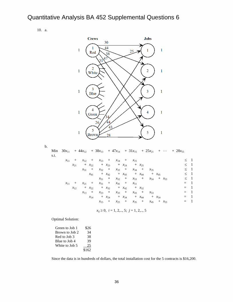
required? 10. CarpetPlus sells and installs floor covering for commercial buildings. Brad Sweeney, a
CarpetPlus account executive, was just awarded the contract for five jobs. Brad must now assign a CarpetPlus installation crew to each of the five jobs. Because the commission Brad will earn depends on the profit CarpetPlus makes, Brad would like to determine an assignment that will minimize total installation costs. Currently, five installation crews are available for assignment. Each crew is identified by a color code, which aids in tracking of job progress on a large white board. The following table shows the costs (in hundreds of dollars) for each crew to complete each of the five jobs:
Crew
Job 1 2 3 4 5 Red 30 44 38 47 31 White 25 32 45 44 25 Blue 23 40 37 39 29 Green 26 38 37 45 28 Brown 26 34 44 43 28 a. Develop a network representation of the problem. b. Formulate and solve a linear programming model to determine the minimum cost
assignment. 11. A local television station plans to drop four Friday evening programs at the end of the season.
Steve Botuchis, the station manager, developed a list of six potential replacement programs. Estimates of the advertising revenue (in dollars) that can be expected for each of the new programs in the four vacated time slots are as follows. Mr. Botuchis asked you to find the assignment of programs to time slots that will maximize total advertising revenue.
5:00-5:30 P.M. 5:30- 6:00 P.M. 7:00- 7:30 P.M. 8:00- 8:30 P.M. Home Improvement 5000 3000 6000 4000 World News 7500 8000 7000 5500 NASCAR Live 8500 5000 6500 8000 Wall Street Today 7000 6000 6500 5000 Hollywood Briefings 7000 8000 3000 6000 Ramundo & Son 6000 4000 4500 7000

Quantitative Analysis BA 452 Supplemental Questions 6
9
12. The U.S. Cable Company uses a distribution system with five distribution centers and eight customer zones. Each customer zone is assigned a sole source supplier; each customer zone receives all of its cable products from the same distribution center. In an effort to balance demand and workload at the distribution centers, the company’s vice president of logistics specified that distribution centers may not be assigned more than three customer zones. The following table shows the five distribution centers and cost of supplying each customer zone (in thousands of dollars):
Customer Zones Distribution Centers
Los Angeles
Chicago Columbus Atlanta Newark Kansas City
Denver Dallas
Plano 70 47 22 53 98 21 27 13 Nashville 75 38 19 58 90 34 40 26 Flagstaff 15 78 37 82 111 40 29 32 Springfield 60 23 8 39 82 36 32 45 Boulder 45 40 29 75 86 25 11 37
a. Determine the assignment of customer zones to distribution centers that will minimize cost.
b. Which distribution centers, if any, are not used? c. Suppose that each distribution center is limited to a maximum of two customer zones.
How does this constraint change the assignment and the cost of supplying customer zones?
13. United Express Service (UES) uses large quantities of packaging materials as its four distribution
hubs. After screening potential suppliers, UES identified six vendors that can provide packaging materials that will satisfy its quality standards. UES asked each of the six vendors to submit bids to satisfy annual demand at each of its four distribution hubs over the next year. The following table lists the bids received (in thousands of dollars). UES wants to ensure that each of the distribution hubs is serviced by a different vendor. Which bids should UES accept, and which vendors should UES select to supply each distribution hub?
Distribution Hub Bidder 1 2 3 4 Martine products 190 175 125 230 Schmidt Materials 150 235 155 220 Miller Containers 210 225 135 260 D&J Burns 170 185 190 280 Larbes Furnishings
220 190 140 240
Lawler Depot 270 200 130 260

Quantitative Analysis BA 452 Supplemental Questions 6
10
14. The quantitative methods department head at a major Midwestern university will be scheduling faculty to teach courses during the coming autumn term. Four core courses need to be covered. The four courses are at the UG, MBA, MS, and Ph.D. levels. Four professors will be assigned to the courses, with each professor receiving one of the courses. Student evaluations of professors are available from previous terms. Based on a rating scale of 4 (excellent), 3 (very good), 2 (average), 1 (fair), and 0 (poor), the average student evaluations for each professor are shown. Professor D does not have a Ph.D. and cannot be assigned to teach the Ph.D.-level course. If the department head makes teaching assignments based on maximizing the student evaluation ratings over all four courses, what staffing assignments should be made?
Course Professor UG MBA MS Ph.D. A 2.8 2.2 3.3 3.0 B 3.2 3.0 3.6 3.6 C 3.3 3.2 3.5 3.5 D 3.2 2.8 2.5 -
15. A market research film’s three clients each requested that the firm conduct a sample survey. Four
available statisticians can be assigned to these three projects; however, all four statisticians are busy, and therefore each can handle only one client. The following data show the number of hours required for each statistician to complete each job; the differences in time are based on experience and ability of the statisticians.
Client Statistician A B C 1 150 210 270 2 170 230 220 3 180 230 225 4 160 240 230
a. Formulate and solve a linear programming model for this problem. b. Suppose that the time statistician 4 needs to complete the job for client A is
increased from 160 to 165 hours. What effect will this change have on the solution? c. Suppose that the time statistician 4 needs to complete the job for client A is
decreased to 140 hours. What effect will this change have on the solution? d. Suppose that the time statistician 3 needs to complete the job for client B increases
to 250 hours. What effect will this change have on the solution?
Quantitative Analysis BA 452 Supplemental Questions 6
11
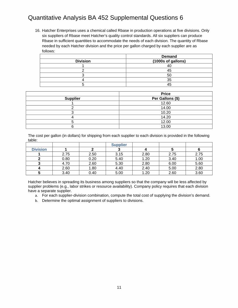
16. Hatcher Enterprises uses a chemical called Rbase in production operations at five divisions. Only six suppliers of Rbase meet Hatcher’s quality control standards. All six suppliers can produce Rbase in sufficient quantities to accommodate the needs of each division. The quantity of Rbase needed by each Hatcher division and the price per gallon charged by each supplier are as follows:
Demand Division (1000s of gallons)
1 40 2 45 3 50 4 35 5 45
Price
Supplier Per Gallons ($) 1 12.60 2 14.00 3 10.20 4 14.20 5 12.00 6 13.00
The cost per gallon (in dollars) for shipping from each supplier to each division is provided in the following table:
Supplier Division 1 2 3 4 5 6
1 2.75 2.50 3.15 2.80 2.75 2.75 2 0.80 0.20 5.40 1.20 3.40 1.00 3 4.70 2.60 5.30 2.80 6.00 5.60 4 2.60 1.80 4.40 2.40 5.00 2.80 5 3.40 0.40 5.00 1.20 2.60 3.60
Hatcher believes in spreading its business among suppliers so that the company will be less affected by supplier problems (e.g., labor strikes or resource availability). Company policy requires that each division have a separate supplier.
a. For each supplier-division combination, compute the total cost of supplying the division’s demand. b. Determine the optimal assignment of suppliers to divisions.
Quantitative Analysis BA 452 Supplemental Questions 6
12
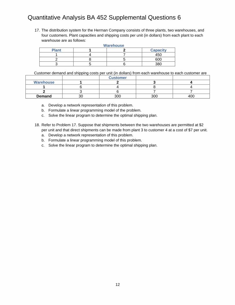
17. The distribution system for the Herman Company consists of three plants, two warehouses, and four customers. Plant capacities and shipping costs per unit (in dollars) from each plant to each warehouse are as follows:
Warehouse Plant 1 2 Capacity
1 4 7 450 2 8 5 600 3 5 6 380
Customer demand and shipping costs per unit (in dollars) from each warehouse to each customer are
Customer Warehouse 1 2 3 4
1 6 4 8 4 2 3 6 7 7
Demand 30 300 300 400
a. Develop a network representation of this problem. b. Formulate a linear programming model of the problem. c. Solve the linear program to determine the optimal shipping plan.
18. Refer to Problem 17. Suppose that shipments between the two warehouses are permitted at $2
per unit and that direct shipments can be made from plant 3 to customer 4 at a cost of $7 per unit. a. Develop a network representation of this problem. b. Formulate a linear programming model of this problem. c. Solve the linear program to determine the optimal shipping plan.

Quantitative Analysis BA 452 Supplemental Questions 6
13
19. Adirondack Paper Mills, Inc., operates paper plants in Augusta, Maine, and Tupper Lake, New York. Warehouse facilities are located in Albany, New York, and Portsmouth, New Hampshire. Distributors are located in Boston, New York, and Philadelphia. The plant capacities and distributor demands for the next month are as follows: Plant Capacity (units) Augusta 300 Tupper 100
Distributor Demand (units) Boston 150
New York 100 Philadelphia 150
The unit transportation costs (in dollars) for shipments from the two plants to the two warehouses and from the two warehouses to the three distributors are as follows:
a. Draw the network representation of the Adirondack Paper Mills problem. b. Formulate the Adirondack Paper Mills problem as a linear programming problem. c. Solve the linear program to determine the minimum cost shipping schedule for the problem.

Quantitative Analysis BA 452 Supplemental Questions 6
14
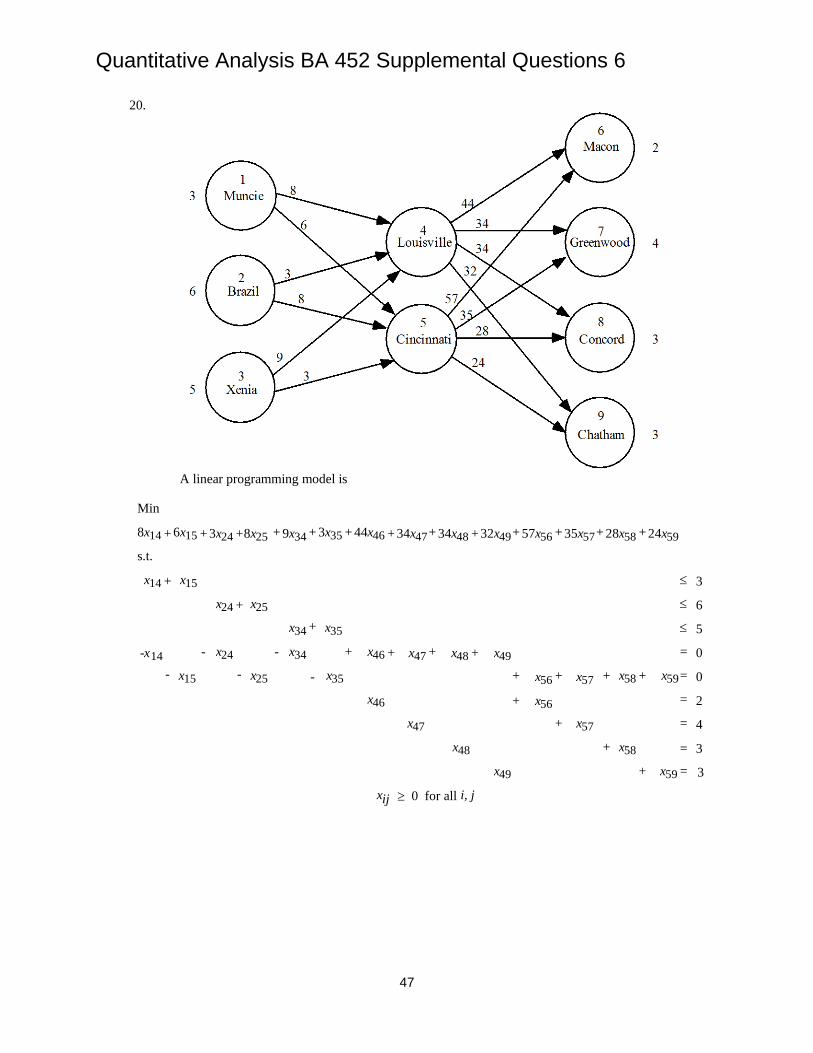
20. The Moore & Harman Company is in the business of buying and selling grain. An important aspect of the company’s business is arranging for the purchased grain to be shipped to customers. If the company can keep freight costs low, profitability will improve.
The company recently purchased three rail cars of grain at Muncie, Indiana; six rail cars at Brazil, Indiana; and five rail cars at Xenia, Ohio. Twelve carloads of grain have been sold. The locations and the amount sold at each location are as follows:
All shipments must be routed through either Louisville of Cincinnati. Shown are the shipping costs per bushel (incents) from the origins to Louisville and Cincinnati and the costs per bushel to ship from Louisville and Cincinnati to the destinations.
Determine a shipping schedule that will minimize the freight costs necessary to satisfy demand. Which (if any) rail cars of grain must be held at the origin until buyers can be found?
Quantitative Analysis BA 452 Supplemental Questions 6
15
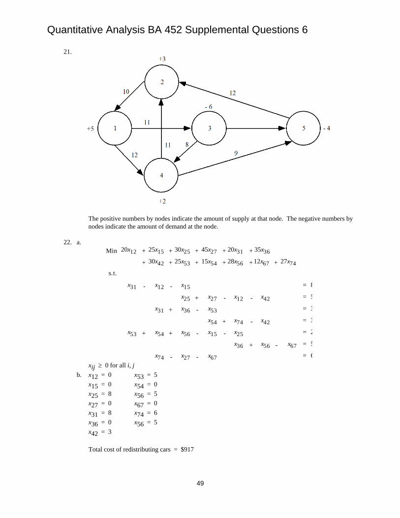
21. The following linear programming formulation is for a transshipment problem:
Show the network representation of this problem.
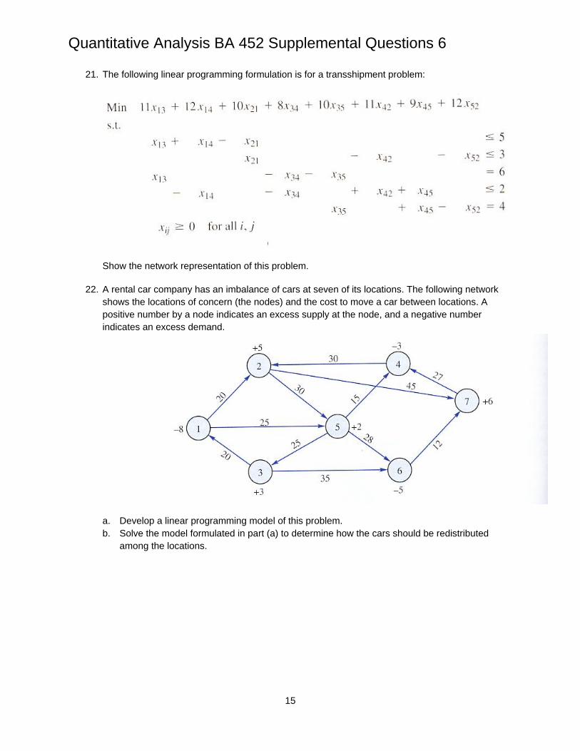
22. A rental car company has an imbalance of cars at seven of its locations. The following network
shows the locations of concern (the nodes) and the cost to move a car between locations. A positive number by a node indicates an excess supply at the node, and a negative number indicates an excess demand.
a. Develop a linear programming model of this problem. b. Solve the model formulated in part (a) to determine how the cars should be redistributed
among the locations.

Quantitative Analysis BA 452 Supplemental Questions 6
16
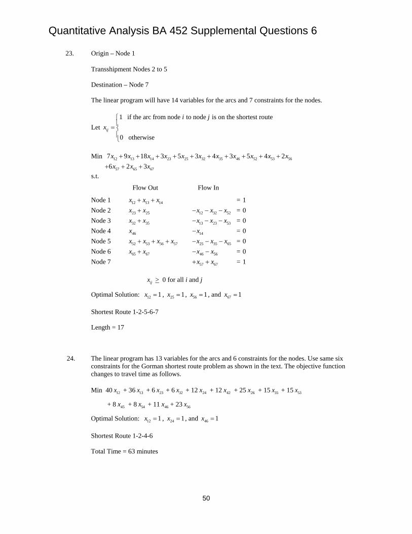
23. Find the shortest route from node 1 to node 7 in the network shown.
24. In the original Gorman Construction Company problem, we found the shortest distance from the
office (node 1) to the construction site located at node 6. Because some of the roads are highways and others are city streets, the shortest-distance routes between the office and the construction site may not necessarily provide the quickest of shortest-time route. Shown here is the Gorman road network with travel time rather than distance. Find the shortest route from Gorman’s office to the construction site at node 6 if the objective is to minimize travel time rather than distance.
Quantitative Analysis BA 452 Supplemental Questions 6
17
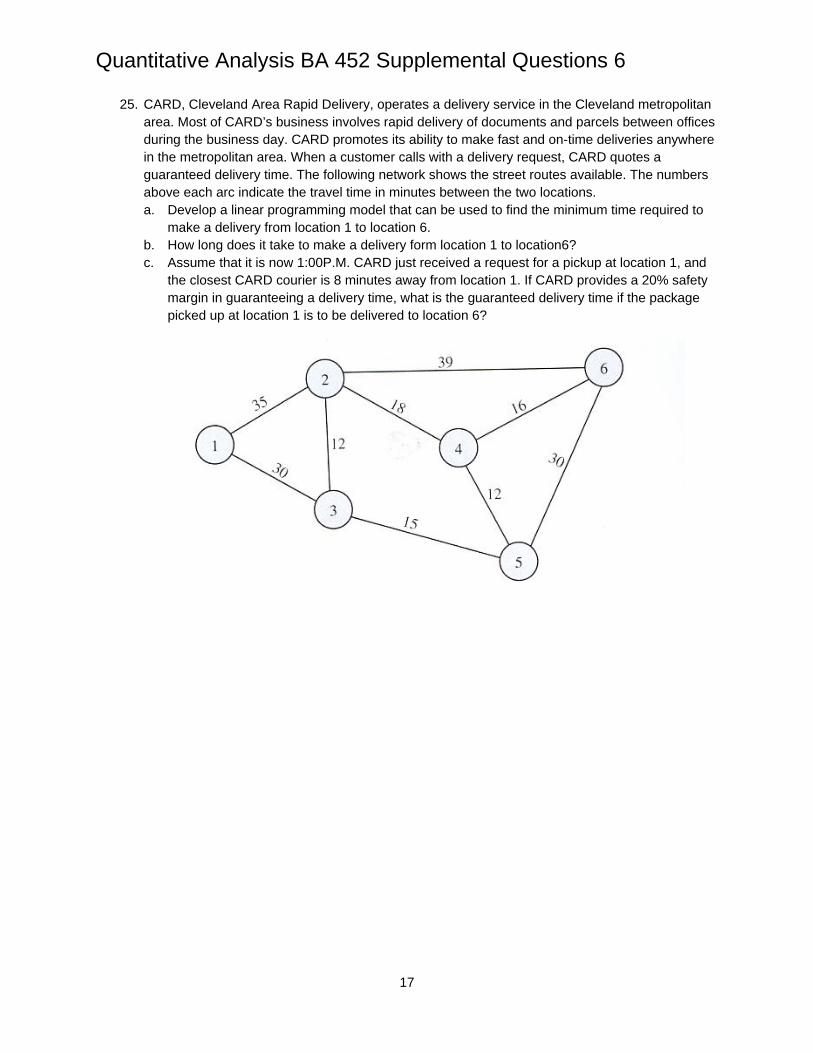
25. CARD, Cleveland Area Rapid Delivery, operates a delivery service in the Cleveland metropolitan area. Most of CARD’s business involves rapid delivery of documents and parcels between offices during the business day. CARD promotes its ability to make fast and on-time deliveries anywhere in the metropolitan area. When a customer calls with a delivery request, CARD quotes a guaranteed delivery time. The following network shows the street routes available. The numbers above each arc indicate the travel time in minutes between the two locations. a. Develop a linear programming model that can be used to find the minimum time required to
make a delivery from location 1 to location 6. b. How long does it take to make a delivery form location 1 to location6? c. Assume that it is now 1:00P.M. CARD just received a request for a pickup at location 1, and
the closest CARD courier is 8 minutes away from location 1. If CARD provides a 20% safety margin in guaranteeing a delivery time, what is the guaranteed delivery time if the package picked up at location 1 is to be delivered to location 6?

Quantitative Analysis BA 452 Supplemental Questions 6
18
26. Morgan Trucking Company operates a special pickup and delivery service between Chicago and six other cities located in a four-state area. When Morgan receives a request for service, it dispatches a truck from Chicago to the city requesting service as soon as possible. With both fast service and minimum travel costs as objectives for Morgan, it is important that the dispatched truck take the shortest route from Chicago to the specified city. Assume that the following network (not drawn to scale) with distances given in miles represents the highway network for this problem. Find the shortest-route distance from Chicago to node 6.
27. City Cab Company identified 10 primary pickup and drop locations for cab riders in New York City. In an effort to minimize travel time and improve customer service and the utilization of the company’s fleet of cabs, management would like the cab drivers to take the shortest route between locations whenever possible. Using the following network of roads and streets, what is the route a driver beginning at location 1 should take to reach location 10? The travel times in minutes are shown on the arcs of the network. Note that there are two one-way streets with the direction shown by the arrows.

Quantitative Analysis BA 452 Supplemental Questions 6
19
28. The five nodes in the following network represent points one year apart over a four-year period. Each node indicates a time when a decision is made to keep or replace a firm’s computer equipment. If a decision is made to replace the equipment, a decision must also be made as to how long the new equipment will be used. The arc from node 0 to node 1 represents the decision to keep the current equipment one year and replace it at the end of the year. The arc from node 0 to node 2 represents the decision to keep the current equipment two years and replace it at the end of year 2. The numbers above the arcs indicate the total cost associated with the equipment replacement decisions. These costs include discounted purchase price, trade-in value, operating costs, and maintenance costs. Use a shortest-route model to determine the minimum cost equipment replacement policy for the four-year period.
29. The north-south highway system passing through Albany, New York, can accommodate the capacities shown:
Can the highway system accommodate a north-south flow of 10,000 vehicles per hour?

Quantitative Analysis BA 452 Supplemental Questions 6
20
30. If the Albany highway system described in Problem 29 has revised flow capacities as shown in the following network, what is the maximal flow in vehicles per hour through the system? How many vehicles per hour must travel over each road (arc) to obtain this maximal flow?
31. A long-distance telephone company uses a fiber-optic network to transmit phone calls and other information between locations. Calls are carried through cable lines and switching nodes. A portion of the company’s transmission network is shown here. The numbers above each arc show the capacity in thousands of messages that can be transmitted over that branch of the network.
To keep up with the volume of information transmitted between origin and destination points, use the network to determine the maximum number of messages that may be sent from a city located at node 1 to a city located at node 7.
Quantitative Analysis BA 452 Supplemental Questions 6
21
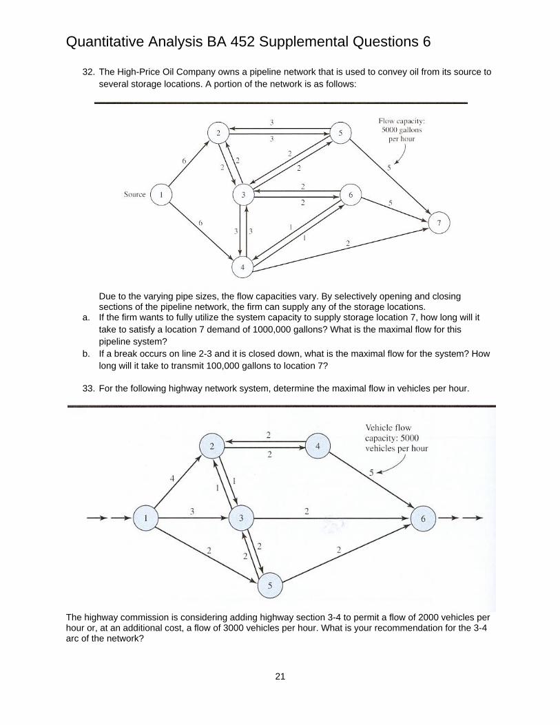
32. The High-Price Oil Company owns a pipeline network that is used to convey oil from its source to several storage locations. A portion of the network is as follows:
Due to the varying pipe sizes, the flow capacities vary. By selectively opening and closing sections of the pipeline network, the firm can supply any of the storage locations.
a. If the firm wants to fully utilize the system capacity to supply storage location 7, how long will it take to satisfy a location 7 demand of 1000,000 gallons? What is the maximal flow for this pipeline system?
b. If a break occurs on line 2-3 and it is closed down, what is the maximal flow for the system? How long will it take to transmit 100,000 gallons to location 7?
33. For the following highway network system, determine the maximal flow in vehicles per hour.
The highway commission is considering adding highway section 3-4 to permit a flow of 2000 vehicles per hour or, at an additional cost, a flow of 3000 vehicles per hour. What is your recommendation for the 3-4 arc of the network?
Quantitative Analysis BA 452 Supplemental Questions 6
22
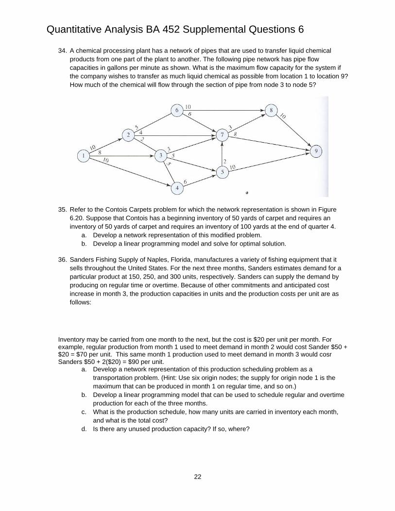
34. A chemical processing plant has a network of pipes that are used to transfer liquid chemical products from one part of the plant to another. The following pipe network has pipe flow capacities in gallons per minute as shown. What is the maximum flow capacity for the system if the company wishes to transfer as much liquid chemical as possible from location 1 to location 9? How much of the chemical will flow through the section of pipe from node 3 to node 5?
35. Refer to the Contois Carpets problem for which the network representation is shown in Figure 6.20. Suppose that Contois has a beginning inventory of 50 yards of carpet and requires an inventory of 50 yards of carpet and requires an inventory of 100 yards at the end of quarter 4.
a. Develop a network representation of this modified problem. b. Develop a linear programming model and solve for optimal solution.
36. Sanders Fishing Supply of Naples, Florida, manufactures a variety of fishing equipment that it
sells throughout the United States. For the next three months, Sanders estimates demand for a particular product at 150, 250, and 300 units, respectively. Sanders can supply the demand by producing on regular time or overtime. Because of other commitments and anticipated cost increase in month 3, the production capacities in units and the production costs per unit are as follows:
Inventory may be carried from one month to the next, but the cost is $20 per unit per month. For example, regular production from month 1 used to meet demand in month 2 would cost Sander $50 + $20 = $70 per unit. This same month 1 production used to meet demand in month 3 would cosr Sanders $50 + 2($20) = $90 per unit.
a. Develop a network representation of this production scheduling problem as a transportation problem. (Hint: Use six origin nodes; the supply for origin node 1 is the maximum that can be produced in month 1 on regular time, and so on.)
b. Develop a linear programming model that can be used to schedule regular and overtime production for each of the three months.
c. What is the production schedule, how many units are carried in inventory each month, and what is the total cost?
d. Is there any unused production capacity? If so, where?
Quantitative Analysis BA 452 Supplemental Questions 6
23
Answers to Supplemental Questions 6 1. The network model is shown.
Phila.
NewOrleans
Boston
Columbus
Dallas
Atlanta
5000
3000
7
5
21
2
6
6
2
1400
2000
3200
1400

Quantitative Analysis BA 452 Supplemental Questions 6
24
2. a. Let x11 : Amount shipped from Jefferson City to Des Moines x12 : Amount shipped from Jefferson City to Kansas City • • •
Min 14x11 + 9x12 + 7x13 + 8x21 + 10x22 + 5x23 s.t.
x11 + x12 + x13 ≤ 30 x21 + x22 + x23 ≤ 20 x11 + x21 = 25 x12 + x22 = 15 x13 + x23 = 10
x11, x12, x13, x21, x22, x23, ≥ 0
b. Optimal Solution:
Amount Cost Jefferson City - Des Moines 5 70 Jefferson City - Kansas City 15 135 Jefferson City - St. Louis 10 70 Omaha - Des Moines 20 160
Total 435
Quantitative Analysis BA 452 Supplemental Questions 6
25
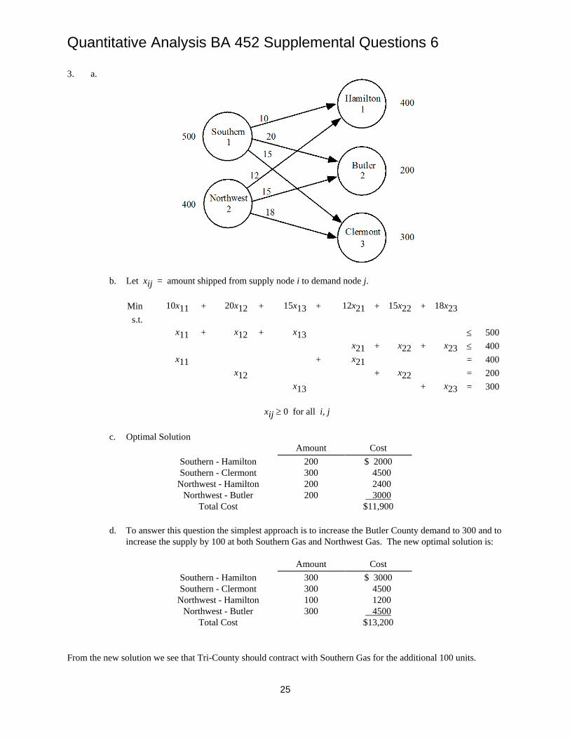
3. a.
b. Let xij = amount shipped from supply node i to demand node j.
Min 10x11 + 20x12 + 15x13 + 12x21 + 15x22 + 18x23 s.t.
x11 + x12 + x13 ≤ 500 x21 + x22 + x23 ≤ 400 x11 + x21 = 400 x12 + x22 = 200 x13 + x23 = 300
xij ≥ 0 for all i, j
c. Optimal Solution
Amount Cost Southern - Hamilton 200 $ 2000 Southern - Clermont 300 4500
Northwest - Hamilton 200 2400 Northwest - Butler 200 3000
Total Cost $11,900
d. To answer this question the simplest approach is to increase the Butler County demand to 300 and to increase the supply by 100 at both Southern Gas and Northwest Gas. The new optimal solution is:
Amount Cost
Southern - Hamilton 300 $ 3000 Southern - Clermont 300 4500
Northwest - Hamilton 100 1200 Northwest - Butler 300 4500
Total Cost $13,200
From the new solution we see that Tri-County should contract with Southern Gas for the additional 100 units.
Quantitative Analysis BA 452 Supplemental Questions 6
26
4. a.
b. The linear programming formulation and optimal solution are shown. The first two letters of the
variable name identify the “from” node and the second two letters identify the “to” node. LINEAR PROGRAMMING PROBLEM MIN 10SEPI + 20SEMO + 5SEDE + 9SELA + 10SEWA + 2COPI + 10COMO + 8CODE + 30COLA + 6COWA + 1NYPI + 20NYMO + 7NYDE + 10NYLA + 4NYWA S.T. 1) SEPI + SEMO + SEDE + SELA + SEWA <= 9000

Quantitative Analysis BA 452 Supplemental Questions 6
27
2) COPI + COMO + CODE + COLA + COWA <= 4000 3) NYPI + NYMO + NYDE + NYLA + NYWA <= 8000 4) SEPI + COPI + NYPI = 3000 5) SEMO + COMO + NYMO = 5000 6) SEDE + CODE + NYDE = 4000 7) SELA + COLA + NYLA = 6000 8) SEWA + COWA + NYWA = 3000 OPTIMAL SOLUTION
Optimal Objective Value 150000.00000
Variable Value Reduced Cost
SEPI 0.00000 10.00000 SEMO 0.00000 1.00000 SEDE 4000.00000 0.00000 SELA 5000.00000 0.00000 SEWA 0.00000 7.00000 COPI 0.00000 11.00000
COMO 4000.00000 0.00000 CODE 0.00000 12.00000 COLA 0.00000 30.00000 COWA 0.00000 12.00000 NYPI 3000.00000 0.00000
NYMO 1000.00000 0.00000 NYDE 0.00000 1.00000 NYLA 1000.00000 0.00000 NYWA 3000.00000 0.00000
Constraint Slack/Surplus Dual Value 1 0.00000 -1.00000 2 0.00000 -10.00000 3 0.00000 0.00000 4 0.00000 1.00000 5 0.00000 20.00000 6 0.00000 6.00000 7 0.00000 10.00000 8 0.00000 4.00000
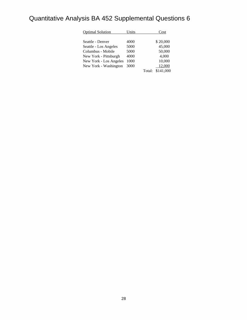
c. The new optimal solution actually shows a decrease of $9000 in shipping cost. It is summarized.
Quantitative Analysis BA 452 Supplemental Questions 6
28
Optimal Solution Units Cost Seattle - Denver 4000 $ 20,000 Seattle - Los Angeles 5000 45,000 Columbus - Mobile 5000 50,000 New York - Pittsburgh 4000 4,000 New York - Los Angeles 1000 10,000 New York - Washington 3000 12,000 Total: $141,000
Quantitative Analysis BA 452 Supplemental Questions 6
29
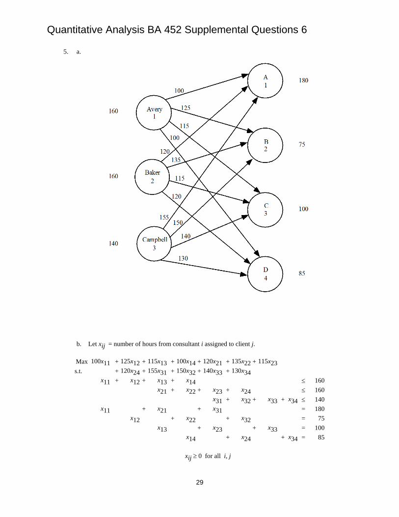
5. a.
b. Let xij = number of hours from consultant i assigned to client j.
Max 100x11 + 125x12 + 115x13 + 100x14 + 120x21 + 135x22 + 115x23 s.t. + 120x24 + 155x31 + 150x32 + 140x33 + 130x34 x11 + x12 + x13 + x14 ≤ 160 x21 + x22 + x23 + x24 ≤ 160 x31 + x32 + x33 + x34 ≤ 140 x11 + x21 + x31 = 180 x12 + x22 + x32 = 75 x13 + x23 + x33 = 100 x14 + x24 + x34 = 85
xij ≥ 0 for all i, j

Quantitative Analysis BA 452 Supplemental Questions 6
30
Optimal Solution Hours
Assigned
Billing Avery - Client B 40 $ 5,000 Avery - Client C 100 11,500 Baker - Client A 40 4,800 Baker - Client B 35 4,725 Baker - Client D 85 10,200
Campbell - Client A 140 21,700 Total Billing $57,925
c. New Optimal Solution
Hours Assigned
Billing
Avery - Client A 40 $ 4,000 Avery - Client C 100 11,500 Baker - Client B 75 10,125 Baker - Client D 85 10,200
Campbell - Client A 140 21,700 Total Billing $57,525

Quantitative Analysis BA 452 Supplemental Questions 6
31
6. The network model, the linear programming formulation, and the optimal solution are shown. Note that the third constraint corresponds to the dummy origin. The variables x31, x32, x33, and x34 are the amounts shipped out of the dummy origin; they do not appear in the objective function since they are given a coefficient of zero.
Max 32x11 34x12+ + 32x13 40x14+ 34x21 30x22 28x23 38x24++++
s.t.
x11 x12+ + x13
x21 x22+ + x23
x31 x32+ + x33
≤ 5000
3000
4000
2000
5000
3000=
=
=
≤
≤
= 2000
Dummy
x31+
x32+
+ x33
x21+
x22+
+ x23
x11
x12
x13
x14+
x24+
+ x34
x14 x24+ + x34
xij ≥ 0 for all i, j
C.S.
D.
Dum
D1
D2
D3
D4
0
0
00
40
32
34
32
38
28
3034
5000
3000
4000
3000
5000
2000
2000
Supply
Demand
Note: Dummy origin has supply of 4000.
Quantitative Analysis BA 452 Supplemental Questions 6
32
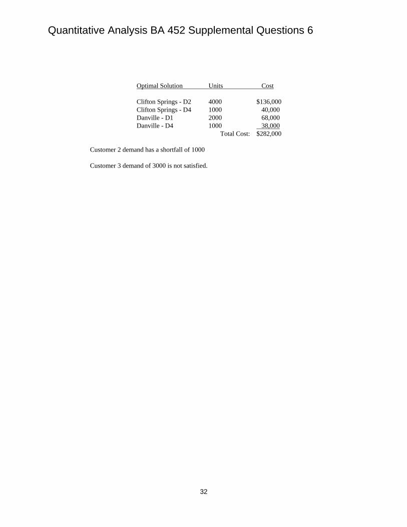
Optimal Solution Units Cost Clifton Springs - D2 4000 $136,000 Clifton Springs - D4 1000 40,000 Danville - D1 2000 68,000 Danville - D4 1000 38,000 Total Cost: $282,000 Customer 2 demand has a shortfall of 1000 Customer 3 demand of 3000 is not satisfied.

Quantitative Analysis BA 452 Supplemental Questions 6
33
7. a.
b. There are alternative optimal solutions.
Solution #1 Solution # 2 Denver to St. Paul: 10
Denver to St. Paul: 10
Atlanta to Boston: 50 Atlanta to Boston: 50 Atlanta to Dallas: 50 Atlanta to Los Angeles: 50 Chicago to Dallas: 20 Chicago to Dallas: 70 Chicago to Los Angeles: 60 Chicago to Los Angeles: 10 Chicago to St. Paul: 70 Chicago to St. Paul: 70 Total Profit: $4240
If solution #1 is used, Forbelt should produce 10 motors at Denver, 100 motors at Atlanta, and 150 motors at Chicago. There will be idle capacity for 90 motors at Denver.
If solution #2 is used, Forbelt should adopt the same production schedule but a modified shipping
schedule.
Los3
3
Chicago
2Atlanta
1
Denver
2
Dallas
1
Boston
4St. Paul
16
13
188
13
8
11
7
10
12
1720
100
100
150
60
70
80
50
Angeles
My answer to this homework question will go here. To find your answer, you may want to study the answers to some of the similar questions.
Quantitative Analysis BA 452 Supplemental Questions 6
34
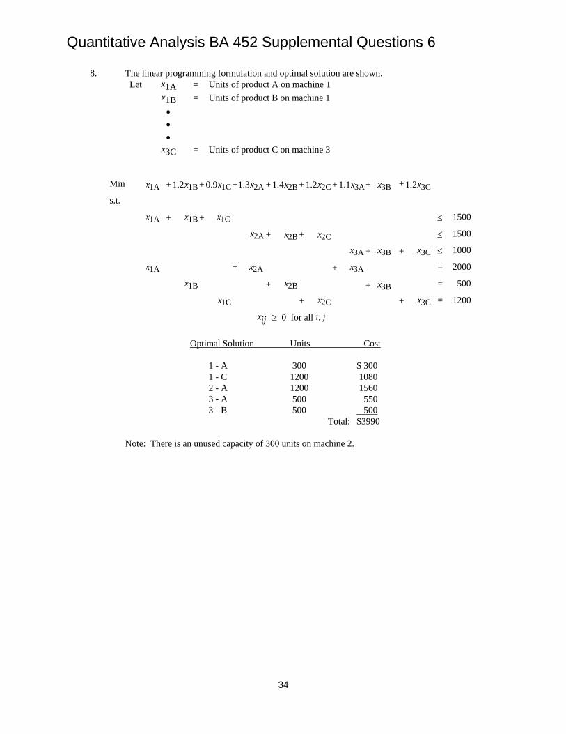
8. The linear programming formulation and optimal solution are shown. Let x1A = Units of product A on machine 1 x1B = Units of product B on machine 1 • • • x3C = Units of product C on machine 3
Min x1A 1.2x1B+ + 0.9x1C 1.3x2A+ 1.4x2B 1.2x2C 1.1x3A x3B++++
s.t.
x1A x1B+ + x1C
x2A x2B+ + x2Cx3A x3B+ + x3C
≤ 1500
1500
1000
2000
500
1200=
=
=
≤
≤
x3A+
x3B+
+ x3C
x2A+
x2B+
+ x2C
x1A
x1B
x1C
1.2x3C+
xij ≥ 0 for all i, j Optimal Solution Units Cost 1 - A 300 $ 300 1 - C 1200 1080 2 - A 1200 1560 3 - A 500 550 3 - B 500 500 Total: $3990 Note: There is an unused capacity of 300 units on machine 2.
Quantitative Analysis BA 452 Supplemental Questions 6
35
9. a.
b.
Min 10x11 + 16x12 + 32x13 + 14x21 + 22x22 + 40x23 + 22x31 + 24x32 + 34x33 s.t. x11 + x12 + x13 ≤ 1 x21 + x22 + x23 ≤ 1 x31 + x32 + x33 ≤ 1 x11 + x21 + x31 = 1 x12 + x22 + x32 = 1 x13 + x23 + x33 = 1
xij ≥ 0 for all i, j Solution x12 = 1, x21 = 1, x33 = 1 Total completion time = 64
Quantitative Analysis BA 452 Supplemental Questions 6
36
10. a.
b.
Min 30x11 + 44x12 + 38x13 + 47x14 + 31x15 + 25x21 + + 28x55 s.t. x11 + x12 + x13 + x14 + x15 ≤ 1 x21 + x22 + x23 + x24 + x25 ≤ 1 x31 + x32 + x33 + x34 + x35 ≤ 1 x41 + x42 + x43 + x44 + x45 ≤ 1 x51 + x52 + x53 + x54 + x55 ≤ 1 x11 + x21 + x31 + x41 + x51 = 1 x12 + x22 + x32 + x42 + x52 = 1 x13 + x23 + x33 + x43 + x53 = 1 x14 + x24 + x34 + x44 + x54 = 1 x15 + x25 + x35 + x45 + x55 = 1
xij ≥ 0, i = 1, 2,.., 5; j = 1, 2,.., 5 Optimal Solution:
Green to Job 1 $26 Brown to Job 2 34 Red to Job 3 38 Blue to Job 4 39 White to Job 5 25 $162
Since the data is in hundreds of dollars, the total installation cost for the 5 contracts is $16,200.
Quantitative Analysis BA 452 Supplemental Questions 6
37
11. This can be formulated as a linear program with a maximization objective function. There are 24 variables, one for each program/time slot combination. There are 10 constraints, 6 for the potential programs and 4 for the time slots.
Optimal Solution: NASCAR Live 5:00 – 5:30 p.m. Hollywood Briefings 5:30 – 6:00 p.m. World News 7:00 – 7:30 p.m. Ramundo & Son 8:00 – 8:30 p.m. Total expected advertising revenue = $30,500
My answer to this homework question will go here. To find your answer, you may want to study the answers to some of the similar questions.

Quantitative Analysis BA 452 Supplemental Questions 6
38
12. a. This is the variation of the assignment problem in which multiple assignments are possible. Each distribution center may be assigned up to 3 customer zones.
The linear programming model of this problem has 40 variables (one for each combination of
distribution center and customer zone). It has 13 constraints. There are 5 supply (≤ 3) constraints and 8 demand (= 1) constraints.
The optimal solution is given below.
Assignments Cost ($1000s) Plano: Kansas City, Dallas 34 Flagstaff: Los Angeles 15 Springfield: Chicago, Columbus, Atlanta 70 Boulder: Newark, Denver 97 Total Cost - $216
b. The Nashville distribution center is not used. c. All the distribution centers are used. Columbus is switched from Springfield to Nashville. Total
cost increases by $11,000 to $227,000.
Quantitative Analysis BA 452 Supplemental Questions 6
39
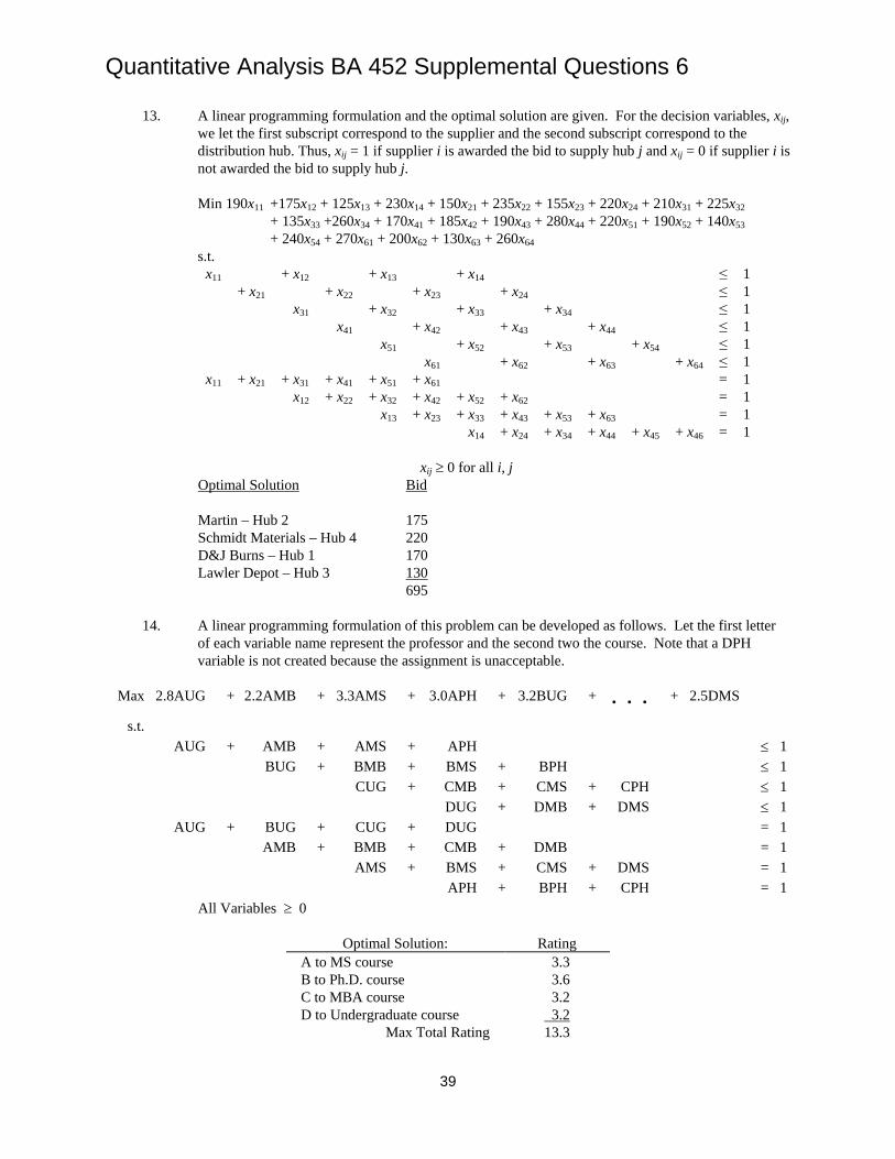
13. A linear programming formulation and the optimal solution are given. For the decision variables, xij, we let the first subscript correspond to the supplier and the second subscript correspond to the distribution hub. Thus, xij = 1 if supplier i is awarded the bid to supply hub j and xij = 0 if supplier i is not awarded the bid to supply hub j.
Min 190x11 +175x12 + 125x13 + 230x14 + 150x21 + 235x22 + 155x23 + 220x24 + 210x31 + 225x32
+ 135x33 +260x34 + 170x41 + 185x42 + 190x43 + 280x44 + 220x51 + 190x52 + 140x53 + 240x54 + 270x61 + 200x62 + 130x63 + 260x64
s.t. x11 + x12 + x13 + x14 ≤ 1
+ x21 + x22 + x23 + x24 ≤ 1 x31 + x32 + x33 + x34 ≤ 1 x41 + x42 + x43 + x44 ≤ 1 x51 + x52 + x53 + x54 ≤ 1 x61 + x62 + x63 + x64 ≤ 1
x11 + x21 + x31 + x41 + x51 + x61 = 1 x12 + x22 + x32 + x42 + x52 + x62 = 1 x13 + x23 + x33 + x43 + x53 + x63 = 1 x14 + x24 + x34 + x44 + x45 + x46 = 1
xij ≥ 0 for all i, j
Optimal Solution Bid Martin – Hub 2 175 Schmidt Materials – Hub 4 220 D&J Burns – Hub 1 170 Lawler Depot – Hub 3 130 695
14. A linear programming formulation of this problem can be developed as follows. Let the first letter
of each variable name represent the professor and the second two the course. Note that a DPH variable is not created because the assignment is unacceptable.
Max 2.8AUG + 2.2AMB + 3.3AMS + 3.0APH + 3.2BUG + · · · + 2.5DMS
s.t. AUG + AMB + AMS + APH ≤ 1 BUG + BMB + BMS + BPH ≤ 1 CUG + CMB + CMS + CPH ≤ 1 DUG + DMB + DMS ≤ 1 AUG + BUG + CUG + DUG = 1 AMB + BMB + CMB + DMB = 1 AMS + BMS + CMS + DMS = 1 APH + BPH + CPH = 1
All Variables ≥ 0
Optimal Solution: Rating A to MS course 3.3 B to Ph.D. course 3.6 C to MBA course 3.2 D to Undergraduate course 3.2
Max Total Rating 13.3

Quantitative Analysis BA 452 Supplemental Questions 6
40
15. a. Min 150x11 + 210x12 + 270x13
+ 170x21 + 230x22 + 220x23 + 180x31 + 230x32 + 225x33 + 160x41 + 240x42 + 230x43
s.t. x11 + x12 + x13 ≤ 1 x21 + x22 + x23 ≤ 1 x31 + x32 + x33 ≤ 1 x41 + x42 + x43 ≤ 1 x11 +x21 +x31 +x41 = 1 x12 +x22 +x32 +x42 = 1 x13 +x23 +x33 +x43 = 1
xij ≥ for all i, j
Optimal Solution: x12 = 1, x23 = 1, x41 = 1 Total hours required: 590 Note: statistician 3 is not assigned. b. The solution will not change, but the total hours required will increase by 5. This is the extra time
required for statistician 4 to complete the job for client A. c. The solution will not change, but the total time required will decrease by 20 hours. d. The solution will not change; statistician 3 will not be assigned. Note that this occurs because
increasing the time for statistician 3 makes statistician 3 an even less attractive candidate for assignment.
My answer to this homework question will go here. To find your answer, you may want to study the answers to some of the similar questions.
Quantitative Analysis BA 452 Supplemental Questions 6
41
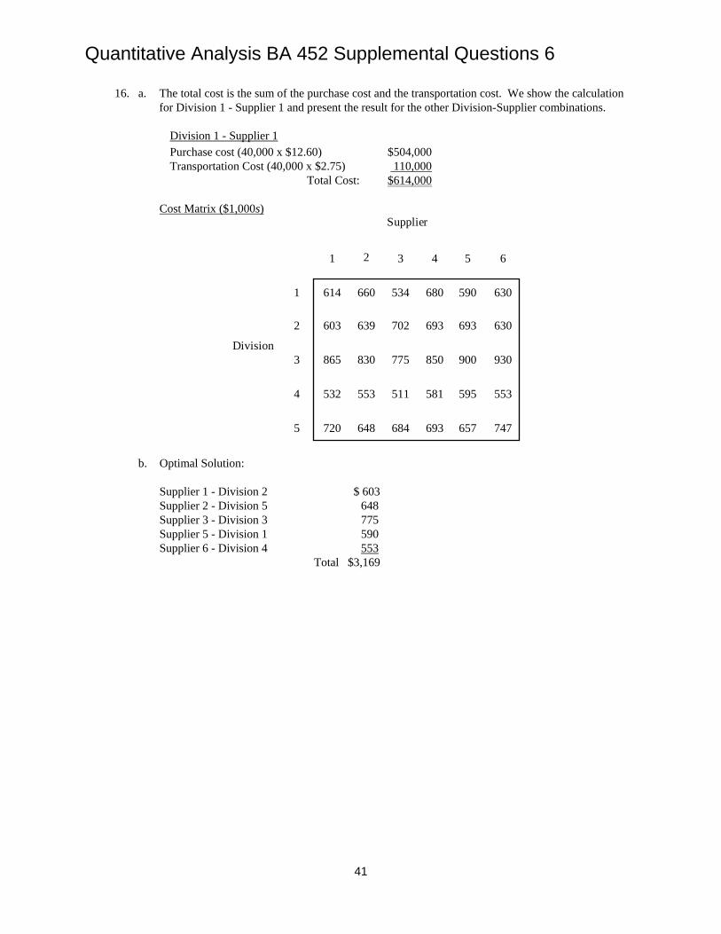
16. a. The total cost is the sum of the purchase cost and the transportation cost. We show the calculation for Division 1 - Supplier 1 and present the result for the other Division-Supplier combinations.
Division 1 - Supplier 1 Purchase cost (40,000 x $12.60) $504,000 Transportation Cost (40,000 x $2.75) 110,000
Total Cost: $614,000
Cost Matrix ($1,000s)
b. Optimal Solution: Supplier 1 - Division 2 $ 603 Supplier 2 - Division 5 648 Supplier 3 - Division 3 775 Supplier 5 - Division 1 590 Supplier 6 - Division 4 553 Total $3,169
Supplier
Division
1
2
3
4
5
1 2 3 4 5 6
614
603
865
532
720
660
639
830
553
648
534
702
775
511
684
680
693
850
581
693
590
693
900
595
657
630
630
930
553
747
Quantitative Analysis BA 452 Supplemental Questions 6
42
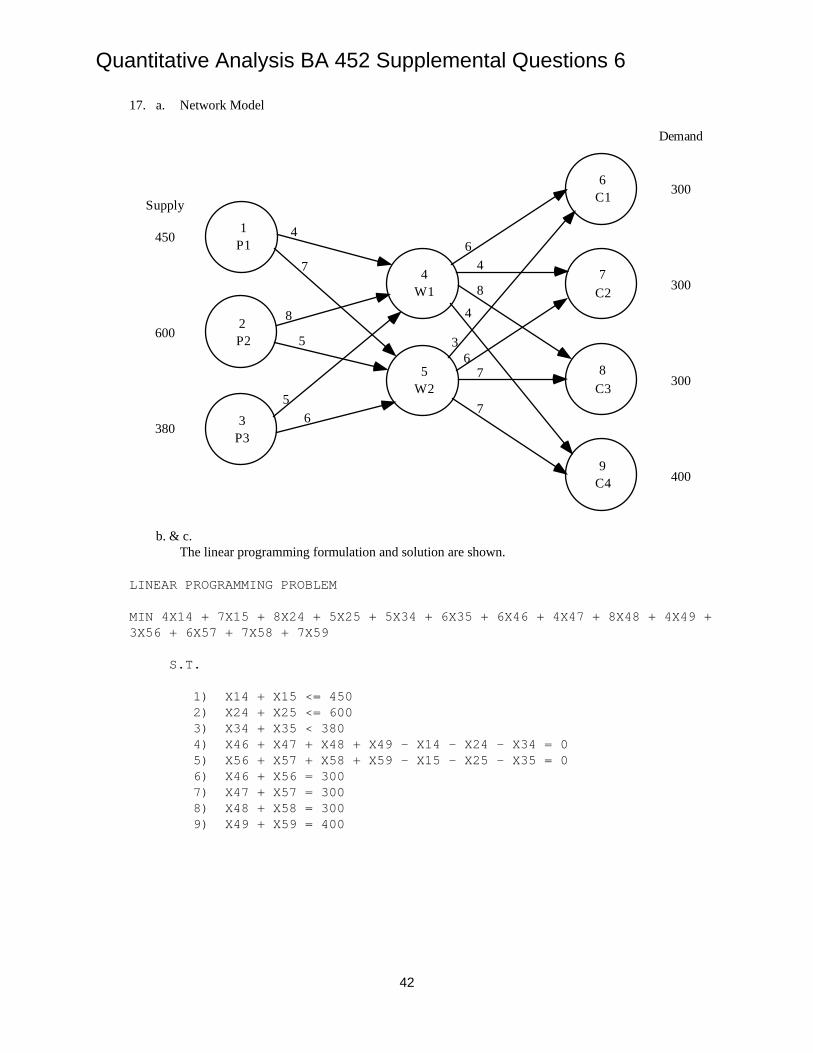
17. a. Network Model
b. & c. The linear programming formulation and solution are shown. LINEAR PROGRAMMING PROBLEM MIN 4X14 + 7X15 + 8X24 + 5X25 + 5X34 + 6X35 + 6X46 + 4X47 + 8X48 + 4X49 + 3X56 + 6X57 + 7X58 + 7X59 S.T. 1) X14 + X15 <= 450 2) X24 + X25 <= 600 3) X34 + X35 < 380 4) X46 + X47 + X48 + X49 - X14 - X24 - X34 = 0 5) X56 + X57 + X58 + X59 - X15 - X25 - X35 = 0 6) X46 + X56 = 300 7) X47 + X57 = 300 8) X48 + X58 = 300 9) X49 + X59 = 400
1P1
3P3
8C3
9C4
4W1
7C2
5W2
6C1
2P2
4
7
8
5
56
64
8
4
36
7
7
Supply
450
600
380
Demand
300
300
300
400

Quantitative Analysis BA 452 Supplemental Questions 6
43
OPTIMAL SOLUTION
Optimal Objective Value 11850.00000
Variable Value Reduced Cost
X14 450.00000 0.00000 X15 0.00000 2.00000 X24 0.00000 4.00000 X25 600.00000 0.00000 X34 250.00000 0.00000 X35 0.00000 0.00000 X46 0.00000 2.00000 X47 300.00000 0.00000 X48 0.00000 0.00000 X49 400.00000 0.00000 X56 300.00000 0.00000 X57 0.00000 3.00000 X58 300.00000 0.00000 X59 0.00000 4.00000
Constraint Slack/Surplus Dual Value 1 0.00000 -1.00000 2 0.00000 -1.00000 3 130.00000 0.00000 4 0.00000 9.00000 5 0.00000 9.00000 6 0.00000 13.00000 7 0.00000 9.00000 8 0.00000 5.00000 9 0.00000 6.00000
There is an excess capacity of 130 units at plant 3.
Quantitative Analysis BA 452 Supplemental Questions 6
44
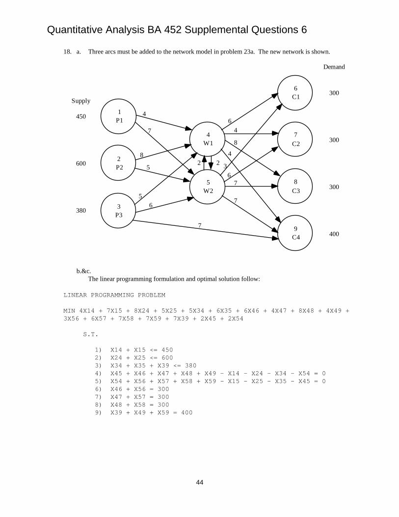
18. a. Three arcs must be added to the network model in problem 23a. The new network is shown.
b.&c. The linear programming formulation and optimal solution follow: LINEAR PROGRAMMING PROBLEM MIN 4X14 + 7X15 + 8X24 + 5X25 + 5X34 + 6X35 + 6X46 + 4X47 + 8X48 + 4X49 + 3X56 + 6X57 + 7X58 + 7X59 + 7X39 + 2X45 + 2X54 S.T. 1) X14 + X15 <= 450 2) X24 + X25 <= 600 3) X34 + X35 + X39 <= 380 4) X45 + X46 + X47 + X48 + X49 - X14 - X24 - X34 - X54 = 0 5) X54 + X56 + X57 + X58 + X59 - X15 - X25 - X35 - X45 = 0 6) X46 + X56 = 300 7) X47 + X57 = 300 8) X48 + X58 = 300 9) X39 + X49 + X59 = 400
1P1
3P3
8C3
9C4
4W1
7C2
5W2
6C1
2P2
4
7
8
5
56
64
8
4
36
7
7
Supply
450
600
380
Demand
300
300
300
400
22
7
Quantitative Analysis BA 452 Supplemental Questions 6
45
OPTIMAL SOLUTION
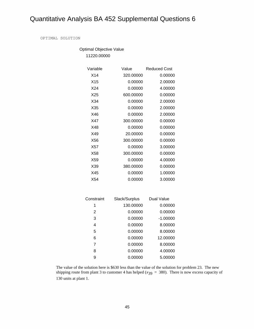
Optimal Objective Value 11220.00000
Variable Value Reduced Cost
X14 320.00000 0.00000 X15 0.00000 2.00000 X24 0.00000 4.00000 X25 600.00000 0.00000 X34 0.00000 2.00000 X35 0.00000 2.00000 X46 0.00000 2.00000 X47 300.00000 0.00000 X48 0.00000 0.00000 X49 20.00000 0.00000 X56 300.00000 0.00000 X57 0.00000 3.00000 X58 300.00000 0.00000 X59 0.00000 4.00000 X39 380.00000 0.00000 X45 0.00000 1.00000 X54 0.00000 3.00000
Constraint Slack/Surplus Dual Value 1 130.00000 0.00000 2 0.00000 0.00000 3 0.00000 -1.00000 4 0.00000 8.00000 5 0.00000 8.00000 6 0.00000 12.00000 7 0.00000 8.00000 8 0.00000 4.00000 9 0.00000 5.00000
The value of the solution here is $630 less than the value of the solution for problem 23. The new
shipping route from plant 3 to customer 4 has helped (x39 = 380). There is now excess capacity of 130 units at plant 1.

Quantitative Analysis BA 452 Supplemental Questions 6
46
19. a.
b.
Min 7x13 + 5x14 + 3x23 + 4x24 + 8x35 + 5x36 + 7x37 + 5x45 + 6x46 + 10x47 s.t.
x13 + x14 ≤ 300 x23 + x24 ≤ 100 -x13 - x23 + x35 + x36 + x37 = 0 - x14 - x24 + x45 + x46 + x47 = 0 x35 + x45 = 150 + x36 + x46 = 100 x37 + x47 = 150
xij ≥ 0 for all i and j
c. Optimal Solution: Variable Value x13 50 x14 250 x23 100 x24 0 x35 0 x36 0 x37 150 x45 150 x46 100 x47 0 Objective Function: 4300
3Albany
4Portsmouth
8
5
7
56
107
Philadelphia
6NewYork
5Boston 150
100
150
7
5
34
2Tupper Lake
1Augusta300
100
My answer to this homework question will go here. To find your answer, you may want to study the answers to some of the similar questions.
Quantitative Analysis BA 452 Supplemental Questions 6
47
20.
A linear programming model is
Min
8x14 6x15+ + 3x24 8x25+ 9x34 3x35+ 44x46+ 34x47 34x48 32x49++ ++ 57x56+ 35x57+ 28x58+ 24x59+
s.t.
x14 x15+
=
=
=
≤
≤
≤
= 3
3
4
2
0
0
5
6
3
=
=
x24 x25+
x34 x35+
-x14
x15-
x24- - x34
- x35
x46+ x47 x48 x49++ +
x46
x47
x48
x49
x56+ x57+ x58+ x59+
x56x57
x58
x59
xij ≥ 0 for all i, j
- x25
+
+
+
+
Quantitative Analysis BA 452 Supplemental Questions 6
48
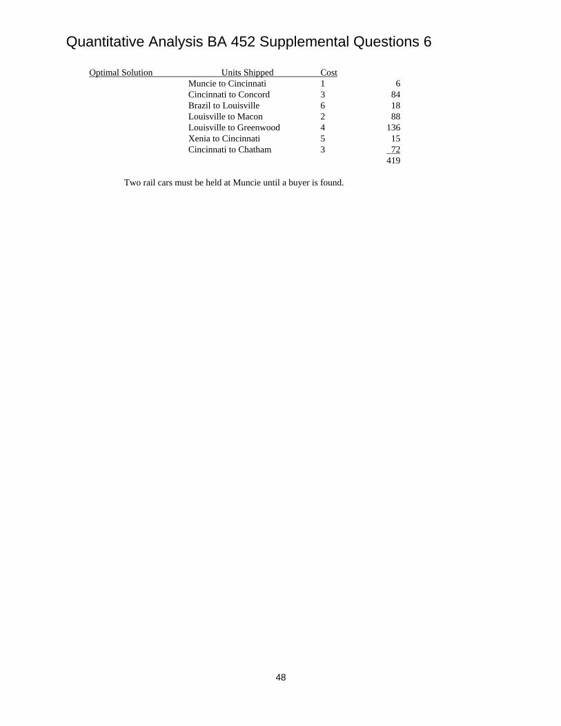
Optimal Solution Units Shipped Cost Muncie to Cincinnati 1 6 Cincinnati to Concord 3 84 Brazil to Louisville 6 18 Louisville to Macon 2 88 Louisville to Greenwood 4 136 Xenia to Cincinnati 5 15 Cincinnati to Chatham 3 72 419 Two rail cars must be held at Muncie until a buyer is found.
Quantitative Analysis BA 452 Supplemental Questions 6
49
21.
The positive numbers by nodes indicate the amount of supply at that node. The negative numbers by
nodes indicate the amount of demand at the node. 22. a.
xij ≥ 0 for all i, j b. x12 = 0 x53 = 5 x15 = 0 x54 = 0 x25 = 8 x56 = 5 x27 = 0 x67 = 0 x31 = 8 x74 = 6 x36 = 0 x56 = 5 x42 = 3 Total cost of redistributing cars = $917
Min
s.t.
20x12 + 25x15
30x42
x12
x31
x54
x74
-
+
+
-
x15
x25
x36
x56
x27
+
-
-
-
x27
x53
x54
x15
x67
-
+
-
x12
x74
x25
x36
-
-
+
x42
x42
x56 - x67
x31 -
x53 +
= 8
= 5
= 3
= 3
= 2
= 5
= 6
+
+
30x25
25x53
+
+
45x27
15x54
+
+
20x31
28x56
+
+
35x36
12x67 + 27x74+
Quantitative Analysis BA 452 Supplemental Questions 6
50
23. Origin – Node 1 Transshipment Nodes 2 to 5 Destination – Node 7 The linear program will have 14 variables for the arcs and 7 constraints for the nodes.
Let 1 if the arc from node to node is on the shortest route
0 otherwiseij
i jx
=
Min 12 13 14 23 25 32 35 46 52 53 567 9 18 3 5 3 4 3 5 4 2x x x x x x x x x x x+ + + + + + + + + + 57 65 676 2 3x x x+ + + s.t.
Flow Out Flow In
Node 1 12 13 14x x x+ + = 1 Node 2 23 25x x+ 12 32 52x x x− − − = 0 Node 3 32 35x x+ 13 23 53x x x− − − = 0 Node 4 46x 14x− = 0 Node 5 52 53 56 57x x x x+ + + 25 35 65x x x− − − = 0 Node 6 65 67x x+ 46 56x x− − = 0 Node 7 57 67x x+ + = 1 ijx > 0 for all i and j
Optimal Solution: 12 1x = , 25 1x = , 56 1x = , and 67 1x = Shortest Route 1-2-5-6-7 Length = 17 24. The linear program has 13 variables for the arcs and 6 constraints for the nodes. Use same six
constraints for the Gorman shortest route problem as shown in the text. The objective function changes to travel time as follows.
Min 40 12x + 36 13x + 6 23x + 6 32x + 12 24x + 12 42x + 25 26x + 15 35x + 15 53x
+ 8 45x + 8 54x + 11 46x + 23 56x
Optimal Solution: 12 1x = , 24 1x = , and 46 1x = Shortest Route 1-2-4-6 Total Time = 63 minutes
Quantitative Analysis BA 452 Supplemental Questions 6
51
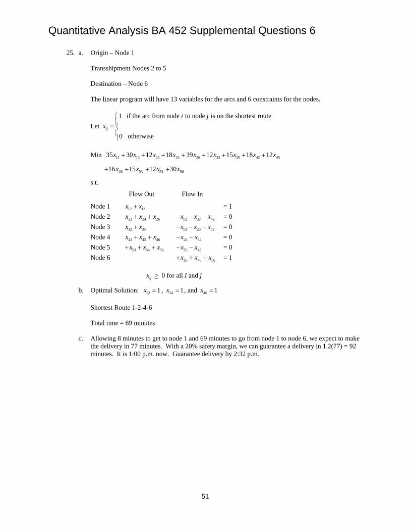
25. a. Origin – Node 1 Transshipment Nodes 2 to 5 Destination – Node 6 The linear program will have 13 variables for the arcs and 6 constraints for the nodes.
Let 1 if the arc from node to node is on the shortest route
0 otherwiseij
i jx
=
Min 12 13 23 24 26 32 35 42 4535 30 12 18 39 12 15 18 12x x x x x x x x x+ + + + + + + +
4616x+ 5315x+ 5412x+ 5630x+
s.t.
Flow Out Flow In
Node 1 12 13x x+ = 1 Node 2 23 24 26x x x+ + 12 32 42x x x− − − = 0 Node 3 32 35x x+ 13 23 53x x x− − − = 0 Node 4 42 45 46x x x+ + 24 54x x− − = 0 Node 5 53 54 56x x x+ + + 35 45x x− − = 0 Node 6 26 46 56x x x+ + + = 1 ijx > 0 for all I and j
b. Optimal Solution: 12 1x = , 24 1x = , and 46 1x = Shortest Route 1-2-4-6 Total time = 69 minutes c. Allowing 8 minutes to get to node 1 and 69 minutes to go from node 1 to node 6, we expect to make
the delivery in 77 minutes. With a 20% safety margin, we can guarantee a delivery in 1.2(77) = 92 minutes. It is 1:00 p.m. now. Guarantee delivery by 2:32 p.m.
Quantitative Analysis BA 452 Supplemental Questions 6
52
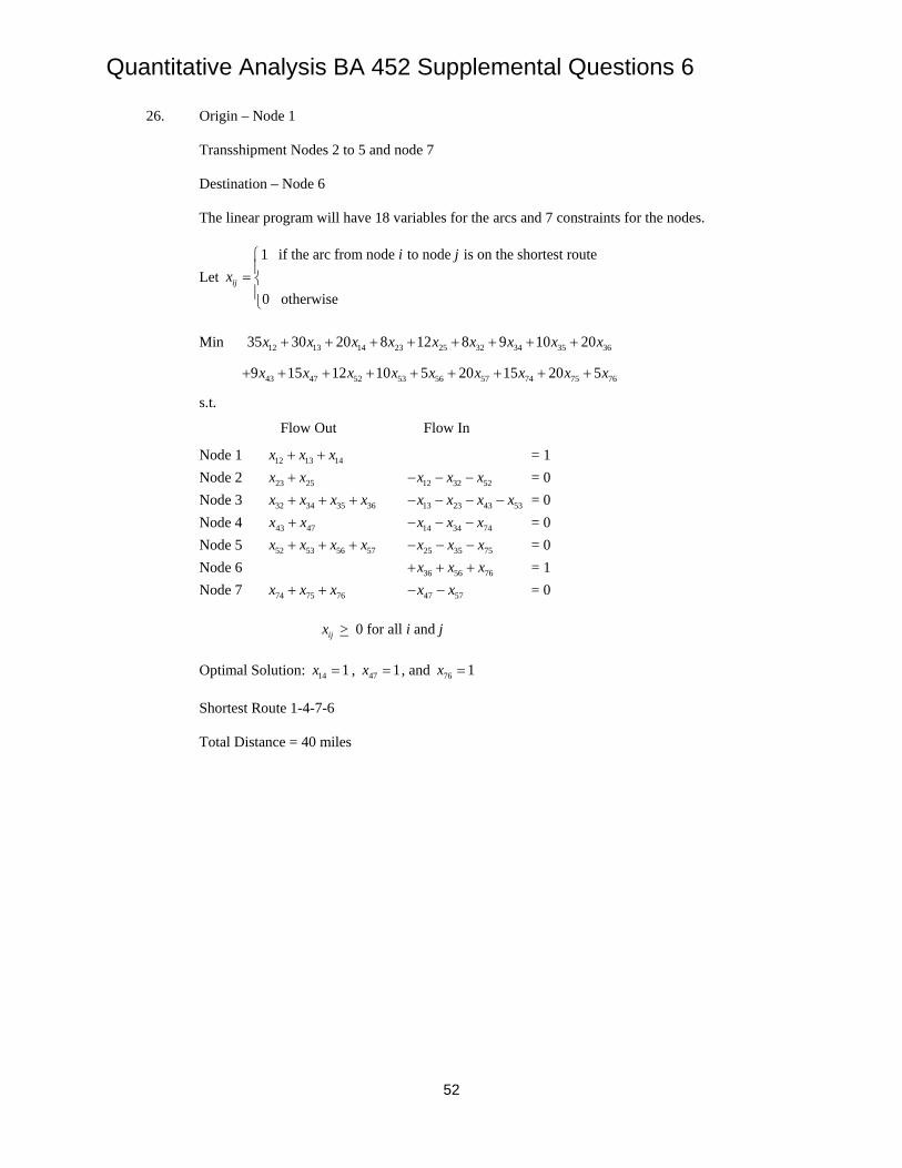
26. Origin – Node 1 Transshipment Nodes 2 to 5 and node 7 Destination – Node 6 The linear program will have 18 variables for the arcs and 7 constraints for the nodes.
Let 1 if the arc from node to node is on the shortest route
0 otherwiseij
i jx
=
Min 12 13 14 23 25 32 34 35 3635 30 20 8 12 8 9 10 20x x x x x x x x x+ + + + + + + +
43 47 52 53 56 57 74 75 769 15 12 10 5 20 15 20 5x x x x x x x x x+ + + + + + + + +
s.t.
Flow Out Flow In
Node 1 12 13 14x x x+ + = 1 Node 2 23 25x x+ 12 32 52x x x− − − = 0 Node 3 32 34 35 36x x x x+ + + 13 23 43 53x x x x− − − − = 0 Node 4 43 47x x+ 14 34 74x x x− − − = 0 Node 5 52 53 56 57x x x x+ + + 25 35 75x x x− − − = 0 Node 6 36 56 76x x x+ + + = 1 Node 7 74 75 76x x x+ + 47 57x x− − = 0 ijx > 0 for all i and j Optimal Solution: 14 1x = , 47 1x = , and 76 1x = Shortest Route 1-4-7-6 Total Distance = 40 miles

Quantitative Analysis BA 452 Supplemental Questions 6
53
27. Origin – Node 1 Transshipment Nodes 2 to 9 Destination – Node 10 (Identified by the subscript 0) The linear program will have 29 variables for the arcs and 10 constraints for the nodes.
Let 1 if the arc from node to node is on the shortest route
0 otherwiseij
i jx
=
Min 12 13 14 15 23 27 32 36 43 458 13 15 10 5 15 5 5 2 4x x x x x x x x x x+ + + + + + + + + 46 54 59 63 64 67 68 69 72 763 4 12 5 3 4 2 5 15 4x x x x x x x x x x+ + + + + + + + + + 78 70 86 89 80 95 96 98 902 4 2 5 7 12 5 5 5x x x x x x x x x+ + + + + + + + +
s.t.
Flow Out Flow In
Node 1 12 13 14 15x x x x+ + + = 1 Node 2 23 27x x+ 12 32 72x x x− − − = 0 Node 3 32 36x x+ 13 23 43 63x x x x− − − − = 0 Node 4 43 45 46x x x+ + 14 54 64x x x− − − = 0 Node 5 54 59x x+ 15 45 95x x x− − − = 0 Node 6 63 64 67 68 69x x x x x+ + + + 36 46 76 86 96x x x x x− − − − − = 0 Node 7 72 76 78 70x x x x+ + + 27 67x x− − = 0 Node 8 86 89 80x x x+ + 68 78 98x x x− − − = 0 Node 9 95 96 98 90x x x x+ + + 59 69 89x x x− − − = 0 Node 10 70 80 90x x x+ + + = 1 ijx > 0 for all i and j
Optimal Solution: 15 1x = , 54 1x = , 46 1x = , 67 1x = , and 70 1x = Shortest Route 1-5-4-6-7-10 Total Time = 25 minutes
Quantitative Analysis BA 452 Supplemental Questions 6
54
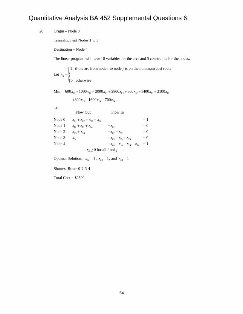
28. Origin – Node 0 Transshipment Nodes 1 to 3 Destination – Node 4 The linear program will have 10 variables for the arcs and 5 constraints for the nodes.
Let 1 if the arc from node to node is on the minimum cost route
0 otherwiseij
i jx
=
Min 01 02 03 04 12 13 14600 1000 2000 2800 500 1400 2100x x x x x x x+ + + + + +
23 24 34800 1600 700x x x+ + +
s.t. Flow Out Flow In
Node 0 01 02 03 04x x x x+ + + = 1 Node 1 12 13 14x x x+ + 01x− = 0 Node 2 23 24x x+ 02 12x x− − = 0 Node 3 34x 03 13 23x x x− − − = 0 Node 4 04 14 24 34x x x x− − − − = 1 ijx > 0 for all i and j
Optimal Solution: 02 1x = , 23 1x = , and 34 1x = Shortest Route 0-2-3-4 Total Cost = $2500

Quantitative Analysis BA 452 Supplemental Questions 6
55
29. The capacitated transshipment problem to solve is given: Max x61 s.t. x12 + x13 + x14 - x61 = 0 x24 + x25 - x12 - x42 = 0 x34 + x36 - x13 - x43 = 0 x42 + x43 + x45 + x46 - x14 - x24 - x34 - x54 = 0 x54 + x56 - x25 - x45 = 0 x61 - x36 + x46 - x56 = 0 x12 ≤ 2 x13 ≤ 6 x14 ≤ 3 x24 ≤ 1 x25 ≤ 4 x34 ≤ 3 x36 ≤ 2 x42 ≤ 1 x43 ≤ 3 x45 ≤ 1 x46 ≤ 3 x54 ≤ 1 x56 ≤ 6 xij ≥ 0 for all i, j
4
5
6
2
3
1
2
3
11
3
4 2 2
3
4
Maximum Flow 9,000 Vehicles Per Hour
The system cannot accommodate a flow of 10,000 vehicles per hour.

Quantitative Analysis BA 452 Supplemental Questions 6
56
30.
31. The maximum number of messages that may be sent is 10,000. 32. a. 10,000 gallons per hour or 10 hours b. Flow reduced to 9,000 gallons per hour; 11.1 hours. 33. Current Max Flow = 6,000 vehicles/hour. With arc 3-4 at a 3,000 unit/hour flow capacity, total system flow is increased to 8,000
vehicles/hour. Increasing arc 3-4 to 2,000 units/hour will also increase system to 8,000 vehicles/hour. Thus a 2,000 unit/hour capacity is recommended for this arc.
34. Maximal Flow = 23 gallons / minute. Five gallons will flow from node 3 to node 5.
4
5
6
2
3
1
3
4
21
3
5 3 2
3
6
11,000

Quantitative Analysis BA 452 Supplemental Questions 6
57
35. a. Modify the problem by adding two nodes and two arcs. Let node 0 be a beginning inventory node with a supply of 50 and an arc connecting it to node 5 (period 1 demand). Let node 9 be an ending inventory node with a demand of 100 and an arc connecting node 8 (period 4 demand to it).
b.
Min + 2x15 + 5x26 + 3x37 + 3x48 + 0.25x56 + 0.25x67 + 0.25x78 + 0.25x89 s.t. x05 = 50 x15 ≤ 600 x26 ≤ 300 x37 ≤ 500 x48 ≤ 400 x05 + x15 - x56 = 400 x26 + x56 - x67 = 500 x37 + x67 - x78 = 400 x48 + x78 - x89 = 400 x89 = 100
xij ≥ 0 for all i and j Optimal Solution: x05 = 50 x56 = 250 x15 = 600 x67 = 0 x26 = 250 x78 = 100 x37 = 500 x89 = 100 x48 = 400 Total Cost = $5262.50
Quantitative Analysis BA 452 Supplemental Questions 6
58
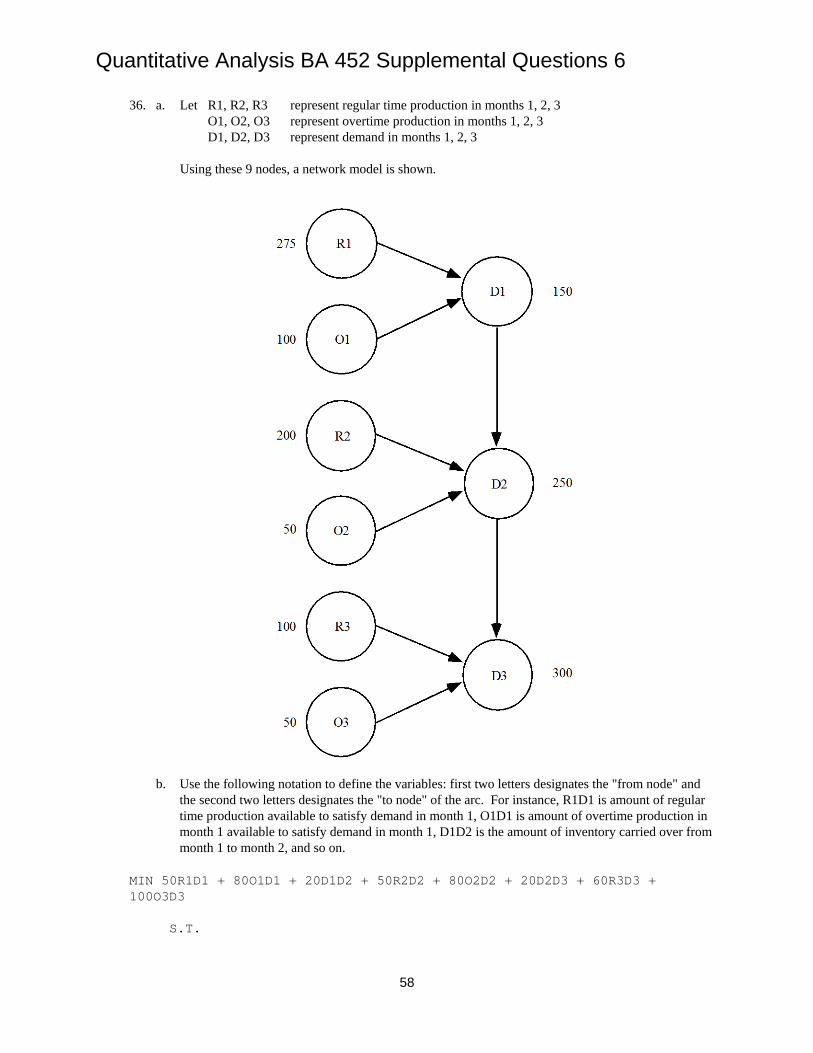
36. a. Let R1, R2, R3 represent regular time production in months 1, 2, 3 O1, O2, O3 represent overtime production in months 1, 2, 3 D1, D2, D3 represent demand in months 1, 2, 3 Using these 9 nodes, a network model is shown.
b. Use the following notation to define the variables: first two letters designates the "from node" and the second two letters designates the "to node" of the arc. For instance, R1D1 is amount of regular time production available to satisfy demand in month 1, O1D1 is amount of overtime production in month 1 available to satisfy demand in month 1, D1D2 is the amount of inventory carried over from month 1 to month 2, and so on.
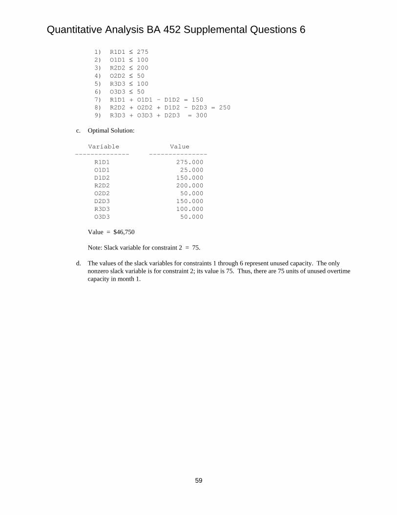
MIN 50R1D1 + 80O1D1 + 20D1D2 + 50R2D2 + 80O2D2 + 20D2D3 + 60R3D3 + 100O3D3 S.T.
Quantitative Analysis BA 452 Supplemental Questions 6
59
1) R1D1 ≤ 275 2) O1D1 ≤ 100 3) R2D2 ≤ 200 4) O2D2 ≤ 50 5) R3D3 ≤ 100 6) O3D3 ≤ 50 7) R1D1 + O1D1 - D1D2 = 150 8) R2D2 + O2D2 + D1D2 - D2D3 = 250 9) R3D3 + O3D3 + D2D3 = 300 c. Optimal Solution: Variable Value -------------- --------------- R1D1 275.000 O1D1 25.000 D1D2 150.000 R2D2 200.000 O2D2 50.000 D2D3 150.000 R3D3 100.000 O3D3 50.000 Value = $46,750 Note: Slack variable for constraint 2 = 75. d. The values of the slack variables for constraints 1 through 6 represent unused capacity. The only
nonzero slack variable is for constraint 2; its value is 75. Thus, there are 75 units of unused overtime capacity in month 1.


