QPAC Overview Report

QPAC: Quintessa’s

General-Purpose Modelling

Software

QRS-QPAC-11

June 2013

QRS-QPAC-11, June 2013

Quintessa Limited Tel: +44 (0) 1491 636246 The Hub, 14 Station Road Fax: +44 (0) 1491 636247 Henley-on-Thames [email protected] Oxfordshire RG9 1AY www.quintessa.org United Kingdom www.quintessa-online.com

Document History

Title: QPAC: Quintessa’s General-Purpose Modelling Software

Document Number: QRS-QPAC-11

Date: June 2013

Prepared by: Philip Maul

Reviewed by: Claire Watson

Approved by: Claire Watson


i

Summary

QPAC is a general-purpose modelling tool developed by Quintessa. It can be used to

solve a wide range of problems, including those with strongly coupled nonlinear

processes, at resolutions varying from high-level systems models to detailed

research-level models. QPAC uses a flexible ‘model as input’ approach that allows the

user to define the processes to be included in any calculation, by inputting the

equations to be solved in addition to any input parameters and the system

discretisation. Traditional modelling software has the mathematical model hardwired

into the code, making it difficult to add new processes or extend existing ones: QPAC

makes this easy.

Once a process has been modelled and fully tested, it can be wrapped as a QPAC

module to allow it to be reused. In this way, QPAC can operate in a mode more akin

to traditional modelling software, where the only inputs required from the modeller

are the input parameters, boundary conditions and system discretisation. However,

QPAC differs from traditional software by making the coupling of additional processes

to an existing module straightforward.

QPAC is an in-house software tool that enables Quintessa to provide modelling

support to its clients. QPAC Player enables small applications with graphical user

interfaces to be produced that can be used by others to run QPAC simulations and

perform sensitivity studies. In addition, QPAC can be used as a rapid prototyping tool

and models built in QPAC can subsequently form the basis of bespoke software for use

in specific technical areas.

In this document a general overview is given of the capabilities of the software

together with examples of its use in the fields of energy and the environment. QPAC

has been used for geochemical modelling, flow and transport modelling and for

problems involving coupled thermal, hydraulic, mechanical and chemical (THMC)

processes. It has been used to solve problems in the fields of geologic storage of carbon

dioxide, the evolution of engineered barrier systems in geological disposal facilities for

radioactive waste and the behaviour of graphite in gas-cooled nuclear reactors.


iii

Contents

1 Introduction 1

2 Fundamental Concepts 2

2.1 Types of Modelling 2

2.2 Rapid Prototyping 4

2.3 QPAC Player and Viewer 6

3 Carbon Dioxide in the Terrestrial Environment 9

3.1 A Site with Naturally High CO2 Surface Fluxes 9

3.2 Systems Modelling of Terrestrial Storage Sites 12

3.3 Detailed Modelling of Cement Well Seals 14

3.4 Detailed Modelling of Two-Phase Flow 14

4 Geochemical Modelling 16

4.1 A Natural Clay System in Alkaline Conditions 16

4.2 Iron-Bentonite Systems 19

4.3 The Tournemire Industrial Analogue 21

5 Fluid Flow and Transport 24

5.1 Repository Resaturation Calculations 24

5.2 Gas Flow in Disposal Facilities and the FORGE Project 26

5.3 Gas Flow through Graphite 32

6 THMC Modelling 35

6.1 The THERESA Project 35

6.1.1 Benchmarking Test Cases 35

6.1.2 The Canister Retrieval Test 37

6.2 The DECOVALEX Project 40

References 42

Appendix A : Technical Details 45

A.1 System Discretisation 45

A.2 Process Models and Variables 46

A.3 The Finite Volume Method 47

A.4 A Simple Example: Heat Conduction 49

Appendix B : Quality Assurance 51


1

1 Introduction

Traditionally, software designed for mathematical modelling is targeted at a specific

problem and has the equations hardwired into the code. The user provides input

parameters, the system geometry, boundary conditions and the discretisation scheme.

However, this approach has a number of drawbacks:

1. It is difficult to make changes to the underlying conceptual models; a software

engineer is required and, depending on how the source code is written, it may

be laborious to make the required changes.

2. Different models (realised in different pieces of software) cannot be linked

together easily; often only crude coupling can be represented, with output from

one piece of software providing input to another.

3. Only those parameters and options that the software designer has chosen to

expose to the user can be edited.

4. The conceptual model may often be a ‘black box’, or at least only as well

understood as the accompanying documentation permits.

Modern general-purpose modelling tools go some way to providing solutions to these

problems. QPAC, developed by Quintessa, is one such tool. It can be used to solve a

wide range of problems, including those with strongly coupled nonlinear processes, at

resolutions varying from high-level systems models to detailed research-level models.

QPAC uses a flexible ‘model as input’ approach that allows the user to define the

processes to be included in any calculation, by inputting the equations to be solved in

addition to any input parameters and the details of system discretisation. QPAC

makes adding new processes or extending existing ones easy.

QPAC is an in-house software tool that enables Quintessa to provide modelling

support to its clients. QPAC Player enables small applications with graphical user

interfaces to be produced that can be used by others to run QPAC simulations and

perform sensitivity studies. In addition, QPAC can be used as a rapid prototyping tool

and models built in QPAC can subsequently form the basis of bespoke software for use

in specific technical areas.

This document gives an overview of QPAC, starting with key concepts in the use of the

software in Section 2, with some of the technical details being discussed in more detail

in Appendix A. The remainder of this document describes a number of areas where

QPAC has been applied, illustrating how the software has been used by Quintessa to

address complex problems in the fields of energy and the environment. It is only

possible to give a summary of these here, but interested readers can find further details

in the referenced published papers. QPAC has been developed under the TickIT

quality assurance scheme. Quality assurance issues are discussed in Appendix B.


2

2 Fundamental Concepts

QPAC can be used to model complex systems that evolve with time. In QPAC all

quantities can be time dependent.

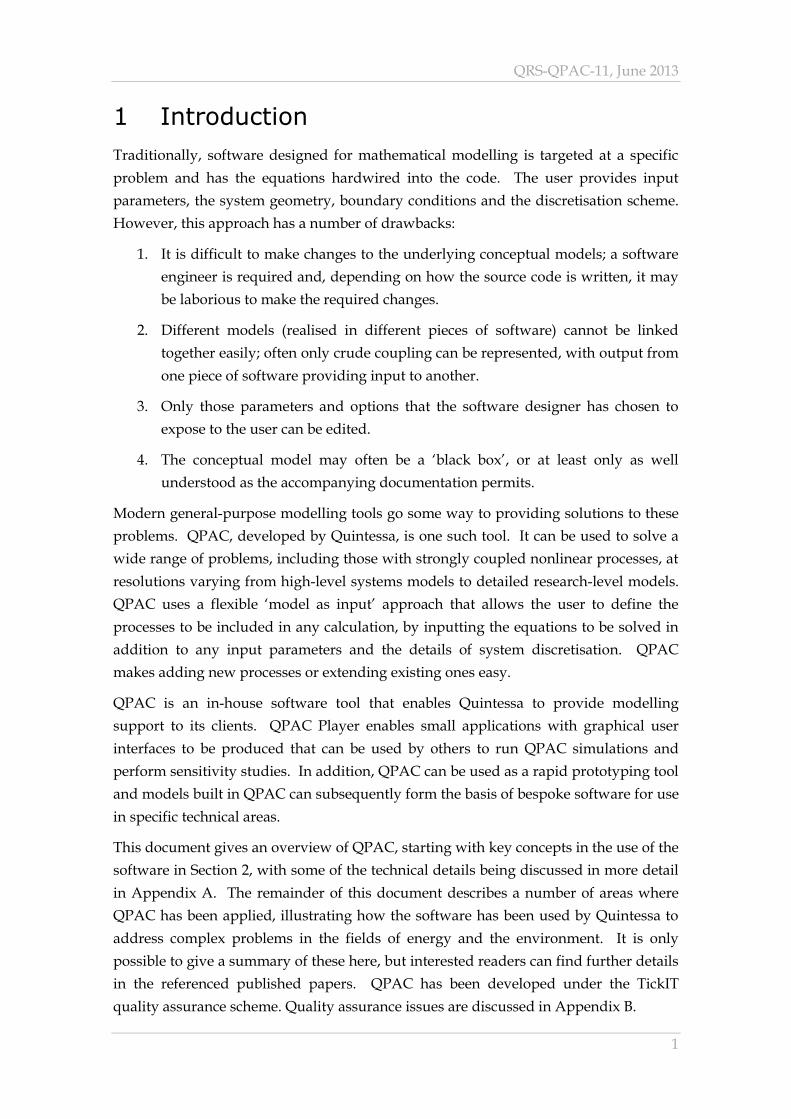
In QPAC a system represents the entire modelling domain. This may be comprised of

a number of subsystems, each representing a distinct part of the domain where

different processes may occur. Each system or subsystem is broken down into a

number of compartments (sometimes referred to as control volumes), which may be

arranged in a geometric grid (or grids), as illustrated in Figure 1. In fact both ‘free’

compartments and grids can be used together. Although QPAC does not impose the

approach that is to be used for spatially discretising the system, the finite volume (or

control volume) approach is generally used, as described in Appendix A.

Figure 1: An example QPAC grid

The most important QPAC capability is to be able to add new processes to a model.

Previously it was necessary to produce new pieces of software, or force old software to

learn ‘new tricks’; this could be time-consuming and would often be hindered by

design decisions taken in the development of the codes. To overcome these difficulties

QPAC has been developed so that the model equations are part of the input, allowing

new processes to be added straightforwardly – the ‘model as input’ philosophy.

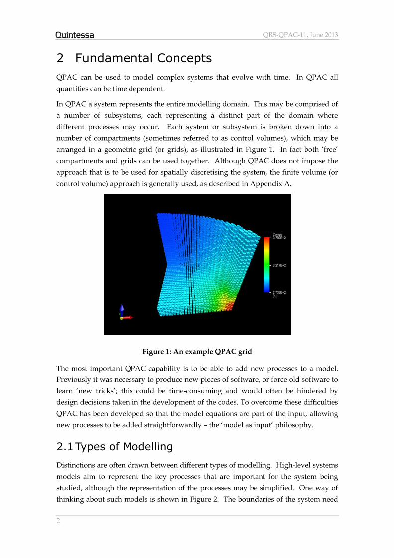
2.1 Types of Modelling

Distinctions are often drawn between different types of modelling. High-level systems

models aim to represent the key processes that are important for the system being

studied, although the representation of the processes may be simplified. One way of

thinking about such models is shown in Figure 2. The boundaries of the system need


3

to be defined and it may be appropriate to split the system up into a number of

interacting subsystems. Features, Events and Processes (FEPs) relevant to the system

can be described, and it is useful to distinguish between FEPs that are external to the

system (EFEPs) and those that are internal to the system. The EFEPs can combine to

generate scenarios for system evolution. In systems modelling the processes to be

modelled are represented in a ‘top down’ way.

Figure 2: Systems modelling

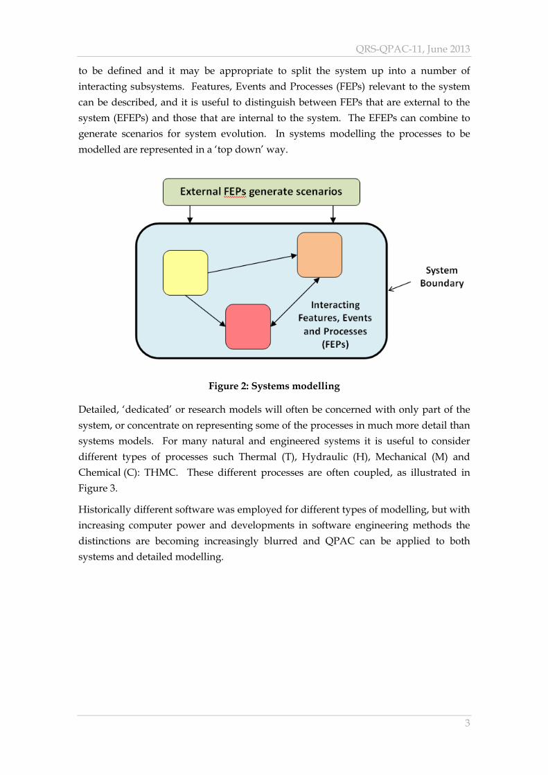
Detailed, ‘dedicated’ or research models will often be concerned with only part of the

system, or concentrate on representing some of the processes in much more detail than

systems models. For many natural and engineered systems it is useful to consider

different types of processes such Thermal (T), Hydraulic (H), Mechanical (M) and

Chemical (C): THMC. These different processes are often coupled, as illustrated in

Figure 3.

Historically different software was employed for different types of modelling, but with

increasing computer power and developments in software engineering methods the

distinctions are becoming increasingly blurred and QPAC can be applied to both

systems and detailed modelling.


4

Figure 3: An example of THMC process coupling

2.2 Rapid Prototyping

The ability to add new processes when needed makes QPAC an ideal tool for rapid

prototyping. The key processes can be represented and a simulation for the system

being studied produced much more rapidly than with traditional codes.

Built-in units checking and conversion is another feature of QPAC that speeds up the

development of simulations. All quantities must have specified units with compatible

units (e.g. metres and feet) being automatically converted. When working in areas

where mixtures of units are used this feature is invaluable. Where the use of

incompatible units is identified, an error message is produced and the simulation halts.

Once a model for specified processes has been developed it can be ‘wrapped’ to enable

it to be re-used in other applications - this is called a module. QPAC modules can often

be used to facilitate rapid prototyping; they can provide the starting point for

representing relevant processes even if the finally-produced software requires

modified versions to be employed. The use of modules exemplifies of code re-use

which speeds up software development and contributes to good quality assurance.

The modules that are currently employed by Quintessa include:

Thermal processes. This is a comparatively simple module where the standard

equations for heat conduction, convection and radiation are implemented.


5

Multiphase phase flow (MPF). Several modules for the representation of fluid

flow in porous media have been developed. The 'classic' multiphase flow

relationships effectively assume a well-mixed disposition of fluids with the

relative permeability for a compartment being isotropic. This approach is applied

where the saturation changes over length scales large in comparison with the grid

size. An alternative conceptual model is that used for large-scale groundwater

flow modelling, where the fluids are assumed to be poorly mixed and there is a

distinct 'free-surface'. This conceptual model is typically used where the grid size

is large in comparison with the length scale over which the saturation changes and

where capillary effects are of secondary importance.

Tracer transport. In conjunction with fluid flow calculations, modelling the

transport of trace materials or contaminants is often required. The processes in the

tracer transport module include: advection with dispersion; diffusion; equilibrium

sorption; solubility limitation; and radioactive decay and ingrowth. Matrix

diffusion is a special case of the diffusion process; it is generally modelled as a one-

dimensional process perpendicular to the flow direction along a fracture.

Reactive transport. This module is designed to simulate the chemical interactions

of groundwater and other subsurface fluids with rocks and manmade materials.

These interactions play an important role in both fundamental geological

processes and the evolution of engineered structures. In an open system the

interactions in the water-rock system are represented by reactive transport

equations, which couple the fluid flow equations to those representing the

geochemical reactions between the porewater components and the solid materials.

The equations are fully coupled in the sense that alteration processes in the rock

and manmade materials feed back into the fluid flow through variations in

porosity and other material properties such as permeability and tortuosity.

Mechanical processes. This module allows the representation of classical small-

strain elastic deformations for both transient (e.g. pressure waves) and

instantaneous static analyses. The module supports non-linear elasticity,

orthotropic anisotropy, poro-elasticity and thermo-elasticity. In addition, the

module allows the user to specify arbitrary non-elastic strains, providing the

capability to include customised elastic-plastic or visco-elastic models. The

Mohr-Coulomb failure model, modified cam-clay model and various ‘creep’

models have all been used successfully with this module.


6

2.3 QPAC Player and Viewer

Once a satisfactory (although necessarily simplified) understanding of system

evolution has been obtained, decisions can be taken on whether further software

development is needed. If repeated calculations with different input parameters are

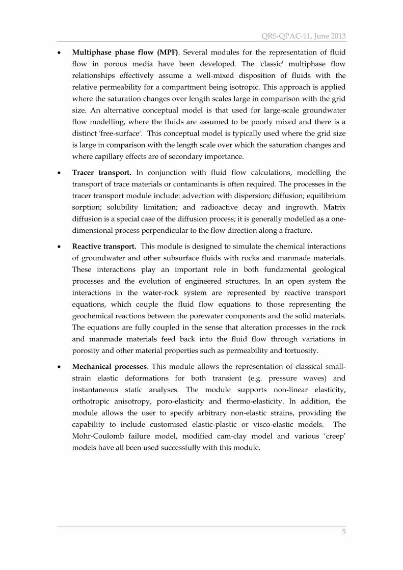
likely to be needed, one option is to produce a QPAC Player version of the application.

A QPAC Player version provides a simple graphical user interface that enables end

users to change key input parameters without being exposed to the full complexity of

the underlying process models. Figure 4 gives an example of the user interface for a

hydrological sediment compaction model. Parameter input is by a combination of

input boxes and sliders.

Figure 4: An example QPAC Player interface


7

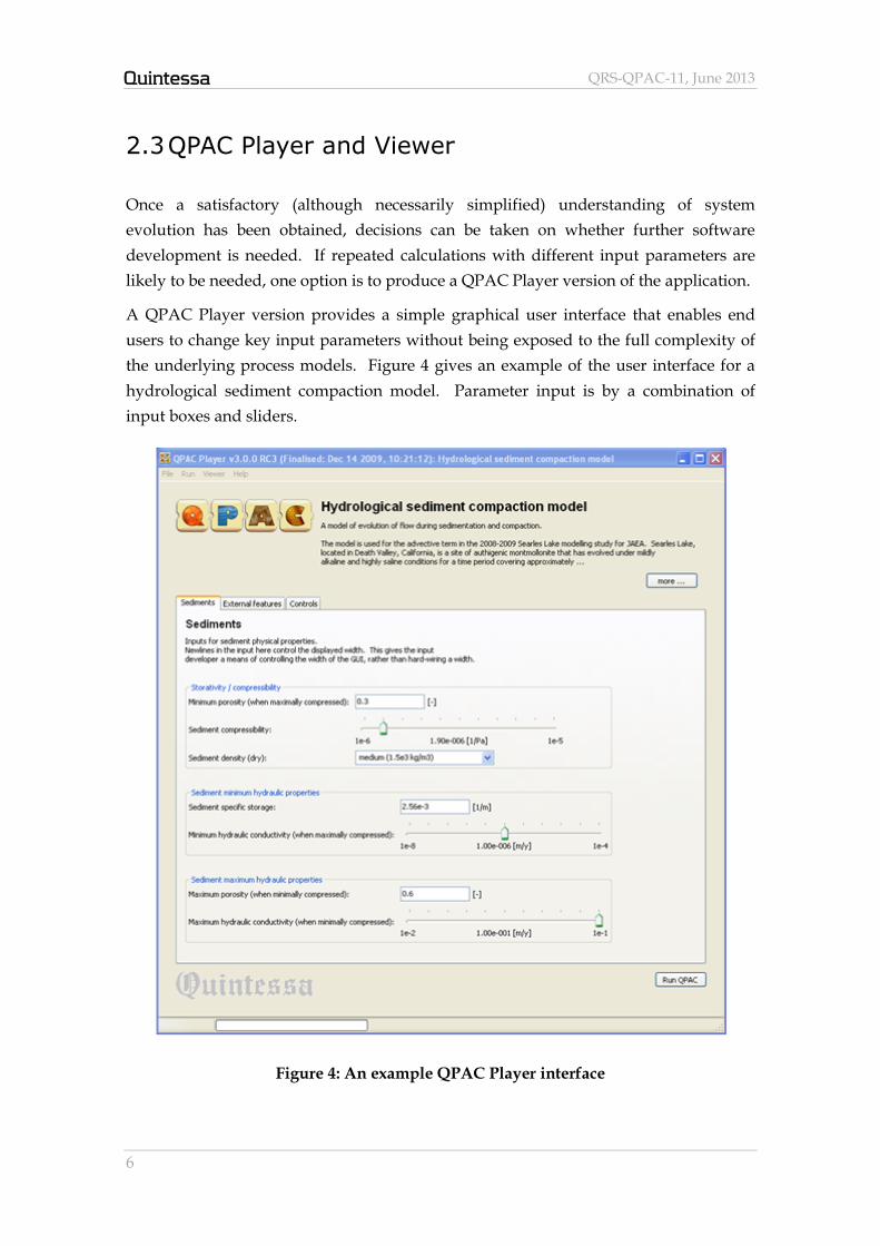
Calculations from a QPAC Player application are displayed in QPAC Viewer. This tool

is designed to help the modeller visualise their model in 3D, navigate easily between

subsystems and view model output quickly. Tools are provided for zooming, panning

and rotating so that the modeller can inspect all parts of their model. An example of

the Viewer interface is shown in Figure 5.

Figure 5: QPAC Viewer interface

QPAC Viewer allows the modeller to select any of the outputs and show the values

using colour coding. Output times can be cycled through automatically, effectively

generating a ‘movie’ so that the modeller can view the evolution of the system.

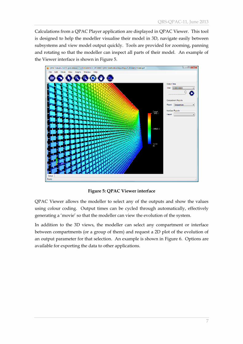
In addition to the 3D views, the modeller can select any compartment or interface

between compartments (or a group of them) and request a 2D plot of the evolution of

an output parameter for that selection. An example is shown in Figure 6. Options are

available for exporting the data to other applications.


8

Figure 6: An Evolution Plot provided by QPAC Viewer


9

3 Carbon Dioxide in the Terrestrial Environment

Carbon dioxide (CO2) is the most important greenhouse gas and carbon capture and

storage (CCS) is one of the technologies being considered to reduce the release of this

gas to the atmosphere. CCS involves compressing the gas and pumping it into deep

geological strata, generally in a supercritical state. QPAC has been employed in a

number of different studies concerned with the behaviour of CO2 in terrestrial

environments and some examples are given in this section.

3.1 A Site with Naturally High CO2 Surface Fluxes

Understanding the behaviour of CO2 in areas with naturally-occurring high surface

fluxes of CO2 can provide valuable information for CO2 storage technology. If the key

processes taking place at such sites can be satisfactorily understood with the aid of

systems models and supporting detailed models for particular parts of the system, this

gives confidence in the application of the models to engineered sites. Here some details

are given of the modelling that has been undertaken for the Latera site in Italy; more

details, including the references to the data that were employed, are given in Maul et

al. (2009).

A conceptual model for CO2 transport at the site was produced with the system

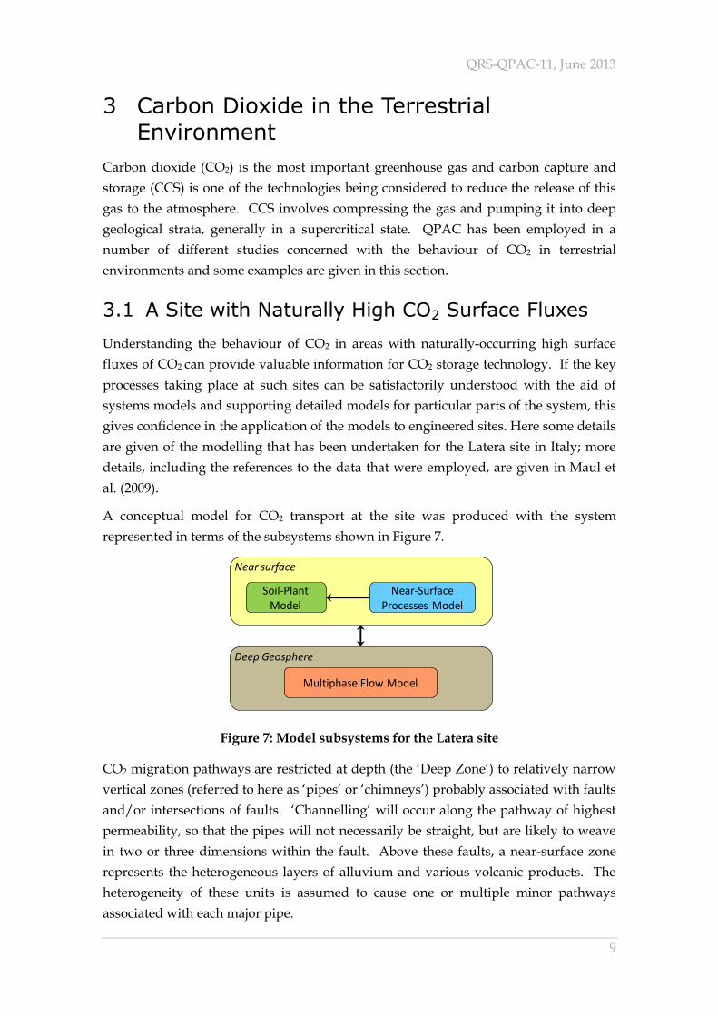
represented in terms of the subsystems shown in Figure 7.

Figure 7: Model subsystems for the Latera site

CO2 migration pathways are restricted at depth (the ‘Deep Zone’) to relatively narrow

vertical zones (referred to here as ‘pipes’ or ‘chimneys’) probably associated with faults

and/or intersections of faults. ‘Channelling’ will occur along the pathway of highest

permeability, so that the pipes will not necessarily be straight, but are likely to weave

in two or three dimensions within the fault. Above these faults, a near-surface zone

represents the heterogeneous layers of alluvium and various volcanic products. The

heterogeneity of these units is assumed to cause one or multiple minor pathways

associated with each major pipe.

Multiphase Flow Model

Near surface

Deep Geosphere

Soil-Plant Model

Near-Surface Processes Model


10

The deep geosphere part of the system was modelled very simply, with a specified CO2

production rate at depth and transport vertically to the near-surface environment

through one or more stochastically generated pipes, each representing an open fault

intersection in the bedrock connected to the common carbonate ‘reservoir’ of CO2.

The near-surface processes subsystem represents processes that are relevant to the

transport of CO2 immediately below the water table and between the water table and

the surface.

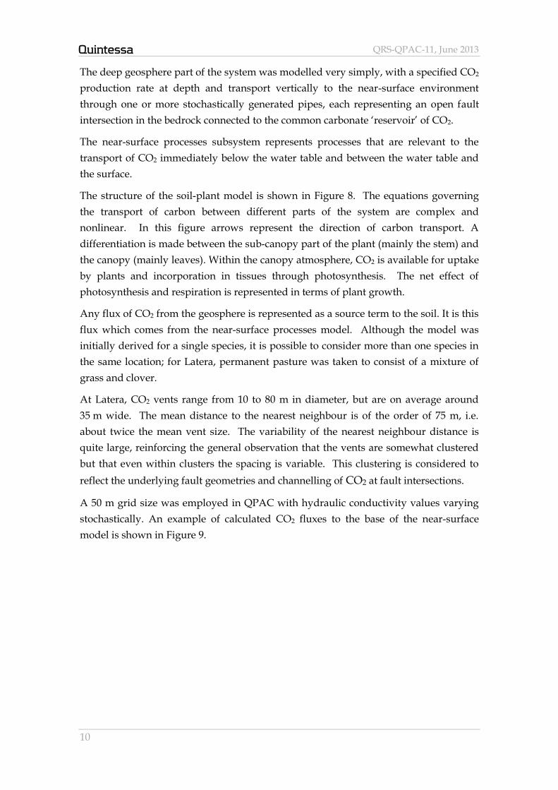
The structure of the soil-plant model is shown in Figure 8. The equations governing

the transport of carbon between different parts of the system are complex and

nonlinear. In this figure arrows represent the direction of carbon transport. A

differentiation is made between the sub-canopy part of the plant (mainly the stem) and

the canopy (mainly leaves). Within the canopy atmosphere, CO2 is available for uptake

by plants and incorporation in tissues through photosynthesis. The net effect of

photosynthesis and respiration is represented in terms of plant growth.

Any flux of CO2 from the geosphere is represented as a source term to the soil. It is this

flux which comes from the near-surface processes model. Although the model was

initially derived for a single species, it is possible to consider more than one species in

the same location; for Latera, permanent pasture was taken to consist of a mixture of

grass and clover.

At Latera, CO2 vents range from 10 to 80 m in diameter, but are on average around

35 m wide. The mean distance to the nearest neighbour is of the order of 75 m, i.e.

about twice the mean vent size. The variability of the nearest neighbour distance is

quite large, reinforcing the general observation that the vents are somewhat clustered

but that even within clusters the spacing is variable. This clustering is considered to

reflect the underlying fault geometries and channelling of CO2 at fault intersections.

A 50 m grid size was employed in QPAC with hydraulic conductivity values varying

stochastically. An example of calculated CO2 fluxes to the base of the near-surface

model is shown in Figure 9.


11

Figure 8: Structure of the soil-plant model

Figure 9: Plan view of calculated fluxes of CO2 (kg CO2 m-2 d-1) to the surface at equilibrium (shown as equivalent flux density through surface vents)


12

A cluster of surface vents is created for each input from a deep pipe. The calculated

carbon fluxes at the higher end of the spectrum cluster around approximately

70 kg C m-2 y-1, which corresponds to approximately 0.7 kg CO2 m-2 d-1; this is

consistent with the typical mean fluxes across vents that cause substantial plant loss

(typically in the range 0.2 to 1.8 kg CO2 m-2 d-1). The pattern of CO2 venting calculated

is broadly consistent with field observations at the site.

During field campaigns in September 2005 and June 2006, data were collected for a

single vent and the soil-plant model was used to simulate conditions at three locations.

Although it was not possible to make detailed comparisons between measurements

and model calculations, overall the soil-plant model represented the key features

observed. The calculated CO2 concentrations in the rooting zone were comparable with

measured values at a depth of 20 cm, and the modelled biomass was comparable with

the estimated biomass values from the empirical data.

The models used at the Latera site are currently being developed for application to

both natural sites and field experiments in the UK and Norway in an EU-funded

research programme, RISCS (www.riscs-co2.eu).

3.2 Systems Modelling of Terrestrial Storage Sites

QPAC has been used in a number of performance assessments of actual and potential

sites for the geological storage of CO2. QPAC calculations can be used to complement

calculations of CO2 transport undertaken using dedicated codes. In general QPAC will

use a coarser discretisation of the system than dedicated reservoir simulators, but it is

easier to add different processes in order to undertake sensitivity studies and to

address ‘what if’ questions about how the CO2 might migrate over long timescales.

Figure 10 compares spatial variations in post-closure CO2 saturation in a deep

sedimentary rock reservoir considered by Metcalfe et al. (2009), as simulated by a

finely discretised reservoir code and a simplified, coarsely discretised QPAC model.

Expert evaluation of information about the reservoir suggested that undetected fluid

flow pathways might occur through the caprock (the geological stratum above the host

stratum containing the CO2). Sensitivity studies using the QPAC model investigated

the potential significance of leakage through these possible features, as shown in

Figure 11. The model used for these studies was parameterised using a combination of

site observations and expert judgments based upon them. These calculations can be

used to provide input to decisions on the overall performance of the storage system.

http://www.riscs-co2.eu/


13

Figure 10: A finely discretised reservoir model (left) and a simplified, coarsely discretised QPAC model (right). The two sets of model output are mirror images.

Figure 11: QPAC calculations to evaluate the potential significance of leakage through undetected features in the caprock

QPAC model

Course discretization:

600 compartments

1500 interfaces

Standard reservoir model

Fine discretization:

50,000 cells

0 km

8 km

6 km

0% CO2

100% CO2

0 km

-1 km

0 100 200 300 400 500 600 700 800 900 1000

Time, years

Rel

ease

d f

ract

ion

of

store

d C

O2 0.035

0.03

0.025

0.02

0.015

0.01

0.005

0.0

BaseShorter

spill length

Lower shale

resistance

Potential leakages through undetected

features

Increased sand

permeability

Criterion:

<2% in

1000 years


14

3.3 Detailed Modelling of Cement Well Seals

Important features of geological storage systems for CO2 are cement well seals. This is

an example of where QPAC has been employed to undertake fully-coupled

geochemical modelling, focusing on cement degradation. Details of work that has been

undertaken in this area, and the data that have been employed, are given in Wilson et

al. (2011); a brief summary is given here.

The QPAC models were developed using the reactive transport module. The aim was

to represent the relevant chemical processes as simply as possible, in order to

reproduce key features of data from experiments and field observations. Figure 12

gives an example of the QPAC calculations for the chemical evolution of the well seal,

showing the calculated volume fractions of the different phases over a 100 year period.

It was found that reasonable agreement with the limited field data over 30 years was

obtained, provided the Pitzer approach (Pitzer, 1987) was employed for the

thermodynamic modelling of solutions; this approach is more appropriate than other

commonly-used methods when modelling high concentration saline fluids. This helps

provide confidence in the calculations over longer periods, although many

uncertainties remain and this continues to be an area of active research.

Figure 12: Volume fraction plots of solid phases for 30 and 100 year QPAC simulations of the SACROC field data (Carey et al., 2007)

3.4 Detailed Modelling of Two-Phase Flow

When supercritical CO2 is injected through an injection well the resulting two-phase

flow in heterogeneous geology is complex. When considering coupled process

modelling the location of the interface is of importance as most interactions occur

there. McDermott et al. (2011) compared different methods for undertaking such

calculations. QPAC calculations (using the finite volume approach) were compared

with a hybrid method that uses finite elements combined with analytical techniques.

Figure 13 shows an example QPAC calculation which used the multiphase flow (MPF)

module, illustrating the effects of the heterogeneous conditions. Although there were


15

detailed differences between these calculations and those obtained from dedicated

models, the QPAC calculations reproduced the key features of the system evolution, in

particular the location of the CO2 front.

Figure 13: QPAC calculations of the injection of supercritical CO2 into a heterogeneous reservoir rock


16

4 Geochemical Modelling

QPAC has been applied to a number of complex geochemical problems and some

examples that illustrate this capability are given in this section. All of these examples

use the reactive transport module, which allows simulations to be undertaken for

interactions between subsurface fluids, rocks and engineered structures. The reactive

transport equations fully couple the fluid flow equations with those representing

geochemical reactions between porewater components and solid materials.

Reactive transport calculations are technically challenging. ‘Dedicated’ codes can often

fail to solve some problems, for example when geochemical reactions result in porosity

becoming ‘clogged’. The flexible approach that is possible with QPAC means that

models can be adapted as necessary, for example to use:

different mathematical formulations;

different conceptual models (sometimes the physics is wrong...);

different smoothing strategies (space/time dependent); or

different couplings (e.g. imposing limits on the abundance of key ions in a

reaction).

These capabilities often allow progress to be made using QPAC when this cannot be

done with other codes. Two examples of the use of QPAC in this area are summarised

here. The use of QPAC for long-term modelling of cements is described in Savage et

al. (2011).

4.1 A Natural Clay System in Alkaline Conditions

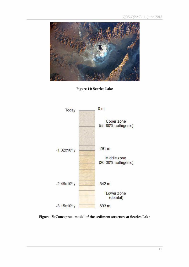
Searles Lake (Figure 14) is a dry lake basin near Death Valley in the USA which has

provided useful information on the long-term evolution of bentonite clay (an

important component in many design concepts for geological disposal facilities for

radioactive waste). The timescale involved (around three million years) is beyond that

which can be considered in laboratory experiments.

QPAC has been used to describe the evolution of this system (Savage et al., 2010a).

The conceptual model for the structure of the sediments is shown in Figure 15.

Sediments are laid down at a rate of around 22 cm in a thousand years. The

composition of the infiltrating water has changed with time (giving a time-dependent

boundary condition) so that different sediments experience a different pore water

history. This results in varying sediment alteration with time and depth with deeper

sediments becoming compacted with the weight of those above.


17

Figure 14: Searles Lake

Figure 15: Conceptual model of the sediment structure at Searles Lake


18

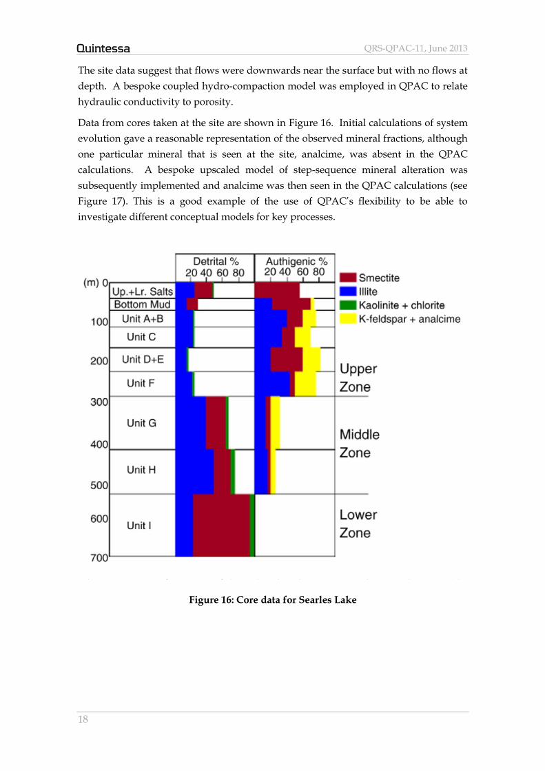
The site data suggest that flows were downwards near the surface but with no flows at

depth. A bespoke coupled hydro-compaction model was employed in QPAC to relate

hydraulic conductivity to porosity.

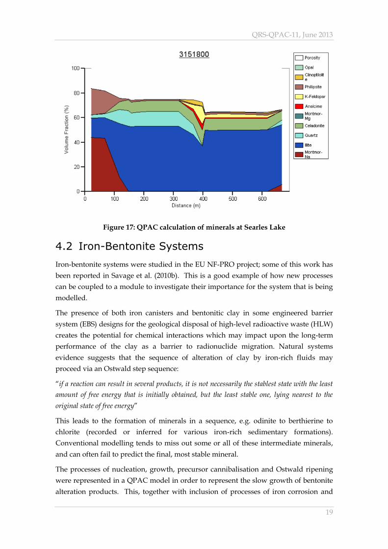
Data from cores taken at the site are shown in Figure 16. Initial calculations of system

evolution gave a reasonable representation of the observed mineral fractions, although

one particular mineral that is seen at the site, analcime, was absent in the QPAC

calculations. A bespoke upscaled model of step-sequence mineral alteration was

subsequently implemented and analcime was then seen in the QPAC calculations (see

Figure 17). This is a good example of the use of QPAC’s flexibility to be able to

investigate different conceptual models for key processes.

Figure 16: Core data for Searles Lake


19

Figure 17: QPAC calculation of minerals at Searles Lake

4.2 Iron-Bentonite Systems

Iron-bentonite systems were studied in the EU NF-PRO project; some of this work has

been reported in Savage et al. (2010b). This is a good example of how new processes

can be coupled to a module to investigate their importance for the system that is being

modelled.

The presence of both iron canisters and bentonitic clay in some engineered barrier

system (EBS) designs for the geological disposal of high-level radioactive waste (HLW)

creates the potential for chemical interactions which may impact upon the long-term

performance of the clay as a barrier to radionuclide migration. Natural systems

evidence suggests that the sequence of alteration of clay by iron-rich fluids may

proceed via an Ostwald step sequence:

“if a reaction can result in several products, it is not necessarily the stablest state with the least

amount of free energy that is initially obtained, but the least stable one, lying nearest to the

original state of free energy”

This leads to the formation of minerals in a sequence, e.g. odinite to berthierine to

chlorite (recorded or inferred for various iron-rich sedimentary formations).

Conventional modelling tends to miss out some or all of these intermediate minerals,

and can often fail to predict the final, most stable mineral.

The processes of nucleation, growth, precursor cannibalisation and Ostwald ripening

were represented in a QPAC model in order to represent the slow growth of bentonite

alteration products. This, together with inclusion of processes of iron corrosion and


20

diffusion, enabled investigation of a representative model of the alteration of bentonite

in a typical EBS environment.

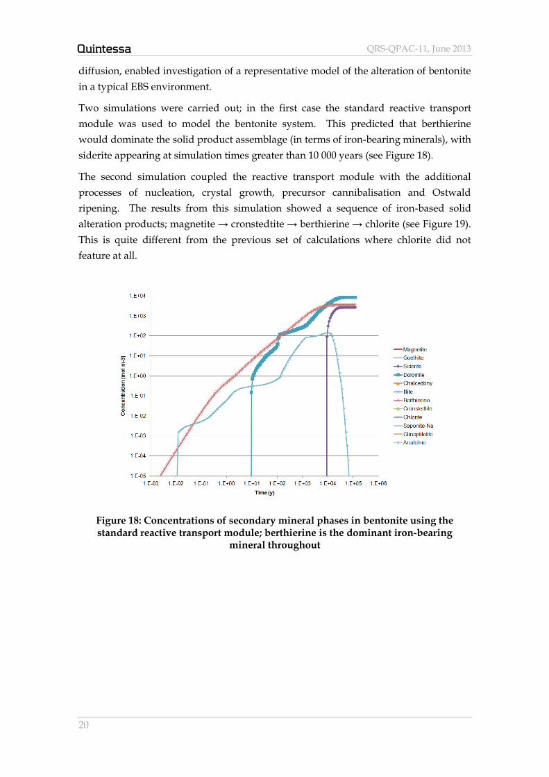
Two simulations were carried out; in the first case the standard reactive transport

module was used to model the bentonite system. This predicted that berthierine

would dominate the solid product assemblage (in terms of iron-bearing minerals), with

siderite appearing at simulation times greater than 10 000 years (see Figure 18).

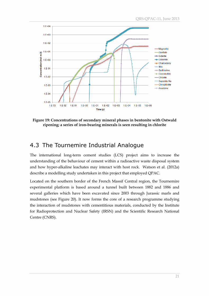
The second simulation coupled the reactive transport module with the additional

processes of nucleation, crystal growth, precursor cannibalisation and Ostwald

ripening. The results from this simulation showed a sequence of iron-based solid

alteration products; magnetite → cronstedtite → berthierine → chlorite (see Figure 19).

This is quite different from the previous set of calculations where chlorite did not

feature at all.

Figure 18: Concentrations of secondary mineral phases in bentonite using the standard reactive transport module; berthierine is the dominant iron-bearing

mineral throughout


21

Figure 19: Concentrations of secondary mineral phases in bentonite with Ostwald ripening; a series of iron-bearing minerals is seen resulting in chlorite

4.3 The Tournemire Industrial Analogue

The international long-term cement studies (LCS) project aims to increase the

understanding of the behaviour of cement within a radioactive waste disposal system

and how hyper-alkaline leachates may interact with host rock. Watson et al. (2012a)

describe a modelling study undertaken in this project that employed QPAC.

Located on the southern border of the French Massif Central region, the Tournemire

experimental platform is based around a tunnel built between 1882 and 1886 and

several galleries which have been excavated since 2003 through Jurassic marls and

mudstones (see Figure 20). It now forms the core of a research programme studying

the interaction of mudstones with cementitious materials, conducted by the Institute

for Radioprotection and Nuclear Safety (IRSN) and the Scientific Research National

Centre (CNRS).


22

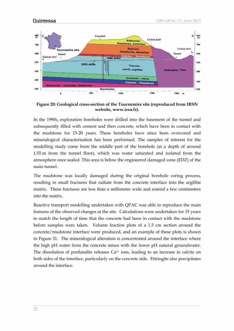
Figure 20: Geological cross-section of the Tournemire site (reproduced from IRSN website, www.irsn.fr).

In the 1990s, exploration boreholes were drilled into the basement of the tunnel and

subsequently filled with cement and then concrete, which have been in contact with

the mudstone for 15-20 years. These boreholes have since been overcored and

mineralogical characterisation has been performed. The samples of interest for the

modelling study come from the middle part of the borehole (at a depth of around

1.55 m from the tunnel floor), which was water saturated and isolated from the

atmosphere once sealed. This area is below the engineered damaged zone (EDZ) of the

main tunnel.

The mudstone was locally damaged during the original borehole coring process,

resulting in small fractures that radiate from the concrete interface into the argillite

matrix. These fractures are less than a millimetre wide and extend a few centimetres

into the matrix.

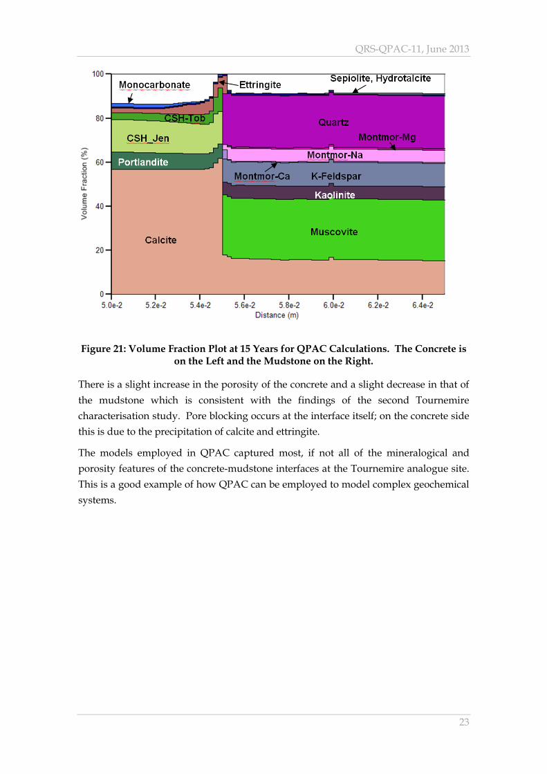
Reactive transport modelling undertaken with QPAC was able to reproduce the main

features of the observed changes at the site. Calculations were undertaken for 15 years

to match the length of time that the concrete had been in contact with the mudstone

before samples were taken. Volume fraction plots of a 1.5 cm section around the

concrete/mudstone interface were produced, and an example of these plots is shown

in Figure 21. The mineralogical alteration is concentrated around the interface where

the high pH water from the concrete mixes with the lower pH natural groundwater.

The dissolution of portlandite releases Ca2+ ions, leading to an increase in calcite on

both sides of the interface, particularly on the concrete side. Ettringite also precipitates

around the interface.


23

Figure 21: Volume Fraction Plot at 15 Years for QPAC Calculations. The Concrete is on the Left and the Mudstone on the Right.

There is a slight increase in the porosity of the concrete and a slight decrease in that of

the mudstone which is consistent with the findings of the second Tournemire

characterisation study. Pore blocking occurs at the interface itself; on the concrete side

this is due to the precipitation of calcite and ettringite.

The models employed in QPAC captured most, if not all of the mineralogical and

porosity features of the concrete-mudstone interfaces at the Tournemire analogue site.

This is a good example of how QPAC can be employed to model complex geochemical

systems.


24

5 Fluid Flow and Transport

There are a number of commercially available, dedicated software tools for

undertaking flow and transport calculations. The QPAC multiphase flow (MPF)

modules do not provide all the features of such tools, but the ability to modify process

representations with QPAC can be valuable when undertaking sensitivity calculations

or when investigating conceptual model uncertainty; two examples of QPAC

calculations in this area are summarised here.

5.1 Repository Resaturation Calculations

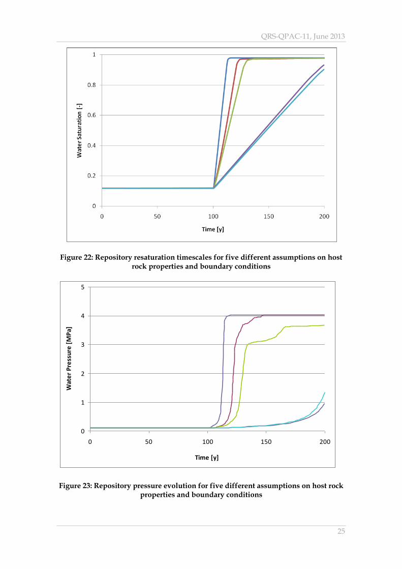
Independent calculations were undertaken for SKI, the Swedish nuclear power

regulator (now part of the Swedish Radiation Safety Authority, SSM) as input to their

review of the SR-Can performance assessment for a deep radioactive waste repository

in Sweden (Maul et al., 2008). In this repository design deposition holes are to be made

in crystalline rock with large metal canisters containing the spent nuclear fuel and a

bentonite clay buffer between the canister and the rock.

The saturation of the repository was simulated using QPAC. The calculations enable

conclusions to be drawn about the sensitivity of resaturation times after repository

closure to various assumptions about the system behaviour; the way that the

repository resaturates is important for the evolution of the engineered barrier systems.

Figure 22 and Figure 23 show example calculations of the evolution with time of the

saturation and pressure in the repository for five different assumptions about the rock

permeabilities and boundary conditions. Upon excavation and desaturation of the

repository, water pressures drop, as do water saturations. The drop in water

saturation is a reflection of the fact that the inflow at the top boundary is insufficient to

maintain full water saturation under these vertical water head gradients.

Another example of the use of QPAC to undertake repository resaturation calculations

is described by Bond et al. (2009).


25

Figure 22: Repository resaturation timescales for five different assumptions on host rock properties and boundary conditions

Figure 23: Repository pressure evolution for five different assumptions on host rock properties and boundary conditions

0

1

2

3

4

5

0 50 100 150 200

Time [y]

Wat

er

Pre

ssu

re [

MP

a]


26

5.2 Gas Flow in Disposal Facilities and the FORGE

Project

FORGE is an EU project that considered research issues associated with the generation,

fate and transport of gases generated in radioactive waste disposal facilities

(www.bgs.ac.uk/forge/). In this project Quintessa provided technical support to the

UK Nuclear Decommissioning Authority (NDA) for Work Package 1 (Treatment of Gas

in Performance Assessment). This work package focussed on the complex issue of

understanding how to characterise and represent gas migration in manner suitable to

support whole facility performance assessments.

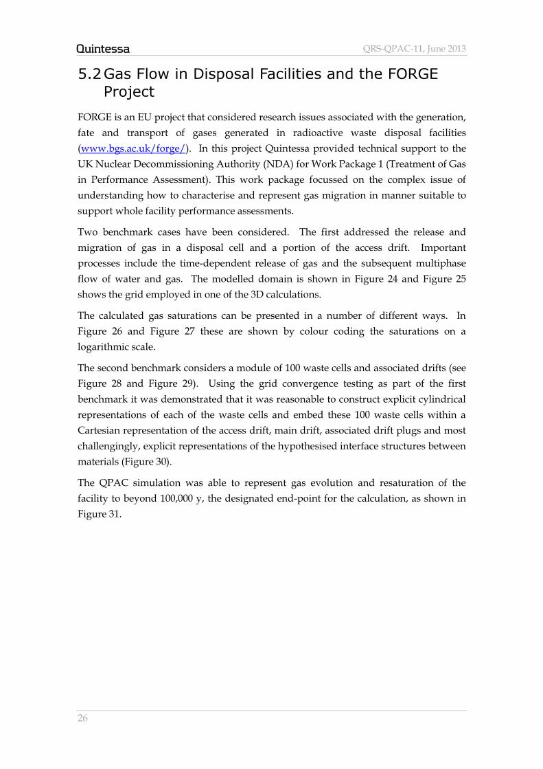
Two benchmark cases have been considered. The first addressed the release and

migration of gas in a disposal cell and a portion of the access drift. Important

processes include the time-dependent release of gas and the subsequent multiphase

flow of water and gas. The modelled domain is shown in Figure 24 and Figure 25

shows the grid employed in one of the 3D calculations.

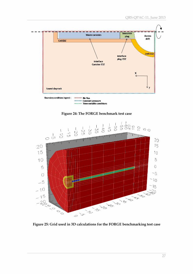
The calculated gas saturations can be presented in a number of different ways. In

Figure 26 and Figure 27 these are shown by colour coding the saturations on a

logarithmic scale.

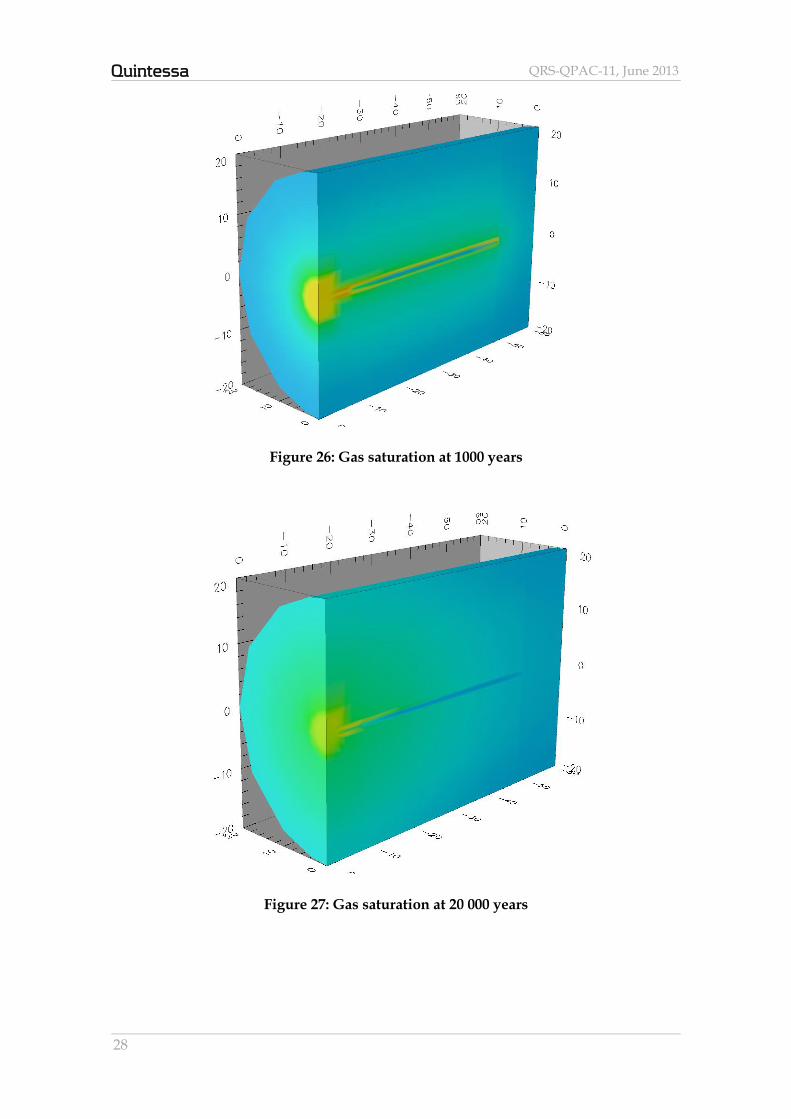
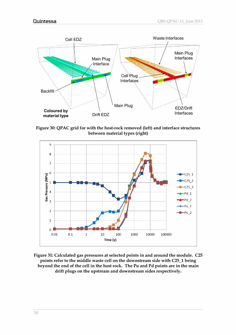
The second benchmark considers a module of 100 waste cells and associated drifts (see

Figure 28 and Figure 29). Using the grid convergence testing as part of the first

benchmark it was demonstrated that it was reasonable to construct explicit cylindrical

representations of each of the waste cells and embed these 100 waste cells within a

Cartesian representation of the access drift, main drift, associated drift plugs and most

challengingly, explicit representations of the hypothesised interface structures between

materials (Figure 30).

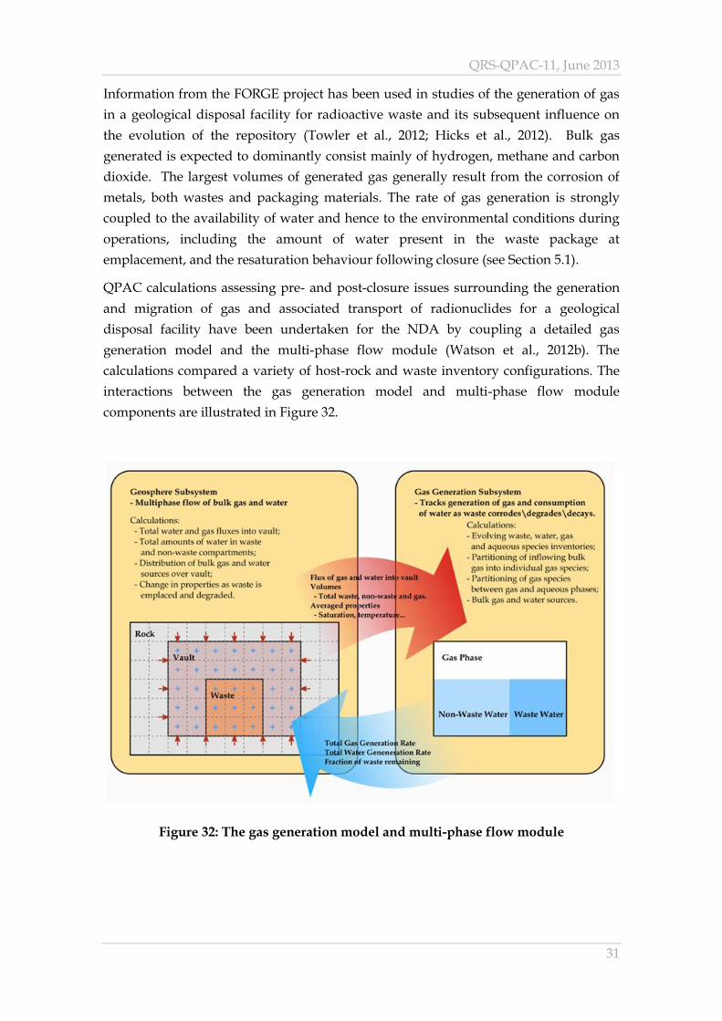
The QPAC simulation was able to represent gas evolution and resaturation of the

facility to beyond 100,000 y, the designated end-point for the calculation, as shown in

Figure 31.

http://www.bgs.ac.uk/forge/


27

Figure 24: The FORGE benchmark test case

Figure 25: Grid used in 3D calculations for the FORGE benchmarking test case


28

Figure 26: Gas saturation at 1000 years

Figure 27: Gas saturation at 20 000 years


29

Figure 28: Vertical section through the module for the second benchmark

Figure 29: Plan view of the geometry for the second benchmark


30

Figure 30: QPAC grid for with the host-rock removed (left) and interface structures between material types (right)

Figure 31: Calculated gas pressures at selected points in and around the module. C25 points refer to the middle waste cell on the downstream side with C25_1 being

beyond the end of the cell in the host rock. The Pu and Pd points are in the main drift plugs on the upstream and downstream sides respectively.


31

Information from the FORGE project has been used in studies of the generation of gas

in a geological disposal facility for radioactive waste and its subsequent influence on

the evolution of the repository (Towler et al., 2012; Hicks et al., 2012). Bulk gas

generated is expected to dominantly consist mainly of hydrogen, methane and carbon

dioxide. The largest volumes of generated gas generally result from the corrosion of

metals, both wastes and packaging materials. The rate of gas generation is strongly

coupled to the availability of water and hence to the environmental conditions during

operations, including the amount of water present in the waste package at

emplacement, and the resaturation behaviour following closure (see Section 5.1).

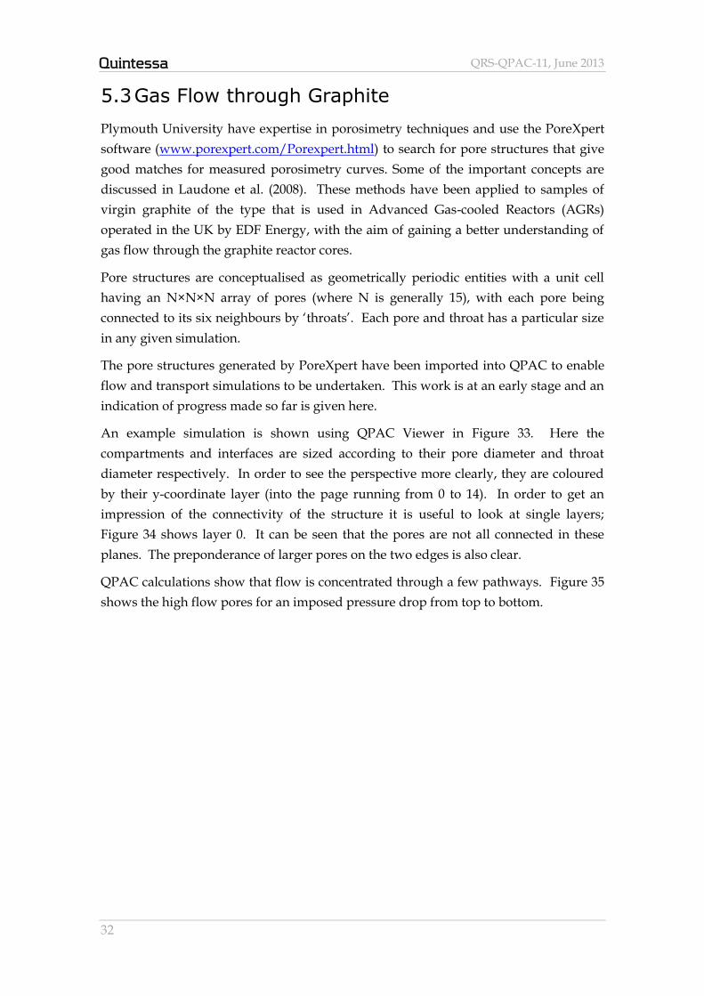
QPAC calculations assessing pre- and post-closure issues surrounding the generation

and migration of gas and associated transport of radionuclides for a geological

disposal facility have been undertaken for the NDA by coupling a detailed gas

generation model and the multi-phase flow module (Watson et al., 2012b). The

calculations compared a variety of host-rock and waste inventory configurations. The

interactions between the gas generation model and multi-phase flow module

components are illustrated in Figure 32.

Figure 32: The gas generation model and multi-phase flow module


32

5.3 Gas Flow through Graphite

Plymouth University have expertise in porosimetry techniques and use the PoreXpert

software (www.porexpert.com/Porexpert.html) to search for pore structures that give

good matches for measured porosimetry curves. Some of the important concepts are

discussed in Laudone et al. (2008). These methods have been applied to samples of

virgin graphite of the type that is used in Advanced Gas-cooled Reactors (AGRs)

operated in the UK by EDF Energy, with the aim of gaining a better understanding of

gas flow through the graphite reactor cores.

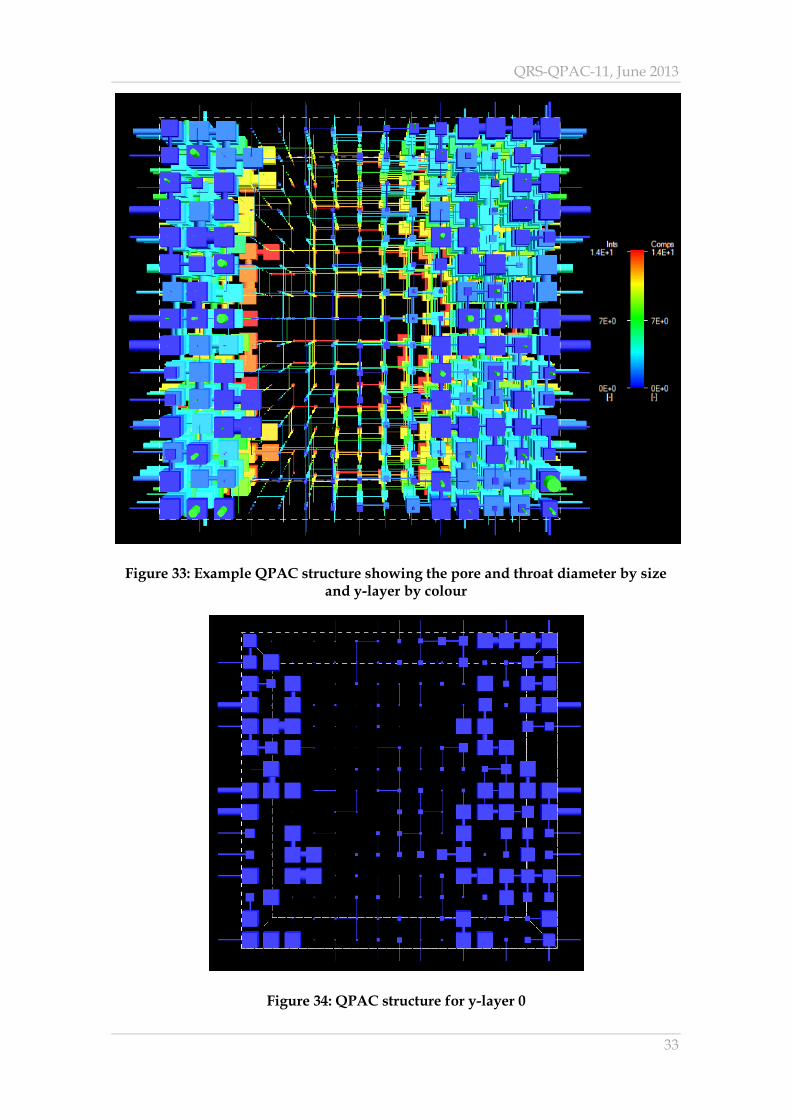
Pore structures are conceptualised as geometrically periodic entities with a unit cell

having an N×N×N array of pores (where N is generally 15), with each pore being

connected to its six neighbours by ‘throats’. Each pore and throat has a particular size

in any given simulation.

The pore structures generated by PoreXpert have been imported into QPAC to enable

flow and transport simulations to be undertaken. This work is at an early stage and an

indication of progress made so far is given here.

An example simulation is shown using QPAC Viewer in Figure 33. Here the

compartments and interfaces are sized according to their pore diameter and throat

diameter respectively. In order to see the perspective more clearly, they are coloured

by their y-coordinate layer (into the page running from 0 to 14). In order to get an

impression of the connectivity of the structure it is useful to look at single layers;

Figure 34 shows layer 0. It can be seen that the pores are not all connected in these

planes. The preponderance of larger pores on the two edges is also clear.

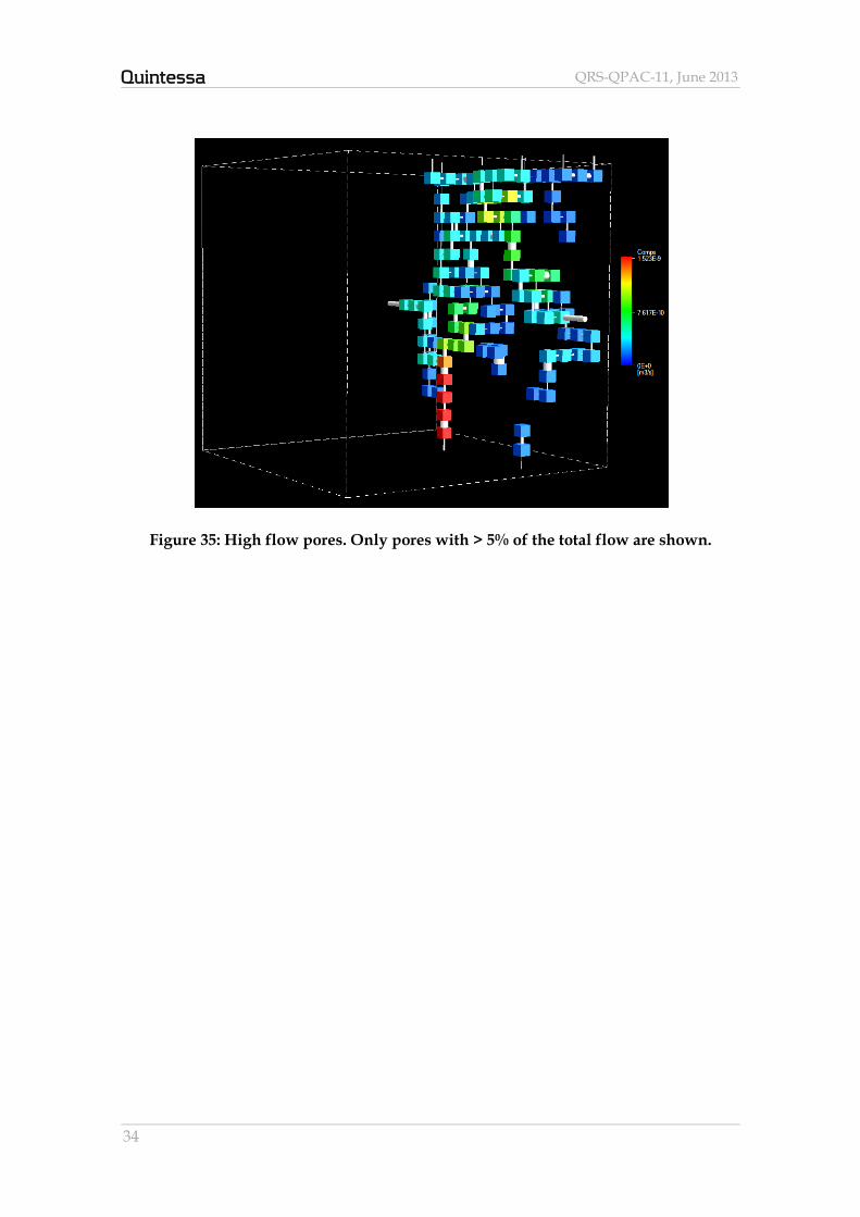
QPAC calculations show that flow is concentrated through a few pathways. Figure 35

shows the high flow pores for an imposed pressure drop from top to bottom.

http://www.porexpert.com/Porexpert.html


33

Figure 33: Example QPAC structure showing the pore and throat diameter by size and y-layer by colour

Figure 34: QPAC structure for y-layer 0


34

Figure 35: High flow pores. Only pores with > 5% of the total flow are shown.


35

6 THMC Modelling

QPAC is ideally suited to undertaking problems where coupled Thermal (T),

Hydraulic (H), Mechanical (M) and Chemical (C) processes have to be considered. For

some problems not all types of process will need to be modelled. In this Section some

examples are presented where mechanical processes are important.

6.1 The THERESA Project

Quintessa participated in the EU THERESA project with support from the Swedish

Radiation Safety Authority (SSM). This project aimed to develop the capabilities of

mathematical models and computer codes applied to the design, construction,

operation, performance and safety assessment, and post-closure monitoring of

geological nuclear waste repositories, based on the scientific principles governing

coupled thermo-hydro-mechanical and chemical (THMC) processes in geological

systems. The project was completed at the end of 2009. Comparisons were made

between QPAC calculations and benchmarking test cases. Brief examples of these

comparisons are given here; more details are given in Maul et al. (2010).

6.1.1 Benchmarking Test Cases

Three test cases were undertaken, each of which involved the calculation of relatively

small (cm to m scale) bentonite evolution under resaturation conditions. The three

cases each examined different configurations of available external water (Case 3 having

no external inflow of water), mechanical confinement, applied heat and bentonite

properties.

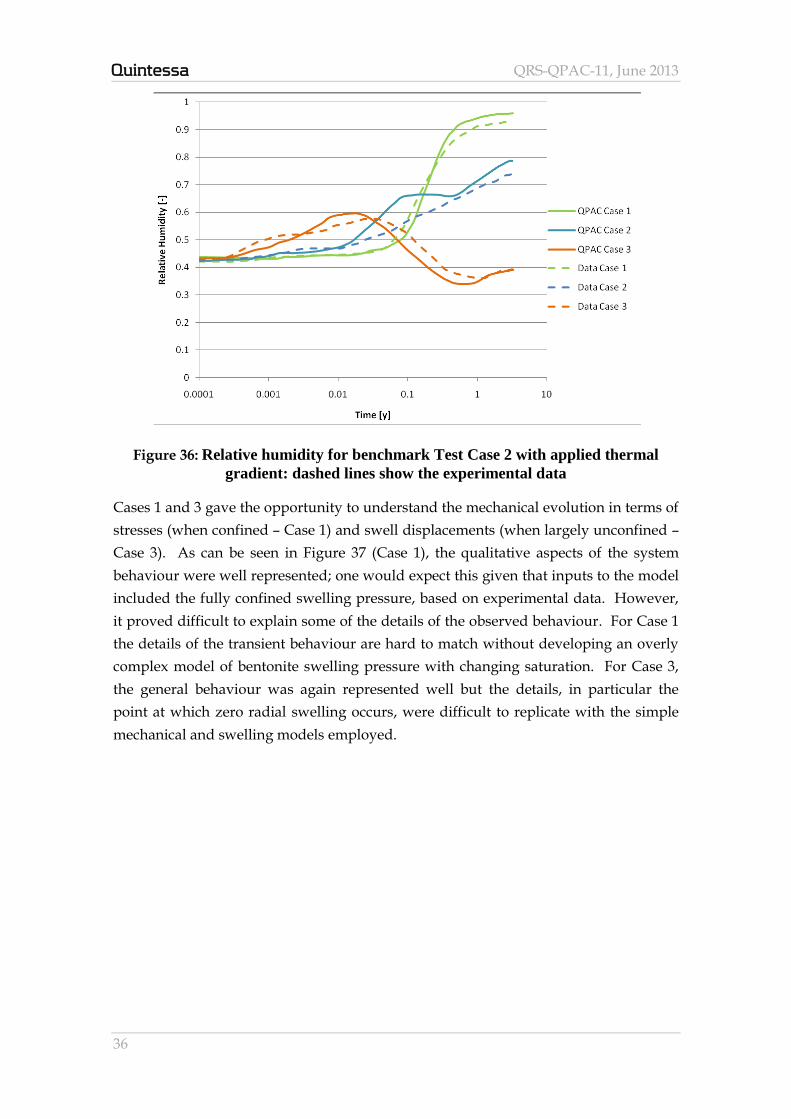
The understanding of hydraulic evolution was largely through measured relative

humidities (Case 1 and 2), the total amount of water entering the system (Case 1 and 2)

and the measured water content at the end of the experiment (Case 1 and 3). In all

cases a good qualitative and quantitative match to the observed data was obtained

using a broadly consistent set of parameters and hydraulic models for relative

humidity and water content. Illustrative calculations are shown in Figure 36.


36

Figure 36: Relative humidity for benchmark Test Case 2 with applied thermal

gradient: dashed lines show the experimental data

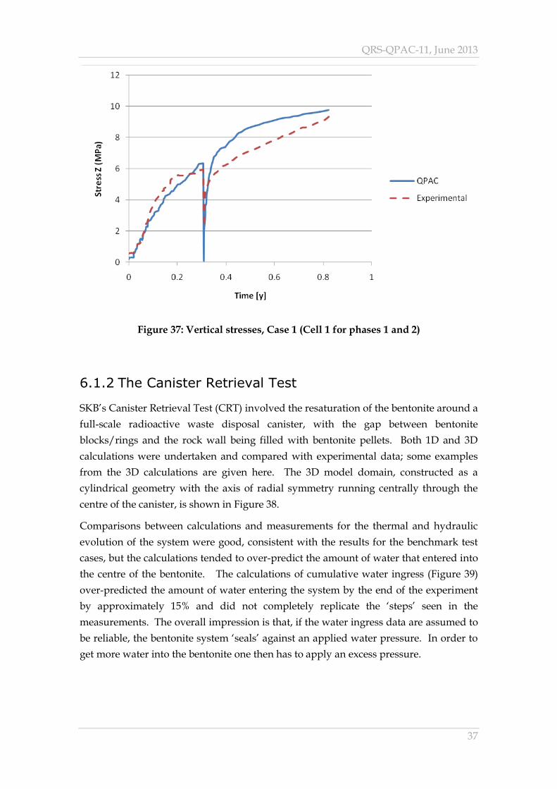
Cases 1 and 3 gave the opportunity to understand the mechanical evolution in terms of

stresses (when confined – Case 1) and swell displacements (when largely unconfined –

Case 3). As can be seen in Figure 37 (Case 1), the qualitative aspects of the system

behaviour were well represented; one would expect this given that inputs to the model

included the fully confined swelling pressure, based on experimental data. However,

it proved difficult to explain some of the details of the observed behaviour. For Case 1

the details of the transient behaviour are hard to match without developing an overly

complex model of bentonite swelling pressure with changing saturation. For Case 3,

the general behaviour was again represented well but the details, in particular the

point at which zero radial swelling occurs, were difficult to replicate with the simple

mechanical and swelling models employed.


37

Figure 37: Vertical stresses, Case 1 (Cell 1 for phases 1 and 2)

6.1.2 The Canister Retrieval Test

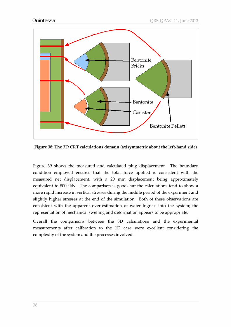
SKB’s Canister Retrieval Test (CRT) involved the resaturation of the bentonite around a

full-scale radioactive waste disposal canister, with the gap between bentonite

blocks/rings and the rock wall being filled with bentonite pellets. Both 1D and 3D

calculations were undertaken and compared with experimental data; some examples

from the 3D calculations are given here. The 3D model domain, constructed as a

cylindrical geometry with the axis of radial symmetry running centrally through the

centre of the canister, is shown in Figure 38.

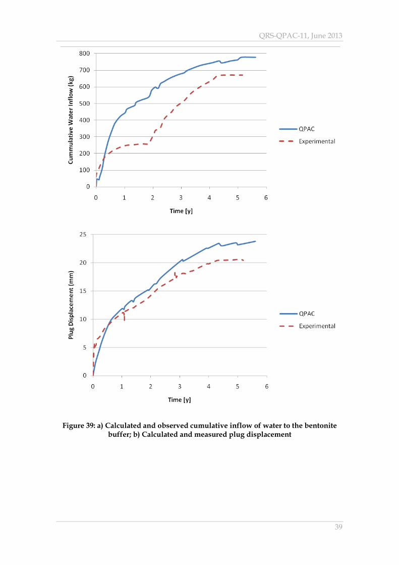
Comparisons between calculations and measurements for the thermal and hydraulic

evolution of the system were good, consistent with the results for the benchmark test

cases, but the calculations tended to over-predict the amount of water that entered into

the centre of the bentonite. The calculations of cumulative water ingress (Figure 39)

over-predicted the amount of water entering the system by the end of the experiment

by approximately 15% and did not completely replicate the ‘steps’ seen in the

measurements. The overall impression is that, if the water ingress data are assumed to

be reliable, the bentonite system ‘seals’ against an applied water pressure. In order to

get more water into the bentonite one then has to apply an excess pressure.


38

Figure 38: The 3D CRT calculations domain (axisymmetric about the left-hand side)

Figure 39 shows the measured and calculated plug displacement. The boundary

condition employed ensures that the total force applied is consistent with the

measured net displacement, with a 20 mm displacement being approximately

equivalent to 8000 kN. The comparison is good, but the calculations tend to show a

more rapid increase in vertical stresses during the middle period of the experiment and

slightly higher stresses at the end of the simulation. Both of these observations are

consistent with the apparent over-estimation of water ingress into the system; the

representation of mechanical swelling and deformation appears to be appropriate.

Overall the comparisons between the 3D calculations and the experimental

measurements after calibration to the 1D case were excellent considering the

complexity of the system and the processes involved.


39

Figure 39: a) Calculated and observed cumulative inflow of water to the bentonite buffer; b) Calculated and measured plug displacement


40

6.2 The DECOVALEX Project

Quintessa, in conjunction with the University of Edinburgh and the Centre for

Environmental Research, UFZ Leipzig, participated in the DECOVALEX-2011 project,

in support of the Nuclear Decommissioning Authority Radioactive Waste Management

Directorate (NDA RWMD). This work builds on previous DECOVALEX projects (see,

for example, Tsang et al., 2005) aimed at improving understanding of THMC

processes, through developing numerical models in comparison with laboratory and

field data and using this understanding to improve performance and safety

assessments for radioactive waste repositories.

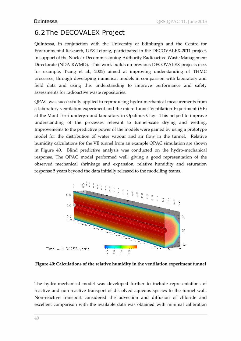
QPAC was successfully applied to reproducing hydro-mechanical measurements from

a laboratory ventilation experiment and the micro-tunnel Ventilation Experiment (VE)

at the Mont Terri underground laboratory in Opalinus Clay. This helped to improve

understanding of the processes relevant to tunnel-scale drying and wetting.

Improvements to the predictive power of the models were gained by using a prototype

model for the distribution of water vapour and air flow in the tunnel. Relative

humidity calculations for the VE tunnel from an example QPAC simulation are shown

in Figure 40. Blind predictive analysis was conducted on the hydro-mechanical

response. The QPAC model performed well, giving a good representation of the

observed mechanical shrinkage and expansion, relative humidity and saturation

response 5 years beyond the data initially released to the modelling teams.

Figure 40: Calculations of the relative humidity in the ventilation experiment tunnel

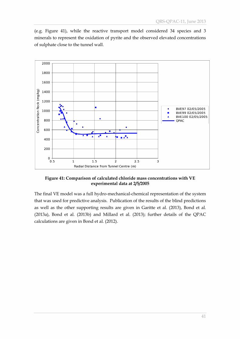
The hydro-mechanical model was developed further to include representations of

reactive and non-reactive transport of dissolved aqueous species to the tunnel wall.

Non-reactive transport considered the advection and diffusion of chloride and

excellent comparison with the available data was obtained with minimal calibration


41

(e.g. Figure 41), while the reactive transport model considered 34 species and 3

minerals to represent the oxidation of pyrite and the observed elevated concentrations

of sulphate close to the tunnel wall.

Figure 41: Comparison of calculated chloride mass concentrations with VE experimental data at 2/5/2005

The final VE model was a full hydro-mechanical-chemical representation of the system

that was used for predictive analysis. Publication of the results of the blind predictions

as well as the other supporting results are given in Garitte et al. (2013), Bond et al.

(2013a), Bond et al. (2013b) and Millard et al. (2013); further details of the QPAC

calculations are given in Bond et al. (2012).


42

References

Bond A E, Norris S, Paulley A and Towler G (2009). Implementation of a Geological

Disposal Facility (GDF) in the UK by the NDA Radioactive Waste Management

Directorate (RWMD): Coupled Modelling of Gas Generation and Multiphase Flow

between the Co-Located ILW/LLW and HLW/SF Components of a GDF. Proceedings

of the 12th International Conference on Environmental Remediation and Radioactive

Waste Management ICEM ‘09/DECOM ’09 October 11-15, 2009, Liverpool, UK.

Bond A E, Benbow S J, Wilson J, McDermott C and English M (2012). Coupled Hydro-

Mechanical-Chemical Process Modelling in Argillaceous Formations for DECOVALEX-

2011. Mineralogical Magazine 76 (8) 3131-3143.

Bond A E, Millard A, Nakama S, Zhang C and Garitte B (2013a). Approaches for

Representing Hydro-mechanical Coupling between Engineered Caverns and

Argillaceous Porous Media at Ventilation Experiments, Mont Terri. Journal of Rock

Mechanics and Geotechnical Engineering 5(2), 85-96.

Bond A E, Benbow S J, Wilson J, Millard A, Nakama S, English E, McDermott C and

Garitte B (2013b). Reactive and Non-reactive Transport Modelling in Partially Water

Saturated Argillaceous Porous Media around the Ventilation Experiment, Mont-Terri.

Journal of Rock Mechanics and Geotechnical Engineering 5, 44-57.

Carey J W, Wigand M, Chipera S J, Wolde G, Pawar S and Lichtner P C (2007). Analysis

and Performance of Oil Well Cement with 30 years of CO2 Exposure from the SACROC

Unit, West Texas, USA. Int. J. Green. Gas Cont. 1, 75-85.

Garitte B, Bond A, Millard A, Zhang C, English M, Nakama S and Gens A (2013).

Analysis of Hydro-mechanical Processes in a Ventilated Tunnel in an Argillaceous

Rock on the Basis of Different Modelling Approaches. Journal of Rock Mechanics and

Geotechnical Engineering 5, 1-17.

Hicks T W, Watson S, Norris S, Towler G, Reedha D, Paulley A, Baldwin T and Bond

A E (2012). Interactions between the Co-Located Intermediate-Level Waste/Low-Level

Waste and High-Level Waste/Spent Fuel Components of a Geological Disposal

Facility. Mineralogical Magazine 76(8) 3475-3482.

Laudone G M, Matthews G P and Gane (2008). Modelling Diffusion from Simulated

Porous Structures. Chemical Engineering Science 63, 1987-1996.

Maul P R, Robinson P C, Bond A E and Benbow S J (2008). Independent Calculations

for the SR-Can Assessment: External Review Contribution in Support of SKI’s and SSI’s

Review of SR-Can. SKI Report 2008-12.


43

Maul P R, Beaubien S E, Bond A E, Limer L M C, Lombardi S, Pearce J, Thorne M C

and West J (2009). Modelling the Fate of Carbon Dioxide in the Near-surface

Environment at the Latera Natural Analogue Site. Energy Procedia 1 1879–1885.

Maul P R, Benbow S J, Bond A E and Robinson P C (2010). Modelling Coupled

Processes in the Evolution of Repository Engineered Barrier Systems using QPAC-EBS.

Swedish Radiation Safety Authority (SSM) Report 2010:25.

McDermott C I, Bond A E, Wang W and Kolditz O (2011). Front Tracking using a

Hybrid Analytical Finite Element Approach for Two-Phase Flow Applied to

Supercritical CO2 Replacing Brine in a Heterogeneous Reservoir and Caprock. Transp.

Porous Med. DOI 10.1007/s11242-011-9799-5.

Millard A, Bond A E, Nakama S, Zhang C, Barnichon J-D and Garitte B. (2012).

Accounting for Anisotropic Effects in the Prediction of the Hydro-mechanical

Response of a Ventilated Tunnel in an Argillaceous Rock. International Journal of Rock

Mechanics and Geotechnical Engineering 5(2), 97-109.

Metcalfe R, Maul P R, Benbow S J, Watson C E, Hodgkinson D P, Paulley A, Limer L,

Walke R C and Savage D (2009). A Unified Approach to Performance Assessment (PA)

of Geological CO2 Storage. Energy Procedia 1, 2503–2510.

Pitzer, K S (1987). Thermodynamic Model for Aqueous Solutions of Liquid-like

Density. In: Thermodynamic Modeling of Geological Materials: Minerals, Fluids and

Melts, Carmichael ISE, Eugster HP, editors. Mineralogical Society of America, Reviews

in Mineralogy 17, 97-142.

Savage D, Benbow S, Watson C, Takase H, Ono K, Oda and, Honda A (2010a).

Natural Systems Evidence for the Alteration of Clay under Alkaline Conditions: an

Example from Searles Lake, California. Applied Clay Science 47, 72–81.

Savage D, Watson C E, Benbow S J and Wilson J (2010b). Modelling Iron-Bentonite

Interactions. Applied Clay Science 47, 91-98.

Savage D, Soler J M, Yamaguchi K, Walker C, Honda A, Inagaki M, Watson C,

Wilson J, Benbow S, Gaus I and Rueedi J (2011). A Comparative Study of the

Modelling of Cement Hydration and Cement-Rock Laboratory Experiments. Applied

Geochemistry 26, 1138-1152.

Towler G, Bond A E, Watson S, Norris S, Suckling P and Benbow S (2012).

Understanding the Behaviour of Gas in a Geological Disposal Facility: Modelling

Coupled Processes and Key Features at Different Scales. Mineralogical Magazine 76(8)

3365-3371.

Tsang C-F, Jing L, Stephansson O and Kautsky F (2005). The DECOVALEX III Project:

A Summary of Activities and Lessons Learned. International Journal of Rock

Mechanics and Mining Sciences 42(5-6), 593-610.


44

Versteeg H and Malalasekra W (2007). An Introduction to Computational Fluid

Dynamics: The Finite Volume Method (2nd Edition). Pearson Education Limited.

Watson C E, Savage D, Wilson J, Walker C and Benbow S J (2012a). The Long-term

Cement Studies Project: the UK Contribution to Model Development and Testing.

Mineralogical Magazine 76(8), 3445-3455.

Watson S., Benbow S., Suckling P., Towler G., Metcalfe R., Penfold J., Hicks T. and

Pekala M. (2012b). Assessment of Issues Relating to Pre-closure to Post-closure Gas

Generation in a GDF. Quintessa Report QRS-1378ZP-R1 Version 3, June 2012.

(Accessible via NDA Bibliography.)

Wilson J C, Benbow S J, Metcalfe R, Savage D, Walker C S and Chittenden N (2011).

Fully Coupled Modeling of Long Term Cement Seal Stability in the Presence of CO2.

Energy Procedia 4, 5162-5169.


45

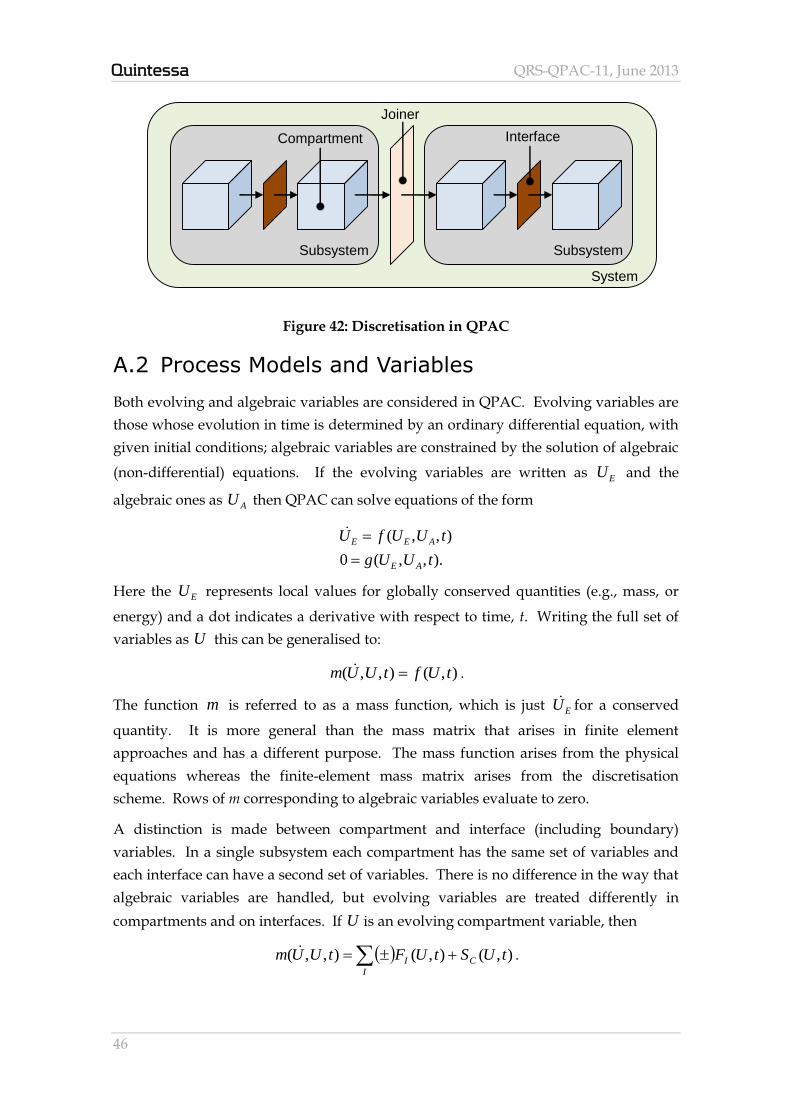
Appendix A: Technical Details

In this Appendix some of the key concepts discussed in Section 2 are described in more

detail. Information is given on the class of problems that QPAC can be applied to, but

users of Player versions of QPAC applications (see Section 2.3) do not need to be

familiar with the mathematical details.

A.1 System Discretisation

The modelled system can be broken down into a number of subsystems. Inside each

subsystem the set of processes to be modelled is defined. In a systems-level model,

separate subsystems will often be used to represent different parts of the system,

where the types of processes that are being modelled vary. In a detailed model,

separate subsystems can be used to break the system down in order to reduce the

amount of work to be done (i.e. reduce the number of variables to be solved for).

Each subsystem is broken down into compartments (sometimes referred to as control

volumes) with interfaces between these. In every compartment in a given subsystem

the set of processes that may be active is the same.

Subsystems can be linked by joiners. Joiners control how quantities simulated in one

subsystem affect, or are transported into, the other subsystem.

Collections of compartments corresponding to Cartesian or cylindrical polar grids can

be defined, or compartments can be specified individually (not in grids), which need

not necessarily have a fixed location in space and the collections need not be ‘space

filling’. Grids and individually specified compartments can both be used within the

same subsystem and their positions and volumes may change with time.

Discretisation in QPAC is illustrated in Figure 42.


46

Figure 42: Discretisation in QPAC

A.2 Process Models and Variables

Both evolving and algebraic variables are considered in QPAC. Evolving variables are

those whose evolution in time is determined by an ordinary differential equation, with

given initial conditions; algebraic variables are constrained by the solution of algebraic

(non-differential) equations. If the evolving variables are written as EU and the

algebraic ones as AU then QPAC can solve equations of the form

).,,(0

),,(

tUUg

tUUfU

AE

AEE

Here the EU represents local values for globally conserved quantities (e.g., mass, or

energy) and a dot indicates a derivative with respect to time, t. Writing the full set of

variables as U this can be generalised to:

),(),,( tUftUUm .

The function m is referred to as a mass function, which is just EU for a conserved

quantity. It is more general than the mass matrix that arises in finite element

approaches and has a different purpose. The mass function arises from the physical

equations whereas the finite-element mass matrix arises from the discretisation

scheme. Rows of m corresponding to algebraic variables evaluate to zero.

A distinction is made between compartment and interface (including boundary)

variables. In a single subsystem each compartment has the same set of variables and

each interface can have a second set of variables. There is no difference in the way that

algebraic variables are handled, but evolving variables are treated differently in

compartments and on interfaces. If U is an evolving compartment variable, then

),(),(),,( tUStUFtUUm C

I

I .

System

Subsystem Subsystem

Joiner

Compartment Interface


47

Here ),( tUSC are sources within the compartment (depending on variables within the

compartment) and ),( tUFI are fluxes across the compartment interfaces (depending

on variables on the interface and within the two compartments that share it).

Boundaries are treated as interfaces with only one associated compartment and fluxes

are applied consistently to the compartments connected by a given interface in order to

ensure conservation of the evolving variables. The source part of the equation can also

be used for reactions within a compartment, for example simple decay processes.

On an interface, evolving variables only have the source part of the equation; they can

be used, for example, to calculate an integrated flux over time across an interface.

The functional forms that can be used for the source and flux terms are completely

general, since QPAC allows any algebraic expression to be used to relate properties to

variables and then to use these properties in the specification of the sources and fluxes.

In summary, QPAC can solve a general system of differential and algebraic equations

within a compartmentalised system. The form of these equations is determined by the

particular model being implemented. The equations that QPAC solves need not arise

from a system of partial differential equations, but when a system of partial differential

equations is to be solved, the discretisation of these equations is part of the model

specification.

A.3 The Finite Volume Method

Although QPAC does not impose the approach that is to be used for spatially

discretising the system of partial differential equations (PDEs), the finite volume (or

control volume) approach is generally used (see, for example, Versteeg and

Malalasekra, 2007). It is possible to implement directly a finite-difference approach

and in simple cases this will lead to the same equations as the finite volume approach.

In the finite volume method, volume integrals in a PDE that contain a divergence term

can be converted to surface integrals, using the divergence theorem, enabling the

original partial differential equation to be replaced by ordinary differential equations

for the volume-averaged variables. Advantages of this approach include:

It does not require a structured grid, although a structured grid can be used.

Problems on irregular geometries can be considered.

Because the flux entering a given volume is identical to that leaving the

adjacent volume, variables are readily conserved.

Boundary conditions are easy to apply.

The alternative approach that is commonly used for continuum problems is the finite

element approach. This shares some of the advantages of the finite volume approach,


48

particularly in handling irregular geometries. The most significant difference between

the approaches is in the way that fluxes between volumes are treated. In the finite

volume approach there is a clear flux between volumes, ensuring that the relevant

quantity (e.g. mass) is conserved locally. In the finite element approach, there is no

unique flux between elements – the normal gradients will generally differ across the

interface – and local conservation is lost. For application areas where QPAC has been

used, local conservation of evolving quantities (such as mass) and the ability to see

how these are transported through the system are important – hence the choice of the

finite volume approach.

Consider, for example, a system of PDEs for a conserved quantity u

),(),( tuqtuJt

u

,

where J is a flux term and q is a source term. Within a particular volume (a

compartment), the above equation is solved in an averaged sense, so that

VVV

dVtuqdVtuJdVt

u),(),( .

Using the divergence theorem, this becomes

VVV

dVtuqdAntuJdVt

u),(),( ,

where V denotes the boundary of the volume, n is normal to that boundary and A is

the surface area.

The compartment variable relates to the volume integral

C

V

UdVu ,

the boundary of the volume is split into the various interfaces so that

I

I

FdAntuJ ),( ,

and the final sources and reactions term becomes the compartment source,

C

V

SdVtuq ),( .

Typically, the flux terms will involve local gradients which become differences in the

discretised scheme. This can be done with just compartment variables, taking

appropriate averages of any properties that are involved. The approach that is

generally taken in QPAC models is to define an interface variable to be an average of

the continuous variable on the interface and to use this in defining the flux on the

interface. The value of the interface variable is determined by imposing the required


49

flux consistently across an interface which gives a guarantee of conservation of mass or

energy.

The source term is commonly treated by using the averaged variable directly, so that

t

V

UVqS C

C , .

This implicitly assumes that the variable of interest is uniformly distributed in the

compartment. If this is known to be inappropriate, other averaging could be used and

the integral could be evaluated explicitly or approximately.

Where a compartment is adjacent to the external boundary, the flux term will be

determined by the boundary condition. If a Neumann (specified flux) condition

applies, then this is used directly. If a Dirichlet (fixed value) condition is specified,

then this determines the value of the interface variable and again is simply handled.

A.4 A Simple Example: Heat Conduction

A simple example to illustrate the general equations given above is given by modelling

heat conduction. The governing equation can be written in the following form:

sTt

cT

)(

Here T (K) is the temperature and (kg m-3), c (J kg-1 K-1) and (W m-1 K-1) are the

density, specific heat capacity and thermal conductivity of the medium respectively. A

source of heat is given by s (W m-3).

Within a compartment, k, which has volume Vk (m3) the total heat, kkk cTVH (J),

corresponds to UE in the general equations. Here we have assumed that the properties

are constant within compartments. The mass function m is simply the time derivative

of the total heat. The temperature, Tk, is an algebraic variable defined by the equation

linking it to the heat variable using the properties and c together with the relevant

volume Vk. The flux term is expressed in terms of the gradient of Tk, the property

and the relevant area A (m2). The source term for the compartment, Sk (W), is given by

the integral of s over the compartment. The gradient is approximated by a simple

difference formula, with the flux into neighbouring compartment l from compartment

k being given by

lk

lklklklk

d

TTAF

,

,,,

.

Here the subscripts denote evaluation at the interface between k and l and d (m) is the

distance between the compartment centres. Various schemes are possible for


50

determining the effective thermal conductivity to be used at the interface if the

properties are different on either side; the harmonic average of the transport

resistances / for the two compartments can be used, where is a representative

distance from the centre of the compartment to the interface between compartments.


51

Appendix B: Quality Assurance

The core QPAC code has been developed under the TickIT Quality Assurance system.

Maintenance of the software is facilitated by the use of an Issue Tracker where users

can identify bugs and development requests. This keeps an audit trail of relevant

activities from the time that the issue is raised to its resolution. Source control systems

are used to track changes to the source code, and every stage of the software lifecycle is

fully documented.

Module development is also managed according to Quality Assurance procedures

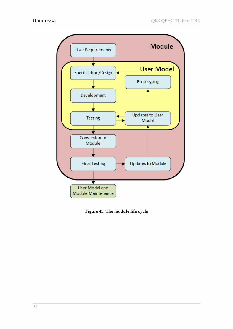
relevant to software development. The life-cycle of a module (with associated user

model(s)) follows the general format of the development life-cycle, as shown in Figure

43

QPAC applications have performed well in a number of international intercomparison

exercises (including the THERESA, DECOVALEX and FORGE projects referred to in

the main text) and the more the software is used in this way the more robust it will

become.

A number of peer-reviewed papers that include the use of QPAC simulations have

been published and examples of these are given in the references to the main text.

Verification of the core code is supported by the testing of a number of simple user

models. These demonstrate QPAC’s flexibility and application to different types of

problem.


52

Figure 43: The module life cycle

QPAC Overview Report

Documents

Transcript of QPAC Overview Report