QoS-enabled integration of wireless sensor networks · PDF fileQoS-enabled integration of...

Calhoun: The NPS Institutional Archive

Theses and Dissertations Thesis Collection

2005-09

QoS-enabled integration of wireless sensor networks

and the internet

AlMaharmeh, Bassam T.

Monterey, California. Naval Postgraduate School

http://hdl.handle.net/10945/1729

NAVAL

POSTGRADUATE SCHOOL

MONTEREY, CALIFORNIA

THESIS

QoS-ENABLED INTEGRATION OF WIRELESS SENSOR NETWORKS WITH THE INTERNET

by

Bassam AlMaharmeh

September 2005

Thesis Advisor: Su Weilian Second Reader: John C. McEachen

Approved for public release; distribution is unlimited

THIS PAGE INTENTIONALLY LEFT BLANK

i

REPORT DOCUMENTATION PAGE Form Approved OMB No. 0704-0188 Public reporting burden for this collection of information is estimated to average 1 hour per response, including the time for reviewing instruction, searching existing data sources, gathering and maintaining the data needed, and completing and reviewing the collection of information. Send comments regarding this burden estimate or any other aspect of this collection of information, including suggestions for reducing this burden, to Washington headquarters Services, Directorate for Information Operations and Reports, 1215 Jefferson Davis Highway, Suite 1204, Arlington, VA 22202-4302, and to the Office of Management and Budget, Paperwork Reduction Project (0704-0188) Washington DC 20503. 1. AGENCY USE ONLY (Leave blank)

2. REPORT DATE September 2005

3. REPORT TYPE AND DATES COVERED Master’s Thesis

4. TITLE AND SUBTITLE: QoS-Enabled Integration of Wireless Sensor Networks and the Internet

6. AUTHOR(S) Bassam AlMaharmeh

5. FUNDING NUMBERS

7. PERFORMING ORGANIZATION NAME(S) AND ADDRESS(ES) Naval Postgraduate School Monterey, CA 93943-5000

8. PERFORMING ORGANIZATION REPORT NUMBER

9. SPONSORING /MONITORING AGENCY NAME(S) AND ADDRESS(ES) N/A

10. SPONSORING/MONITORING AGENCY REPORT NUMBER

11. SUPPLEMENTARY NOTES The views expressed in this thesis are those of the author and do not reflect the official policy or position of the Department of Defense or the U.S. Government. 12a. DISTRIBUTION / AVAILABILITY STATEMENT Approved for public release; distribution is unlimited

12b. DISTRIBUTION CODE

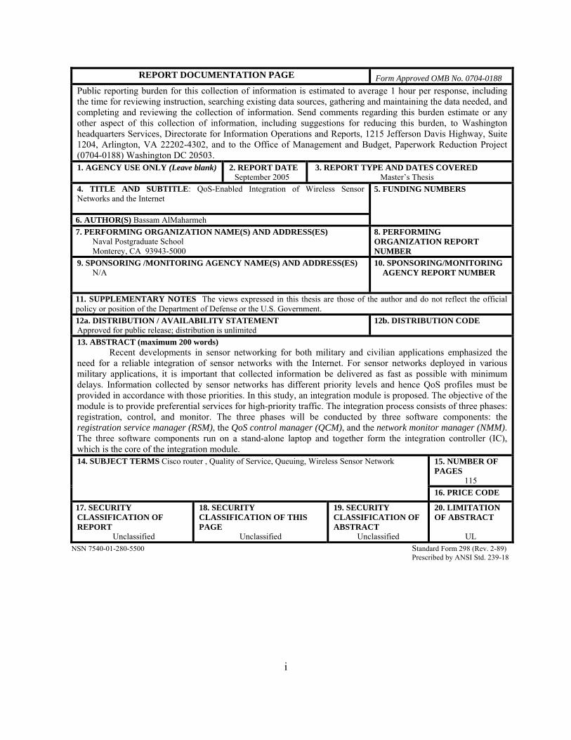
13. ABSTRACT (maximum 200 words) Recent developments in sensor networking for both military and civilian applications emphasized the

need for a reliable integration of sensor networks with the Internet. For sensor networks deployed in various military applications, it is important that collected information be delivered as fast as possible with minimum delays. Information collected by sensor networks has different priority levels and hence QoS profiles must be provided in accordance with those priorities. In this study, an integration module is proposed. The objective of the module is to provide preferential services for high-priority traffic. The integration process consists of three phases: registration, control, and monitor. The three phases will be conducted by three software components: the registration service manager (RSM), the QoS control manager (QCM), and the network monitor manager (NMM). The three software components run on a stand-alone laptop and together form the integration controller (IC), which is the core of the integration module.

15. NUMBER OF PAGES

115

14. SUBJECT TERMS Cisco router , Quality of Service, Queuing, Wireless Sensor Network

16. PRICE CODE

17. SECURITY CLASSIFICATION OF REPORT

Unclassified

18. SECURITY CLASSIFICATION OF THIS PAGE

Unclassified

19. SECURITY CLASSIFICATION OF ABSTRACT

Unclassified

20. LIMITATION OF ABSTRACT

UL

NSN 7540-01-280-5500 Standard Form 298 (Rev. 2-89) Prescribed by ANSI Std. 239-18

ii


iii

Approved for public release; distribution is unlimited

QoS-ENABLED INTEGRATION OF WIRELESS SENSOR NETWORKS AND THE INTERNET

Bassam T. AlMaharmeh Major, Army, Hashemite Kingdom of Jordan

B.S., Mu’tah University, Jordan, 1989

Submitted in partial fulfillment of the requirements for the degree of

MASTER OF SCIENCE IN ELECTRICAL ENGINEERING

from the

NAVAL POSTGRADUATE SCHOOL September 2005

Author: Bassam AlMaharmeh

Approved by: Weilian Su

Thesis Advisor

John C. McEachen Second Reader

Jeffrey Knorr Chairman, Department of Electrical and Computer Engineering

iv


v

ABSTRACT

Recent developments in sensor networking for both military and civilian

applications emphasized the need for a reliable integration of sensor networks with the

Internet. For sensor networks deployed in various military applications, it is important

that collected information be delivered as fast as possible with minimum delays.

Information collected by sensor networks has different priority levels and hence QoS

profiles must be provided in accordance with those priorities. In this study, an integration

module is proposed. The objective of the module is to provide preferential services for

high-priority traffic. The integration process consists of three phases: registration,

control, and monitor. The three phases will be conducted by three software components:

the registration service manager (RSM), the QoS control manager (QCM), and the

network monitor manager (NMM). The three software components run on a stand-alone

laptop and together form the integration controller (IC), which is the core of the

integration module.

vi


vii

TABLE OF CONTENTS

I. INTRODUCTION........................................................................................................1 A. BACKGROUND ..............................................................................................1 B. OBJECTIVES ..................................................................................................3 C. RELATED WORK ..........................................................................................3 D. THESIS ORGANIZATION............................................................................4

II. QOS OVERVIEW .......................................................................................................7 A. INTRODUCTION............................................................................................7 B. QoS SERVICE MODELS ...............................................................................8

1. Best-Effort Service ...............................................................................8 2. Integrated Service ................................................................................8

a. First-In-First-Out Queuing (FIFO).......................................11 b. Fair Queuing (FQ)..................................................................11 c. Weighted Fair Queuing (WFQ) .............................................12 d. Class-Based Weighted Fair Queuing (CBWFQ)...................14 e. Priority Queuing (PQ) ............................................................15 f. Random Early Detection (RED).............................................16

3. Differentiated Services.......................................................................17 C. QOS IMPLEMENTATION IN THE INTEGRATION BETWEEN

THE INTERNET AND WIRELESS SENSOR NETWORKS ..................20 D. SUMMARY ....................................................................................................21

III. WIRELESS SENSOR NETWORKS OVERVIEW ...............................................23 A. INTRODUCTION..........................................................................................23 B. WIRELESS SENSOR NETWORK CHALLENGES ................................26 C. WIRELESS SENSOR NETWORKS REQUIREMENTS .........................27 D. WIRELESS SENSOR NETWORKS APPLICATIONS............................29 E. WIRELESS SENSOR NETWORKS ROUTING TECHNIQUES ...........30 F. SENSOR NETWORK PLATFORMS .........................................................31

1. Sensor Node Hardware......................................................................31 2. Operating System: TinyOS ...............................................................33

G. SUMMARY ....................................................................................................34

IV. INTEGRATION ARCHITECTURE.......................................................................35 A. INTRODUCTION..........................................................................................35 B. PROPOSED INTEGRATION MODULE OVERVIEW ...........................35 C. HARDWARE AND SOFTWARE COMPONENTS ..................................37

1. Wireless Sensor Networks.................................................................37 2. Access Point ........................................................................................38 3. Applications ........................................................................................38 4. Edge Routers (Cisco™ 2651 and 2811)............................................39 5. Integration Controller (IC) ...............................................................40

D. THE REGISTRATION SERVICE MANAGER (RSM)............................41

viii

E. THE NETWORK MONITOR MANAGER (NMM)..................................42 1. The Periodic Update Message...........................................................42 2. The Event-driven Message ................................................................45

F. QOS CONTROL MANAGER (QCM) ........................................................45 1. The initialization phase......................................................................47 2. Self-adaptation phase.........................................................................47

a. Bandwidth Allocation Algorithm (BAA)................................48 b. Traffic policing and shaping ..................................................50 c. The response to network congestions and link failures ........51

G. WIRELESS SENSOR NETWORKS REGISTRATION PROTOCOL (WSNRP) ........................................................................................................51

H. SUMMARY ....................................................................................................52

V. PERFORMANCE ANALYSIS.................................................................................53 A. INTRODUCTION..........................................................................................53 B. LABORATORY SETUP...............................................................................53

1. Equipment and software components..............................................53 2. Procedures ..........................................................................................55 3. Expectations........................................................................................57

C. DATA COLLECTION AND ANALYSIS TOOLS ....................................60 D. RESULTS AND ANALYSIS ........................................................................60

1. Throughput.........................................................................................60 2. Video flow analysis.............................................................................63 3. Audio flow analysis ............................................................................64 4. Sensitive data flow analysis ...............................................................65 5. Non-sensitive data flow analysis .......................................................68 6. Response time analysis ......................................................................70

a. The processing delay at the NMM..........................................70 b. The processing delay at the QCM...........................................71 c. Connection set-up time ...........................................................71 d. Response time of the router ....................................................71

E. THE CONTRIBUTION OF THE WSNRP IN MINIMIZING TRAFFIC........................................................................................................72

F. SUMMARY ....................................................................................................76

VI. CONCLUSIONS AND FUTURE WORK...............................................................77 A. INTRODUCTION..........................................................................................77 B. CONCLUSION ..............................................................................................77 C. FUTURE WORK...........................................................................................78

1. Adding a security component ...........................................................78 2. More investigation on the response time .........................................79 3. Modeling the traffic of sensor networks ..........................................79 4. Using real data from sensor nodes ...................................................79

APPENDIX A. WIRELESS SENSOR NETWORK REGISTRATION PROTOCOL (WSNRP).............................................................................................81 A. OVERVIEW...................................................................................................81

ix

B. TYPES OF MESSAGES ...............................................................................81 1. Registration Request Message ..........................................................81 2. Update Message..................................................................................82

C. REGISTRATION SEQUENCE ...................................................................82 D. MESSAGE FORMAT ...................................................................................83

1. Header.................................................................................................83 a. Request ID...............................................................................84 b. Request/Response (RR)...........................................................84 c. Request Type (RT)...................................................................84 d. Client Type (CT)......................................................................85 e. Priority Level (P).....................................................................85 f. Topics Count ...........................................................................85

2. Message Contents...............................................................................85 a. Message Content of the Request Message .............................85 b. Message Content of the Response Message ...........................86

E. REGISTRATION INFORMATION FILE (RIF).......................................87

APPENDIX B. QOS INITIAL PROFILE .................................................................89

LIST OF REFERENCES......................................................................................................91

INITIAL DISTRIBUTION LIST .........................................................................................95

x


xi

LIST OF FIGURES

Figure 1. Integrated Services Architecture ISA Implemented in Router (From Ref. 12) ....................................................................................................................10

Figure 2. Fair Queuing ....................................................................................................12 Figure 3. Weighted Bit-by-Bit Round-Robin Scheduler wit Packet Assembler.............13 Figure 4. Weighted Fair Queuing (WFQ) Service According to Packet Finish Time ....13 Figure 5. Class-Based Weighted Fair Queuing...............................................................15 Figure 6. Priority Queuing (From Ref. 9) .......................................................................16 Figure 7. Weighted Random Early Detection (From Ref. 9) ..........................................17 Figure 8. The DS field structure (From Ref. 17).............................................................18 Figure 9. DS Domains (From Ref. 12)............................................................................19 Figure 10. Protocol Stack for 802.15.4 and ZigBee..........................................................24 Figure 11. Wireless standards, Data Rates vs. Range .......................................................25 Figure 12. The Components of the Wireless Sensor Network, where BST is the Base

Station (After Ref. 22) .....................................................................................29 Figure 13. MICA Mote Architecture (After Ref. 18)........................................................33 Figure 14. The Proposed Integration Module ...................................................................36 Figure 15. The Three Phases of the Integration Process ...................................................37 Figure 16. Cisco™ 2651XM Router Front and Rear Panels (From Ref. 32)....................39 Figure 17. Cisco™ 2811 Router (From Ref. 33) ..............................................................40 Figure 18. The Interactions between the Software Modules.............................................41 Figure 19. Round-Trip Delay Exercised by Traffic Using Different Queuing Systems...46 Figure 20. Number of Dropped Packets for Traffic Using Different Queuing Systems...46 Figure 21. Bandwidth Allocation Algorithm (BAA) ........................................................48 Figure 22. The Normalized Allocated Bandwidth with respect to R/RT at different

W/WT ................................................................................................................50 Figure 23. The Laboratory Setup ......................................................................................54 Figure 24. Throughput of the Network (Fair Queuing).....................................................61 Figure 25. Throughput of the Network (Integration Controller).......................................62 Figure 26. Inter-arrival Time Distribution of the Video Flow (Fair Queuing) .................63 Figure 27. Inter-arrival Time Distribution of the Video Flow (Integration Controller)....64 Figure 28. Delay of the Audio Flow (Fair Queuing).........................................................65 Figure 29. Delay of the Audio Flow (Integration Controller)...........................................65 Figure 30. Round-trip Time (RTT) of the Sensitive Data Flow (Fair Queuing)...............66 Figure 31. Round-trip Time (RTT) of the sensitive Data Flow (Integration Controller)..66 Figure 32. Round-trip Time (RTT) Cumulative Distribution Function for the

Sensitive Data Flow under the Fair Queuing System (FQ) .............................67 Figure 33. Cumulative Distribution Function of Round-trip Time of the Sensitive

Data Flow (Integration Controller) ..................................................................68 Figure 34. Delay of the Non-sensitive Data Flow (Fair Queuing)....................................68 Figure 35. Delay of the Non-sensitive Data Flow (Integration Controller) ......................69

xii

Figure 36. Dropped Packets the Non-sensitive Data Flow under the Control of the Integration Controller (IC)...............................................................................70

Figure 37. N-Applications and K-WSNs...........................................................................73 Figure 38. The Maximum Reduction (Qmax) in Request Messages...................................75 Figure 39. The Location of WSNRP in the TCP/IP Stack ................................................81 Figure 40. The Registration Process Sequence .................................................................82 Figure 41. WSNRP Header Format Without Showing the Content Fields .......................84 Figure 42. WSNRP Header Format for the Client Request Message ...............................86 Figure 43. WSNRP Format of the RSM Server’s Response Message..............................87 Figure 44. Sample output of the RIF.................................................................................87

xiii

LIST OF TABLES

Table 1. Key Attributes Comparison of Wireless Networks .........................................26 Table 2. The Contents of The NMM’s Periodic Update Message.................................43 Table 3. Mapping Between Priority Classes and Precedence Levels ............................43 Table 4. Weights Assignment Based on Flow’s Class and Data Rate...........................44 Table 5. The Characteristics of the Data Flows .............................................................57 Table 6. Criteria used by the BAA to Allocate Bandwidth for the Traffic during the

First Five Minutes of the Experiment (First Iteration).....................................58 Table 7. Criteria used by the BAA to Allocate Bandwidth for the Traffic during the

First Five Minutes of the Experiment (Second Iteration) ................................58 Table 8. Criteria used by the BAA to Allocate Bandwidth for the Traffic during the

Second Five Minutes of the Experiment (First Iteration) ................................59 Table 9. Criteria used by the BAA to Allocate Bandwidth for the Traffic during the

Second Five Minutes of the Experiment (Second Iteration)............................59 Table 10. Perl Scripts Used to Extract Statistical Information from Collected Packets..60 Table 11. The Request Type Options...............................................................................84 Table 12. Client Type Options.........................................................................................85

xiv


xv

ACKNOWLEDGMENTS

I would like to express my sincere appreciation to Prof. Su Weilian for his helpful

advice and providing the necessary equipments and resources. His encouragement and

support kept me on track.

I would like also to thank Prof. John McEachen for his time and effort in

reviewing this thesis.

Finally, I would like to thank my wife, Fatima Musa, for being always there to

support me through my work.

xvi


xvii

EXECUTIVE SUMMARY

An integration module is proposed in this study. The integration module core

component is the integration controller (IC), which is a stand-alone laptop with three

software modules running on top of it: the registration service manager (RSM), the QoS

control manager (QCM), and the network monitor manager (NMM). The three software

modules work together to register traffic at the integration link, monitor it, and then

provide an adaptive QoS. The integration module’s objective is to provide high-priority

traffic with preferential service, while maintaining other lower priority traffic.

The RSM receives registration requests from applications on the Internet in order

to access the available WSNs. The registration is carried out with help of the wireless

sensor network registration protocol (WSNRP), which is presented in this thesis.

The NMM monitors the traffic in the integration link and sends statistical

information about each flow to the QCM. Also, the NMM informs the QCM about

congestion and link failures.

Based on the registration and monitoring information, the QCM adapts the QoS

configurations at the edge router in such a way that helps high-priority traffic to be

delivered with minimum delay. The QCM uses class-based weighted fair queuing

(CBWFQ) and priority queuing (PQ) to provide differential services. The QCM allocates

class-based bandwidth for each flow using a simple algorithm (i.e., bandwidth allocation

algorithm - BAA).

A simulation network was set up in the Advanced Networking Laboratory at the

Naval Postgraduate School. The goals of the simulation network were to test and measure

the performance of the integration module and compare it with the performance of the

fair queuing system. Four flows with different characteristics were used to simulate the

sensor network traffic. The four flows were: high-priority video flow, high-priority audio

flow, normal-priority non-sensitive data flow, and urgent-priority sensitive data flow.

xviii

The results obtained from the simulation showed an improved performance of

high-volume flows compared with their performance at the FQ system. The performance

of the urgent flow was improved by 55.5%. Also, the results showed that the integration

module was less affected by sudden traffic bursts. When the high data rate burst was

injected into the network, it had a small effect on the high-volume flows’ throughput

compared with the FQ system.

The throughput of the unwanted normal-priority flow was suppressed by 45%

under the integration module, which minimized its effect on other higher priority flows.

The performance of low-volume flows were almost the same under the two

systems (integration controller and FQ). This is because the two systems allocate

sufficient bandwidth for low-volume traffic.

The response time of the integration module was only discussed briefly in this

study. The integration module’s response time consisted of several delay times, which

included the processing time at both the QCM and the NMM, the connection setup time

with the router, and the router’s response time for changes on its configuration file.

1

I. INTRODUCTION

A. BACKGROUND Thanks to significant technological advances in integrated circuit technology, the

miniaturization of electronics has produced a far-reaching technological revolution in the

sensors industry, which has enabled construction of far more capable yet inexpensive

sensors, processors, and radios. Currently, very tiny sensors are produced commercially

for a wide range of applications, and range from habitat and ecological sensing, structural

monitoring and smart spaces, to emergency response and remote surveillance [1][2]. It is

expected that within the next few years, the size of sensor nodes will continue to shrink,

and sensor networks may cover the globe resulting in hundreds of thousands of wireless

sensor networks (WSNs) scattered over battlefields, large farms, and warehouses

collecting motion, changes in temperatures and other important information. One of the

major forces that is pushing the industry of sensor networking forward is the retailer

business and the idea of using radio frequency ID tags (RFID) as next generation

barcodes that will allow RF readers to collect information about inventory.

Wireless sensor networks have tremendous potential for applications in the

military field, and several military applications will take advantage of the great and

unique opportunities introduced by WSNs. Low-power sensor nodes can be used to

collect information from the frontlines of the battlefields about enemy forces movements,

locations of missile launchers and artillery batteries, and many other targets. This can be

achieved by dispersing a large number of sensor nodes into the target area, where the

scattered nodes start communicating using embedded RF transceivers with very low

power. The sensor nodes may group together in hierarchal clusters to facilitate the task of

information collection and forwarding.

Wireless sensor networks promise an enormous extension of the Internet. For the

time being, the Internet is a collection of human made products like numbers, images,

music, and videos. With sensor networks extensions, activities over the globe will be

monitored and millions of new sensor networks will change the face of the Internet.

2

One main issue in WSNs is to deliver the collected information efficiently with

minimum delays to data centers, where different pieces of information are brought

together in order to build the big picture. This can be achieved by employing existing

Quality of Service (QoS) techniques into the integration between WSNs and the Internet.

The integration of WSNs and the Internet is becoming more and more important

because of the numerous numbers of WSNs that will join the Internet domain. Currently,

the data gathered by WSNs are delivered to data centers with best-effort services, which

means that delay-sensitive and time-sensitive data is subject to be dropped or delayed in

congested networks. With best-effort integration, low-volume traffic is leapfrogged by

high-volume applications and there is no guarantee that short sensor network's alert

messages and events will be delivered. However, with QoS-enabled integration, time-

sensitive data and delay-sensitive applications are guaranteed to have preferential service

through the implementation of certain QoS techniques provided by network components

such as routers.

Unfortunately, the only QoS functionality provided by the Internet Protocol (IP) is

the Type of Service (TOS) field, which is used to classify the traffic into different classes

defined in the IP standards RFC-791 [3]. The problem with TOS is that it is rarely used,

and in most cases, the TOS field is reset at different network nodes. The nature of the

data in the domain of WSNs requires more QoS functionalities, which are beyond the

TOS capabilities.

The data exchanged between WSNs and the Internet has its own characteristics,

where a mixture of high-importance small-alert packets and routine request messages

coexist. The 802.15.4 standards defined the data rate for sensor nodes to be in the range

20-250 Kbps. Therefore, sensor nodes generate low data rate traffic streams in either

proactive or reactive transmission modes. Data sent by sensor nodes are aggregated and

forwarded to the base station or the gateway. Compared to Internet traffic, the sensor

network’s aggregated traffic streams occupy smaller bandwidths. QoS technologies that

exist today are designed for the Internet, where congestion and long delays are common.

This thesis, will experiment with the suitability of those QoS techniques for the traffic of

WSNs.

3

Reliability of the collected information is also an important element that

characterizes the wireless sensor network's traffic and requires techniques to ensure the

delivery of highly reliable information that satisfies the applications' needs. With all these

requirements and challenges in mind, an integration module is introduced in this thesis

that addresses the challenges in the integration effort of WSNs and the Internet. The

proposed integration module assumes that one or more WSNs are connected to the

Internet through a QoS-capable router, which will work cooperatively with the

integration controller (IC). The IC is a PC or laptop that has three software components:

registration server module (RSM), QoS control manager (QCM), and network monitor

manager (NMM). In order to address the discussed challenges, the integration module

suggests that both the applications interested in sensor's data (sensor-applications) and the

WSNs register with the RSM through the Wireless Sensor Network Registration Protocol

(WSNRP). The QCM is the intelligent component that adapts the network parameters,

such as bandwidth and queuing, in such a way that ensures the provision of the proper

level of QoS. This can be achieved by working cooperatively with the other two modules,

the RSM and the NMM. The NMM is a module that continuously monitors the

integration link between the WSN and the Internet, looking for changes in traffic patterns

and traffic bursts. Then the monitoring information will be used by the QCM to adapt the

network parameters with any changes.

B. OBJECTIVES The objective of this thesis is to develop an integration module for the integration

between WSNs and the Internet. The proposed Integration Module guarantees reliable

and smooth flow of critical information between the Internet and WSNs by employing a

set of QoS techniques and controls. The suitability of currently available QoS techniques

will be examined in the proposed integration module. As part of the integration module,

the WSNRP is introduced in this thesis.

C. RELATED WORK In order to efficiently integrate WSNs and the Internet, a tremendous research

effort had to be focused on a management architecture for WSNs. Several references

focused on the implementation of clustering hierarchy of sensors. In this scenario, sensors

are grouped into clusters, and each cluster has one designated node that serves as a

4

‘gateway’ to the Internet or to another gateway (in multi-hop networks) [4][5][6]. Some

references even proposed hierarchies that employ, in addition to cluster-heads at the low-

level, cluster-managers at the top-level to facilitate the transport of information and to

minimize unnecessary traffic which in turn will maximize the bandwidth utilization. In

[2], the authors suggested the use of gateway(s) or the overlay of IP networks between

the WSNs and the Internet and ruled out the possibility of all-IP sensor networks, because

of the characteristics of WSNs that differentiate them from traditional IP-based networks,

such as WSNs are large-scale unattended systems consisting of resource-constrained

nodes that are best-suited to application-specific, data-centric routing. In addition, they

concluded that all-IP networks are not viable with the new technology of WSNs due to

the fundamental differences in the architecture of IP-based networks and WSNs. The

authors pointed out that the basic solution for integration in the case of a homogeneous

WSN, where all the nodes have the same capability in terms of processing, energy and

communication resources, is to use an application-level gateway, and for heterogeneous

networks, is to use an overlay network based on a flooded-query approach that use

directed diffusion [7]. In this thesis, this approach will be used, and WSNs will be

accessed through an application-layer gateway.

Using the TCP/IP protocol stack within sensor networks would have facilitated

their integration with the Internet, but unfortunately TCP/IP is a heavy-weight protocol

stack that cannot be implemented in tiny sensors with limited resources. Therefore, the

Swedish Institute of Computer Science SICS is developing a light-weight TCP/IP

protocol stack called µIP that is small enough to be used in sensor networks, and also

allows for spatial IP address assignment where each sensor constructs its IP address from

its physical location [8]. The proposed solution from SICS also introduces other features

like shared context header compression to overcome the large overhead of TCP/IP. Also,

they presented the usage of application overlay networking to solve the problem of

addressing in WSNs [9].

D. THESIS ORGANIZATION The thesis is divided into six chapters. Chapter I is an introduction. In Chapter II,

a review of QoS concepts and techniques is presented, which also includes a discussion

on Cisco™ IOS’s QoS capabilities. In Chapter III, an overview of the wireless sensor

5

networks is presented. In Chapter IV, the architecure of the proposed integration module

is introduced and discused, and this includes both the hardware and software architecures

in addition to a discussion on the proposed Wireless Sensor Networks Registration

Protocol. In Chapter V, a performance analysis of the integration module is presented,

and includes the performance experiments and tests conducted during the analysis

process. Lastly, the thesis is concluded and future recommendations are presented in

chapter VI. Appendix A contains a detailed description of the Wireless Sensor Networks

Registration Protocol. Appendix B contains the intial QoS profile.

6


7

II. QOS OVERVIEW

A. INTRODUCTION There are a number of definitions available in textbooks and on the Web. The

following is a list of definitions found at different resources:

1. Cisco™ Systems: “QoS is the capability of a network to provide better

service to selected network traffic over various technologies. [10]”

2. Microsoft™ Corp: “QoS: is a set of service requirements that the network

must meet in order to ensure a adequate service level for data

transmission. [11]”

3. The International Telecommunication Union (ITU):”QoS is the collective

effect of service performance which determines the degree of satisfaction

of a user of the service” [12]

4. The Internet Engineering Task Force IETF: RFC 1946, Native ATM

Support for ST2+, states "As the demand for networked real time services

grows, so does the need for shared networks to provide deterministic

delivery services. Such deterministic delivery services demand that both

the source application and the network infrastructure have capabilities to

request, setup, and enforce the delivery of the data. Collectively these

services are referred to as bandwidth reservation and Quality of Service

(QoS)." [13].

QoS is not an essential component for all applications, especially those

applications that are not delay-sensitive like Telnet and FTP. Currently, the Internet

offers end-to-end delivery service, without any guarantee regarding bandwidth and

latency. The best TCP can do is provide reliable delivery, which might be sufficient for

delay-insensitive applications, but not for applications requiring timeliness like voice and

video applications and others that are sensitive to delays. Bandwidth is expensive and

needs to be used efficiently to avoid long idle periods and at the same time to avoid

congestion periods. QoS can be thought of as the network traffic policeperson who

ensures a smooth flow of traffic.

8

QoS can help by smoothing the traffic and using the bandwidth more efficiently

in certain cases. However, it cannot solve a vastly over-utilized link with limited

bandwidth and bottlenecks. Another important point is the fact that voice and video and

other delay-sensitive applications are fragile traffic and can be easily impacted by large

file transfers and traffic bursts that can easily fill output buffers and cause packets to be

dropped. QoS should address all these issues and ensure that fragile packets are not

overwhelmed by heavyweight traffic.

B. QoS SERVICE MODELS QoS service models describe the level of service to be delivered. They differ from

one another in how they attempt to deliver the data among applications. Each service

model is appropriate for certain applications. Therefore, it is important to consider the

available applications when deciding which type of service model to deploy. Another

factor to be considered is the cost of each service model. There are generally three QoS

service models which can be deployed in the network [14]:

• Best-effort service

• Integrated service

• Differentiated service

1. Best-Effort Service Best-effort service is one that does not provide full reliability. Applications

normally send data whenever they must in any quantity and without first informing the

network. In this type of service, data is delivered without any insurance of reliability,

delay, or throughput.

It is true that best-effort service is unreliable, but at the same time its inherent

feature is one of the most powerful strengths. It is simple and scalable in such a way that

it enabled the expansion of the Internet over the entire globe. Best-effort service is

suitable for a large number of Internet applications such as FTP, SMTP, and many others.

One of the technologies that implements best-effort service is first-in-first-out queuing.

2. Integrated Service The IPv4 header is equipped with fields that can specify precedence and type of

service as described in RFC 791 “Internet Protocol” [3], but unfortunately those fields

have generally been ignored by routers in selecting routes and treating individual packets.

9

In IP-based networks, multimedia and multicasting applications are not well supported,

because IP was fundamentally built to transmit data among local area networks (LANs).

The only network that was designed from day one to support real time traffic is ATM

[14]. However, neither building new ATM networks for real-time traffic nor replacing

existing IP-based networks with ATM is cost effective.

Thus, the solution is to support a variety of applications, which includes real-time

service, and implement QoS techniques within the TCP/IP networks. The Internet

Engineering Task Force (IETF) developed a suite of standards for the Integrated Services

Architecture (ISA), which was intended to provide QoS over IP-based networks. The

standards are defined in RFC 1633.

The most important factors that QoS should address are:

a. Throughput: Some applications require a minimum throughput to be

available in order to work properly, while others can continue to work but

with degraded service.

b. Delay: stock trading is a good example on delay-sensitive applications.

c. Jitter: It is the magnitude of packet interarrival variations. Some

applications require reasonable upper bounds on jitter.

d. Packet Loss: Different applications have different requirements for packet

loss, and this includes the real-time applications.

In order to meet the above factors, some means are needed to give preferential

treatment to applications with high-demand requirements. Therefore, applications are

obligated to state their requirements either ahead of time, in some sort of reservation

requests, or on the fly using some fields in the IP packet header. The first approach is

more flexible, because it enables the network to anticipate demands and deny new

requests if resources are not available. In this case, a resource reservation protocol is

needed. Resource ReSerVation Protocol RSVP [15] was designed for this purpose as well

as to be an integral component of an ISA.

ISA is an architecture that enhances the performance of best-effort networks by

applying some new techniques. In ISA, packets are considered part of flows, where a

flow is distinguished as a stream of related IP packets that results from a single user

activity and requires the same QoS [14]. The following is a description of ISA

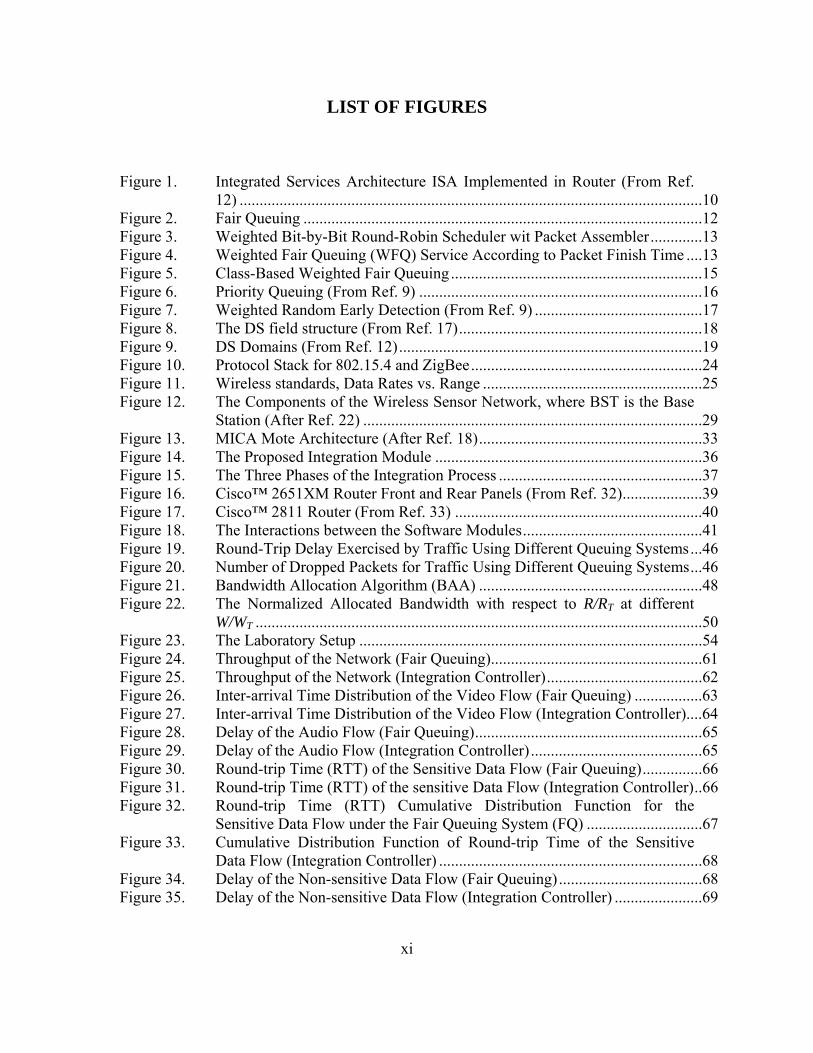
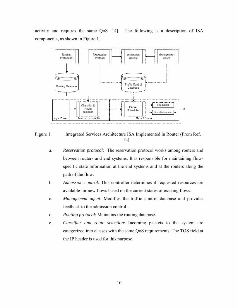
components, as shown in Figure 1.

Figure 1. Integrated Services Architecture ISA Implemented in Router (From Ref. 12)

a. Reservation protocol: The reservation protocol works among routers and

between routers and end systems. It is responsible for maintaining flow-

specific state information at the end systems and at the routers along the

path of the flow.

b. Admission control: This controller determines if requested resources are

available for new flows based on the current states of existing flows.

c. Management agent: Modifies the traffic control database and provides

feedback to the admission control.

d. Routing protocol: Maintains the routing database.

e. Classifier and route selection: Incoming packets to the system are

categorized into classes with the same QoS requirements. The TOS field at

the IP header is used for this purpose.

10

11

f. Packet scheduler: Manages and controls the queues for each output port. It

determines the order of transmissions and determines the packets to be

dropped. It also polices the flows and monitors for violations in the

committed capacities of the flows.

Most network devices have one or more queuing disciplines that are used in

output ports to prepare packets for transmission into the medium. The traditional queue

scheduling disciplines that are considered here include First-In-First-Out Queuing

(FIFO), Fair Queuing (FQ), Weighted Fair Queuing (WFQ), Class-Based Weighted Fair

Queuing (CBWFQ) and Priority Queuing (PQ). These will be discussed in more detail

below.

a. First-In-First-Out Queuing (FIFO) Traditionally, routers implement the first-in-first-out (FIFO) queuing

system, where each output port has a single queue and packets are served on first-come-

first-served basis with no special treatment given to high-priority packets. Small packets

normally experience long delays, especially when the network is overwhelmed with large

packets from applications like FTP. In order to give preferential service for high-priority

packets, other queuing disciplines are used.

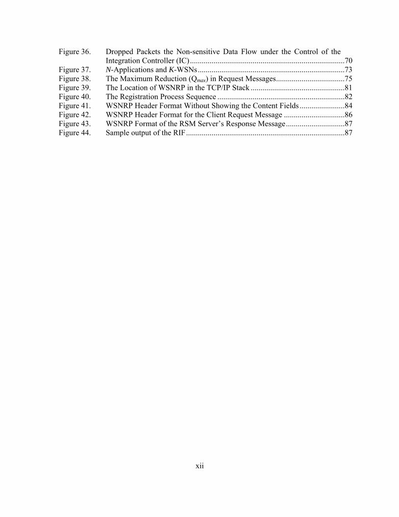
b. Fair Queuing (FQ) Fair queuing discipline was proposed by Nagle [16]. In this discipline,

routers maintain multiple queues for each output port. Each flow could have a separate

queue. In this case, packets are queued according to the flows they belong to. For one

cycle, each queue sends one packet in a round-robin fashion. Queues for heavyweight

flows become long and experience longer delays. In FQ, QoS for flows do not degrade

due to the bursting or misbehaving nature of other flows, because flows are isolated in

different queues.

One of the drawbacks of FQ is its sensitivity to the order of arrival. If a

packet has arrived at an empty queue and just missed the round-robin scheduler, then the

packet has to wait for a full round-robin cycle. Also, FQ does not have a mechanism to

support real-time applications like VoIP. FQ assumes that classification of flows is easy,

which has turned out in several cases not to be true. Finally, FQ spends more time

transmitting long packets than short packets, so applications that primarily transmit short

packets are penalized. Figure 2 shows how FQ works with multiple input flows, where

each flow is queued separately.

CLA

SSIF

IER

SCH

EDU

LER

PORT

Flow 1

Flow 2

Flow 3

Flow 4

Flow 5

Flow 6

Flow 7

Figure 2. Fair Queuing

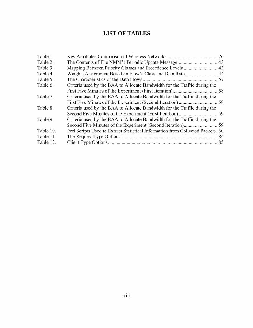
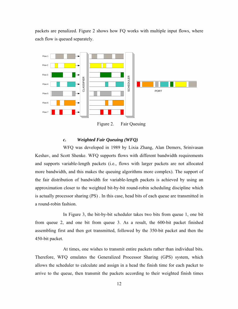
c. Weighted Fair Queuing (WFQ) WFQ was developed in 1989 by Lixia Zhang, Alan Demers, Srinivasan

Keshav, and Scott Shenke. WFQ supports flows with different bandwidth requirements

and supports variable-length packets (i.e., flows with larger packets are not allocated

more bandwidth, and this makes the queuing algorithms more complex). The support of

the fair distribution of bandwidth for variable-length packets is achieved by using an

approximation closer to the weighted bit-by-bit round-robin scheduling discipline which

is actually processor sharing (PS) . In this case, head bits of each queue are transmitted in

a round-robin fashion.

In Figure 3, the bit-by-bit scheduler takes two bits from queue 1, one bit

from queue 2, and one bit from queue 3. As a result, the 600-bit packet finished

assembling first and then got transmitted, followed by the 350-bit packet and then the

450-bit packet.

At times, one wishes to transmit entire packets rather than individual bits.

Therefore, WFQ emulates the Generalized Processor Sharing (GPS) system, which

allows the scheduler to calculate and assign in a head the finish time for each packet to

arrive to the queue, then transmit the packets according to their weighted finish times

12

(i.e., the packet with the theoretical earliest finish time within its priority class will be

transmitted first). Bit-round Fair Queuing (BRFQ) emulates a bit-by-bit round-robin

discipline but whole packets are forwarded in each round. WFQ is BRFQ with weighting

Wei

ghte

d Bi

t-by-

Bit R

ound

Rob

inSc

hedu

ler

600 bits

350bits

450 bits

Queue 2 (25% of BW)

Queue 3 (25% of BW)

Queue 1 (50% of BW)

Last bit of 450-bitpacket



PacketAssembler

450 350 600

Figure 3. Weighted Bit-by-Bit Round-Robin Scheduler wit Packet Assembler

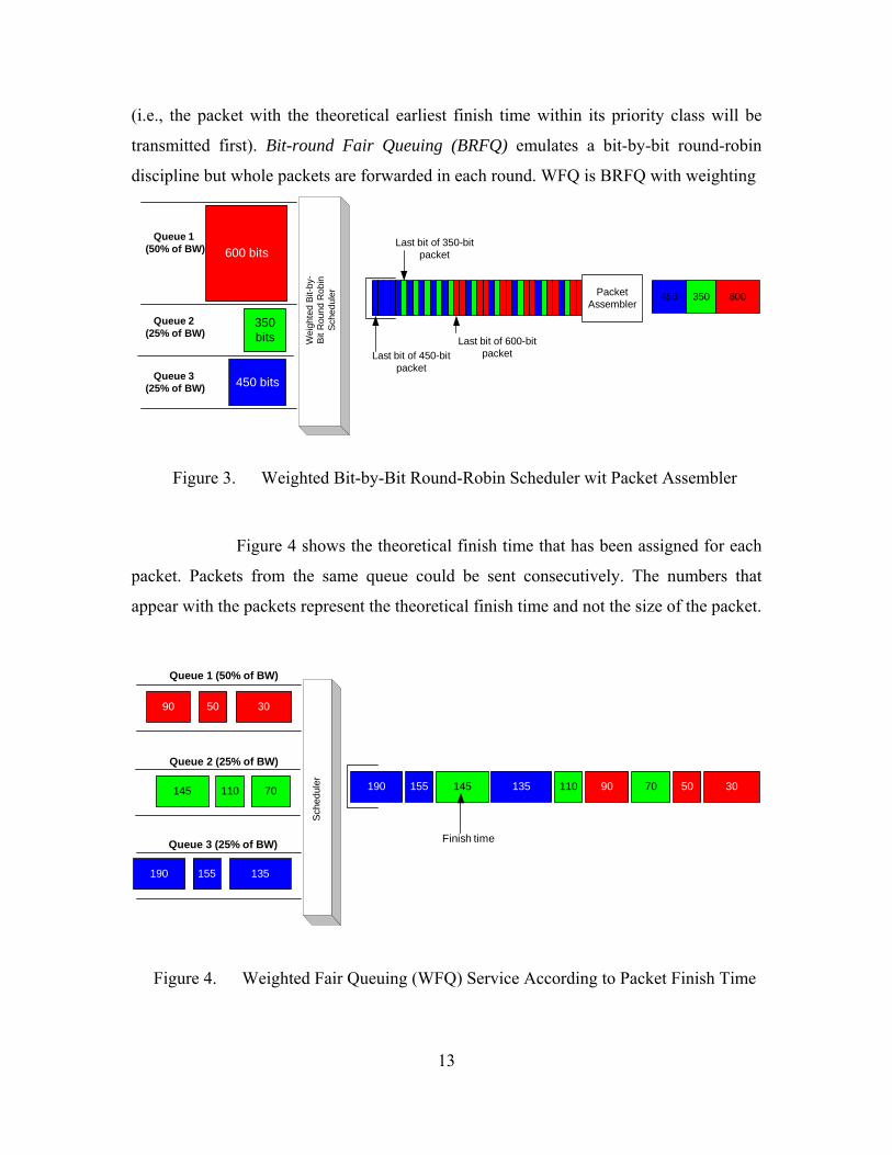
Figure 4 shows the theoretical finish time that has been assigned for each

packet. Packets from the same queue could be sent consecutively. The numbers that

appear with the packets represent the theoretical finish time and not the size of the packet.

Sche

dule

r

Queue 2 (25% of BW)

Queue 3 (25% of BW)

Queue 1 (50% of BW)

Finish time

305090

110145

135155190

305070 7090110135145155190

Figure 4. Weighted Fair Queuing (WFQ) Service According to Packet Finish Time

13

Cisco™ implements WFQ in most of their routers. Usually, routers

classify the traffic at the network edge into different flows based on several factors, such

as, source and destination addresses, protocol, source and destination port and socket

numbers, and ToS value. Cisco™ implementation divides the traffic into two main flows:

high-bandwidth sessions and low-bandwidth sessions. Low-bandwidth traffic has a

priority over the high-bandwidth traffic. Also, Cisco™ uses the IP precedence bits in the

IP header to classify flows, and as the precedence of the traffic increases, WFQ allocates

more bandwidth to the conversation during periods of congestion. WFQ assigns weights

for each flow, which equal to the precedence of the flow plus one, and then this weight is

used to determine when the packet will be serviced. For example, if there is one flow at

each precedence level, each flow will get its precedence + 1 part of the link. Weights in

Cisco™ routers are calculated according to the following

formula1:Equation Chapter 2 Section 1

( ) 32384 / Pr 1Weight IP ecedence= + (2.1)

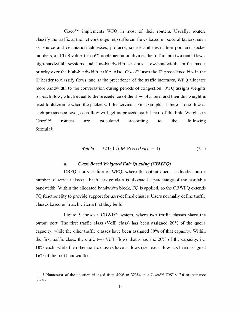
d. Class-Based Weighted Fair Queuing (CBWFQ) CBFQ is a variation of WFQ, where the output queue is divided into a

number of service classes. Each service class is allocated a percentage of the available

bandwidth. Within the allocated bandwidth block, FQ is applied, so the CBWFQ extends

FQ functionality to provide support for user-defined classes. Users normally define traffic

classes based on match criteria that they build.

Figure 5 shows a CBWFQ system, where two traffic classes share the

output port. The first traffic class (VoIP class) has been assigned 20% of the queue

capacity, while the other traffic classes have been assigned 80% of that capacity. Within

the first traffic class, there are two VoIP flows that share the 20% of the capacity, i.e.

10% each, while the other traffic classes have 5 flows (i.e., each flow has been assigned

16% of the port bandwidth).

1 Numerator of the equation changed from 4096 to 32384 in a Cisco™ IOS© v12.0 maintenance

release.

14

SCH

EDU

LER

PORT

VoIP Queu Class (20%)

Other_IP Class (80%)

Two VoIP flows.Each is allocated 1/2of the 20% port BW.

Five Other-IP flows.Each is allocated 1/5of the 80% port BW.

20% of the Port BW

80% of the Port BW

Figure 5. Class-Based Weighted Fair Queuing

Other WFQ variations in addition to the CBWFQ are the Self-clocking

Fair Queuing (SCFQ), Worst-case Fair Weighted Fair Queuing (WF2Q), and Worst-case

Fair Weighted Fair Queuing+ (WF2Q+).

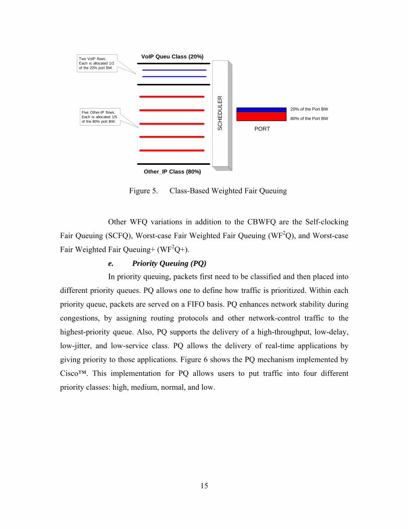
e. Priority Queuing (PQ) In priority queuing, packets first need to be classified and then placed into

different priority queues. PQ allows one to define how traffic is prioritized. Within each

priority queue, packets are served on a FIFO basis. PQ enhances network stability during

congestions, by assigning routing protocols and other network-control traffic to the

highest-priority queue. Also, PQ supports the delivery of a high-throughput, low-delay,

low-jitter, and low-service class. PQ allows the delivery of real-time applications by

giving priority to those applications. Figure 6 shows the PQ mechanism implemented by

Cisco™. This implementation for PQ allows users to put traffic into four different

priority classes: high, medium, normal, and low.

15

Figure 6. Priority Queuing (From Ref. 9)

The PQ algorithm gives higher-priority queues absolute preferential

treatment over the low-priority queues. Priority lists are built by users to set the rules that

describe how packets should be assigned to priority queues. Packets in Cisco™ routers

are classified according to protocol or sub-protocol type, incoming interface, packet size,

fragments, and access lists.

f. Random Early Detection (RED) The integrated services, which also include the congestion avoidance

techniques, anticipate congestions before they occur and try to avoid them. One of the

most popular congestion avoidance techniques is Random Early Detection (RED),

introduced in [17].

The purpose of introducing RED was to overcome a phenomenon termed

global synchronization, which occurred when congestion took place in a network. As a

result, most TCP connections enter the slow-start state (i.e., decreased transmission rate)

at about the same time, and then come out of the slow-start also at about the same time,

which causes the network to be congested another time.

RED takes advantage of the congestion control mechanism of TCP by

dropping random packets to force the source to slow-down transmission. TCP restarts

16

quickly and adapts its transmission speed to the network’s capacity, which descends back

to square one. To force TCP to adapt to network capacity, RED assigns two threshold

values, minimum threshold THmin, and maximum threshold THmax. If the average queue

size exceeds the minimum threshold THmin, RED starts dropping packets. The number of

packets dropped increases linearly as the average queue size increases until it reaches the

maximum threshold THmax. All packets are dropped if the average queue size exceeds the

maximum threshold THmax.

Cisco’s™ implementation of RED is called Weighted Random Early

Detection (WRED) which combines the capabilities of the RED algorithm with IP

precedence to provide preferential service for high-priority traffic. The IP precedence

level is used by WRED to determine when a packet can be dropped. WRED assigns

minimum threshold values THmin according to the precedence level. For example, WRED

may assign for precedence 0 a minimum threshold THmin of 20, and for precedence 1,

THmin of 22. In this case, packets of precedence 0 will be dropped first, because they have

a lower minimum threshold THmin. Figure 7 shows WRED in process.

Figure 7. Weighted Random Early Detection (From Ref. 9)

3. Differentiated Services

The objective of differentiated services (DS) is to provide differing levels of QoS

to different traffic flows. RFC 2474 [18] defines the differentiated services architecture,

17

18

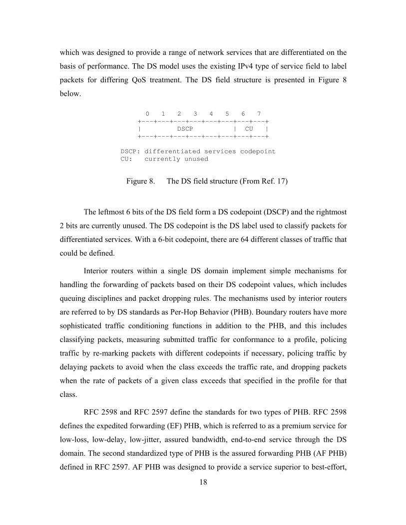
which was designed to provide a range of network services that are differentiated on the

basis of performance. The DS model uses the existing IPv4 type of service field to label

packets for differing QoS treatment. The DS field structure is presented in Figure 8

below.

0 1 2 3 4 5 6 7 +---+---+---+---+---+---+---+---+ | DSCP | CU | +---+---+---+---+---+---+---+---+

DSCP: differentiated services codepoint CU: currently unused

Figure 8. The DS field structure (From Ref. 17)

The leftmost 6 bits of the DS field form a DS codepoint (DSCP) and the rightmost

2 bits are currently unused. The DS codepoint is the DS label used to classify packets for

differentiated services. With a 6-bit codepoint, there are 64 different classes of traffic that

could be defined.

Interior routers within a single DS domain implement simple mechanisms for

handling the forwarding of packets based on their DS codepoint values, which includes

queuing disciplines and packet dropping rules. The mechanisms used by interior routers

are referred to by DS standards as Per-Hop Behavior (PHB). Boundary routers have more

sophisticated traffic conditioning functions in addition to the PHB, and this includes

classifying packets, measuring submitted traffic for conformance to a profile, policing

traffic by re-marking packets with different codepoints if necessary, policing traffic by

delaying packets to avoid when the class exceeds the traffic rate, and dropping packets

when the rate of packets of a given class exceeds that specified in the profile for that

class.

RFC 2598 and RFC 2597 define the standards for two types of PHB. RFC 2598

defines the expedited forwarding (EF) PHB, which is referred to as a premium service for

low-loss, low-delay, low-jitter, assured bandwidth, end-to-end service through the DS

domain. The second standardized type of PHB is the assured forwarding PHB (AF PHB)

defined in RFC 2597. AF PHB was designed to provide a service superior to best-effort,

but at the same time does not require the reservation of resources. Also, it does not

require the differentiation between flows from different users. AF PHB is referred to as

explicit allocation where users can select one class of service from among four classes

defined in the standards, and packets within each class are marked by one of three drop

precedence values. In case of congestion, packets with higher drop precedence values

will be discarded first.

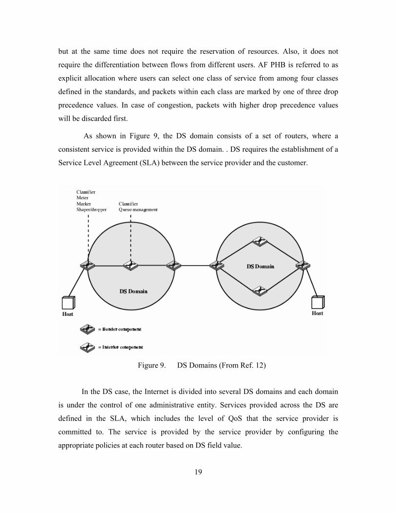
As shown in Figure 9, the DS domain consists of a set of routers, where a

consistent service is provided within the DS domain. . DS requires the establishment of a

Service Level Agreement (SLA) between the service provider and the customer.

Figure 9. DS Domains (From Ref. 12)

In the DS case, the Internet is divided into several DS domains and each domain

is under the control of one administrative entity. Services provided across the DS are

defined in the SLA, which includes the level of QoS that the service provider is

committed to. The service is provided by the service provider by configuring the

appropriate policies at each router based on DS field value.

19

20

C. QOS IMPLEMENTATION IN THE INTEGRATION BETWEEN THE INTERNET AND WIRELESS SENSOR NETWORKS

TCP/IP is widely used in the boundaries of the Internet specifically in the access

and edge networks, and since WSNs are located on the boundaries of the Internet, TCP/IP

is considered to transport the traffic between the two networks. As a result, the

integration module that brings the Internet and wireless sensor networks together will

definitely be based on the existing IP architecture, because this is the common

architecture for both networks. TCP/IP also makes accessing and browsing WSNs easy

and simple. It allows remote browsing using commercial applications, such as Internet

browsers. A TCP\IP-enabled WSN will be accessible from any place on the earth and at

any time.

The Internet is a best-effort network, where delivery of packets is not guaranteed.

IP was not designed to support prioritized traffic or guaranteed performance levels, which

makes it difficult to implement QoS solutions. The only QoS functionality that IP can

support is through the use of the ToS 8 bits. Earlier IPv4 standards defined a 3-bit

precedence field and a 4-bit ToS field, and later this was replaced by the DSPC field

through the differential services standards in RFC 2474 [18].

The traffic of sensor networks is an aggregated packet forwarded by sensor nodes

to the base station (gateway). The traffic of sensor nodes consists mainly of either

periodic measurements (proactive), or driven events based on requests from users on the

Internet (reactive). Some of the packets may carry very high-priority information about

events such as the detection of an intruder in a certain geographical area, which requires

an immediate reaction. Some other packets carry routine or periodic information that

does not require an immediate action. The delay in the high-priority traffic is fatal and

needs to be eliminated or minimized. On the other hand, delays or even drops of routine

traffic can be tolerated to some extent.

As mentioned in Chapter I, the traffic generated by sensor networks has its own

characteristics that distinguish it from the Internet’s traffic. Sensor nodes are required to

work at low data rates according to the 802.15.4 standard. Because of the above reasons,

the data of the sensor networks require special treatment, and some sort of QoS

techniques need to be implemented in the integration link with the Internet. In this thesis,

21

the available QoS techniques used in today’s IP networks will be implemented in the

integration of the Internet and the WSNs for two reasons:

1. To examine the performance of the available QoS techniques when used

in the integration link between WSNs and the Internet.

2. To find out what is required to make those techniques more applicable to

the integration of WSNs with the Internet.

The implementation of available QoS techniques will include using different

queuing disciplines, RSVP, and other policing and shaping techniques. For this purpose

and consistent with the proposed integration model, Cisco™ routers will be used to

provide the required QoS functions on the integration link.

D. SUMMARY QoS is an essential and integral part in computer networking. A new generation of

Internet applications such as VoIP and others require preferential services at routers and

other network components. IP was not built to support QoS, and providing preferential

service is a challenging issue. A Sensor network’s traffic requires special treatment

because it contains time-sensitive and delay-sensitive information. Currently available

QoS techniques are mostly designed to work on the Internet to address issues such as

throughput, delay, and congestion. In the Internet, QoS aims to increase the throughput,

minimize delay, and avoid congestion. The integration of WSNs with the Internet aims

mainly to deliver critical data as fast as possible.

22


23

III. WIRELESS SENSOR NETWORKS OVERVIEW

A. INTRODUCTION The Wireless Sensor Network (WSN) is a network made up of a large number of

tiny, intelligent, and independent sensor nodes. Networking is a key part of what makes

sensor networks work. Networking allows geographical distribution of the sensor nodes.

Unlike their more stable and planned wired counterparts, sensor networks are typically

developed in an ad hoc manner, where unstable links, node failures, and network

interruptions are common. In most cases, sensor networks use wireless communication

between nodes, where each node talks directly to its immediate neighbors within its radio

range. Sensor networks are ad hoc networks, where node layout need not follow any

particular geometry or topology [19].

The IEEE 802.15.4 standard [20] defines both physical and MAC layer protocols

for data communication devices using low data rate, low power and low complexity, and

short-range radio frequency (RF) transmissions in a wireless personal area network

(WPAN). This includes devices such as remote monitoring and control, sensor networks,

smart badges, home automation, and interactive toys. The IEEE 802.15.4 standard was

basically developed after the IEEE 802.15 sub-committee was formed 1998 to develop

WPAN specifications.

ZigBee is an industry consortium that consists of more than fifty companies in

different industrial fields (i.e., semiconductor manufacturers, IP providers, OEMs, etc.)

with the goal of promoting the IEEE 802.15.4 standard. ZigBee ensures interoperability

by defining higher network layers and application interfaces that can be shared among

different manufacturers. This allows devices manufactured by different companies to talk

to one another.

Figure 10 shows the protocol stack for the 802.15.4, which defines the two lower

layers: physical and MAC layers. There is also the ZigBee stack, which defines the

network, security, and application layers. The physical layer (PHY) and media access

control (MAC) layers are specified to work at 868 MHz, 915MHz, and 2.4 GHz

industrial, scientific, and medical (ISM) bands. The air interface for 802.15.4 is direct

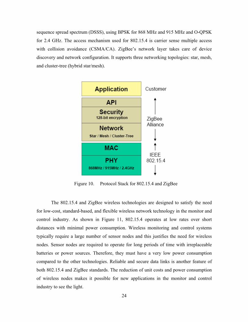
sequence spread spectrum (DSSS), using BPSK for 868 MHz and 915 MHz and O-QPSK

for 2.4 GHz. The access mechanism used for 802.15.4 is carrier sense multiple access

with collision avoidance (CSMA/CA). ZigBee’s network layer takes care of device

discovery and network configuration. It supports three networking topologies: star, mesh,

and cluster-tree (hybrid star/mesh).

Figure 10. Protocol Stack for 802.15.4 and ZigBee

The 802.15.4 and ZigBee wireless technologies are designed to satisfy the need

for low-cost, standard-based, and flexible wireless network technology in the monitor and

control industry. As shown in Figure 11, 802.15.4 operates at low rates over short

distances with minimal power consumption. Wireless monitoring and control systems

typically require a large number of sensor nodes and this justifies the need for wireless

nodes. Sensor nodes are required to operate for long periods of time with irreplaceable

batteries or power sources. Therefore, they must have a very low power consumption

compared to the other technologies. Reliable and secure data links is another feature of

both 802.15.4 and ZigBee standards. The reduction of unit costs and power consumption

of wireless nodes makes it possible for new applications in the monitor and control

industry to see the light.

24

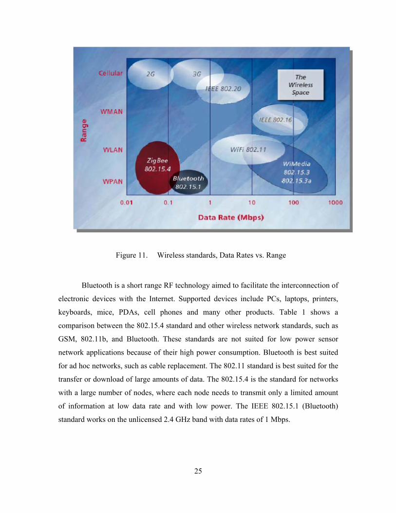
Figure 11. Wireless standards, Data Rates vs. Range

Bluetooth is a short range RF technology aimed to facilitate the interconnection of

electronic devices with the Internet. Supported devices include PCs, laptops, printers,

keyboards, mice, PDAs, cell phones and many other products. Table 1 shows a

comparison between the 802.15.4 standard and other wireless network standards, such as

GSM, 802.11b, and Bluetooth. These standards are not suited for low power sensor

network applications because of their high power consumption. Bluetooth is best suited

for ad hoc networks, such as cable replacement. The 802.11 standard is best suited for the

transfer or download of large amounts of data. The 802.15.4 is the standard for networks

with a large number of nodes, where each node needs to transmit only a limited amount

of information at low data rate and with low power. The IEEE 802.15.1 (Bluetooth)

standard works on the unlicensed 2.4 GHz band with data rates of 1 Mbps.

25

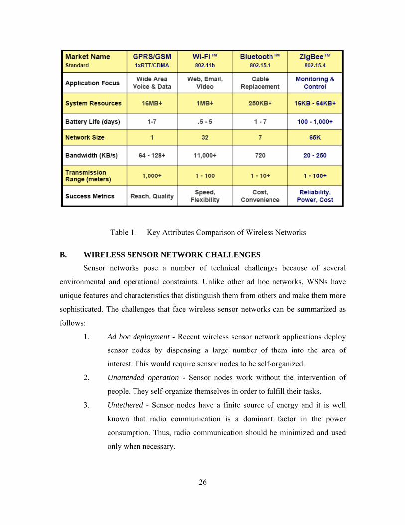
Table 1. Key Attributes Comparison of Wireless Networks

B. WIRELESS SENSOR NETWORK CHALLENGES Sensor networks pose a number of technical challenges because of several

environmental and operational constraints. Unlike other ad hoc networks, WSNs have

unique features and characteristics that distinguish them from others and make them more

sophisticated. The challenges that face wireless sensor networks can be summarized as

follows:

1. Ad hoc deployment - Recent wireless sensor network applications deploy

sensor nodes by dispensing a large number of them into the area of

interest. This would require sensor nodes to be self-organized.

2. Unattended operation - Sensor nodes work without the intervention of

people. They self-organize themselves in order to fulfill their tasks.

3. Untethered - Sensor nodes have a finite source of energy and it is well

known that radio communication is a dominant factor in the power

consumption. Thus, radio communication should be minimized and used

only when necessary.

26

27

4. Dynamic changes - In a WSN environment, changes happen very often

and this includes changes in topology, failure of other nodes, and many

others changes.

5. Communication - Bandwidth is limited which constrains the inter-sensor

communication.

6. Limited computation - WSNs cannot run complicated protocols, because

of the computational power limitation.

7. Sensors may not have global identification because of the large overhead.

8. Fault-tolerant - Sensor nodes are often susceptible to failures due to

power shortages. Therefore, sensor nodes should be fault-tolerant and not

affected by nodes failures.

9. Transmission Media – The wireless transmission channel is subject to

traditional propagation problems, such as fading and attenuation. This

affects the design and selection of the media access control.

10. Quality of service - Some applications are delay-sensitive and time-

sensitive, and intolerant to any delays in the data delivery.

Because of these unique features of WSNs, the focus was to extend the system

lifetime and increase the system robustness. For wired and other wireless networks, the

ultimate objective is to increase the throughput [21]. WSNs differ from traditional

wireless network and from mobile ad hoc networks (MANETs) in several ways. WSNs

have a severe power constrain, and unlike traditional networks, power consumption

levels are critical and decisive. WSNs are generally stationary, except for few mobile

nodes, after the deployment. The data rate of WSNs is very low, compared to traditional

wired networks and other wireless technologies such as the IEEE 802.11.

C. WIRELESS SENSOR NETWORKS REQUIREMENTS In order for the WSN to work properly and efficiently, the following requirements

are needed [22]:

1. Large number of sensors - To cover the target area efficiently, usually a

large number of sensor nodes are used.

2. Low energy consumption - The life of the battery determines the life of the

sensor network.

28

3. Efficient use of the small memory - Routing protocols and tables and other

management protocols should be designed with memory constrained in

mind.

4. Data aggregation - Redundant data from different sensor nodes is

common in WSNs. So, there is a need to aggregate data before sending it

back to data collection centers.

5. Self-organization - Sensor nodes have the ability to organize themselves in

a hierarchical structure and be able to continue working even if one or

more nodes fail.

6. Collaborative signal processing - The objective of WSNs is to detect

events and estimate some measurements, and this requires collaborative

processing power of more than one sensor node.

7. Querying ability - Queries may be sent to a specific region (data-centric)

in the WSN or to an individual sensor node (address-centric).

8. Position awareness - Sensor nodes are required to know their locations,

because data collection is based on the location. It is preferable to have a

GPS-free solution, were locations are estimated based on other affordable

parameters.

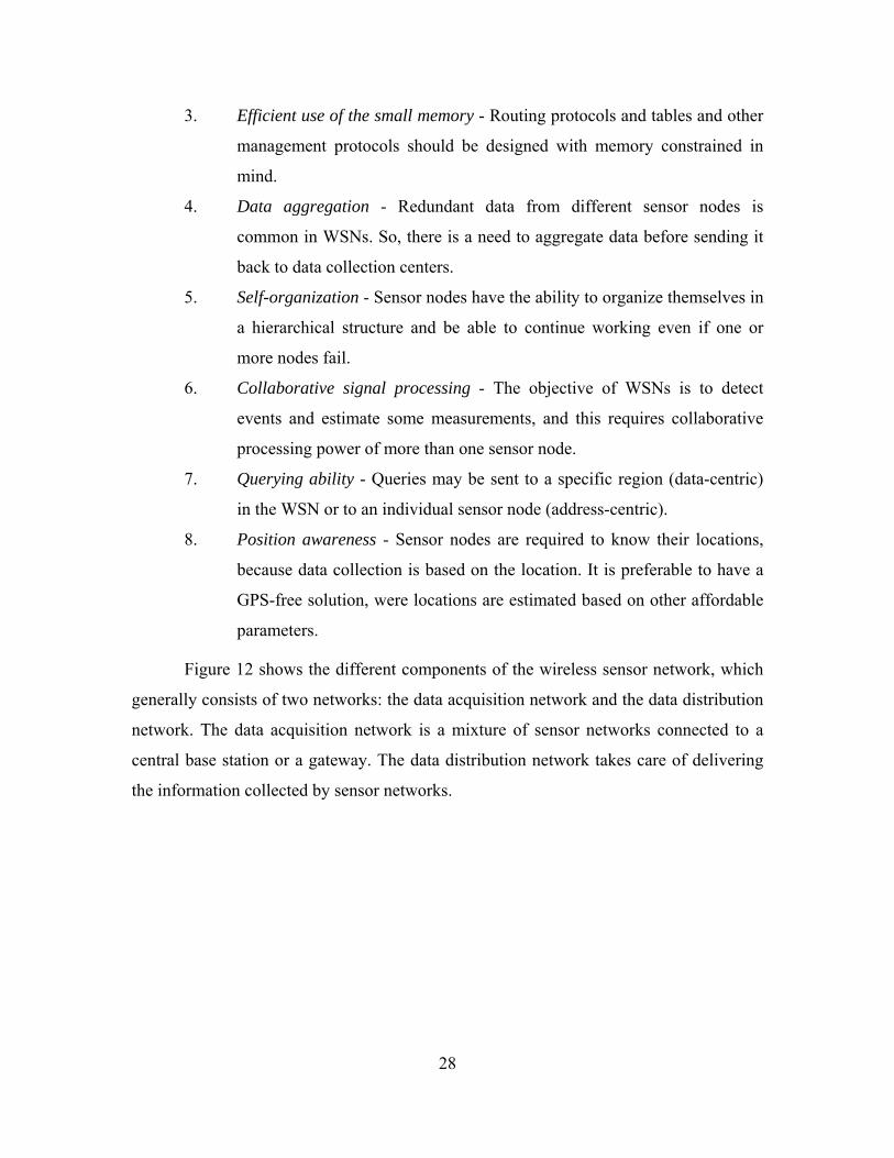
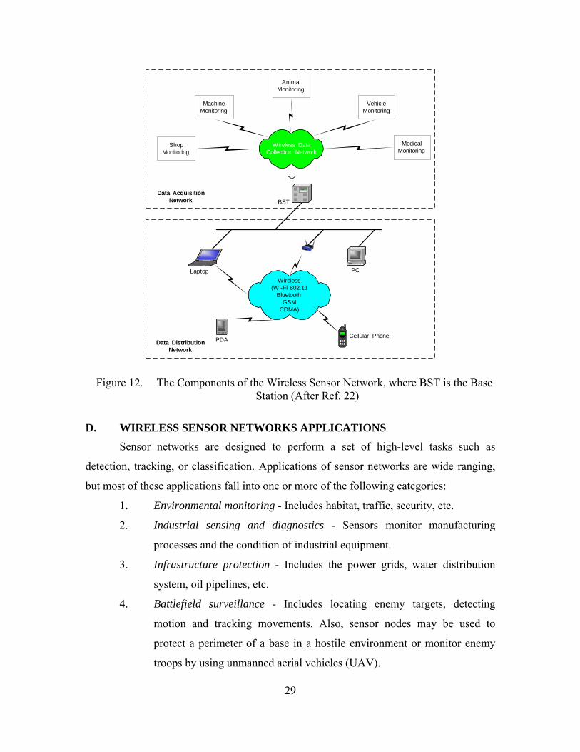
Figure 12 shows the different components of the wireless sensor network, which

generally consists of two networks: the data acquisition network and the data distribution

network. The data acquisition network is a mixture of sensor networks connected to a

central base station or a gateway. The data distribution network takes care of delivering

the information collected by sensor networks.

MedicalMonitoring

VehicleMonitoring

AnimalMonitoring

MachineMonitoring

ShopMonitoring

Wireless DataCollection Network

BST

Wireless(Wi-Fi 802.11

BluetoothGSM

CDMA)

PC

PDA

Laptop

Cellular Phone

Data AcquisitionNetwork

Data DistributionNetwork

Figure 12. The Components of the Wireless Sensor Network, where BST is the Base

Station (After Ref. 22)

D. WIRELESS SENSOR NETWORKS APPLICATIONS Sensor networks are designed to perform a set of high-level tasks such as

detection, tracking, or classification. Applications of sensor networks are wide ranging,

but most of these applications fall into one or more of the following categories:

1. Environmental monitoring - Includes habitat, traffic, security, etc.

2. Industrial sensing and diagnostics - Sensors monitor manufacturing

processes and the condition of industrial equipment.

3. Infrastructure protection - Includes the power grids, water distribution

system, oil pipelines, etc.

4. Battlefield surveillance - Includes locating enemy targets, detecting

motion and tracking movements. Also, sensor nodes may be used to

protect a perimeter of a base in a hostile environment or monitor enemy

troops by using unmanned aerial vehicles (UAV).

29

30

5. Medical diagnostics and health care - Sensors can help monitor the vital

signs of patients and remotely connect doctors’ offices with patients.

6. Urban terrain mapping.

7. Asset and warehouse management - Sensors are used for tracking assets,

such as vehicles and trucks or goods by using either GPS-equipped

locators or radio frequency identification (RFID) tags. With the wide

adoption of RFIDs, warehouses and department stores are able to collect

real-time inventory and retail information.

8. Automotive - Dedicated short-range communication (DSRC) will allow

vehicle-to-vehicle communications. Thus, cars soon will be able to talk to

each other and to the roadside infrastructure in order o provide more safety

on the roads.

E. WIRELESS SENSOR NETWORKS ROUTING TECHNIQUES

Unlike conventional networks, WSNs are energy limited with irreplaceable

energy sources that make the use of the same traditional routing techniques irrelevant.

Routing in sensor networks is very challenging due to the inherited features of sensor

networks. The deployment of a numerous number of sensor nodes makes it impossible to

build a global addressing scheme. Therefore, classical IP-based protocols are inapplicable

to sensor networks. The most appropriate protocols are those that discover routes using

local, lightweight, scalable techniques, while avoiding using lengthy routing tables and

expensive link state advertisements’ overhead.

Wireless routing protocols are basically designed for mobile ad hoc wireless

networks, but they are also applicable for sensor networks with some exceptions, because

most of them are energy-aware protocols. In this section, only applicable protocols to

wireless sensor networks will be discussed. Conventional routing protocols, which were

designed mainly for IP-based networks, cannot be used directly in a WSN for the

following reasons [23]:

1. WSNs are randomly deployed in inaccessible terrain or disaster relief

operations, which implies that WSNs perform sensing and communication

with no human intervention. Therefore, WSNs should be self-organized.

31

2. The design requirements of WSNs change with application, i.e., each

application has specific requirements such as latency, precision, etc.

3. Data redundancy in WSNs occurs due to the fact that many sensors are

located very close to each other.

4. WSNs are data-centric networks, i.e., data are requested based on certain

attributes.

5. In data-centric networks, it is not necessary to request an individual

sensor. Instead, requests are forwarded to any sensor with similar

capabilities.

6. Due to the large number of deployed sensors and expensive overhead,

conventional address-centric schemes will not work. Thus, WSNs use an

attribute-based addressing scheme. For example, if the query is

temperature >30 º C, then only sensor nodes that sense temperature >30 º C

should reply to the query.

7. Because data collection is based on the sensor node location, position

awareness is important.

8. Almost all applications of WSNs require the flow of sensed data from

multiple regions to a particular node (sink).

For WSNs, routing protocols are required to take into consideration all the

mentioned challenges and perform routing tasks with minimum energy consumption.

F. SENSOR NETWORK PLATFORMS

1. Sensor Node Hardware Sensor node hardware can be grouped into three categories, each of which entails

a different set of trade-offs in the design choice.

1. Augmented general-purpose computers: Examples in this category include

low power PC’s, embedded PCs, custom designed PCs, and PDAs. These

platforms run either off-the-shelf operating systems such as Windows®

CE, Linux, or real-time operating systems. Most the platforms under this

category use standard wireless communication protocols such as Bluetooth

and IEEE 802.11. Devices in this category are more complicated and

power hungry compared to dedicated sensor nodes.

32

2. Dedicated embedded sensor nodes: Examples include the Berkeley mote

family [24], the UCLA Medusa family [25], Ember nodes, and MIT

µAMP [26]. These platforms use commercial off-the-shelf (COTS) chip

sets with an emphasis on small form factor, low power processing and

communication, and simple interfaces. Nodes in this category support at

least one operating system, such as TinyOS, with its companion

programming language, nesC.

3. System-on-chip (SoC): Examples in this category include smart dust [27],

the BWRC picoradio node [28], and the PASTA node [29] These

technologies integrate CMOS, MEMS, and RF technologies to build

extremely low power and small footprint sensor nodes, with sensing,

computation, and communication capabilities.

The Berkeley motes have gained wide popularity because of their small form

factor, open source software development, and commercial availability. The typical

Berkeley MICA mote, as shown in Figure 13, has a two-CPU design. The main

microcontroller (MCU) takes care of the regular processing. A separate and less capable

coprocessor is only active when the MCU is being reprogrammed. The small memory

sizes introduced great challenges to mote programmers who are required to keep the code

footprint very small. The RF transceiver on MICA motes operates on the 916 MHz band,

and achieves a data bit rate of 50 Kbps. All Berkeley MICA motes support a 51 pin I/O

connector that is used to connect sensors, actuators, serial boards, or parallel boards.

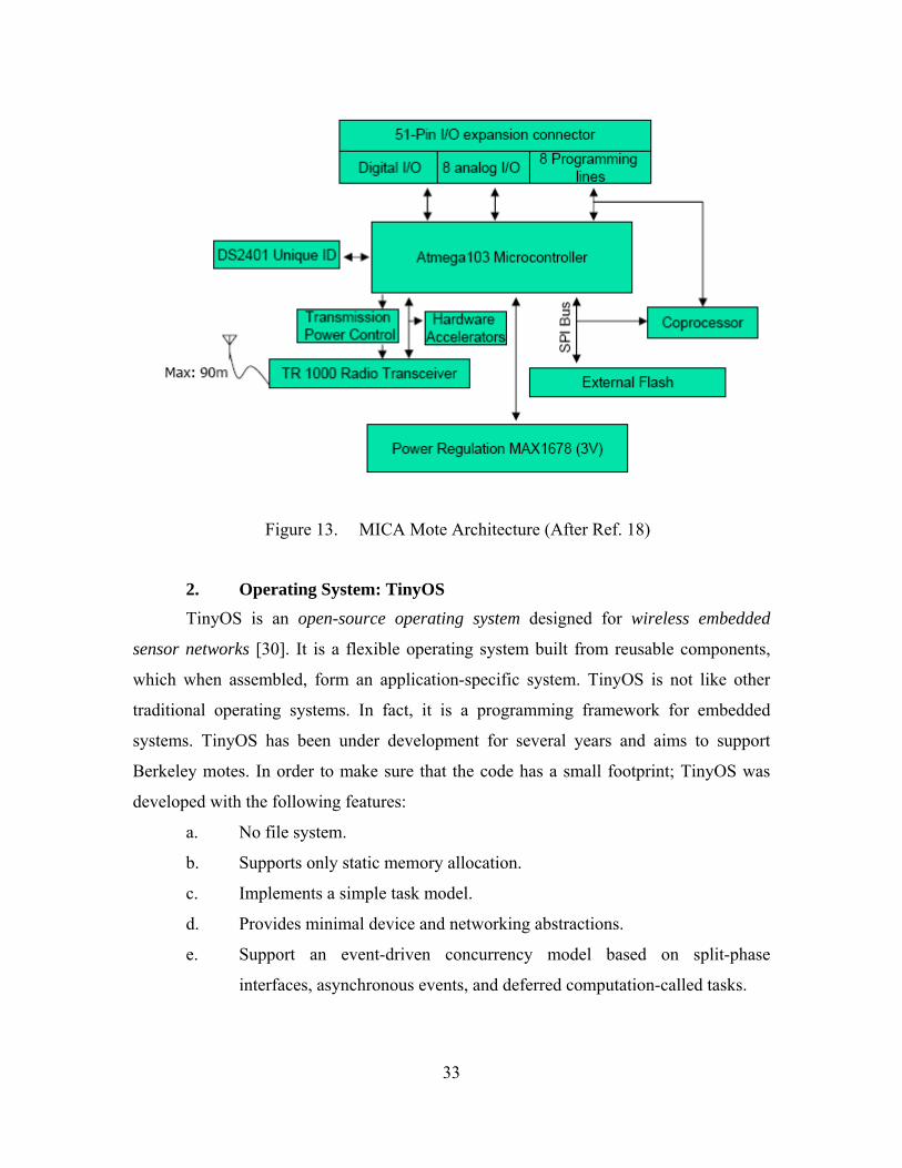
Figure 13. MICA Mote Architecture (After Ref. 18)

2. Operating System: TinyOS TinyOS is an open-source operating system designed for wireless embedded

sensor networks [30]. It is a flexible operating system built from reusable components,

which when assembled, form an application-specific system. TinyOS is not like other

traditional operating systems. In fact, it is a programming framework for embedded

systems. TinyOS has been under development for several years and aims to support

Berkeley motes. In order to make sure that the code has a small footprint; TinyOS was

developed with the following features:

a. No file system.

b. Supports only static memory allocation.

c. Implements a simple task model.

d. Provides minimal device and networking abstractions.

e. Support an event-driven concurrency model based on split-phase

interfaces, asynchronous events, and deferred computation-called tasks.

33

34

Any TinyOS program is, in fact, a graph of components, each of which is an

independent computational entity that exposes one or more interfaces. These components

have three computational abstractions: commands, events, and tasks. Commands and

events are mechanisms for inter-component communication, while tasks are used to

express intra-component concurrency.

TinyDB [31] is a declarative query processor built on TinyOS, which allows users

to interact with a network through a high-level interface. In TinyOS, queries propagate

through the network and perform both data collection and in-network aggregation. The

in-network aggregation helps reduce the network bandwidth requirements. The queries

declare the type of data that the user is interested in without any other bandwidth-

consuming details.

G. SUMMARY Wireless sensor networks (WSNs) are expected to be used in a new class of

distributed monitoring applications due to the recent advances in technology. Information

processing in sensor networks is the central theme that brings all the components together

in order to achieve the overall system goal. New ways are required to network, organize,

query, and program the ubiquitous sensors, actuators, and embedded processing. Energy

constraints on sensor nodes are still the main challenge for developers, users, and

manufacturers. More efficient energy-aware communication algorithms need to be

developed. As technology advances, both the size and cost of sensor nodes will be

reduced significantly, which will allow for the spread of new distributed and ubiquitous

applications.

35

IV. INTEGRATION ARCHITECTURE

A. INTRODUCTION Data collected by sensor networks are required to be transmitted promptly to users

of the Internet for analysis and intelligence gathering. Typically, self-organized sensor

nodes are randomly scattered over the area of interest. Depending on the communication

schemes used in deployed WSNs, collected data are propagated back to a central node

called a sink or gateway. The gateway is a more complicated sensor node that has

sufficient capabilities to query and communicate with other sensor nodes within the

coverage area. Typically, the gateway is connected to an enterprise network or to the

Internet in order to send/receive data to/from deployed WSNs. The connection between

the gateway and the Internet is either a wired or wireless link, depending on the

deployment environment. For example, if sensor nodes were deployed in a hostile

environment, then the use of a wired link could be difficult or even impossible. So, the

integration link between the Internet and the WSNs could be a satellite link, IEEE

802.11, or just a dedicated radio packet link.

B. PROPOSED INTEGRATION MODULE OVERVIEW This thesis introduces an integration module for the wireless sensor networks and

the Internet. Figure 14 shows the architecture of the proposed integration module. The

proposed integration module aims to facilitate the flow of packets between the two

domains (i.e., the Internet and WSNs) through the implementation of a set of QoS

techniques, and allows the implementation of QoS to be continuous, dynamic, and self-

adaptive. The proposed integration module has the following objectives:

1. Making the traffic flow smoothly and promptly.

2. Making the traffic less susceptible to delays and congestions.

3. Providing security and reliability through the implementation of the

wireless sensor networks registration protocol (WSNRP).

4. Reducing the setup time of the integration link.

5. Self-adapting QoS functions to match changes on traffic patterns.

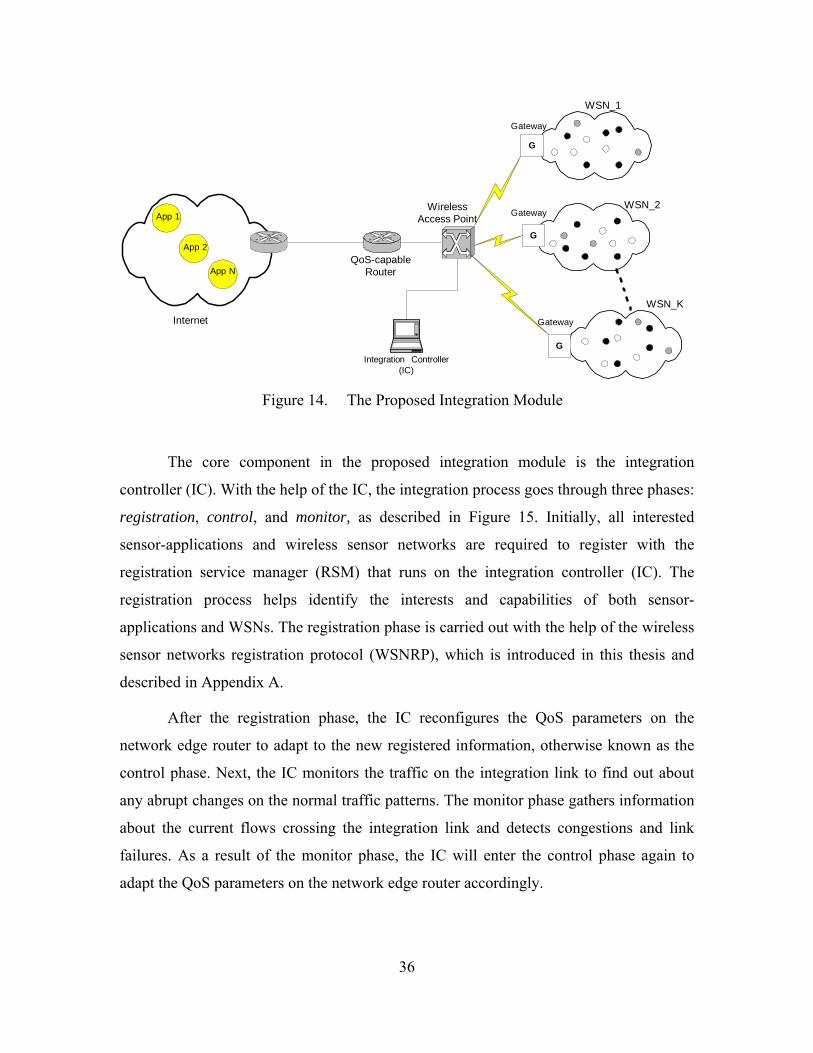
G

G

G

App 1

Internet

WirelessAccess Point

WSN_1

WSN_2

WSN_K

Gateway

Gateway

Gateway

QoS-capableRouter

Integration Controller(IC)

App 2

App N

Figure 14. The Proposed Integration Module

The core component in the proposed integration module is the integration

controller (IC). With the help of the IC, the integration process goes through three phases:

registration, control, and monitor, as described in Figure 15. Initially, all interested

sensor-applications and wireless sensor networks are required to register with the

registration service manager (RSM) that runs on the integration controller (IC). The

registration process helps identify the interests and capabilities of both sensor-

applications and WSNs. The registration phase is carried out with the help of the wireless

sensor networks registration protocol (WSNRP), which is introduced in this thesis and

described in Appendix A.

After the registration phase, the IC reconfigures the QoS parameters on the

network edge router to adapt to the new registered information, otherwise known as the

control phase. Next, the IC monitors the traffic on the integration link to find out about

any abrupt changes on the normal traffic patterns. The monitor phase gathers information

about the current flows crossing the integration link and detects congestions and link

failures. As a result of the monitor phase, the IC will enter the control phase again to

adapt the QoS parameters on the network edge router accordingly.

36

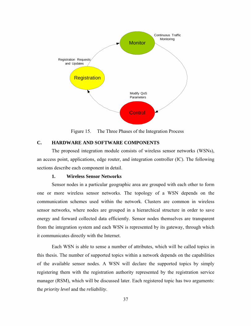
Registration

Control

Monitor

Registration Requestsand Updates

Modify QoSParameters

Continuous TrafficMonitoring

Figure 15. The Three Phases of the Integration Process

C. HARDWARE AND SOFTWARE COMPONENTS

The proposed integration module consists of wireless sensor networks (WSNs),

an access point, applications, edge router, and integration controller (IC). The following

sections describe each component in detail.

1. Wireless Sensor Networks Sensor nodes in a particular geographic area are grouped with each other to form

one or more wireless sensor networks. The topology of a WSN depends on the

communication schemes used within the network. Clusters are common in wireless

sensor networks, where nodes are grouped in a hierarchical structure in order to save

energy and forward collected data efficiently. Sensor nodes themselves are transparent

from the integration system and each WSN is represented by its gateway, through which

it communicates directly with the Internet.

Each WSN is able to sense a number of attributes, which will be called topics in

this thesis. The number of supported topics within a network depends on the capabilities

of the available sensor nodes. A WSN will declare the supported topics by simply

registering them with the registration authority represented by the registration service

manager (RSM), which will be discussed later. Each registered topic has two arguments:

the priority level and the reliability.

37

38

The priority level of a certain topic tells how urgent the data of that topic within a

certain network is, while the reliability argument tells how reliable the data collected for

that topic on a certain network are. The priority information associated with a topic

during a communication session will be used to determine the link resources, such as

bandwidth.

The reliability information associated with each topic is crucial to the applications

on the Internet. An application on the Internet uses the reliability information to filter out

the data that do not satisfy the reliability requirements of that application.

Gateway nodes in sensor networks are very important elements. They provide the

ability to establish long-range communication in order to deliver critical information to

remote locations. The gateway is an application layer device that has the capabilities to

respond to certain types of requests and tasks

2. Access Point

To have a multiple WSNs connected to the Internet, an access point with multi-

access wireless capabilities is required. The access point has a wireless interface with the

WSNs from one side and a wired interface with the Internet from the other side. The

wireless interface between the access point and a WSN is a multiple access wireless

technology such as the IEEE 802.11. Throughout the experimental phase of this thesis,

several wired interfaces were used. Ethernet, Fast Ethernet, and variable-speed serial

connections were among the technologies that were implemented between the access

point and the Internet.

3. Applications Users on the Internet run applications that query the WSNs. Applications on the

Internet receive the collected data from WSNs for analysis and intelligence gathering.

Throughout this thesis, the term sensor-application will be used to describe those

applications running on the Internet and interested in the WSNs. Sensor-applications

could run on different hosts and one host could have more than one sensor-application. It

is assumed that there is an unlimited number of sensor-applications on the Internet, which

initially have no previous knowledge of the available WSNs. So, when a sensor-

application first starts up, it sends a registration request to the registration service

manager (RSM) in order to receive a list of valid WSN candidates.

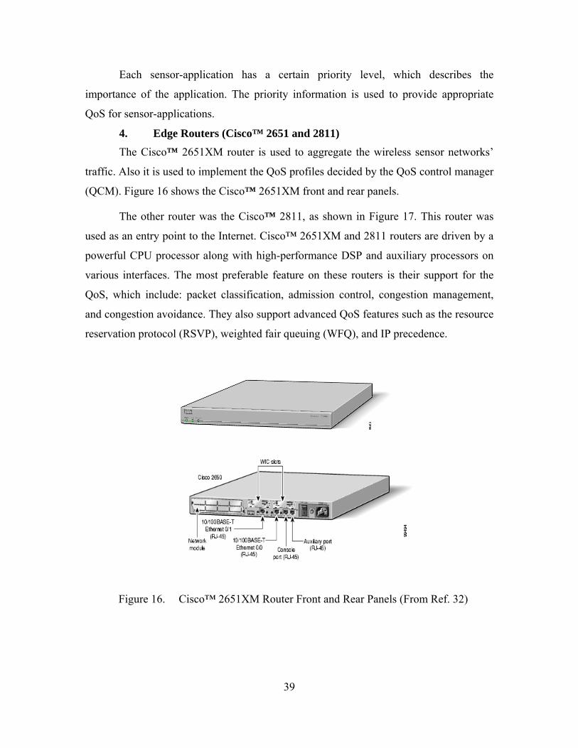
Each sensor-application has a certain priority level, which describes the

importance of the application. The priority information is used to provide appropriate

QoS for sensor-applications.

4. Edge Routers (Cisco™ 2651 and 2811) The Cisco™ 2651XM router is used to aggregate the wireless sensor networks’

traffic. Also it is used to implement the QoS profiles decided by the QoS control manager

(QCM). Figure 16 shows the Cisco™ 2651XM front and rear panels.

The other router was the Cisco™ 2811, as shown in Figure 17. This router was

used as an entry point to the Internet. Cisco™ 2651XM and 2811 routers are driven by a

powerful CPU processor along with high-performance DSP and auxiliary processors on

various interfaces. The most preferable feature on these routers is their support for the

QoS, which include: packet classification, admission control, congestion management,

and congestion avoidance. They also support advanced QoS features such as the resource

reservation protocol (RSVP), weighted fair queuing (WFQ), and IP precedence.

Figure 16. Cisco™ 2651XM Router Front and Rear Panels (From Ref. 32)

39

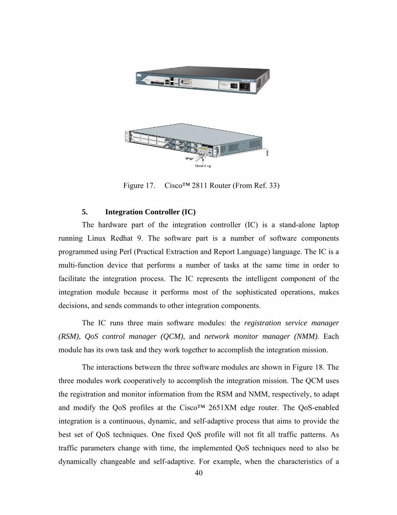
Figure 17. Cisco™ 2811 Router (From Ref. 33)

5. Integration Controller (IC) The hardware part of the integration controller (IC) is a stand-alone laptop

running Linux Redhat 9. The software part is a number of software components

programmed using Perl (Practical Extraction and Report Language) language. The IC is a

multi-function device that performs a number of tasks at the same time in order to

facilitate the integration process. The IC represents the intelligent component of the

integration module because it performs most of the sophisticated operations, makes

decisions, and sends commands to other integration components.

The IC runs three main software modules: the registration service manager

(RSM), QoS control manager (QCM), and network monitor manager (NMM). Each

module has its own task and they work together to accomplish the integration mission.

The interactions between the three software modules are shown in Figure 18. The

three modules work cooperatively to accomplish the integration mission. The QCM uses

the registration and monitor information from the RSM and NMM, respectively, to adapt

and modify the QoS profiles at the Cisco™ 2651XM edge router. The QoS-enabled

integration is a continuous, dynamic, and self-adaptive process that aims to provide the

best set of QoS techniques. One fixed QoS profile will not fit all traffic patterns. As

traffic parameters change with time, the implemented QoS techniques need to also be

dynamically changeable and self-adaptive. For example, when the characteristics of a 40

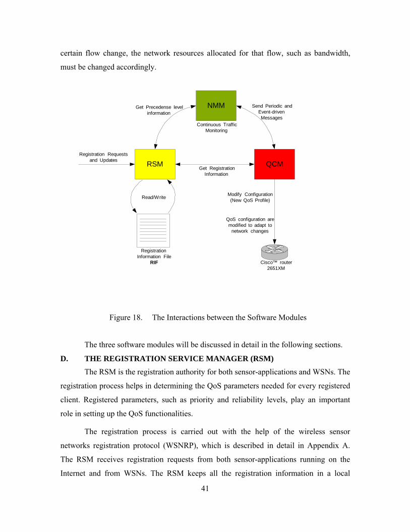
certain flow change, the network resources allocated for that flow, such as bandwidth,

must be changed accordingly.

RegistrationInformation File

RIF

Registration Requestsand Updates

Read/Write Modify Configuration(New QoS Profile)

Get RegistrationInformation

Continuous TrafficMonitoring

Send Periodic andEvent-drivenMessages

QoS configuration aremodified to adapt to

network changes

Cisco™ router2651XM

NMM

QCMRSM

Get Precedense levelinformation

Figure 18. The Interactions between the Software Modules

The three software modules will be discussed in detail in the following sections.

D. THE REGISTRATION SERVICE MANAGER (RSM) The RSM is the registration authority for both sensor-applications and WSNs. The

registration process helps in determining the QoS parameters needed for every registered

client. Registered parameters, such as priority and reliability levels, play an important

role in setting up the QoS functionalities.

The registration process is carried out with the help of the wireless sensor

networks registration protocol (WSNRP), which is described in detail in Appendix A.

The RSM receives registration requests from both sensor-applications running on the

Internet and from WSNs. The RSM keeps all the registration information in a local

41

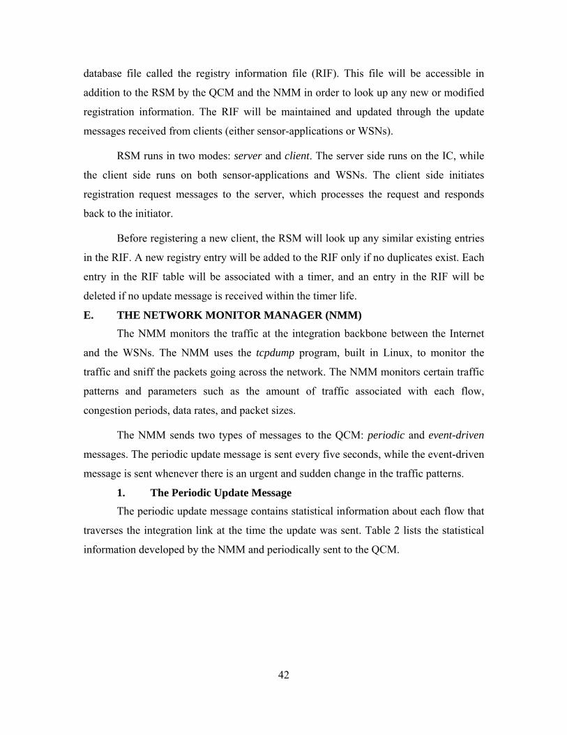
42

database file called the registry information file (RIF). This file will be accessible in

addition to the RSM by the QCM and the NMM in order to look up any new or modified

registration information. The RIF will be maintained and updated through the update

messages received from clients (either sensor-applications or WSNs).

RSM runs in two modes: server and client. The server side runs on the IC, while

the client side runs on both sensor-applications and WSNs. The client side initiates

registration request messages to the server, which processes the request and responds

back to the initiator.

Before registering a new client, the RSM will look up any similar existing entries

in the RIF. A new registry entry will be added to the RIF only if no duplicates exist. Each

entry in the RIF table will be associated with a timer, and an entry in the RIF will be

deleted if no update message is received within the timer life.

E. THE NETWORK MONITOR MANAGER (NMM)

The NMM monitors the traffic at the integration backbone between the Internet

and the WSNs. The NMM uses the tcpdump program, built in Linux, to monitor the

traffic and sniff the packets going across the network. The NMM monitors certain traffic

patterns and parameters such as the amount of traffic associated with each flow,

congestion periods, data rates, and packet sizes.

The NMM sends two types of messages to the QCM: periodic and event-driven

messages. The periodic update message is sent every five seconds, while the event-driven

message is sent whenever there is an urgent and sudden change in the traffic patterns.

1. The Periodic Update Message The periodic update message contains statistical information about each flow that

traverses the integration link at the time the update was sent. Table 2 lists the statistical

information developed by the NMM and periodically sent to the QCM.

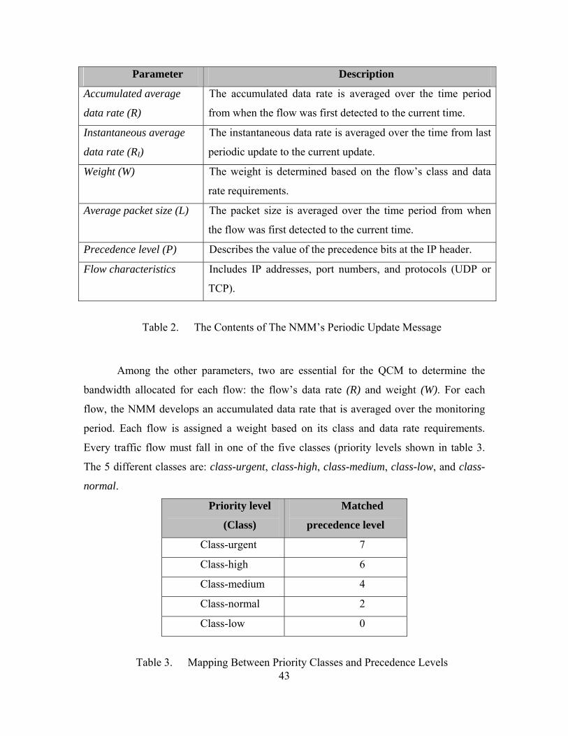
43

Parameter Description

Accumulated average

data rate (R)

The accumulated data rate is averaged over the time period

from when the flow was first detected to the current time.

Instantaneous average

data rate (RI)

The instantaneous data rate is averaged over the time from last

periodic update to the current update.

Weight (W) The weight is determined based on the flow’s class and data

rate requirements.

Average packet size (L) The packet size is averaged over the time period from when

the flow was first detected to the current time.

Precedence level (P) Describes the value of the precedence bits at the IP header.

Flow characteristics Includes IP addresses, port numbers, and protocols (UDP or

TCP).

Table 2. The Contents of The NMM’s Periodic Update Message

Among the other parameters, two are essential for the QCM to determine the

bandwidth allocated for each flow: the flow’s data rate (R) and weight (W). For each

flow, the NMM develops an accumulated data rate that is averaged over the monitoring

period. Each flow is assigned a weight based on its class and data rate requirements.

Every traffic flow must fall in one of the five classes (priority levels shown in table 3.

The 5 different classes are: class-urgent, class-high, class-medium, class-low, and class-

normal.

Priority level

(Class)

Matched

precedence level

Class-urgent 7

Class-high 6

Class-medium 4

Class-normal 2

Class-low 0

Table 3. Mapping Between Priority Classes and Precedence Levels

Each flow that belongs to class-urgent is assigned a weight of 7 no matter how

many flows there are. For example, if there are two urgent flows, then each flow is

assigned a weight of 7. The first flow with the highest data rate and belongs to class-high

is assigned a weight of 6, and the next flow with the second highest data rate is assigned a

weight of 5, and so on. The same applies to class-medium and class-normal with the

exception that weighting starts with 4 for class-medium and with 2 for class-normal.

Table 4 shows the weights assignments for flows that belong to different classes.

Class Weights

Data rate decreases in this direction

1st flow 2nd flow 3rd flow 4th flow 5th flow 6th flow Others

Urgent 7 7 7 7 7 7 7

High 6 5 4 3 2 1 0

Medium 4 3 2 1 0 0 0

Normal 2 1 0 0 0 0 0

Low 0 0 0 0 0 0 0

Table 4. Weights Assignment Based on Flow’s Class and Data Rate

Compared to the weighting scheme used by Cisco routers to allocate bandwidth in

fair queuing systems, this weighting scheme allocates more bandwidth to urgent and high

class traffic than medium and low class traffic. In Cisco’s flow weighting scheme for

WFQ described in [10], each flow will get precedence + 1 parts of the link. For example,

if you have 18 precedence 1 flows and one precedence 7 flow, then each flow with

precedence 1 will be allocated 2 /(8 2(18)) 2 / 44+ = , i.e., the 18 precedence 1 flows will

be allocated 36/44 ( 82%) of the link bandwidth, while the precedence 7 flow is allocated

just 8/44 (18%). If the precedence 7 flow is a video flow with 768 Kbps data rate, then it

will be allocated only 277Kbps bandwidth. So, Cisco’s implementation of WFQ does not

take into consideration the data rate requirements of each flow.

44

45

The weighting scheme described in Table 4, along with the bandwidth allocation

algorithm (BAA) described in the following sections, are used to determine the

bandwidth allocated for each flow. The proposed integration module takes into

consideration both the precedence level and the data rate when allocating bandwidth for

each flow in the queuing system.

2. The Event-driven Message An alert message is sent to the QCM whenever the NMM detects certain events

such as congestion periods and failure of the router’s interface. Congestion periods are

detected by monitoring the number of dropped packets by the router. If a flow exceeds

the maximum allocated queue length, the router will start to drop packets from that

flow’s queue. The queue lengths in Cisco routers are configurable and have maximum

limits. Also, whenever the interface that connects the edge router to the Internet goes

down, the NMM sends an alert massage to the QCM.

F. QOS CONTROL MANAGER (QCM) The QCM determines the best QoS profiles that must be used by the edge router

based on the feedback information from both the RSM and NMM. All the configuration

commands are sent to the edge router through a telnet session that is carried out with the

help of two Perl libraries called Net::Telnet [34] and Net::Telnet::Cisco [35].

QoS profiles mainly consist of queuing disciplines, traffic policing and shaping.

Because of their superior performance over other queuing disciplines, both priority

queuing (PQ) and class-based weighted fair queuing (CBWFQ) were selected as the

queuing systems at the edge router.

Along with other queuing disciplines, PQ and CBWFQ were tested in a 108%

overloaded UDP network at different data rates. PQ and CBWFQ outperformed other

queuing systems such as the weighted fair queuing (WFQ) and custom queuing (CQ).

Figures 19 and 20 show the results of the test. Figure 19 shows the delay exercised by

traffic utilizing different queuing systems. Figure 20 shows the number of dropped

packets for the same traffic and under the same conditions.

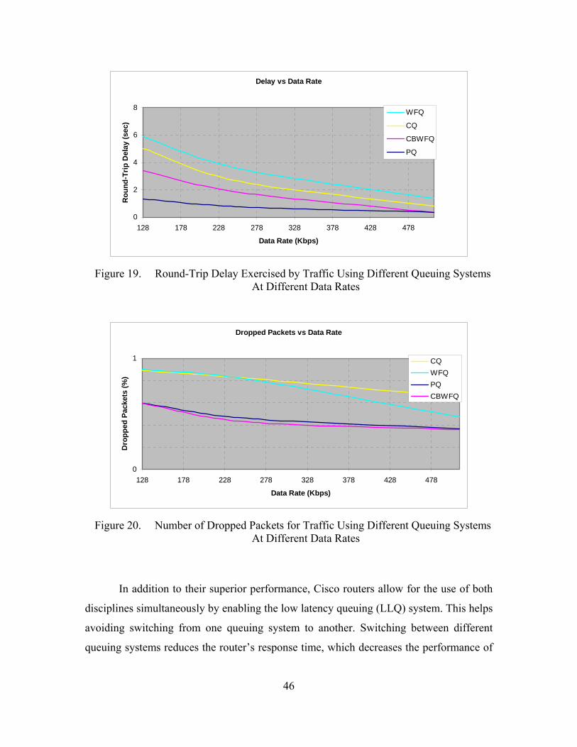
Delay vs Data Rate

0

2

4

6

8

128 178 228 278 328 378 428 478

Data Rate (Kbps)

Rou

nd-T

rip D

elay

(sec

)WFQ

CQ

CBWFQ

PQ

Figure 19. Round-Trip Delay Exercised by Traffic Using Different Queuing Systems

At Different Data Rates

Dropped Packets vs Data Rate

0

1

128 178 228 278 328 378 428 478

Data Rate (Kbps)

Dro

pped

Pac

kets

(%)

CQWFQPQCBWFQ

Figure 20. Number of Dropped Packets for Traffic Using Different Queuing Systems

At Different Data Rates

In addition to their superior performance, Cisco routers allow for the use of both

disciplines simultaneously by enabling the low latency queuing (LLQ) system. This helps

avoiding switching from one queuing system to another. Switching between different

queuing systems reduces the router’s response time, which decreases the performance of

46

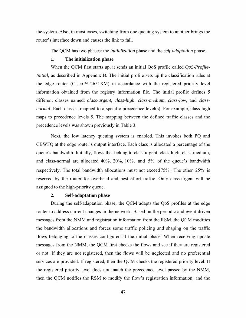
the system. Also, in most cases, switching from one queuing system to another brings the

router’s interface down and causes the link to fail.

The QCM has two phases: the initialization phase and the self-adaptation phase.

1. The initialization phase When the QCM first starts up, it sends an initial QoS profile called QoS-Profile-

Initial, as described in Appendix B. The initial profile sets up the classification rules at

the edge router (Cisco™ 2651XM) in accordance with the registered priority level

information obtained from the registry information file. The initial profile defines 5

different classes named: class-urgent, class-high, class-medium, class-low, and class-

normal. Each class is mapped to a specific precedence level(s). For example, class-high

maps to precedence levels 5. The mapping between the defined traffic classes and the

precedence levels was shown previously in Table 3.

Next, the low latency queuing system is enabled. This invokes both PQ and

CBWFQ at the edge router’s output interface. Each class is allocated a percentage of the

queue’s bandwidth. Initially, flows that belong to class-urgent, class-high, class-medium,

and class-normal are allocated and 5% of the queue’s bandwidth

respectively. The total bandwidth allocations must not exceed . The other is

reserved by the router for overhead and best effort traffic. Only class-urgent will be

assigned to the high-priority queue.

40%, 20%, 10%,

75% 25%

2. Self-adaptation phase During the self-adaptation phase, the QCM adapts the QoS profiles at the edge

router to address current changes in the network. Based on the periodic and event-driven

messages from the NMM and registration information from the RSM, the QCM modifies

the bandwidth allocations and forces some traffic policing and shaping on the traffic

flows belonging to the classes configured at the initial phase. When receiving update

messages from the NMM, the QCM first checks the flows and see if they are registered

or not. If they are not registered, then the flows will be neglected and no preferential

services are provided. If registered, then the QCM checks the registered priority level. If

the registered priority level does not match the precedence level passed by the NMM,

then the QCM notifies the RSM to modify the flow’s registration information, and the

47

QCM adds the current flow to the appropriate access-list. For example, if the current flow

is of the urgent class, then it is added to the access-list that contains all the urgent flows.

During the self-adaptation phase, the QCM performs three main tasks: adapts

bandwidth allocations, conducts traffic policing and shaping, and responds to network

congestions and link failures.

a. Bandwidth Allocation Algorithm (BAA) For the purpose of determining the bandwidth allocated for each flow, a

bandwidth allocation algorithm (BAA) is introduced and described in Figure 21.

my @R ; # array that holds all flows' data ratesmy @W ; # array tat holds all flows' weightsmy $RT ; # holds total data ratesmy $WT ; # holds total weightsmy $R ; # current flow's data ratemy $W ; # current flow's weightmy $B ; # holds the queue capacity (Bandwidth)my @BA ; # array of allocated bandwidths

foreach (@R) {RT += $_} # adds all data ratesforeach (@W) {WT += $_} # adds all weights

if (B >= RT) {foreach $index (@R) # if the total data rates is{@BA[$index] = $_); exit; # within queue capacity give

} # each flow its required BW and exit# if not within the queue capacityfor ($i = 0; $i <= scalar(@R) - 1; $i++) { # take one flow at a time

$FR = @R[$i]/RT ; # ratio of flow's rate to all rates$FW = @W[$i]/WT ; # ratio of flow's weight to all weights$balance_factor = min($FR, $FW) +

abs($FR - $FW)/2 ;if ($babance_factor >= @R[i]/$B) { # if balance is greater than the ratio

# of flow's data rate to bandwidth@BA[$i] = @R[$i] ; # allocate BW equal to data rate$B -= @R[$i] ; # and subtract from total bandwidth,@BT[$i] -= @R[$i] ; # total weights, and total data rates@WT -= @W[$i] ;

}}for ($i = 0; $i <= scalar(@R) - 1; $i++) { # go through the rest of the flows

$FR = @R[$i]/RT ; # ratio of flow's rate to all rates$FW = @W[$i]/WT ; # ratio of flow's weight to all weights$balance_factor = min($FR, $FW) +

abs($FR - $FW)/2 ;if ($babance_factor < @R[i]/$B) {

@BA[$i] = $balance_factor * $B ; # give fraction of bandwidth}

}

Figure 21. Bandwidth Allocation Algorithm (BAA)

Two factors are taken into consideration when deciding how much

bandwidth should be allocated for a certain flow: the flow’s precedence level and data

48

rate. Both, the data rate and precedence information are obtained from the NMM’s

periodic update messages.

The algorithm first checks if the total data rate of all current flows in the

network is within the capacity of the queue. If so, then each flow will be allocated a

percentage of the bandwidth equal to its data rate. Also, if there is, for example, one flow

in the network, it will be allocated all the available bandwidth.

If the total data rate exceeds the capacity of the queue, then each flow is

allocated a percentage of the bandwidth based on its class and data rate. The algorithm

defines three factors: FR, FW, and balance factor. The FR is the ratio of the current flow’s

data rate to the total data rates ( T )R R , while the FW is the ratio of the current’s flow

weight to the total weights ( TW W ) . The balance factor is the middle point between the

FR and FW. The weight is determined based on the weighting scheme described in Table

4. For a flow i , the balance factor is given by

( ) ( ) ( )( ) min ( ), ( )2

R WR W

F i F ibalance factor i F i F i −= + (2.2)

Where , and N is the number of flows in the network. 1,2,3,...,i = N

In order to prevent allocating more bandwidth than is required, the

algorithm, during its first iteration, looks up those flows with very low bandwidth

requirements by examining the balance factor. If the balance factor is greater than or

equal to the ratio of the current flow’s data rate to the bandwidth ( )( ) /R i B , then the

algorithm only allocates an amount of bandwidth that is equal to the flow’s data rate ( )R i .

During the second iteration, the remaining bandwidth will be allocated among the

remaining flows according to the following equation

( ) ( ) ( )( ) min ( ), ( )2

R WA R W

F i F iB i F i F i⎛ ⎞−

= +⎜⎝ ⎠

B×⎟ (2.3)

49

Figure 22 shows the normalized allocated bandwidth (BA/B) with respect

to R/RT at different W/WT values. It is clear that for a fixed W/WT, more bandwidth is

allocated for flows with higher data rates. Similarly, for a fixed R/RT, more bandwidth is

allocated for flows with higher weights.

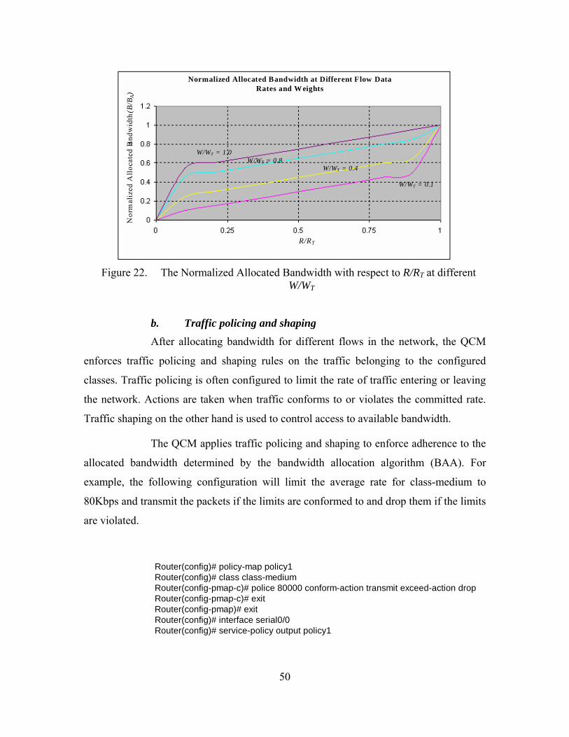
R/RT

Normalized Allocated Bandwidth at Different Flow Data Rates and Weights

W/WT = 1.0 W/WT = 0.8

W/WT = 0.4

W/WT = 0.1

Nor

mal

ized

Allo

cate

d Ba

ndw

idth

(B/B

A)

Figure 22. The Normalized Allocated Bandwidth with respect to R/RT at different

W/WT

b. Traffic policing and shaping After allocating bandwidth for different flows in the network, the QCM

enforces traffic policing and shaping rules on the traffic belonging to the configured

classes. Traffic policing is often configured to limit the rate of traffic entering or leaving

the network. Actions are taken when traffic conforms to or violates the committed rate.

Traffic shaping on the other hand is used to control access to available bandwidth.

The QCM applies traffic policing and shaping to enforce adherence to the

allocated bandwidth determined by the bandwidth allocation algorithm (BAA). For

example, the following configuration will limit the average rate for class-medium to

80Kbps and transmit the packets if the limits are conformed to and drop them if the limits

are violated.

Router(config)# policy-map policy1Router(config)# class class-mediumRouter(config-pmap-c)# police 80000 conform-action transmit exceed-action dropRouter(config-pmap-c)# exitRouter(config-pmap)# exitRouter(config)# interface serial0/0Router(config)# service-policy output policy1

50

The QCM applies traffic shaping on configured classes to allow flexible or

strict bandwidth allocation. For example, the following configuration allocates 300Kbps

to class-high and enables peak shaping, which allows throughput up to 512Kbps if

enough bandwidth is available on the interface.

Router(config)# policy-map policy1Router(config-pmap)# class class-highRouter(config-pmap-c)# bandwidth 300Router(config-pmap-c)# shape peak 512000Router(config-pmap-c)# exitRouter(config-pmap)# exitRouter(config)# interface serial 0/0Router(config-if)# service-policy output policy1

c. The response to network congestions and link failures The edge router starts to drop packets to avoid congestion by randomly

dropping packets from different flows. The QCM needs to make sure that high-priority,

packet loss-sensitive, and delay sensitive flows are not affected by the congestion

avoidance mechanism. This can be achieved by reconfiguring the maximum queue length

allocated for each traffic class. When detecting congestions, the QCM reduces the queue

lengths of lower priority classes. This causes the lower priority traffic to suffer most of

the packets dropouts. Also, traffic policing helps to drop traffic that violates the data rate

limitations.

G. WIRELESS SENSOR NETWORKS REGISTRATION PROTOCOL (WSNRP)

WSNRP is a protocol that will be used to facilitate, prompt, and improve the

communication between applications on the Internet from one side and WSNs from the

other side. The protocol is described and discussed in detail in Appendix A.

In dynamic environments, where new sensor networks appear and others

disappear or die, sensor-applications need to know exactly what sensor networks are

available, what kind of tasks they can carry on, and what type of sensors they have (i.e.,

temperature, humidity, barometric-pressure, etc.). So, a registration server will be able to

give exact information to the requested application about the currently available WSNs

and how to reach them promptly in a very dynamic environment. In a similar way, WSNs

51

52

need to know who the concerned customers (applications) are, how they can be reached,

and what topics (type of information) they are interested in. WSNRP will make accessing

WSNs easier, flexible, and more efficient. WSNRP is introduced in this thesis, as part of

the integration effort between WSNs and the Internet, and to address the following

integration-related issues:

1. Maintain a centralized database of all registered sensor-applications and

WSNs.

2. Help provide QoS functionality based on the registration information.

3. The registration of the reliability topics supported by a WSN helps

applications on the Internet to select the suitable WSNs that satisfy the

applications’ reliability requirements.

4. WSNRP minimizes the number of packets traversed through the

integration link by more than 50% on average.

5. WSNRP helps applications discover the available WSNs and explore their

capabilities.

6. WSNRP makes WSNs more secure by allowing WSNs to only release

information for registered applications.

Appendix A describes the operation of the WSNRP, types of messages, and

message formats.

H. SUMMARY

The proposed integration module aims to help achieve the optimum performance

of the network by utilizing a self-adaptive QoS platform. The integration controller is the

core of the integration module, which registers, monitors, and controls traffic and QoS

parameters. The next chapter discusses the performance analysis of the integration

module.

53

V. PERFORMANCE ANALYSIS

A. INTRODUCTION

This chapter describes the lab setup and procedures to measure the performance

of the proposed integration module. The performance will be measured in terms of traffic

parameters such as throughput, delay, and inter-arrival time. The performance of the

integration module will be measured and compared to the performance of the fair

queuing (FQ) system under the same traffic conditions. The contribution of the WSNRP

will also be presented in this chapter.

B. LABORATORY SETUP

1. Equipment and software components

Figure 23 shows the simulation setup of the integration module at the Naval

Postgraduate School’s Advanced Networking Laboratory. This setup will be used to test

and measure the performance of the integration module.

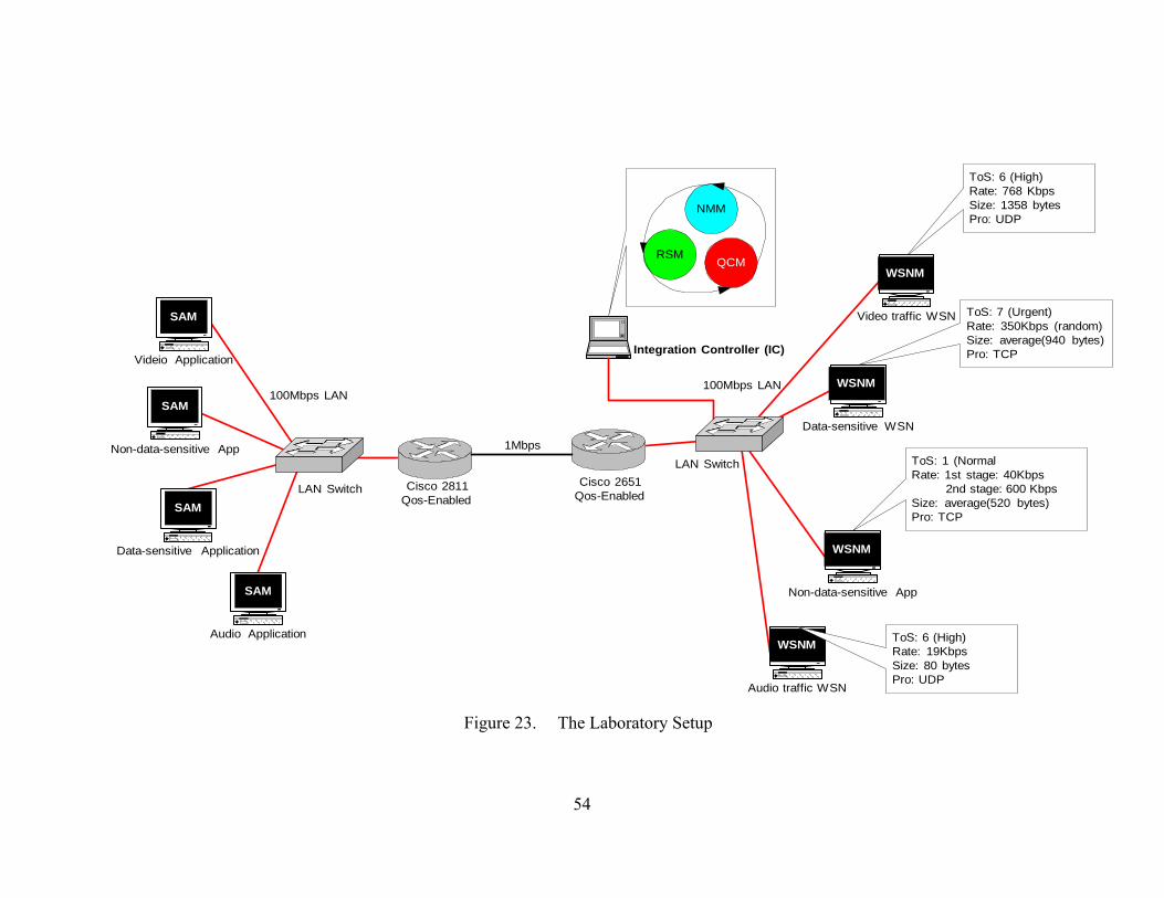
ToS: 6 (High)Rate: 768 KbpsSize: 1358 bytesPro: UDP

Video traffic WSN ToS: 7 (Urgent)Rate: 350Kbps (random)Size: average(940 bytes)Pro: TCP

Data-sensitive WSN

ToS: 1 (NormalRate: 1st stage: 40Kbps 2nd stage: 600 KbpsSize: average(520 bytes)Pro: TCP

Non-data-sensitive App

Audio traffic WSN

Videio Application

Non-data-sensitive App

Data-sensitive Application

Audio Application

Cisco 2651Qos-Enabled

Cisco 2811Qos-Enabled

1Mbps

100Mbps LAN100Mbps LAN

Integration Controller (IC)

NMM

QCMRSM

SAM

SAM

SAM

SAM

WSNM

WSNM ToS: 6 (High)Rate: 19KbpsSize: 80 bytesPro: UDP

WSNM

WSNM

LAN Switch

LAN Switch

Figure 23. The Laboratory Setup

54

55

As shown in Figure 23, the laboratory setup consists of two QoS-enabled routers

(Cisco™ 2651 and 2811) connected by a 1 Mbps serial link, an integration controller

(IC), four personal computers (PCs) connected to a LAN switch to simulate applications

on the Internet, and another four PCs connected to another LAN switch to simulate

WSNs. The IC has three running software components: RSM, NMM, and QCM. Each

computer on the wireless sensor network's side has a software component called the

wireless sensor network module (WSNM). Similarly, each computer on the Internet side

runs a software component called the sensor application module (SAM).

Both the WSNMs and the SAMs are developed to simulate the wireless sensor

networks and the sensor-applications, respectively. The WSNM was built to behave

exactly the same way a wireless sensor network does. Each WSNM module was built

with the following features and capabilities:

1. The ability to respond to queries received from users on the Internet.

2. Generates both periodic and random packets to simulate proactive and

reactive networks, respectively.

3. Generates fixed and variable length packets.

4. Registers with the registration service manager (RSM), and includes

registering priorities, reliabilities and supported topics.

5. Maintains a local registration information file (RIF).

Also, SAMs were built to behave exactly the same way the real applications on

the Internet do. Each SAM represents one sensor-application. SAMs also have the ability

to register with the RSM, keep a local RIF, and send/receive queries and events to and

from wireless sensor networks.

2. Procedures Four different characteristics flows were subjected to two different queuing

systems in two separate experiments. The first experiment subjected the four flows to a

flow-based fair queuing (FQ) system, while the other experiment subjected them to the

control of the integration controller (IC). After five minutes from starting each

experiment, the data rate of one of the flows (non-sensitive data flow) will be suddenly

56

increased to a higher rate. Data rates of other flows will remain the same over the entire

experiment period.

In the first experiment, FQ was implemented on both edge routers. In the second

experiment, FQ was kept running on the Internet side (Cisco™ 2811), while the

integration controller (IC) took control over the edge router on the wireless sensor

network's side (Cisco™ 2651XM). The integration module assumed no control over the

router on the Internet side.

In order to fully evaluate the performance of the integration module, four different

traffic scenarios have been setup on both sides of the module. The four traffic scenarios

aim to represent the most common traffic patterns that traverse the link between the

Internet and the WSNs. All the flows are assumed to be registered. The four traffic

scenarios as shown in Figure 23 are:

• Video stream – This is a registered UDP video streaming flow with an

average packet size of 1,358 bytes and 768 Kbps data rate. The video flow

was registered as a high-priority class flow (TOS = 6).

• Sensitive data flow – This flow represents registered, urgent-priority class

(TOS=7), and exponentially distributed burst series. The time between two

adjacent bursts is exponentially distributed with a mean value of 50

milliseconds. The burst itself is Gaussian with a mean value of 5

milliseconds.

• Non-sensitive data flow – This is a registered TCP and normal-priority

class flow (TOS = 1). The fixed data rate of this flow will be increased

after five minutes from 40 Kbps to 600 Kbps. The purpose of having this

sudden change in data rate is to test the reaction of the integration

controller for injecting a high bit rate flow into the network.

• Audio flow – This is a registered UDP audio streaming flow with

approximately 19 Kbps data rate and 80 bytes packet size. The flow was

registered as a high-priority flow (TOS = 6). Table 5 summaries the

characteristics of the four flows.

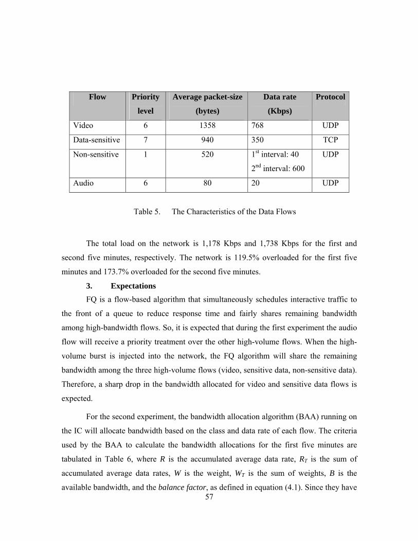
57

Flow Priority

level

Average packet-size

(bytes)

Data rate

(Kbps)

Protocol

Video 6 1358 768 UDP

Data-sensitive 7 940 350 TCP

Non-sensitive 1 520 1st interval: 40

2nd interval: 600

UDP

Audio 6 80 20 UDP

Table 5. The Characteristics of the Data Flows

The total load on the network is 1,178 Kbps and 1,738 Kbps for the first and

second five minutes, respectively. The network is 119.5% overloaded for the first five

minutes and 173.7% overloaded for the second five minutes.

3. Expectations FQ is a flow-based algorithm that simultaneously schedules interactive traffic to

the front of a queue to reduce response time and fairly shares remaining bandwidth

among high-bandwidth flows. So, it is expected that during the first experiment the audio

flow will receive a priority treatment over the other high-volume flows. When the high-

volume burst is injected into the network, the FQ algorithm will share the remaining

bandwidth among the three high-volume flows (video, sensitive data, non-sensitive data).

Therefore, a sharp drop in the bandwidth allocated for video and sensitive data flows is

expected.

For the second experiment, the bandwidth allocation algorithm (BAA) running on

the IC will allocate bandwidth based on the class and data rate of each flow. The criteria

used by the BAA to calculate the bandwidth allocations for the first five minutes are

tabulated in Table 6, where R is the accumulated average data rate, RT is the sum of

accumulated average data rates, W is the weight, WT is the sum of weights, B is the

available bandwidth, and the balance factor, as defined in equation (4.1). Since they have

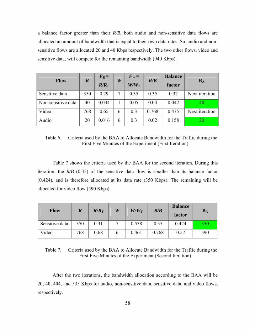
58

a balance factor greater than their R/B, both audio and non-sensitive data flows are

allocated an amount of bandwidth that is equal to their own data rates. So, audio and non-

sensitive flows are allocated 20 and 40 Kbps respectively. The two other flows, video and

sensitive data, will compete for the remaining bandwidth (940 Kbps).

Flow R FR =

R/RTW

FW =

W/WTR/B

Balance

factor BA

Sensitive data 350 0.29 7 0.35 0.35 0.32 Next iteration

Non-sensitive data 40 0.034 1 0.05 0.04 0.042 40

Video 768 0.65 6 0.3 0.768 0.475 Next iteration

Audio 20 0.016 6 0.3 0.02 0.158 20

Table 6. Criteria used by the BAA to Allocate Bandwidth for the Traffic during the First Five Minutes of the Experiment (First Iteration)

Table 7 shows the criteria used by the BAA for the second iteration. During this

iteration, the R/B (0.35) of the sensitive data flow is smaller than its balance factor

(0.424), and is therefore allocated at its data rate (350 Kbps). The remaining will be

allocated for video flow (590 Kbps).

Flow R R/RT W W/WT R/B Balance

factor BA

Sensitive data 350 0.31 7 0.538 0.35 0.424 350

Video 768 0.68 6 0.461 0.768 0.57 590

Table 7. Criteria used by the BAA to Allocate Bandwidth for the Traffic during the First Five Minutes of the Experiment (Second Iteration)

After the two iterations, the bandwidth allocation according to the BAA will be

20, 40, 404, and 535 Kbps for audio, non-sensitive data, sensitive data, and video flows,

respectively.

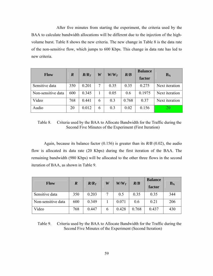
59

After five minutes from starting the experiment, the criteria used by the

BAA to calculate bandwidth allocations will be different due to the injection of the high-

volume burst. Table 8 shows the new criteria. The new change in Table 8 is the data rate

of the non-sensitive flow, which jumps to 600 Kbps. This change in data rate has led to

new criteria.


factor BA

Sensitive data 350 0.201 7 0.35 0.35 0.275 Next iteration

Non-sensitive data 600 0.345 1 0.05 0.6 0.1975 Next iteration

Video 768 0.441 6 0.3 0.768 0.37 Next iteration

Audio 20 0.012 6 0.3 0.02 0.156 20

Table 8. Criteria used by the BAA to Allocate Bandwidth for the Traffic during the Second Five Minutes of the Experiment (First Iteration)

Again, because its balance factor (0.156) is greater than its R/B (0.02), the audio

flow is allocated its data rate (20 Kbps) during the first iteration of the BAA. The

remaining bandwidth (980 Kbps) will be allocated to the other three flows in the second

iteration of BAA, as shown in Table 9.


factor BA

Sensitive data 350 0.203 7 0.5 0.35 0.35 344

Non-sensitive data 600 0.349 1 0.071 0.6 0.21 206

Video 768 0.447 6 0.428 0.768 0.437 430

Table 9. Criteria used by the BAA to Allocate Bandwidth for the Traffic during the Second Five Minutes of the Experiment (Second Iteration)

60

After two iterations, the bandwidth allocation according to the BAA will be 20,

206, 344, and 430 Kbps for audio, non-sensitive data, sensitive data, and video flows,

respectively.

C. DATA COLLECTION AND ANALYSIS TOOLS

Ethereal, an open source packet sniffer program, was used for capturing packets

that traversed the integration link. A number of Perl scripts were developed for this thesis

to obtain statistical parameters from captured packets. Table 10 lists those scripts along

with their functions. Also, Microsoft Excel’s data analysis tools were used to plot some

statistical results.

Script Name Function

TCP-throughput.pl Calculates the throughput along the capture time.

TCP-delay-drop.pl Calculates delay and number of dropped packets.

TCP-RTT.pl Calculates the round-trip-time for acknowledged packet.

UDP-delay-drop.pl Calculates delay and number of dropped packets.

UDP-throughput.pl Calculates the throughput along the capture time.

Table 10. Perl Scripts Used to Extract Statistical Information from Collected Packets

D. RESULTS AND ANALYSIS The following sections describe and analyze the results obtained from the two

experiments.

1. Throughput Figures 24 and 25 show the throughput for the two experiments. Figure 24 shows

the throughput when the four flows were subjected to FQ, while Figure 25 shows the

throughput for the same flows when they were subjected to the control of the IC. It is

crystal clear that under the fair queuing system, both video and sensitive data flows have

suffered a significant decrease in their throughputs when the non-sensitive data flow

flooded the network with a 600 Kbps burst. In less than 10 seconds, the throughput of the

video flow has sharply decreased from an average throughput of 715.14 Kbps during the

first five minutes, to 484.53 Kbps during the second five minutes, a 32% decrease. For

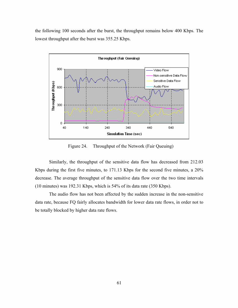
the following 100 seconds after the burst, the throughput remains below 400 Kbps. The

lowest throughput after the burst was 355.25 Kbps.

Figure 24. Throughput of the Network (Fair Queuing)

Similarly, the throughput of the sensitive data flow has decreased from 212.03

Kbps during the first five minutes, to 171.13 Kbps for the second five minutes, a 20%

decrease. The average throughput of the sensitive data flow over the two time intervals

(10 minutes) was 192.31 Kbps, which is 54% of its data rate (350 Kbps).

The audio flow has not been affected by the sudden increase in the non-sensitive

data rate, because FQ fairly allocates bandwidth for lower data rate flows, in order not to

be totally blocked by higher data rate flows.

61

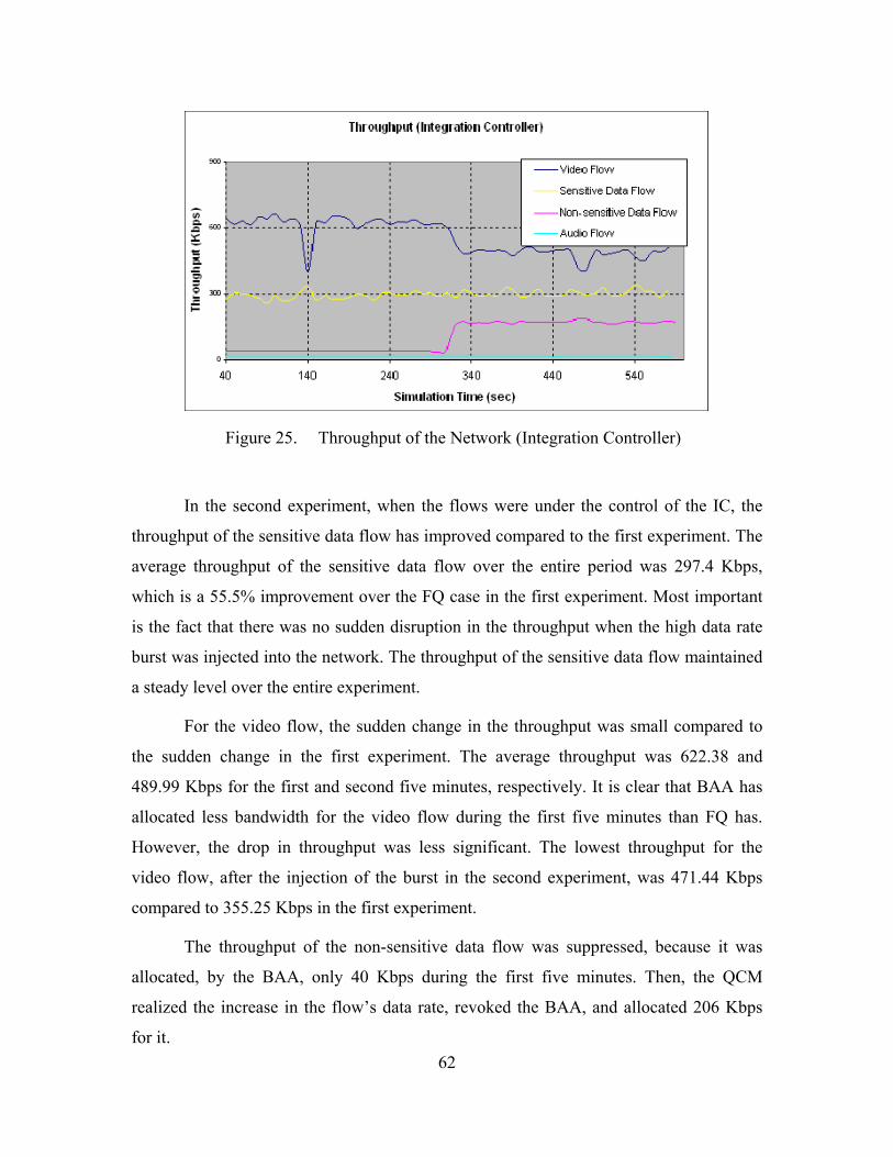
Figure 25. Throughput of the Network (Integration Controller)

In the second experiment, when the flows were under the control of the IC, the

throughput of the sensitive data flow has improved compared to the first experiment. The

average throughput of the sensitive data flow over the entire period was 297.4 Kbps,

which is a 55.5% improvement over the FQ case in the first experiment. Most important

is the fact that there was no sudden disruption in the throughput when the high data rate

burst was injected into the network. The throughput of the sensitive data flow maintained

a steady level over the entire experiment.

For the video flow, the sudden change in the throughput was small compared to

the sudden change in the first experiment. The average throughput was 622.38 and

489.99 Kbps for the first and second five minutes, respectively. It is clear that BAA has

allocated less bandwidth for the video flow during the first five minutes than FQ has.

However, the drop in throughput was less significant. The lowest throughput for the

video flow, after the injection of the burst in the second experiment, was 471.44 Kbps

compared to 355.25 Kbps in the first experiment.

The throughput of the non-sensitive data flow was suppressed, because it was

allocated, by the BAA, only 40 Kbps during the first five minutes. Then, the QCM

realized the increase in the flow’s data rate, revoked the BAA, and allocated 206 Kbps

for it. 62

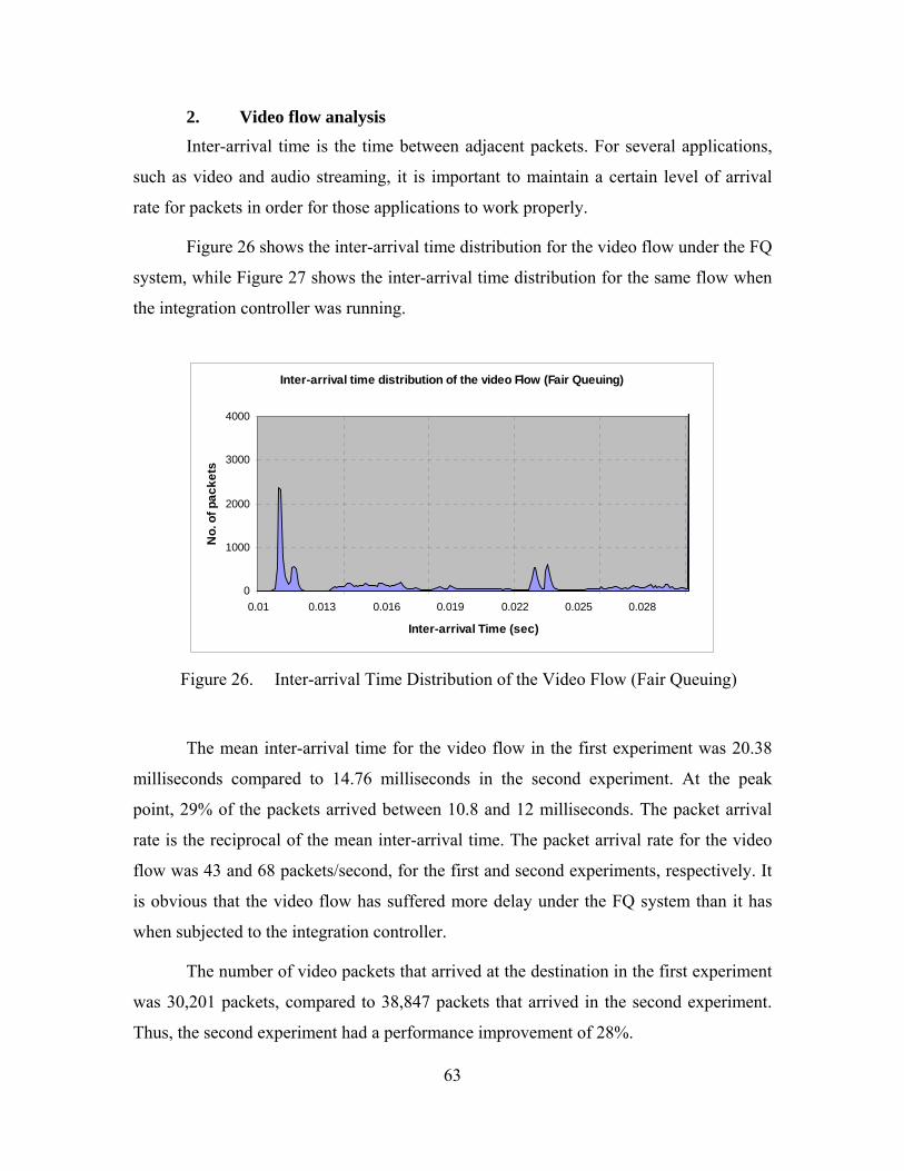
2. Video flow analysis Inter-arrival time is the time between adjacent packets. For several applications,

such as video and audio streaming, it is important to maintain a certain level of arrival

rate for packets in order for those applications to work properly.

Figure 26 shows the inter-arrival time distribution for the video flow under the FQ

system, while Figure 27 shows the inter-arrival time distribution for the same flow when

the integration controller was running.

Inter-arrival time distribution of the video Flow (Fair Queuing)

0

1000

2000

3000

4000

0.01 0.013 0.016 0.019 0.022 0.025 0.028

Inter-arrival Time (sec)

No.

of p

acke

ts

Figure 26. Inter-arrival Time Distribution of the Video Flow (Fair Queuing)

The mean inter-arrival time for the video flow in the first experiment was 20.38

milliseconds compared to 14.76 milliseconds in the second experiment. At the peak

point, 29% of the packets arrived between 10.8 and 12 milliseconds. The packet arrival

rate is the reciprocal of the mean inter-arrival time. The packet arrival rate for the video

flow was 43 and 68 packets/second, for the first and second experiments, respectively. It

is obvious that the video flow has suffered more delay under the FQ system than it has

when subjected to the integration controller.

The number of video packets that arrived at the destination in the first experiment

was 30,201 packets, compared to 38,847 packets that arrived in the second experiment.

Thus, the second experiment had a performance improvement of 28%.

63

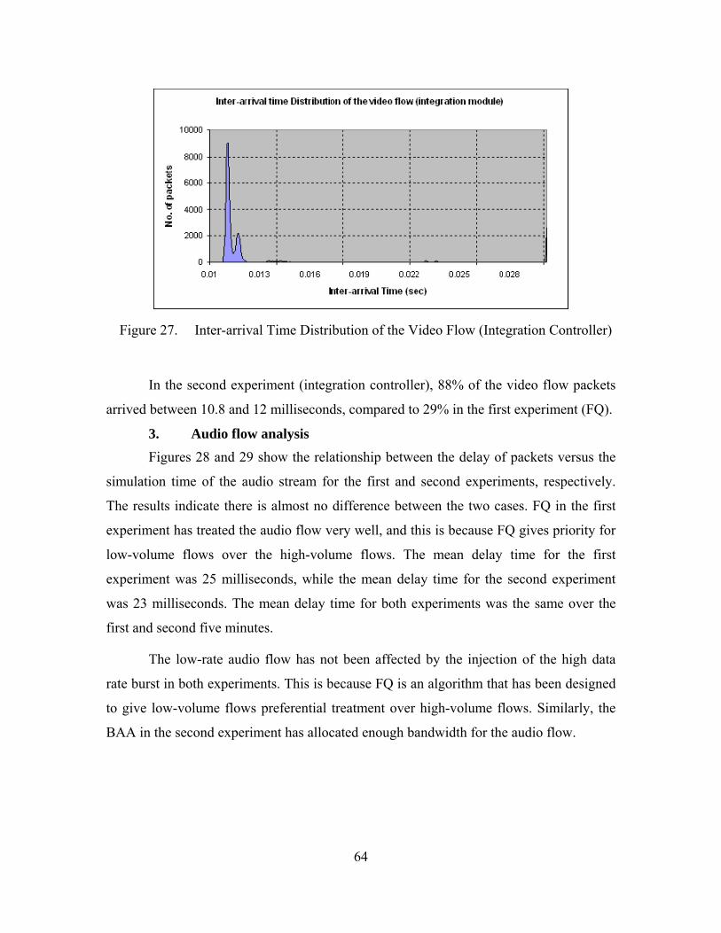
Figure 27. Inter-arrival Time Distribution of the Video Flow (Integration Controller)

In the second experiment (integration controller), 88% of the video flow packets

arrived between 10.8 and 12 milliseconds, compared to 29% in the first experiment (FQ).

3. Audio flow analysis Figures 28 and 29 show the relationship between the delay of packets versus the

simulation time of the audio stream for the first and second experiments, respectively.

The results indicate there is almost no difference between the two cases. FQ in the first

experiment has treated the audio flow very well, and this is because FQ gives priority for

low-volume flows over the high-volume flows. The mean delay time for the first

experiment was 25 milliseconds, while the mean delay time for the second experiment

was 23 milliseconds. The mean delay time for both experiments was the same over the

first and second five minutes.

The low-rate audio flow has not been affected by the injection of the high data

rate burst in both experiments. This is because FQ is an algorithm that has been designed

to give low-volume flows preferential treatment over high-volume flows. Similarly, the

BAA in the second experiment has allocated enough bandwidth for the audio flow.

64

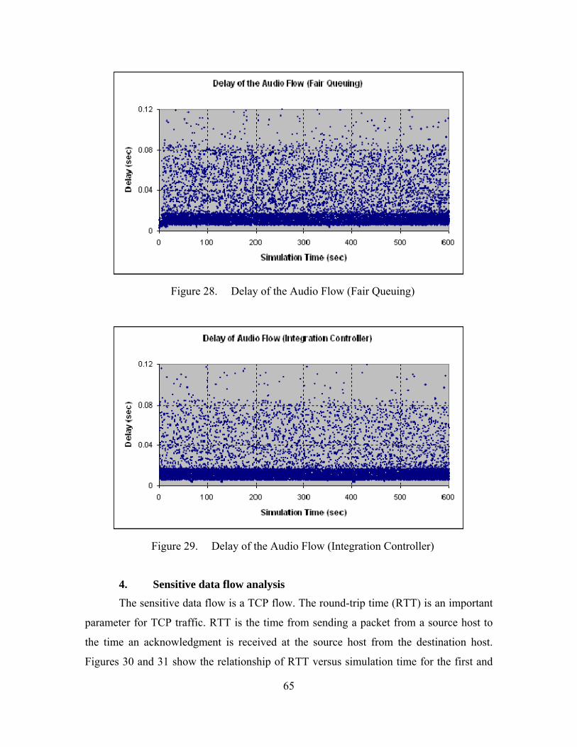
Figure 28. Delay of the Audio Flow (Fair Queuing)

Figure 29. Delay of the Audio Flow (Integration Controller)

4. Sensitive data flow analysis

The sensitive data flow is a TCP flow. The round-trip time (RTT) is an important

parameter for TCP traffic. RTT is the time from sending a packet from a source host to

the time an acknowledgment is received at the source host from the destination host.

Figures 30 and 31 show the relationship of RTT versus simulation time for the first and

65

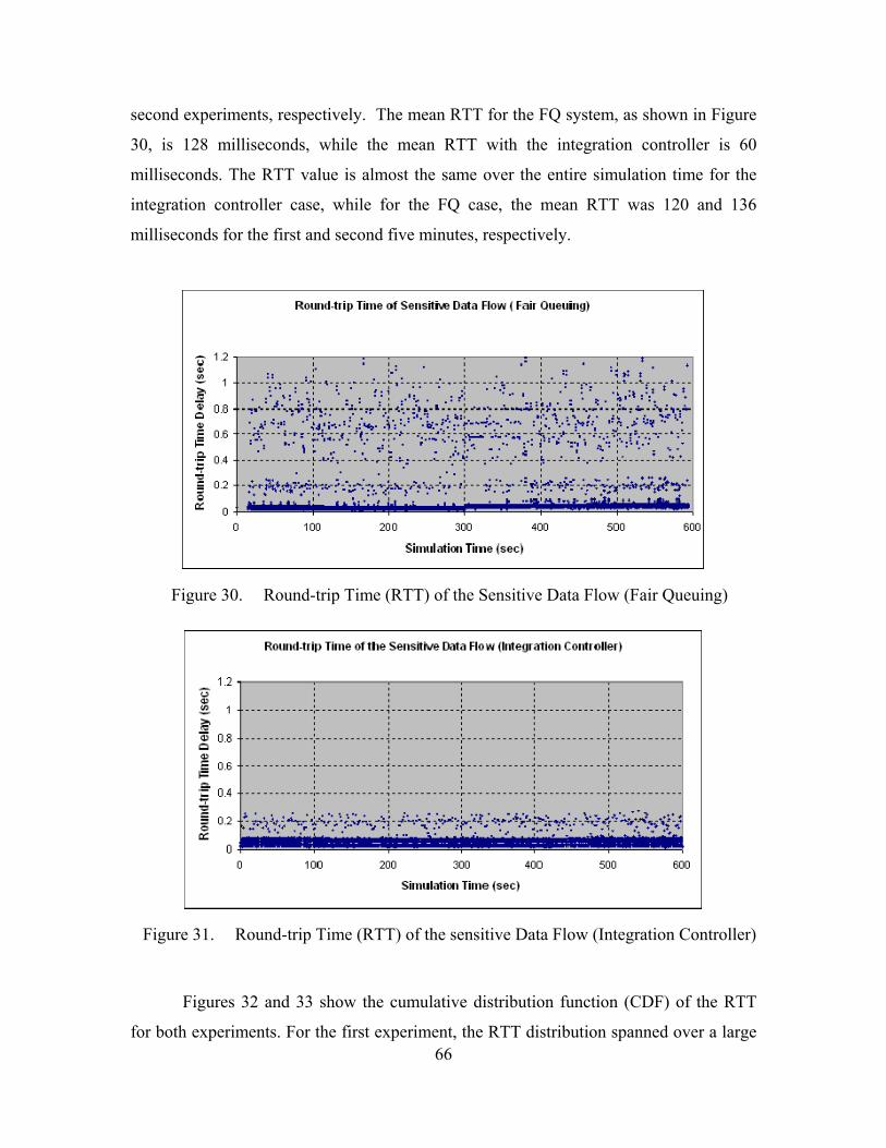
second experiments, respectively. The mean RTT for the FQ system, as shown in Figure

30, is 128 milliseconds, while the mean RTT with the integration controller is 60

milliseconds. The RTT value is almost the same over the entire simulation time for the

integration controller case, while for the FQ case, the mean RTT was 120 and 136

milliseconds for the first and second five minutes, respectively.

Figure 30. Round-trip Time (RTT) of the Sensitive Data Flow (Fair Queuing)

Figure 31. Round-trip Time (RTT) of the sensitive Data Flow (Integration Controller)

66

Figures 32 and 33 show the cumulative distribution function (CDF) of the RTT

for both experiments. For the first experiment, the RTT distribution spanned over a large

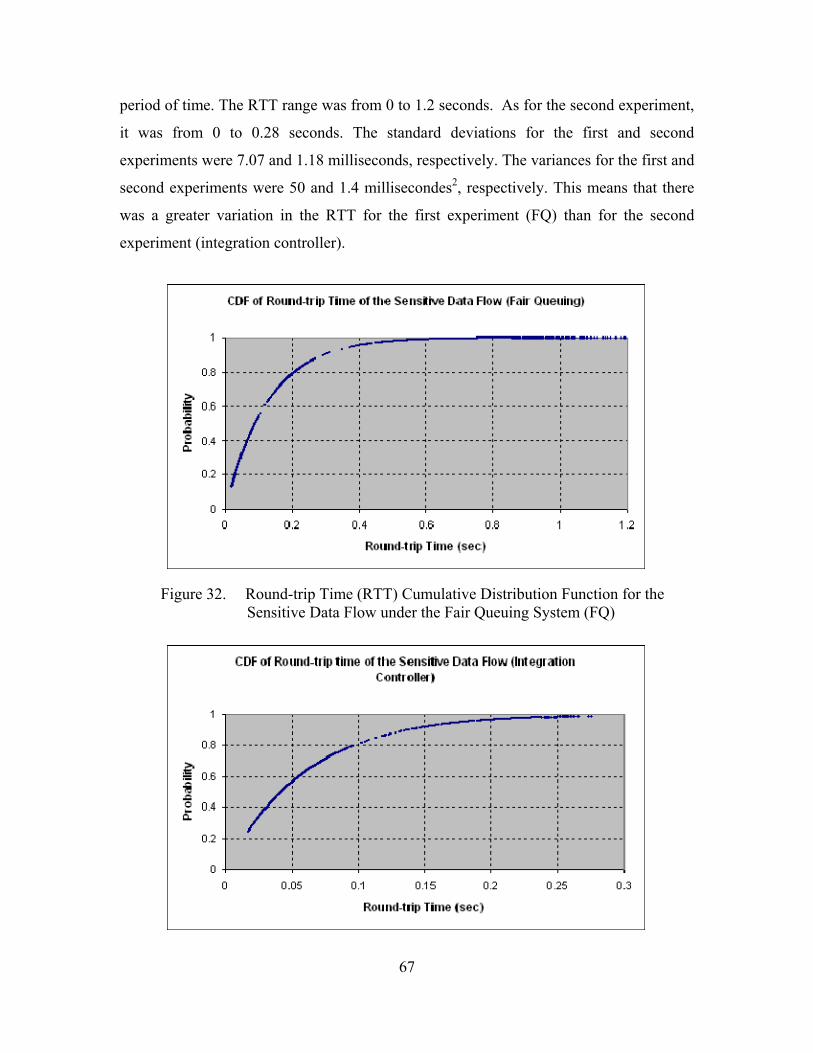
67

period

of time. The RTT range was from 0 to 1.2 seconds. As for the second experiment,

it was from 0 to 0.28 seconds. The standard deviations for the first and second

experiments were 7.07 and 1.18 milliseconds, respectively. The variances for the first and

second experiments were 50 and 1.4 millisecondes2, respectively. This means that there

was a greater variation in the RTT for the first experiment (FQ) than for the second

experiment (integration controller).

Figure 32. Round-trip Time (RTT) Cumulative Distribution Function for the

Sensitive Data Flow under the Fair Queuing System (FQ)

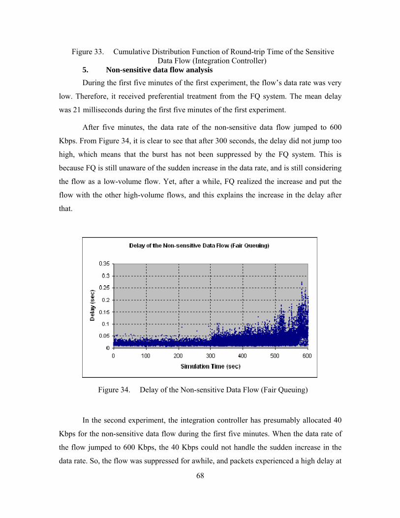
68

e

ean delay

was 21 m

ed to 600

p too

. This is

idering

ut the

that.

Figure 34. Delay of the Non-sensitive Data Flow (Fair Queuing)

In the second experiment, the integration controller has presumably allocated 40

Kbps for the non-sensitive data flow during the first five minutes. When the data rate of

the flow jumped to 600 Kbps, the 40 Kbps could not handle the sudden increase in the

data rate. So, the flow was suppressed for awhile, and packets experienced a high delay at

Figure 33. Cumulative Distribution Function of Round-trip Time of the SensitivData Flow (Integration Controller)

5. Non-sensitive data flow analysis During the first five minutes of the first experiment, the flow’s data rate was very

low. Therefore, it received preferential treatment from the FQ system. The m

illiseconds during the first five minutes of the first experiment.

After five minutes, the data rate of the non-sensitive data flow jump

Kbps. From Figure 34, it is clear to see that after 300 seconds, the delay did not jum

high, which means that the burst has not been suppressed by the FQ system

because FQ is still unaware of the sudden increase in the data rate, and is still cons

the flow as a low-volume flow. Yet, after a while, FQ realized the increase and p

flow with the other high-volume flows, and this explains the increase in the delay after

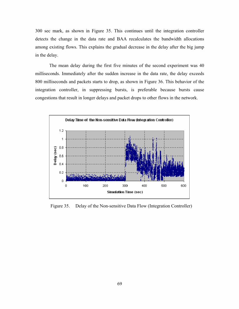
69

300 sec m

detect tions

am

in the de

nt was 40

m

800 m of the

integr

ark, as shown in Figure 35. This continues until the integration controller

s the change in the data rate and BAA recalculates the bandwidth alloca

ong existing flows. This explains the gradual decrease in the delay after the big jump

lay.

The mean delay during the first five minutes of the second experime

illiseconds. Immediately after the sudden increase in the data rate, the delay exceeds

illiseconds and packets starts to drop, as shown in Figure 36. This behavior

ation controller, in suppressing bursts, is preferable because bursts cause

congestions that result in longer delays and packet drops to other flows in the network.

Figure 35. Delay of the Non-sensitive Data Flow (Integration Controller)

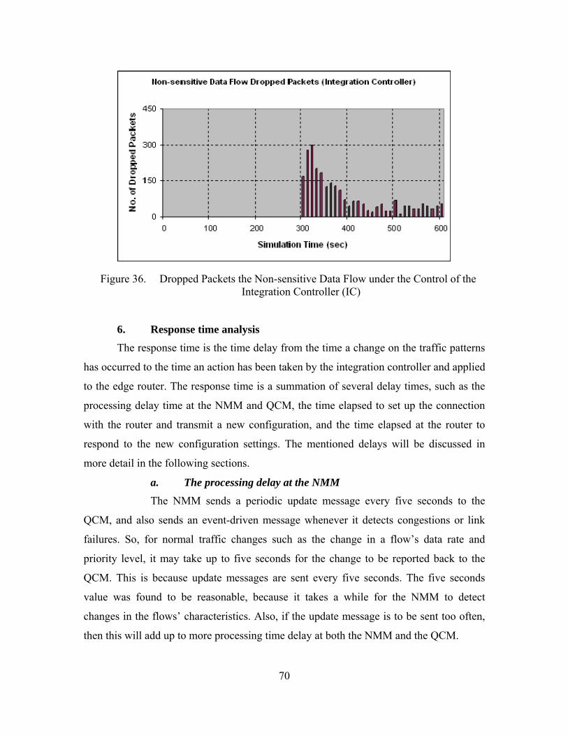
70

Figure 36. Dropped Packets the Non-sensitive Data Flow under the Control of the

has occu plied

with th

mo

QC

failures. So, for normal traffic ch

priority level, it may take up to five seconds for the change to be reported back to the

QCM. s is s are sent every five seconds. The five seconds

value w

Integration Controller (IC)

6. Response time analysis The response time is the time delay from the time a change on the traffic patterns

rred to the time an action has been taken by the integration controller and ap

to the edge router. The response time is a summation of several delay times, such as the

processing delay time at the NMM and QCM, the time elapsed to set up the connection

e router and transmit a new configuration, and the time elapsed at the router to

respond to the new configuration settings. The mentioned delays will be discussed in

re detail in the following sections.

a. The processing delay at the NMM The NMM sends a periodic update message every five seconds to the

M, and also sends an event-driven message whenever it detects congestions or link

anges such as the change in a flow’s data rate and

Thi because update message

as found to be reasonable, because it takes a while for the NMM to detect

changes in the flows’ characteristics. Also, if the update message is to be sent too often,

then this will add up to more processing time delay at both the NMM and the QCM.

71

flows, disappearance of existing flows, changes in

data rates of c nt f congestions and link failures.

For the first th

b. The processing delay at the QCM When receiving a new message from the NMM, the QCM will look for

changes such as, the existence of new

urre lows, and any information regarding

ree cases, the QCM will invoke the BAA to recalculate the bandwidth

allocated for each flow. In order to decide that a certain flow has changed its data rate,

the QCM uses two parameters: accumulated average data rate (R) and instantaneous data

rate (RI), passed by the NMM. If the average instantaneous data rate IR happens to be

greater or less than the accumulated average data rate R for two successive update

intervals, then the QCM assumes an increase or decrease in the data rate. This process

may take at least two periodic intervals, i.e., (2 5)× seconds.

c. Connection set-up time

The QCM is connected to the router through a telnet session. It is possible

that the QCM eps ng the router once in a while.

However, the c

psed at the router before changes at the

configuration f are d through experimentation that changes to

the router’s co

ke the telnet session active by queryi

onnection could be lost for one reason or another, which requires resetting

it. The time from sending the connection setup string to receiving the router’s command

language interface (CLI) was measured and found to be 2 seconds on average. This was

for the case when both the router and the IC were connected to the same 100 Mbps LAN,

i.e., the transmission and propagation delays were negligible. But, if the router is located

in a remote place, then transmission and propagation delays need to be taken into

consideration.

d. Response time of the router

The router’s response time is the most significant delay among the others.

The router’s response time is the time ela

ile reflected. It was observe

nfiguration file by the IC do not take place immediately. This is an issue of

how the router handles traffic scheduling when a user-defined bandwidth allocation

mechanism is implemented. It appears the router does not strictly enforce the bandwidth

allocations decided by the user. Instead, the router tries to use the bandwidth allocations

decided by the user as an argument for its own bandwidth allocation algorithm.

72

ct the new bandwidth allocations decided by the IC when the flow’s data

rate suddenly jumped ws a transient jump in the delay that

begins at the 3

n average

will be added

ptions must be made:

1.

s is L.

sage

Back in Figure 35 which showed the delay for the non-sensitive data flow

under the control of the integration controller, it took the router approximately 100

seconds to refle

to 600 Kbps. The figure sho

00 second mark and lasts until the 400 second mark. During this period,

the QCM has recalculated the bandwidth allocations and sent new configuration

commands to the router. This new bandwidth allocation has not been reflected until the

400 second mark. Afterwards, the delay started to drop gradually until it reaches a steady

point at the 500 second mark.

The response time of the router is much worse if the modifications to the

router’s configurations involve changing the queuing discipline. In this case, the router’s

interface most likely will go down and an additional delay of about 2 minutes o

to the response time. This is why the QCM only utilizes low latency

queuing (LLQ) and avoids switching from one queuing discipline to another. The router’s

response time is a manufacturer issue and can not be addressed in this study

E. THE CONTRIBUTION OF THE WSNRP IN MINIMIZING TRAFFIC One of the main contributions of the wireless sensor networks registration

protocol (WSNRP) is minimizing the traffic exchanged between sensor-applications and

WSNs. Minimizing the exchanged traffic is of significant importance due to the

bandwidth and delay restrictions. In order to prove that applying WSNRP reduces the

exchanged traffic, some assum

The number of sensor-applications in the Internet is N.

2. The number of WSNs is K.

3. The minimum number of request messages that an application can send is

one (assuming there is only one WSN), and the maximum is K (sending

requests to all WSNs).

4. When applying WSNRP, the number of valid (matched) WSN

5. When receiving a request, each WSN will respond back with one mes

to the sender.

As shown in Figure 37, there are two clouds, the Internet cloud with N

applications, and the WSN cloud with K WSNs.

NApplications

KWSN

or the case when WSNRP is not in effect, potentially each application will send

a query

ter 5 Section 1

Figure 37. N-Applications and K-WSNs

F

message to every available WSN, so the maximum number of request messages

sent from applications to WSNs isEquation Chap

M N K= × (5.1)

Each WSN will send back a response message which brings the total number of

exchanged messages to . For example, if there are 4 applications and 5 WSNs,

then N=4 and K=5 and the maximum number of requests is 20, and the maximum

number of exchanged messages is 40 at any given time.

When applying t to matched WSNs,

i.e., to those who have the same topics as the application. So at any given time, this

number

application and

presents the number of unmatched WSNs, so if

sent from

i

( )2 N K×

WSNRP, request messages will only be sen

for an individual application will be a minimum of one (only one WSN matches

the application’s topics) and a maximum of K (all WSNs match the application’s

topics). iL represents the number of matched WSNs for the thi ( )iK L−

re M is the number of request messages

N applications then

i1

N

M L==∑ (5.2)

For the same example above, if L1=2, L2=4, L3=4, and L4=1, then the number of

request messages sent from the 4 applications to the 5 available WSNs is 11. The

73

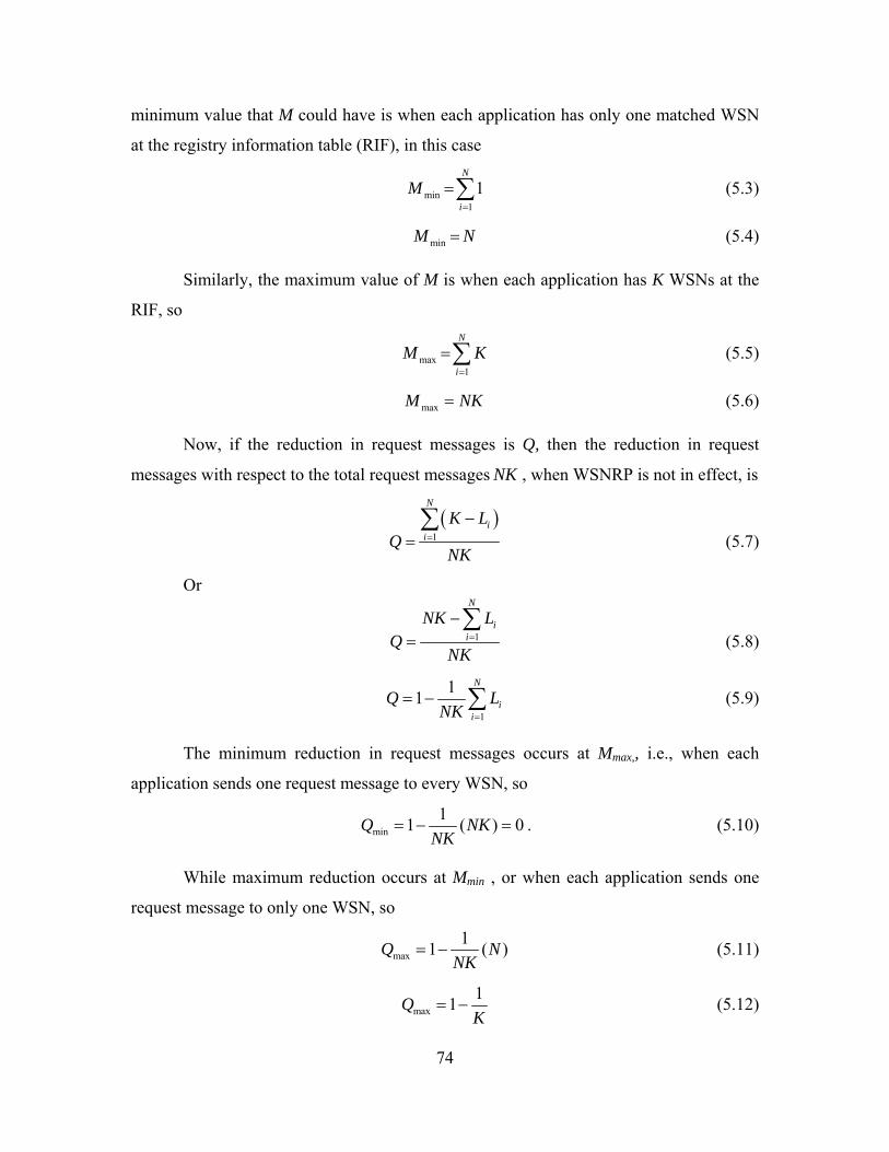
74

minimum value that M could have is when each application has only one matched WSN

at the registry information table (RIF), in this case

min11

N

iM

=

=∑ (5.3)

minM N=

Similarly, the maximum value of M is when each application has K WSNs at the

RIF, so

(5.4)

max1

N

i

M K=

=∑ (5.5)

maxM NK= (5.6)

Now, if the reduction in request messages is Q, then the reduction in request

messages with respect to the total request messages NK , when WSNRP is not in effect, is

( )1

N

i

(5.7) iK L

QNK

=

−=∑

Or

1i

iNK L

Q =

−=

N

NK

∑ (5.8)

1

11N

iLi

QNK =

= − ∑ (5.9)

The minimum reduction in request mess

applica

ages occurs at Mmax,, i.e., when each

tion sends one request message to every WSN, so

min11 (Q NK ) 0

NK= − = . (5.10)

While maximum reduction occurs at Mmin , or when each application

request message to only one WSN, so

sends one

max11 (Q N

NK= − ) (5.11)

max11QK

= − (5.12)

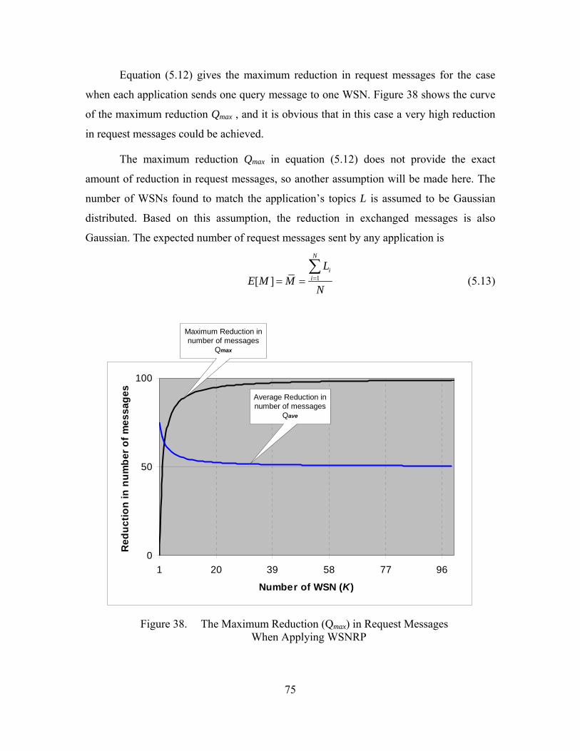
75

Equation (5.12) gives the maximum reduction in request messages for the case

when each application sends one query message to one WSN. Figure 38 shows the curve

of the m

The maximum reduction Qmax in equation (5.

amount of reduction in request messages, so another assumption will be made here. The

numbe

n, the reduction in exchanged messages is also

he expected number of request messages sent by any application is

aximum reduction Qmax , and it is obvious that in this case a very high reduction

in request messages could be achieved.

12) does not provide the exact

r of WSNs found to match the application’s topics L is assumed to be Gaussian

distributed. Based on this assumptio

Gaussian. T

1[ ]

N

ii

LE M M

N== =∑

(5.13)

0

50

num

ber o

f mes

sage

100

1 20 39 58 77 96

Number of WSN (K)

educ

tion

ins

R

Maximum Reduction innumber of messages

Qmax

Average Reduction innumber of messages

Qave

Figure 38. The Maximum Reduction (Qmax) in Request Messages

When Applying WSNRP

76

Recall, minM N= , and maxM NK= , then the average number of request messages

sent by all the applications is

[ ]2

NK NE M M −= = (5.14)

( 12

N KM )−= (5.15)

The average reduction in request messages with respect to the assumption that L

is Gaussian can be expressed as follow

1 ( 1)12ave

N KQNK

−⎛ ⎞= − ⎜ ⎟⎝ ⎠

(5.16)

1 1 , 22 2aveQ K

K= + ≥ (5.17)

So, by applying WSNRP, an average reduction in request messages of more than

50% can be only one

WSN, then there will be no reduction in request messages and applying WSNRP is

meaningless.

F. RY was tested under different conditions. The performance of

e integration module was compared with the perfo

system. The performance of high-volume and high-priority flows showed a significant

provement under the integration module. The p

was almost the same under the two systems.

he following chapter summarizes and concludes the study. Also, unexplored

areas an

achieved. Equation (5.17) is valid for K ≥ 2, because when there is

SUMMAThe integration module

th rmance of the fair queuing (FQ)

im erformance of the low-volume flows

T

d future work will be discussed.

77

VI. CONCLUSIONS AND FUTU

A.

LUSION ule was proposed in this study. The integration module core

compon

on module’s objective was to provide high-

priority

quests from applications on the Internet in order

to access the available WSNs. The registration is carried out by running the wireless

sensor network registration protocol (WSNRP), which has been introduced in this study.

The NMM monitors the traffic in the integration link and sends statistical

information about each flow to the QCM. Also, the NMM informs the QCM about

congestion and link failures.

Based on the registration and monitoring information, the QCM adapts the QoS

configurations at the edge router in such a way that it helps high-priority traffic be

delivered with minimum delay. The QCM uses class-based weighted fair queuing

(CBWFQ) and priority queuing (PQ) to provide differential services. The QCM allocates

class-based bandwidth for each flow using a simple algorithm (i.e., bandwidth allocation

algorithm - BAA).

A simulation network was set up in the Advanced Networking Laboratory at the

Naval Postgraduate School. The goals of the simulation network were to test and measure

the performance of the integration module and compare it with the performance of the

fair queuing system. Four flows with different characteristics were used to simulate the

RE WORK

INTRODUCTION

This chapter summarizes and concludes the research in this study. Related future

research areas are also proposed.

B. CONC

An integration mod

ent was the integration controller (IC), which is a stand-alone laptop with three

software components running on top: the registration service manager (RSM), the QoS

control manager (QCM), and the network monitor manager (NMM). The three software

components work together to register the traffic at the integration link, monitor it, and

then provide an adaptive QoS. The integrati

traffic with preferential service, while maintaining other lower priority traffic.

The RSM receives registration re

78

sensor network c. priority audio

flow, normal-priority non-sensitive data flow, and urgent-priority sensitive data flow.

from the simulation showed an improved performance of

high-vo

55.5%. Also, the results showed that the integration

sudden traffic bursts. When the high data rate burst was

injected

o

systems (integration controller and FQ). This is because the two systems allocate

sufficient bandwidth for low-volum

study because of the shortage of time. The integration module’s response time consisted

of several d

ing a security component

traffi The four flows were: high-priority video flow, high-

The results obtained

lume flows compared with their performance in the FQ system. The performance

of the urgent flow improved by

module was less affected by

into the network, it had a small effect on the high-volume flows’ throughput

compared with the FQ system.

The throughput of the unwanted normal-priority flow (non-sensitive data flow)

was suppressed by 45% under the integration module, which minimized its effect on the

other higher priority flows.

The performance of low-volume flows were almost the same under the tw

e traffic.

The response time of the integration module was only discussed briefly in this

elay times, which included the processing time at both the QCM and the

NMM, the connection setup time with the router, and the router’s response time for

changes to its configuration file.

In conclusion, the objective of this study was met. It is hoped that the results

obtained would help in providing preferential service for the traffic of sensor networks.

C. FUTURE WORK Due to the lack of required resources or time, a number of areas were not

examined and are discussed in the following paragraphs.

1. AddIn addition to the RSM, QCM, and NMM, add a security component, which will

address issues such as protecting WSNs from unauthorized access, guarding against

denial of service attacks, security-based classification of traffic, and other security related

issues.

79

gh

investig

s it different from others.

4. Using real data from sensor nodes

ive more accurate results.

2. More investigation on the response time The response time was briefly investigated during this study. A more thorou

ation is required in order to study the response time under different traffic

scenarios.

3. Modeling the traffic of sensor networks Modeling of the traffic of sensor networks will help in building more efficient

scheduling systems and other QoS functionalities. The traffic of sensor networks has its

own characteristics which make

Along this study, sensor networks were simulated by software modules, which

were built to behave almost like the real sensor networks. Having real sensor network

packets in the network will g

80


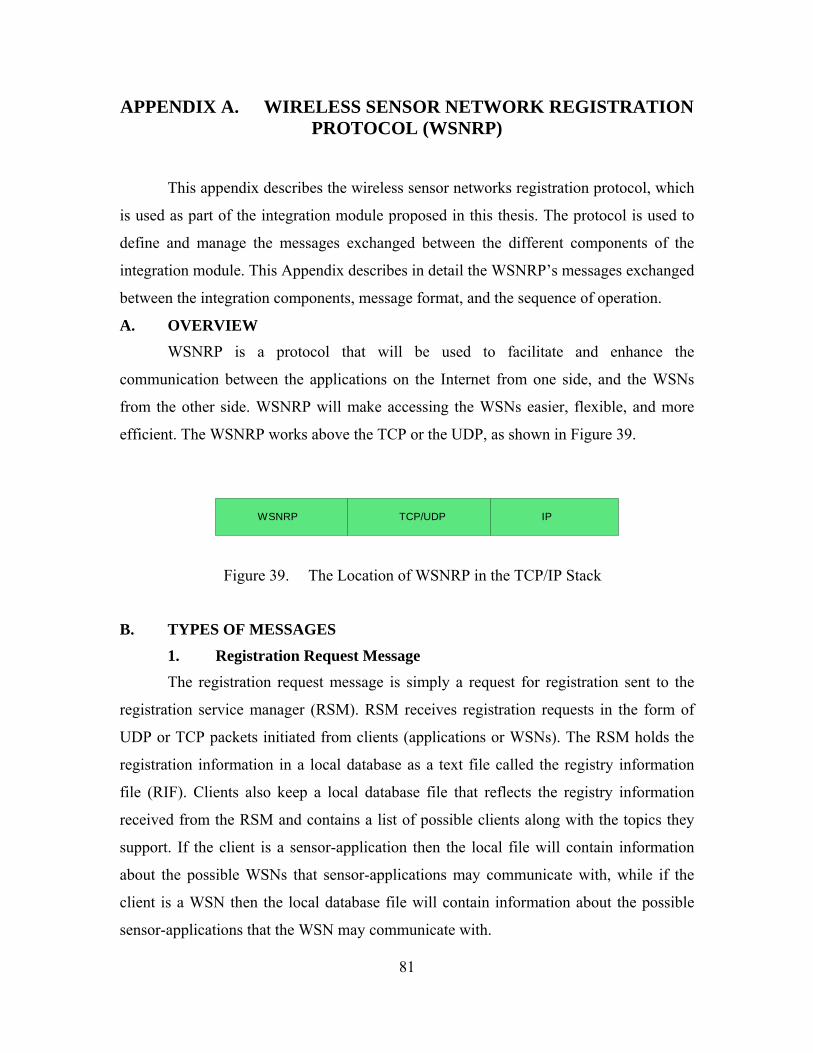
81

APPENDIX A. WIRELESS SENSOR NETWORK REGISTRATION PROTOCOL (WSNRP)

his appendix describes the wireless sensor networks registration protocol, which

is used as part of the integration module proposed in this thesis. The protocol is used to

define and manage the messages exchanged between the different components of the

integration module. This Appendix describes in detail the WSNRP’s messages exchanged

between the integration components, message format, and the sequence of operation.

A. OVERVIEW

SNRP is a protocol that will be used to facilitate and enhance the

communication between the applications on the Internet from one side, and the WSNs

from the other side. WSNRP will make accessing the WSNs easier, flexible, and more

efficient. The WSNRP works above the TCP or the UDP, as shown in Figure 39.

T

W

IPTCP/UDPWSNRP

Figure 39. The Location of WSNRP in the TCP/IP Stack

B. TYPES OF MESSAGES

1. Registration Request Message The registration request message is simply a request for registration sent to the

registration service manager (RSM). RSM receives registration requests in the form of

UDP or TCP packets initiated from clients (applications or WSNs). The RSM holds the

registration information in a local database as a text file called the registry information

file (RIF). Clients also keep a local database file that reflects the registry information

received from the RSM and contains a list of possible clients along with the topics they

support. If the client is a sensor-application then the local file will contain information

about the possible WSNs that sensor-applications may communicate with, while if the

client is a WSN then the local database file will contain information about the possible

sensor-applications that the WSN may communicate with.

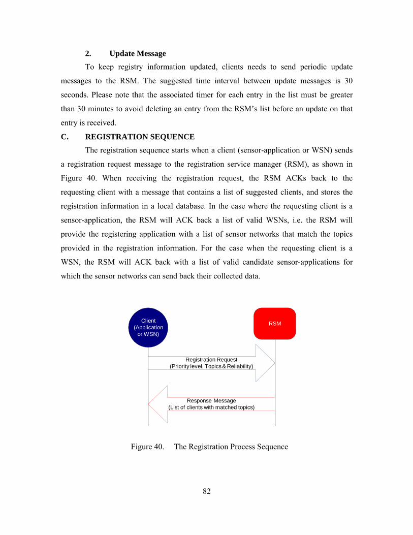
82

To keep registry inf s to send periodic update

messages to the RSM. The suggested time interval between update messages is 30

second

nds

age to the registration service manager (RSM), as shown in

Figure

M will

provide the registering application with a list of sensor networks that match the topics

provided in the registration information. For the case when the requesting client is a

WSN, the RSM will ACK back with a list of valid candidate sensor-applications for

which the sensor networks can send back their collected data.

2. Update Message ormation updated, clients need

s. Please note that the associated timer for each entry in the list must be greater

than 30 minutes to avoid deleting an entry from the RSM’s list before an update on that

entry is received.

C. REGISTRATION SEQUENCE The registration sequence starts when a client (sensor-application or WSN) se

a registration request mess

40. When receiving the registration request, the RSM ACKs back to the

requesting client with a message that contains a list of suggested clients, and stores the

registration information in a local database. In the case where the requesting client is a

sensor-application, the RSM will ACK back a list of valid WSNs, i.e. the RS

RSMClient(Application

or WSN)

Registration Request(Priority level, Topics & Reliability)

Response Message(List of clients with matched topics)

Figure 40. The Registration Process Sequence

83

y, the RSM will start an associated timer that if an

update

iving an update message, the RSM ACKs back with a list of valid

tom rst acknowledging the update message, and

second

contents part length is not

fixed and depends on wither the message is a request or a response message. The content

could be as short as 2 bytes for the case of a request message with only one topic, and as

long as 2,048 bytes for a message that holds up to 256 topics (the maximum). Typically,

response messages are longer than request messages, because they carry additional

information about the clients’ IP addresses and port numbers.

1. Header As mentioned earlier, the WSNPR’s header is 4 bytes long for both request

messages and response messages. Figure 41 shows the header format of the WSNRP for

both request and response messages, whether the client is a sensor-application or WSN.

The WSNRP header consists of the following fields:

For every newly registered entr

has not been received within the timer period, that entry will be deleted from the

database. The timer will be reset when an update is received. The timer value must be

longer than the time intervals between updates; otherwise the timer will be expired before

an update was received.

When rece

cus ers and this serves two goals: fi

, providing the requesting client with an updated list of clients or customers of

interest.

If for any reason the update message did not reach the RSM, then the client needs

to use the current local list for future connections with WSNs and keep sending the

periodic update message until an update message is able to get through to the RSM, and

an update message is received.

D. MESSAGE FORMAT Any WSNPR message consists of two parts: the header and the message contents.

The header part is a fixed 4 bytes long, while the message

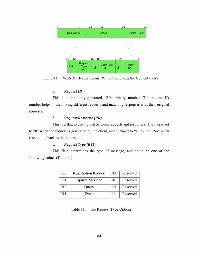
CodesRequest ID

31

Topics Count

84

11

R/R

15

RequestType(RT)

ClientType(CT)

12 19

Priority(P)

23

0 11 237 15

Zero

16 20

Zero

Figure 41.

WSNRP Header Format Without Showing the Content Fields

nse (RR)

Request 100 Reserved

a. Request ID This is a randomly-generated 12-bit binary number. The request ID

number helps in identifying different requests and matching responses with their original

requests.

b. Request/RespoThis is a flag to distinguish between requests and responses. The flag is set

to “0” when the request is generated by the client, and changed to “1” by the RSM when

responding back to the request.

c. Request Type (RT) This field determines the type of message, and could be one of the

following values (Table 11):

000 Registration

001 Update Message 101 Reserved

010 Query 110 Reserved

011 Event 111 Reserved

Table 11. The Request Type Options

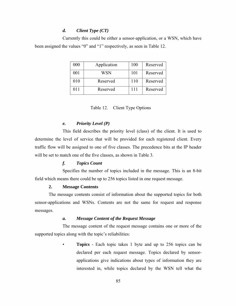
85

d. Client Type (CT) Currently this could be either a sensor-application, or a WSN, which have

been assigned the values “0” and “1” respectively, as seen in Table 12.

000 Application 100 Reserved

001 WSN 101 Reserved

010 Reserved 110 Reserved

011 Reserved 111 Reserved

Table 12. Client Type Options

This field describes the priority level (class) of the client. It is used to

determine the d for each registered client. Every

traffic flow wi

unt ics included in the message. This is an 8-bit

field which me

ents The me ormation about the supported topics for both

sensor-applications and WSNs. Contents ar

messages.

a. The m ore of the

supported topics along with the topic’s reliabilities:

• Topics - Each topic takes 1 byte and up to 256 topics can be

decl a s declared by sensor-

applications give indications about types of information they are

interested in, while topics declared by the WSN tell what the

e. Priority Level (P)

level of service that will be provide

ll be assigned to one of five classes. The precedence bits at the IP header

will be set to match one of the five classes, as shown in Table 3.

f. Topics CoSpecifies the number of top

ans there could be up to 256 topics listed in one request message.

2. Message Contssage contents consist of inf

e not the same for request and response

Message Content of the Request Message essage content of the request message contains one or m

ared per e ch request message. Topic

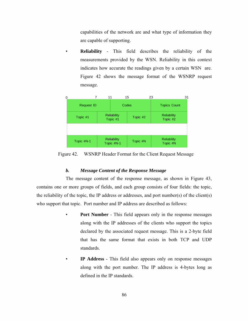
86

ork are and what type of information they

ility of the

measurements provided by the WSN. Reliability in this context

icates the r gs given by a certain WSN are.

ure 42 s he mess or WSNRP request

ssage.

capabilities of the netw

are capable of supporting.

• Reliability - This field describes the reliab

ind how accurate eadin

Fig hows t age f mat of the

me

CodesRequest ID

31

Topics Count

0 11 237 15

Topic #1 ReliabilityTopic #1 Topic #2 Reliability

Topic #2

Topic #N-1 ReliabilityTopic #N-1 Topic #N Reliability

Topic #N

Figure 42. WSNRP Header Format for the Client Request Message

b. Message Content of the Response Message

he topic,

the reli or addresses, and port number(s) of the client(s)

who su

along with the IP addresses of the clients who support the topics

. This is a 2-byte field

The message content of the response message, as shown in Figure 43,

contains one or more groups of fields, and each group consists of four fields: t

ability of the topic, the IP address

pport that topic. Port number and IP address are described as follows:

• Port Number - This field appears only in the response messages

declared by the associated request message

that has the same format that exists in both TCP and UDP

standards.

• IP Address - This field also appears only on response messages

along with the port number. The IP address is 4-bytes long as

defined in the IP standards.

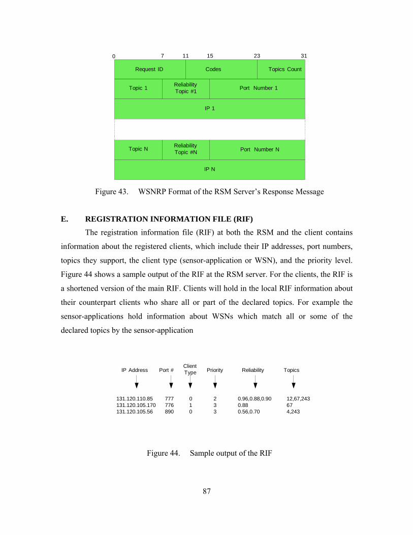
CodesRequest ID

31

87

Topics Count

ZeroTopic 1

0 11 237 15

ReliabilityTopic #1 Port Number 1

ZeroTopic N ReliabilityTopic #N Port Number N

ZeroIP 1

ZeroIP N

Figure 43. WSNRP Format of the RSM Server’s Response Message

E. REGISTRATION INFORMATION FILE (RIF)

The registration information file (RIF) at both the RSM and the client contains

information about the registered clients, which include their IP addresses, port numbers,

topics they ty level.

Figure 44 shows a sample output of the RIF at the RSM server. For the clients, the RIF is

a shortened ve n of mation about

their counterpa

131.120131.12 0 0 3 0.56,0.70 4,243

support, the client type (sensor-application or WSN), and the priori

rsio the main RIF. Clients will hold in the local RIF infor

rt clients who share all or part of the declared topics. For example the

sensor-applications hold information about WSNs which match all or some of the

declared topics by the sensor-application

IP A

131.120.110.85 777 0 2 0.96,0.88,0.90 12,67,243.105.170 776 1 3 0.88 67

0.105.56 89

ddress Port #ClientType Priority TopicsReliability

Figure 44. Sample output of the RIF

88


89

APPENDIX B. QOS INITIAL PROFILE

his appendix contains the initial QoS profile that is used to configure the edge

routers during the initialization phase of the QCM. The following assumptions will be

used:

. The link between the two routers as seen in Figure 23 is a serial link with

1.0 Mbps data rate.

2. Serial 0/0 is the interface that connects the two routers through the T1 link.

3. The clients’ IP addresses will be represented in the format A.B.C.D.

Name QoS-Profile-Initial

T

1

:

General: This profile is basically to configure the edge routers with the initial

configuration. The initial configuration enables classification and creates the needed

classes required to start other profiles.

Description: The following configuration profile is the initial startup configuration of

the QCM. The profile creates 5 traffic classes, creates one policy called set-precedence

to set precedence values according to traffic class, and attaches the policy to an

interface.

Profile

!

class-map class-urgent % creates class Urgent.

match access-group 100 % assign the match criterion.

class-map class-high % creates class High.


class-map class-medium % creates class Medium.


class-map class-low % creates class Low.


class-map class-normal % creates class Normal.


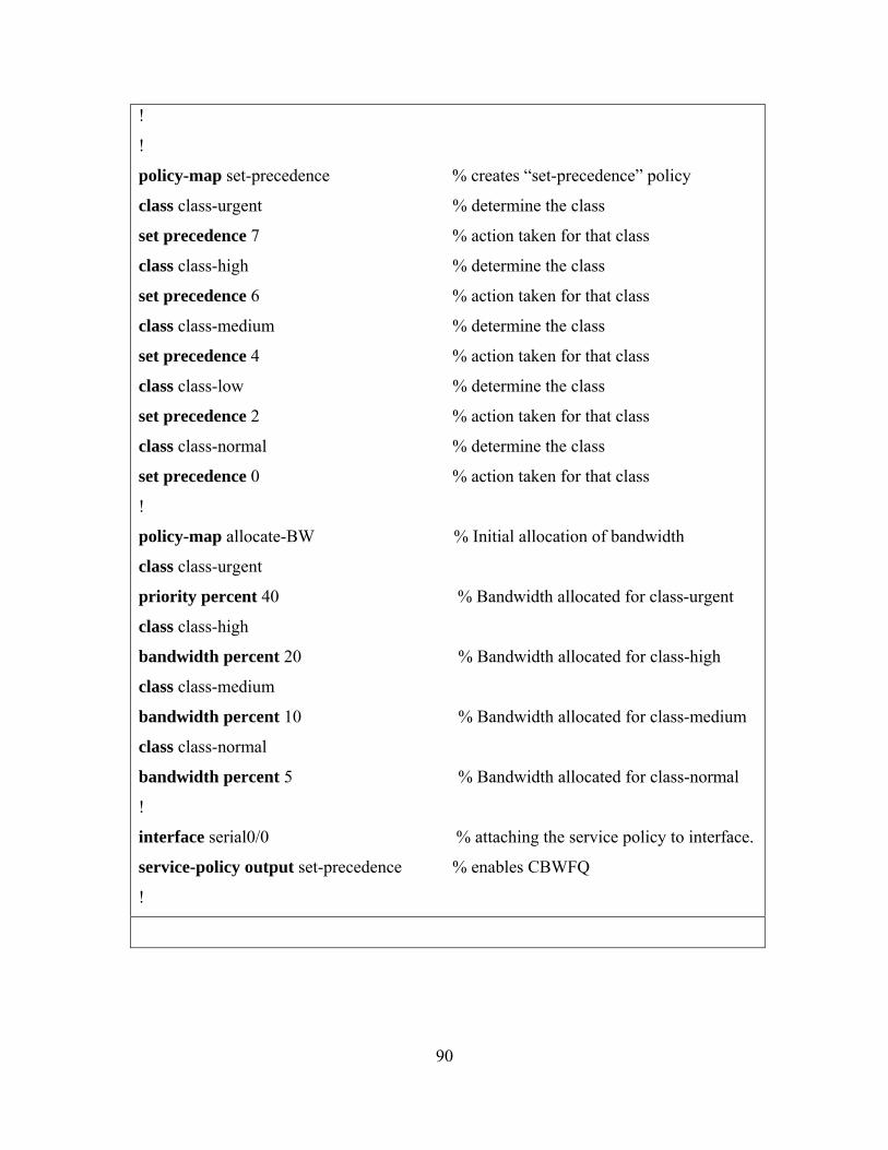
90

!

!

policy

ecedence 7 % action taken for that class

class class-hi

set preceden % action taken for that class

class class-me

set pr den

class class-low % determine the class

% action taken for that class

-high

20 % Bandwidth allocated for class-high

ass class-medium

for class-medium

d for class-normal

olicy to interface.

-map set-precedence % creates “set-precedence” policy

class class-urgent % determine the class

set pr

gh % determine the class

ce 6

dium % determine the class

ece ce 4 % action taken for that class

set precedence 2

class class-normal % determine the class

set precedence 0 % action taken for that class

!

policy-map allocate-BW % Initial allocation of bandwidth

class class-urgent

priority percent 40 % Bandwidth allocated for class-urgent

class class

bandwidth percent

cl

bandwidth percent 10 % Bandwidth allocated

class class-normal

bandwidth percent 5 % Bandwidth allocate

!

interface serial0/0 % attaching the service p

service-policy output set-precedence % enables CBWFQ

!

91

LIST OF REFERENCES

1 Wave 2 The S On line, 003

2 Ma co and Krishn mach e Large-Scale enso Netw ith the I prt, Department of

ngineering, University of Southern Calif.

3 e et Pro col”, ttp://w .html

. Green, Heather, “Tech : ensor Revolution”, Business Week August 25, 2 .

. Z´u˜niga Z., r a a, Bhaskar, “Integrating FuturWireless S r orks w nternet”, Technical ReoElectrical E ornia, Los Angeles, CA 90089, USA

. RFC 791, “Int rn to h ww.faqs.org/rfcs/rfc791 , last accessed

4 Sensor information ications, [see

ireless Communications], pp. 52 –

5. Bejerano, Y., “Efficient Integration of Multihop Wireless and Wired Networks with QoS Constraints”, IEEE/ACM Transactions on Networking, Volume:

6 eiro, A.A.F., MANNA: A management ns

7 ble EE

Conference on Mobile Computing and Networks (MobiCom 2000),

8 nstitute of Computer Science, http://www.sics.se/

on August 2005.

. Chien-Chung, Shen, Srisathapornphat, C. and Jaikaeo, C., “networking architecture and applications”, IEEE Personal Communalso IEEE W Volume: 8, Issue: 4, Aug. 2001,59.

12, Issue: 6, Dec 2004, pp: 1064 – 1078.

. Ruiz, L. B., Nogueira, J. M. and LourArchitecture for Wireless Sensor Networks, IEEE CommunicatioMagazine, Volume: 41, Issue: 2, Feb 2003, pp. 116 – 125.

. Intanagonwiwat, C., Govindan, R. and Estrin, D., “Directed Diffusion: A Scalaand Robust Communication Paradigm for Sensor Networks,” ACM/IEInternational August 2000, Boston, Massachusetts, pp. 56-67.

. The Swidsh I , last accessed on

9 Dunkels, A., Voigt, T. and Alonso, J., “Connecting Wireless Sensor Networks

10. Cisco™ IOS Quality of Service Solutions Configuration Guide, Release 12.2, Cisco™ Systems, 2005, http://www.cisco.com/application/pdf/en/us/guest/products/ps4032/c2001/ccmigr

August 2005.

.

with the Internet”, ERCIM News Online Edition, No. 57, April 2004.

ation_09186a008011dfed.pdf, last accessed on August 2005.

11. Microsoft™ Windows© Server System Website, http://www.microsoft.com/technet/prodtechnol/windowsserver2003/library/Server

92

Help/3d556d54-56eb-4412-a2a9-3c97387ec2b3.mspx, last accessed on August 2005.

ork performance including dependability”

12. ITU-T Recommendation E.800 (08/94) “Terms and definitions related to quality

of service and netw

13. RFC 1946, “Native ATM Support for ST2+”, http://www.cis.ohio-state.edu/htbin/rfc/rfc1946.html, last accessed on August 2005.

Stallings, W., High Speed Networks and Internets, Performance and Quality of 14.

Service, Second Edition, Prentice Hall PTR, Upper Saddle River, NJ, USA.

15. urce Reservation Protocol (RSVP). IETF RFC 2205, September Braden et al. Reso1997, http://www.ietf.org/rfc/rfc2205.txt, last accessed August 2005.

Nagle, John B., “On Packet Switches with Infinite Storage", IEEE Transactions on Communication, Vol. 35, No. 4, Apr1987, pp. 435-438.

16.

17. Floyd, S. and Jacobson, V., “Random Early Detection gateways for Congestion Avoidance". IEEE/ACM Transactions on Networking, Vol. 1 No. 4, August 1993, pp. 397-413.

18. RFC 2474 – “Definition of the Differentiated Services Field (DS Field) in the IPv4 and IPv6 Headers”, http://www.faqs.org/rfcs/rfc2474.html, last accessed on August 2005.

19. Zhao, F. and Guibas, L., “Wireless Sensor Networks, an Information Processing Approach,” Morgan Kaufmann Publishers, San Francisco, CA, 2004 by Elsevier Inc. pp. 63-102.

802.15.4 IEEE Standard for Information techn

20. ology Telecommunications and s -

information exchange between systems Local and metropolitan area networkSpecific requirements http://standards.ieee.org/getieee802/download/802.15.42003.pdf, last accessed on August 2005

stems,” In

Proceedings of the Sixth International Symposium on Communication Theory and

22.

21. Bulusu, N., Estrin, D., Girod L. and Heidemann, J., “Scalable Coordination for wireless sensor networks: Self-Configuring Localization Sy

Applications (ISCTA 2001), Ambleside, Lake District, UK, July 2001

Tubaishat, M. and Madria, S., “Sensor Networks: An Overview,” Potentials, IEEE Volume 22, Issue 2, April-May 2003, pp. 20-23.

23. Lewis, F., “Wireless Sensor Networks,” Smart Environments: Technologies, Protocols, and Applications, edited by D.J. Cook and S.K. Das, John Wiley, New York, 2004.

http://www.sics.se/

http://www.sics.se/

93

24. obotics.eecs.berkeley.edu/~pister/SmartDust/

Smart Dust Project at Berkeley , http://r , last accessed on September 2005.

25. tation Platform for al Conference on

26. Chandrakasan, Ananthal, Min, Rex, Bhardwaj, Manish, Cho, Seong-Hwan and

27. Kahn, J., Katz, R. and Pister, K., “Next century challenges: Mobile networking

28. Rabaey, J., Ammer J., da Silva, J., Patel, D. and Roundy,S, “PicoRadio Supports

Savvides, A. and Srivastava, M. B., “A Distributed CompuWireless Embedded Sensing”, Proceedings of InternationComputer Design 2002, Freiburg, Germany.

Wang, Alice, "Power Aware Wireless Microsensor Systems", ESSCIRC, Florence, Italy, September 2002.

for smart dust,” in Proc. ACM MobiCom’99, Aug. 1999, pp. 271–228.

Ad Hoc Ultra-Low Power Wireless Networking,” IEEE Computer, Vol. 33, No. 7, pp. 42-48, July 2000.

29. PASTA Microsensor 1.0 Developers Manual, http://pasta.east.isi.edu/documentation/devman/c11.html, last accessed on September 2005.

30. The TinyOS operating System, http://www.tinyos.net/, last accessed on

31. base, http://telegraph.cs.berkeley.edu/tinydb

September 2005.

TinyDB Data , last accessed on

32. and Cisco 2651XM Modular Access Routers,

September 2005.

Cisco 2621XM

http://www.cisco.com/en/US/products/hw/routers/ps259/products_white_paper09

186a00801bbf08.shtml#wp58301, last accessed on August 2005.

Installation Procedures for Cisco 2800 Series Routers, 33. Chassis

http://www.cisco.com/en/US/products/ps5854/products_installation_guide_chapte

r09186a00802c5ab3.html, last accessed on August 2005.

34. Net::Telnet Perl module, Jay Rogers, http://cpan.uwinnipeg.ca/htdocs/Net-

Telnet/Net/Telnet.html, last accessed on August 2005.

35. Net::Telnet::Cisco Perl module, Joshua Keroes, http://cpan.uwinnipeg.ca/htdocs/

Net-Telnet-Cisco/Net/Telnet/Cisco.html, last accessed on August 2005.

http://www.microsoft.com/technet/prodtechnol/windowsserver2003/library/ServerHelp/3d556d54-56eb-4412-a2a9-3c97387ec2b3.mspx

http://standards.ieee.org/getieee802/download/802.15.4-2003.pdf

http://standards.ieee.org/getieee802/download/802.15.4-2003.pdf

94


95

INITIAL DISTRIBUTION LIST

1. efense Technical Information Center t. Belvoir, Virginia

2. Dudley Knox Library

Naval Postgraduate School Monterey, California

3. Chairman Code EC Department of Electrical and Computer Engineering Naval Postgraduate School Monterey, California

. Professor Su Weilian Department of Electrical and Computer Engineering Naval Postgraduate School Monterey, California

5. Professor John C. McEachen Department Naval Postgraduate School Monterey, California

DF

4

of Electrical and Computer Engineering

QoS-enabled integration of wireless sensor networks · PDF fileQoS-enabled integration of...

Documents

Transcript of QoS-enabled integration of wireless sensor networks · PDF fileQoS-enabled integration of...