QFI Core Model Solutions - MEMBER | SOA€¦ · QFI Core Spring 2015 Solutions Page 1 QFI Core...

QFI Core Spring 2015 Solutions

QFI Core Model Solutions

Spring 2015

1. Learning Objectives: 1. The candidate will understand the fundamentals of stochastic calculus as they

apply to option pricing.

Learning Outcomes:

(1a) Understand and apply concepts of probability and statistics important in

mathematical finance.

(1b) Understand the importance of the no-arbitrage condition in asset pricing.

(1i) Define and apply the concepts of martingale, market price of risk and measures in

single and multiple state variable contexts.

Sources:

Neftci, Chapter 2

Commentary on Question:

This question tests candidates’ understanding of stock option pricing, condition of

arbitrage-free in stock option pricing formula, and impact of stock dividend on option

pricing. A majority of candidates did very well on this question.

Solution:

(a) Derive the price of the option assuming (1 ) 1 (1 ).d r u

We can set up a replicating portfolio consisting of φ_1 units of the underlying

stock and φ_2 units of risk-free bond. The simultaneous equations are:

𝜑1𝑆𝑢(1 + 𝛿) + 𝜑2(1 + 𝑟) = 𝐶𝑢

𝜑1𝑆𝑑(1 + 𝛿) + 𝜑2(1 + 𝑟) = 𝐶𝑑

Solving the two equations, we get

𝜑1 =𝐶𝑢−𝐶𝑑

𝑆(1+𝛿)(𝑢−𝑑) and 𝜑2 =

𝑢𝐶𝑑−𝑑𝐶𝑢

(1+𝑟)(𝑢−𝑑)

The value of the option at time 0 is


1. Continued

𝐶 = 𝜑1𝑆 + 𝜑2

=𝐶𝑢 − 𝐶𝑑

𝑆(1 + 𝛿)(𝑢 − 𝑑)𝑆 +

𝑢𝐶𝑑 − 𝑑𝐶𝑢

(1 + 𝑟)(𝑢 − 𝑑)

= 1

1 + 𝑟[(1 + 𝑟)/(1 + 𝛿) − 𝑑

𝑢 − 𝑑𝐶𝑢 +

𝑢 − (1 + 𝑟)/(1 + 𝛿)

𝑢 − 𝑑𝐶𝑑]

let 𝑞 =(1+𝑟)/(1+𝛿)−𝑑

𝑢−𝑑 , we can write C as the expected discounted value of the

option

𝐶 = 1

1 + 𝑟[𝑞𝐶𝑢 + (1 − 𝑞)𝐶𝑑]

(b) Explain why it must be assumed that (1 ) 1 (1 ).d r u

The condition is required for arbitrage-free.

Otherwise, there are arbitrage opportunities by taking either long or short

positions on the stock that could generate guaranteed profits.

Also, if the inequalities did not hold, the quantity q would lie outside of range of

(0, 1) and hence could not represent a probability.

(c) Analyze the impact on the price of the option if the stock dividend is increased to * .

When the dividend 𝛿 is increased, 𝑞 =(1+𝑟)/(1+𝛿)−𝑑

𝑢−𝑑 is decreased if other

parameters remain the same.

The impact on the option price 𝐶 = 1

1+𝑟[𝑞𝐶𝑢 + (1 − 𝑞)𝐶𝑑] depends upon the

payoffs 𝐶𝑢 and 𝐶𝑑:

The value 𝐶 of the option will be lower if 𝐶𝑢 > 𝐶𝑑.

The value 𝐶 of the option will be higher if 𝐶𝑢 < 𝐶𝑑.

No impact if the payoffs are the same on both paths.




Learning Outcomes:


(1c) Understand Ito integral and stochastic differential equations.

(1d) Understand and apply Ito’s Lemma.

(1f) Demonstrate understanding of option pricing techniques and theory for equity and

interest rate derivatives.

(1k) Understand the Black Scholes Merton PDE (partial differential equation).

(1l) Identify limitations of the Black-Scholes pricing formula.

Sources:

Neftci Ch. 10.4, 10.7.1, 12.2, 13.2

Wilmott – Introduces Quantitative Finance Ch. 16.3


Commentary listed underneath question component.

Solution:

(a) Derive , ,t td S v t , the change in the portfolio value, in terms of , ,dt dS and

tdv .


While a number of candidates did not attempt the questions, those candidates who

attempted this question did fairly well. The key is to apply Ito’s Lemma to get the

change of f(St, vt, t) the value at time t of a European derivative with expiration T

and terminal payoff 𝑔(𝑆𝑇) and 𝑈(𝑆𝑡, 𝑣𝑡, 𝑡) the value at time t of a European

derivative with expiration T and terminal payoff ℎ(𝑣𝑇). Some candidates missed a

few terms in the calculations and scored partial credits.


2. Continued

For ease of notations, we suppress the arguments for f(𝑆𝑡, 𝑣𝑡 , t) and denote it as

𝑓 = f(𝑆𝑡, 𝑣𝑡 , t).

By Ito’s Lemma,

df =∂f

∂tdt +

∂f

∂SdS +

∂f

∂𝑣d𝑣 +

1

2𝑣S2 ∂2f

∂S2dt +

1

2𝑣σ2 ∂2f

∂𝑣2dt + 𝑣σSρ

∂2f

∂S ∂𝑣dt

(a-1)

Similar result for dU, namely:

dU=∂U

∂tdt +

∂U

∂SdS +

∂U

∂𝑣d𝑣 +

1

2𝑣S2 ∂2U

∂S2 dt +1

2𝑣σ2 ∂2U

∂𝑣2 dt + 𝑣σSρ∂2U

∂S ∂𝑣dt

(a-2)

Thus, (a-1) and (a-2) lead to the result

𝑑Π = df + δ𝑑S + 𝛾𝑑𝑈 = (∂f

∂t+

1

2𝑣S2 ∂2f

∂S2 dt +1

2𝑣σ2 ∂2f

∂𝑣2 dt + 𝑣σSρ∂2f

∂S ∂𝑣) dt +

γ (∂U

∂t+

1

2𝑣S2 ∂2U

∂S2 +1

2𝑣σ2 ∂2U

∂𝑣2 + 𝑣σSρ∂2U

∂S ∂𝑣) dt + (

∂f

∂S+ γ

∂U

∂S+ δ) dS + (

∂f

∂𝑣+

γ∂U

∂𝑣)d𝑣

(a-3)

(b) Solve for the weights and so as to make the portfolio riskless. Express

the resulting , ,t td S v t with the parameters and obtained.


Candidates did not do well in this question. The key is that the diffusion terms

have to vanish in order to have no randomness (thus riskless). A number of

candidates recognized this however not a lot of them were able to perform the

calculation.

∂f

∂S+ γ

∂U

∂S+ δ = 0

∂f

∂𝜐+ γ

∂U

∂𝜐= 0

(b-1)

Using simple algebra, we have the following results

γ = −

∂f

∂𝜐∂U

∂𝜐

⁄


2. Continued

δ = −∂f

∂S+ (

∂f

∂𝜐∂U

∂𝜐

⁄ )∂U

∂S

(b-2)

𝑑Π = (∂f

∂t+

1

2υS2 ∂2f

∂S2 dt +1

2𝜐σ2 ∂2f

∂𝜐2 dt + 𝜐σSρ∂2f

∂S ∂𝜐) dt −

∂f

∂𝜐∂U

∂𝜐

⁄ (∂U

∂t+

1

2𝜐S2 ∂2U

∂S2 +

1

2𝜐σ2 ∂2U

∂𝜐2 + υσSρ∂2U

∂S ∂𝜐) dt

(b-3)




Learning Outcomes:







(1j) Understand and apply Girsanov’s theorem in changing measures.

Sources:

Wilmott, Paul, Frequently Asked Questions in Quantitative Finance, 2nd Edition Ch. 2:

Q26

An Introduction to the Mathematics of Financial Derivatives, Neftci, Salih, 3rd Edition.

Ch. 2, 6, 8, 11, 12, 14, 15


Candidates did generally well on Part A.

Many candidates attempted a more complex answer to Part B (or skipped it), although

the solution was straightforward.

For Part C, there were several components necessary to prove that W2(t) is a Brownian

motion under the probability measure ℙ2. Candidates received full credit for identifying

three properties, including the independence of increments, the mean and variance.

Part D called for the application of Ito’s lemma and Girsanov’s theorem to a vector

setting. Many candidates received partial credit for identifying this most but had trouble

with its proper formulation.

Part E required the construction of a hedging strategy that showed zero volatility.

Candidates received credit for identifying the components of the hedging strategy (three

assets: S1, S2, and savings account) and the correct derivation of the weights in each

asset class.


3. Continued

Solution:

(a) Derive an expression for k in terms of 2 and

2.

d[ln(e-kt U2 (t)] = -kdt + d(lnU2 (t))

= -kdt + (µ2 dt + σ2 dW(t) -σ22/2 dt)

= (µ2-σ22/2 -k)dt + σ2dW(t)

You need the drift term to equal zero for ln(e-kt U2 (t)) to be a martingale

k = µ2-σ22 /2

(b) Write an expression for the relationship among 1 1, , and 2 2, , and r

necessary for the no-arbitrage condition to hold.


The answer was very straightforward, although some candidates developed the

solution mathematically. No points were awarded or subtracted for this. Some

candidates showed an alternative form of the same expression and were awarded

full credit.

Note that μ2−r

σ2 is the market price of risk

Under a no-arbitrage condition, then: µ1 − r

σ1=

µ2 − r

σ2

(c) Prove that 2W t is a Brownian motion under the probability measure ℙ2.


There were several components necessary to prove that W2(t) is a Brownian

motion under the probability measure ℙ2. Candidates received full credit for

identifying three properties, including the independence of increments, the mean

and variance.

W2(t) − W2(s) = ρ(W1(t) − W1(s)) + √(1 − ρ2) (W0(t) − W0 (s))

1. Since |ρ| ≤ 1, W2 is a linear combination of two continuous Brownian motions,

thus W2 is also continuous

2. Since W2 is a linear combination of two normal distributions, W2 is also

normally distributed. Similarly, W2 has independent increments

3. E[W2(t) − W2(s)] = 0 (straightforward)


3. Continued

4. V[W2(t) − W2(s)] = V[ ρ(W1(t) − W1(s)) + √(1 − ρ2) (W0(t) −

W0 (s))] = ρ2V[W1(t) − W1(s)] + (1 − ρ2)V[W0(t) − W0(s)] =

ρ2(t − s) + (1 − ρ2)(t − s) = t − s

For asset 1, applying Ito’s lemma to 𝑒−𝑟𝑡𝑆1(𝑡), we have that

𝑑(𝑒−𝑟𝑡𝑆1(𝑡)) = 𝑆1(𝑡)𝑑(𝑒−𝑟𝑡) + 𝑒−𝑟𝑡𝑑𝑆1(𝑡)

And given the definition of 𝑑𝑆1(𝑡), under ℙ2

𝑑(𝑒−𝑟𝑡𝑆1(𝑡)) = 𝑒−𝑟𝑡(𝑚1 − 𝑟)𝑆1(𝑡)𝑑𝑡 + 𝑒−𝑟𝑡𝑣1𝑆1(𝑡)𝑑𝑊1(𝑡)

Under ℙ2, this is not a martingale since (𝑚1 − 𝑟) could be ≠ 0

Girsanov’s theorem states if 𝑊1 is a standard Wiener process under ℙ2, there

exists another standard Wiener process, �̃�1, where Q is a martingale measure,

defined as

𝑑�̃�1(𝑡) = 𝑑𝑊1(𝑡) + 𝑑𝑋1(𝑡)

Moving from ℙ2 to Q,

𝑑(𝑒−𝑟𝑡𝑆1(𝑡)) = 𝑒−𝑟𝑡(𝑚1 − 𝑟)𝑆1(𝑡)𝑑𝑡 + 𝑒−𝑟𝑡𝑣1𝑆1(𝑡) (𝑑�̃�1(𝑡) − 𝑑𝑋1(𝑡))

To be a martingale the drift term should be equal to zero, thus

𝑒−𝑟𝑡(𝑚1 − 𝑟)𝑆1(𝑡) − 𝑒−𝑟𝑡𝑣1𝑆1(𝑡)𝑑𝑋1(𝑡) = 0 Thus

𝑑𝑋1(𝑡) =(𝑚1 − 𝑟)

𝑣1𝑑𝑡

For asset 2, also applying Ito’s lemma

𝑑(𝑒−𝑟𝑡𝑆2(𝑡)) = 𝑆2(𝑡)𝑑(𝑒−𝑟𝑡) + 𝑒−𝑟𝑡𝑑𝑆2(𝑡)

And given the definition of 𝑑𝑆2(𝑡), under ℙ2

𝑑(𝑒−𝑟𝑡𝑆2(𝑡)) = 𝑒−𝑟𝑡(𝑚2 − 𝑟)𝑆2(𝑡)𝑑𝑡 + 𝑒−𝑟𝑡𝑣2𝑆2(𝑡)𝑑𝑊2(𝑡)

Since 𝑊2(𝑡) = 𝜌𝑊1(𝑡) + √1 − 𝜌2 𝑊0(𝑡),


3. Continued

𝑑𝑊2(𝑡) = 𝜌𝑑𝑊1(𝑡) + √1 − 𝜌2 𝑑𝑊0(𝑡)

We have

𝑑(𝑒−𝑟𝑡𝑆2(𝑡)) = 𝑒−𝑟𝑡(𝑚2 − 𝑟)𝑆2(𝑡)𝑑𝑡

+ 𝑒−𝑟𝑡𝑣2𝑆2(𝑡) [𝜌𝑑𝑊1(𝑡) + √1 − 𝜌2 𝑑𝑊0(𝑡)]

Girsanov’s theorem states if 𝑊0 is a standard Wiener process under ℙ2, there

exists another standard Wiener process, �̃�0, where Q is a martingale measure,

defined as

𝑑�̃�0(𝑡) = 𝑑𝑊0(𝑡) + 𝑑𝑋0(𝑡)

Moving from ℙ2 to Q, and knowing the definition of 𝑑𝑋1(𝑡) under Q, we have

𝑑(𝑒−𝑟𝑡𝑆2(𝑡)) = 𝑒−𝑟𝑡(𝑚2 − 𝑟)𝑆2(𝑡)𝑑𝑡

+ 𝑒−𝑟𝑡𝑣2𝑆2(𝑡) [𝜌 (𝑑�̃�1(𝑡) − 𝑑𝑋1(𝑡))

+ √1 − 𝜌2 (𝑑�̃�0(𝑡) − 𝑑𝑋0(𝑡))]

To be a martingale the drift term should be equal to zero, thus

𝑒−𝑟𝑡(𝑚2 − 𝑟)𝑆2(𝑡)𝑑𝑡 = 𝑒−𝑟𝑡𝑣2𝑆2(𝑡) [𝜌(𝑑𝑋1(𝑡)) + √1 − 𝜌2 (𝑑𝑋0(𝑡))]

Solving for 𝑑𝑋0(𝑡) we get

𝑑𝑋0(𝑡) =

(𝑚2 − 𝑟)𝑣2

𝑑𝑡 − 𝜌𝑑𝑋1(𝑡)

√1 − 𝜌2

Which can only exist when 1 . Q is the only measure under which 𝑒−𝑟𝑡𝑆1(𝑡)

and 𝑒−𝑟𝑡𝑆2(𝑡) are martingales, otherwise there would be multiple arbitrage free

prices.

(e) Construct a self-financing trading strategy with non-zero weights using the two

assets in Portfolio 2 and the risk-free savings account such that the resulting

portfolio has zero volatility.


3. Continued

Commentary on Question: None

Candidates received full credit for part E if they stated the hedging strategy

components:

Setting up a portfolio using the two assets in portfolio II and the risk free

savings account without volatility and showing the differential equation of the

portfolio under W1(t) terms

Identifying that the volatility coefficient needs to be zero in order to have a

risk-free portfolio

Stating (and showing) the strategy: Long X units of S1, short v1S1X/v2S2 and

lend/borrow the remaining funds in the risk free savings account.

Identifying that since the market price of risk is the same for S1 and S2, the

resulting portfolio has zero volatility




2. The candidate will understand how to apply the fundamental theory underlying

the standard models for pricing financial derivatives. The candidate will

understand the implications for option pricing when markets do not satisfy the

common assumptions used in option pricing theory such as market completeness,

bounded variation, perfect liquidity, etc. The Candidate will understand how to

evaluate situations associated with derivatives and hedging activities.

Learning Outcomes:

(1h) Demonstrate understanding of the differences and implications of real-world

versus risk-neutral probability measures.

(1l) Identify limitations of the Black-Scholes pricing formula.

(2a) Identify limitations of the Black-Scholes pricing formula

(2d) Understand the different approaches to hedging.

(2e) Understand how to delta hedge and the interplay between hedging assumptions

and hedging outcomes.

Sources:

Paul Wilmott, Intro to Quant Finance, 2nd ed., Ch. 6, Ch. 8


The purpose of this question is to test candidates on the pricing a non-standard option

under Black Scholes framework. We further test candidates on deriving the Greeks

associated with the non-standard option and interpreting the meaning on the Greeks.

Solution:

(a) Sketch the payoff diagram of this option at maturity.


This question is designed to help candidate picture the problem solving at hand

and structure the rest of the solution to the problem.

Majority of the candidates were able to get the correct answer.

It is key for the candidate to recognize the payoff diagram has a jump at 𝑆 = 𝐾.


4. Continued

Payoff

,

Payoff = 0,

St St K

St K

K S

(b) Show that TV can be restated as CT

+K I ST

³ K( ) where ( )I A denotes the

indicator function for an event A.


This question is designed to help candidate further understand the problem. That

is, the option at hand can be simplify into two basic options.

One can easily visualize from the diagram in (a) that the only difference between

this option payoff and that of a call option with exercise price K is the value of the

exercise price.

Using indicator functions, one can also show that

VT = STI(ST ≥ K) − KI(ST ≥ K) + KI(ST ≥ K)

= (ST − K)I(ST ≥ K) + KI(ST ≥ K)

= CT + KI(ST ≥ K)

(c) Derive a formula for the value of this option at time 0.

2Hint: Pr TS K N d

Payoff at Maturity


4. Continued


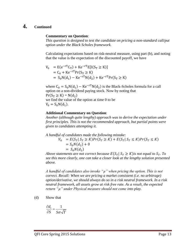
This question is designed to test the candidate on pricing a non-standard call/put

option under the Black Scholes framework.

Calculating expectations based on risk-neutral measure, using part (b), and noting

that the value is the expectation of the discounted payoff, we have

V0 = E(e−rTCT) + Ke−rTE[I(ST ≥ K)]

= C0 + Ke−rTPr(ST ≥ K)

= S0N(d1) − Ke−rTN(d2) + Ke−rTPr(ST ≥ K)

where C0 = S0N(d1) − Ke−rTN(d2) is the Black-Scholes formula for a call

option on a non-dividend paying stock. Now by noting that

Pr(ST ≥ K) = N(d2)

we find the value of the option at time 0 to be

V0 = S0N(d1).

Additional Commentary on Question:

Another (although quite lengthy) approach was to derive the expectation under

first principles. This is not the recommended approach, but partial points were

given to candidates attempting it.

A handful of candidates made the following mistake:

𝑉0 = 𝐸(𝑆𝑇| 𝑆𝑇 ≥ 𝐾)𝑃𝑟(𝑆𝑇 ≥ 𝐾) + 𝐸(𝑆𝑇| 𝑆𝑇 ≤ 𝐾)𝑃𝑟(𝑆𝑇 ≤ 𝐾)

= 𝑆0𝑁(𝑑2) + 0

= 𝑆0𝑁(𝑑2)

Above statements are not correct because 𝐸(𝑆𝑇| 𝑆𝑇 ≥ 𝐾)is not equal to 𝑆𝑇. To

see this more clearly, one can take a closer look at the lengthy solution presented

above.

A handful of candidates also invoke “µ” when pricing the option. This is not

correct. Recall: When we are pricing a market consistent (i.e. no arbitrage)

option/derivative, we should always do so in a risk neutral framework. In a risk

neutral framework, all assets grow at risk free rate. As a result, the expected

return “µ” under Physical measure should not come into play.

(d) Show that

1 1d

S S T


4. Continued


This question is designed to help candidate solve part e.

Recall that

d1 =log(S/K) + (r + 1

2σ2)T

σ√T

Straightforward differentiation leads us to ∂d1

∂S=

1

Sσ√T

(e) Show that the Gamma for this option can be expressed as

1 11

N d d

S T T

using the result in part (d) where N is the density of a standard normal

random variable.


This question is designed to test candidates on the definition behind Gamma as

well as meaning behind Gamma (part f).

There are two approaches to solve this question:

Approach One:

Applying chain rule of differentiation, we find that

∂V0

∂S= N(d1) + SN′(d1)

∂d1

∂S

= N(d1) + SN′(d1)1

Sσ√T

= N(d1) + N′(d1)1

σ√T

Taking the derivative of both sides once more to get the Gamma, we have


4. Continued

Γ =∂2V0

∂S2= N′(d1)

∂d1

∂S−

1

σ√TN′(d1)d1

∂d1

∂S

= N′(d1)∂d1

∂S[1 −

d1

σ√T]

=N′(d1)

Sσ√T[1 −

d1

σ√T]

where we note that

N′(d1) =1

√2πe−

d12

2

so that

∂

∂S= −

1

√2πe−

d12

2 d1

∂d1

∂S= −N′(d1)d1

∂d1

∂S

Approach Two:

Leveraging on the results from part b, we know this option V can be broken down

into a two simpler options. We can derive the Gamma of each of the options

separately.

Gamma of the Call option is straightforward. It is given in the formula sheet.

Gamma of the” KI(ST ≥ K)" piece can be obtained by taking the second

derivative of Ke−rTN(d2) with respect to S. Note: The” KI(ST ≥ K)" piece is also

known as the Cash-or-nothing-call. Therefore, the Gamma of V is given by the

sum of Gamma of Call and Gamma of the Cash-or-nothing-call.

(f) Your actuarial colleague made the following observation: “Because the payoff for

this option is always larger than the payoff of a call option with the same exercise

price, this requires less frequent rebalancing in order to maintain a delta-neutral

position.”

Critique your colleague’s statement.


This question is designed to test candidates on the meaning behind Gamma

First of all, your colleague’s reasoning is incorrect.

It is not the value of the payoff that determines how frequently delta hedge has to

be rebalanced. However, sometimes, his conclusion may appear correct due to

the following reasoning:


4. Continued

We note that the ‘Greek’ gamma gives a measure of how frequent you need to

rebalance your position to be considered delta-hedged. Recall that the ‘Greek’

gamma of a call option with the same exercise price is given by

ΓC =ϕ(d1)

Sσ√T

which is the first term of the ‘Greek’ gamma of this option. A smaller gamma

would lead to less frequent rebalancing, and your colleague is correct to the extent

that the second term must be positive. This is the case if d1 is positive. From the

formula for d1

d1 =log(S/K) + (r + 1

2σ2)T

σ√T

we note that d1 > 0 when you are ‘in the money’. However, when you are ‘out of

the money’, there is a possibility that d1 < 0 in which case your colleague could

be wrong.




2. The candidate will understand how to apply the fundamental theory underlying






Learning Outcomes:



(2b) Compare and contrast the various kinds of volatility, (eg actual, realized, implied,

forward, etc.).

(2c) Compare and contrast various approaches for setting volatility assumptions in

hedging.

(2d) Understand the different approaches to hedging.

(2e) Understand how to delta hedge and the interplay between hedging assumptions

and hedging outcomes.

Sources:

Quantitative Finance, Wilmott, Paul, 2nd Edition Ch. 6, 8, 10

QFIC-103-13: How to Use the Holes in Black-Scholes

QFIC-105-13: Section IX of Carr, Peter, FAQ’s in Option Pricing Theory – “Which

volatility should one hedge at - historical or implied?” (pp. 26-28)

Wilmott, Paul, Frequently Asked Questions in Quantitative Finance, 2nd Edition Ch. 2:

Q38, Q39


This question tested a candidate's understanding of the Black-Scholes equation and

required a working familiarity with calculus. Most candidates were able to answer parts

(a) and (b), but were not as successful for latter parts.


5. Continued

Solution:

(a) Describe the disadvantages if ABC uses Assumption 1 to price the option.


The best candidates listed more than one disadvantage.

1) ABC will initially suffer arbitrage losses

2) Lacks forward-looking view

3) Inconsistent with market prices

4) Ignore the possibility of market crashes

5) Slow to adapt to changing market conditions

6) Historic requires a model (parameter calibration issues, data cleaning, etc.)

(b) Calculate the number of futures needed at t = 0 to hedge the position using

Assumption 2, stating whether a long or short position should be created.

The delta of a long position in one contract of the 1-year future is exp((r-q)*t) =

exp((0.04-0.02)*1)= 1.0202

The delta of the (sold) 5-year call option = -10 N(d1) exp(-qT)

d1 = (ln (𝑆

𝐾) + (𝑟 − 𝑞 + 𝜎2 1

2) 𝑇)/𝜎√𝑇

= [ln (1400/1900) + (0.04 – 0.02 + ½(0.2)^2)*5]/(0.2(5)^.5) = -0.23564

So delta of option = -10 * N(-0.23564) * exp(-0.02*5)= -3.6814

The bank should buy futures to hedge short position

Futures to buy = 3.6814/1.0202 = 3.6085 (or 4)

(c) Prove using the above equation that the Vega of a European call option under

Assumption 2 is

2

1

AssumptionqC

S e N d

where time to maturity.


This question can also be answered without using the relationship between d1 and

d2 (a shortcut used in this solution). However, many candidates failed to properly

differentiate d1 and d2 with respect to sigma (note that the quotient rule would be

applied).


5. Continued

𝑉𝑒𝑔𝑎 =𝜕𝐶

𝜕𝜎= 𝑆𝑒−𝑞𝜏 𝜙(𝑑1) (

𝜕𝑑1

𝜕𝜎) − 𝐾𝑒−𝑟𝜏 𝜙(𝑑2)(

𝜕𝑑2

𝜕𝜎)

𝜕𝑑1

𝜕𝜎−

𝜕𝑑2

𝜕𝜎= √𝜏

= 𝑆𝑒−𝑞𝜏 𝜙(𝑑1) (𝜕𝑑2

𝜕𝜎+ √𝜏 ) − 𝐾𝑒−𝑟𝜏 𝜙 (𝑑2)(

𝜕𝑑2

𝜕𝜎)

= 𝑆𝑒−𝑞𝜏 𝜙(𝑑1)√𝜏 + (𝜕𝑑2

𝜕𝜎 ) [𝑆𝑒−𝑞𝜏 𝜙(𝑑1) − 𝐾𝑒−𝑟𝜏 𝜙 (𝑑2)]

Using the equation given above the question

= 𝑆𝑒−𝑞𝜏 𝜙(𝑑1)√𝜏 + (𝜕𝑑2

𝜕𝜎 )(0) = 𝑆𝑒−𝑞𝜏 𝜙(𝑑1)√𝜏

(d) Show that the Delta of the call option on the index under

Assumption 3 is equal to

3 2 2

1

10,000

Assumption Assumption AssumptionC C C

S S

.


The simplest solution is to use the multivariable chain rule, as outlined below.

However, it is also possible to derive the solution from first principles.

Let C3 = Call Price under assumption 3.

So C3 = f (S, K, r, T, q, 𝜎𝑎𝑑𝑗) where f is the standard Black-Scholes formula

Note that 𝜎𝑎𝑑𝑗 is a function of S

Then:

𝜕𝐶3

𝜕𝑆=

𝜕𝑓

𝜕𝑆+

𝜕𝑓

𝜕𝜎𝑎𝑑𝑗


𝜕𝑆

And:

𝜎𝑎𝑑𝑗(𝑆) = 𝜎𝑓𝑖𝑥𝑒𝑑 − (𝑆 − 1,400)

10,000

So: 𝜕𝜎𝑎𝑑𝑗

𝜕𝑆= −

1

10,000


5. Continued

Therefore: 𝜕𝐶3

𝜕𝑆=

𝜕𝑓

𝜕𝑆 −

1

10,000

𝜕𝑓


Finally, 𝜕𝑓

𝜕𝑆 is the standard delta formula, albeit with 𝜎𝑎𝑑𝑗in d1.

Likewise, 𝜕𝑓

𝜕𝜎𝑎𝑑𝑗 is the standard vega formula, albeit with 𝜎𝑎𝑑𝑗in d1.

In both cases, the formulas are identical to the corresponding derivatives using

assumption 2 when S = 1400 (so 𝜎𝑎𝑑𝑗 equals 𝜎).

(e) Calculate the number of futures needed to hedge the delta at 0t under

Assumption 3.


While most candidates did not arrive at the correct final answer, significant credit

was awarded for attempting to use previous results.

Using part (c) and (d),

Delta of the adjusted call option = Unadjusted delta – notional amount * -1/10000

* 𝑆 𝑒−𝑞𝜏 𝑁′(𝑑1 )√𝜏

Where S = 1400 and τ = 5

= 3.6814 – 10 (1/10000) 1400 exp(-0.02*5) * N’(d1) sqrt(5)

= 3.6814 – 10 (1/10000) 1400 exp(-0.02*5) * exp(-(-0.235642)/2)/sqrt(2*pi) *

sqrt(5)

= 2.5823

Call is sold, so buy futures.

Revised futures to buy = 2.5823/ .98019 = 2.6344 (or 3) contracts

(f) Explain the rationale and the impact of using Assumption 3.

Rationale:

This is an adjustment for volatility skew

This is an adjustment for "sticky delta"

Impact:

As stock price goes below 1400, the implied volatility increases and option

price increases (and vice versa)




3. The candidate will understand the basic concepts underlying interest rate option

pricing models

Learning Outcomes:



(1d) Understand and apply Ito’s Lemma.







(1j) Understand and apply Girsanov’s theorem in changing measures.

(3a) Demonstrate understanding of interest rate models.

Sources:

Neftci Ch. 6, 9, 10, 14, 15

Wilmott Frequent Asked Questions pg. 113-115

Wilmott – Introduces Quantitative Finance Ch. 16, 17, 18


Candidate did poorly in this question. While many candidates were able to put down

some advantages and disadvantages, some of the candidates got it opposite by thinking

the model is tractable and mean-reverting. Part (b) was done relatively well: different

candidates have different ways of doing the proof, and each scored as long as the answer

makes sense. Not a lot of candidates were able to get Part (c) and a lot of candidates left

Part (d) and Part (e) unanswered.

Solution:

(a) Describe briefly the advantages and disadvantages of using the above model.


6. Continued

Advantages

Given that the volatility is a function of the interest rate level, the interest rate

can’t easily go negative at low levels of interest rate.

Simpler model and fewer parameters to maintain.

Disadvantages

The model is not tractable. No simple closed-form solutions. Thus, more

computation-intensive and time-consuming calculations for complicated

derivatives.

No mean-reverting feature, which is a popular feature of an interest rate

model.

Since the parameters are not time-dependent, the model cannot fit the interest

rate curve exactly. The model’s inability to fit the curve exactly also leads to

the model prices being not adequately matching the observed market prices.

Thus, it is not an arbitrage-free model. (p. 374 of Wilmott – Introduces

Quantitative Finance Ch. 17.1)

Model only has one-factor, which is inadequate for pricing derivatives with

payoffs that are sensitive to the tilting of yield curve. (p. 394 of Wilmott –

Introduces Quantitative Finance Ch. 18.7)

If μ>0, the interest rate will “blow up” over time because 𝐸(𝑋𝑡) = 𝑋0 + 𝜇𝑡 as

shown in Part (d) below.

(b)

(i) Derive the SDE for tG and show that tG is a martingale;

Applying Ito’s Lemma to 𝐺𝑡 as a function of 𝑡 and 𝑊𝑡

𝑑𝐺𝑡 = (𝜕𝐺𝑡

𝜕𝑡+

1

2

𝜕2𝐺𝑡

𝜕𝑊𝑡2) 𝑑𝑡 +

𝜕𝐺𝑡

𝜕𝑊𝑡𝑑𝑊𝑡.

From Calculus 𝜕𝐺𝑡

𝜕𝑡= −

1

2𝛼2𝐺𝑡,

𝜕𝐺𝑡

𝜕𝑊𝑡= 𝛼𝐺𝑡,

𝜕2𝐺𝑡

𝜕𝑊𝑡2 = 𝛼2𝐺𝑡 .


6. Continued

It follows that

𝑑𝐺𝑡 = (−1

2𝛼2𝐺𝑡 +

1

2𝛼2𝐺𝑡) 𝑑𝑡 + 𝛼𝐺𝑡𝑑𝑊𝑡 = 𝛼𝐺𝑡𝑑𝑊𝑡.

And then for 𝑡2 > 𝑡1

𝐸[𝐺𝑡2] = 𝐺𝑡1

+ 𝐸[∫ 𝛼𝐺𝑠𝑑𝑊𝑠

𝑡2

𝑡1

] = 𝐺𝑡1

This shows that 𝐺t is a martingale.

(ii) Prove that t t td X F Fdt .

Since 𝜕𝐹𝑡

𝜕𝑊𝑡= −𝛼𝐹𝑡 ,

𝜕2𝐹𝑡

𝜕𝑊𝑡2 = 𝛼2𝐹𝑡 ,

𝜕𝐹𝑡

𝜕𝑡=

1

2𝛼2𝐹𝑡,

by Ito’s formula we have

𝑑𝐹𝑡 = (1

2𝛼2 +

1

2𝛼2) 𝐹𝑡 𝑑𝑡 − 𝛼𝐹𝑡𝑑𝑊𝑡 = 𝛼2𝐹𝑡 𝑑𝑡 − 𝛼𝐹𝑡𝑑𝑊𝑡

By the multivariate form of the Ito’s Lemma (p. 173 of Neftci Ch. 10.7.1)

𝑑(𝑋𝑡𝐹𝑡) = 𝐹𝑡𝑑𝑋𝑡 + 𝑋𝑡𝑑𝐹𝑡 + 𝑑𝑋𝑡𝑑𝐹𝑡

= 𝐹𝑡(𝜇𝑑𝑡 + 𝛼𝑋𝑡𝑑𝑊𝑡) + 𝑋𝑡(𝛼2𝐹𝑡 𝑑𝑡 − 𝛼𝐹𝑡𝑑𝑊𝑡)+ (𝜇𝑑𝑡 + 𝛼𝑋𝑡𝑑𝑊𝑡)(𝛼2𝐹𝑡 𝑑𝑡 − 𝛼𝐹𝑡𝑑𝑊𝑡)

= 𝐹𝑡(𝜇𝑑𝑡 + 𝛼𝑋𝑡𝑑𝑊𝑡) + 𝑋𝑡(𝛼2𝐹𝑡 𝑑𝑡 − 𝛼𝐹𝑡𝑑𝑊𝑡) + (𝛼𝑋𝑡𝑑𝑊𝑡)(−𝛼𝐹𝑡𝑑𝑊𝑡)

= 𝐹𝑡(𝜇𝑑𝑡 + 𝛼𝑋𝑡𝑑𝑊𝑡) + 𝑋𝑡(𝛼2𝐹𝑡 𝑑𝑡 − 𝛼𝐹𝑡𝑑𝑊𝑡) − 𝛼2𝐹𝑡𝑋𝑡𝑑𝑡

= 𝐹𝑡𝜇𝑑𝑡

Alternative solution:

Applying Ito’s Lemma to 𝑋𝑡 as a function of 𝑡 and 𝑊𝑡

𝑑𝑋𝑡 = (𝜕𝑋𝑡

𝜕𝑡+

1

2

𝜕2𝑋𝑡

𝜕𝑊𝑡2) 𝑑𝑡 +

𝜕𝑋𝑡

𝜕𝑊𝑡𝑑𝑊𝑡.

Comparing it with the given SDE we find

𝜕𝑋𝑡

𝜕𝑊𝑡= 𝛼𝑋𝑡, and

𝜕𝑋𝑡

𝜕𝑡+

1

2

𝜕2𝑋𝑡

𝜕𝑊𝑡2 = 𝜇.

Then

𝜕𝑋𝑡

𝜕𝑡= 𝜇 −

1

2

𝜕2𝑋𝑡

𝜕𝑊𝑡2 = 𝜇 −

1

2𝛼2𝑋𝑡.


6. Continued

It follows from Calculus that 𝜕(𝑋𝑡𝐹𝑡)

𝜕𝑡=

𝜕𝑋𝑡

𝜕𝑡𝐹𝑡 +

𝜕𝐹𝑡

𝜕𝑡𝑋𝑡 =( 𝜇 −

1

2𝛼2𝑋𝑡)𝐹𝑡 + (

1

2𝛼2𝐹𝑡)𝑋𝑡 = 𝜇𝐹𝑡 ,

𝜕(𝑋𝑡𝐹𝑡)

𝜕𝑊𝑡=

𝜕𝑋𝑡

𝜕𝑊𝑡𝐹𝑡 +

𝜕𝐹𝑡

𝜕𝑊𝑡𝑋𝑡 =(𝛼𝑋𝑡)𝐹𝑡 + (−𝛼𝐹𝑡)𝑋𝑡 = 0,

𝜕2(𝑋𝑡𝐹𝑡)

𝜕𝑊𝑡2 = 0.

Applying Ito’s Lemma to (𝑋𝑡𝐹𝑡) as a function of 𝑡 and 𝑊𝑡

𝑑(𝑋𝑡𝐹𝑡) = (𝜕(𝑋𝑡𝐹𝑡)

𝜕𝑡+

1

2

𝜕2(𝑋𝑡𝐹𝑡)

𝜕𝑊𝑡2 ) 𝑑𝑡 +

𝜕(𝑋𝑡𝐹𝑡)

𝜕𝑊𝑡𝑑𝑊𝑡 = 𝜇𝐹𝑡 𝑑𝑡.

(c) Solve for tX in terms of X0, m, a, and SW for all s t .

Integrating 𝑑(𝑋𝑡𝐹𝑡) gives us

𝑋𝑡𝐹𝑡 = 𝑋0𝐹0 + 𝜇 ∫ 𝐹𝑠𝑑𝑠𝑡

0

Thus,

𝑋𝑡 = 𝑋0𝐹𝑡−1 + 𝜇 ∫ 𝐹𝑠𝐹𝑡

−1𝑑𝑠𝑡

0

= 𝑋0𝑒𝛼𝑊𝑡−12

𝛼2𝑡 + 𝜇 ∫ 𝑒𝛼(𝑊𝑡−𝑊𝑠)−12

𝛼2(𝑡−𝑠)𝑑𝑠𝑡

0

(d) Derive the expected value of tX .

From (b.i) 𝑑𝐺𝑡 = 𝛼𝐺𝑡𝑑𝑊𝑡, where 𝐺𝑡 = 𝐹𝑡−1, and 𝐸(𝐺𝑡) = 𝐺0 = 1.

Also, note that 𝛼(𝑊𝑡 − 𝑊𝑠)~𝑁𝑜𝑟𝑚𝑎𝑙(0, 𝛼2(𝑡 − 𝑠)). Thus,

𝐸(𝑋𝑡) = 𝑋0 + 𝜇 ∫ 𝐸(𝑒𝑥𝑝 (𝛼(𝑊𝑡 − 𝑊𝑠) −1

2𝛼2(𝑡 − 𝑠)))𝑑𝑠

𝑡

0

= 𝑋0 + 𝜇 ∫ 1𝑑𝑠𝑡

0

= 𝑋0 + 𝜇𝑡


6. Continued

Alternative solution:

Integrate the given SDE 𝑑𝑋𝑡 = 𝜇 𝑑𝑡 + 𝛼𝑋𝑡 𝑑𝑊𝑡 to get

𝑋𝑡 = 𝑋0 + 𝜇𝑡 + 𝛼 ∫ 𝑋𝑡 𝑑𝑊𝑡

𝑡

0

.

Since 𝐸 (∫ 𝑋𝑡 𝑑𝑊𝑡𝑡

0) = 0, we have

𝐸(𝑋𝑡) = 𝑋0 + 𝜇𝑡.

(e) Prove that 𝔼 2

22

2 2 2 2

0 0 2 0

12

tt

t

t t s

eX X e X F F ds

.

𝑋𝑡2 = 𝑋0

2𝑒2𝛼𝑊𝑡−𝛼2𝑡 + 2𝜇𝑋0𝑒𝛼𝑊𝑡−12

𝛼2𝑡 ∫ 𝑒𝛼(𝑊𝑡−𝑊𝑠)−12


0

+ 𝜇2 (∫ 𝑒𝛼(𝑊𝑡−𝑊𝑠)−12


0

)

2

= 𝑋02𝑒2𝛼𝑊𝑡−𝛼2𝑡 + 2𝜇𝑋0 ∫ 𝑒𝛼(2𝑊𝑡−𝑊𝑠)−

12

𝛼2(2𝑡−𝑠)𝑑𝑠𝑡

0

+ 𝜇2 (∫ 𝑒𝛼(𝑊𝑡−𝑊𝑠)−12


0

)

2

Note that 𝛼(2𝑊𝑡 − 𝑊𝑠) = 𝛼(𝑊𝑡 − 𝑊𝑠 + 𝑊𝑠 − 𝑊0 + 𝑊𝑡 − 𝑊𝑠) =𝛼(2(𝑊𝑡 − 𝑊𝑠) + (𝑊𝑠 − 𝑊0)) , where 𝑊0 = 0.

Thus, 𝛼𝐸(2𝑊𝑡 − 𝑊𝑠) = 0 𝑎𝑛𝑑

𝛼2𝐸[(2𝑊𝑡 − 𝑊𝑠)2] = 𝛼2𝐸[4(𝑊𝑡 − 𝑊𝑠)2 + 4(𝑊𝑡 − 𝑊𝑠)(𝑊𝑠 − 𝑊0) + (𝑊𝑠 − 𝑊0)2] = 𝛼2(4(𝑡 − 𝑠) + 𝑠)

So, 𝛼(2𝑊𝑡 − 𝑊𝑠)~𝑁𝑜𝑟𝑚𝑎𝑙(0, 𝛼2(4(𝑡 − 𝑠) + 𝑠)).

𝐸(𝑋𝑡2) = 𝑋0

2𝑒𝛼2𝑡 + 2𝜇𝑋0 ∫ 𝑒𝛼2(𝑡−𝑠)𝑑𝑠𝑡

0

+ 𝜇2𝐸 {(∫ 𝑒𝛼(𝑊𝑡−𝑊𝑠)−12


0

)

2

}

= 𝑋02𝑒𝛼2𝑡 + 2𝜇𝑋0 (

exp(𝛼2𝑡) − 1

𝛼2) + 𝜇2𝐸 {𝐹𝑡

−2 (∫ 𝐹𝑠𝑑𝑠𝑡

0

)

2

}


7. Learning Objectives: 3. The candidate will understand the basic concepts underlying interest rate option

pricing models

Learning Outcomes:

(3a) Demonstrate understanding of interest rate models.

(3c) Understand the HJM model and the HJM no-arbitrage condition.

Sources:

An Introduction to the Mathematics of Financial Derivatives, Neftci, Salih, 3rd Edition,

Ch 19


Many candidates did not do well on this question. This question is a simple application of

HJM model whereby: (a) there is a relationship between the drift and volatility for the

forward rate; (b) the short rate is a stochastic integral of the forward rate which leads to

a simple calculation of the expected value and variance for the short rate; (c) the

drawbacks of the model are as explained in the syllabus. Partial credit is given for each

step completed correctly.

Solution:

(a) Derive formulae for , , , and , , ,m t T B t T v t T B t T in terms of , , ,t and

T.

The forward rate volatility is driven by the bond price volatility 𝜎(𝑡, 𝑇, 𝐵𝑡) which

is given in (19.15) of Hirsa/Neftict

𝜎(𝑡, 𝑇, 𝐵(𝑡, 𝑇)) = 𝛼(𝑇 − 𝑡)𝛽

Therefore the forward rate volatility from (19.21) of Hirsa/Neftci is given by

𝑣(𝑡, 𝑇, 𝐵(𝑡, 𝑇)) =𝜕𝜎

𝜕𝑇= 𝛼𝛽(𝑇 − 𝑡)𝛽−1

The forward rate drift 𝑚(𝑡, 𝑇, 𝐵(𝑡, 𝑇)) = 𝜎(𝑡, 𝑇, 𝐵(𝑡, 𝑇)) 𝑣(𝑡, 𝑇, 𝐵(𝑡, 𝑇)) =

𝛼2𝛽(𝑇 − 𝑡)2𝛽−1

(b) Derive the risk-neutral expected value and variance of r t , predicted at time 0

for 0t , in terms of , , ,t and 0, F t .

First let us obtain 𝐹(𝑡, 𝑇):

𝐹(𝑡, 𝑇) = 𝐹(0, 𝑡) + ∫ 𝑚(𝑠, 𝑇, 𝐵(𝑠, 𝑇))𝑑𝑠 + ∫ 𝜈(𝑠, 𝑇, 𝐵(𝑠, 𝑇))𝑑𝑊𝑠

𝑡

0

𝑡

0

𝐹(𝑡, 𝑇) = 𝐹(0, 𝑡) + ∫ 𝛼2𝛽(𝑇 − 𝑠)2𝛽−1𝑑𝑠𝑡

0

+ ∫ 𝛼𝛽(𝑇 − 𝑠)𝛽−1𝑑𝑊𝑠

𝑡

0


7. Continued

𝐹(𝑡, 𝑇) = 𝐹(0, 𝑡) +𝛼2

2[𝑇2𝛽 − (𝑇 − 𝑡)2𝛽] + ∫ 𝛼𝛽(𝑇 − 𝑠)𝛽−1𝑑𝑊𝑠

𝑡

0

Now we can obtain the short rate 𝑟(𝑡):

𝑟(𝑡) = 𝐹(𝑡, 𝑡) = 𝐹(0. 𝑡) +𝛼2

2𝑡2𝛽 + ∫ 𝛼𝛽(𝑡 − 𝑠)𝛽−1𝑑𝑊𝑠

𝑡

0

Note that the stochastic integral on RHS is a Gaussian process. It has zero mean

and its variance can be calculated using Ito-Isometry.

𝔼[𝑟(𝑡)] = 𝐹(0, 𝑡) +α2

2𝑡2𝛽 + 𝔼 ∫ 𝛼𝛽(𝑡 − 𝑠)𝛽−1𝑑𝑊𝑠

𝑡

0

Since 𝔼 ∫ 𝛼𝛽(𝑡 − 𝑠)2𝛽−1𝑑𝑊𝑠𝑡

0= 0

𝔼[r(t)] = 𝐹(0, 𝑡) +𝛼2

2𝑡2𝛽

𝑉𝑎𝑟[𝑟(𝑡)] = 𝑉𝑎𝑟 [∫ 𝛼𝛽(𝑡 − 𝑠)𝛽−1𝑑𝑊𝑠

𝑡

0

]

𝑉𝑎𝑟[𝑟(𝑡)] = 𝔼 [∫ 𝛼𝛽(𝑡 − 𝑠)𝛽−1𝑑𝑊𝑠

𝑡

0

]

2

From Ito-isometry:

𝑉𝑎𝑟[𝑟(𝑡)] = 𝔼 [∫ (𝛼𝛽(𝑡 − 𝑠)𝛽−1)2

𝑑𝑠𝑡

0

]

𝑉𝑎𝑟[𝑟(𝑡)] = ∫ 𝛼2𝛽2(𝑡 − 𝑠)2𝛽−2𝑑𝑠𝑡

0

𝑉𝑎𝑟[𝑟(𝑡)] =𝛼2𝛽2

2𝛽 − 1𝑡2𝛽−1

(c) Describe drawbacks of this model.

Interest rate can become negative due to normal distribution assumption in the

model. This suggests an arbitrage opportunity in the model.

Interest rate is expected to explode with passage of time:

𝐸[𝑟(𝑡)] = 𝐹(0, 𝑡) +𝛼2

2𝑡2𝛽 → ∞ 𝑎𝑠 𝑡 → ∞

This is not a desired property of the model as it will introduce major instabilities

in the pricing effect.




5. The candidate will understand and identify the variety of fixed instruments

available for portfolio management. This section deals with fixed income

securities. As the name implies the cash flow is often predictable, however there

are various risks that affect cash flows of these instruments. In general the

candidates should be able to identify the cash flow pattern and the factors

affecting cash flow for commonly available fixed income securities. Candidates

should also be comfortable using various interest rate risk quantification measures

in the valuation and managing of investment portfolios.

Learning Outcomes:










Sources:

Neftci Ch 17 page 379-399


In general, candidates seemed to avoid conceptual question as opposed to mechanical

computational problem. The question 8 is an important pre-requisite concept to study

advanced interest rate derivatives, but many candidates were not ready for this type of

questions.


8. Continued

Solution:

(a)

(i) Calculate the current spot rate r known at the present time t.

(ii) Calculate the risk neutral probabilities for the economy at time 2t .

(iii) Calculate the state price of (down, down) for the economy at time 2t .

(i) One year bond price = sum of state prices at t+1

= 0.3960+0.5941=0.99.

Spot rate = 1/0.99 – 1 = 0.01

Or

1= (1+r)*0.3960+(1+r)*0.5941 , r = 0.01

(ii)

�̃�𝑖𝑗 = (1 + 𝑟𝑡1)(1 + 𝑟𝑡2

𝑖 )𝜓𝑖𝑗

Then

rn_prob(up,up) = (1+0.01)*(1+0.02)*0.2330 = 0.24

rn_prob(dn,up) = (1+0.01)*(1+0.015)*0.2536 = 0.26

rn_prob(up,dn) = (1+0.01)*(1+0.02)*0.2621 = 0.27

rn_prob(dn,dn) = 1-(0.24+0.26+0.27) = 0.23

(iii) 0.23

(1 + 0.01)(1 + 0.015)= 0.2244

(b) Calculate the arbitrage-free price of a 2-year zero-coupon bond issued currently at

time t.

Bond price is the sum of the state prices

0.2330+0.2536+0.2621+0.2244 = 0.973

(c) Show that for a bond with the maturity longer than 2 years, the price after

normalization by the 2-year bond is a martingale under the forward measure.

For the normalized bond price to be martingale under the forward measure π, it

needs to show

s

t

t

ts

t

t

B

BE

B

B

2

2


8. Continued


Many candidates didn’t give correct answers. Some of them progressed well but

didn’t finalize. It needs understanding of concepts of state-price-forward measure

under no arbitrage. It also requires basic understanding of bond markets.

From the matrix (17.66) in P.282, it can be written for four states 4

2

3

2

2

2

1

2 *)4(*)3(*)2(*)1( sBsBsBsBB ttttt

Normalizing the longer term bond by short bond by dividing by s

tB,

s

t

ts

t

ts

t

ts

t

ts

t

t

BsB

BsB

BsB

BsB

B

B 4

2

3

2

2

2

1

2 *)4(*)3(*)2(*)1(

From

𝜋𝑖 = 𝜓𝑖/𝐵𝑡1

𝑠

1. because ,

*)4(*)3(*)2(*)1(

2

2

2

2

4

2

3

2

2

2

1

2

s

ts

t

t

t

tttts

t

t

BB

BEBE

sBsBsBsBB

B

Hence any arbitrage free bond price is martingale under the forward measure

based on numeraire s

tB

(d) Calculate the arbitrage-free forward LIBOR rate using:

(i) The forward measure;

(ii) The risk-neutral measure.


The question asks candidates to compare two methods and let them understand

the convenience in the forward measure pricing of interest rate derivatives.


8. Continued

(i)

𝜋𝑖 = 𝜓𝑖/𝐵𝑡1

𝑠

2394.0973.0/2330.01

2606.0973.0/2536.02

2693.0973.0/2621.03 2306.0973.0/2244.04

Using forward measure

025.02306.0*02.0

2606.0*02.02693.0*03.02394.0*03.01

tF

(ii) Using risk neutral measure

973.0)1)(1(

1

21

~

tt

P

rrE

0244.023.0*9755.0*02.027.0*9707.0*03.0

26.0*9755.0*02.024.0*9707.0*03.0)1)(1(

12

21

~

t

tt

P Lrr

E

025.0973.0

0244.01

tF


9. Learning Objectives: 6. The candidate will understand the variety of equity investments and strategies

available for portfolio management.

7. The candidate will understand how to develop an investment policy including

governance for institutional investors and financial intermediaries.

Learning Outcomes:

(6d) Demonstrate an understanding of equity indices and their construction, including

distinguishing among the weighting schemes and their biases.

(7a) Explain how investment policies and strategies can manage risk and create value.

Sources:

Managing Investment Portfolios: A Dynamic Process, Maginn & Tuttle, 3rd Edition Ch.

1, 3, 6, 7



Solution:

(a) Outline the steps that you would follow.


The overall candidates’ performance was satisfactory. For the full credit three

steps must be listed: planning, execution, and feedback with adequate

descriptions. Partial credit is given for providing list/description only on some of

the steps.

The steps of the portfolio management process are planning, execution, and

feedback.

1. Planning

Identify and specify the investor’s objectives and constrains

Prepare the investment policy statement (IPS)

Form capital market expectations

Determine strategic asset allocation

2. Execution

Select the specific assets for the portfolio

Implement these decisions


9. Continued

3. Feedback

Ensure the client’s current objectives and constraints are satisfied

Monitor investor-related factors and economic and market input factors

Rebalance the portfolio

Evaluate performance to assess progress of the investor toward

achievement of investment objectives as well as to assess portfolio

management skills

(b) Assess the merits of the following for your client:

(i) Fixed income

(ii) Equity investment


The overall candidates’ performance was satisfactory.

(i) Advantages of fixed income:

Predetermined income

Dedication strategies can be used to accommodate specific funding

needs of the investor, allowing investors to plan for known liabilities

Risk control

A variety of quantitative tools allow fixed income portfolio managers

to control risk and explain small variations in desired performances

However, may not offer enough return for this client

(ii) Advantages of equity investment

Inflation hedge

Common equities should offer superior protection against

unanticipated inflation because companies earnings tend to increase

with inflation whereas payments on conventional bonds are fixed in

nominal terms. Tuition is likely to rise with inflation.

Equities have high historical long-term real rates of return compared

with bonds. About a 6% return for the endowment fund to last.

Investing across multiple markets offers diversification benefits.

(c) Identify additional information you need to make a recommendation of an

investment strategy for your client.


Not all of the points listed below needed to be mentioned to receive the full credit

for this question.


9. Continued

Additional information needed to recommend an investment strategy for the client

are:

Time horizon

Liquidity needs

Return objectives

Risk tolerance

Regulatory and tax environment

Constraints and limitations regarding specific investments

Performance measures and benchmarks

Preferred investment strategies and styles

Responsibilities of parties involved (governance).

(d) Recommend whether or not to use MSA40 index as a benchmark.


The overall candidates’ performance was satisfactory.

Recommendation: MSA40 should not be used as a benchmark index.

The stock index only contains 40 constituents out of the 1000 potential

companies. The greater the index’s number of stocks and the more diversified

by industry and size the better the index will measure broad market

performance. MSA40 does not accurately represent the investment universe.

The index used price return but dividends are reinvested in the portfolio. Total

return should be used.

Committee-determined indices tend to have lower turnover and therefore

transaction cost and tax advantages, but more easily drift away from the

market segment they are intended to cover.

Price-weighted indices are simple to calculate and historical data is easy to

obtain. However, the index is not adjusted to maintain continuity in the series,

take account of stock splits, or additions/deletions of components.

(e) Recommend which of these four styles should be selected and justify your

answer.


Full credit is given if a candidate recommended any style and provided a proper

justification.


9. Continued

College savings fund has an initial investment of $5,000,000, future

contributions are uncertain, and goal is to fund tuition of $300,000 per year.

Size – investing in companies based on market capitalization (large, medium,

and small) may produce high returns to support the college savings fund.

Value/Growth – investing in a mixture of value stocks and growth stocks may

produce high returns to support the college savings each year. Value style

looks for stocks that are cheap compared to their earnings or assets. These

companies earning tend to revert to mean Growth style companies will

continue to grow earnings per share when their prices go up.

Momentum – Purchase securities that had large increases in price over the

past twelve months with the expectation additional gains or higher returns will

follow. The returns can be used to support the college tuitions.

Liquidity – Purchase low liquidity stocks which tend to have higher returns.

The returns can be used to support college fund tuitions.


10. Learning Objectives: 2. The candidate will understand how to apply the fundamental theory underlying






4. The candidate will understand the concept of volatility and some basic models of

it.

Learning Outcomes:

(2c) Compare and contrast various approaches for setting volatility assumptions in

hedging.

(4a) Compare and contrast the various kinds of volatility, (eg actual, realized, implied,

forward, etc.).

(4b) Understand and apply various techniques for analyzing conditional

heteroscedastic models including ARCH and GARCH.

Sources:

Wilmott, Paul: Paul Wilmott Introduce Quantitative Finance Ch. 8 and 9

Wilmott, Paul: Frequently Asked Questions in Quantitative Finance Q38

Tsay, Ruey: Analysis of Financial Time Series, Ch. 3


For Part A, candidates were asked to identify, describe and compare strengths and

weaknesses of Model I and II. For each model, candidates received full credit if they

completed the following actions:

Correctly identified the model

Described one key feature of the model

Compared three characteristics, providing at least one strength and one weakness

Note that the sample solution provided below includes more information than a candidate

would need to get full credit.

Candidates did well on Parts B and C(i), but struggled on C(ii) if they did not recognize

that the model was an IGARCH model ( = 1)


10. Continued

Solution:

(a) Identify, describe, and compare strengths and weaknesses of Model I and II.

Model I: Auto-regressive conditional heteroscedastic model - ARCH(1)

The key characteristics of the ARCH(1) model are:

1. The innovation terms for the asset returns (rt) are serially uncorrelated, but

dependent

2. This dependence can be described by a simple quadratic function of its lagged

value

Strengths:

1. There is volatility clustering. Large shocks tend to be followed by another

large shock. Observed in other financial time series (e.g., the Deutsche

mark/US dollar exchange rate in 10 minute intervals)

2. The excess kurtosis of the innovation term is positive and the tail distribution

is heavier than that of a normal distribution. More likely to produce outliers,

which agrees with empirical evidence.

Weaknesses:

1. The model assumes that positive and negative shocks have the same effects on

volatility because it depends on the square of the previous shocks

2. The model is restrictive. at2 must be between the interval [0,1/3] if the series

has a finite fourth moment, limiting the model’s ability to capture excess

kurtosis

3. The model does not provide any new insight for understanding the source of

variations. Provides a mechanical way to describe the behavior of the

conditional variance, but gives no indication about its causes

4. The model is likely to overpredict the volatility since it responds slowly to

large isolated shocks to the return series.

Model II: Exponentially weighted moving average (EWMA)

The key characteristics of the EWMA model are:

1. EWMA is a special case of ARCH(n) model where the weights decrease

exponentially as it goes back through time

Strengths:

1. Requires a relatively small amount of data to be stored. Instead of n historical

observations, the model only requires the current estimate of the variance rate

and the most recent observation of the market variable

2. The model tracks changes in the volatility estimate and updates it through

time


10. Continued

Weaknesses:

1. Lacks a mean reversion component

(b) Determine Var nr of Model I (assuming and n nr are stationary processes).

𝑉𝑎𝑟(𝑟𝑛) =0.0388

(1 − 0.0615)= 0.04134

(c) Using, 2 1 0.0016%n ,

(i) Calculate 2 20n , the expected variance of daily returns for Model II.

(ii) Calculate 2 20n , the expected variance of daily returns for Model III.

(i) For the EWMA model, the best estimate of volatility k periods into the

future is today’s value = 0.0016%

(ii) For an IGARCH(1,1) model, the best estimate of volatility increases by

the constant coefficient term every time period:

𝜎𝑛

2(20) = (20 − 1) × 0.00024% + 𝜎𝑛2(1)

𝜎𝑛2(1) = 0.0016%

𝜎𝑛2(20) = 0.00616%


11. Learning Objectives: 5. The candidate will understand and identify the variety of fixed instruments








Learning Outcomes:

(5a) Explain the cash flow characteristics and pricing of Treasury securities.

(5f) Evaluate different private money market instruments.

Sources:

Fabozzi Ch9, Ch 16


This is an easy question but many candidates either missed part c) completely or did not

address it appropriately.

Solution:

(a) List the four types of securities issued by the U.S. Treasury, describe their cash

flow characteristics and discuss appropriateness of each of them for a money

market fund.

1) Treasury Bills: Short term in nature (<1yr maturity); discount-value (no

coupons paid).

It is appropriate for money market fund (MM).

2) Treasury Notes: Medium term in nature (1-10 year maturity ); interest bearing

and coupons paid with face value return at maturity.


11. Continued

It is not appropriate for MM.

3) Treasury Bonds: Long term in nature ( >10 year maturity); interest bearing and

coupons paid with face value return at maturity.


4) Treasury Inflation Protected Securities (TIPS): 5/10/30 year maturity; includes

interest payments which adjusts based on the change of inflation.


(b) Describe the characteristics of the three assets listed above and explain why they

offer higher return possibilities than U.S. treasuries.

Considerations:

1) Commercial Paper

Short-term unsecured notes to open market, typically <270days maturity;

Yields are higher than treasury due to Credit Risk and lower liquidity;

Different taxation than treasuries.

2) Certificate of Deposit

Certificate issued by a bank that a specific sum is deposited at the issuing

depository institution. They are negotiable or non-negotiable. If

negotiable it can be sold on open market.

Yields are higher due to credit risk and low liquidity.

3) Repurchase agreement

Sale of security with commitment to buy it back in the future at a specified

price. Thus is effectively a secured loan which is secured by the

underlying asset.

Higher yield due to exposure to non-performance of underlying asset.

(c) Identify and describe the characteristics of these assets that reduce market risk and

liquidity risk.


Many candidates skipped this part and those who tried to answer it generally

repeated that the money market instruments were very short term, that they were

very tradable so that there is no problem of liquidity risk or of market value risk.


11. Continued

However, the question was about the characteristics that can reduce those risks

(lines of credit; mark collateral to market; keep the amount loaned less than the

value of the collateral, etc…).

Commercial paper

Have liquidity enhancements (LOC Papers) against the Rollover risk (risk of

not being able to issue new paper at Maturity);

Secure backup lines of credit;

Get credit support by a firm (credit supported commercial paper);

Letter of credit;

Collateralize the issue with high quality assets (asset-backed commercial

paper).

Certificate of deposit

Have negotiable CD's that can be sold to open market prior to maturity

(liquidity);

CDs insured by the FDIC.

Repurchase agreement

Keep amount loaned less than the value of the collateral;

Mark collateral to market;

Ensure a liquid collateral is provided;

Ensure a collateral with a stable market value is provided;

Adequate security around holding of collateral (ie transfer to lenders account

rather than just hold in segregated account);

Avoid substitution clauses for the collateral.

(d) Describe the following risk-quantification metrics for the fund and recommend

one:

(i) Roy’s Safety First Criterion

(ii) Risk adjusted expected return


Although the RSF criterion is in our view more appropriate in the case of a

money market fund where safety is paramount, points were awarded for the RAER

recommendation based on the fact that the management was willing to increase

the risk tolerance factor.


11. Continued

Roy’s safety first criterion

-Safety First Ratio (SF) = (Exp(R_p) – R_L )/ sigma_p, where Exp(R_p) is

expected return of portfolio, R_L is minimum threshold return, and sigma_p is

standard deviation of return.

The goal is to minimize the probability that portfolio return falls below the

threshold level (i.e. maximize the SF ratio).

-Risk adjusted expected return

Investor’s Utility U_m = Exp(R_m) – 0.005 R_A * sigma^2, where E(R_m) is

expected return, sigma is variance of returns, R_A is investor’s risk aversion

Expected return is adjusted for the risk.

Investor select higher Utility investment (after risk is adjusted)

Recommendation: As the risk objective is to minimize risk to capital, the Safety

First Ratio is recommended.


12. Learning Objectives: 8. The candidate will understand the theory and techniques of portfolio asset

allocation

Learning Outcomes:

(8a) Explain the impact of asset allocation, relative to various investor goals and

constraints.

(8b) Propose and critique asset allocation strategies.

(8c) Evaluate the significance of liabilities in the allocation of assets.

Sources:

QFIC-107-13: Revisiting the Role of Insurance Company ALM within a Risk

Management Framework


Commentary is listed underneath question component.

Solution:

(a) Describe a typical ALM approach from a “bottom-up” perspective.


Most candidates tried to describe the ALM approach in a general sense instead of

focusing on the approach in a “bottom-up” perspective. Partial credits are

awarded if a candidate mentions a typical ALM approach strategy, such as cash

flow matching and duration matching.

A typical ALM approach from the “bottom-up” perspective would be such that:

Focus will be on assets backing reserves independent of surplus

For insurers writing many different liability product types, there is a separate

investment portfolio backing the reserves for each major liability type

The reserve backing portfolio has an objective of closely matching the cash

flows, or interest rate duration, of the liabilities

The insurer’s surplus portfolio is managed consistently with the goal of capital

preservation

b) Propose an action plan to accomplish the third step if the investment portfolio is

required to support liability cash flows as well as adequate surplus.

Commentary on Question Many candidates spent too much effort on describing an ideal asset composition

of the portfolio (invest in bonds versus corporate stocks or treasuries or surplus

notes etc.) instead of on how to match the characteristics of the liability to

mitigate risks.


12. Continued

1. Understand the liability profile: using best estimate liability cash flows,

analyze the liability profile and capture features such as the maturity profile

and minimum guarantees

2. Develop the duration profile: Construct the overall duration as well as the key

rate duration (KRD) profile of the liabilities to capture the sensitivity of the

liability value to movements and changes in the term structure of interest

rates.

3. Design a risk minimizing profile: Replicate the liability cash flow using

investable or hedge assets to match key characteristics of the liabilities

including KRD and guarantees.

(c) List four risk metrics that can be used to quantify the risk characteristics of an

investment strategy in the context of ALM and SAA.


Partial credit was given to other answers such as duration gap, duration, RACS.

Candidates are not required to come up with the full list to receive full credit.

Asset-only volatility

Surplus volatility

Economic capital

Required capital

Value at Risk (VaR)

Conditional Value at Risk (CVaR)/ CTE (Contingent Tail Expected Value)

Surplus drawdown risk

(d) Identify which approach is the most efficient in an asset-only framework based on

the case study result shown above. Explain why.


Candidates did well on this part. Most candidates were able to identify the most

efficient approach and provide a reasonable explanation for their choice.

Approach 1 is the most efficient approach.

Its efficient frontier is constructed to minimize asset portfolio volatility, while

those of Approach 2 and Approach 3 are constructed to minimize the economic

surplus volatility, which has incorporated the liability cash flows.

(e) Identify which approach is the most efficient if both the asset and the liability are

taken into consideration. Explain why.


12. Continued


Candidates did well on this part. Most candidates were able to identify the most

efficient approach and provide a reasonable explanation for their choice. The

critical part is to differentiate Approach 3 and Approach 2 (i.e., identify benefits

of Approach 3 over Approach 2 under given consideration).

Approach 3 is the most efficient approach.

This is because approach 3 seeks to minimize surplus volatility, while imposing

different duration constraints. Approach 2 has a tighter duration constraint than

Approach 3. Approach 3 allows for more duration mismatches and therefore gets

more diversification benefits.

(f) Identify any potential risk for the approach you have identified in (e). Explain if

you should be concerned.


Most candidates were able to recognize that there will be a larger duration gap

for Approach 3. Some candidates only got partial credit if they did not explain

how the duration gap will create risk for the portfolio.

The additional risk that Approach 3 introduces is more interest rate risk. The

duration mismatch for this approach is much higher than Approach 2 and

Approach 1.

(g) Rank the three approaches in terms of the following key measures:

Asset portfolio risk

Surplus risk

Economic capital requirement

Diversification across market risk


Most candidates look at each of the key measures and rank the three approaches

from best to worst, instead of analyzing the approaches according to their

chances to meet the goals. This is acceptable as long as candidates appropriately

recognize the risk levels for each of the approaches. While the table is directly

from the reading material, it requires candidates to fully understand the pros and

cons of different approaches under different risk measures.


12. Continued










Learning Outcomes:

(5h) Construct and manage portfolios of fixed income securities using the following

broad categories.

(i) Managing funds against a target return

(ii) Managing funds against liabilities.

Sources:

Managing Investment Portfolios: A Dynamic Process, Maginn & Tuttle, 3rd Edition Ch.

6, Fixed Income Portfolio Management



Solution:

(a) List advantages and disadvantages of using forwards rather than futures to

lengthen the duration of the bond portfolio to match liabilities.


Most candidates did well on this question. Many candidates received full credit

and some received partial credit.

Advantages of futures:

The futures market is more liquid than the forward market, easier to exit

contract if necessary

Lower transaction costs for futures contract

Futures contracts have lower credit risk due to being traded on exchange

Advantages of forwards

Can create bespoke contract on individual bonds, thus reducing basis risk

More flexibility in collateral arrangements


13. Continued

(b) Calculate the forward price in 1 year per $1,000,000 notional of the underlying to

the nearest dollar.


Candidates either received full credit on this question or received no credit. This

was a straight forward calculation and most candidates did well. Full credit was

given for the correct answer regardless of the method to derive it. Full credit

was also given if candidates used continues interest rates in their calculations.

Value of forward contract at inception is zero, hence present value of $1mm

payout in 30 years must equal present value of exercise price in 1 year

Hence $1,000,000/1.03^30 = Exercise price/1.02

Thus Exercise Price = $1,000,000*1.02/1.03^30 = $420,226

Alternatively the 1 to 30 year forward rate equals ((1.03^30)/1.02)^(1/29) -1 =

3.0347%

Thus exercise price = 10,000,000 / 1.030347^29 = $420,226

(c) Calculate the change in value per $1,000,000 notional of the forward for a 1 basis

point movement in spot rates.


Candidates did poorly on this question. Shock in "spot rate" means time zero

shock. Many candidate calculate a different forward price, but the question is

asking for change in forward contact value after locking in forward price

calculated in part (B)

Dollar duration 1 basis point up shock

= $1,000,000 / 1.0301^30 - $420,226/1.0201=-$1,157.3

Dollar duration 1 basis point down shock

= $1,000,000 / 1.0299^30 - $420,226/1.0199=$1,161.9

Final answer = (-$1,157.3-$1,161.9)/2 = -$1,159.6

(d) Recommend the position and the notional value (in millions) of forward contracts

that need to be entered into to match the durations of the liability and asset

portfolios.


Many candidates received partial credit as they understood the concept that a

long position on the forward was needed. However, most candidates did not

correctly calculate the number of forward contracts needed.


13. Continued

Dollar duration $1 million notional is $1,159.6.

Dollar duration difference in liabilities is $20,000,000 *(15-12) = $60,000,000

1 bp movement translated into $600,000

To match duration need to go long (buy) forward contracts

Notional = ($600,000 / $1,159.6) = 517.68 mm

(e) Estimate and interpret the impact on the forward contract value of each of the

following changes in interest rates:

(i) 0.1% increase in 1-year spot rate;

(ii) 0.1% increase in 30-year spot rate.


Many candidates did not attempt this question. Some candidates received partial

credit.

Estimate 1 yr KRD up shock

= $1,000,000 / 1.03^30 - $420,226/1.021=$404

Estimate 30 yr KRD up shock

= $1,000,000 / 1.031^30 - $420,226/1.02=-$11,820

1 year KRD: Shock 1 year spot rate, whilst holding 30 year spot rate constant.

Thus forward rate between 1 – 30 years decreased by (1/29) of the amount.

This makes the lock-in at higher forward rate more valuable (i.e. increase in

value)

30 year KRD: Shock 30 year spot rate, hence shock all forward rates between 1

and 30 years.

This makes the lock-in lower forward rate less valuable (i.e. loss in value)

Observation 1) Even though both cases show the increase in rates, the profit &

loss impact is opposite because they will have different impact on forward rates.

Observation 2) Loss in part (ii) is roughly 30 times more than gain in part (i).

This should be an important observation. Impact on the forward rates will be 30

times more when 30 year rate is shocked.










Learning Outcomes:

(5b) Demonstrate an understanding of par yield curves, sport curves, and forward

curves and their relationship to traded security prices.

(5f) Evaluate different private money market instruments.

(5h) Construct and manage portfolios of fixed income securities using the following

broad categories.

(i) Managing funds against a target return

(ii) Managing funds against liabilities.

Sources:

Managing Investment Portfolios: A Dynamic Process, Maginn & Tuttle, 3rd Edition

Ch. 7 Equity Portfolio Management



Solution:

(a) Identify and describe the investment approach of each manager.


This is straightforward, most candidates did well on this part.

Manager A – Passive management / Indexing

o Does not attempt to reflect manager’s investment expectations through

changes in security holdings)

Manager B – Semi-active management / Enhanced indexing / Risk-controlled

active management

o Manager seeks to outperform the given benchmark

o Worries more about tracking risk than active manager

o Tend to build a portfolio whose performance has limited volatility around

the benchmark’s returns


14. Continued

Manager C – Active management

o Manager seeks to clearly outperform the given benchmark

o Buys stocks that will perform comparatively well versus the benchmark

portfolio, and avoids stocks he believes will underperform

(b) Identify the type of portfolio you plan to construct given the allocation between

investment managers, and explain the objectives of your strategy.


Most candidates did well on this part

The portfolio of managers represents a core-satellite strategy

Objective is to anchor a strategy with either an index portfolio or an enhanced

index portfolio

“Anchor” in this case represents more than 50% of total allocation

And use active managers opportunistically around that anchor to achieve an

acceptable level of active return

While mitigating some of the active risk associated with a portfolio consisting

of only active managers

The index or enhanced index portfolios should resemble as closely as possible

the investor’s benchmark for the asset class

(c) Evaluate whether the portfolio is expected to achieve its objective.


Most candidates did well on this part. Partial credits are given when a few

candidates use the expected return, not the active return, to calculate the

Information Ratio. .

Calculate expected alpha

Weights:

Manager A: 600/1000 = 60%

Manager B: 200/1000 = 20%

Manager C: 200/1000 = 20%

Active alpha = 60%(8.0% - 8.0%) + 20%(9.0% - 8.0%) + 20%(15.0% - 8.0%)

= 1.6%

Portfolio’s expected tracking risk =

(60%2(0.0%2)+20%2(0.5%2)+20%2(9.0%2))0.5 = 1.80278% Information

ratio (IR) = 0.89= 1.6%/1.8%

IR > 0.6 thus it meets the objective


14. Continued

(d) Describe the purpose and characteristics of a completeness fund, and recommend

whether you should include one in your portfolio.


This part is fairly straightforward; however, most candidates did not do well.

Probably because they did not study the definition of a completeness fund. Also,

candidates had difficulty recommending whether a completeness fund was

needed.

The aggregate portfolio of active managers may have unintended risk

exposures or biases

A completeness fund establishes an overall portfolio with approximately the

same risk exposures as the investor’s equity benchmark, while attempting to

retain the value added from the active manager’s stock-selection ability

The portfolio needs to be re-estimated periodically to reflect changes in active

portfolios

One drawback is that it essentially seek to eliminate misfit risk, where a

nonzero amount of misfit risk may be optimal

You may not need to include a completeness fund given that

o The three managers have the same risk exposures as your company’s

equity benchmark

o The active manager (Manager C) has relatively low allocation (20%)

o Which makes its potential risk exposures relatively immaterial


15. Learning Objectives: 7. The candidate will understand how to develop an investment policy including

governance for institutional investors and financial intermediaries.

Learning Outcomes:

(7a) Explain how investment policies and strategies can manage risk and create value.

(7b) Identify a fiduciary’s obligations and explain how they apply in managing

portfolios.

(7c) Determine how a client’s objectives, needs and constraints affect investment

strategy and portfolio construction. Include capital, funding objectives, risk

appetite and risk-return trade-off, tax, accounting considerations and constraints

such as regulators, rating agencies, and liquidity.

(7d) Incorporate financial and non-financial risks into an investment policy, including

currency, credit, spread, liquidity, interest rate, equity, insurance product,

operational, legal and political risks.

Sources:


Ch. 3



Solution:

(a) List the bank’s objectives in managing a securities portfolio, according to the

process laid out by Maginn, et al. in “Managing investment portfolios.”


Overall, most candidates did well on part (a).

Banks’ objectives in managing securities portfolios (in the order of importance):

1. To manage overall interest rate risk of the balance sheet

Bank-held securities can be bought and sold quickly to adjust for interest rate

risk. Banks can manage duration risk by shortening or extending the

maturities of their security portfolios.

2. To manage liquidity

Banks use their securities portfolio to assure adequate cash is available.

3. To produce income

Banks need to earn a positive spread on invested capital over the cost the

capital in order to stay in business.


15. Continued

4. To manage credit risk

Portfolio is used to modify and diversify the overall credit risk exposure to a

desired level.

5. To meet other needs

To meet government securities as collateral (pledge) against the uninsured

portion of deposits.

Regulatory constraints: regulators impose constraints on the percentage and

the credit quality of fixed-income securities that a bank should hold, or risk-

based capital (RBC) requirement. Banks have to comply with regulatory

requirements.

(b) Calculate the bank’s net interest margin.


Most candidates did well on this question. Partial credit is given for various steps

of the calculation in the solution below. Partial credit is given if a candidate used

the average market value of invested assets.

Net interest margin is the ratio of net interest income to invested assets.

Net interest margin – (interest received – interest paid) / Average Invested Assets

Interest amount = Book Value x Book Yield per Year

Interest received (income) = [($60 x 3%) + ($30 x 8%) + ($10 x 0%)] = $3.60+

$2.40 + $0 = $6.00

Interest paid (expense) = Book Value x $0.60 + $0.80 = $1.40

Average invested assets = $60 + $30 + $10 = $100 million

Net interest margin = ($6.00 - $1.40)/$100 = 4.6%

[The candidate will also receive credit if he/she were to answer:

Net interest margin = ($6.00 - $1.40)/$120 = 3.83%. ]

(c) Calculate the bank’s leverage-adjusted duration gap.


Full credit was given if a candidate successfully calculated the bank’s leverage-

adjusted gap. Partial credit was given for various steps of the calculation in the

solution below.


15. Continued

Leverage-adjusted duration gap is defined as DA – k*DL, where DA is the

duration of assets, DL is the duration of liabilities, and k is the ratio of market

value of liabilities to the market value of assets (k =L/A)

Portfolio durations of assets and liabilities are calculated using a weighted

average of market values:

DA = [($70 x 2.5) + ($40 x 3.0) + ($10 x $0)] / [$70 + $40 + $0] = 2.458

DL = [($20 x 5.0) + ($80 x 0.5)] / [$20 + $80] = 1.40

k = ($20 + $80) / ($70 + $40 +$0) = $100 / $120 = 0.833

Leverage-adjusted duration gap = 2.458 – 0.833 x 1.40 = 1.29.

(d) Assess the impact of an unexpected positive interest rate shock of 100 basis points

on the bank’s balance sheet.


Full credit was also given if the candidate used portfolio durations of assets and

liabilities to determine the impact of an unexpected positive interest rate shock.

The duration gap calculated in part (c) is a measure that takes into account a

bank’s overall exposure to interest rate risk. Because the bank has a positive

leverage-adjusted duration gap of 1.29, its market value net worth, or economic

value of equity, will decrease if interest rates suddenly rises.

Impact on bank’s net worth = - (1% x LADG x MV) = - (1% x 1.29 x $120) =

-$1.55

Decrease of $1.55 million.










8. The candidate will understand the theory and techniques of portfolio asset

allocation.

Learning Outcomes:

(5c) Demonstrate understanding of the different characteristics of securities issued by

government agencies.

(8a) Explain the impact of asset allocation, relative to various investor goals and

constraints.

(8b) Propose and critique asset allocation strategies.

(8c) Evaluate the significance of liabilities in the allocation of assets.

(8d) Incorporate risk management principles in investment policy and strategy,

including asset allocation.

Sources:


Ch. 5

Inflation-Linked Bonds, Fabozzi Handbook, Ch. 18


Question 16 tests candidates’ understandings of basic investment concepts. Question a)

and b) are about TAA and question c) is on TIPS.

Question a) is an open ended question. Overall, candidates didn’t do very well on this

question. Partial credits were awarded if candidates provided reasonable analysis.

Candidates did better on question b) than a), but still many got confused between the

factors contributing to SAA and TAA.

For question c), most candidates know that TIPS can provide inflation protection, but not

many of them did very well in explaining the impacts of including TIPS together with

other assets.


16. Continued

Solution:

(a) Assess the analyst’s recommendation.


Partial credits are awarded to other reasonable statements

The analyst’s suggestion is within the tactical ranges allowed by the endowment’s

IPS. Therefore, the suggestion is feasible.

If the analyst’s beliefs are correct, the increase in the Treasury yield indicates a

decrease in the probability of a U.S. recession in one year, therefore overweighing

U.S. equities and shifting assets from bond into equities is logical.

High return on corporate bond index last year implies yields and spreads come

down, so bonds are less attractive now and shifting out of bonds makes sense.

The fact that many funds are outweighing equities suggests investors do not

perceive equities to be riskier, but that could be misleading.

(b) Identify additional information that should be considered before the tactical asset

allocation changes.


Partial credits were also awarded if the following factors were mentioned:

Changes in asset’s underlying risk attributes

Changes in central bank policy

Changes in expected inflation

Position in the business cycle

The following information to be considered:

1) The costs of the tactical adjustment in relation to the expected benefits.

2) The increase in tracking risk and the change in expected absolute risk in

related to expected benefits

3) The economic logic of analyst’s belief. If they have an economic logic, it is

more likely that relationships based on past observations will hold for the

future.

4) The strength of the expected relationship. After the allocation adjustment, the

portfolio may be less well diversified than previously. Is the size of the bet

justified?

5) The presence of any factor such as a change in the risk attributes of assets that

may make past relationship fail to hold in the future.


16. Continued

(c) Critique the validity of each of the reasons listed above.

1. TIPS permits increased flexibility in meeting investor goals affected by

inflation and deflation. In an inflationary environment, its coupon is inflation

protected. In a deflationary environment, its principal is deflation protected.

However, nominal bonds offer better deflation protection.

2. High within-group correlations are consistent with the criteria that asset within

an asset class should be relatively homogenous, supporting the view that TIPS

forms a separate asset class.

3. All statements are true. This economic argument is consistent with the criteria

that asset classes be diversified.

Given the scenario, including TIPS is a good idea.










Learning Outcomes:

(5e) Describe the cash flow of various corporate bonds considering underlying risks

such as interest rate, credit and event risks.

Sources:

The Handbook of Fixed Income Securities, Fabozzi, Frank, 8th Edition

o Ch. 12, 16-18, 21, 24-26


The concept (part b) of convexity was not answered very well.

In part d, many candidates have not chosen the correct discount CMT rate. Also not

many candidates expressed the condition of the redemption price being higher than the

principal amount plus accrued interest.

Solution:

(a) Explain the advantages and disadvantages of each type from the bond issuer’s

perspective

Call Provisions:

It gives the issuer the right to buy the bonds back at a fixed price either in whole

or in part prior to maturity.

For the Make-Whole, the call price dependent on Treasury yields. It has a

floating call price.

Advantage of Callable bond:

-Could gain if the debt is refinanced at a lower rate when rates fall.

Advantage of Callable bond with Make-whole provision:

-Lower borrowing cost than coupon rate than no-Make-whole provision while

maintaining the flexibility of early retirement of debt. However, there is no

advantage to retire the debt solely due to the decrease of the interest rates


17. Continued

(b) Compare their coupon rates if issued at par.

Coupon rates for callable bond with no Make-whole provision will be

substantively higher than callable bond with Make-whole provision.

Higher coupon is to compensate investor for shorting optionality (call provision at

fixed scheduled price).

(c) Compare their effective convexities.

Convexity is a measure of the sensitivity of the duration of a bond’s price to

changes in interest rates, i.e. the second derivative of the price with respect to

interest rates.

Positive convexity of a bond is represented by a larger price increase due to a

decline in the yield than price declines due to an increase in yield.

The capital appreciation potential of a callable bond may not rise as much above

the price at which the issuer may call the bond.

For a fixed price call provision, the maximum price of the unprotected fixed price

callable bond is bounded above by the call price. Callable bonds with fixed price

call provisions have negative convexity.

With make-whole call provisions, the make-whole call price increases and

decreases with interest rate changes as a standard non-callable bond would.

Therefore, it has standard, positive convexity.

(d) Calculate the current redemption price.

The Redemption price is the greater of:

* 100% of the principal amount plus accrued interest or;

* make-whole redemption price.

The Make-whole redemption price = sum of the present value of the remaining

coupon and principal payments discounted at the Treasury rate plus make-whole

call premium.

The discount rate = 4-Year CMT + make-whole call premium

= 1.4% + 0.2% = 1.6%

PV(coupon) @1.6% + PV(Principal) @ 1.6%


17. Continued

Since 1.6% is BEY (or semi-annual coupon)

=$200,000((1.008)^-1+(1.008)^-2+(1.008)^-3+(1.008)^-4+(1.008)^-5+(1.008)^-

6+(1.008)^-7+(1.008)^-8) + $10 million((1.008)^-8)

=$10,926,342

This is greater than 100% of the principal amount plus accrued interest, so this is

the redemption price.

QFI Core Model Solutions - MEMBER | SOA€¦ · QFI Core Spring 2015 Solutions Page 1 QFI Core...

Documents

Transcript of QFI Core Model Solutions - MEMBER | SOA€¦ · QFI Core Spring 2015 Solutions Page 1 QFI Core...