QCD AT FINITE TEMPERATURE AND DENSITY FROM THE CURCI ...

QCD AT FINITE TEMPERATURE AND DENSITYFROM THE CURCI-FERRARI MODEL

Urko Reinosa∗

(based on various collaborations with N. Barrios, J. Maelger,M. Pelaez, M. Tissier, J. Serreau and N. Wschebor)

*Centre de Physique Theorique, Ecole Polytechnique,CNRS & Institut Polytechnique de Paris

4th Workshop on Non-perturbative Aspects of QCD,2-4 December 2019, Montevideo, Uruguay.

U. Reinosa Montevideo 2019 1 / 41

DISCLAIMER

Two main ideas were conveyed in the previous two talks:

− Matthieu Tissier’s talk: some low energy features ofthe pure gauge sector of QCD can be accessed viaperturbation theory (PT);

− Julien Serreau’s talk: and some low energy features of QCDfrom a systematic expansion, controlled by small parameters,the rainbow-improved expansion (RI-expansion).

So far, only vacuum properties were considered.

− This talk: finite T/µ properties of QCD or related theories?Deconfinement transition, chiral symmetry restoration, . . .


OUTLINE

0. Crash course on the Curci-Ferrari model andits extension to finite temperature/density.

———————————————————————————————

1. Yang-Mills phase structure from PT.

2. Heavy-quark QCD phase structure from PT.

3. QCD phase diagram from the RI-expansion.


THE CURCI-FERRARI MODEL AT

FINITE TEMPERATURE AND DENSITY


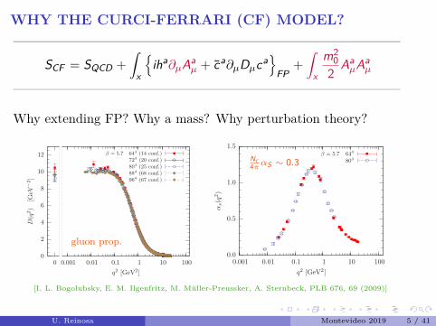
WHY THE CURCI-FERRARI (CF) MODEL?—————————————————————————————–

SCF = SQCD +

∫x

{iha∂µAa

µ + ca∂µDµca}

FP+

∫x

m20

2 AaµAa

µ

—————————————————————————————–

Why extending FP? Why a mass? Why perturbation theory?

0.001 0.01 0.1 1 10 100

q2 [GeV2]

β = 5.7 644 (14 conf.)724 (20 conf.)804 (25 conf.)884 (68 conf.)964 (67 conf.)

0

2

4

6

8

10

12

0

D(q

2)

[GeV

−2]

0.0

0.5

1.0

1.5

0.001 0.01 0.1 1 10 100

αs(q

2)

q2 [GeV2]

β = 5.7 644

804

gluon prop.

Nc4παS ∼ 0.3

[I. L. Bogolubsky, E. M. Ilgenfritz, M. Muller-Preussker, A. Sternbeck, PLB 676, 69 (2009)]


RATHER GOOD MODEL IN THE VACUUM

0 2 4 60.0

0.5

1.0

1.5

2.0

p HGeVL

p2GHpL

IS one - loop results

IS two - loop results

0 2 4 6

1.0

1.5

2.0

2.5

3.0

p HGeVL

FHpL

IS one - loop results

IS two - loop results

0.001 0.01 0.1 1 10 1000.0

0.5

1.0

1.5

Μ2HGeV

2L

ΑSHΜ

2L

reveal in the next talk

stay tuned!

[Plots from the pCF collaboration — Data from O. Oliveira et. al.]


FINITE TEMPERATURE EXTENSION?

What has the perturbative CF model to tell us regardingthe confinement/deconfinement transition?

phys.point

00

N = 2

N = 3

N = 1

f

f

f

m s

sm

Gauge

m , mu

1st

2nd orderO(4) ?

chiral2nd orderZ(2)

deconfined2nd orderZ(2)

crossover

1st

d

tric

∞

∞

Pure


FINITE TEMPERATURE EXTENSION?

What has the perturbative CF model to tell us regardingthe confinement/deconfinement transition?

0

0.2

0.4

0.6

0.8

1

1.2

0.5 1 1.5 2 2.5 3 3.5 4

Lren

T/Tc

Nf=2 m/T=0.40 Nt=4

Nf=0 Nt=4

Nf=0 Nt=8

phys.point

00

N = 2

N = 3

N = 1

f

f

f

m s

sm

Gauge

m , mu

1st

2nd orderO(4) ?

chiral2nd orderZ(2)


crossover

1st

d

tric

∞

∞

Pure


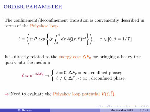
ORDER PARAMETER

The confinement/deconfinement transition is conveniently described interms of the Polyakov loop

` ≡⟨

tr P exp{

ig∫ β

0dτ Aa

0(τ,~x)ta}⟩

, τ ∈ [0, β = 1/T ]

It is directly related to the energy cost ∆Fq for bringing a heavy testquark into the medium

` ∝ e−β∆Fq →{` = 0,∆Fq =∞ : confined phase;` 6= 0,∆Fq <∞ : deconfined phase.

⇒ Need to evaluate the Polyakov loop potential V (`, ¯).


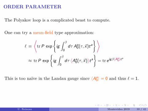
ORDER PARAMETER

The Polyakov loop is a complicated beast to compute.

One can try a mean-field type approximation:

` ≡⟨

tr P exp{

ig∫ β

0dτ Aa

0(τ,~x)ta}⟩

≈ tr P exp{

ig∫ β

0dτ⟨Aa

0(τ,~x)⟩ta}

= tr eigβ〈Aa0〉ta

This is too naıve in the Landau gauge since 〈Aa0〉 = 0 and thus ` = 1.


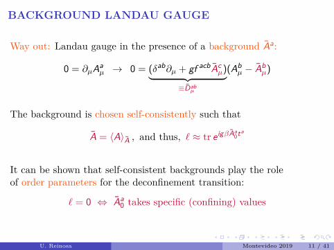
BACKGROUND LANDAU GAUGE

Way out: Landau gauge in the presence of a background Aa:

0 = ∂µAaµ → 0 = (δab∂µ + gf acbAc

µ)︸︷︷︸≡Dab

µ

(Abµ − Ab

µ)

The background is chosen self-consistently such that

A = 〈A〉A , and thus, ` ≈ tr eigβAa0ta

It can be shown that self-consistent backgrounds play the roleof order parameters for the deconfinement transition:

` = 0 ⇔ Aa0 takes specific (confining) values


BACKGROUND LANDAU GAUGE

—————————————————————————————–

SbgCF = SQCD +

∫x

{ihaDµAa

µ + caDµDµca}

bgFP+

∫x

m20

2 (Aaµ − Aa

µ)2

—————————————————————————————–

Self-consistent backgrounds are determined from the minimizationof a background effective action:

Γ[A] ≡ ΓA[A = A]

At finite T , one can restrict to backgrounds of the form

gβAa0ta = r3

λ32 + r8

λ82

We are then left with the minimization of a potential W (r3, r8)tantamount to V (`, ¯).


YANG-MILLS PHASE STRUCTURE

FROM PERTURBATIVE METHODS


ONE-LOOP BG POTENTIAL FROM THE CF MODEL

` ' tr eigβA0 , gβA0 = r3λ32 + r8

λ82

0 2 Π

3

4 Π

3

2 Π

0

V (`) = W (r3, r8 = 0)

` 6= 0↓

← ` = 0

[UR, J. Serreau, M. Tissier, N. Wschebor, PLB 742, 61 (2015)]


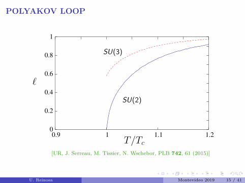
POLYAKOV LOOP

0

0.2

0.4

0.6

0.8

1

0.9 1 1.1 1.2

ℓ

T/Tc

SU(2)

SU(3)

[UR, J. Serreau, M. Tissier, N. Wschebor, PLB 742, 61 (2015)]


CONFINEMENT MECHANISMTake SU(2) for instance:

WSU(2)(r3) =3Tπ2

∫ ∞0

dq q2 Re ln(

1− e−β√

q2+m2+ir3)

massive gluons

− Tπ2

∫ ∞0

dq q2 Re ln(1− e−βq+ir3 ) massless ghosts

T � m :

2Tπ2

∫ ∞0

dq q2 Re ln(1− e−βq+ir3 )

T � m :

− Tπ2

∫ ∞0

dq q2 Re ln(1−e−βq+ir3 )

0 Π 2 Π

0

← `=0

This mechanism is common to most continuum approaches (fRG, . . . )and is rooted in the properties of the decoupling solution.


SUMMARY OF RESULTS (ONE-LOOP CF)

order lattice fRG CF model at 1-loopSU(2) 2nd 2nd 2ndSU(3) 1st 1st 1stSU(4) 1st 1st 1stSp(2) 1st 1st 1st

Tc (MeV) lattice fRG(∗) CF at 1-loop(∗∗)

SU(2) 295 230 238SU(3) 270 275 185

(∗) L. Fister and J. M. Pawlowski, Phys.Rev. D88 (2013) 045010.(∗∗) UR, J. Serreau, M. Tissier and N. Wschebor, Phys.Lett. B742 (2015) 61-68.


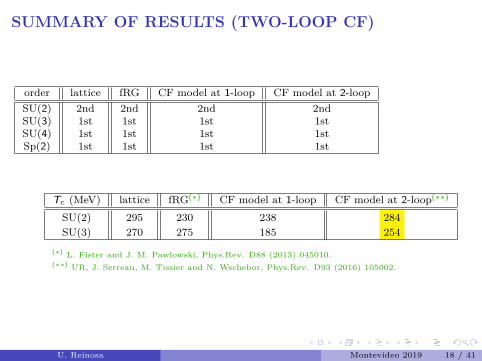
SUMMARY OF RESULTS (TWO-LOOP CF)

order lattice fRG CF model at 1-loop CF model at 2-loopSU(2) 2nd 2nd 2nd 2ndSU(3) 1st 1st 1st 1stSU(4) 1st 1st 1st 1stSp(2) 1st 1st 1st 1st

Tc (MeV) lattice fRG(∗) CF model at 1-loop CF model at 2-loop(∗∗)

SU(2) 295 230 238 284SU(3) 270 275 185 254

(∗) L. Fister and J. M. Pawlowski, Phys.Rev. D88 (2013) 045010.(∗∗) UR, J. Serreau, M. Tissier and N. Wschebor, Phys.Rev. D93 (2016) 105002.


HEAVY-QUARK QCD PHASE STRUCTURE

FROM PERTURBATIVE METHODS


COLUMBIA PLOT———————————————————————————————

· · ·+Nf∑

f =1

∫x

{ψf (∂/− igAa/ ta + Mf )ψf

},with Mf � T

———————————————————————————————

phys.point

00

N = 2

N = 3

N = 1

f

f

f

m s

sm

Gauge

m , mu

1st

2nd orderO(4) ?

chiral2nd orderZ(2)


crossover

1st

d

tric

∞

∞

Pure


COLUMBIA PLOT FROM THE CF MODEL

M > Mc :

2.8 3 3.2 3.4 3.6 3.8

V

r3

first order

M = Mc :

2.8 3 3.2 3.4 3.6 3.8

V

r3

second order

M < Mc :

2.8 3 3.2 3.4 3.6 3.8

V

r3

crossover


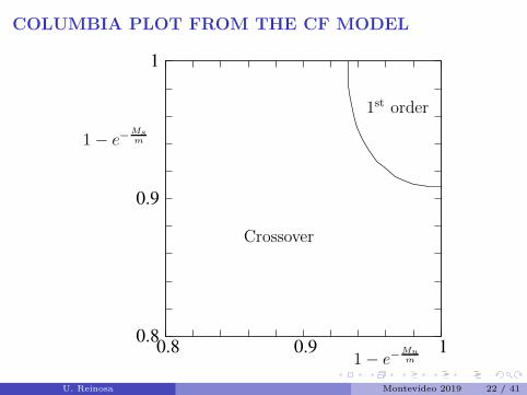
COLUMBIA PLOT FROM THE CF MODEL

1 0.9 0.8 0.8

0.9

1

Crossover

1st order

1− e−Msm

1− e−Mum


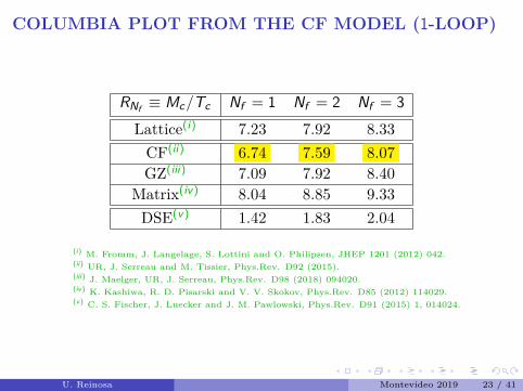
COLUMBIA PLOT FROM THE CF MODEL (1-LOOP)

RNf ≡ Mc/Tc Nf = 1 Nf = 2 Nf = 3Lattice(i) 7.23 7.92 8.33

CF(ii) 6.74 7.59 8.07GZ(iii) 7.09 7.92 8.40

Matrix(iv) 8.04 8.85 9.33DSE(v) 1.42 1.83 2.04

(i) M. Fromm, J. Langelage, S. Lottini and O. Philipsen, JHEP 1201 (2012) 042.(ii) UR, J. Serreau and M. Tissier, Phys.Rev. D92 (2015).(iii) J. Maelger, UR, J. Serreau, Phys.Rev. D98 (2018) 094020.(iv) K. Kashiwa, R. D. Pisarski and V. V. Skokov, Phys.Rev. D85 (2012) 114029.(v) C. S. Fischer, J. Luecker and J. M. Pawlowski, Phys.Rev. D91 (2015) 1, 014024.


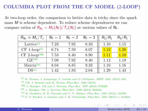
COLUMBIA PLOT FROM THE CF MODEL (2-LOOP)

At two-loop order, the comparison to lattice data is tricky since the quarkmass M is scheme dependent. To reduce scheme dependences we cancompare ratios of RNf = Mc(Nf )/Tc(Nf ) at various values of Nf .

RNf ≡ Mc/Tc Nf = 1 Nf = 2 Nf = 3 R2/R1 R3/R1

Lattice(i) 7.23 7.92 8.33 1.10 1.15CF 1-loop(ii) 6.74 7.59 8.07 1.12 1.20CF 2-loop(iib) 7.53 8.40 8.90 1.11 1.18

GZ(iii) 7.09 7.92 8.40 1.12 1.19Matrix(iv) 8.04 8.85 9.33 1.10 1.16

DS(v) 1.42 1.83 2.04 1.29 1.43

(i) M. Fromm, J. Langelage, S. Lottini and O. Philipsen, JHEP 1201 (2012) 042.(ii) UR, J. Serreau and M. Tissier, Phys.Rev. D92 (2015).(iib) J. Maelger, UR and J. Serreau, Phys.Rev. D97 (2018) 074027.(iii) J. Maelger, UR, J. Serreau, Phys.Rev. D98 (2018) 094020.(iv) K. Kashiwa, R. D. Pisarski and V. V. Skokov, Phys.Rev. D85 (2012) 114029.(v) C. S. Fischer, J. Luecker and J. M. Pawlowski, Phys.Rev. D91 (2015) 1, 014024.


IMAGINARY CHEMICAL POTENTIAL

———————————————————————————————

· · ·+Nf∑

f =1

∫x

{ψf (∂/− igAa/ ta + Mf − iµiγ0)ψf

},with Mf � T , µ

———————————————————————————————

Not really physical, but much praised by the lattice community sincethe sign problem is absent. For us, immense source of data to whichwe can compare to.

For µi = (π/3)T , the action admits a new symmetry (Roberge-Weiss),that combines center transformations, abelian gauge transformationsand charge conjugation.

The Roberge-Weiss (RW) symmetry is known to be broken for largeenough temperatures.


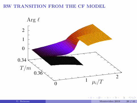
RW TRANSITION FROM THE CF MODEL

2

1

0

0.34

0.36 2

1 0

Arg ℓ

T/m

µi/T


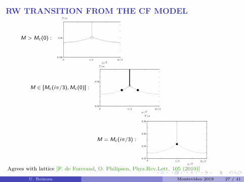
RW TRANSITION FROM THE CF MODEL

M > Mc (0) : 0.36

0.348

0 π/3 2π/3µi/T

T/m

M ∈ [Mc (iπ/3),Mc (0)] : 0.36

0.34

0µi/T

π/3 2π/3

T/m

M = Mc (iπ/3) :

0.38

0.36

0.34

0.32

µi/Tπ/3 2π/30

T/m

Agrees with lattice [P. de Forcrand, O. Philipsen, Phys.Rev.Lett. 105 (2010)]


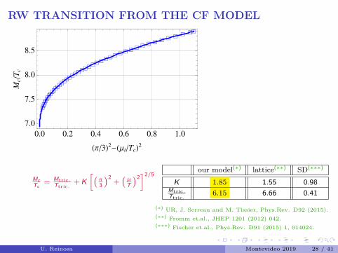
RW TRANSITION FROM THE CF MODEL��

0.0 0.2 0.4 0.6 0.8 1.0

7.0

7.5

8.0

8.5

HΠ�3L2-HΜi�TcL2

Mc�T

c

McTc

= Mtric.Ttric.

+ K[(

π3

)2+(µT

)2]2/5

our model(∗) lattice(∗∗) SD(∗∗∗)

K 1.85 1.55 0.98Mtric.Ttric.

6.15 6.66 0.41

(∗) UR, J. Serreau and M. Tissier, Phys.Rev. D92 (2015).(∗∗) Fromm et.al., JHEP 1201 (2012) 042.(∗∗∗) Fischer et.al., Phys.Rev. D91 (2015) 1, 014024.


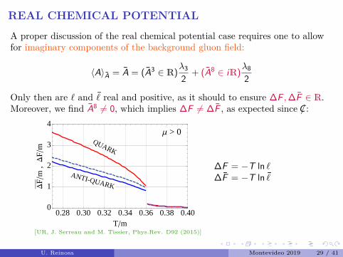
REAL CHEMICAL POTENTIAL

A proper discussion of the real chemical potential case requires one to allowfor imaginary components of the background gluon field:

〈A〉A = A = (A3 ∈ R)λ32 + (A8 ∈ iR)

λ82

Only then are ` and ¯ real and positive, as it should to ensure ∆F ,∆F ∈ R.Moreover, we find A8 6= 0, which implies ∆F 6= ∆F , as expected since /C :

Μ > 0QUARK

ANTI-QUARK

0.28 0.30 0.32 0.34 0.36 0.38 0.400

1

2

3

4

T�m

DF

�m,

DF

�m

∆F = −T ln `∆F = −T ln ¯

[UR, J. Serreau and M. Tissier, Phys.Rev. D92 (2015)]



A proper discussion of the real chemical potential case requires one to allowfor imaginary components of the background gluon field:

〈A〉A = A = (A3 ∈ R)λ32 + (A8 ∈ iR)

λ82

Only then are ` and ¯ real and positive, as it should to ensure ∆F ,∆F ∈ R.The µ-dependence is also in line with expectations:

∆Q = −T∂∆F/∂µ∆Q = −T∂∆F/∂µ

[J. Maelger, UR and J. Serreau, Phys.Rev. D97 (2018) 074027]



The critical line moves towards larger quark masses as µ is increased:

0.8

0.9

1

0.8 0.9 1

1− e−Msm

1− e−Mum

in full agreement with lattice simulations.


QCD PHASE DIAGRAM FROM

THE RAINBOW-IMPROVED EXPANSION


INFRARED COUPLINGS

For light quark masses, the quark-gluon vertex coupling gq(p) is up to2× larger in the infrared than the pure YM coupling gg (p):

0 1 2 3 4 5 60.5

1.0

1.5

2.0

2.5

p H GeV L

Λ1

HpL

Perturbation theory is not justified in this case.

[Skullerud et al, JHEP 0304 (2003) 047.]


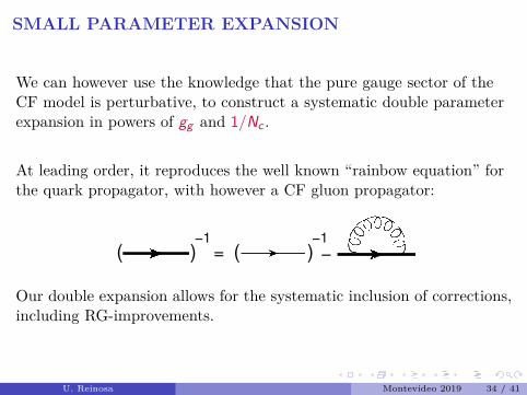
SMALL PARAMETER EXPANSION

We can however use the knowledge that the pure gauge sector of theCF model is perturbative, to construct a systematic double parameterexpansion in powers of gg and 1/Nc .

At leading order, it reproduces the well known “rainbow equation” forthe quark propagator, with however a CF gluon propagator:

=− 1

( ) −− 1

( )

Our double expansion allows for the systematic inclusion of corrections,including RG-improvements.


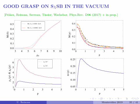
GOOD GRASP ON SχSB IN THE VACUUM

[Pelaez, Reinosa, Serreau, Tissier, Wschebor, Phys.Rev. D96 (2017) + in prep.]

3 4 5 6 7 8 9 10

0.0

0.1

0.2

0.3

0.4

0.5

g0

MH0L

M H L 1 L =0.0001 GeV

M H L 1 L =0.001 GeV

0 1 2 3 4 50.0

0.1

0.2

0.3

0.4

p

MHpL

0 1 2 3 4 51

2

3

4

5

6

p

ggHpL

&g

qHpL gq H p L

gg H p L

0 1 2 3 4 5

0.05

0.10

0.15

0.20

0.25

p

mHpL


PHASE DIAGRAM

[J. Maelger, UR, J. Serreau, arXiv:1903.04184.]


BOTTOM-LEFT CORNER OF THE COLUMBIA PLOT

Similar result as with quark-meson effective models at mean-field levelwithout anomaly, as expected in a leading order 1/Nc calculation.

phys.point

00

N = 2

N = 3

N = 1

f

f

f

m s

sm

Gauge

m , mu

1st

2nd orderO(4) ?

chiral2nd orderZ(2)


crossover

1st

d

tric

∞

∞

Pure

0

50

100

150 0100

200300

400500

600

100

200

300

µ [MeV]

mπ [MeV]mK [MeV]

µ [MeV]

2nd

crossover

1st

[S. Resch, F. Rennecke, B.-J. Schaefer, Phys.Rev. D99 (2019)]


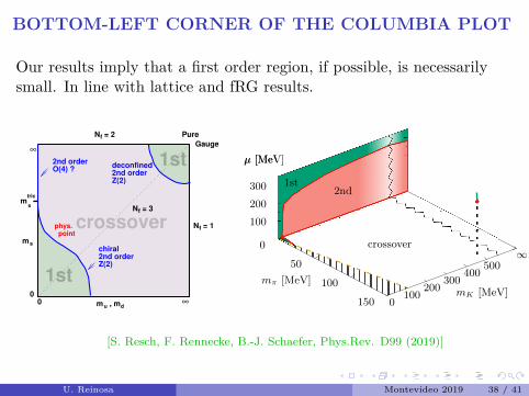
BOTTOM-LEFT CORNER OF THE COLUMBIA PLOT

Our results imply that a first order region, if possible, is necessarilysmall. In line with lattice and fRG results.

phys.point

00

N = 2

N = 3

N = 1

f

f

f

m s

sm

Gauge

m , mu

1st

2nd orderO(4) ?

chiral2nd orderZ(2)


crossover

1st

d

tric

∞

∞

Pure

0

50

100

150 0100

200300

400500

∞

100

200

300

µ [MeV]

mπ [MeV]mK [MeV]

µ [MeV]

2nd1st

crossover

[S. Resch, F. Rennecke, B.-J. Schaefer, Phys.Rev. D99 (2019)]


INTERPLAY WITH THE DECONFINEMENTTRANSITION

[J. Maelger, UR, J. Serreau, in preparation.]


CONCLUSIONS

In the Landau gauge, the Faddeev-Popov action is not a faithful descriptionof Yang-Mills theory at low energies.

A simple model beyond the Faddeev-Popov recipe seems to renderperturbation theory viable at all scales (in YM theory/heavy QCD):

∗ Lattice correlators are reproduced quite satisfactorily at LO.

∗ The phase structure of pure Yang-Mills is reproduced.

∗ This applies also to QCD in the heavy-quark limit.

∗ Two-loop corrections improve the results.

Perturbation theory is not applicable in the presence of light quarks buta double parameter expansion in powers of gg and 1/Nc gives a goodaccount of chiral symmetry breaking already at leading order.

Preliminary results at finite temperature are also promising.


THANK YOU ALLFOR YOUR ATTENTION!


QCD AT FINITE TEMPERATURE AND DENSITY FROM THE CURCI ...

Documents

Transcript of QCD AT FINITE TEMPERATURE AND DENSITY FROM THE CURCI ...