Python And Performance

Chris MyersCenter for Advanced Computing

and Department of Physics / Laboratory of Atomic & Solid State PhysicsCornell University

1 Introduction

• Python is interpreted: Python source code is executed by a program known as an interpreter• In compiled languages (e.g., C/C++, Fortran), source code is compiled to an executable pro-

gram• Compiled programs generally run faster than interpreted programs• Interpreted languages are often better for rapid prototyping and high-level program control• Optimizing “time to science” might suggest prioritizing program development time over

computational run time (or maybe vice versa)• Python has become a popular language for scientific computing for many reasons

• How should we best use Python for applications that require numerically intensive compu-tations?

• Can we have the best of both worlds (expressiveness and performance)?• If there are tradeoffs, where are they and how can they be mitigated?• As with most things in Python, there is no one answer. . .

2 CPython and the Python/C API

• CPython: the reference implementation of the language, and the most widely used inter-preter (generally installed as “python”)

• Alternative implementations/interpreters exist (e.g., IronPython, Jython, PyPy) — we willnot consider these here

• IPython & Jupyter kernel are thin Python layers on top of CPython to provide additionalfunctionality

– but typically use python myprogram.py for long-running programs in batch• CPython compiles Python source code to bytecodes, and then operates on those• CPython, written in C, is accompanied by an Application Programming Interface (API) that

enables communication between Python and C (and thus to basically any other language)• Python/C API allows for compiled chunks of code to be called from Python or executed

within the CPython interpreter → extension modules• Much core functionality of the Python language and standard library are written in C

1

3 Extension Modules

• a compiled shared object library (.so, .dll, etc.) making use of Python/C API– compiled code executing operations of interest– wrapper/interface code consisting of calls to Python/C API and underlying compiled

code• can be imported into python interpreter just as pure Python source code can

3.1 Extension modules

[1]: import mathprint(math.cos(math.pi))

print(math.__file__)

-1.0/Users/myers/anaconda3/envs/work/lib/python3.7/lib-dynload/math.cpython-37m-darwin.so

[2]: !nm $math.__file__

U _PyArg_ParseU _PyArg_ParseTupleU _PyArg_UnpackTupleU _PyBool_FromLongU _PyErr_ClearU _PyErr_ExceptionMatchesU _PyErr_FormatU _PyErr_OccurredU _PyErr_SetFromErrnoU _PyErr_SetStringU _PyExc_MemoryErrorU _PyExc_OverflowErrorU _PyExc_TypeErrorU _PyExc_ValueErrorU _PyFloat_AsDoubleU _PyFloat_FromDoubleU _PyFloat_Type

00000000000012f0 T _PyInit_mathU _PyIter_NextU _PyLong_AsDoubleU _PyLong_AsLongAndOverflowU _PyLong_FromDoubleU _PyLong_FromLongU _PyLong_FromUnsignedLongU _PyMem_FreeU _PyMem_MallocU _PyMem_Realloc

2

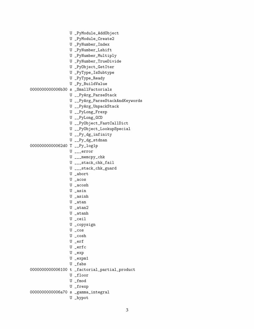
U _PyModule_AddObjectU _PyModule_Create2U _PyNumber_IndexU _PyNumber_LshiftU _PyNumber_MultiplyU _PyNumber_TrueDivideU _PyObject_GetIterU _PyType_IsSubtypeU _PyType_ReadyU _Py_BuildValue

0000000000006b30 s _SmallFactorialsU __PyArg_ParseStackU __PyArg_ParseStackAndKeywordsU __PyArg_UnpackStackU __PyLong_FrexpU __PyLong_GCDU __PyObject_FastCallDictU __PyObject_LookupSpecialU __Py_dg_infinityU __Py_dg_stdnan

00000000000062d0 T __Py_log1pU ___errorU ___memcpy_chkU ___stack_chk_failU ___stack_chk_guardU _abortU _acosU _acoshU _asinU _asinhU _atanU _atan2U _atanhU _ceilU _copysignU _cosU _coshU _erfU _erfcU _expU _expm1U _fabs

0000000000006100 t _factorial_partial_productU _floorU _fmodU _frexp

0000000000006a70 s _gamma_integralU _hypot

3

0000000000006a00 s _lanczos_den_coeffs0000000000006990 s _lanczos_num_coeffs

U _ldexpU _logU _log10U _log1pU _log2

0000000000005d50 t _loghelper00000000000061f0 t _m_atan20000000000006070 t _m_log0000000000005fe0 t _m_log100000000000005cd0 t _m_log20000000000005980 t _m_remainder0000000000005ea0 t _math_10000000000005ad0 t _math_200000000000013c0 t _math_acos0000000000007960 d _math_acos_doc0000000000001500 t _math_acosh00000000000079b0 d _math_acosh_doc0000000000001640 t _math_asin0000000000007a00 d _math_asin_doc0000000000001780 t _math_asinh0000000000007a50 d _math_asinh_doc00000000000018c0 t _math_atan0000000000001a00 t _math_atan20000000000007af0 d _math_atan2_doc0000000000007aa0 d _math_atan_doc0000000000001a20 t _math_atanh0000000000007b80 d _math_atanh_doc0000000000001b60 t _math_ceil0000000000008da8 d _math_ceil.PyId___ceil__0000000000007bd0 d _math_ceil__doc__0000000000001d10 t _math_copysign0000000000007c40 d _math_copysign_doc0000000000001d30 t _math_cos0000000000007d00 d _math_cos_doc0000000000001e70 t _math_cosh0000000000007d50 d _math_cosh_doc0000000000001fa0 t _math_degrees0000000000007d90 d _math_degrees__doc__0000000000002010 t _math_erf0000000000007de0 d _math_erf_doc00000000000020f0 t _math_erfc0000000000007e10 d _math_erfc_doc00000000000021d0 t _math_exp0000000000007e50 d _math_exp_doc0000000000002300 t _math_expm10000000000007e90 d _math_expm1_doc

4

0000000000002430 t _math_fabs0000000000007f30 d _math_fabs_doc0000000000002560 t _math_factorial0000000000007f80 d _math_factorial__doc__0000000000002920 t _math_floor0000000000008d90 d _math_floor.PyId___floor__0000000000007fe0 d _math_floor__doc__0000000000002ad0 t _math_fmod0000000000008050 d _math_fmod__doc__0000000000002c60 t _math_frexp00000000000080b0 d _math_frexp__doc__0000000000002d10 t _math_fsum0000000000008180 d _math_fsum__doc__0000000000003230 t _math_gamma0000000000008210 d _math_gamma_doc0000000000003a50 t _math_gcd0000000000008240 d _math_gcd__doc__0000000000003b40 t _math_hypot0000000000008280 d _math_hypot__doc__0000000000003cf0 t _math_isclose00000000000072a0 s _math_isclose._keywords0000000000008d50 d _math_isclose._parser00000000000082d0 d _math_isclose__doc__0000000000003e60 t _math_isfinite0000000000008590 d _math_isfinite__doc__0000000000003ee0 t _math_isinf0000000000008600 d _math_isinf__doc__0000000000003f60 t _math_isnan0000000000008670 d _math_isnan__doc__0000000000003fd0 t _math_ldexp00000000000086d0 d _math_ldexp__doc__0000000000004210 t _math_lgamma0000000000008730 d _math_lgamma_doc00000000000046a0 t _math_log0000000000004d50 t _math_log1000000000000088b0 d _math_log10__doc__0000000000004c00 t _math_log1p0000000000008820 d _math_log1p_doc0000000000004d70 t _math_log200000000000088f0 d _math_log2__doc__0000000000008790 d _math_log__doc__00000000000073a0 d _math_methods0000000000004d90 t _math_modf0000000000008930 d _math_modf__doc__0000000000004e60 t _math_pow00000000000089b0 d _math_pow__doc__0000000000005220 t _math_radians00000000000089f0 d _math_radians__doc__

5

0000000000005290 t _math_remainder0000000000008a40 d _math_remainder_doc00000000000052b0 t _math_sin0000000000008b60 d _math_sin_doc00000000000053f0 t _math_sinh0000000000008bb0 d _math_sinh_doc0000000000005520 t _math_sqrt0000000000008bf0 d _math_sqrt_doc0000000000005660 t _math_tan0000000000008c30 d _math_tan_doc00000000000057a0 t _math_tanh0000000000008c80 d _math_tanh_doc00000000000058e0 t _math_trunc0000000000008d38 d _math_trunc.PyId___trunc__0000000000008cc0 d _math_trunc__doc__00000000000072d0 d _mathmodule

U _memcpyU _modf

0000000000007340 d _module_docU _powU _roundU _sinU _sinhU _sqrtU _tanU _tanhU dyld_stub_binder

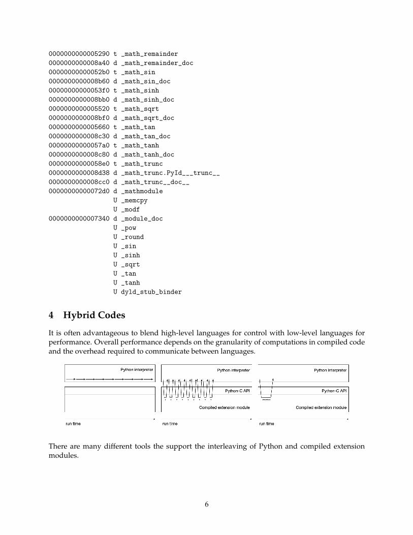
4 Hybrid Codes

It is often advantageous to blend high-level languages for control with low-level languages forperformance. Overall performance depends on the granularity of computations in compiled codeand the overhead required to communicate between languages.

There are many different tools the support the interleaving of Python and compiled extensionmodules.

6

5 Comments and caveats about performance optimization

• Make sure you have the right algorithm for the task at hand• Remember that “premature optimization is the root of all evil” (D. Knuth)• Focus on performance optimization only for those pieces of code that need it• Algorithms and computational architectures are complex: be empirical about performance

6 Outline

• Introduction• Leveraging Compiled Code

– Compiled Third-Party Libraries– Compiling Custom Code

• Leveraging Additional Computational Resources– Parallel Processing

• Writing Faster Python• Performance Assessment

Material derived in part from Cornell Virtual Workshop (CVW) tutorial on “Python for High Per-formance”, at https://cvw.cac.cornell.edu/python .

These slides will be available as a Jupyter notebook linked from the CVW site. Note: some codepresented here is in the form of incomplete snippets to illustrate a point. This notebook willtherefore not run from start to finish without errors.

7 Third-Party Libraries for Numerical & Scientific Computing

a.k.a. The Python Scientific Computing Ecosystem

• Most specific functionality for scientific computing is provided by third-party libraries,which are typically a mix of Python code and compiled extension modules

– NumPy: multi-dimensional arrays and array operations, linear algebra, random num-bers

– SciPy: routines for integration, optimization, root-finding, interpolation, fitting, etc.– Pandas: Series and Dataframes to handle tabular data (e.g., from spreadsheets)– Scikit-learn, TensorFlow, Caffe, PyTorch, Keras: machine learning– NetworkX: networks– Matplotlib, Seaborn: plotting– etc.

• Bundled distributions (e.g, Anaconda) contain many of these, with tools for installing addi-tional packages

8 NumPy

• NumPy = “Numerical Python”, the cornerstone of the Python Scientific Computing Ecosys-tem

• largely written in C, with links to BLAS and LAPACK for linear algebra• provides multidimensional arrays and array-level operations (a form of vectorization)

7

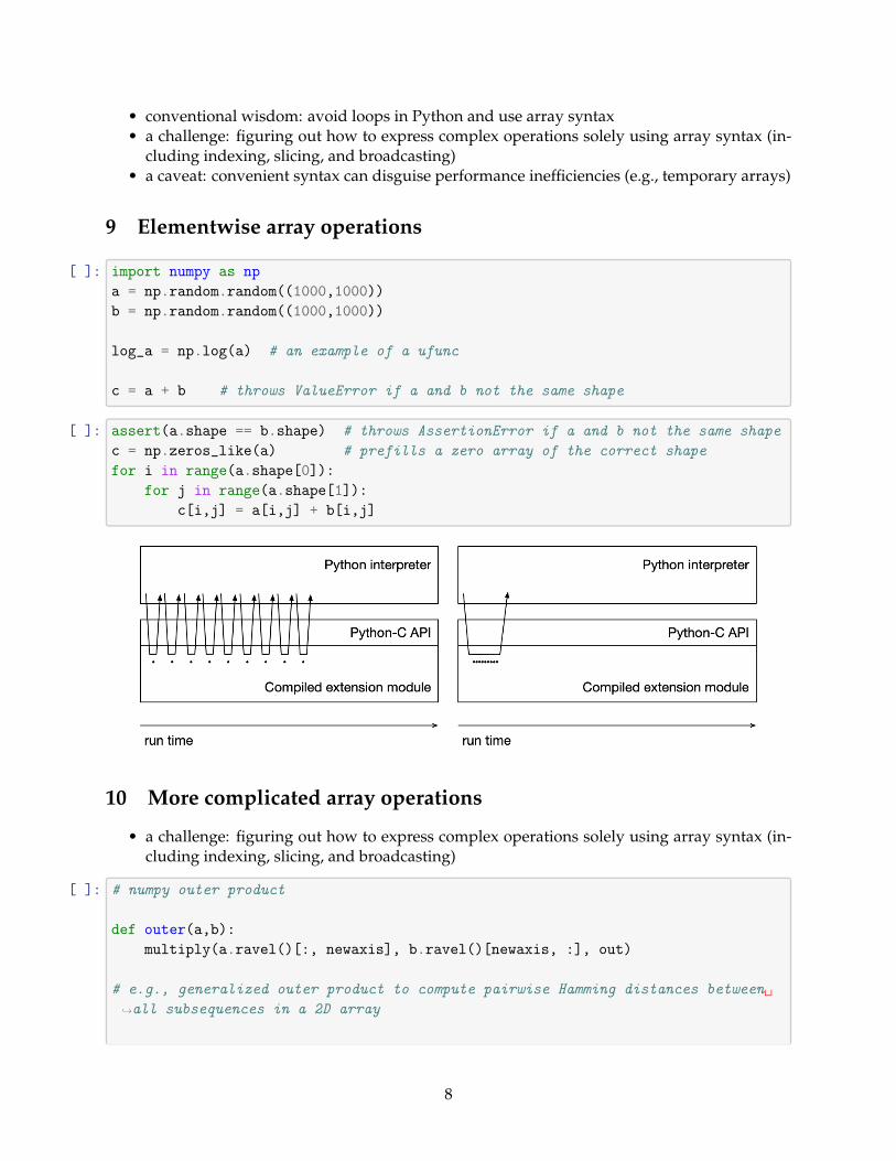
• conventional wisdom: avoid loops in Python and use array syntax• a challenge: figuring out how to express complex operations solely using array syntax (in-

cluding indexing, slicing, and broadcasting)• a caveat: convenient syntax can disguise performance inefficiencies (e.g., temporary arrays)

9 Elementwise array operations

[ ]: import numpy as npa = np.random.random((1000,1000))b = np.random.random((1000,1000))

log_a = np.log(a) # an example of a ufunc

c = a + b # throws ValueError if a and b not the same shape

[ ]: assert(a.shape == b.shape) # throws AssertionError if a and b not the same shapec = np.zeros_like(a) # prefills a zero array of the correct shapefor i in range(a.shape[0]):

for j in range(a.shape[1]):c[i,j] = a[i,j] + b[i,j]

10 More complicated array operations

• a challenge: figuring out how to express complex operations solely using array syntax (in-cluding indexing, slicing, and broadcasting)

[ ]: # numpy outer product

def outer(a,b):multiply(a.ravel()[:, newaxis], b.ravel()[newaxis, :], out)

# e.g., generalized outer product to compute pairwise Hamming distances between␣↪→all subsequences in a 2D array

8

def Hamming_outer(a0,a1):return np.sum(np.bitwise_xor(a0[:,np.newaxis], a1[np.newaxis,:]), axis=2)

11 More complicated array operations

[ ]: # e.g., approximate Laplacian on 2D array by summing up shifted copies of array

def Del2(a, dx):nx, ny = a.shapedel2a = scipy.zeros((nx, ny), float)del2a[1:-1, 1:-1] = (a[1:-1,2:] + a[1:-1,:-2] + \

a[2:,1:-1] + a[:-2,1:-1] - 4.*a[1:-1,1:-1])/(dx*dx)return del2a

# roughly equivalent to:

for i in range(1,nx-1):for j in range(1,ny-1):

del2a[i,j] = (a[i+1,j] + a[i-1,j] + a[i,j+1] + a[i,j-1] - 4*a[i,j])/↪→(dx*dx)

12 NumPy and optimized libraries

• NumPy performance can be enhanced if linked to optimized libraries– numpy.__config__.show() to list what blas, lapack libraries numpy is linked to

• Intel MKL (Math Kernel Library) is highly optimized for Intel processors, and bundled withAnaconda Python distribution

• On multi-core architectures, optimized libraries can provide NumPy-based parallelism forfree by setting environment variables appropriate for processor

– MKL_NUM_THREADS = N # if using MKL– OMP_NUM_THREADS = N # if libraries support OpenMP

13 NumPy and temporary array creation

∂u∂t

= D∇2u + u(1− u)

[ ]: u += dt * ( D * Del2(u) + u * (1 - u) )

Temporary arrays created: * Del2(u) * D * Del2(u) * 1 - u * u * (1 - u) * D * Del2(u) + u * (1 - u) * dt *( D * Del2(u) + u * (1 - u) )

9

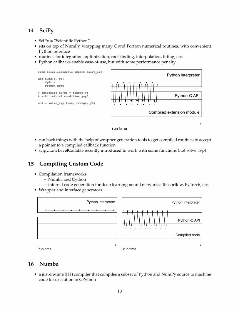
14 SciPy

• SciPy = “Scientific Python”• sits on top of NumPy, wrapping many C and Fortran numerical routines, with convenient

Python interface• routines for integration, optimization, root-finding, interpolation, fitting, etc.• Python callbacks enable ease-of-use, but with some performance penalty

• can hack things with the help of wrapper generation tools to get compiled routines to accepta pointer to a compiled callback function

• scipy.LowLevelCallable recently introduced to work with some functions (not solve_ivp)

15 Compiling Custom Code

• Compilation frameworks– Numba and Cython– internal code generation for deep learning neural networks: Tensorflow, PyTorch, etc.

• Wrapper and interface generators

16 Numba

• a just-in-time (JIT) compiler that compiles a subset of Python and NumPy source to machinecode for execution in CPython

10

• uses LLVM to convert Python bytecodes to intermediate representation (IR), and generatesoptimizes C code from that

• can be configured in more detail, but some performance improvements simply via additionof @jit decorator

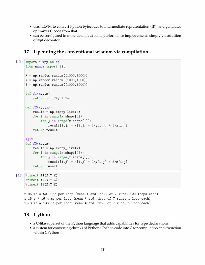
17 Upending the conventional wisdom via compilation

[3]: import numpy as npfrom numba import jit

X = np.random.random((1000,1000))Y = np.random.random((1000,1000))Z = np.random.random((1000,1000))

def f1(x,y,z):return x + 2*y + 3*z

def f2(x,y,z):result = np.empty_like(x)for i in range(x.shape[0]):

for j in range(x.shape[1]):result[i,j] = x[i,j] + 2*y[i,j] + 3*z[i,j]

return result

@jitdef f3(x,y,z):

result = np.empty_like(x)for i in range(x.shape[0]):

for j in range(x.shape[1]):result[i,j] = x[i,j] + 2*y[i,j] + 3*z[i,j]

return result

[4]: %timeit f1(X,Y,Z)%timeit f2(X,Y,Z)%timeit f3(X,Y,Z)

2.96 ms ± 50.9 µs per loop (mean ± std. dev. of 7 runs, 100 loops each)1.15 s ± 16.4 ms per loop (mean ± std. dev. of 7 runs, 1 loop each)1.73 ms ± 133 µs per loop (mean ± std. dev. of 7 runs, 1 loop each)

18 Cython

• a C-like superset of the Python language that adds capabilities for type declarations• a system for converting chunks of Python/Cython code into C for compilation and exeuction

within CPython

11

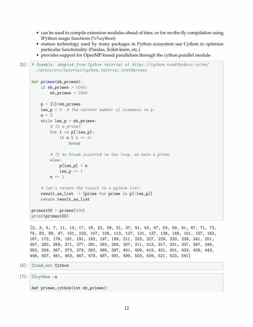
• can be used to compile extension modules ahead of time, or for on-the-fly compilation usingIPython magic functions (%%cython)

• mature technology used by many packages in Python ecosystem use Cython to optimizeparticular functionality (Pandas, Scikit-learn, etc.)

• provides support for OpenMP-based parallelism through the cython.parallel module

[5]: # Example: adapted from Cython tutorial at https://cython.readthedocs.io/en/↪→latest/src/tutorial/cython_tutorial.html#primes

def primes(nb_primes):if nb_primes > 1000:

nb_primes = 1000

p = [0]*nb_primeslen_p = 0 # The current number of elements in p.n = 2while len_p < nb_primes:

# Is n prime?for i in p[:len_p]:

if n % i == 0:break

# If no break occurred in the loop, we have a prime.else:

p[len_p] = nlen_p += 1

n += 1

# Let's return the result in a python list:result_as_list = [prime for prime in p[:len_p]]return result_as_list

primes100 = primes(100)print(primes100)

[2, 3, 5, 7, 11, 13, 17, 19, 23, 29, 31, 37, 41, 43, 47, 53, 59, 61, 67, 71, 73,79, 83, 89, 97, 101, 103, 107, 109, 113, 127, 131, 137, 139, 149, 151, 157, 163,167, 173, 179, 181, 191, 193, 197, 199, 211, 223, 227, 229, 233, 239, 241, 251,257, 263, 269, 271, 277, 281, 283, 293, 307, 311, 313, 317, 331, 337, 347, 349,353, 359, 367, 373, 379, 383, 389, 397, 401, 409, 419, 421, 431, 433, 439, 443,449, 457, 461, 463, 467, 479, 487, 491, 499, 503, 509, 521, 523, 541]

[6]: %load_ext Cython

[7]: %%cython -a

def primes_cython(int nb_primes):

12

cdef int n, i, len_pcdef int p[1000]if nb_primes > 1000:

nb_primes = 1000

len_p = 0 # The current number of elements in p.n = 2while len_p < nb_primes:

# Is n prime?for i in p[:len_p]:

if n % i == 0:break

# If no break occurred in the loop, we have a prime.else:

p[len_p] = nlen_p += 1

n += 1

# Let's return the result in a python list:result_as_list = [prime for prime in p[:len_p]]return result_as_list

cprimes100 = primes_cython(100)print(cprimes100)

[2, 3, 5, 7, 11, 13, 17, 19, 23, 29, 31, 37, 41, 43, 47, 53, 59, 61, 67, 71, 73,79, 83, 89, 97, 101, 103, 107, 109, 113, 127, 131, 137, 139, 149, 151, 157, 163,167, 173, 179, 181, 191, 193, 197, 199, 211, 223, 227, 229, 233, 239, 241, 251,257, 263, 269, 271, 277, 281, 283, 293, 307, 311, 313, 317, 331, 337, 347, 349,353, 359, 367, 373, 379, 383, 389, 397, 401, 409, 419, 421, 431, 433, 439, 443,449, 457, 461, 463, 467, 479, 487, 491, 499, 503, 509, 521, 523, 541]

[7]: <IPython.core.display.HTML object>Cython output in Jupyter shows annotated verson of code, which can be clicked on␣

↪→to reveal injected C code

[8]: %timeit primes(100)

%timeit primes_cython(100)

367 µs ± 1.15 µs per loop (mean ± std. dev. of 7 runs, 1000 loops each)18.8 µs ± 21.8 ns per loop (mean ± std. dev. of 7 runs, 100000 loops each)

13

19 Wrapper and Interface Generators

Useful if you have an existing code base (C/C++, Fortran, etc.) that you would like to be able tocall from Python

Typically a multi-step process:

• Python/C API code generation from function and class declarations

• wrapper code compiled and linked with underlying library → .so file

• possibly some additional Python code generated

Some of the many packages available:

• CFFI and ctypes provide "foreign function interfaces", or lightweight APIs, for calling Clibraries from within Python

• Boost.python helps write C++ libraries that Python can import

• SWIG reads C and C++ header files and generates a library than Python (or many otherscripting languages) can import

• F2PY reads Fortran code and generates a library that Python can import

• PyCUDA and PyOpenCL provide access within Python to GPUs

20 Parallel Processing

• Parallelization: across threads, across cores, across processors– . . . to reduce wallclock time to solution– . . . to solve bigger problems that don’t fit in a single processor

• CPython uses Global Interpreter Lock (GIL): only one thread can run at a time• GIL does not apply to multithreaded code in compiled library (e.g., MKL)• Multiple Python processes can run concurrently (each with their own GIL)• (and new development is apparently underway to enable multiple interpreters within a sin-

gle process)

14

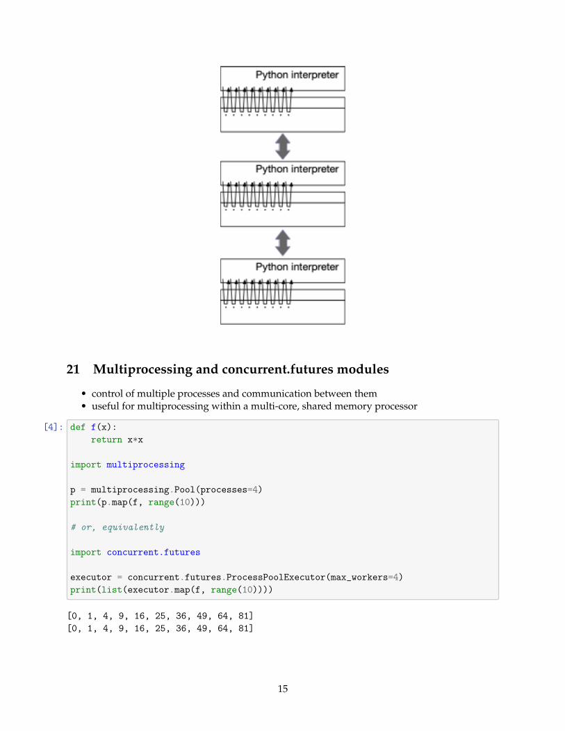
21 Multiprocessing and concurrent.futures modules

• control of multiple processes and communication between them• useful for multiprocessing within a multi-core, shared memory processor

[4]: def f(x):return x*x

import multiprocessing

p = multiprocessing.Pool(processes=4)print(p.map(f, range(10)))

# or, equivalently

import concurrent.futures

executor = concurrent.futures.ProcessPoolExecutor(max_workers=4)print(list(executor.map(f, range(10))))

[0, 1, 4, 9, 16, 25, 36, 49, 64, 81][0, 1, 4, 9, 16, 25, 36, 49, 64, 81]

15

22 More multiprocessing (from networkx docs)

Link to networkx page

[ ]: # just a subset of the code (download full example at link above to run)

def _betmap(G_normalized_weight_sources_tuple):return nx.betweenness_centrality_source(*G_normalized_weight_sources_tuple)

def betweenness_centrality_parallel(G, processes=None):"""Parallel betweenness centrality function"""p = Pool(processes=processes)node_divisor = len(p._pool) * 4node_chunks = list(chunks(G.nodes(), int(G.order() / node_divisor)))num_chunks = len(node_chunks)bt_sc = p.map(_betmap,

zip([G] * num_chunks,[True] * num_chunks,[None] * num_chunks,node_chunks))

# Reduce the partial solutionsbt_c = bt_sc[0]for bt in bt_sc[1:]:

for n in bt:bt_c[n] += bt[n]

return bt_c

23 Message passing with mpi4py

• MPI = “Message Passing Interface” — a widely-used standard for parallel processing• Many Python wrappers to MPI developed over the years; mpi4py is probably most widely

used at this time• use mpiexec or ibrun in shell to run a python program over multiple processors

– e.g., ibrun python myprogram.py on Stampede2 at TACC

23.1 mpi4py

[5]: from mpi4py import MPIcomm = MPI.COMM_WORLDprint(comm.Get_rank())print(comm.Get_size())

import numpy as npdata = np.arange(1000, dtype=np.float64)data2 = np.zeros(1000, dtype=np.float64)print(data2[:5])

16

comm.Isend(data, dest=0, tag=20)comm.Recv(data2, source=0, tag=20)print(data2[:5])

01[0. 0. 0. 0. 0.][0. 1. 2. 3. 4.]

24 Exercise: Estimating π via Monte Carlo using mpi4py

Exercise in CVW on “Python for High Performance”

25 Other Parallel Tools

• Dask– distributed NumPy arrays and Pandas DataFrames– task scheduling interface for custom workflows

• Joblib– lightweight pipelining with support for parallel processing– specific optimizations for NumPy arrays

• ipyparallel– parallel and distributed computing within IPython

26 Writing Faster Python

• Collections and containers• Lazy evaluation• Memory management

26.1 Collections and containers

Use the right data structure for the job

[1]: set1 = set(range(0,1000)) # create a set with a bunch of numbers in itset2 = set(range(500,2000)) # create another set with a bunch of numbers in␣

↪→itisec = set1 & set2 # same as isec = set1.intersection(set2)

list1 = list(range(0,1000)) # create a list with a bunch of numbers in itlist2 = list(range(500,2000)) # create another list with a bunch of numbers in␣

↪→itisec = [e1 for e1 in list1 for e2 in list2 if e1==e2] # uses list␣

↪→comprehensions

17

%timeit set1 & set2%timeit [e1 for e1 in list1 for e2 in list2 if e1==e2]

14.3 µs ± 92.7 ns per loop (mean ± std. dev. of 7 runs, 100000 loops each)35.3 ms ± 610 µs per loop (mean ± std. dev. of 7 runs, 10 loops each)

26.2 Lazy evaluation

• a strategy implemented in some programming languages whereby certain objects are notproduced until they are needed

• often used in conjunction with functions that produce collections of objects• if you only need to iterate over the items in a collection, you don’t need to produce that

entire collection

Python provides a variety of mechanisms to support lazy evaluation:

• generators: like functions, but maintain internal state and yield next value when called• dictionary views (keys and values)• range: for i in range(N)• zip: pairs = zip(seq1, seq2)• enumerate: for i, val in enumerate(seq)• open: with open(filename, 'r') as f

27 Performance Assessment

• Timing: getting timing information for particular operations• Profiling: figuring out where time is being spent

IPython magic functions

• %timeit : uses timeit module from Python Standard Library• %prun : uses profile module from Python Standard Library

[7]: from scipy.integrate import solve_ivp

sigma = 10rho = 28beta = 8.0/3

def lorenz(t, xyz):x,y,z = xyzxdot = sigma*(y-x)ydot = x*(rho-z) - yzdot = x*y - beta*zreturn [xdot, ydot, zdot]

def integrate_lorenz(ic=[1.,1.,1.]):sol = solve_ivp(lorenz, (0., 100.), ic, method='LSODA')return sol

18

%prun integrate_lorenz()

[5]: sol = integrate_lorenz()xs, ys, zs = sol['y']

[6]: import matplotlib.pyplot as pltfrom mpl_toolkits.mplot3d import Axes3D%matplotlib inlinefig = plt.figure(figsize=(10,8))ax = fig.gca(projection='3d')

ax.plot(xs, ys, zs, lw=0.5)ax.set_xlabel("X Axis")ax.set_ylabel("Y Axis")ax.set_zlabel("Z Axis")ax.set_title("I'll fly away");

19

28 Summary

• Python and Performance together in one big tent• There is no one answer: think about how you can best optimize “time to science”• Make sure you have the right algorithms, do not prematurely optimize, and be empirical

about performance

[ ]:

20