PYthon

Python for Informatics

Exploring Information

Version 2.7.0

Charles Severance

Copyright © 2009- Charles Severance.

Printing history:

May 2014: Editorial pass thanks to Sue Blumenberg.

October 2013: Major revision to Chapters 13 and 14 to switch to JSON and use OAuth.

Added new chapter on Visualization.

September 2013: Published book on Amazon CreateSpace

January 2010: Published book using the University of Michigan Espresso Book ma-

chine.

December 2009: Major revision to chapters 2-10 from Think Python: How to Think Like

a Computer Scientist and writing chapters 1 and 11-15 to produce Python for In-

formatics: Exploring Information

June 2008: Major revision, changed title to Think Python: How to Think Like a Com-

puter Scientist.

August 2007: Major revision, changed title to How to Think Like a (Python) Program-

mer.

April 2002: First edition of How to Think Like a Computer Scientist.

This work is licensed under a Creative Common Attribution-NonCommercial-ShareAlike

3.0 Unported License. This license is available at creativecommons.org/licenses/

by-nc-sa/3.0/. You can see what the author considers commercial and non-commercial

uses of this material as well as license exemptions in the Appendix titled Copyright Detail.

The LATEX source for the Think Python: How to Think Like a Computer Scientist version

of this book is available from http://www.thinkpython.com.

Preface

Python for Informatics: Remixing an Open Book

It is quite natural for academics who are continuously told to “publish or perish”

to want to always create something from scratch that is their own fresh creation.

This book is an experiment in not starting from scratch, but instead “remixing”

the book titled Think Python: How to Think Like a Computer Scientist written by

Allen B. Downey, Jeff Elkner, and others.

In December of 2009, I was preparing to teach SI502 - Networked Programming

at the University of Michigan for the fifth semester in a row and decided it was time

to write a Python textbook that focused on exploring data instead of understanding

algorithms and abstractions. My goal in SI502 is to teach people lifelong data

handling skills using Python. Few of my students were planning to be professional

computer programmers. Instead, they planned to be librarians, managers, lawyers,

biologists, economists, etc., who happened to want to skillfully use technology in

their chosen field.

I never seemed to find the perfect data-oriented Python book for my course, so I

set out to write just such a book. Luckily at a faculty meeting three weeks before

I was about to start my new book from scratch over the holiday break, Dr. Atul

Prakash showed me the Think Python book which he had used to teach his Python

course that semester. It is a well-written Computer Science text with a focus on

short, direct explanations and ease of learning.

The overall book structure has been changed to get to doing data analysis problems

as quickly as possible and have a series of running examples and exercises about

data analysis from the very beginning.

Chapters 2–10 are similar to the Think Python book, but there have been major

changes. Number-oriented examples and exercises have been replaced with data-

oriented exercises. Topics are presented in the order needed to build increasingly

sophisticated data analysis solutions. Some topics like try and except are pulled

forward and presented as part of the chapter on conditionals. Functions are given

very light treatment until they are needed to handle program complexity rather

than introduced as an early lesson in abstraction. Nearly all user-defined functions

iv Chapter 0. Preface

have been removed from the example code and exercises outside of Chapter 4.

The word “recursion”1 does not appear in the book at all.

In chapters 1 and 11–16, all of the material is brand new, focusing on real-world

uses and simple examples of Python for data analysis including regular expres-

sions for searching and parsing, automating tasks on your computer, retrieving

data across the network, scraping web pages for data, using web services, parsing

XML and JSON data, and creating and using databases using Structured Query

Language.

The ultimate goal of all of these changes is a shift from a Computer Science to an

Informatics focus is to only include topics into a first technology class that can be

useful even if one chooses not to become a professional programmer.

Students who find this book interesting and want to further explore should look

at Allen B. Downey’s Think Python book. Because there is a lot of overlap be-

tween the two books, students will quickly pick up skills in the additional areas of

technical programming and algorithmic thinking that are covered in Think Python.

And given that the books have a similar writing style, they should be able to move

quickly through Think Python with a minimum of effort.

As the copyright holder of Think Python, Allen has given me permission to change

the book’s license on the material from his book that remains in this book from the

GNU Free Documentation License to the more recent Creative Commons Attri-

bution — Share Alike license. This follows a general shift in open documentation

licenses moving from the GFDL to the CC-BY-SA (e.g., Wikipedia). Using the

CC-BY-SA license maintains the book’s strong copyleft tradition while making it

even more straightforward for new authors to reuse this material as they see fit.

I feel that this book serves an example of why open materials are so important

to the future of education, and want to thank Allen B. Downey and Cambridge

University Press for their forward-looking decision to make the book available

under an open copyright. I hope they are pleased with the results of my efforts and

I hope that you the reader are pleased with our collective efforts.

I would like to thank Allen B. Downey and Lauren Cowles for their help, patience,

and guidance in dealing with and resolving the copyright issues around this book.

Charles Severance

www.dr-chuck.com

Ann Arbor, MI, USA

September 9, 2013

Charles Severance is a Clinical Associate Professor at the University of Michigan

School of Information.

1Except, of course, for this line.

Contents

Preface iii

1 Why should you learn to write programs? 1

1.1 Creativity and motivation . . . . . . . . . . . . . . . . . . . . . 2

1.2 Computer hardware architecture . . . . . . . . . . . . . . . . . 3

1.3 Understanding programming . . . . . . . . . . . . . . . . . . . 4

1.4 Words and sentences . . . . . . . . . . . . . . . . . . . . . . . 5

1.5 Conversing with Python . . . . . . . . . . . . . . . . . . . . . . 6

1.6 Terminology: interpreter and compiler . . . . . . . . . . . . . . 8

1.7 Writing a program . . . . . . . . . . . . . . . . . . . . . . . . . 10

1.8 What is a program? . . . . . . . . . . . . . . . . . . . . . . . . 11

1.9 The building blocks of programs . . . . . . . . . . . . . . . . . 12

1.10 What could possibly go wrong? . . . . . . . . . . . . . . . . . . 13

1.11 The learning journey . . . . . . . . . . . . . . . . . . . . . . . 14

1.12 Glossary . . . . . . . . . . . . . . . . . . . . . . . . . . . . . . 15

1.13 Exercises . . . . . . . . . . . . . . . . . . . . . . . . . . . . . 16

2 Variables, expressions, and statements 19

2.1 Values and types . . . . . . . . . . . . . . . . . . . . . . . . . . 19

2.2 Variables . . . . . . . . . . . . . . . . . . . . . . . . . . . . . . 20

2.3 Variable names and keywords . . . . . . . . . . . . . . . . . . . 21

2.4 Statements . . . . . . . . . . . . . . . . . . . . . . . . . . . . . 21

vi Contents

2.5 Operators and operands . . . . . . . . . . . . . . . . . . . . . . 22

2.6 Expressions . . . . . . . . . . . . . . . . . . . . . . . . . . . . 23

2.7 Order of operations . . . . . . . . . . . . . . . . . . . . . . . . 23

2.8 Modulus operator . . . . . . . . . . . . . . . . . . . . . . . . . 24

2.9 String operations . . . . . . . . . . . . . . . . . . . . . . . . . 24

2.10 Asking the user for input . . . . . . . . . . . . . . . . . . . . . 24

2.11 Comments . . . . . . . . . . . . . . . . . . . . . . . . . . . . . 25

2.12 Choosing mnemonic variable names . . . . . . . . . . . . . . . 26

2.13 Debugging . . . . . . . . . . . . . . . . . . . . . . . . . . . . . 28

2.14 Glossary . . . . . . . . . . . . . . . . . . . . . . . . . . . . . . 28

2.15 Exercises . . . . . . . . . . . . . . . . . . . . . . . . . . . . . 30

3 Conditional execution 31

3.1 Boolean expressions . . . . . . . . . . . . . . . . . . . . . . . . 31

3.2 Logical operators . . . . . . . . . . . . . . . . . . . . . . . . . 32

3.3 Conditional execution . . . . . . . . . . . . . . . . . . . . . . . 32

3.4 Alternative execution . . . . . . . . . . . . . . . . . . . . . . . 33

3.5 Chained conditionals . . . . . . . . . . . . . . . . . . . . . . . 34

3.6 Nested conditionals . . . . . . . . . . . . . . . . . . . . . . . . 35

3.7 Catching exceptions using try and except . . . . . . . . . . . . . 36

3.8 Short-circuit evaluation of logical expressions . . . . . . . . . . 37

3.9 Debugging . . . . . . . . . . . . . . . . . . . . . . . . . . . . . 38

3.10 Glossary . . . . . . . . . . . . . . . . . . . . . . . . . . . . . . 39

3.11 Exercises . . . . . . . . . . . . . . . . . . . . . . . . . . . . . 40

4 Functions 43

4.1 Function calls . . . . . . . . . . . . . . . . . . . . . . . . . . . 43

4.2 Built-in functions . . . . . . . . . . . . . . . . . . . . . . . . . 43

4.3 Type conversion functions . . . . . . . . . . . . . . . . . . . . 44

4.4 Random numbers . . . . . . . . . . . . . . . . . . . . . . . . . 45

Contents vii

4.5 Math functions . . . . . . . . . . . . . . . . . . . . . . . . . . 46

4.6 Adding new functions . . . . . . . . . . . . . . . . . . . . . . . 47

4.7 Definitions and uses . . . . . . . . . . . . . . . . . . . . . . . . 48

4.8 Flow of execution . . . . . . . . . . . . . . . . . . . . . . . . . 49

4.9 Parameters and arguments . . . . . . . . . . . . . . . . . . . . 49

4.10 Fruitful functions and void functions . . . . . . . . . . . . . . . 50

4.11 Why functions? . . . . . . . . . . . . . . . . . . . . . . . . . . 52

4.12 Debugging . . . . . . . . . . . . . . . . . . . . . . . . . . . . . 52

4.13 Glossary . . . . . . . . . . . . . . . . . . . . . . . . . . . . . . 53

4.14 Exercises . . . . . . . . . . . . . . . . . . . . . . . . . . . . . 54

5 Iteration 57

5.1 Updating variables . . . . . . . . . . . . . . . . . . . . . . . . 57

5.2 The while statement . . . . . . . . . . . . . . . . . . . . . . . 57

5.3 Infinite loops . . . . . . . . . . . . . . . . . . . . . . . . . . . 58

5.4 “Infinite loops” and break . . . . . . . . . . . . . . . . . . . . 58

5.5 Finishing iterations with continue . . . . . . . . . . . . . . . . 59

5.6 Definite loops using for . . . . . . . . . . . . . . . . . . . . . 60

5.7 Loop patterns . . . . . . . . . . . . . . . . . . . . . . . . . . . 61

5.8 Debugging . . . . . . . . . . . . . . . . . . . . . . . . . . . . . 64

5.9 Glossary . . . . . . . . . . . . . . . . . . . . . . . . . . . . . . 64

5.10 Exercises . . . . . . . . . . . . . . . . . . . . . . . . . . . . . 65

6 Strings 67

6.1 A string is a sequence . . . . . . . . . . . . . . . . . . . . . . . 67

6.2 Getting the length of a string using len . . . . . . . . . . . . . . 68

6.3 Traversal through a string with a loop . . . . . . . . . . . . . . 68

6.4 String slices . . . . . . . . . . . . . . . . . . . . . . . . . . . . 69

6.5 Strings are immutable . . . . . . . . . . . . . . . . . . . . . . . 69

6.6 Looping and counting . . . . . . . . . . . . . . . . . . . . . . . 70

viii Contents

6.7 The in operator . . . . . . . . . . . . . . . . . . . . . . . . . . 70

6.8 String comparison . . . . . . . . . . . . . . . . . . . . . . . . . 70

6.9 string methods . . . . . . . . . . . . . . . . . . . . . . . . . . 71

6.10 Parsing strings . . . . . . . . . . . . . . . . . . . . . . . . . . . 73

6.11 Format operator . . . . . . . . . . . . . . . . . . . . . . . . . . 74

6.12 Debugging . . . . . . . . . . . . . . . . . . . . . . . . . . . . . 75

6.13 Glossary . . . . . . . . . . . . . . . . . . . . . . . . . . . . . . 76

6.14 Exercises . . . . . . . . . . . . . . . . . . . . . . . . . . . . . 77

7 Files 79

7.1 Persistence . . . . . . . . . . . . . . . . . . . . . . . . . . . . . 79

7.2 Opening files . . . . . . . . . . . . . . . . . . . . . . . . . . . 80

7.3 Text files and lines . . . . . . . . . . . . . . . . . . . . . . . . . 81

7.4 Reading files . . . . . . . . . . . . . . . . . . . . . . . . . . . 82

7.5 Searching through a file . . . . . . . . . . . . . . . . . . . . . . 83

7.6 Letting the user choose the file name . . . . . . . . . . . . . . . 85

7.7 Using try, except, and open . . . . . . . . . . . . . . . . . . 85

7.8 Writing files . . . . . . . . . . . . . . . . . . . . . . . . . . . . 87

7.9 Debugging . . . . . . . . . . . . . . . . . . . . . . . . . . . . . 87

7.10 Glossary . . . . . . . . . . . . . . . . . . . . . . . . . . . . . . 88

7.11 Exercises . . . . . . . . . . . . . . . . . . . . . . . . . . . . . 88

8 Lists 91

8.1 A list is a sequence . . . . . . . . . . . . . . . . . . . . . . . . 91

8.2 Lists are mutable . . . . . . . . . . . . . . . . . . . . . . . . . 91

8.3 Traversing a list . . . . . . . . . . . . . . . . . . . . . . . . . . 92

8.4 List operations . . . . . . . . . . . . . . . . . . . . . . . . . . . 93

8.5 List slices . . . . . . . . . . . . . . . . . . . . . . . . . . . . . 93

8.6 List methods . . . . . . . . . . . . . . . . . . . . . . . . . . . . 94

8.7 Deleting elements . . . . . . . . . . . . . . . . . . . . . . . . . 94

Contents ix

8.8 Lists and functions . . . . . . . . . . . . . . . . . . . . . . . . 95

8.9 Lists and strings . . . . . . . . . . . . . . . . . . . . . . . . . . 96

8.10 Parsing lines . . . . . . . . . . . . . . . . . . . . . . . . . . . . 97

8.11 Objects and values . . . . . . . . . . . . . . . . . . . . . . . . 98

8.12 Aliasing . . . . . . . . . . . . . . . . . . . . . . . . . . . . . . 99

8.13 List arguments . . . . . . . . . . . . . . . . . . . . . . . . . . . 100

8.14 Debugging . . . . . . . . . . . . . . . . . . . . . . . . . . . . . 101

8.15 Glossary . . . . . . . . . . . . . . . . . . . . . . . . . . . . . . 104

8.16 Exercises . . . . . . . . . . . . . . . . . . . . . . . . . . . . . 105

9 Dictionaries 107

9.1 Dictionary as a set of counters . . . . . . . . . . . . . . . . . . 109

9.2 Dictionaries and files . . . . . . . . . . . . . . . . . . . . . . . 110

9.3 Looping and dictionaries . . . . . . . . . . . . . . . . . . . . . 111

9.4 Advanced text parsing . . . . . . . . . . . . . . . . . . . . . . . 112

9.5 Debugging . . . . . . . . . . . . . . . . . . . . . . . . . . . . . 114

9.6 Glossary . . . . . . . . . . . . . . . . . . . . . . . . . . . . . . 115

9.7 Exercises . . . . . . . . . . . . . . . . . . . . . . . . . . . . . 115

10 Tuples 117

10.1 Tuples are immutable . . . . . . . . . . . . . . . . . . . . . . . 117

10.2 Comparing tuples . . . . . . . . . . . . . . . . . . . . . . . . . 118

10.3 Tuple assignment . . . . . . . . . . . . . . . . . . . . . . . . . 119

10.4 Dictionaries and tuples . . . . . . . . . . . . . . . . . . . . . . 121

10.5 Multiple assignment with dictionaries . . . . . . . . . . . . . . 121

10.6 The most common words . . . . . . . . . . . . . . . . . . . . . 122

10.7 Using tuples as keys in dictionaries . . . . . . . . . . . . . . . . 124

10.8 Sequences: strings, lists, and tuples—Oh My! . . . . . . . . . . 124

10.9 Debugging . . . . . . . . . . . . . . . . . . . . . . . . . . . . . 125

10.10 Glossary . . . . . . . . . . . . . . . . . . . . . . . . . . . . . . 126

10.11 Exercises . . . . . . . . . . . . . . . . . . . . . . . . . . . . . 127

x Contents

11 Regular expressions 129

11.1 Character matching in regular expressions . . . . . . . . . . . . 130

11.2 Extracting data using regular expressions . . . . . . . . . . . . . 131

11.3 Combining searching and extracting . . . . . . . . . . . . . . . 133

11.4 Escape character . . . . . . . . . . . . . . . . . . . . . . . . . . 137

11.5 Summary . . . . . . . . . . . . . . . . . . . . . . . . . . . . . 137

11.6 Bonus section for Unix users . . . . . . . . . . . . . . . . . . . 138

11.7 Debugging . . . . . . . . . . . . . . . . . . . . . . . . . . . . . 139

11.8 Glossary . . . . . . . . . . . . . . . . . . . . . . . . . . . . . . 140

11.9 Exercises . . . . . . . . . . . . . . . . . . . . . . . . . . . . . 140

12 Networked programs 143

12.1 HyperText Transport Protocol - HTTP . . . . . . . . . . . . . . 143

12.2 The World’s Simplest Web Browser . . . . . . . . . . . . . . . 144

12.3 Retrieving an image over HTTP . . . . . . . . . . . . . . . . . 145

12.4 Retrieving web pages with urllib . . . . . . . . . . . . . . . . 148

12.5 Parsing HTML and scraping the web . . . . . . . . . . . . . . . 148

12.6 Parsing HTML using regular expressions . . . . . . . . . . . . . 149

12.7 Parsing HTML using BeautifulSoup . . . . . . . . . . . . . . . 150

12.8 Reading binary files using urllib . . . . . . . . . . . . . . . . . 152

12.9 Glossary . . . . . . . . . . . . . . . . . . . . . . . . . . . . . . 153

12.10 Exercises . . . . . . . . . . . . . . . . . . . . . . . . . . . . . 153

13 Using Web Services 155

13.1 eXtensible Markup Language - XML . . . . . . . . . . . . . . . 155

13.2 Parsing XML . . . . . . . . . . . . . . . . . . . . . . . . . . . 156

13.3 Looping through nodes . . . . . . . . . . . . . . . . . . . . . . 156

13.4 JavaScript Object Notation - JSON . . . . . . . . . . . . . . . . 157

13.5 Parsing JSON . . . . . . . . . . . . . . . . . . . . . . . . . . . 158

13.6 Application Programming Interfaces . . . . . . . . . . . . . . . 159

Contents xi

13.7 Google geocoding web service . . . . . . . . . . . . . . . . . . 160

13.8 Security and API usage . . . . . . . . . . . . . . . . . . . . . . 162

13.9 Glossary . . . . . . . . . . . . . . . . . . . . . . . . . . . . . . 166

13.10 Exercises . . . . . . . . . . . . . . . . . . . . . . . . . . . . . 167

14 Using databases and Structured Query Language (SQL) 169

14.1 What is a database? . . . . . . . . . . . . . . . . . . . . . . . . 169

14.2 Database concepts . . . . . . . . . . . . . . . . . . . . . . . . . 170

14.3 SQLite manager Firefox add-on . . . . . . . . . . . . . . . . . 170

14.4 Creating a database table . . . . . . . . . . . . . . . . . . . . . 170

14.5 Structured Query Language summary . . . . . . . . . . . . . . 173

14.6 Spidering Twitter using a database . . . . . . . . . . . . . . . . 175

14.7 Basic data modeling . . . . . . . . . . . . . . . . . . . . . . . . 180

14.8 Programming with multiple tables . . . . . . . . . . . . . . . . 182

14.9 Three kinds of keys . . . . . . . . . . . . . . . . . . . . . . . . 186

14.10 Using JOIN to retrieve data . . . . . . . . . . . . . . . . . . . . 187

14.11 Summary . . . . . . . . . . . . . . . . . . . . . . . . . . . . . 189

14.12 Debugging . . . . . . . . . . . . . . . . . . . . . . . . . . . . . 189

14.13 Glossary . . . . . . . . . . . . . . . . . . . . . . . . . . . . . . 190

15 Visualizing data 193

15.1 Building a Google map from geocoded data . . . . . . . . . . . 193

15.2 Visualizing networks and interconnections . . . . . . . . . . . . 195

15.3 Visualizing mail data . . . . . . . . . . . . . . . . . . . . . . . 198

16 Automating common tasks on your computer 203

16.1 File names and paths . . . . . . . . . . . . . . . . . . . . . . . 203

16.2 Example: Cleaning up a photo directory . . . . . . . . . . . . . 204

16.3 Command-line arguments . . . . . . . . . . . . . . . . . . . . . 209

16.4 Pipes . . . . . . . . . . . . . . . . . . . . . . . . . . . . . . . . 210

16.5 Glossary . . . . . . . . . . . . . . . . . . . . . . . . . . . . . . 211

16.6 Exercises . . . . . . . . . . . . . . . . . . . . . . . . . . . . . 212

xii Contents

A Python Programming on Windows 215

B Python Programming on Macintosh 217

C Contributions 219

D Copyright Detail 223

Chapter 1

Why should you learn to write

programs?

Writing programs (or programming) is a very creative and rewarding activity. You

can write programs for many reasons, ranging from making your living to solving

a difficult data analysis problem to having fun to helping someone else solve a

problem. This book assumes that everyone needs to know how to program, and

that once you know how to program you will figure out what you want to do with

your newfound skills.

We are surrounded in our daily lives with computers ranging from laptops to cell

phones. We can think of these computers as our “personal assistants” who can take

care of many things on our behalf. The hardware in our current-day computers is

essentially built to continuously ask us the question, “What would you like me to

do next?”

PDA

Next?What

Next?What

Next?What

Next?What

Next?What

Next?What

Programmers add an operating system and a set of applications to the hardware

and we end up with a Personal Digital Assistant that is quite helpful and capable

of helping us do many different things.

Our computers are fast and have vast amounts of memory and could be very help-

ful to us if we only knew the language to speak to explain to the computer what we

would like it to “do next”. If we knew this language, we could tell the computer

to do tasks on our behalf that were repetitive. Interestingly, the kinds of things

computers can do best are often the kinds of things that we humans find boring

and mind-numbing.

2 Chapter 1. Why should you learn to write programs?

For example, look at the first three paragraphs of this chapter and tell me the most

commonly used word and how many times the word is used. While you were

able to read and understand the words in a few seconds, counting them is almost

painful because it is not the kind of problem that human minds are designed to

solve. For a computer the opposite is true, reading and understanding text from a

piece of paper is hard for a computer to do but counting the words and telling you

how many times the most used word was used is very easy for the computer:

python words.py

Enter file:words.txt

to 16

Our “personal information analysis assistant” quickly told us that the word “to”

was used sixteen times in the first three paragraphs of this chapter.

This very fact that computers are good at things that humans are not is why you

need to become skilled at talking “computer language”. Once you learn this new

language, you can delegate mundane tasks to your partner (the computer), leaving

more time for you to do the things that you are uniquely suited for. You bring

creativity, intuition, and inventiveness to this partnership.

1.1 Creativity and motivation

While this book is not intended for professional programmers, professional pro-

gramming can be a very rewarding job both financially and personally. Building

useful, elegant, and clever programs for others to use is a very creative activity.

Your computer or Personal Digital Assistant (PDA) usually contains many differ-

ent programs from many different groups of programmers, each competing for

your attention and interest. They try their best to meet your needs and give you a

great user experience in the process. In some situations, when you choose a piece

of software, the programmers are directly compensated because of your choice.

If we think of programs as the creative output of groups of programmers, perhaps

the following figure is a more sensible version of our PDA:

Me! PDA

Me!Pick Pick Pick

BuyPickPickMe!

Me!

Me :)

Me!

For now, our primary motivation is not to make money or please end users, but

instead for us to be more productive in handling the data and information that we

will encounter in our lives. When you first start, you will be both the programmer

and the end user of your programs. As you gain skill as a programmer and pro-

gramming feels more creative to you, your thoughts may turn toward developing

programs for others.

1.2. Computer hardware architecture 3

1.2 Computer hardware architecture

Before we start learning the language we speak to give instructions to computers

to develop software, we need to learn a small amount about how computers are

built. If you were to take apart your computer or cell phone and look deep inside,

you would find the following parts:

Next?

NetworkInput

Software

OutputDevices

What

CentralProcessingUnit

MainMemory Secondary

Memory

The high-level definitions of these parts are as follows:

• The Central Processing Unit (or CPU) is the part of the computer that is

built to be obsessed with “what is next?” If your computer is rated at 3.0

Gigahertz, it means that the CPU will ask “What next?” three billion times

per second. You are going to have to learn how to talk fast to keep up with

the CPU.

• The Main Memory is used to store information that the CPU needs in a

hurry. The main memory is nearly as fast as the CPU. But the information

stored in the main memory vanishes when the computer is turned off.

• The Secondary Memory is also used to store information, but it is much

slower than the main memory. The advantage of the secondary memory is

that it can store information even when there is no power to the computer.

Examples of secondary memory are disk drives or flash memory (typically

found in USB sticks and portable music players).

• The Input and Output Devices are simply our screen, keyboard, mouse,

microphone, speaker, touchpad, etc. They are all of the ways we interact

with the computer.

• These days, most computers also have a Network Connection to retrieve

information over a network. We can think of the network as a very slow

place to store and retrieve data that might not always be “up”. So in a sense,

the network is a slower and at times unreliable form of Secondary Memory.


While most of the detail of how these components work is best left to computer

builders, it helps to have some terminology so we can talk about these different

parts as we write our programs.

As a programmer, your job is to use and orchestrate each of these resources to

solve the problem that you need to solve and analyze the data you get from the

solution. As a programmer you will mostly be “talking” to the CPU and telling

it what to do next. Sometimes you will tell the CPU to use the main memory,

secondary memory, network, or the input/output devices.

You

Input

Software

OutputDevices

WhatNext?

CentralProcessingUnit


Memory

Network

You need to be the person who answers the CPU’s “What next?” question. But it

would be very uncomfortable to shrink you down to 5mm tall and insert you into

the computer just so you could issue a command three billion times per second. So

instead, you must write down your instructions in advance. We call these stored

instructions a program and the act of writing these instructions down and getting

the instructions to be correct programming.

1.3 Understanding programming

In the rest of this book, we will try to turn you into a person who is skilled

in the art of programming. In the end you will be a programmer — perhaps

not a professional programmer, but at least you will have the skills to look at a

data/information analysis problem and develop a program to solve the problem.

In a sense, you need two skills to be a programmer:

• First, you need to know the programming language (Python) - you need

to know the vocabulary and the grammar. You need to be able to spell

the words in this new language properly and know how to construct well-

formed “sentences” in this new language.

1.4. Words and sentences 5

• Second, you need to “tell a story”. In writing a story, you combine words

and sentences to convey an idea to the reader. There is a skill and art in

constructing the story, and skill in story writing is improved by doing some

writing and getting some feedback. In programming, our program is the

“story” and the problem you are trying to solve is the “idea”.

Once you learn one programming language such as Python, you will find it much

easier to learn a second programming language such as JavaScript or C++. The

new programming language has very different vocabulary and grammar but the

problem-solving skills will be the same across all programming languages.

You will learn the “vocabulary” and “sentences” of Python pretty quickly. It will

take longer for you to be able to write a coherent program to solve a brand-new

problem. We teach programming much like we teach writing. We start reading

and explaining programs, then we write simple programs, and then we write in-

creasingly complex programs over time. At some point you “get your muse” and

see the patterns on your own and can see more naturally how to take a problem

and write a program that solves that problem. And once you get to that point,

programming becomes a very pleasant and creative process.

We start with the vocabulary and structure of Python programs. Be patient as the

simple examples remind you of when you started reading for the first time.

1.4 Words and sentences

Unlike human languages, the Python vocabulary is actually pretty small. We call

this “vocabulary” the “reserved words”. These are words that have very special

meaning to Python. When Python sees these words in a Python program, they

have one and only one meaning to Python. Later as you write programs you will

make up your own words that have meaning to you called variables. You will

have great latitude in choosing your names for your variables, but you cannot use

any of Python’s reserved words as a name for a variable.

When we train a dog, we use special words like “sit”, “stay”, and “fetch”. When

you talk to a dog and don’t use any of the reserved words, they just look at you with

a quizzical look on their face until you say a reserved word. For example, if you

say, “I wish more people would walk to improve their overall health”, what most

dogs likely hear is, “blah blah blah walk blah blah blah blah.” That is because

“walk” is a reserved word in dog language. Many might suggest that the language

between humans and cats has no reserved words1.

The reserved words in the language where humans talk to Python include the

following:

1http://xkcd.com/231/


and del from not while

as elif global or with

assert else if pass yield

break except import print

class exec in raise

continue finally is return

def for lambda try

That is it, and unlike a dog, Python is already completely trained. When you say

“try”, Python will try every time you say it without fail.

We will learn these reserved words and how they are used in good time, but for

now we will focus on the Python equivalent of “speak” (in human-to-dog lan-

guage). The nice thing about telling Python to speak is that we can even tell it

what to say by giving it a message in quotes:

print 'Hello world!'

And we have even written our first syntactically correct Python sentence. Our

sentence starts with the reserved word print followed by a string of text of our

choosing enclosed in single quotes.

1.5 Conversing with Python

Now that we have a word and a simple sentence that we know in Python, we need

to know how to start a conversation with Python to test our new language skills.

Before you can converse with Python, you must first install the Python software on

your computer and learn how to start Python on your computer. That is too much

detail for this chapter so I suggest that you consult www.pythonlearn.com where

I have detailed instructions and screencasts of setting up and starting Python on

Macintosh and Windows systems. At some point, you will be in a terminal or

command window and you will type python and the Python interpreter will start

executing in interactive mode and appear somewhat as follows:

Python 2.6.1 (r261:67515, Jun 24 2010, 21:47:49)

[GCC 4.2.1 (Apple Inc. build 5646)] on darwin

Type "help", "copyright", "credits" or "license" for more information.

>>>

The >>> prompt is the Python interpreter’s way of asking you, “What do you want

me to do next?” Python is ready to have a conversation with you. All you have to

know is how to speak the Python language.

Let’s say for example that you did not know even the simplest Python language

words or sentences. You might want to use the standard line that astronauts use

when they land on a faraway planet and try to speak with the inhabitants of the

planet:

1.5. Conversing with Python 7

>>> I come in peace, please take me to your leader

File "<stdin>", line 1

I come in peace, please take me to your leader

ˆ

SyntaxError: invalid syntax

>>>

This is not going so well. Unless you think of something quickly, the inhabitants

of the planet are likely to stab you with their spears, put you on a spit, roast you

over a fire, and eat you for dinner.

Luckily you brought a copy of this book on your travels, and you thumb to this

very page and try again:

>>> print 'Hello world!'

Hello world!

This is looking much better, so you try to communicate some more:

>>> print 'You must be the legendary god that comes from the sky'

You must be the legendary god that comes from the sky

>>> print 'We have been waiting for you for a long time'

We have been waiting for you for a long time

>>> print 'Our legend says you will be very tasty with mustard'

Our legend says you will be very tasty with mustard

>>> print 'We will have a feast tonight unless you say


print 'We will have a feast tonight unless you say

ˆ

SyntaxError: EOL while scanning string literal

>>>

The conversation was going so well for a while and then you made the tiniest

mistake using the Python language and Python brought the spears back out.

At this point, you should also realize that while Python is amazingly complex and

powerful and very picky about the syntax you use to communicate with it, Python

is not intelligent. You are really just having a conversation with yourself, but using

proper syntax.

In a sense, when you use a program written by someone else the conversation is

between you and those other programmers with Python acting as an intermediary.

Python is a way for the creators of programs to express how the conversation is

supposed to proceed. And in just a few more chapters, you will be one of those

programmers using Python to talk to the users of your program.

Before we leave our first conversation with the Python interpreter, you should

probably know the proper way to say “good-bye” when interacting with the in-

habitants of Planet Python:

>>> good-bye

Traceback (most recent call last):

File "<stdin>", line 1, in <module>


NameError: name 'good' is not defined

>>> if you don't mind, I need to leave


if you don't mind, I need to leave

ˆ


>>> quit()

You will notice that the error is different for the first two incorrect attempts. The

second error is different because if is a reserved word and Python saw the reserved

word and thought we were trying to say something but got the syntax of the sen-

tence wrong.

The proper way to say “good-bye” to Python is to enter quit() at the interactive

chevron >>> prompt. It would have probably taken you quite a while to guess that

one, so having a book handy probably will turn out to be helpful.

1.6 Terminology: interpreter and compiler

Python is a high-level language intended to be relatively straightforward for hu-

mans to read and write and for computers to read and process. Other high-level

languages include Java, C++, PHP, Ruby, Basic, Perl, JavaScript, and many more.

The actual hardware inside the Central Processing Unit (CPU) does not understand

any of these high-level languages.

The CPU understands a language we call machine language. Machine language

is very simple and frankly very tiresome to write because it is represented all in

zeros and ones:

01010001110100100101010000001111

11100110000011101010010101101101

...

Machine language seems quite simple on the surface, given that there are only ze-

ros and ones, but its syntax is even more complex and far more intricate than

Python. So very few programmers ever write machine language. Instead we

build various translators to allow programmers to write in high-level languages

like Python or JavaScript and these translators convert the programs to machine

language for actual execution by the CPU.

Since machine language is tied to the computer hardware, machine language is not

portable across different types of hardware. Programs written in high-level lan-

guages can be moved between different computers by using a different interpreter

on the new machine or recompiling the code to create a machine language version

of the program for the new machine.

These programming language translators fall into two general categories: (1) in-

terpreters and (2) compilers.

1.6. Terminology: interpreter and compiler 9

An interpreter reads the source code of the program as written by the program-

mer, parses the source code, and interprets the instructions on the fly. Python is

an interpreter and when we are running Python interactively, we can type a line

of Python (a sentence) and Python processes it immediately and is ready for us to

type another line of Python.

Some of the lines of Python tell Python that you want it to remember some value

for later. We need to pick a name for that value to be remembered and we can use

that symbolic name to retrieve the value later. We use the term variable to refer

to the labels we use to refer to this stored data.

>>> x = 6

>>> print x

6

>>> y = x * 7

>>> print y

42

>>>

In this example, we ask Python to remember the value six and use the label x so

we can retrieve the value later. We verify that Python has actually remembered

the value using print. Then we ask Python to retrieve x and multiply it by seven

and put the newly computed value in y. Then we ask Python to print out the value

currently in y.

Even though we are typing these commands into Python one line at a time, Python

is treating them as an ordered sequence of statements with later statements able

to retrieve data created in earlier statements. We are writing our first simple para-

graph with four sentences in a logical and meaningful order.

It is the nature of an interpreter to be able to have an interactive conversation

as shown above. A compiler needs to be handed the entire program in a file,

and then it runs a process to translate the high-level source code into machine

language and then the compiler puts the resulting machine language into a file for

later execution.

If you have a Windows system, often these executable machine language programs

have a suffix of “.exe” or “.dll” which stand for “executable” and “dynamic link

library” respectively. In Linux and Macintosh, there is no suffix that uniquely

marks a file as executable.

If you were to open an executable file in a text editor, it would look completely

crazy and be unreadable:

ˆ?ELFÂÂÂˆ@ˆ@ˆ@ˆ@ˆ@ˆ@ˆ@ˆ@ˆ@ˆBˆ@ˆCˆ@Âˆ@ˆ@ˆ@\xa0\x82

ˆDˆH4ˆ@ˆ@ˆ@\x90ˆ]ˆ@ˆ@ˆ@ˆ@ˆ@ˆ@4ˆ@ ˆ@ˆGˆ@(ˆ@$ˆ@!ˆ@ˆFˆ@

ˆ@ˆ@4ˆ@ˆ@ˆ@4\x80ˆDˆH4\x80ˆDˆH\xe0ˆ@ˆ@ˆ@\xe0ˆ@ˆ@ˆ@Ê

ˆ@ˆ@ˆ@ˆDˆ@ˆ@ˆ@ˆCˆ@ˆ@ˆ@ˆTÂˆ@ˆ@ˆT\x81ˆDˆHˆT\x81ˆDˆHˆS

ˆ@ˆ@ˆ@ˆSˆ@ˆ@ˆ@ˆDˆ@ˆ@ˆ@Âˆ@ˆ@ˆ@Â\ˆDˆHQVhT\x83ˆDˆH\xe8

....


It is not easy to read or write machine language, so it is nice that we have inter-

preters and compilers that allow us to write in high-level languages like Python

or C.

Now at this point in our discussion of compilers and interpreters, you should be

wondering a bit about the Python interpreter itself. What language is it written

in? Is it written in a compiled language? When we type “python”, what exactly is

happening?

The Python interpreter is written in a high-level language called “C”. You can look

at the actual source code for the Python interpreter by going to www.python.org

and working your way to their source code. So Python is a program itself and it

is compiled into machine code. When you installed Python on your computer (or

the vendor installed it), you copied a machine-code copy of the translated Python

program onto your system. In Windows, the executable machine code for Python

itself is likely in a file with a name like:

C:\Python27\python.exe

That is more than you really need to know to be a Python programmer, but some-

times it pays to answer those little nagging questions right at the beginning.

1.7 Writing a program

Typing commands into the Python interpreter is a great way to experiment with

Python’s features, but it is not recommended for solving more complex problems.

When we want to write a program, we use a text editor to write the Python in-

structions into a file, which is called a script. By convention, Python scripts have

names that end with .py.

To execute the script, you have to tell the Python interpreter the name of the file.

In a Unix or Windows command window, you would type python hello.py as

follows:

csev$ cat hello.py

print 'Hello world!'

csev$ python hello.py

Hello world!

csev$

The “csev$” is the operating system prompt, and the “cat hello.py” is showing us

that the file “hello.py” has a one-line Python program to print a string.

We call the Python interpreter and tell it to read its source code from the file

“hello.py” instead of prompting us for lines of Python code interactively.

You will notice that there was no need to have quit() at the end of the Python

program in the file. When Python is reading your source code from a file, it knows

to stop when it reaches the end of the file.

1.8. What is a program? 11

1.8 What is a program?

The definition of a program at its most basic is a sequence of Python statements

that have been crafted to do something. Even our simple hello.py script is a pro-

gram. It is a one-line program and is not particularly useful, but in the strictest

definition, it is a Python program.

It might be easiest to understand what a program is by thinking about a problem

that a program might be built to solve, and then looking at a program that would

solve that problem.

Lets say you are doing Social Computing research on Facebook posts and you are

interested in the most frequently used word in a series of posts. You could print out

the stream of Facebook posts and pore over the text looking for the most common

word, but that would take a long time and be very mistake prone. You would be

smart to write a Python program to handle the task quickly and accurately so you

can spend the weekend doing something fun.

For example, look at the following text about a clown and a car. Look at the text

and figure out the most common word and how many times it occurs.

the clown ran after the car and the car ran into the tent

and the tent fell down on the clown and the car

Then imagine that you are doing this task looking at millions of lines of text.

Frankly it would be quicker for you to learn Python and write a Python program

to count the words than it would be to manually scan the words.

The even better news is that I already came up with a simple program to find the

most common word in a text file. I wrote it, tested it, and now I am giving it to

you to use so you can save some time.

name = raw_input('Enter file:')

handle = open(name, 'r')

text = handle.read()

words = text.split()

counts = dict()

for word in words:

counts[word] = counts.get(word,0) + 1

bigcount = None

bigword = None

for word,count in counts.items():

if bigcount is None or count > bigcount:

bigword = word

bigcount = count

print bigword, bigcount

You don’t even need to know Python to use this program. You will need to get

through Chapter 10 of this book to fully understand the awesome Python tech-

niques that were used to make the program. You are the end user, you simply use


the program and marvel at its cleverness and how it saved you so much manual

effort. You simply type the code into a file called words.py and run it or you

download the source code from http://www.pythonlearn.com/code/ and run

it.

This is a good example of how Python and the Python language are acting as an

intermediary between you (the end user) and me (the programmer). Python is a

way for us to exchange useful instruction sequences (i.e., programs) in a common

language that can be used by anyone who installs Python on their computer. So

neither of us are talking to Python, instead we are communicating with each other

through Python.

1.9 The building blocks of programs

In the next few chapters, we will learn more about the vocabulary, sentence struc-

ture, paragraph structure, and story structure of Python. We will learn about the

powerful capabilities of Python and how to compose those capabilities together to

create useful programs.

There are some low-level conceptual patterns that we use to construct programs.

These constructs are not just for Python programs, they are part of every program-

ming language from machine language up to the high-level languages.

input: Get data from the “outside world”. This might be reading data from a

file, or even some kind of sensor like a microphone or GPS. In our initial

programs, our input will come from the user typing data on the keyboard.

output: Display the results of the program on a screen or store them in a file or

perhaps write them to a device like a speaker to play music or speak text.

sequential execution: Perform statements one after another in the order they are

encountered in the script.

conditional execution: Check for certain conditions and then execute or skip a

sequence of statements.

repeated execution: Perform some set of statements repeatedly, usually with

some variation.

reuse: Write a set of instructions once and give them a name and then reuse those

instructions as needed throughout your program.

It sounds almost too simple to be true, and of course it is never so simple. It is like

saying that walking is simply “putting one foot in front of the other”. The “art” of

writing a program is composing and weaving these basic elements together many

times over to produce something that is useful to its users.

The word counting program above directly uses all of these patterns except for

one.

1.10. What could possibly go wrong? 13

1.10 What could possibly go wrong?

As we saw in our earliest conversations with Python, we must communicate very

precisely when we write Python code. The smallest deviation or mistake will

cause Python to give up looking at your program.

Beginning programmers often take the fact that Python leaves no room for errors

as evidence that Python is mean, hateful, and cruel. While Python seems to like

everyone else, Python knows them personally and holds a grudge against them.

Because of this grudge, Python takes our perfectly written programs and rejects

them as “unfit” just to torment us.

>>> primt 'Hello world!'


primt 'Hello world!'

ˆ


>>> primt 'Hello world'


primt 'Hello world'

ˆ


>>> I hate you Python!


I hate you Python!

ˆ


>>> if you come out of there, I would teach you a lesson


if you come out of there, I would teach you a lesson

ˆ


>>>

There is little to be gained by arguing with Python. It is just a tool. It has no

emotions and it is happy and ready to serve you whenever you need it. Its error

messages sound harsh, but they are just Python’s call for help. It has looked at

what you typed, and it simply cannot understand what you have entered.

Python is much more like a dog, loving you unconditionally, having a few key

words that it understands, looking you with a sweet look on its face (>>>), and

waiting for you to say something it understands. When Python says “SyntaxEr-

ror: invalid syntax”, it is simply wagging its tail and saying, “You seemed to say

something but I just don’t understand what you meant, but please keep talking to

me (>>>).”

As your programs become increasingly sophisticated, you will encounter three

general types of errors:

Syntax errors: These are the first errors you will make and the easiest to fix. A

syntax error means that you have violated the “grammar” rules of Python.


Python does its best to point right at the line and character where it noticed it

was confused. The only tricky bit of syntax errors is that sometimes the mis-

take that needs fixing is actually earlier in the program than where Python

noticed it was confused. So the line and character that Python indicates in a

syntax error may just be a starting point for your investigation.

Logic errors: A logic error is when your program has good syntax but there is

a mistake in the order of the statements or perhaps a mistake in how the

statements relate to one another. A good example of a logic error might be,

“take a drink from your water bottle, put it in your backpack, walk to the

library, and then put the top back on the bottle.”

Semantic errors: A semantic error is when your description of the steps to take

is syntactically perfect and in the right order, but there is simply a mistake

in the program. The program is perfectly correct but it does not do what

you intended for it to do. A simple example would be if you were giving a

person directions to a restaurant and said, “...when you reach the intersection

with the gas station, turn left and go one mile and the restaurant is a red

building on your left.” Your friend is very late and calls you to tell you that

they are on a farm and walking around behind a barn, with no sign of a

restaurant. Then you say “did you turn left or right at the gas station?” and

they say, “I followed your directions perfectly, I have them written down, it

says turn left and go one mile at the gas station.” Then you say, “I am very

sorry, because while my instructions were syntactically correct, they sadly

contained a small but undetected semantic error.”.

Again in all three types of errors, Python is merely trying its hardest to do exactly

what you have asked.

1.11 The learning journey

As you progress through the rest of the book, don’t be afraid if the concepts don’t

seem to fit together well the first time. When you were learning to speak, it was

not a problem for your first few years that you just made cute gurgling noises. And

it was OK if it took six months for you to move from simple vocabulary to simple

sentences and took 5-6 more years to move from sentences to paragraphs, and a

few more years to be able to write an interesting complete short story on your own.

We want you to learn Python much more rapidly, so we teach it all at the same

time over the next few chapters. But it is like learning a new language that takes

time to absorb and understand before it feels natural. That leads to some confusion

as we visit and revisit topics to try to get you to see the big picture while we are

defining the tiny fragments that make up that big picture. While the book is written

linearly, and if you are taking a course it will progress in a linear fashion, don’t

hesitate to be very nonlinear in how you approach the material. Look forwards

1.12. Glossary 15

and backwards and read with a light touch. By skimming more advanced material

without fully understanding the details, you can get a better understanding of the

“why?” of programming. By reviewing previous material and even redoing earlier

exercises, you will realize that you actually learned a lot of material even if the

material you are currently staring at seems a bit impenetrable.

Usually when you are learning your first programming language, there are a few

wonderful “Ah Hah!” moments where you can look up from pounding away at

some rock with a hammer and chisel and step away and see that you are indeed

building a beautiful sculpture.

If something seems particularly hard, there is usually no value in staying up all

night and staring at it. Take a break, take a nap, have a snack, explain what you

are having a problem with to someone (or perhaps your dog), and then come back

to it with fresh eyes. I assure you that once you learn the programming concepts

in the book you will look back and see that it was all really easy and elegant and

it simply took you a bit of time to absorb it.

1.12 Glossary

bug: An error in a program.

central processing unit: The heart of any computer. It is what runs the software

that we write; also called “CPU” or “the processor”.

compile: To translate a program written in a high-level language into a low-level

language all at once, in preparation for later execution.

high-level language: A programming language like Python that is designed to be

easy for humans to read and write.

interactive mode: A way of using the Python interpreter by typing commands

and expressions at the prompt.

interpret: To execute a program in a high-level language by translating it one line

at a time.

low-level language: A programming language that is designed to be easy for a

computer to execute; also called “machine code” or “assembly language”.

machine code: The lowest-level language for software, which is the language

that is directly executed by the central processing unit (CPU).

main memory: Stores programs and data. Main memory loses its information

when the power is turned off.

parse: To examine a program and analyze the syntactic structure.


portability: A property of a program that can run on more than one kind of com-

puter.

print statement: An instruction that causes the Python interpreter to display a

value on the screen.

problem solving: The process of formulating a problem, finding a solution, and

expressing the solution.

program: A set of instructions that specifies a computation.

prompt: When a program displays a message and pauses for the user to type

some input to the program.

secondary memory: Stores programs and data and retains its information even

when the power is turned off. Generally slower than main memory. Ex-

amples of secondary memory include disk drives and flash memory in USB

sticks.

semantics: The meaning of a program.

semantic error: An error in a program that makes it do something other than

what the programmer intended.

source code: A program in a high-level language.

1.13 Exercises

Exercise 1.1 What is the function of the secondary memory in a computer?

a) Execute all of the computation and logic of the program

b) Retrieve web pages over the Internet

c) Store information for the long term – even beyond a power cycle

d) Take input from the user

Exercise 1.2 What is a program?

Exercise 1.3 What is the difference between a compiler and an interpreter?

Exercise 1.4 Which of the following contains “machine code”?

a) The Python interpreter

b) The keyboard

c) Python source file

d) A word processing document

Exercise 1.5 What is wrong with the following code:

1.13. Exercises 17

>>> primt 'Hello world!'


primt 'Hello world!'

ˆ


>>>

Exercise 1.6 Where in the computer is a variable such as “X” stored after the

following Python line finishes?

x = 123

a) Central processing unit

b) Main Memory

c) Secondary Memory

d) Input Devices

e) Output Devices

Exercise 1.7 What will the following program print out:

x = 43

x = x + 1

print x

a) 43

b) 44

c) x + 1

d) Error because x = x + 1 is not possible mathematically

Exercise 1.8 Explain each of the following using an example of a human capa-

bility: (1) Central processing unit, (2) Main Memory, (3) Secondary Memory, (4)

Input Device, and (5) Output Device. For example, “What is the human equivalent

to a Central Processing Unit”?

Exercise 1.9 How do you fix a “Syntax Error”?

Chapter 2

Variables, expressions, and

statements

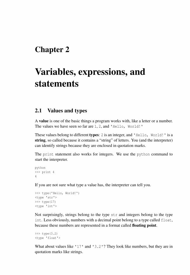
2.1 Values and types

A value is one of the basic things a program works with, like a letter or a number.

The values we have seen so far are 1, 2, and 'Hello, World!'

These values belong to different types: 2 is an integer, and 'Hello, World!' is a

string, so called because it contains a “string” of letters. You (and the interpreter)

can identify strings because they are enclosed in quotation marks.

The print statement also works for integers. We use the python command to

start the interpreter.

python

>>> print 4

4

If you are not sure what type a value has, the interpreter can tell you.

>>> type('Hello, World!')

<type 'str'>

>>> type(17)

<type 'int'>

Not surprisingly, strings belong to the type str and integers belong to the type

int. Less obviously, numbers with a decimal point belong to a type called float,

because these numbers are represented in a format called floating point.

>>> type(3.2)

<type 'float'>

What about values like '17' and '3.2'? They look like numbers, but they are in

quotation marks like strings.

20 Chapter 2. Variables, expressions, and statements

>>> type('17')

<type 'str'>

>>> type('3.2')

<type 'str'>

They’re strings.

When you type a large integer, you might be tempted to use commas between

groups of three digits, as in 1,000,000. This is not a legal integer in Python, but

it is legal:

>>> print 1,000,000

1 0 0

Well, that’s not what we expected at all! Python interprets 1,000,000 as a comma-

separated sequence of integers, which it prints with spaces between.

This is the first example we have seen of a semantic error: the code runs without

producing an error message, but it doesn’t do the “right” thing.

2.2 Variables

One of the most powerful features of a programming language is the ability to

manipulate variables. A variable is a name that refers to a value.

An assignment statement creates new variables and gives them values:

>>> message = 'And now for something completely different'

>>> n = 17

>>> pi = 3.1415926535897931

This example makes three assignments. The first assigns a string to a new vari-

able named message; the second assigns the integer 17 to n; the third assigns the

(approximate) value of π to pi.

To display the value of a variable, you can use a print statement:

>>> print n

17

>>> print pi

3.14159265359

The type of a variable is the type of the value it refers to.

>>> type(message)

<type 'str'>

>>> type(n)

<type 'int'>

>>> type(pi)

<type 'float'>

2.3. Variable names and keywords 21

2.3 Variable names and keywords

Programmers generally choose names for their variables that are meaningful and

document what the variable is used for.

Variable names can be arbitrarily long. They can contain both letters and numbers,

but they cannot start with a number. It is legal to use uppercase letters, but it is a

good idea to begin variable names with a lowercase letter (you’ll see why later).

The underscore character (_) can appear in a name. It is often used in names with

multiple words, such as my_name or airspeed_of_unladen_swallow. Variable

names can start with an underscore character, but we generally avoid doing this

unless we are writing library code for others to use.

If you give a variable an illegal name, you get a syntax error:

>>> 76trombones = 'big parade'


>>> more@ = 1000000


>>> class = 'Advanced Theoretical Zymurgy'


76trombones is illegal because it begins with a number. more@ is illegal because

it contains an illegal character, @. But what’s wrong with class?

It turns out that class is one of Python’s keywords. The interpreter uses keywords

to recognize the structure of the program, and they cannot be used as variable

names.

Python reserves 31 keywords1 for its use:

and del from not while

as elif global or with

assert else if pass yield

break except import print

class exec in raise

continue finally is return

def for lambda try

You might want to keep this list handy. If the interpreter complains about one of

your variable names and you don’t know why, see if it is on this list.

2.4 Statements

A statement is a unit of code that the Python interpreter can execute. We have

seen two kinds of statements: print and assignment.

When you type a statement in interactive mode, the interpreter executes it and

displays the result, if there is one.

1In Python 3.0, exec is no longer a keyword, but nonlocal is.


A script usually contains a sequence of statements. If there is more than one

statement, the results appear one at a time as the statements execute.

For example, the script

print 1

x = 2

print x

produces the output

1

2

The assignment statement produces no output.

2.5 Operators and operands

Operators are special symbols that represent computations like addition and mul-

tiplication. The values the operator is applied to are called operands.

The operators +, -, *, /, and ** perform addition, subtraction, multiplication,

division, and exponentiation, as in the following examples:

20+32 hour-1 hour*60+minute minute/60 5**2 (5+9)*(15-7)

The division operator might not do what you expect:

>>> minute = 59

>>> minute/60

0

The value of minute is 59, and in conventional arithmetic 59 divided by 60 is

0.98333, not 0. The reason for the discrepancy is that Python is performing floor

division2.

When both of the operands are integers, the result is also an integer; floor division

chops off the fractional part, so in this example it truncates the answer to zero.

If either of the operands is a floating-point number, Python performs floating-point

division, and the result is a float:

>>> minute/60.0

0.98333333333333328

2In Python 3.0, the result of this division is a float. In Python 3.0, the new operator // performs

integer division.

2.6. Expressions 23

2.6 Expressions

An expression is a combination of values, variables, and operators. A value all

by itself is considered an expression, and so is a variable, so the following are all

legal expressions (assuming that the variable x has been assigned a value):

17

x

x + 17

If you type an expression in interactive mode, the interpreter evaluates it and

displays the result:

>>> 1 + 1

2

But in a script, an expression all by itself doesn’t do anything! This is a common

source of confusion for beginners.

Exercise 2.1 Type the following statements in the Python interpreter to see what

they do:

5

x = 5

x + 1

2.7 Order of operations

When more than one operator appears in an expression, the order of evaluation

depends on the rules of precedence. For mathematical operators, Python follows

mathematical convention. The acronym PEMDAS is a useful way to remember

the rules:

• Parentheses have the highest precedence and can be used to force an expres-

sion to evaluate in the order you want. Since expressions in parentheses are

evaluated first, 2 * (3-1) is 4, and (1+1)**(5-2) is 8. You can also use

parentheses to make an expression easier to read, as in (minute * 100) /

60, even if it doesn’t change the result.

• Exponentiation has the next highest precedence, so 2**1+1 is 3, not 4, and

3*1**3 is 3, not 27.

• Multiplication and Division have the same precedence, which is higher than

Addition and Subtraction, which also have the same precedence. So 2*3-1

is 5, not 4, and 6+4/2 is 8, not 5.

• Operators with the same precedence are evaluated from left to right. So the

expression 5-3-1 is 1, not 3, because the 5-3 happens first and then 1 is

subtracted from 2.


When in doubt, always put parentheses in your expressions to make sure the com-

putations are performed in the order you intend.

2.8 Modulus operator

The modulus operator works on integers and yields the remainder when the first

operand is divided by the second. In Python, the modulus operator is a percent

sign (%). The syntax is the same as for other operators:

>>> quotient = 7 / 3

>>> print quotient

2

>>> remainder = 7 % 3

>>> print remainder

1

So 7 divided by 3 is 2 with 1 left over.

The modulus operator turns out to be surprisingly useful. For example, you can

check whether one number is divisible by another—if x % y is zero, then x is

divisible by y.

You can also extract the right-most digit or digits from a number. For example, x

% 10 yields the right-most digit of x (in base 10). Similarly, x % 100 yields the

last two digits.

2.9 String operations

The + operator works with strings, but it is not addition in the mathematical sense.

Instead it performs concatenation, which means joining the strings by linking

them end to end. For example:

>>> first = 10

>>> second = 15

>>> print first+second

25

>>> first = '100'

>>> second = '150'

>>> print first + second

100150

The output of this program is 100150.

2.10 Asking the user for input

Sometimes we would like to take the value for a variable from the user via their

keyboard. Python provides a built-in function called raw_input that gets input

2.11. Comments 25

from the keyboard3. When this function is called, the program stops and waits for

the user to type something. When the user presses Return or Enter, the program

resumes and raw_input returns what the user typed as a string.

>>> input = raw_input()

Some silly stuff

>>> print input

Some silly stuff

Before getting input from the user, it is a good idea to print a prompt telling the

user what to input. You can pass a string to raw_input to be displayed to the user

before pausing for input:

>>> name = raw_input('What is your name?\n')

What is your name?

Chuck

>>> print name

Chuck

The sequence \n at the end of the prompt represents a newline, which is a special

character that causes a line break. That’s why the user’s input appears below the

prompt.

If you expect the user to type an integer, you can try to convert the return value to

int using the int() function:

>>> prompt = 'What...is the airspeed velocity of an unladen swallow?\n'

>>> speed = raw_input(prompt)

What...is the airspeed velocity of an unladen swallow?

17

>>> int(speed)

17

>>> int(speed) + 5

22

But if the user types something other than a string of digits, you get an error:



What do you mean, an African or a European swallow?

>>> int(speed)

ValueError: invalid literal for int()

We will see how to handle this kind of error later.

2.11 Comments

As programs get bigger and more complicated, they get more difficult to read.

Formal languages are dense, and it is often difficult to look at a piece of code and

figure out what it is doing, or why.

3In Python 3.0, this function is named input.


For this reason, it is a good idea to add notes to your programs to explain in

natural language what the program is doing. These notes are called comments,

and in Python they start with the # symbol:

# compute the percentage of the hour that has elapsed

percentage = (minute * 100) / 60

In this case, the comment appears on a line by itself. You can also put comments

at the end of a line:

percentage = (minute * 100) / 60 # percentage of an hour

Everything from the # to the end of the line is ignored—it has no effect on the

program.

Comments are most useful when they document non-obvious features of the code.

It is reasonable to assume that the reader can figure out what the code does; it is

much more useful to explain why.

This comment is redundant with the code and useless:

v = 5 # assign 5 to v

This comment contains useful information that is not in the code:

v = 5 # velocity in meters/second.

Good variable names can reduce the need for comments, but long names can make

complex expressions hard to read, so there is a trade-off.

2.12 Choosing mnemonic variable names

As long as you follow the simple rules of variable naming, and avoid reserved

words, you have a lot of choice when you name your variables. In the beginning,

this choice can be confusing both when you read a program and when you write

your own programs. For example, the following three programs are identical in

terms of what they accomplish, but very different when you read them and try to

understand them.

a = 35.0

b = 12.50

c = a * b

print c

hours = 35.0

rate = 12.50

pay = hours * rate

print pay

x1q3z9ahd = 35.0

x1q3z9afd = 12.50

x1q3p9afd = x1q3z9ahd * x1q3z9afd

print x1q3p9afd

2.12. Choosing mnemonic variable names 27

The Python interpreter sees all three of these programs as exactly the same but

humans see and understand these programs quite differently. Humans will most

quickly understand the intent of the second program because the programmer has

chosen variable names that reflect their intent regarding what data will be stored

in each variable.

We call these wisely chosen variable names “mnemonic variable names”. The

word mnemonic4 means “memory aid”. We choose mnemonic variable names to

help us remember why we created the variable in the first place.

While this all sounds great, and it is a very good idea to use mnemonic variable

names, mnemonic variable names can get in the way of a beginning programmer’s

ability to parse and understand code. This is because beginning programmers have

not yet memorized the reserved words (there are only 31 of them) and sometimes

variables with names that are too descriptive start to look like part of the language

and not just well-chosen variable names.

Take a quick look at the following Python sample code which loops through some

data. We will cover loops soon, but for now try to just puzzle through what this

means:

for word in words:

print word

What is happening here? Which of the tokens (for, word, in, etc.) are reserved

words and which are just variable names? Does Python understand at a funda-

mental level the notion of words? Beginning programmers have trouble separating

what parts of the code must be the same as this example and what parts of the code

are simply choices made by the programmer.

The following code is equivalent to the above code:

for slice in pizza:

print slice

It is easier for the beginning programmer to look at this code and know which

parts are reserved words defined by Python and which parts are simply variable

names chosen by the programmer. It is pretty clear that Python has no fundamental

understanding of pizza and slices and the fact that a pizza consists of a set of one

or more slices.

But if our program is truly about reading data and looking for words in the data,

pizza and slice are very un-mnemonic variable names. Choosing them as vari-

able names distracts from the meaning of the program.

After a pretty short period of time, you will know the most common reserved

words and you will start to see the reserved words jumping out at you:

4See http://en.wikipedia.org/wiki/Mnemonic for an extended description of the word

“mnemonic”.


for word in words:

print word

The parts of the code that are defined by Python (for, in, print, and :) are in bold

and the programmer-chosen variables (word and words) are not in bold. Many text

editors are aware of Python syntax and will color reserved words differently to give

you clues to keep your variables and reserved words separate. After a while you

will begin to read Python and quickly determine what is a variable and what is a

reserved word.

2.13 Debugging

At this point, the syntax error you are most likely to make is an illegal variable

name, like class and yield, which are keywords, or odd˜job and US$, which

contain illegal characters.

If you put a space in a variable name, Python thinks it is two operands without an

operator:

>>> bad name = 5


For syntax errors, the error messages don’t help much. The most common

messages are SyntaxError: invalid syntax and SyntaxError: invalid

token, neither of which is very informative.

The runtime error you are most likely to make is a “use before def;” that is, trying

to use a variable before you have assigned a value. This can happen if you spell a

variable name wrong:

>>> principal = 327.68

>>> interest = principle * rate

NameError: name 'principle' is not defined

Variables names are case sensitive, so LaTeX is not the same as latex.

At this point, the most likely cause of a semantic error is the order of operations.

For example, to evaluate 12π

, you might be tempted to write

>>> 1.0 / 2.0 * pi

But the division happens first, so you would get π/2, which is not the same thing!

There is no way for Python to know what you meant to write, so in this case you

don’t get an error message; you just get the wrong answer.

2.14 Glossary

assignment: A statement that assigns a value to a variable.

2.14. Glossary 29

concatenate: To join two operands end to end.

comment: Information in a program that is meant for other programmers (or any-

one reading the source code) and has no effect on the execution of the pro-

gram.

evaluate: To simplify an expression by performing the operations in order to yield

a single value.

expression: A combination of variables, operators, and values that represents a

single result value.

floating point: A type that represents numbers with fractional parts.

floor division: The operation that divides two numbers and chops off the frac-

tional part.

integer: A type that represents whole numbers.

keyword: A reserved word that is used by the compiler to parse a program; you

cannot use keywords like if, def, and while as variable names.

mnemonic: A memory aid. We often give variables mnemonic names to help us

remember what is stored in the variable.

modulus operator: An operator, denoted with a percent sign (%), that works on

integers and yields the remainder when one number is divided by another.

operand: One of the values on which an operator operates.

operator: A special symbol that represents a simple computation like addition,

multiplication, or string concatenation.

rules of precedence: The set of rules governing the order in which expressions

involving multiple operators and operands are evaluated.

statement: A section of code that represents a command or action. So far, the

statements we have seen are assignments and print statements.

string: A type that represents sequences of characters.

type: A category of values. The types we have seen so far are integers (type int),

floating-point numbers (type float), and strings (type str).

value: One of the basic units of data, like a number or string, that a program

manipulates.

variable: A name that refers to a value.


2.15 Exercises

Exercise 2.2 Write a program that uses raw_input to prompt a user for their

name and then welcomes them.

Enter your name: Chuck

Hello Chuck

Exercise 2.3 Write a program to prompt the user for hours and rate per hour to

compute gross pay.

Enter Hours: 35

Enter Rate: 2.75

Pay: 96.25

We won’t worry about making sure our pay has exactly two digits after the decimal

place for now. If you want, you can play with the built-in Python round function

to properly round the resulting pay to two decimal places.

Exercise 2.4 Assume that we execute the following assignment statements:

width = 17

height = 12.0

For each of the following expressions, write the value of the expression and the

type (of the value of the expression).

1. width/2

2. width/2.0

3. height/3

4. 1 + 2 * 5

Use the Python interpreter to check your answers.

Exercise 2.5 Write a program which prompts the user for a Celsius temperature,

convert the temperature to Fahrenheit, and print out the converted temperature.

Chapter 3

Conditional execution

3.1 Boolean expressions

A boolean expression is an expression that is either true or false. The following

examples use the operator ==, which compares two operands and produces True

if they are equal and False otherwise:

>>> 5 == 5

True

>>> 5 == 6

False

True and False are special values that belong to the type bool; they are not

strings:

>>> type(True)

<type 'bool'>

>>> type(False)

<type 'bool'>

The == operator is one of the comparison operators; the others are:

x != y # x is not equal to y

x > y # x is greater than y

x < y # x is less than y

x >= y # x is greater than or equal to y

x <= y # x is less than or equal to y

x is y # x is the same as y

x is not y # x is not the same as y

Although these operations are probably familiar to you, the Python symbols are

different from the mathematical symbols for the same operations. A common error

is to use a single equal sign (=) instead of a double equal sign (==). Remember

that = is an assignment operator and == is a comparison operator. There is no such

thing as =< or =>.

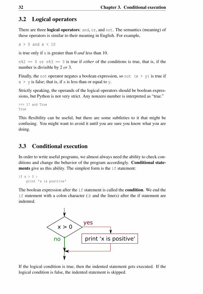
32 Chapter 3. Conditional execution

3.2 Logical operators

There are three logical operators: and, or, and not. The semantics (meaning) of

these operators is similar to their meaning in English. For example,

x > 0 and x < 10

is true only if x is greater than 0 and less than 10.

n%2 == 0 or n%3 == 0 is true if either of the conditions is true, that is, if the

number is divisible by 2 or 3.

Finally, the not operator negates a boolean expression, so not (x > y) is true if

x > y is false; that is, if x is less than or equal to y.

Strictly speaking, the operands of the logical operators should be boolean expres-

sions, but Python is not very strict. Any nonzero number is interpreted as “true.”

>>> 17 and True

True

This flexibility can be useful, but there are some subtleties to it that might be

confusing. You might want to avoid it until you are sure you know what you are

doing.

3.3 Conditional execution

In order to write useful programs, we almost always need the ability to check con-

ditions and change the behavior of the program accordingly. Conditional state-

ments give us this ability. The simplest form is the if statement:

if x > 0 :

print 'x is positive'

The boolean expression after the if statement is called the condition. We end the

if statement with a colon character (:) and the line(s) after the if statement are

indented.

x > 0

print 'x is positive'

yes

no

If the logical condition is true, then the indented statement gets executed. If the

logical condition is false, the indented statement is skipped.

3.4. Alternative execution 33

if statements have the same structure as function definitions or for loops1.The

statement consists of a header line that ends with the colon character (:) followed

by an indented block. Statements like this are called compound statements be-

cause they stretch across more than one line.

There is no limit on the number of statements that can appear in the body, but there

must be at least one. Occasionally, it is useful to have a body with no statements

(usually as a placekeeper for code you haven’t written yet). In that case, you can

use the pass statement, which does nothing.

if x < 0 :

pass # need to handle negative values!

If you enter an if statement in the Python interpreter, the prompt will change

from three chevrons to three dots to indicate you are in the middle of a block of

statements, as shown below:

>>> x = 3

>>> if x < 10:

... print 'Small'

...

Small

>>>

3.4 Alternative execution

A second form of the if statement is alternative execution, in which there are two

possibilities and the condition determines which one gets executed. The syntax

looks like this:

if x%2 == 0 :

print 'x is even'

else :

print 'x is odd'

If the remainder when x is divided by 2 is 0, then we know that x is even, and the

program displays a message to that effect. If the condition is false, the second set

of statements is executed.

x%2 == 0

print 'x is even'

yesno

print 'x is odd'

1We will learn about functions in Chapter 4 and loops in Chapter 5.


Since the condition must either be true or false, exactly one of the alternatives will

be executed. The alternatives are called branches, because they are branches in

the flow of execution.

3.5 Chained conditionals

Sometimes there are more than two possibilities and we need more than two

branches. One way to express a computation like that is a chained conditional:

if x < y:

print 'x is less than y'

elif x > y:

print 'x is greater than y'

else:

print 'x and y are equal'

elif is an abbreviation of “else if.” Again, exactly one branch will be executed.

x < y print 'less'yes

yesx > y

print 'equal'

print 'greater'

There is no limit on the number of elif statements. If there is an else clause, it

has to be at the end, but there doesn’t have to be one.

if choice == 'a':

print 'Bad guess'

elif choice == 'b':

print 'Good guess'

elif choice == 'c':

print 'Close, but not correct'

Each condition is checked in order. If the first is false, the next is checked, and so

on. If one of them is true, the corresponding branch executes, and the statement

ends. Even if more than one condition is true, only the first true branch executes.

3.6. Nested conditionals 35

3.6 Nested conditionals

One conditional can also be nested within another. We could have written the

three-branch example like this:

if x == y:

print 'x and y are equal'

else:

if x < y:

print 'x is less than y'

else:

print 'x is greater than y'

The outer conditional contains two branches. The first branch contains a sim-

ple statement. The second branch contains another if statement, which has two

branches of its own. Those two branches are both simple statements, although

they could have been conditional statements as well.

x == y

print 'greater'

yes

print 'less'

x < y

print 'equal'

no

noyes

Although the indentation of the statements makes the structure apparent, nested

conditionals become difficult to read very quickly. In general, it is a good idea to

avoid them when you can.

Logical operators often provide a way to simplify nested conditional statements.

For example, we can rewrite the following code using a single conditional:

if 0 < x:

if x < 10:

print 'x is a positive single-digit number.'

The print statement is executed only if we make it past both conditionals, so we

can get the same effect with the and operator:

if 0 < x and x < 10:

print 'x is a positive single-digit number.'


3.7 Catching exceptions using try and except

Earlier we saw a code segment where we used the raw_input and int functions to

read and parse an integer number entered by the user. We also saw how treacherous

doing this could be:



What do you mean, an African or a European swallow?

>>> int(speed)

ValueError: invalid literal for int()

>>>

When we are executing these statements in the Python interpreter, we get a new

prompt from the interpreter, think “oops”, and move on to our next statement.

However if you place this code in a Python script and this error occurs, your script

immediately stops in its tracks with a traceback. It does not execute the following

statement.

Here is a sample program to convert a Fahrenheit temperature to a Celsius tem-

perature:

inp = raw_input('Enter Fahrenheit Temperature:')

fahr = float(inp)

cel = (fahr - 32.0) * 5.0 / 9.0

print cel

If we execute this code and give it invalid input, it simply fails with an unfriendly

error message:

python fahren.py

Enter Fahrenheit Temperature:72

22.2222222222

python fahren.py

Enter Fahrenheit Temperature:fred


File "fahren.py", line 2, in <module>

fahr = float(inp)

ValueError: invalid literal for float(): fred

There is a conditional execution structure built into Python to handle these types of

expected and unexpected errors called “try / except”. The idea of try and except

is that you know that some sequence of instruction(s) may have a problem and

you want to add some statements to be executed if an error occurs. These extra

statements (the except block) are ignored if there is no error.

You can think of the try and except feature in Python as an “insurance policy”

on a sequence of statements.

We can rewrite our temperature converter as follows:

3.8. Short-circuit evaluation of logical expressions 37

inp = raw_input('Enter Fahrenheit Temperature:')

try:

fahr = float(inp)

cel = (fahr - 32.0) * 5.0 / 9.0

print cel

except:

print 'Please enter a number'

Python starts by executing the sequence of statements in the try block. If all goes

well, it skips the except block and proceeds. If an exception occurs in the try

block, Python jumps out of the try block and executes the sequence of statements

in the except block.

python fahren2.py

Enter Fahrenheit Temperature:72

22.2222222222

python fahren2.py

Enter Fahrenheit Temperature:fred

Please enter a number

Handling an exception with a try statement is called catching an exception. In

this example, the except clause prints an error message. In general, catching an

exception gives you a chance to fix the problem, or try again, or at least end the

program gracefully.

3.8 Short-circuit evaluation of logical expressions

When Python is processing a logical expression such as x >= 2 and (x/y) >

2, it evaluates the expression from left to right. Because of the definition of and,

if x is less than 2, the expression x >= 2 is False and so the whole expression is

False regardless of whether (x/y) > 2 evaluates to True or False.

When Python detects that there is nothing to be gained by evaluating the rest of

a logical expression, it stops its evaluation and does not do the computations in

the rest of the logical expression. When the evaluation of a logical expression

stops because the overall value is already known, it is called short-circuiting the

evaluation.

While this may seem like a fine point, the short-circuit behavior leads to a clever

technique called the guardian pattern. Consider the following code sequence in

the Python interpreter:

>>> x = 6

>>> y = 2

>>> x >= 2 and (x/y) > 2

True

>>> x = 1

>>> y = 0

>>> x >= 2 and (x/y) > 2


False

>>> x = 6

>>> y = 0

>>> x >= 2 and (x/y) > 2



ZeroDivisionError: integer division or modulo by zero

>>>

The third calculation failed because Python was evaluating (x/y) and y was zero,

which causes a runtime error. But the second example did not fail because the

first part of the expression x >= 2 evaluated to False so the (x/y) was not ever

executed due to the short-circuit rule and there was no error.

We can construct the logical expression to strategically place a guard evaluation

just before the evaluation that might cause an error as follows:

>>> x = 1

>>> y = 0

>>> x >= 2 and y != 0 and (x/y) > 2

False

>>> x = 6

>>> y = 0

>>> x >= 2 and y != 0 and (x/y) > 2

False

>>> x >= 2 and (x/y) > 2 and y != 0



ZeroDivisionError: integer division or modulo by zero

>>>

In the first logical expression, x >= 2 is False so the evaluation stops at the and.

In the second logical expression, x >= 2 is True but y != 0 is False so we never

reach (x/y).

In the third logical expression, the y != 0 is after the (x/y) calculation so the

expression fails with an error.

In the second expression, we say that y != 0 acts as a guard to insure that we

only execute (x/y) if y is non-zero.

3.9 Debugging

The traceback Python displays when an error occurs contains a lot of information,

but it can be overwhelming. The most useful parts are usually:

• What kind of error it was, and

• Where it occurred.

3.10. Glossary 39

Syntax errors are usually easy to find, but there are a few gotchas. Whitespace er-

rors can be tricky because spaces and tabs are invisible and we are used to ignoring

them.

>>> x = 5

>>> y = 6


y = 6

ˆ


In this example, the problem is that the second line is indented by one space. But

the error message points to y, which is misleading. In general, error messages

indicate where the problem was discovered, but the actual error might be earlier

in the code, sometimes on a previous line.

The same is true of runtime errors. Suppose you are trying to compute a signal-to-

noise ratio in decibels. The formula is SNRdb = 10log10(Psignal/Pnoise). In Python,

you might write something like this:

import math

signal_power = 9

noise_power = 10

ratio = signal_power / noise_power

decibels = 10 * math.log10(ratio)

print decibels

But when you run it, you get an error message2:


File "snr.py", line 5, in ?

decibels = 10 * math.log10(ratio)

OverflowError: math range error

The error message indicates line 5, but there is nothing wrong with that line. To

find the real error, it might be useful to print the value of ratio, which turns

out to be 0. The problem is in line 4, because dividing two integers does floor

division. The solution is to represent signal power and noise power with floating-

point values.

In general, error messages tell you where the problem was discovered, but that is

often not where it was caused.

3.10 Glossary

body: The sequence of statements within a compound statement.

boolean expression: An expression whose value is either True or False.

2In Python 3.0, you no longer get an error message; the division operator performs floating-point

division even with integer operands.


branch: One of the alternative sequences of statements in a conditional state-

ment.

chained conditional: A conditional statement with a series of alternative

branches.

comparison operator: One of the operators that compares its operands: ==, !=,

>, <, >=, and <=.

conditional statement: A statement that controls the flow of execution depend-

ing on some condition.

condition: The boolean expression in a conditional statement that determines

which branch is executed.

compound statement: A statement that consists of a header and a body. The

header ends with a colon (:). The body is indented relative to the header.

guardian pattern: Where we construct a logical expression with additional com-

parisons to take advantage of the short-circuit behavior.

logical operator: One of the operators that combines boolean expressions: and,

or, and not.

nested conditional: A conditional statement that appears in one of the branches

of another conditional statement.

traceback: A list of the functions that are executing, printed when an exception

occurs.

short circuit: When Python is part-way through evaluating a logical expression

and stops the evaluation because Python knows the final value for the ex-

pression without needing to evaluate the rest of the expression.

3.11 Exercises

Exercise 3.1 Rewrite your pay computation to give the employee 1.5 times the

hourly rate for hours worked above 40 hours.

Enter Hours: 45

Enter Rate: 10

Pay: 475.0

Exercise 3.2 Rewrite your pay program using try and except so that your pro-

gram handles non-numeric input gracefully by printing a message and exiting the

program. The following shows two executions of the program:

3.11. Exercises 41

Enter Hours: 20

Enter Rate: nine

Error, please enter numeric input

Enter Hours: forty

Error, please enter numeric input

Exercise 3.3 Write a program to prompt for a score between 0.0 and 1.0. If the

score is out of range, print an error message. If the score is between 0.0 and 1.0,

print a grade using the following table:

Score Grade

>= 0.9 A

>= 0.8 B

>= 0.7 C

>= 0.6 D

< 0.6 F

Enter score: 0.95

A

Enter score: perfect

Bad score

Enter score: 10.0

Bad score

Enter score: 0.75

C

Enter score: 0.5

F

Run the program repeatedly as shown above to test the various different values for

input.

Chapter 4

Functions

4.1 Function calls

In the context of programming, a function is a named sequence of statements that

performs a computation. When you define a function, you specify the name and

the sequence of statements. Later, you can “call” the function by name. We have

already seen one example of a function call:

>>> type(32)

<type 'int'>

The name of the function is type. The expression in parentheses is called the

argument of the function. The argument is a value or variable that we are passing

into the function as input to the function. The result, for the type function, is the

type of the argument.

It is common to say that a function “takes” an argument and “returns” a result.

The result is called the return value.

4.2 Built-in functions

Python provides a number of important built-in functions that we can use without

needing to provide the function definition. The creators of Python wrote a set of

functions to solve common problems and included them in Python for us to use.

The max and min functions give us the largest and smallest values in a list, respec-

tively:

>>> max('Hello world')

'w'

>>> min('Hello world')

' '

>>>

44 Chapter 4. Functions

The max function tells us the “largest character” in the string (which turns out to be

the letter “w”) and the min function shows us the smallest character (which turns

out to be a space).

Another very common built-in function is the len function which tells us how

many items are in its argument. If the argument to len is a string, it returns the

number of characters in the string.

>>> len('Hello world')

11

>>>

These functions are not limited to looking at strings. They can operate on any set

of values, as we will see in later chapters.

You should treat the names of built-in functions as reserved words (i.e., avoid

using “max” as a variable name).

4.3 Type conversion functions

Python also provides built-in functions that convert values from one type to an-

other. The int function takes any value and converts it to an integer, if it can, or

complains otherwise:

>>> int('32')

32

>>> int('Hello')

ValueError: invalid literal for int(): Hello

int can convert floating-point values to integers, but it doesn’t round off; it chops

off the fraction part:

>>> int(3.99999)

3

>>> int(-2.3)

-2

float converts integers and strings to floating-point numbers:

>>> float(32)

32.0

>>> float('3.14159')

3.14159

Finally, str converts its argument to a string:

>>> str(32)

'32'

>>> str(3.14159)

'3.14159'

4.4. Random numbers 45

4.4 Random numbers

Given the same inputs, most computer programs generate the same outputs every

time, so they are said to be deterministic. Determinism is usually a good thing,

since we expect the same calculation to yield the same result. For some applica-

tions, though, we want the computer to be unpredictable. Games are an obvious

example, but there are more.

Making a program truly nondeterministic turns out to be not so easy, but there

are ways to make it at least seem nondeterministic. One of them is to use algo-

rithms that generate pseudorandom numbers. Pseudorandom numbers are not

truly random because they are generated by a deterministic computation, but just

by looking at the numbers it is all but impossible to distinguish them from random.

The random module provides functions that generate pseudorandom numbers

(which I will simply call “random” from here on).

The function random returns a random float between 0.0 and 1.0 (including 0.0

but not 1.0). Each time you call random, you get the next number in a long series.

To see a sample, run this loop:

import random

for i in range(10):

x = random.random()

print x

This program produces the following list of 10 random numbers between 0.0 and

up to but not including 1.0.

0.301927091705

0.513787075867

0.319470430881

0.285145917252

0.839069045123

0.322027080731

0.550722110248

0.366591677812

0.396981483964

0.838116437404

Exercise 4.1 Run the program on your system and see what numbers you get.

Run the program more than once and see what numbers you get.

The random function is only one of many functions that handle random numbers.

The function randint takes the parameters low and high, and returns an integer

between low and high (including both).

>>> random.randint(5, 10)

5

>>> random.randint(5, 10)

9


To choose an element from a sequence at random, you can use choice:

>>> t = [1, 2, 3]

>>> random.choice(t)

2

>>> random.choice(t)

3

The random module also provides functions to generate random values from con-

tinuous distributions including Gaussian, exponential, gamma, and a few more.

4.5 Math functions

Python has a math module that provides most of the familiar mathematical func-

tions. Before we can use the module, we have to import it:

>>> import math

This statement creates a module object named math. If you print the module

object, you get some information about it:

>>> print math

<module 'math' from '/usr/lib/python2.5/lib-dynload/math.so'>

The module object contains the functions and variables defined in the module. To

access one of the functions, you have to specify the name of the module and the

name of the function, separated by a dot (also known as a period). This format is

called dot notation.

>>> ratio = signal_power / noise_power

>>> decibels = 10 * math.log10(ratio)

>>> radians = 0.7

>>> height = math.sin(radians)

The first example computes the logarithm base 10 of the signal-to-noise ratio. The

math module also provides a function called log that computes logarithms base e.

The second example finds the sine of radians. The name of the variable is a hint

that sin and the other trigonometric functions (cos, tan, etc.) take arguments in

radians. To convert from degrees to radians, divide by 360 and multiply by 2π:

>>> degrees = 45

>>> radians = degrees / 360.0 * 2 * math.pi

>>> math.sin(radians)

0.707106781187

The expression math.pi gets the variable pi from the math module. The value of

this variable is an approximation of π, accurate to about 15 digits.

If you know your trigonometry, you can check the previous result by comparing it

to the square root of two divided by two:

4.6. Adding new functions 47

>>> math.sqrt(2) / 2.0

0.707106781187

4.6 Adding new functions

So far, we have only been using the functions that come with Python, but it is also

possible to add new functions. A function definition specifies the name of a new

function and the sequence of statements that execute when the function is called.

Once we define a function, we can reuse the function over and over throughout

our program.

Here is an example:

def print_lyrics():

print "I'm a lumberjack, and I'm okay."

print 'I sleep all night and I work all day.'

def is a keyword that indicates that this is a function definition. The name of

the function is print_lyrics. The rules for function names are the same as

for variable names: letters, numbers and some punctuation marks are legal, but

the first character can’t be a number. You can’t use a keyword as the name of a

function, and you should avoid having a variable and a function with the same

name.

The empty parentheses after the name indicate that this function doesn’t take any

arguments. Later we will build functions that take arguments as their inputs.

The first line of the function definition is called the header; the rest is called

the body. The header has to end with a colon and the body has to be indented.

By convention, the indentation is always four spaces. The body can contain any

number of statements.

The strings in the print statements are enclosed in quotes. Single quotes and double

quotes do the same thing; most people use single quotes except in cases like this

where a single quote (which is also an apostrophe) appears in the string.

If you type a function definition in interactive mode, the interpreter prints ellipses

(...) to let you know that the definition isn’t complete:

>>> def print_lyrics():

... print "I'm a lumberjack, and I'm okay."

... print 'I sleep all night and I work all day.'

...

To end the function, you have to enter an empty line (this is not necessary in a

script).

Defining a function creates a variable with the same name.


>>> print print_lyrics

<function print_lyrics at 0xb7e99e9c>

>>> print type(print_lyrics)

<type 'function'>

The value of print_lyrics is a function object, which has type 'function'.

The syntax for calling the new function is the same as for built-in functions:

>>> print_lyrics()

I'm a lumberjack, and I'm okay.

I sleep all night and I work all day.

Once you have defined a function, you can use it inside another function.

For example, to repeat the previous refrain, we could write a function called

repeat_lyrics:

def repeat_lyrics():

print_lyrics()

print_lyrics()

And then call repeat_lyrics:

>>> repeat_lyrics()





But that’s not really how the song goes.

4.7 Definitions and uses

Pulling together the code fragments from the previous section, the whole program

looks like this:

def print_lyrics():

print "I'm a lumberjack, and I'm okay."

print 'I sleep all night and I work all day.'

def repeat_lyrics():

print_lyrics()

print_lyrics()

repeat_lyrics()

This program contains two function definitions: print_lyrics and

repeat_lyrics. Function definitions get executed just like other statements, but

the effect is to create function objects. The statements inside the function do not

get executed until the function is called, and the function definition generates no

output.

4.8. Flow of execution 49

As you might expect, you have to create a function before you can execute it. In

other words, the function definition has to be executed before the first time it is

called.

Exercise 4.2 Move the last line of this program to the top, so the function call

appears before the definitions. Run the program and see what error message you

get.

Exercise 4.3 Move the function call back to the bottom and move the definition of

print_lyrics after the definition of repeat_lyrics. What happens when you

run this program?

4.8 Flow of execution

In order to ensure that a function is defined before its first use, you have to know

the order in which statements are executed, which is called the flow of execution.

Execution always begins at the first statement of the program. Statements are

executed one at a time, in order from top to bottom.

Function definitions do not alter the flow of execution of the program, but remem-

ber that statements inside the function are not executed until the function is called.

A function call is like a detour in the flow of execution. Instead of going to the next

statement, the flow jumps to the body of the function, executes all the statements

there, and then comes back to pick up where it left off.

That sounds simple enough, until you remember that one function can call another.

While in the middle of one function, the program might have to execute the state-

ments in another function. But while executing that new function, the program

might have to execute yet another function!

Fortunately, Python is good at keeping track of where it is, so each time a function

completes, the program picks up where it left off in the function that called it.

When it gets to the end of the program, it terminates.

What’s the moral of this sordid tale? When you read a program, you don’t always

want to read from top to bottom. Sometimes it makes more sense if you follow

the flow of execution.

4.9 Parameters and arguments

Some of the built-in functions we have seen require arguments. For example,

when you call math.sin you pass a number as an argument. Some functions take

more than one argument: math.pow takes two, the base and the exponent.


Inside the function, the arguments are assigned to variables called parameters.

Here is an example of a user-defined function that takes an argument:

def print_twice(bruce):

print bruce

print bruce

This function assigns the argument to a parameter named bruce. When the func-

tion is called, it prints the value of the parameter (whatever it is) twice.

This function works with any value that can be printed.

>>> print_twice('Spam')

Spam

Spam

>>> print_twice(17)

17

17

>>> print_twice(math.pi)

3.14159265359

3.14159265359

The same rules of composition that apply to built-in functions also apply to user-

defined functions, so we can use any kind of expression as an argument for

print_twice:

>>> print_twice('Spam '*4)

Spam Spam Spam Spam

Spam Spam Spam Spam

>>> print_twice(math.cos(math.pi))

-1.0

-1.0

The argument is evaluated before the function is called, so in the examples the

expressions 'Spam '*4 and math.cos(math.pi) are only evaluated once.

You can also use a variable as an argument:

>>> michael = 'Eric, the half a bee.'

>>> print_twice(michael)

Eric, the half a bee.

Eric, the half a bee.

The name of the variable we pass as an argument (michael) has nothing to do

with the name of the parameter (bruce). It doesn’t matter what the value was

called back home (in the caller); here in print_twice, we call everybody bruce.

4.10 Fruitful functions and void functions

Some of the functions we are using, such as the math functions, yield results;

for lack of a better name, I call them fruitful functions. Other functions, like

4.10. Fruitful functions and void functions 51

print_twice, perform an action but don’t return a value. They are called void

functions.

When you call a fruitful function, you almost always want to do something with

the result; for example, you might assign it to a variable or use it as part of an

expression:

x = math.cos(radians)

golden = (math.sqrt(5) + 1) / 2

When you call a function in interactive mode, Python displays the result:

>>> math.sqrt(5)

2.2360679774997898

But in a script, if you call a fruitful function and do not store the result of the

function in a variable, the return value vanishes into the mist!

math.sqrt(5)

This script computes the square root of 5, but since it doesn’t store the result in a

variable or display the result, it is not very useful.

Void functions might display something on the screen or have some other effect,

but they don’t have a return value. If you try to assign the result to a variable, you

get a special value called None.

>>> result = print_twice('Bing')

Bing

Bing

>>> print result

None

The value None is not the same as the string 'None'. It is a special value that has

its own type:

>>> print type(None)

<type 'NoneType'>

To return a result from a function, we use the return statement in our function.

For example, we could make a very simple function called addtwo that adds two

numbers together and returns a result.

def addtwo(a, b):

added = a + b

return added

x = addtwo(3, 5)

print x

When this script executes, the print statement will print out “8” because the

addtwo function was called with 3 and 5 as arguments. Within the function, the

parameters a and b were 3 and 5 respectively. The function computed the sum of


the two numbers and placed it in the local function variable named added. Then

it used the return statement to send the computed value back to the calling code

as the function result, which was assigned to the variable x and printed out.

4.11 Why functions?

It may not be clear why it is worth the trouble to divide a program into functions.

There are several reasons:

• Creating a new function gives you an opportunity to name a group of state-

ments, which makes your program easier to read, understand, and debug.

• Functions can make a program smaller by eliminating repetitive code. Later,

if you make a change, you only have to make it in one place.

• Dividing a long program into functions allows you to debug the parts one at

a time and then assemble them into a working whole.

• Well-designed functions are often useful for many programs. Once you

write and debug one, you can reuse it.

Throughout the rest of the book, often we will use a function definition to explain

a concept. Part of the skill of creating and using functions is to have a function

properly capture an idea such as “find the smallest value in a list of values”. Later

we will show you code that finds the smallest in a list of values and we will present

it to you as a function named min which takes a list of values as its argument and

returns the smallest value in the list.

4.12 Debugging

If you are using a text editor to write your scripts, you might run into problems

with spaces and tabs. The best way to avoid these problems is to use spaces

exclusively (no tabs). Most text editors that know about Python do this by default,

but some don’t.

Tabs and spaces are usually invisible, which makes them hard to debug, so try to

find an editor that manages indentation for you.

Also, don’t forget to save your program before you run it. Some development

environments do this automatically, but some don’t. In that case, the program you

are looking at in the text editor is not the same as the program you are running.

Debugging can take a long time if you keep running the same incorrect program

over and over!

Make sure that the code you are looking at is the code you are running. If you’re

not sure, put something like print 'hello' at the beginning of the program and

run it again. If you don’t see hello, you’re not running the right program!

4.13. Glossary 53

4.13 Glossary

algorithm: A general process for solving a category of problems.

argument: A value provided to a function when the function is called. This value

is assigned to the corresponding parameter in the function.

body: The sequence of statements inside a function definition.

composition: Using an expression as part of a larger expression, or a statement

as part of a larger statement.

deterministic: Pertaining to a program that does the same thing each time it runs,

given the same inputs.

dot notation: The syntax for calling a function in another module by specifying

the module name followed by a dot (period) and the function name.

flow of execution: The order in which statements are executed during a program

run.

fruitful function: A function that returns a value.

function: A named sequence of statements that performs some useful operation.

Functions may or may not take arguments and may or may not produce a

result.

function call: A statement that executes a function. It consists of the function

name followed by an argument list.

function definition: A statement that creates a new function, specifying its name,

parameters, and the statements it executes.

function object: A value created by a function definition. The name of the func-

tion is a variable that refers to a function object.

header: The first line of a function definition.

import statement: A statement that reads a module file and creates a module

object.

module object: A value created by an import statement that provides access to

the data and code defined in a module.

parameter: A name used inside a function to refer to the value passed as an

argument.

pseudorandom: Pertaining to a sequence of numbers that appear to be random,

but are generated by a deterministic program.

return value: The result of a function. If a function call is used as an expression,

the return value is the value of the expression.

void function: A function that does not return a value.


4.14 Exercises

Exercise 4.4 What is the purpose of the ”def” keyword in Python?

a) It is slang that means ”the following code is really cool”

b) It indicates the start of a function

c) It indicates that the following indented section of code is to be stored for later

d) b and c are both true

e) None of the above

Exercise 4.5 What will the following Python program print out?

def fred():

print "Zap"

def jane():

print "ABC"

jane()

fred()

jane()

a) Zap ABC jane fred jane

b) Zap ABC Zap

c) ABC Zap jane

d) ABC Zap ABC

e) Zap Zap Zap

Exercise 4.6 Rewrite your pay computation with time-and-a-half for overtime

and create a function called computepay which takes two parameters (hours and

rate).

Enter Hours: 45

Enter Rate: 10

Pay: 475.0

Exercise 4.7 Rewrite the grade program from the previous chapter using a func-

tion called computegrade that takes a score as its parameter and returns a grade

as a string.

Score Grade

> 0.9 A

> 0.8 B

> 0.7 C

> 0.6 D

<= 0.6 F

Program Execution:

Enter score: 0.95

4.14. Exercises 55

A

Enter score: perfect

Bad score

Enter score: 10.0

Bad score

Enter score: 0.75

C

Enter score: 0.5

F

Run the program repeatedly to test the various different values for input.

Chapter 5

Iteration

5.1 Updating variables

A common pattern in assignment statements is an assignment statement that up-

dates a variable – where the new value of the variable depends on the old.

x = x+1

This means “get the current value of x, add 1, and then update x with the new

value.”

If you try to update a variable that doesn’t exist, you get an error, because Python

evaluates the right side before it assigns a value to x:

>>> x = x+1

NameError: name 'x' is not defined

Before you can update a variable, you have to initialize it, usually with a simple

assignment:

>>> x = 0

>>> x = x+1

Updating a variable by adding 1 is called an increment; subtracting 1 is called a

decrement.

5.2 The while statement

Computers are often used to automate repetitive tasks. Repeating identical or sim-

ilar tasks without making errors is something that computers do well and people

do poorly. Because iteration is so common, Python provides several language

features to make it easier.

One form of iteration in Python is the while statement. Here is a simple program

that counts down from five and then says “Blastoff!”.

58 Chapter 5. Iteration

n = 5

while n > 0:

print n

n = n-1

print 'Blastoff!'

You can almost read the while statement as if it were English. It means, “While n

is greater than 0, display the value of n and then reduce the value of n by 1. When

you get to 0, exit the while statement and display the word Blastoff!”

More formally, here is the flow of execution for a while statement:

1. Evaluate the condition, yielding True or False.

2. If the condition is false, exit the while statement and continue execution at

the next statement.

3. If the condition is true, execute the body and then go back to step 1.

This type of flow is called a loop because the third step loops back around to the

top. We call each time we execute the body of the loop an iteration. For the above

loop, we would say, “It had five iterations”, which means that the body of the loop

was executed five times.

The body of the loop should change the value of one or more variables so that

eventually the condition becomes false and the loop terminates. We call the vari-

able that changes each time the loop executes and controls when the loop finishes

the iteration variable. If there is no iteration variable, the loop will repeat forever,

resulting in an infinite loop.

5.3 Infinite loops

An endless source of amusement for programmers is the observation that the di-

rections on shampoo, “Lather, rinse, repeat,” are an infinite loop because there is

no iteration variable telling you how many times to execute the loop.

In the case of countdown, we can prove that the loop terminates because we know

that the value of n is finite, and we can see that the value of n gets smaller each

time through the loop, so eventually we have to get to 0. Other times a loop is

obviously infinite because it has no iteration variable at all.

5.4 “Infinite loops” and break

Sometimes you don’t know it’s time to end a loop until you get half way through

the body. In that case you can write an infinite loop on purpose and then use the

break statement to jump out of the loop.

5.5. Finishing iterations with continue 59

This loop is obviously an infinite loop because the logical expression on the while

statement is simply the logical constant True:

n = 10

while True:

print n,

n = n - 1

print 'Done!'

If you make the mistake and run this code, you will learn quickly how to stop

a runaway Python process on your system or find where the power-off button is

on your computer. This program will run forever or until your battery runs out

because the logical expression at the top of the loop is always true by virtue of the

fact that the expression is the constant value True.

While this is a dysfunctional infinite loop, we can still use this pattern to build

useful loops as long as we carefully add code to the body of the loop to explicitly

exit the loop using break when we have reached the exit condition.

For example, suppose you want to take input from the user until they type done.

You could write:

while True:

line = raw_input('> ')

if line == 'done':

break

print line

print 'Done!'

The loop condition is True, which is always true, so the loop runs repeatedly until

it hits the break statement.

Each time through, it prompts the user with an angle bracket. If the user types

done, the break statement exits the loop. Otherwise the program echoes whatever

the user types and goes back to the top of the loop. Here’s a sample run:

> hello there

hello there

> finished

finished

> done

Done!

This way of writing while loops is common because you can check the condition

anywhere in the loop (not just at the top) and you can express the stop condition

affirmatively (“stop when this happens”) rather than negatively (“keep going until

that happens.”).

5.5 Finishing iterations with continue

Sometimes you are in an iteration of a loop and want to finish the current iteration

and immediately jump to the next iteration. In that case you can use the continue


statement to skip to the next iteration without finishing the body of the loop for

the current iteration.

Here is an example of a loop that copies its input until the user types “done”, but

treats lines that start with the hash character as lines not to be printed (kind of like

Python comments).

while True:


if line[0] == '#' :

continue

if line == 'done':

break

print line

print 'Done!'

Here is a sample run of this new program with continue added.

> hello there

hello there

> # don't print this

> print this!

print this!

> done

Done!

All the lines are printed except the one that starts with the hash sign because when

the continue is executed, it ends the current iteration and jumps back to the while

statement to start the next iteration, thus skipping the print statement.

5.6 Definite loops using for

Sometimes we want to loop through a set of things such as a list of words, the lines

in a file, or a list of numbers. When we have a list of things to loop through, we

can construct a definite loop using a for statement. We call the while statement

an indefinite loop because it simply loops until some condition becomes False,

whereas the for loop is looping through a known set of items so it runs through

as many iterations as there are items in the set.

The syntax of a for loop is similar to the while loop in that there is a for state-

ment and a loop body:

friends = ['Joseph', 'Glenn', 'Sally']

for friend in friends:

print 'Happy New Year:', friend

print 'Done!'

In Python terms, the variable friends is a list1 of three strings and the for loop

goes through the list and executes the body once for each of the three strings in

the list resulting in this output:

1We will examine lists in more detail in a later chapter.

5.7. Loop patterns 61

Happy New Year: Joseph

Happy New Year: Glenn

Happy New Year: Sally

Done!

Translating this for loop to English is not as direct as the while, but if you think

of friends as a set, it goes like this: “Run the statements in the body of the for loop

once for each friend in the set named friends.”

Looking at the for loop, for and in are reserved Python keywords, and friend

and friends are variables.

for friend in friends:

print ’Happy New Year’, friend

In particular, friend is the iteration variable for the for loop. The variable

friend changes for each iteration of the loop and controls when the for loop

completes. The iteration variable steps successively through the three strings

stored in the friends variable.

5.7 Loop patterns

Often we use a for or while loop to go through a list of items or the contents of

a file and we are looking for something such as the largest or smallest value of the

data we scan through.

These loops are generally constructed by:

• Initializing one or more variables before the loop starts

• Performing some computation on each item in the loop body, possibly

changing the variables in the body of the loop

• Looking at the resulting variables when the loop completes

We will use a list of numbers to demonstrate the concepts and construction of

these loop patterns.

5.7.1 Counting and summing loops

For example, to count the number of items in a list, we would write the following

for loop:

count = 0

for itervar in [3, 41, 12, 9, 74, 15]:

count = count + 1

print 'Count: ', count


We set the variable count to zero before the loop starts, then we write a for loop

to run through the list of numbers. Our iteration variable is named itervar and

while we do not use itervar in the loop, it does control the loop and cause the

loop body to be executed once for each of the values in the list.

In the body of the loop, we add 1 to the current value of count for each of the

values in the list. While the loop is executing, the value of count is the number of

values we have seen “so far”.

Once the loop completes, the value of count is the total number of items. The

total number “falls in our lap” at the end of the loop. We construct the loop so that

we have what we want when the loop finishes.

Another similar loop that computes the total of a set of numbers is as follows:

total = 0

for itervar in [3, 41, 12, 9, 74, 15]:

total = total + itervar

print 'Total: ', total

In this loop we do use the iteration variable. Instead of simply adding one to the

count as in the previous loop, we add the actual number (3, 41, 12, etc.) to the

running total during each loop iteration. If you think about the variable total, it

contains the “running total of the values so far”. So before the loop starts total

is zero because we have not yet seen any values, during the loop total is the

running total, and at the end of the loop total is the overall total of all the values

in the list.

As the loop executes, total accumulates the sum of the elements; a variable used

this way is sometimes called an accumulator.

Neither the counting loop nor the summing loop are particularly useful in practice

because there are built-in functions len() and sum() that compute the number of

items in a list and the total of the items in the list respectively.

5.7.2 Maximum and minimum loops

To find the largest value in a list or sequence, we construct the following loop:

largest = None

print 'Before:', largest

for itervar in [3, 41, 12, 9, 74, 15]:

if largest is None or itervar > largest :

largest = itervar

print 'Loop:', itervar, largest

print 'Largest:', largest

When the program executes, the output is as follows:

5.7. Loop patterns 63

Before: None

Loop: 3 3

Loop: 41 41

Loop: 12 41

Loop: 9 41

Loop: 74 74

Loop: 15 74

Largest: 74

The variable largest is best thought of as the “largest value we have seen so far”.

Before the loop, we set largest to the constant None. None is a special constant

value which we can store in a variable to mark the variable as “empty”.

Before the loop starts, the largest value we have seen so far is None since we

have not yet seen any values. While the loop is executing, if largest is None

then we take the first value we see as the largest so far. You can see in the first

iteration when the value of itervar is 3, since largest is None, we immediately

set largest to be 3.

After the first iteration, largest is no longer None, so the second part of the com-

pound logical expression that checks itervar > largest triggers only when we

see a value that is larger than the “largest so far”. When we see a new “even larger”

value we take that new value for largest. You can see in the program output that

largest progresses from 3 to 41 to 74.

At the end of the loop, we have scanned all of the values and the variable largest

now does contain the largest value in the list.

To compute the smallest number, the code is very similar with one small change:

smallest = None

print 'Before:', smallest

for itervar in [3, 41, 12, 9, 74, 15]:

if smallest is None or itervar < smallest:

smallest = itervar

print 'Loop:', itervar, smallest

print 'Smallest:', smallest

Again, smallest is the “smallest so far” before, during, and after the loop exe-

cutes. When the loop has completed, smallest contains the minimum value in

the list.

Again as in counting and summing, the built-in functions max() and min() make

writing these exact loops unnecessary.

The following is a simple version of the Python built-in min() function:

def min(values):

smallest = None

for value in values:

if smallest is None or value < smallest:

smallest = value

return smallest


In the function version of the smallest code, we removed all of the print state-

ments so as to be equivalent to the min function which is already built in to Python.

5.8 Debugging

As you start writing bigger programs, you might find yourself spending more time

debugging. More code means more chances to make an error and more places for

bugs to hide.

One way to cut your debugging time is “debugging by bisection.” For example,

if there are 100 lines in your program and you check them one at a time, it would

take 100 steps.

Instead, try to break the problem in half. Look at the middle of the program,

or near it, for an intermediate value you can check. Add a print statement (or

something else that has a verifiable effect) and run the program.

If the mid-point check is incorrect, the problem must be in the first half of the

program. If it is correct, the problem is in the second half.

Every time you perform a check like this, you halve the number of lines you have

to search. After six steps (which is much less than 100), you would be down to

one or two lines of code, at least in theory.

In practice it is not always clear what the “middle of the program” is and not

always possible to check it. It doesn’t make sense to count lines and find the exact

midpoint. Instead, think about places in the program where there might be errors

and places where it is easy to put a check. Then choose a spot where you think the

chances are about the same that the bug is before or after the check.

5.9 Glossary

accumulator: A variable used in a loop to add up or accumulate a result.

counter: A variable used in a loop to count the number of times something hap-

pened. We initialize a counter to zero and then increment the counter each

time we want to “count” something.

decrement: An update that decreases the value of a variable.

initialize: An assignment that gives an initial value to a variable that will be up-

dated.

increment: An update that increases the value of a variable (often by one).

infinite loop: A loop in which the terminating condition is never satisfied or for

which there is no terminating condition.

5.10. Exercises 65

iteration: Repeated execution of a set of statements using either a function that

calls itself or a loop.

5.10 Exercises

Exercise 5.1 Write a program which repeatedly reads numbers until the user en-

ters “done”. Once “done” is entered, print out the total, count, and average of

the numbers. If the user enters anything other than a number, detect their mistake

using try and except and print an error message and skip to the next number.

Enter a number: 4

Enter a number: 5

Enter a number: bad data

Invalid input

Enter a number: 7

Enter a number: done

16 3 5.33333333333

Exercise 5.2 Write another program that prompts for a list of numbers as above

and at the end prints out both the maximum and minimum of the numbers instead

of the average.

Chapter 6

Strings

6.1 A string is a sequence

A string is a sequence of characters. You can access the characters one at a time

with the bracket operator:

>>> fruit = 'banana'

>>> letter = fruit[1]

The second statement extracts the character at index position 1 from the fruit

variable and assigns it to the letter variable.

The expression in brackets is called an index. The index indicates which character

in the sequence you want (hence the name).

But you might not get what you expect:

>>> print letter

a

For most people, the first letter of 'banana' is b, not a. But in Python, the index

is an offset from the beginning of the string, and the offset of the first letter is zero.

>>> letter = fruit[0]

>>> print letter

b

So b is the 0th letter (“zero-eth”) of 'banana', a is the 1th letter (“one-eth”), and

n is the 2th (“two-eth”) letter.

b a n n aa[0] [1] [2] [3] [4] [5]

You can use any expression, including variables and operators, as an index, but the

value of the index has to be an integer. Otherwise you get:

>>> letter = fruit[1.5]

TypeError: string indices must be integers

68 Chapter 6. Strings

6.2 Getting the length of a string using len

len is a built-in function that returns the number of characters in a string:


>>> len(fruit)

6

To get the last letter of a string, you might be tempted to try something like this:

>>> length = len(fruit)

>>> last = fruit[length]

IndexError: string index out of range

The reason for the IndexError is that there is no letter in ’banana’ with the

index 6. Since we started counting at zero, the six letters are numbered 0 to 5. To

get the last character, you have to subtract 1 from length:

>>> last = fruit[length-1]

>>> print last

a

Alternatively, you can use negative indices, which count backward from the end

of the string. The expression fruit[-1] yields the last letter, fruit[-2] yields

the second to last, and so on.

6.3 Traversal through a string with a loop

A lot of computations involve processing a string one character at a time. Often

they start at the beginning, select each character in turn, do something to it, and

continue until the end. This pattern of processing is called a traversal. One way

to write a traversal is with a while loop:

index = 0

while index < len(fruit):

letter = fruit[index]

print letter

index = index + 1

This loop traverses the string and displays each letter on a line by itself. The

loop condition is index < len(fruit), so when index is equal to the length of

the string, the condition is false, and the body of the loop is not executed. The

last character accessed is the one with the index len(fruit)-1, which is the last

character in the string.

Exercise 6.1 Write a while loop that starts at the last character in the string and

works its way backwards to the first character in the string, printing each letter on

a separate line, except backwards.

Another way to write a traversal is with a for loop:

6.4. String slices 69

for char in fruit:

print char

Each time through the loop, the next character in the string is assigned to the

variable char. The loop continues until no characters are left.

6.4 String slices

A segment of a string is called a slice. Selecting a slice is similar to selecting a

character:

>>> s = 'Monty Python'

>>> print s[0:5]

Monty

>>> print s[6:12]

Python

The operator [n:m] returns the part of the string from the “n-eth” character to the

“m-eth” character, including the first but excluding the last.

If you omit the first index (before the colon), the slice starts at the beginning of

the string. If you omit the second index, the slice goes to the end of the string:


>>> fruit[:3]

'ban'

>>> fruit[3:]

'ana'

If the first index is greater than or equal to the second the result is an empty string,

represented by two quotation marks:


>>> fruit[3:3]

''

An empty string contains no characters and has length 0, but other than that, it is

the same as any other string.

Exercise 6.2 Given that fruit is a string, what does fruit[:] mean?

6.5 Strings are immutable

It is tempting to use the [] operator on the left side of an assignment, with the

intention of changing a character in a string. For example:

>>> greeting = 'Hello, world!'

>>> greeting[0] = 'J'

TypeError: object does not support item assignment


The “object” in this case is the string and the “item” is the character you tried to

assign. For now, an object is the same thing as a value, but we will refine that

definition later. An item is one of the values in a sequence.

The reason for the error is that strings are immutable, which means you can’t

change an existing string. The best you can do is create a new string that is a

variation on the original:

>>> greeting = 'Hello, world!'

>>> new_greeting = 'J' + greeting[1:]

>>> print new_greeting

Jello, world!

This example concatenates a new first letter onto a slice of greeting. It has no

effect on the original string.

6.6 Looping and counting

The following program counts the number of times the letter a appears in a string:

word = 'banana'

count = 0

for letter in word:

if letter == 'a':

count = count + 1

print count

This program demonstrates another pattern of computation called a counter. The

variable count is initialized to 0 and then incremented each time an a is found.

When the loop exits, count contains the result—the total number of a’s.

Exercise 6.3 Encapsulate this code in a function named count, and generalize it

so that it accepts the string and the letter as arguments.

6.7 The in operator

The word in is a boolean operator that takes two strings and returns True if the

first appears as a substring in the second:

>>> 'a' in 'banana'

True

>>> 'seed' in 'banana'

False

6.8 String comparison

The comparison operators work on strings. To see if two strings are equal:

6.9. string methods 71

if word == 'banana':

print 'All right, bananas.'

Other comparison operations are useful for putting words in alphabetical order:

if word < 'banana':

print 'Your word,' + word + ', comes before banana.'

elif word > 'banana':

print 'Your word,' + word + ', comes after banana.'

else:

print 'All right, bananas.'

Python does not handle uppercase and lowercase letters the same way that people

do. All the uppercase letters come before all the lowercase letters, so:

Your word, Pineapple, comes before banana.

A common way to address this problem is to convert strings to a standard format,

such as all lowercase, before performing the comparison. Keep that in mind in

case you have to defend yourself against a man armed with a Pineapple.

6.9 string methods

Strings are an example of Python objects. An object contains both data (the actual

string itself) and methods, which are effectively functions that are built into the

object and are available to any instance of the object.

Python has a function called dir which lists the methods available for an object.

The type function shows the type of an object and the dir function shows the

available methods.

>>> stuff = 'Hello world'

>>> type(stuff)

<type 'str'>

>>> dir(stuff)

['capitalize', 'center', 'count', 'decode', 'encode',

'endswith', 'expandtabs', 'find', 'format', 'index',

'isalnum', 'isalpha', 'isdigit', 'islower', 'isspace',

'istitle', 'isupper', 'join', 'ljust', 'lower', 'lstrip',

'partition', 'replace', 'rfind', 'rindex', 'rjust',

'rpartition', 'rsplit', 'rstrip', 'split', 'splitlines',

'startswith', 'strip', 'swapcase', 'title', 'translate',

'upper', 'zfill']

>>> help(str.capitalize)

Help on method_descriptor:

capitalize(...)

S.capitalize() -> string

Return a copy of the string S with only its first character

capitalized.

>>>


While the dir function lists the methods, and you can use help to get some

simple documentation on a method, a better source of documentation for string

methods would be https://docs.python.org/2/library/stdtypes.html#

string-methods.

Calling a method is similar to calling a function—it takes arguments and returns

a value—but the syntax is different. We call a method by appending the method

name to the variable name using the period as a delimiter.

For example, the method upper takes a string and returns a new string with all

uppercase letters:

Instead of the function syntax upper(word), it uses the method syntax

word.upper().

>>> word = 'banana'

>>> new_word = word.upper()

>>> print new_word

BANANA

This form of dot notation specifies the name of the method, upper, and the name

of the string to apply the method to, word. The empty parentheses indicate that

this method takes no argument.

A method call is called an invocation; in this case, we would say that we are

invoking upper on the word.

For example, there is a string method named find that searches for the position of

one string within another:

>>> word = 'banana'

>>> index = word.find('a')

>>> print index

1

In this example, we invoke find on word and pass the letter we are looking for as

a parameter.

The find method can find substrings as well as characters:

>>> word.find('na')

2

It can take as a second argument the index where it should start:

>>> word.find('na', 3)

4

One common task is to remove white space (spaces, tabs, or newlines) from the

beginning and end of a string using the strip method:

>>> line = ' Here we go '

>>> line.strip()

'Here we go'

6.10. Parsing strings 73

Some methods such as startswith return boolean values.

>>> line = 'Please have a nice day'

>>> line.startswith('Please')

True

>>> line.startswith('p')

False

You will note that startswith requires case to match, so sometimes we take a line

and map it all to lowercase before we do any checking using the lower method.

>>> line = 'Please have a nice day'

>>> line.startswith('p')

False

>>> line.lower()

'please have a nice day'

>>> line.lower().startswith('p')

True

In the last example, the method lower is called and then we use startswith to

see if the resulting lowercase string starts with the letter “p”. As long as we are

careful with the order, we can make multiple method calls in a single expression.

Exercise 6.4 There is a string method called count that is similar to the function

in the previous exercise. Read the documentation of this method at https://

docs.python.org/2/library/stdtypes.html#string-methods and write an

invocation that counts the number of times the letter a occurs in 'banana'.

6.10 Parsing strings

Often, we want to look into a string and find a substring. For example if we were

presented a series of lines formatted as follows:

From stephen.marquard@ uct.ac.za Sat Jan 5 09:14:16 2008

and we wanted to pull out only the second half of the address (i.e., uct.ac.za)

from each line, we can do this by using the find method and string slicing.

First, we will find the position of the at-sign in the string. Then we will find the

position of the first space after the at-sign. And then we will use string slicing to

extract the portion of the string which we are looking for.

>>> data = 'From [email protected] Sat Jan 5 09:14:16 2008'

>>> atpos = data.find('@')

>>> print atpos

21

>>> sppos = data.find(' ',atpos)

>>> print sppos

31

>>> host = data[atpos+1:sppos]

>>> print host

uct.ac.za

>>>


We use a version of the find method which allows us to specify a position in

the string where we want find to start looking. When we slice, we extract the

characters from “one beyond the at-sign through up to but not including the space

character”.

The documentation for the find method is available at https://docs.python.

org/2/library/stdtypes.html#string-methods.

6.11 Format operator

The format operator, % allows us to construct strings, replacing parts of the

strings with the data stored in variables. When applied to integers, % is the modulus

operator. But when the first operand is a string, % is the format operator.

The first operand is the format string, which contains one or more format se-

quences that specify how the second operand is formatted. The result is a string.

For example, the format sequence '%d' means that the second operand should be

formatted as an integer (d stands for “decimal”):

>>> camels = 42

>>> '%d' % camels

'42'

The result is the string '42', which is not to be confused with the integer value

42.

A format sequence can appear anywhere in the string, so you can embed a value

in a sentence:

>>> camels = 42

>>> 'I have spotted %d camels.' % camels

'I have spotted 42 camels.'

If there is more than one format sequence in the string, the second argument has

to be a tuple1. Each format sequence is matched with an element of the tuple, in

order.

The following example uses '%d' to format an integer, '%g' to format a floating-

point number (don’t ask why), and '%s' to format a string:

>>> 'In %d years I have spotted %g %s.' % (3, 0.1, 'camels')

'In 3 years I have spotted 0.1 camels.'

The number of elements in the tuple must match the number of format sequences

in the string. The types of the elements also must match the format sequences:

1A tuple is a sequence of comma-separated values inside a pair of brackets. We will cover tuples

in Chapter 10

6.12. Debugging 75

>>> '%d %d %d' % (1, 2)

TypeError: not enough arguments for format string

>>> '%d' % 'dollars'

TypeError: illegal argument type for built-in operation

In the first example, there aren’t enough elements; in the second, the element is

the wrong type.

The format operator is powerful, but it can be difficult to use. You can read

more about it at https://docs.python.org/2/library/stdtypes.html#

string-formatting.

6.12 Debugging

A skill that you should cultivate as you program is always asking yourself, “What

could go wrong here?” or alternatively, “What crazy thing might our user do to

crash our (seemingly) perfect program?”

For example, look at the program which we used to demonstrate the while loop

in the chapter on iteration:

while True:


if line[0] == '#' :

continue

if line == 'done':

break

print line

print 'Done!'

Look what happens when the user enters an empty line of input:

> hello there

hello there

> # don't print this

> print this!

print this!

>


File "copytildone.py", line 3, in <module>

if line[0] == '#' :

The code works fine until it is presented an empty line. Then there is no zero-th

character, so we get a traceback. There are two solutions to this to make line three

“safe” even if the line is empty.

One possibility is to simply use the startswith method which returns False if

the string is empty.

if line.startswith('#') :


Another way is to safely write the if statement using the guardian pattern and

make sure the second logical expression is evaluated only where there is at least

one character in the string.:

if len(line) > 0 and line[0] == '#' :

6.13 Glossary

counter: A variable used to count something, usually initialized to zero and then

incremented.

empty string: A string with no characters and length 0, represented by two quo-

tation marks.

format operator: An operator, %, that takes a format string and a tuple and gen-

erates a string that includes the elements of the tuple formatted as specified

by the format string.

format sequence: A sequence of characters in a format string, like %d, that spec-

ifies how a value should be formatted.

format string: A string, used with the format operator, that contains format se-

quences.

flag: A boolean variable used to indicate whether a condition is true.

invocation: A statement that calls a method.

immutable: The property of a sequence whose items cannot be assigned.

index: An integer value used to select an item in a sequence, such as a character

in a string.

item: One of the values in a sequence.

method: A function that is associated with an object and called using dot nota-

tion.

object: Something a variable can refer to. For now, you can use “object” and

“value” interchangeably.

search: A pattern of traversal that stops when it finds what it is looking for.

sequence: An ordered set; that is, a set of values where each value is identified

by an integer index.

slice: A part of a string specified by a range of indices.

traverse: To iterate through the items in a sequence, performing a similar opera-

tion on each.

6.14. Exercises 77

6.14 Exercises

Exercise 6.5 Take the following Python code that stores a string:‘

str = 'X-DSPAM-Confidence: 0.8475'

Use find and string slicing to extract the portion of the string after the colon

character and then use the float function to convert the extracted string into a

floating point number.

Exercise 6.6 Read the documentation of the string methods at https://docs.

python.org/2/library/stdtypes.html#string-methods. You might want

to experiment with some of them to make sure you understand how they work.

strip and replace are particularly useful.

The documentation uses a syntax that might be confusing. For example, in

find(sub[, start[, end]]), the brackets indicate optional arguments. So sub

is required, but start is optional, and if you include start, then end is optional.

Chapter 7

Files

7.1 Persistence

So far, we have learned how to write programs and communicate our intentions

to the Central Processing Unit using conditional execution, functions, and itera-

tions. We have learned how to create and use data structures in the Main Memory.

The CPU and memory are where our software works and runs. It is where all of

the “thinking” happens.

But if you recall from our hardware architecture discussions, once the power is

turned off, anything stored in either the CPU or main memory is erased. So up to

now, our programs have just been transient fun exercises to learn Python.

Unit


Memory

NetworkInput

Software

OutputDevices

CentralProcessing

In this chapter, we start to work with Secondary Memory (or files). Secondary

memory is not erased even when the power is turned off. Or in the case of a USB

flash drive, the data we write from our programs can be removed from the system

and transported to another system.

80 Chapter 7. Files

We will primarily focus on reading and writing text files such as those we create

in a text editor. Later we will see how to work with database files which are binary

files, specifically designed to be read and written through database software.

7.2 Opening files

When we want to read or write a file (say on your hard drive), we first must open

the file. Opening the file communicates with your operating system, which knows

where the data for each file is stored. When you open a file, you are asking the

operating system to find the file by name and make sure the file exists. In this

example, we open the file mbox.txt, which should be stored in the same folder

that you are in when you start Python. You can download this file from www.

py4inf.com/code/mbox.txt

>>> fhand = open('mbox.txt')

>>> print fhand

<open file 'mbox.txt', mode 'r' at 0x1005088b0>

If the open is successful, the operating system returns us a file handle. The file

handle is not the actual data contained in the file, but instead it is a “handle” that

we can use to read the data. You are given a handle if the requested file exists and

you have the proper permissions to read the file.

H

A

N

D

L

E

Your

Program

mbox.txtopenreadwriteclose

From stephen.m..

Return-Path: <p..

Date: Sat, 5 Jan ..

To: source@coll..

From: stephen...

Subject: [sakai]...

Details: http:/...

...

If the file does not exist, open will fail with a traceback and you will not get a

handle to access the contents of the file:

>>> fhand = open('stuff.txt')



IOError: [Errno 2] No such file or directory: 'stuff.txt'

Later we will use try and except to deal more gracefully with the situation where

we attempt to open a file that does not exist.

7.3. Text files and lines 81

7.3 Text files and lines

A text file can be thought of as a sequence of lines, much like a Python string can

be thought of as a sequence of characters. For example, this is a sample of a text

file which records mail activity from various individuals in an open source project

development team:

From [email protected] Sat Jan 5 09:14:16 2008

Return-Path: <[email protected]>

Date: Sat, 5 Jan 2008 09:12:18 -0500

To: [email protected]

From: [email protected]

Subject: [sakai] svn commit: r39772 - content/branches/

Details: http://source.sakaiproject.org/viewsvn/?view=rev&rev=39772

...

The entire file of mail interactions is available from www.py4inf.com/code/

mbox.txt and a shortened version of the file is available from www.py4inf.com/

code/mbox-short.txt. These files are in a standard format for a file containing

multiple mail messages. The lines which start with “From ” separate the mes-

sages and the lines which start with “From:” are part of the messages. For more

information about the mbox format, see en.wikipedia.org/wiki/Mbox.

To break the file into lines, there is a special character that represents the “end of

the line” called the newline character.

In Python, we represent the newline character as a backslash-n in string constants.

Even though this looks like two characters, it is actually a single character. When

we look at the variable by entering “stuff” in the interpreter, it shows us the \n

in the string, but when we use print to show the string, we see the string broken

into two lines by the newline character.

>>> stuff = 'Hello\nWorld!'

>>> stuff

'Hello\nWorld!'

>>> print stuff

Hello

World!

>>> stuff = 'X\nY'

>>> print stuff

X

Y

>>> len(stuff)

3

You can also see that the length of the string 'X\nY' is three characters because

the newline character is a single character.

So when we look at the lines in a file, we need to imagine that there is a special

invisible character called the newline at the end of each line that marks the end of

the line.

So the newline character separates the characters in the file into lines.

82 Chapter 7. Files

7.4 Reading files

While the file handle does not contain the data for the file, it is quite easy to

construct a for loop to read through and count each of the lines in a file:

fhand = open('mbox.txt')

count = 0

for line in fhand:

count = count + 1

print 'Line Count:', count

python open.py

Line Count: 132045

We can use the file handle as the sequence in our for loop. Our for loop simply

counts the number of lines in the file and prints them out. The rough translation

of the for loop into English is, “for each line in the file represented by the file

handle, add one to the count variable.”

The reason that the open function does not read the entire file is that the file might

be quite large with many gigabytes of data. The open statement takes the same

amount of time regardless of the size of the file. The for loop actually causes the

data to be read from the file.

When the file is read using a for loop in this manner, Python takes care of splitting

the data in the file into separate lines using the newline character. Python reads

each line through the newline and includes the newline as the last character in the

line variable for each iteration of the for loop.

Because the for loop reads the data one line at a time, it can efficiently read and

count the lines in very large files without running out of main memory to store

the data. The above program can count the lines in any size file using very little

memory since each line is read, counted, and then discarded.

If you know the file is relatively small compared to the size of your main memory,

you can read the whole file into one string using the read method on the file

handle.

>>> fhand = open('mbox-short.txt')

>>> inp = fhand.read()

>>> print len(inp)

94626

>>> print inp[:20]

From stephen.marquar

In this example, the entire contents (all 94,626 characters) of the file

mbox-short.txt are read directly into the variable inp. We use string slicing

to print out the first 20 characters of the string data stored in inp.

When the file is read in this manner, all the characters including all of the lines

and newline characters are one big string in the variable inp. Remember that this

7.5. Searching through a file 83

form of the open function should only be used if the file data will fit comfortably

in the main memory of your computer.

If the file is too large to fit in main memory, you should write your program to

read the file in chunks using a for or while loop.

7.5 Searching through a file

When you are searching through data in a file, it is a very common pattern to read

through a file, ignoring most of the lines and only processing lines which meet

a particular condition. We can combine the pattern for reading a file with string

methods to build simple search mechanisms.

For example, if we wanted to read a file and only print out lines which started with

the prefix “From:”, we could use the string method startswith to select only those

lines with the desired prefix:

fhand = open('mbox-short.txt')

for line in fhand:

if line.startswith('From:') :

print line

When this program runs, we get the following output:





...

The output looks great since the only lines we are seeing are those which start with

“From:”, but why are we seeing the extra blank lines? This is due to that invisible

newline character. Each of the lines ends with a newline, so the print statement

prints the string in the variable line which includes a newline and then print adds

another newline, resulting in the double spacing effect we see.

We could use line slicing to print all but the last character, but a simpler approach

is to use the rstrip method which strips whitespace from the right side of a string

as follows:


for line in fhand:

line = line.rstrip()

if line.startswith('From:') :

print line

When this program runs, we get the following output:

84 Chapter 7. Files








...

As your file processing programs get more complicated, you may want to structure

your search loops using continue. The basic idea of the search loop is that you

are looking for “interesting” lines and effectively skipping “uninteresting” lines.

And then when we find an interesting line, we do something with that line.

We can structure the loop to follow the pattern of skipping uninteresting lines as

follows:


for line in fhand:


# Skip 'uninteresting lines'

if not line.startswith('From:') :

continue

# Process our 'interesting' line

print line

The output of the program is the same. In English, the uninteresting lines are

those which do not start with “From:”, which we skip using continue. For the

“interesting” lines (i.e., those that start with “From:”) we perform the processing

on those lines.

We can use the find string method to simulate a text editor search that finds lines

where the search string is anywhere in the line. Since find looks for an occurrence

of a string within another string and either returns the position of the string or -1

if the string was not found, we can write the following loop to show lines which

contain the string “@uct.ac.za” (i.e., they come from the University of Cape Town

in South Africa):


for line in fhand:


if line.find('@uct.ac.za') == -1 :

continue

print line

Which produces the following output:


X-Authentication-Warning: set sender to [email protected] using -f


Author: [email protected]

From [email protected] Fri Jan 4 07:02:32 2008

X-Authentication-Warning: set sender to [email protected] using -f

7.6. Letting the user choose the file name 85



...

7.6 Letting the user choose the file name

We really do not want to have to edit our Python code every time we want to

process a different file. It would be more usable to ask the user to enter the file

name string each time the program runs so they can use our program on different

files without changing the Python code.

This is quite simple to do by reading the file name from the user using raw_input

as follows:

fname = raw_input('Enter the file name: ')

fhand = open(fname)

count = 0

for line in fhand:

if line.startswith('Subject:') :

count = count + 1

print 'There were', count, 'subject lines in', fname

We read the file name from the user and place it in a variable named fname and

open that file. Now we can run the program repeatedly on different files.

python search6.py

Enter the file name: mbox.txt

There were 1797 subject lines in mbox.txt

python search6.py

Enter the file name: mbox-short.txt

There were 27 subject lines in mbox-short.txt

Before peeking at the next section, take a look at the above program and ask

yourself, “What could go possibly wrong here?” or “What might our friendly user

do that would cause our nice little program to ungracefully exit with a traceback,

making us look not-so-cool in the eyes of our users?”

7.7 Using try, except, and open

I told you not to peek. This is your last chance.

What if our user types something that is not a file name?

python search6.py

Enter the file name: missing.txt


File "search6.py", line 2, in <module>

fhand = open(fname)

IOError: [Errno 2] No such file or directory: 'missing.txt'

86 Chapter 7. Files

python search6.py

Enter the file name: na na boo boo



fhand = open(fname)

IOError: [Errno 2] No such file or directory: 'na na boo boo'

Do not laugh, users will eventually do every possible thing they can do to break

your programs—either on purpose or with malicious intent. As a matter of fact,

an important part of any software development team is a person or group called

Quality Assurance (or QA for short) whose very job it is to do the craziest things

possible in an attempt to break the software that the programmer has created.

The QA team is responsible for finding the flaws in programs before we have

delivered the program to the end users who may be purchasing the software or

paying our salary to write the software. So the QA team is the programmer’s best

friend.

So now that we see the flaw in the program, we can elegantly fix it using the

try/except structure. We need to assume that the open call might fail and add

recovery code when the open fails as follows:


try:

fhand = open(fname)

except:

print 'File cannot be opened:', fname

exit()

count = 0

for line in fhand:

if line.startswith('Subject:') :

count = count + 1

print 'There were', count, 'subject lines in', fname

The exit function terminates the program. It is a function that we call that never

returns. Now when our user (or QA team) types in silliness or bad file names, we

“catch” them and recover gracefully:

python search7.py



python search7.py


File cannot be opened: na na boo boo

Protecting the open call is a good example of the proper use of try and except in

a Python program. We use the term “Pythonic” when we are doing something the

“Python way”. We might say that the above example is the Pythonic way to open

a file.

7.8. Writing files 87

Once you become more skilled in Python, you can engage in repartee with other

Python programmers to decide which of two equivalent solutions to a problem

is “more Pythonic”. The goal to be “more Pythonic” captures the notion that

programming is part engineering and part art. We are not always interested in

just making something work, we also want our solution to be elegant and to be

appreciated as elegant by our peers.

7.8 Writing files

To write a file, you have to open it with mode 'w' as a second parameter:

>>> fout = open('output.txt', 'w')

>>> print fout

<open file 'output.txt', mode 'w' at 0xb7eb2410>

If the file already exists, opening it in write mode clears out the old data and starts

fresh, so be careful! If the file doesn’t exist, a new one is created.

The write method of the file handle object puts data into the file.

>>> line1 = "This here's the wattle,\n"

>>> fout.write(line1)

Again, the file object keeps track of where it is, so if you call write again, it adds

the new data to the end.

We must make sure to manage the ends of lines as we write to the file by explicitly

inserting the newline character when we want to end a line. The print statement

automatically appends a newline, but the write method does not add the newline

automatically.

>>> line2 = 'the emblem of our land.\n'

>>> fout.write(line2)

When you are done writing, you have to close the file to make sure that the last bit

of data is physically written to the disk so it will not be lost if the power goes off.

>>> fout.close()

We could close the files which we open for read as well, but we can be a little

sloppy if we are only opening a few files since Python makes sure that all open

files are closed when the program ends. When we are writing files, we want to

explicitly close the files so as to leave nothing to chance.

7.9 Debugging

When you are reading and writing files, you might run into problems with whites-

pace. These errors can be hard to debug because spaces, tabs, and newlines are

normally invisible:

88 Chapter 7. Files

>>> s = '1 2\t 3\n 4'

>>> print s

1 2 3

4

The built-in function repr can help. It takes any object as an argument and re-

turns a string representation of the object. For strings, it represents whitespace

characters with backslash sequences:

>>> print repr(s)

'1 2\t 3\n 4'

This can be helpful for debugging.

One other problem you might run into is that different systems use different char-

acters to indicate the end of a line. Some systems use a newline, represented \n.

Others use a return character, represented \r. Some use both. If you move files

between different systems, these inconsistencies might cause problems.

For most systems, there are applications to convert from one format to another.

You can find them (and read more about this issue) at wikipedia.org/wiki/

Newline. Or, of course, you could write one yourself.

7.10 Glossary

catch: To prevent an exception from terminating a program using the try and

except statements.

newline: A special character used in files and strings to indicate the end of a line.

Pythonic: A technique that works elegantly in Python. “Using try and except is

the Pythonic way to recover from missing files”.

Quality Assurance: A person or team focused on insuring the overall quality of a

software product. QA is often involved in testing a product and identifying

problems before the product is released.

text file: A sequence of characters stored in permanent storage like a hard drive.

7.11 Exercises

Exercise 7.1 Write a program to read through a file and print the contents of the

file (line by line) all in upper case. Executing the program will look as follows:

python shout.py

Enter a file name: mbox-short.txt

FROM [email protected] SAT JAN 5 09:14:16 2008

RETURN-PATH: <[email protected]>

7.11. Exercises 89

RECEIVED: FROM MURDER (MAIL.UMICH.EDU [141.211.14.90])

BY FRANKENSTEIN.MAIL.UMICH.EDU (CYRUS V2.3.8) WITH LMTPA;

SAT, 05 JAN 2008 09:14:16 -0500

You can download the file from www.py4inf.com/code/mbox-short.txt

Exercise 7.2 Write a program to prompt for a file name, and then read through

the file and look for lines of the form:

X-DSPAM-Confidence: 0.8475

When you encounter a line that starts with “X-DSPAM-Confidence:” pull apart

the line to extract the floating-point number on the line. Count these lines and

then compute the total of the spam confidence values from these lines. When you

reach the end of the file, print out the average spam confidence.


Average spam confidence: 0.894128046745

Enter the file name: mbox-short.txt

Average spam confidence: 0.750718518519

Test your file on the mbox.txt and mbox-short.txt files.

Exercise 7.3 Sometimes when programmers get bored or want to have a bit of fun,

they add a harmless Easter Egg to their program (en.wikipedia.org/wiki/

Easter_egg_(media)). Modify the program that prompts the user for the file

name so that it prints a funny message when the user types in the exact file name

“na na boo boo”. The program should behave normally for all other files which

exist and don’t exist. Here is a sample execution of the program:

python egg.py



python egg.py

Enter the file name: missing.tyxt

File cannot be opened: missing.tyxt

python egg.py


NA NA BOO BOO TO YOU - You have been punk'd!

We are not encouraging you to put Easter Eggs in your programs—this is just an

exercise.

90 Chapter 7. Files

Chapter 8

Lists

8.1 A list is a sequence

Like a string, a list is a sequence of values. In a string, the values are characters;

in a list, they can be any type. The values in list are called elements or sometimes

items.

There are several ways to create a new list; the simplest is to enclose the elements

in square brackets ([ and ]):

[10, 20, 30, 40]

['crunchy frog', 'ram bladder', 'lark vomit']

The first example is a list of four integers. The second is a list of three strings.

The elements of a list don’t have to be the same type. The following list contains

a string, a float, an integer, and (lo!) another list:

['spam', 2.0, 5, [10, 20]]

A list within another list is nested.

A list that contains no elements is called an empty list; you can create one with

empty brackets, [].

As you might expect, you can assign list values to variables:

>>> cheeses = ['Cheddar', 'Edam', 'Gouda']

>>> numbers = [17, 123]

>>> empty = []

>>> print cheeses, numbers, empty

['Cheddar', 'Edam', 'Gouda'] [17, 123] []

8.2 Lists are mutable

The syntax for accessing the elements of a list is the same as for accessing the

characters of a string—the bracket operator. The expression inside the brackets

specifies the index. Remember that the indices start at 0:

92 Chapter 8. Lists

>>> print cheeses[0]

Cheddar

Unlike strings, lists are mutable because you can change the order of items in a

list or reassign an item in a list. When the bracket operator appears on the left side

of an assignment, it identifies the element of the list that will be assigned.

>>> numbers = [17, 123]

>>> numbers[1] = 5

>>> print numbers

[17, 5]

The one-eth element of numbers, which used to be 123, is now 5.

You can think of a list as a relationship between indices and elements. This rela-

tionship is called a mapping; each index “maps to” one of the elements.

List indices work the same way as string indices:

• Any integer expression can be used as an index.

• If you try to read or write an element that does not exist, you get an

IndexError.

• If an index has a negative value, it counts backward from the end of the list.

The in operator also works on lists.

>>> cheeses = ['Cheddar', 'Edam', 'Gouda']

>>> 'Edam' in cheeses

True

>>> 'Brie' in cheeses

False

8.3 Traversing a list

The most common way to traverse the elements of a list is with a for loop. The

syntax is the same as for strings:

for cheese in cheeses:

print cheese

This works well if you only need to read the elements of the list. But if you want

to write or update the elements, you need the indices. A common way to do that

is to combine the functions range and len:

for i in range(len(numbers)):

numbers[i] = numbers[i] * 2

8.4. List operations 93

This loop traverses the list and updates each element. len returns the number of

elements in the list. range returns a list of indices from 0 to n−1, where n is the

length of the list. Each time through the loop, i gets the index of the next element.

The assignment statement in the body uses i to read the old value of the element

and to assign the new value.

A for loop over an empty list never executes the body:

for x in empty:

print 'This never happens.'

Although a list can contain another list, the nested list still counts as a single

element. The length of this list is four:

['spam', 1, ['Brie', 'Roquefort', 'Pol le Veq'], [1, 2, 3]]

8.4 List operations

The + operator concatenates lists:

>>> a = [1, 2, 3]

>>> b = [4, 5, 6]

>>> c = a + b

>>> print c

[1, 2, 3, 4, 5, 6]

Similarly, the * operator repeats a list a given number of times:

>>> [0] * 4

[0, 0, 0, 0]

>>> [1, 2, 3] * 3

[1, 2, 3, 1, 2, 3, 1, 2, 3]

The first example repeats [0] four times. The second example repeats the list [1,

2, 3] three times.

8.5 List slices

The slice operator also works on lists:

>>> t = ['a', 'b', 'c', 'd', 'e', 'f']

>>> t[1:3]

['b', 'c']

>>> t[:4]

['a', 'b', 'c', 'd']

>>> t[3:]

['d', 'e', 'f']

If you omit the first index, the slice starts at the beginning. If you omit the second,

the slice goes to the end. So if you omit both, the slice is a copy of the whole list.

94 Chapter 8. Lists

>>> t[:]

['a', 'b', 'c', 'd', 'e', 'f']

Since lists are mutable, it is often useful to make a copy before performing opera-

tions that fold, spindle, or mutilate lists.

A slice operator on the left side of an assignment can update multiple elements:

>>> t = ['a', 'b', 'c', 'd', 'e', 'f']

>>> t[1:3] = ['x', 'y']

>>> print t

['a', 'x', 'y', 'd', 'e', 'f']

8.6 List methods

Python provides methods that operate on lists. For example, append adds a new

element to the end of a list:

>>> t = ['a', 'b', 'c']

>>> t.append('d')

>>> print t

['a', 'b', 'c', 'd']

extend takes a list as an argument and appends all of the elements:

>>> t1 = ['a', 'b', 'c']

>>> t2 = ['d', 'e']

>>> t1.extend(t2)

>>> print t1

['a', 'b', 'c', 'd', 'e']

This example leaves t2 unmodified.

sort arranges the elements of the list from low to high:

>>> t = ['d', 'c', 'e', 'b', 'a']

>>> t.sort()

>>> print t

['a', 'b', 'c', 'd', 'e']

Most list methods are void; they modify the list and return None. If you acciden-

tally write t = t.sort(), you will be disappointed with the result.

8.7 Deleting elements

There are several ways to delete elements from a list. If you know the index of the

element you want, you can use pop:

8.8. Lists and functions 95

>>> t = ['a', 'b', 'c']

>>> x = t.pop(1)

>>> print t

['a', 'c']

>>> print x

b

pop modifies the list and returns the element that was removed. If you don’t

provide an index, it deletes and returns the last element.

If you don’t need the removed value, you can use the del operator:

>>> t = ['a', 'b', 'c']

>>> del t[1]

>>> print t

['a', 'c']

If you know the element you want to remove (but not the index), you can use

remove:

>>> t = ['a', 'b', 'c']

>>> t.remove('b')

>>> print t

['a', 'c']

The return value from remove is None.

To remove more than one element, you can use del with a slice index:

>>> t = ['a', 'b', 'c', 'd', 'e', 'f']

>>> del t[1:5]

>>> print t

['a', 'f']

As usual, the slice selects all the elements up to, but not including, the second

index.

8.8 Lists and functions

There are a number of built-in functions that can be used on lists that allow you to

quickly look through a list without writing your own loops:

>>> nums = [3, 41, 12, 9, 74, 15]

>>> print len(nums)

6

>>> print max(nums)

74

>>> print min(nums)

3

>>> print sum(nums)

154

>>> print sum(nums)/len(nums)

25

96 Chapter 8. Lists

The sum() function only works when the list elements are numbers. The other

functions (max(), len(), etc.) work with lists of strings and other types that can

be comparable.

We could rewrite an earlier program that computed the average of a list of numbers

entered by the user using a list.

First, the program to compute an average without a list:

total = 0

count = 0

while ( True ) :

inp = raw_input('Enter a number: ')

if inp == 'done' : break

value = float(inp)

total = total + value

count = count + 1

average = total / count

print 'Average:', average

In this program, we have count and total variables to keep the number and

running total of the user’s numbers as we repeatedly prompt the user for a number.

We could simply remember each number as the user entered it and use built-in

functions to compute the sum and count at the end.

numlist = list()

while ( True ) :

inp = raw_input('Enter a number: ')

if inp == 'done' : break

value = float(inp)

numlist.append(value)

average = sum(numlist) / len(numlist)

print 'Average:', average

We make an empty list before the loop starts, and then each time we have a number,

we append it to the list. At the end of the program, we simply compute the sum of

the numbers in the list and divide it by the count of the numbers in the list to come

up with the average.

8.9 Lists and strings

A string is a sequence of characters and a list is a sequence of values, but a list

of characters is not the same as a string. To convert from a string to a list of

characters, you can use list:

>>> s = 'spam'

>>> t = list(s)

>>> print t

['s', 'p', 'a', 'm']

8.10. Parsing lines 97

Because list is the name of a built-in function, you should avoid using it as a

variable name. I also avoid the letter l because it looks too much like the number

1. So that’s why I use t.

The list function breaks a string into individual letters. If you want to break a

string into words, you can use the split method:

>>> s = 'pining for the fjords'

>>> t = s.split()

>>> print t

['pining', 'for', 'the', 'fjords']

>>> print t[2]

the

Once you have used split to break the string into a list of words, you can use the

index operator (square bracket) to look at a particular word in the list.

You can call split with an optional argument called a delimiter that specifies

which characters to use as word boundaries. The following example uses a hyphen

as a delimiter:

>>> s = 'spam-spam-spam'

>>> delimiter = '-'

>>> s.split(delimiter)

['spam', 'spam', 'spam']

join is the inverse of split. It takes a list of strings and concatenates the ele-

ments. join is a string method, so you have to invoke it on the delimiter and pass

the list as a parameter:

>>> t = ['pining', 'for', 'the', 'fjords']

>>> delimiter = ' '

>>> delimiter.join(t)

'pining for the fjords'

In this case the delimiter is a space character, so join puts a space between words.

To concatenate strings without spaces, you can use the empty string, '', as a

delimiter.

8.10 Parsing lines

Usually when we are reading a file we want to do something to the lines other than

just printing the whole line. Often we want to find the “interesting lines” and then

parse the line to find some interesting part of the line. What if we wanted to print

out the day of the week from those lines that start with “From ”?


The split method is very effective when faced with this kind of problem. We

can write a small program that looks for lines where the line starts with “From ”,

split those lines, and then print out the third word in the line:

98 Chapter 8. Lists


for line in fhand:


if not line.startswith('From ') : continue

words = line.split()

print words[2]

Here we also use the contracted form of the if statement where we put the

continue on the same line as the if. This contracted form of the if functions

the same as if the continue were on the next line and indented.

The program produces the following output:

Sat

Fri

Fri

Fri

...

Later, we will learn increasingly sophisticated techniques for picking the lines to

work on and how we pull those lines apart to find the exact bit of information we

are looking for.

8.11 Objects and values

If we execute these assignment statements:

a = 'banana'

b = 'banana'

we know that a and b both refer to a string, but we don’t know whether they refer

to the same string. There are two possible states:

a

b’banana’

a

b

’banana’

’banana’

In one case, a and b refer to two different objects that have the same value. In the

second case, they refer to the same object.

To check whether two variables refer to the same object, you can use the is oper-

ator.

>>> a = 'banana'

>>> b = 'banana'

>>> a is b

True

In this example, Python only created one string object, and both a and b refer to it.

But when you create two lists, you get two objects:

8.12. Aliasing 99

>>> a = [1, 2, 3]

>>> b = [1, 2, 3]

>>> a is b

False

In this case we would say that the two lists are equivalent, because they have the

same elements, but not identical, because they are not the same object. If two

objects are identical, they are also equivalent, but if they are equivalent, they are

not necessarily identical.

Until now, we have been using “object” and “value” interchangeably, but it is more

precise to say that an object has a value. If you execute a = [1,2,3], a refers to

a list object whose value is a particular sequence of elements. If another list has

the same elements, we would say it has the same value.

8.12 Aliasing

If a refers to an object and you assign b = a, then both variables refer to the same

object:

>>> a = [1, 2, 3]

>>> b = a

>>> b is a

True

The association of a variable with an object is called a reference. In this example,

there are two references to the same object.

An object with more than one reference has more than one name, so we say that

the object is aliased.

If the aliased object is mutable, changes made with one alias affect the other:

>>> b[0] = 17

>>> print a

[17, 2, 3]

Although this behavior can be useful, it is error-prone. In general, it is safer to

avoid aliasing when you are working with mutable objects.

For immutable objects like strings, aliasing is not as much of a problem. In this

example:

a = 'banana'

b = 'banana'

it almost never makes a difference whether a and b refer to the same string or not.

100 Chapter 8. Lists

8.13 List arguments

When you pass a list to a function, the function gets a reference to the list. If

the function modifies a list parameter, the caller sees the change. For example,

delete_head removes the first element from a list:

def delete_head(t):

del t[0]

Here’s how it is used:

>>> letters = ['a', 'b', 'c']

>>> delete_head(letters)

>>> print letters

['b', 'c']

The parameter t and the variable letters are aliases for the same object.

It is important to distinguish between operations that modify lists and operations

that create new lists. For example, the append method modifies a list, but the +

operator creates a new list:

>>> t1 = [1, 2]

>>> t2 = t1.append(3)

>>> print t1

[1, 2, 3]

>>> print t2

None

>>> t3 = t1 + [3]

>>> print t3

[1, 2, 3]

>>> t2 is t3

False

This difference is important when you write functions that are supposed to modify

lists. For example, this function does not delete the head of a list:

def bad_delete_head(t):

t = t[1:] # WRONG!

The slice operator creates a new list and the assignment makes t refer to it, but

none of that has any effect on the list that was passed as an argument.

An alternative is to write a function that creates and returns a new list. For exam-

ple, tail returns all but the first element of a list:

def tail(t):

return t[1:]

This function leaves the original list unmodified. Here’s how it is used:

>>> letters = ['a', 'b', 'c']

>>> rest = tail(letters)

>>> print rest

['b', 'c']

8.14. Debugging 101

Exercise 8.1 Write a function called chop that takes a list and modifies it, remov-

ing the first and last elements, and returns None.

Then write a function called middle that takes a list and returns a new list that

contains all but the first and last elements.

8.14 Debugging

Careless use of lists (and other mutable objects) can lead to long hours of debug-

ging. Here are some common pitfalls and ways to avoid them:

1. Don’t forget that most list methods modify the argument and return None.

This is the opposite of the string methods, which return a new string and

leave the original alone.

If you are used to writing string code like this:

word = word.strip()

It is tempting to write list code like this:

t = t.sort() # WRONG!

Because sort returns None, the next operation you perform with t is likely

to fail.

Before using list methods and operators, you should read the documen-

tation carefully and then test them in interactive mode. The meth-

ods and operators that lists share with other sequences (like strings)

are documented at https://docs.python.org/2/library/stdtypes.

html#string-methods. The methods and operators that only apply

to mutable sequences are documented at https://docs.python.org/2/

library/stdtypes.html#mutable-sequence-types.

2. Pick an idiom and stick with it.

Part of the problem with lists is that there are too many ways to do things.

For example, to remove an element from a list, you can use pop, remove,

del, or even a slice assignment.

To add an element, you can use the append method or the + operator. But

don’t forget that these are right:

t.append(x)

t = t + [x]

And these are wrong:

t.append([x]) # WRONG!

t = t.append(x) # WRONG!

t + [x] # WRONG!

t = t + x # WRONG!


Try out each of these examples in interactive mode to make sure you under-

stand what they do. Notice that only the last one causes a runtime error; the

other three are legal, but they do the wrong thing.

3. Make copies to avoid aliasing.

If you want to use a method like sort that modifies the argument, but you

need to keep the original list as well, you can make a copy.

orig = t[:]

t.sort()

In this example you could also use the built-in function sorted, which re-

turns a new, sorted list and leaves the original alone. But in that case you

should avoid using sorted as a variable name!

4. Lists, split, and files

When we read and parse files, there are many opportunities to encounter

input that can crash our program so it is a good idea to revisit the guardian

pattern when it comes writing programs that read through a file and look for

a “needle in the haystack”.

Let’s revisit our program that is looking for the day of the week on the from

lines of our file:


Since we are breaking this line into words, we could dispense with the use

of startswith and simply look at the first word of the line to determine if

we are interested in the line at all. We can use continue to skip lines that

don’t have “From” as the first word as follows:


for line in fhand:


if words[0] != 'From' : continue

print words[2]

This looks much simpler and we don’t even need to do the rstrip to remove

the newline at the end of the file. But is it better?

python search8.py

Sat




IndexError: list index out of range

It kind of works and we see the day from the first line (Sat), but then the

program fails with a traceback error. What went wrong? What messed-up

data caused our elegant, clever, and very Pythonic program to fail?

8.14. Debugging 103

You could stare at it for a long time and puzzle through it or ask someone

for help, but the quicker and smarter approach is to add a print statement.

The best place to add the print statement is right before the line where the

program failed and print out the data that seems to be causing the failure.

Now this approach may generate a lot of lines of output, but at least you will

immediately have some clue as to the problem at hand. So we add a print of

the variable words right before line five. We even add a prefix “Debug:” to

the line so we can keep our regular output separate from our debug output.

for line in fhand:


print 'Debug:', words


print words[2]

When we run the program, a lot of output scrolls off the screen but at the

end, we see our debug output and the traceback so we know what happened

just before the traceback.

Debug: ['X-DSPAM-Confidence:', '0.8475']

Debug: ['X-DSPAM-Probability:', '0.0000']

Debug: []




IndexError: list index out of range

Each debug line is printing the list of words which we get when we split

the line into words. When the program fails, the list of words is empty [].

If we open the file in a text editor and look at the file, at that point it looks

as follows:

X-DSPAM-Result: Innocent

X-DSPAM-Processed: Sat Jan 5 09:14:16 2008


X-DSPAM-Probability: 0.0000


The error occurs when our program encounters a blank line! Of course there

are “zero words” on a blank line. Why didn’t we think of that when we were

writing the code? When the code looks for the first word (word[0]) to check

to see if it matches “From”, we get an “index out of range” error.

This of course is the perfect place to add some guardian code to avoid

checking the first word if the first word is not there. There are many ways

to protect this code; we will choose to check the number of words we have

before we look at the first word:



count = 0

for line in fhand:


# print 'Debug:', words

if len(words) == 0 : continue


print words[2]

First we commented out the debug print statement instead of removing it,

in case our modification fails and we need to debug again. Then we added

a guardian statement that checks to see if we have zero words, and if so, we

use continue to skip to the next line in the file.

We can think of the two continue statements as helping us refine the set of

lines which are “interesting” to us and which we want to process some more.

A line which has no words is “uninteresting” to us so we skip to the next

line. A line which does not have “From” as its first word is uninteresting to

us so we skip it.

The program as modified runs successfully, so perhaps it is correct. Our

guardian statement does make sure that the words[0] will never fail, but

perhaps it is not enough. When we are programming, we must always be

thinking, “What might go wrong?”

Exercise 8.2 Figure out which line of the above program is still not properly

guarded. See if you can construct a text file which causes the program to

fail and then modify the program so that the line is properly guarded and

test it to make sure it handles your new text file.

Exercise 8.3 Rewrite the guardian code in the above example without two

if statements. Instead, use a compound logical expression using the and

logical operator with a single if statement.

8.15 Glossary

aliasing: A circumstance where two or more variables refer to the same object.

delimiter: A character or string used to indicate where a string should be split.

element: One of the values in a list (or other sequence); also called items.

equivalent: Having the same value.

index: An integer value that indicates an element in a list.

identical: Being the same object (which implies equivalence).

list: A sequence of values.

8.16. Exercises 105

list traversal: The sequential accessing of each element in a list.

nested list: A list that is an element of another list.

object: Something a variable can refer to. An object has a type and a value.

reference: The association between a variable and its value.

8.16 Exercises

Exercise 8.4 Download a copy of the file from www.py4inf.com/code/romeo.

txt

Write a program to open the file romeo.txt and read it line by line. For each line,

split the line into a list of words using the split function.

For each word, check to see if the word is already in a list. If the word is not in the

list, add it to the list.

When the program completes, sort and print the resulting words in alphabetical

order.

Enter file: romeo.txt

['Arise', 'But', 'It', 'Juliet', 'Who', 'already',

'and', 'breaks', 'east', 'envious', 'fair', 'grief',

'is', 'kill', 'light', 'moon', 'pale', 'sick', 'soft',

'sun', 'the', 'through', 'what', 'window',

'with', 'yonder']

Exercise 8.5 Write a program to read through the mail box data and when you

find line that starts with “From”, you will split the line into words using the split

function. We are interested in who sent the message, which is the second word on

the From line.


You will parse the From line and print out the second word for each From line,

then you will also count the number of From (not From:) lines and print out a

count at the end.

This is a good sample output with a few lines removed:

python fromcount.py


[email protected]

[email protected]

[email protected]

[...some output removed...]

[email protected]


[email protected]

[email protected]

[email protected]

There were 27 lines in the file with From as the first word

Exercise 8.6 Rewrite the program that prompts the user for a list of numbers and

prints out the maximum and minimum of the numbers at the end when the user

enters “done”. Write the program to store the numbers the user enters in a list

and use the max() and min() functions to compute the maximum and minimum

numbers after the loop completes.

Enter a number: 6

Enter a number: 2

Enter a number: 9

Enter a number: 3

Enter a number: 5

Enter a number: done

Maximum: 9.0

Minimum: 2.0

Chapter 9

Dictionaries

A dictionary is like a list, but more general. In a list, the index positions have to

be integers; in a dictionary, the indices can be (almost) any type.

You can think of a dictionary as a mapping between a set of indices (which are

called keys) and a set of values. Each key maps to a value. The association of a

key and a value is called a key-value pair or sometimes an item.

As an example, we’ll build a dictionary that maps from English to Spanish words,

so the keys and the values are all strings.

The function dict creates a new dictionary with no items. Because dict is the

name of a built-in function, you should avoid using it as a variable name.

>>> eng2sp = dict()

>>> print eng2sp

{}

The curly brackets, {}, represent an empty dictionary. To add items to the dictio-

nary, you can use square brackets:

>>> eng2sp['one'] = 'uno'

This line creates an item that maps from the key ’one’ to the value 'uno'. If we

print the dictionary again, we see a key-value pair with a colon between the key

and value:

>>> print eng2sp

{'one': 'uno'}

This output format is also an input format. For example, you can create a new

dictionary with three items:

>>> eng2sp = {'one': 'uno', 'two': 'dos', 'three': 'tres'}

But if you print eng2sp, you might be surprised:

108 Chapter 9. Dictionaries

>>> print eng2sp

{'one': 'uno', 'three': 'tres', 'two': 'dos'}

The order of the key-value pairs is not the same. In fact, if you type the same

example on your computer, you might get a different result. In general, the order

of items in a dictionary is unpredictable.

But that’s not a problem because the elements of a dictionary are never indexed

with integer indices. Instead, you use the keys to look up the corresponding values:

>>> print eng2sp['two']

'dos'

The key ’two’ always maps to the value 'dos' so the order of the items doesn’t

matter.

If the key isn’t in the dictionary, you get an exception:

>>> print eng2sp['four']

KeyError: 'four'

The len function works on dictionaries; it returns the number of key-value pairs:

>>> len(eng2sp)

3

The in operator works on dictionaries; it tells you whether something appears as

a key in the dictionary (appearing as a value is not good enough).

>>> 'one' in eng2sp

True

>>> 'uno' in eng2sp

False

To see whether something appears as a value in a dictionary, you can use the

method values, which returns the values as a list, and then use the in operator:

>>> vals = eng2sp.values()

>>> 'uno' in vals

True

The in operator uses different algorithms for lists and dictionaries. For lists, it

uses a linear search algorithm. As the list gets longer, the search time gets longer

in direct proportion to the length of the list. For dictionaries, Python uses an

algorithm called a hash table that has a remarkable property—the in operator

takes about the same amount of time no matter how many items there are in a

dictionary. I won’t explain why hash functions are so magical, but you can read

more about it at wikipedia.org/wiki/Hash_table.

Exercise 9.1 Write a program that reads the words in words.txt and stores them

as keys in a dictionary. It doesn’t matter what the values are. Then you can use

the in operator as a fast way to check whether a string is in the dictionary.

9.1. Dictionary as a set of counters 109

9.1 Dictionary as a set of counters

Suppose you are given a string and you want to count how many times each letter

appears. There are several ways you could do it:

1. You could create 26 variables, one for each letter of the alphabet. Then you

could traverse the string and, for each character, increment the correspond-

ing counter, probably using a chained conditional.

2. You could create a list with 26 elements. Then you could convert each

character to a number (using the built-in function ord), use the number as

an index into the list, and increment the appropriate counter.

3. You could create a dictionary with characters as keys and counters as the

corresponding values. The first time you see a character, you would add

an item to the dictionary. After that you would increment the value of an

existing item.

Each of these options performs the same computation, but each of them imple-

ments that computation in a different way.

An implementation is a way of performing a computation; some implementations

are better than others. For example, an advantage of the dictionary implementation

is that we don’t have to know ahead of time which letters appear in the string and

we only have to make room for the letters that do appear.

Here is what the code might look like:

word = 'brontosaurus'

d = dict()

for c in word:

if c not in d:

d[c] = 1

else:

d[c] = d[c] + 1

print d

We are effectively computing a histogram, which is a statistical term for a set of

counters (or frequencies).

The for loop traverses the string. Each time through the loop, if the character c is

not in the dictionary, we create a new item with key c and the initial value 1 (since

we have seen this letter once). If c is already in the dictionary we increment d[c].

Here’s the output of the program:

{'a': 1, 'b': 1, 'o': 2, 'n': 1, 's': 2, 'r': 2, 'u': 2, 't': 1}

The histogram indicates that the letters ’a’ and 'b' appear once; 'o' appears

twice, and so on.


Dictionaries have a method called get that takes a key and a default value. If the

key appears in the dictionary, get returns the corresponding value; otherwise it

returns the default value. For example:

>>> counts = { 'chuck' : 1 , 'annie' : 42, 'jan': 100}

>>> print counts.get('jan', 0)

100

>>> print counts.get('tim', 0)

0

We can use get to write our histogram loop more concisely. Because the get

method automatically handles the case where a key is not in a dictionary, we can

reduce four lines down to one and eliminate the if statement.

word = 'brontosaurus'

d = dict()

for c in word:

d[c] = d.get(c,0) + 1

print d

The use of the get method to simplify this counting loop ends up being a very

commonly used “idiom” in Python and we will use it many times in the rest of the

book. So you should take a moment and compare the loop using the if statement

and in operator with the loop using the get method. They do exactly the same

thing, but one is more succinct.

9.2 Dictionaries and files

One of the common uses of a dictionary is to count the occurrence of words in a

file with some written text. Let’s start with a very simple file of words taken from

the text of Romeo and Juliet.

For the first set of examples, we will use a shortened and simplified version of

the text with no punctuation. Later we will work with the text of the scene with

punctuation included.

But soft what light through yonder window breaks

It is the east and Juliet is the sun

Arise fair sun and kill the envious moon

Who is already sick and pale with grief

We will write a Python program to read through the lines of the file, break each

line into a list of words, and then loop through each of the words in the line and

count each word using a dictionary.

You will see that we have two for loops. The outer loop is reading the lines of

the file and the inner loop is iterating through each of the words on that particular

line. This is an example of a pattern called nested loops because one of the loops

is the outer loop and the other loop is the inner loop.

9.3. Looping and dictionaries 111

Because the inner loop executes all of its iterations each time the outer loop makes

a single iteration, we think of the inner loop as iterating “more quickly” and the

outer loop as iterating more slowly.

The combination of the two nested loops ensures that we will count every word

on every line of the input file.


try:

fhand = open(fname)

except:


exit()

counts = dict()

for line in fhand:


for word in words:

if word not in counts:

counts[word] = 1

else:

counts[word] += 1

print counts

When we run the program, we see a raw dump of all of the counts in unsorted hash

order. (the romeo.txt file is available at www.py4inf.com/code/romeo.txt)

python count1.py

Enter the file name: romeo.txt

{'and': 3, 'envious': 1, 'already': 1, 'fair': 1,

'is': 3, 'through': 1, 'pale': 1, 'yonder': 1,

'what': 1, 'sun': 2, 'Who': 1, 'But': 1, 'moon': 1,

'window': 1, 'sick': 1, 'east': 1, 'breaks': 1,

'grief': 1, 'with': 1, 'light': 1, 'It': 1, 'Arise': 1,

'kill': 1, 'the': 3, 'soft': 1, 'Juliet': 1}

It is a bit inconvenient to look through the dictionary to find the most common

words and their counts, so we need to add some more Python code to get us the

output that will be more helpful.

9.3 Looping and dictionaries

If you use a dictionary as the sequence in a for statement, it traverses the keys of

the dictionary. This loop prints each key and the corresponding value:

counts = { 'chuck' : 1 , 'annie' : 42, 'jan': 100}

for key in counts:

print key, counts[key]

Here’s what the output looks like:


jan 100

chuck 1

annie 42

Again, the keys are in no particular order.

We can use this pattern to implement the various loop idioms that we have de-

scribed earlier. For example if we wanted to find all the entries in a dictionary

with a value above ten, we could write the following code:


for key in counts:

if counts[key] > 10 :


The for loop iterates through the keys of the dictionary, so we must use the index

operator to retrieve the corresponding value for each key. Here’s what the output

looks like:

jan 100

annie 42

We see only the entries with a value above 10.

If you want to print the keys in alphabetical order, you first make a list of the keys

in the dictionary using the keys method available in dictionary objects, and then

sort that list and loop through the sorted list, looking up each key and printing out

key-value pairs in sorted order as follows:


lst = counts.keys()

print lst

lst.sort()

for key in lst:


Here’s what the output looks like:

['jan', 'chuck', 'annie']

annie 42

chuck 1

jan 100

First you see the list of keys in unsorted order that we get from the keys method.

Then we see the key-value pairs in order from the for loop.

9.4 Advanced text parsing

In the above example using the file romeo.txt, we made the file as simple as pos-

sible by removing all punctuation by hand. The actual text has lots of punctuation,

as shown below.

9.4. Advanced text parsing 113

But, soft! what light through yonder window breaks?

It is the east, and Juliet is the sun.

Arise, fair sun, and kill the envious moon,

Who is already sick and pale with grief,

Since the Python split function looks for spaces and treats words as tokens sep-

arated by spaces, we would treat the words “soft!” and “soft” as different words

and create a separate dictionary entry for each word.

Also since the file has capitalization, we would treat “who” and “Who” as different

words with different counts.

We can solve both these problems by using the string methods lower,

punctuation, and translate. The translate is the most subtle of the methods.

Here is the documentation for translate:

string.translate(s, table[, deletechars])

Delete all characters from s that are in deletechars (if present), and then translate

the characters using table, which must be a 256-character string giving the trans-

lation for each character value, indexed by its ordinal. If table is None, then only

the character deletion step is performed.

We will not specify the table but we will use the deletechars parameter to

delete all of the punctuation. We will even let Python tell us the list of characters

that it considers “punctuation”:

>>> import string

>>> string.punctuation

'!"#$%&\'()*+,-./:;<=>?@[\\]ˆ_`{|}˜'

We make the following modifications to our program:

import string # New Code


try:

fhand = open(fname)

except:


exit()

counts = dict()

for line in fhand:

line = line.translate(None, string.punctuation) # New Code

line = line.lower() # New Code


for word in words:


counts[word] = 1

else:

counts[word] += 1

print counts


We use translate to remove all punctuation and lower to force the line to low-

ercase. Otherwise the program is unchanged. Note that for Python 2.5 and earlier,

translate does not accept None as the first parameter so use this code instead for

the translate call:

print a.translate(string.maketrans(' ',' '), string.punctuation

Part of learning the “Art of Python” or “Thinking Pythonically” is realizing that

Python often has built-in capabilities for many common data analysis problems.

Over time, you will see enough example code and read enough of the documenta-

tion to know where to look to see if someone has already written something that

makes your job much easier.

The following is an abbreviated version of the output:

Enter the file name: romeo-full.txt

{'swearst': 1, 'all': 6, 'afeard': 1, 'leave': 2, 'these': 2,

'kinsmen': 2, 'what': 11, 'thinkst': 1, 'love': 24, 'cloak': 1,

a': 24, 'orchard': 2, 'light': 5, 'lovers': 2, 'romeo': 40,

'maiden': 1, 'whiteupturned': 1, 'juliet': 32, 'gentleman': 1,

'it': 22, 'leans': 1, 'canst': 1, 'having': 1, ...}

Looking through this output is still unwieldy and we can use Python to give us

exactly what we are looking for, but to do so, we need to learn about Python

tuples. We will pick up this example once we learn about tuples.

9.5 Debugging

As you work with bigger datasets it can become unwieldy to debug by printing and

checking data by hand. Here are some suggestions for debugging large datasets:

Scale down the input: If possible, reduce the size of the dataset. For example if

the program reads a text file, start with just the first 10 lines, or with the

smallest example you can find. You can either edit the files themselves, or

(better) modify the program so it reads only the first n lines.

If there is an error, you can reduce n to the smallest value that manifests the

error, and then increase it gradually as you find and correct errors.

Check summaries and types: Instead of printing and checking the entire dataset,

consider printing summaries of the data: for example, the number of items

in a dictionary or the total of a list of numbers.

A common cause of runtime errors is a value that is not the right type. For

debugging this kind of error, it is often enough to print the type of a value.

Write self-checks: Sometimes you can write code to check for errors automati-

cally. For example, if you are computing the average of a list of numbers,

you could check that the result is not greater than the largest element in

9.6. Glossary 115

the list or less than the smallest. This is called a “sanity check” because it

detects results that are “completely illogical”.

Another kind of check compares the results of two different computations

to see if they are consistent. This is called a “consistency check”.

Pretty print the output: Formatting debugging output can make it easier to spot

an error.

Again, time you spend building scaffolding can reduce the time you spend debug-

ging.

9.6 Glossary

dictionary: A mapping from a set of keys to their corresponding values.

hashtable: The algorithm used to implement Python dictionaries.

hash function: A function used by a hashtable to compute the location for a key.

histogram: A set of counters.

implementation: A way of performing a computation.

item: Another name for a key-value pair.

key: An object that appears in a dictionary as the first part of a key-value pair.

key-value pair: The representation of the mapping from a key to a value.

lookup: A dictionary operation that takes a key and finds the corresponding value.

nested loops: When there are one or more loops “inside” of another loop. The

inner loop runs to completion each time the outer loop runs once.

value: An object that appears in a dictionary as the second part of a key-value

pair. This is more specific than our previous use of the word “value”.

9.7 Exercises

Exercise 9.2 Write a program that categorizes each mail message by which day

of the week the commit was done. To do this look for lines that start with “From”,

then look for the third word and keep a running count of each of the days of the

week. At the end of the program print out the contents of your dictionary (order

does not matter).


Sample Line:


Sample Execution:

python dow.py


{'Fri': 20, 'Thu': 6, 'Sat': 1}

Exercise 9.3 Write a program to read through a mail log, build a histogram using

a dictionary to count how many messages have come from each email address,

and print the dictionary.

Enter file name: mbox-short.txt

{'[email protected]': 1, '[email protected]': 3,

'[email protected]': 5, '[email protected]': 1,




'[email protected]': 1}

Exercise 9.4 Add code to the above program to figure out who has the most mes-

sages in the file.

After all the data has been read and the dictionary has been created, look through

the dictionary using a maximum loop (see Section 5.7.2) to find who has the most

messages and print how many messages the person has.


[email protected] 5

Enter a file name: mbox.txt

[email protected] 195

Exercise 9.5 This program records the domain name (instead of the address)

where the message was sent from instead of who the mail came from (i.e., the

whole email address). At the end of the program, print out the contents of your

dictionary.

python schoolcount.py


{'media.berkeley.edu': 4, 'uct.ac.za': 6, 'umich.edu': 7,

'gmail.com': 1, 'caret.cam.ac.uk': 1, 'iupui.edu': 8}

Chapter 10

Tuples

10.1 Tuples are immutable

A tuple1 is a sequence of values much like a list. The values stored in a tuple can

be any type, and they are indexed by integers. The important difference is that

tuples are immutable. Tuples are also comparable and hashable so we can sort

lists of them and use tuples as key values in Python dictionaries.

Syntactically, a tuple is a comma-separated list of values:

>>> t = 'a', 'b', 'c', 'd', 'e'

Although it is not necessary, it is common to enclose tuples in parentheses to help

us quickly identify tuples when we look at Python code:

>>> t = ('a', 'b', 'c', 'd', 'e')

To create a tuple with a single element, you have to include the final comma:

>>> t1 = ('a',)

>>> type(t1)

<type 'tuple'>

Without the comma Python treats ('a') as an expression with a string in paren-

theses that evaluates to a string:

>>> t2 = ('a')

>>> type(t2)

<type 'str'>

Another way to construct a tuple is the built-in function tuple. With no argument,

it creates an empty tuple:

1Fun fact: The word “tuple” comes from the names given to sequences of numbers of varying

lengths: single, double, triple, quadruple, quituple, sextuple, septuple, etc.

118 Chapter 10. Tuples

>>> t = tuple()

>>> print t

()

If the argument is a sequence (string, list, or tuple), the result of the call to tuple

is a tuple with the elements of the sequence:

>>> t = tuple('lupins')

>>> print t

('l', 'u', 'p', 'i', 'n', 's')

Because tuple is the name of a constructor, you should avoid using it as a variable

name.

Most list operators also work on tuples. The bracket operator indexes an element:

>>> t = ('a', 'b', 'c', 'd', 'e')

>>> print t[0]

'a'

And the slice operator selects a range of elements.

>>> print t[1:3]

('b', 'c')

But if you try to modify one of the elements of the tuple, you get an error:

>>> t[0] = 'A'

TypeError: object doesn't support item assignment

You can’t modify the elements of a tuple, but you can replace one tuple with

another:

>>> t = ('A',) + t[1:]

>>> print t

('A', 'b', 'c', 'd', 'e')

10.2 Comparing tuples

The comparison operators work with tuples and other sequences. Python starts by

comparing the first element from each sequence. If they are equal, it goes on to the

next element, and so on, until it finds elements that differ. Subsequent elements

are not considered (even if they are really big).

>>> (0, 1, 2) < (0, 3, 4)

True

>>> (0, 1, 2000000) < (0, 3, 4)

True

The sort function works the same way. It sorts primarily by first element, but in

the case of a tie, it sorts by second element, and so on.

This feature lends itself to a pattern called DSU for

10.3. Tuple assignment 119

Decorate a sequence by building a list of tuples with one or more sort keys pre-

ceding the elements from the sequence,

Sort the list of tuples using the Python built-in sort, and

Undecorate by extracting the sorted elements of the sequence.

For example, suppose you have a list of words and you want to sort them from

longest to shortest:

txt = 'but soft what light in yonder window breaks'

words = txt.split()

t = list()

for word in words:

t.append((len(word), word))

t.sort(reverse=True)

res = list()

for length, word in t:

res.append(word)

print res

The first loop builds a list of tuples, where each tuple is a word preceded by its

length.

sort compares the first element, length, first, and only considers the second el-

ement to break ties. The keyword argument reverse=True tells sort to go in

decreasing order.

The second loop traverses the list of tuples and builds a list of words in descending

order of length. The four-character words are sorted in reverse alphabetical order,

so “what” appears before “soft” in the following list.

The output of the program is as follows:

['yonder', 'window', 'breaks', 'light', 'what',

'soft', 'but', 'in']

Of course the line loses much of its poetic impact when turned into a Python list

and sorted in descending word length order.

10.3 Tuple assignment

One of the unique syntactic features of the Python language is the ability to have a

tuple on the left side of an assignment statement. This allows you to assign more

than one variable at a time when the left side is a sequence.


In this example we have a two-element list (which is a sequence) and assign the

first and second elements of the sequence to the variables x and y in a single

statement.

>>> m = [ 'have', 'fun' ]

>>> x, y = m

>>> x

'have'

>>> y

'fun'

>>>

It is not magic, Python roughly translates the tuple assignment syntax to be the

following:2

>>> m = [ 'have', 'fun' ]

>>> x = m[0]

>>> y = m[1]

>>> x

'have'

>>> y

'fun'

>>>

Stylistically when we use a tuple on the left side of the assignment statement, we

omit the parentheses, but the following is an equally valid syntax:

>>> m = [ 'have', 'fun' ]

>>> (x, y) = m

>>> x

'have'

>>> y

'fun'

>>>

A particularly clever application of tuple assignment allows us to swap the values

of two variables in a single statement:

>>> a, b = b, a

Both sides of this statement are tuples, but the left side is a tuple of variables; the

right side is a tuple of expressions. Each value on the right side is assigned to

its respective variable on the left side. All the expressions on the right side are

evaluated before any of the assignments.

The number of variables on the left and the number of values on the right must be

the same:

>>> a, b = 1, 2, 3

ValueError: too many values to unpack

2Python does not translate the syntax literally. For example, if you try this with a dictionary, it

will not work as might expect.

10.4. Dictionaries and tuples 121

More generally, the right side can be any kind of sequence (string, list, or tuple).

For example, to split an email address into a user name and a domain, you could

write:

>>> addr = '[email protected]'

>>> uname, domain = addr.split('@')

The return value from split is a list with two elements; the first element is as-

signed to uname, the second to domain.

>>> print uname

monty

>>> print domain

python.org

10.4 Dictionaries and tuples

Dictionaries have a method called items that returns a list of tuples, where each

tuple is a key-value pair3.

>>> d = {'a':10, 'b':1, 'c':22}

>>> t = d.items()

>>> print t

[('a', 10), ('c', 22), ('b', 1)]

As you should expect from a dictionary, the items are in no particular order.

However, since the list of tuples is a list, and tuples are comparable, we can now

sort the list of tuples. Converting a dictionary to a list of tuples is a way for us to

output the contents of a dictionary sorted by key:

>>> d = {'a':10, 'b':1, 'c':22}

>>> t = d.items()

>>> t

[('a', 10), ('c', 22), ('b', 1)]

>>> t.sort()

>>> t

[('a', 10), ('b', 1), ('c', 22)]

The new list is sorted in ascending alphabetical order by the key value.

10.5 Multiple assignment with dictionaries

Combining items, tuple assignment, and for, you can see a nice code pattern for

traversing the keys and values of a dictionary in a single loop:

for key, val in d.items():

print val, key

3This behavior is slightly different in Python 3.0.


This loop has two iteration variables because items returns a list of tuples and

key, val is a tuple assignment that successively iterates through each of the key-

value pairs in the dictionary.

For each iteration through the loop, both key and value are advanced to the next

key-value pair in the dictionary (still in hash order).

The output of this loop is:

10 a

22 c

1 b

Again, it is in hash key order (i.e., no particular order).

If we combine these two techniques, we can print out the contents of a dictionary

sorted by the value stored in each key-value pair.

To do this, we first make a list of tuples where each tuple is (value, key). The

items method would give us a list of (key, value) tuples—but this time we

want to sort by value, not key. Once we have constructed the list with the value-

key tuples, it is a simple matter to sort the list in reverse order and print out the

new, sorted list.

>>> d = {'a':10, 'b':1, 'c':22}

>>> l = list()

>>> for key, val in d.items() :

... l.append( (val, key) )

...

>>> l

[(10, 'a'), (22, 'c'), (1, 'b')]

>>> l.sort(reverse=True)

>>> l

[(22, 'c'), (10, 'a'), (1, 'b')]

>>>

By carefully constructing the list of tuples to have the value as the first element of

each tuple, we can sort the list of tuples and get our dictionary contents sorted by

value.

10.6 The most common words

Coming back to our running example of the text from Romeo and Juliet Act 2,

Scene 2, we can augment our program to use this technique to print the ten most

common words in the text as follows:

import string

fhand = open('romeo-full.txt')

counts = dict()

for line in fhand:

line = line.translate(None, string.punctuation)

10.6. The most common words 123

line = line.lower()


for word in words:


counts[word] = 1

else:

counts[word] += 1

# Sort the dictionary by value

lst = list()

for key, val in counts.items():

lst.append( (val, key) )

lst.sort(reverse=True)

for key, val in lst[:10] :

print key, val

The first part of the program which reads the file and computes the dictionary

that maps each word to the count of words in the document is unchanged. But

instead of simply printing out counts and ending the program, we construct a list

of (val, key) tuples and then sort the list in reverse order.

Since the value is first, it will be used for the comparisons. If there is more than

one tuple with the same value, it will look at the second element (the key), so

tuples where the value is the same will be further sorted by the alphabetical order

of the key.

At the end we write a nice for loop which does a multiple assignment iteration

and prints out the ten most common words by iterating through a slice of the list

(lst[:10]).

So now the output finally looks like what we want for our word frequency analysis.

61 i

42 and

40 romeo

34 to

34 the

32 thou

32 juliet

30 that

29 my

24 thee

The fact that this complex data parsing and analysis can be done with an easy-to-

understand 19-line Python program is one reason why Python is a good choice as

a language for exploring information.


10.7 Using tuples as keys in dictionaries

Because tuples are hashable and lists are not, if we want to create a composite

key to use in a dictionary we must use a tuple as the key.

We would encounter a composite key if we wanted to create a telephone direc-

tory that maps from last-name, first-name pairs to telephone numbers. Assuming

that we have defined the variables last, first, and number, we could write a

dictionary assignment statement as follows:

directory[last,first] = number

The expression in brackets is a tuple. We could use tuple assignment in a for loop

to traverse this dictionary.

for last, first in directory:

print first, last, directory[last,first]

This loop traverses the keys in directory, which are tuples. It assigns the ele-

ments of each tuple to last and first, then prints the name and corresponding

telephone number.

10.8 Sequences: strings, lists, and tuples—Oh My!

I have focused on lists of tuples, but almost all of the examples in this chapter also

work with lists of lists, tuples of tuples, and tuples of lists. To avoid enumerat-

ing the possible combinations, it is sometimes easier to talk about sequences of

sequences.

In many contexts, the different kinds of sequences (strings, lists, and tuples) can

be used interchangeably. So how and why do you choose one over the others?

To start with the obvious, strings are more limited than other sequences because

the elements have to be characters. They are also immutable. If you need the

ability to change the characters in a string (as opposed to creating a new string),

you might want to use a list of characters instead.

Lists are more common than tuples, mostly because they are mutable. But there

are a few cases where you might prefer tuples:

1. In some contexts, like a return statement, it is syntactically simpler to

create a tuple than a list. In other contexts, you might prefer a list.

2. If you want to use a sequence as a dictionary key, you have to use an im-

mutable type like a tuple or string.

3. If you are passing a sequence as an argument to a function, using tuples

reduces the potential for unexpected behavior due to aliasing.

10.9. Debugging 125

Because tuples are immutable, they don’t provide methods like sort and reverse,

which modify existing lists. However Python provides the built-in functions

sorted and reversed, which take any sequence as a parameter and return a new

sequence with the same elements in a different order.

10.9 Debugging

Lists, dictionaries and tuples are known generically as data structures; in this

chapter we are starting to see compound data structures, like lists of tuples, and

dictionaries that contain tuples as keys and lists as values. Compound data struc-

tures are useful, but they are prone to what I call shape errors; that is, errors

caused when a data structure has the wrong type, size, or composition, or perhaps

you write some code and forget the shape of your data and introduce an error.

For example, if you are expecting a list with one integer and I give you a plain old

integer (not in a list), it won’t work.

When you are debugging a program, and especially if you are working on a hard

bug, there are four things to try:

reading: Examine your code, read it back to yourself, and check that it says what

you meant to say.

running: Experiment by making changes and running different versions. Often

if you display the right thing at the right place in the program, the prob-

lem becomes obvious, but sometimes you have to spend some time to build

scaffolding.

ruminating: Take some time to think! What kind of error is it: syntax, runtime,

semantic? What information can you get from the error messages, or from

the output of the program? What kind of error could cause the problem

you’re seeing? What did you change last, before the problem appeared?

retreating: At some point, the best thing to do is back off, undoing recent

changes, until you get back to a program that works and that you under-

stand. Then you can start rebuilding.

Beginning programmers sometimes get stuck on one of these activities and forget

the others. Each activity comes with its own failure mode.

For example, reading your code might help if the problem is a typographical error,

but not if the problem is a conceptual misunderstanding. If you don’t understand

what your program does, you can read it 100 times and never see the error, because

the error is in your head.

Running experiments can help, especially if you run small, simple tests. But if

you run experiments without thinking or reading your code, you might fall into a


pattern I call “random walk programming”, which is the process of making ran-

dom changes until the program does the right thing. Needless to say, random walk

programming can take a long time.

You have to take time to think. Debugging is like an experimental science. You

should have at least one hypothesis about what the problem is. If there are two or

more possibilities, try to think of a test that would eliminate one of them.

Taking a break helps with the thinking. So does talking. If you explain the problem

to someone else (or even to yourself), you will sometimes find the answer before

you finish asking the question.

But even the best debugging techniques will fail if there are too many errors, or

if the code you are trying to fix is too big and complicated. Sometimes the best

option is to retreat, simplifying the program until you get to something that works

and that you understand.

Beginning programmers are often reluctant to retreat because they can’t stand to

delete a line of code (even if it’s wrong). If it makes you feel better, copy your

program into another file before you start stripping it down. Then you can paste

the pieces back in a little bit at a time.

Finding a hard bug requires reading, running, ruminating, and sometimes retreat-

ing. If you get stuck on one of these activities, try the others.

10.10 Glossary

comparable: A type where one value can be checked to see if it is greater than,

less than, or equal to another value of the same type. Types which are

comparable can be put in a list and sorted.

data structure: A collection of related values, often organized in lists, dictionar-

ies, tuples, etc.

DSU: Abbreviation of “decorate-sort-undecorate”, a pattern that involves build-

ing a list of tuples, sorting, and extracting part of the result.

gather: The operation of assembling a variable-length argument tuple.

hashable: A type that has a hash function. Immutable types like integers, floats,

and strings are hashable; mutable types like lists and dictionaries are not.

scatter: The operation of treating a sequence as a list of arguments.

shape (of a data structure): A summary of the type, size, and composition of a

data structure.

singleton: A list (or other sequence) with a single element.

10.11. Exercises 127

tuple: An immutable sequence of elements.

tuple assignment: An assignment with a sequence on the right side and a tuple

of variables on the left. The right side is evaluated and then its elements are

assigned to the variables on the left.

10.11 Exercises

Exercise 10.1 Revise a previous program as follows: Read and parse the “From”

lines and pull out the addresses from the line. Count the number of messages from

each person using a dictionary.

After all the data has been read, print the person with the most commits by creating

a list of (count, email) tuples from the dictionary. Then sort the list in reverse order

and print out the person who has the most commits.

Sample Line:



[email protected] 5

Enter a file name: mbox.txt


Exercise 10.2 This program counts the distribution of the hour of the day for

each of the messages. You can pull the hour from the “From” line by finding the

time string and then splitting that string into parts using the colon character. Once

you have accumulated the counts for each hour, print out the counts, one per line,

sorted by hour as shown below.

Sample Execution:

python timeofday.py


04 3

06 1

07 1

09 2

10 3

11 6

14 1

15 2

16 4

17 2

18 1

19 1


Exercise 10.3 Write a program that reads a file and prints the letters in decreasing

order of frequency. Your program should convert all the input to lower case and

only count the letters a-z. Your program should not count spaces, digits, punctua-

tion, or anything other than the letters a-z. Find text samples from several different

languages and see how letter frequency varies between languages. Compare your

results with the tables at wikipedia.org/wiki/Letter_frequencies.

Chapter 11

Regular expressions

So far we have been reading through files, looking for patterns and extracting

various bits of lines that we find interesting. We have been using string methods

like split and find and using lists and string slicing to extract portions of the

lines.

This task of searching and extracting is so common that Python has a very pow-

erful library called regular expressions that handles many of these tasks quite

elegantly. The reason we have not introduced regular expressions earlier in the

book is because while they are very powerful, they are a little complicated and

their syntax takes some getting used to.

Regular expressions are almost their own little programming language for search-

ing and parsing strings. As a matter of fact, entire books have been written on

the topic of regular expressions. In this chapter, we will only cover the basics of

regular expressions. For more detail on regular expressions, see:

http://en.wikipedia.org/wiki/Regular_expression

https://docs.python.org/2/library/re.html

The regular expression library re must be imported into your program before you

can use it. The simplest use of the regular expression library is the search()

function. The following program demonstrates a trivial use of the search function.

import re

hand = open('mbox-short.txt')

for line in hand:


if re.search('From:', line) :

print line

We open the file, loop through each line, and use the regular expression search()

to only print out lines that contain the string “From:”. This program does not

130 Chapter 11. Regular expressions

use the real power of regular expressions, since we could have just as easily used

line.find() to accomplish the same result.

The power of the regular expressions comes when we add special characters to

the search string that allow us to more precisely control which lines match the

string. Adding these special characters to our regular expression allow us to do

sophisticated matching and extraction while writing very little code.

For example, the caret character is used in regular expressions to match “the begin-

ning” of a line. We could change our program to only match lines where “From:”

was at the beginning of the line as follows:

import re


for line in hand:


if re.search('ˆFrom:', line) :

print line

Now we will only match lines that start with the string “From:”. This is still a very

simple example that we could have done equivalently with the startswith()

method from the string library. But it serves to introduce the notion that regular

expressions contain special action characters that give us more control as to what

will match the regular expression.

11.1 Character matching in regular expressions

There are a number of other special characters that let us build even more powerful

regular expressions. The most commonly used special character is the period or

full stop, which matches any character.

In the following example, the regular expression “F..m:” would match any of the

strings “From:”, “Fxxm:”, “F12m:”, or “F!@m:” since the period characters in

the regular expression match any character.

import re


for line in hand:


if re.search('ˆF..m:', line) :

print line

This is particularly powerful when combined with the ability to indicate that a

character can be repeated any number of times using the “*” or “+” characters in

your regular expression. These special characters mean that instead of matching

a single character in the search string, they match zero-or-more characters (in the

case of the asterisk) or one-or-more of the characters (in the case of the plus sign).

We can further narrow down the lines that we match using a repeated wild card

character in the following example:

11.2. Extracting data using regular expressions 131

import re


for line in hand:


if re.search('ˆFrom:.+@', line) :

print line

The search string “ˆFrom:.+@” will successfully match lines that start with

“From:”, followed by one or more characters (“.+”), followed by an at-sign. So

this will match the following line:

From: stephen.marquard @uct.ac.za

You can think of the “.+” wildcard as expanding to match all the characters be-

tween the colon character and the at-sign.

From:.+ @

It is good to think of the plus and asterisk characters as “pushy”. For example,

the following string would match the last at-sign in the string as the “.+” pushes

outwards, as shown below:

From: [email protected], [email protected], and cwen @iupui.edu

It is possible to tell an asterisk or plus sign not to be so “greedy” by adding an-

other character. See the detailed documentation for information on turning off the

greedy behavior.

11.2 Extracting data using regular expressions

If we want to extract data from a string in Python we can use the findall()

method to extract all of the substrings which match a regular expression. Let’s use

the example of wanting to extract anything that looks like an email address from

any line regardless of format. For example, we want to pull the email addresses

from each of the following lines:


Return-Path: <[email protected]>

for <[email protected]>;

Received: (from apache@localhost)


We don’t want to write code for each of the types of lines, splitting and slicing

differently for each line. This following program uses findall() to find the lines

with email addresses in them and extract one or more addresses from each of those

lines.

import re

s = 'Hello from [email protected] to [email protected] about the meeting @2PM'

lst = re.findall('\S+@\S+', s)

print lst


The findall() method searches the string in the second argument and returns a

list of all of the strings that look like email addresses. We are using a two-character

sequence that matches a non-whitespace character (\S).

The output of the program would be:

['[email protected]', '[email protected]']

Translating the regular expression, we are looking for substrings that have at least

one non-whitespace character, followed by an at-sign, followed by at least one

more non-whitespace character. The “\S+” matches as many non-whitespace

characters as possible.

The regular expression would match twice ([email protected] and

[email protected]), but it would not match the string “@2PM” because there

are no non-blank characters before the at-sign. We can use this regular expression

in a program to read all the lines in a file and print out anything that looks like an

email address as follows:

import re


for line in hand:


x = re.findall('\S+@\S+', line)

if len(x) > 0 :

print x

We read each line and then extract all the substrings that match our regular expres-

sion. Since findall() returns a list, we simply check if the number of elements

in our returned list is more than zero to print only lines where we found at least

one substring that looks like an email address.

If we run the program on mbox.txt we get the following output:

['[email protected]']


['<[email protected]>']

['<[email protected]>']

['<[email protected]>;']



['apache@localhost)']

['[email protected];']

Some of our email addresses have incorrect characters like “<” or “;” at the begin-

ning or end. Let’s declare that we are only interested in the portion of the string

that starts and ends with a letter or a number.

To do this, we use another feature of regular expressions. Square brackets are

used to indicate a set of multiple acceptable characters we are willing to consider

matching. In a sense, the “\S” is asking to match the set of “non-whitespace

11.3. Combining searching and extracting 133

characters”. Now we will be a little more explicit in terms of the characters we

will match.

Here is our new regular expression:

[a-zA-Z0-9]\S*@\S*[a-zA-Z]

This is getting a little complicated and you can begin to see why regular expres-

sions are their own little language unto themselves. Translating this regular ex-

pression, we are looking for substrings that start with a single lowercase letter,

uppercase letter, or number “[a-zA-Z0-9]”, followed by zero or more non-blank

characters (“\S*”), followed by an at-sign, followed by zero or more non-blank

characters (“\S*”), followed by an uppercase or lowercase letter. Note that we

switched from “+” to “*” to indicate zero or more non-blank characters since “[a-

zA-Z0-9]” is already one non-blank character. Remember that the “*” or “+”

applies to the single character immediately to the left of the plus or asterisk.

If we use this expression in our program, our data is much cleaner:

import re


for line in hand:


x = re.findall('[a-zA-Z0-9]\S*@\S*[a-zA-Z]', line)

if len(x) > 0 :

print x

...








['apache@localhost']

Notice that on the “[email protected]” lines, our regular expression

eliminated two letters at the end of the string (“>;”). This is because when we

append “[a-zA-Z]” to the end of our regular expression, we are demanding that

whatever string the regular expression parser finds must end with a letter. So when

it sees the “>” after “sakaiproject.org>;” it simply stops at the last “matching” letter

it found (i.e., the “g” was the last good match).

Also note that the output of the program is a Python list that has a string as the

single element in the list.

11.3 Combining searching and extracting

If we want to find numbers on lines that start with the string “X-” such as:




we don’t just want any floating-point numbers from any lines. We only want to

extract numbers from lines that have the above syntax.

We can construct the following regular expression to select the lines:

ˆX-.*: [0-9.]+

Translating this, we are saying, we want lines that start with “X-”, followed by

zero or more characters (“.*”), followed by a colon (“:”) and then a space. After

the space we are looking for one or more characters that are either a digit (0-9)

or a period “[0-9.]+”. Note that inside the square brackets, the period matches an

actual period (i.e., it is not a wildcard between the square brackets).

This is a very tight expression that will pretty much match only the lines we are

interested in as follows:

import re


for line in hand:


if re.search('ˆX\S*: [0-9.]+', line) :

print line

When we run the program, we see the data nicely filtered to show only the lines

we are looking for.





But now we have to solve the problem of extracting the numbers. While it would

be simple enough to use split, we can use another feature of regular expressions

to both search and parse the line at the same time.

Parentheses are another special character in regular expressions. When you add

parentheses to a regular expression, they are ignored when matching the string.

But when you are using findall(), parentheses indicate that while you want the

whole expression to match, you only are interested in extracting a portion of the

substring that matches the regular expression.

So we make the following change to our program:

import re


for line in hand:


x = re.findall('ˆX\S*: ([0-9.]+)', line)

if len(x) > 0 :

print x

11.3. Combining searching and extracting 135

Instead of calling search(), we add parentheses around the part of the regular

expression that represents the floating-point number to indicate we only want

findall() to give us back the floating-point number portion of the matching

string.

The output from this program is as follows:

['0.8475']

['0.0000']

['0.6178']

['0.0000']

['0.6961']

['0.0000']

..

The numbers are still in a list and need to be converted from strings to floating

point, but we have used the power of regular expressions to both search and extract

the information we found interesting.

As another example of this technique, if you look at the file there are a number of

lines of the form:


If we wanted to extract all of the revision numbers (the integer number at the end

of these lines) using the same technique as above, we could write the following

program:

import re


for line in hand:


x = re.findall('ˆDetails:.*rev=([0-9]+)', line)

if len(x) > 0:

print x

Translating our regular expression, we are looking for lines that start with “De-

tails:”, followed by any number of characters (“.*”), followed by “rev=”, and then

by one or more digits. We want to find lines that match the entire expression but

we only want to extract the integer number at the end of the line, so we surround

“[0-9]+” with parentheses.

When we run the program, we get the following output:

['39772']

['39771']

['39770']

['39769']

...

Remember that the “[0-9]+” is “greedy” and it tries to make as large a string of

digits as possible before extracting those digits. This “greedy” behavior is why we


get all five digits for each number. The regular expression library expands in both

directions until it encounters a non-digit, or the beginning or the end of a line.

Now we can use regular expressions to redo an exercise from earlier in the book

where we were interested in the time of day of each mail message. We looked for

lines of the form:


and wanted to extract the hour of the day for each line. Previously we did this with

two calls to split. First the line was split into words and then we pulled out the

fifth word and split it again on the colon character to pull out the two characters

we were interested in.

While this worked, it actually results in pretty brittle code that is assuming the

lines are nicely formatted. If you were to add enough error checking (or a big

try/except block) to insure that your program never failed when presented with

incorrectly formatted lines, the code would balloon to 10-15 lines of code that was

pretty hard to read.

We can do this in a far simpler way with the following regular expression:

ˆFrom .* [0-9][0-9]:

The translation of this regular expression is that we are looking for lines that start

with “From ” (note the space), followed by any number of characters (“.*”), fol-

lowed by a space, followed by two digits “[0-9][0-9]”, followed by a colon char-

acter. This is the definition of the kinds of lines we are looking for.

In order to pull out only the hour using findall(), we add parentheses around

the two digits as follows:

ˆFrom .* ([0-9][0-9]):

This results in the following program:

import re


for line in hand:


x = re.findall('ˆFrom .* ([0-9][0-9]):', line)

if len(x) > 0 : print x

When the program runs, it produces the following output:

['09']

['18']

['16']

['15']

...

11.4. Escape character 137

11.4 Escape character

Since we use special characters in regular expressions to match the beginning or

end of a line or specify wild cards, we need a way to indicate that these characters

are “normal” and we want to match the actual character such as a dollar sign or

caret.

We can indicate that we want to simply match a character by prefixing that charac-

ter with a backslash. For example, we can find money amounts with the following

regular expression.

import re

x = 'We just received $10.00 for cookies.'

y = re.findall('\$[0-9.]+',x)

Since we prefix the dollar sign with a backslash, it actually matches the dollar sign

in the input string instead of matching the “end of line”, and the rest of the regular

expression matches one or more digits or the period character. Note: Inside square

brackets, characters are not “special”. So when we say “[0-9.]”, it really means

digits or a period. Outside of square brackets, a period is the “wild-card” character

and matches any character. Inside square brackets, the period is a period.

11.5 Summary

While this only scratched the surface of regular expressions, we have learned a bit

about the language of regular expressions. They are search strings with special

characters in them that communicate your wishes to the regular expression system

as to what defines “matching” and what is extracted from the matched strings.

Here are some of those special characters and character sequences:

ˆ

Matches the beginning of the line.

$

Matches the end of the line.

.

Matches any character (a wildcard).

\s

Matches a whitespace character.

\S

Matches a non-whitespace character (opposite of \s).

*

Applies to the immediately preceding character and indicates to match zero or

more of the preceding character(s).


*?

Applies to the immediately preceding character and indicates to match zero or

more of the preceding character(s) in “non-greedy mode”.

+

Applies to the immediately preceding character and indicates to match one or more

of the preceding character(s).

+?

Applies to the immediately preceding character and indicates to match one or more

of the preceding character(s) in “non-greedy mode”.

[aeiou]

Matches a single character as long as that character is in the specified set. In this

example, it would match “a”, “e”, “i”, “o”, or “u”, but no other characters.

[a-z0-9]

You can specify ranges of characters using the minus sign. This example is a

single character that must be a lowercase letter or a digit.

[ˆA-Za-z]

When the first character in the set notation is a caret, it inverts the logic. This

example matches a single character that is anything other than an uppercase or

lowercase letter.

( )

When parentheses are added to a regular expression, they are ignored for the pur-

pose of matching, but allow you to extract a particular subset of the matched string

rather than the whole string when using findall().

\b

Matches the empty string, but only at the start or end of a word.

\B

Matches the empty string, but not at the start or end of a word.

\d

Matches any decimal digit; equivalent to the set [0-9].

\D

Matches any non-digit character; equivalent to the set [ˆ0-9].

11.6 Bonus section for Unix users

Support for searching files using regular expressions was built into the Unix op-

erating system since the 1960s and it is available in nearly all programming lan-

guages in one form or another.

11.7. Debugging 139

As a matter of fact, there is a command-line program built into Unix called grep

(Generalized Regular Expression Parser) that does pretty much the same as the

search() examples in this chapter. So if you have a Macintosh or Linux system,

you can try the following commands in your command-line window.

$ grep 'ˆFrom:' mbox-short.txt





This tells grep to show you lines that start with the string “From:” in the file

mbox-short.txt. If you experiment with the grep command a bit and read the

documentation for grep, you will find some subtle differences between the regular

expression support in Python and the regular expression support in grep. As an

example, grep does not support the non-blank character “\S” so you will need to

use the slightly more complex set notation “[ˆ ]”, which simply means match a

character that is anything other than a space.

11.7 Debugging

Python has some simple and rudimentary built-in documentation that can be quite

helpful if you need a quick refresher to trigger your memory about the exact name

of a particular method. This documentation can be viewed in the Python inter-

preter in interactive mode.

You can bring up an interactive help system using help().

>>> help()

Welcome to Python 2.6! This is the online help utility.

If this is your first time using Python, you should definitely check out

the tutorial on the Internet at http://docs.python.org/tutorial/.

Enter the name of any module, keyword, or topic to get help on writing

Python programs and using Python modules. To quit this help utility and

return to the interpreter, just type "quit".

To get a list of available modules, keywords, or topics, type "modules",

"keywords", or "topics". Each module also comes with a one-line summary

of what it does; to list the modules whose summaries contain a given word

such as "spam", type "modules spam".

help> modules

If you know what module you want to use, you can use the dir() command to

find the methods in the module as follows:

>>> import re

>>> dir(re)


[.. 'compile', 'copy_reg', 'error', 'escape', 'findall',

'finditer', 'match', 'purge', 'search', 'split', 'sre_compile',

'sre_parse', 'sub', 'subn', 'sys', 'template']

You can also get a small amount of documentation on a particular method using

the dir command.

>>> help (re.search)

Help on function search in module re:

search(pattern, string, flags=0)

Scan through string looking for a match to the pattern, returning

a match object, or None if no match was found.

>>>

The built-in documentation is not very extensive, but it can be helpful when you

are in a hurry or don’t have access to a web browser or search engine.

11.8 Glossary

brittle code: Code that works when the input data is in a particular format but is

prone to breakage if there is some deviation from the correct format. We

call this “brittle code” because it is easily broken.

greedy matching: The notion that the “+” and “*” characters in a regular expres-

sion expand outward to match the largest possible string.

grep: A command available in most Unix systems that searches through text files

looking for lines that match regular expressions. The command name stands

for ”Generalized Regular Expression Parser”.

regular expression: A language for expressing more complex search strings. A

regular expression may contain special characters that indicate that a search

only matches at the beginning or end of a line or many other similar capa-

bilities.

wild card: A special character that matches any character. In regular expressions

the wild-card character is the period.

11.9 Exercises

Exercise 11.1 Write a simple program to simulate the operation of the grep com-

mand on Unix. Ask the user to enter a regular expression and count the number of

lines that matched the regular expression:

$ python grep.py

Enter a regular expression: ˆAuthor

mbox.txt had 1798 lines that matched ˆAuthor

11.9. Exercises 141

$ python grep.py

Enter a regular expression: ˆX-

mbox.txt had 14368 lines that matched ˆX-

$ python grep.py

Enter a regular expression: java$

mbox.txt had 4218 lines that matched java$

Exercise 11.2 Write a program to look for lines of the form

New Revision: 39772

and extract the number from each of the lines using a regular expression and the

findall() method. Compute the average of the numbers and print out the aver-

age.

Enter file:mbox.txt

38549.7949721

Enter file:mbox-short.txt

39756.9259259

Chapter 12

Networked programs

While many of the examples in this book have focused on reading files and looking

for data in those files, there are many different sources of information when one

considers the Internet.

In this chapter we will pretend to be a web browser and retrieve web pages using

the HyperText Transport Protocol (HTTP). Then we will read through the web

page data and parse it.

12.1 HyperText Transport Protocol - HTTP

The network protocol that powers the web is actually quite simple and there is

built-in support in Python called sockets which makes it very easy to make net-

work connections and retrieve data over those sockets in a Python program.

A socket is much like a file, except that a single socket provides a two-way con-

nection between two programs. You can both read from and write to the same

socket. If you write something to a socket, it is sent to the application at the other

end of the socket. If you read from the socket, you are given the data which the

other application has sent.

But if you try to read a socket when the program on the other end of the socket

has not sent any data—you just sit and wait. If the programs on both ends of the

socket simply wait for some data without sending anything, they will wait for a

very long time.

So an important part of programs that communicate over the Internet is to have

some sort of protocol. A protocol is a set of precise rules that determine who is

to go first, what they are to do, and then what the responses are to that message,

and who sends next, and so on. In a sense the two applications at either end of the

socket are doing a dance and making sure not to step on each other’s toes.

144 Chapter 12. Networked programs

There are many documents which describe these network protocols. The Hyper-

Text Transport Protocol is described in the following document:

http://www.w3.org/Protocols/rfc2616/rfc2616.txt

This is a long and complex 176-page document with a lot of detail. If you find

it interesting, feel free to read it all. But if you take a look around page 36 of

RFC2616 you will find the syntax for the GET request. To request a document

from a web server, we make a connection to the www.py4inf.com server on port

80, and then send a line of the form

GET http://www.py4inf.com/code/romeo.txt HTTP/1.0

where the second parameter is the web page we are requesting, and then we also

send a blank line. The web server will respond with some header information

about the document and a blank line followed by the document content.

12.2 The World’s Simplest Web Browser

Perhaps the easiest way to show how the HTTP protocol works is to write a very

simple Python program that makes a connection to a web server and follows the

rules of the HTTP protocol to requests a document and display what the server

sends back.

import socket

mysock = socket.socket(socket.AF_INET, socket.SOCK_STREAM)

mysock.connect(('www.py4inf.com', 80))

mysock.send('GET http://www.py4inf.com/code/romeo.txt HTTP/1.0\n\n')

while True:

data = mysock.recv(512)

if ( len(data) < 1 ) :

break

print data

mysock.close()

First the program makes a connection to port 80 on the server www.py4inf.com.

Since our program is playing the role of the “web browser”, the HTTP protocol

says we must send the GET command followed by a blank line.

Our Computer Web Server

www.py4inf.com

Socket

send

recv

Web Pages

.

.

.

.

.

80

12.3. Retrieving an image over HTTP 145

Once we send that blank line, we write a loop that receives data in 512-character

chunks from the socket and prints the data out until there is no more data to read

(i.e., the recv() returns an empty string).

The program produces the following output:

HTTP/1.1 200 OK

Date: Sun, 14 Mar 2010 23:52:41 GMT

Server: Apache

Last-Modified: Tue, 29 Dec 2009 01:31:22 GMT

ETag: "143c1b33-a7-4b395bea"

Accept-Ranges: bytes

Content-Length: 167

Connection: close

Content-Type: text/plain





The output starts with headers which the web server sends to describe the docu-

ment. For example, the Content-Type header indicates that the document is a

plain text document (text/plain).

After the server sends us the headers, it adds a blank line to indicate the end of the

headers, and then sends the actual data of the file romeo.txt.

This example shows how to make a low-level network connection with sockets.

Sockets can be used to communicate with a web server or with a mail server or

many other kinds of servers. All that is needed is to find the document which

describes the protocol and write the code to send and receive the data according to

the protocol.

However, since the protocol that we use most commonly is the HTTP web proto-

col, Python has a special library specifically designed to support the HTTP proto-

col for the retrieval of documents and data over the web.

12.3 Retrieving an image over HTTP

In the above example, we retrieved a plain text file which had newlines in the file

and we simply copied the data to the screen as the program ran. We can use a

similar program to retrieve an image across using HTTP. Instead of copying the

data to the screen as the program runs, we accumulate the data in a string, trim off

the headers, and then save the image data to a file as follows:

import socket

import time

mysock = socket.socket(socket.AF_INET, socket.SOCK_STREAM)


mysock.connect(('www.py4inf.com', 80))

mysock.send('GET http://www.py4inf.com/cover.jpg HTTP/1.0\n\n')

count = 0

picture = "";

while True:

data = mysock.recv(5120)

if ( len(data) < 1 ) : break

# time.sleep(0.25)

count = count + len(data)

print len(data),count

picture = picture + data

mysock.close()

# Look for the end of the header (2 CRLF)

pos = picture.find("\r\n\r\n");

print 'Header length',pos

print picture[:pos]

# Skip past the header and save the picture data

picture = picture[pos+4:]

fhand = open("stuff.jpg","wb")

fhand.write(picture);

fhand.close()

When the program runs it produces the following output:

$ python urljpeg.py

2920 2920

1460 4380

1460 5840

1460 7300

...

1460 62780

1460 64240

2920 67160

1460 68620

1681 70301

Header length 240

HTTP/1.1 200 OK

Date: Sat, 02 Nov 2013 02:15:07 GMT

Server: Apache

Last-Modified: Sat, 02 Nov 2013 02:01:26 GMT

ETag: "19c141-111a9-4ea280f8354b8"


Content-Length: 70057

Connection: close

Content-Type: image/jpeg

You can see that for this url, the Content-Type header indicates that body of the

document is an image (image/jpeg). Once the program completes, you can view

the image data by opening the file stuff.jpg in an image viewer.

12.3. Retrieving an image over HTTP 147

As the program runs, you can see that we don’t get 5120 characters each time

we call the recv() method. We get as many characters as have been transferred

across the network to us by the web server at the moment we call recv(). In this

example, we either get 1460 or 2920 characters each time we request up to 5120

characters of data.

Your results may be different depending on your network speed. Also note that on

the last call to recv() we get 1681 bytes, which is the end of the stream, and in

the next call to recv() we get a zero-length string that tells us that the server has

called close() on its end of the socket and there is no more data forthcoming.

We can slow down our successive recv() calls by uncommenting the call to

time.sleep(). This way, we wait a quarter of a second after each call so that

the server can “get ahead” of us and send more data to us before we call recv()

again. With the delay, in place the program executes as follows:

$ python urljpeg.py

1460 1460

5120 6580

5120 11700

...

5120 62900

5120 68020

2281 70301

Header length 240

HTTP/1.1 200 OK

Date: Sat, 02 Nov 2013 02:22:04 GMT

Server: Apache

Last-Modified: Sat, 02 Nov 2013 02:01:26 GMT

ETag: "19c141-111a9-4ea280f8354b8"


Content-Length: 70057

Connection: close

Content-Type: image/jpeg

Now other than the first and last calls to recv(), we now get 5120 characters each

time we ask for new data.

There is a buffer between the server making send() requests and our application

making recv() requests. When we run the program with the delay in place, at

some point the server might fill up the buffer in the socket and be forced to pause

until our program starts to empty the buffer. The pausing of either the sending

application or the receiving application is called “flow control”.


12.4 Retrieving web pages with urllib

While we can manually send and receive data over HTTP using the socket library,

there is a much simpler way to perform this common task in Python by using the

urllib library.

Using urllib, you can treat a web page much like a file. You simply indicate

which web page you would like to retrieve and urllib handles all of the HTTP

protocol and header details.

The equivalent code to read the romeo.txt file from the web using urllib is as

follows:

import urllib

fhand = urllib.urlopen('http://www.py4inf.com/code/romeo.txt')

for line in fhand:

print line.strip()

Once the web page has been opened with urllib.urlopen, we can treat it like a

file and read through it using a for loop.

When the program runs, we only see the output of the contents of the file. The

headers are still sent, but the urllib code consumes the headers and only returns

the data to us.





As an example, we can write a program to retrieve the data for romeo.txt and

compute the frequency of each word in the file as follows:

import urllib

counts = dict()

fhand = urllib.urlopen('http://www.py4inf.com/code/romeo.txt')

for line in fhand:


for word in words:

counts[word] = counts.get(word,0) + 1

print counts

Again, once we have opened the web page, we can read it like a local file.

12.5 Parsing HTML and scraping the web

One of the common uses of the urllib capability in Python is to scrape the web.

Web scraping is when we write a program that pretends to be a web browser and

retrieves pages, then examines the data in those pages looking for patterns.

12.6. Parsing HTML using regular expressions 149

As an example, a search engine such as Google will look at the source of one web

page and extract the links to other pages and retrieve those pages, extracting links,

and so on. Using this technique, Google spiders its way through nearly all of the

pages on the web.

Google also uses the frequency of links from pages it finds to a particular page as

one measure of how “important” a page is and how high the page should appear

in its search results.

12.6 Parsing HTML using regular expressions

One simple way to parse HTML is to use regular expressions to repeatedly search

for and extract substrings that match a particular pattern.

Here is a simple web page:

<h1>The First Page</h1>

<p>

If you like, you can switch to the

<a href="http://www.dr-chuck.com/page2.htm">

Second Page</a>.

</p>

We can construct a well-formed regular expression to match and extract the link

values from the above text as follows:

href="http://.+?"

Our regular expression looks for strings that start with “href=”http://”, followed by

one or more characters (“.+?”), followed by another double quote. The question

mark added to the “.+?” indicates that the match is to be done in a “non-greedy”

fashion instead of a “greedy” fashion. A non-greedy match tries to find the small-

est possible matching string and a greedy match tries to find the largest possible

matching string.

We add parentheses to our regular expression to indicate which part of our matched

string we would like to extract, and produce the following program:

import urllib

import re

url = raw_input('Enter - ')

html = urllib.urlopen(url).read()

links = re.findall('href="(http://.*?)"', html)

for link in links:

print link

The findall regular expression method will give us a list of all of the strings

that match our regular expression, returning only the link text between the double

quotes.


When we run the program, we get the following output:

python urlregex.py

Enter - http://www.dr-chuck.com/page1.htm

http://www.dr-chuck.com/page2.htm

python urlregex.py

Enter - http://www.py4inf.com/book.htm

http://www.greenteapress.com/thinkpython/thinkpython.html

http://allendowney.com/

http://www.py4inf.com/code

http://www.lib.umich.edu/espresso-book-machine

http://www.py4inf.com/py4inf-slides.zip

Regular expressions work very nicely when your HTML is well formatted and

predictable. But since there are a lot of “broken” HTML pages out there, a solution

only using regular expressions might either miss some valid links or end up with

bad data.

This can be solved by using a robust HTML parsing library.

12.7 Parsing HTML using BeautifulSoup

There are a number of Python libraries which can help you parse HTML and

extract data from the pages. Each of the libraries has its strengths and weaknesses

and you can pick one based on your needs.

As an example, we will simply parse some HTML input and extract links using

the BeautifulSoup library. You can download and install the BeautifulSoup code

from:

http://www.crummy.com/software/

You can download and “install” BeautifulSoup or you can simply place the

BeautifulSoup.py file in the same folder as your application.

Even though HTML looks like XML1 and some pages are carefully constructed

to be XML, most HTML is generally broken in ways that cause an XML parser

to reject the entire page of HTML as improperly formed. BeautifulSoup tolerates

highly flawed HTML and still lets you easily extract the data you need.

We will use urllib to read the page and then use BeautifulSoup to extract the

href attributes from the anchor (a) tags.

import urllib

from BeautifulSoup import *



1The XML format is described in the next chapter.

12.7. Parsing HTML using BeautifulSoup 151

soup = BeautifulSoup(html)

# Retrieve all of the anchor tags

tags = soup('a')

for tag in tags:

print tag.get('href', None)

The program prompts for a web address, then opens the web page, reads the data

and passes the data to the BeautifulSoup parser, and then retrieves all of the anchor

tags and prints out the href attribute for each tag.

When the program runs it looks as follows:

python urllinks.py


http://www.dr-chuck.com/page2.htm

python urllinks.py

Enter - http://www.py4inf.com/book.htm

http://www.greenteapress.com/thinkpython/thinkpython.html

http://allendowney.com/

http://www.si502.com/

http://www.lib.umich.edu/espresso-book-machine

http://www.py4inf.com/code

http://www.pythonlearn.com/

You can use BeautifulSoup to pull out various parts of each tag as follows:

import urllib

from BeautifulSoup import *



soup = BeautifulSoup(html)

# Retrieve all of the anchor tags

tags = soup('a')

for tag in tags:

# Look at the parts of a tag

print 'TAG:',tag

print 'URL:',tag.get('href', None)

print 'Content:',tag.contents[0]

print 'Attrs:',tag.attrs

This produces the following output:

python urllink2.py


TAG: <a href="http://www.dr-chuck.com/page2.htm">

Second Page</a>

URL: http://www.dr-chuck.com/page2.htm

Content: [u'\nSecond Page']

Attrs: [(u'href', u'http://www.dr-chuck.com/page2.htm')]

These examples only begin to show the power of BeautifulSoup when it comes


to parsing HTML. See the documentation and samples at http://www.crummy.

com/software/BeautifulSoup/ for more detail.

12.8 Reading binary files using urllib

Sometimes you want to retrieve a non-text (or binary) file such as an image or

video file. The data in these files is generally not useful to print out, but you can

easily make a copy of a URL to a local file on your hard disk using urllib.

The pattern is to open the URL and use read to download the entire contents of

the document into a string variable (img) then write that information to a local file

as follows:

img = urllib.urlopen('http://www.py4inf.com/cover.jpg').read()

fhand = open('cover.jpg', 'w')

fhand.write(img)

fhand.close()

This program reads all of the data in at once across the network and stores it in the

variable img in the main memory of your computer, then opens the file cover.jpg

and writes the data out to your disk. This will work if the size of the file is less

than the size of the memory of your computer.

However if this is a large audio or video file, this program may crash or at least

run extremely slowly when your computer runs out of memory. In order to avoid

running out of memory, we retrieve the data in blocks (or buffers) and then write

each block to your disk before retrieving the next block. This way the program can

read any size file without using up all of the memory you have in your computer.

import urllib

img = urllib.urlopen('http://www.py4inf.com/cover.jpg')

fhand = open('cover.jpg', 'w')

size = 0

while True:

info = img.read(100000)

if len(info) < 1 : break

size = size + len(info)

fhand.write(info)

print size,'characters copied.'

fhand.close()

In this example, we read only 100,000 characters at a time and then write those

characters to the cover.jpg file before retrieving the next 100,000 characters of

data from the web.

This program runs as follows:

python curl2.py

568248 characters copied.

12.9. Glossary 153

If you have a Unix or Macintosh computer, you probably have a command built in

to your operating system that performs this operation as follows:

curl -O http://www.py4inf.com/cover.jpg

The command curl is short for “copy URL” and so these two examples are clev-

erly named curl1.py and curl2.py on www.py4inf.com/code as they imple-

ment similar functionality to the curl command. There is also a curl3.py sam-

ple program that does this task a little more effectively, in case you actually want

to use this pattern in a program you are writing.

12.9 Glossary

BeautifulSoup: A Python library for parsing HTML documents and extracting

data from HTML documents that compensates for most of the imperfec-

tions in the HTML that browsers generally ignore. You can download the

BeautifulSoup code from www.crummy.com.

port: A number that generally indicates which application you are contacting

when you make a socket connection to a server. As an example, web traffic

usually uses port 80 while email traffic uses port 25.

scrape: When a program pretends to be a web browser and retrieves a web page,

then looks at the web page content. Often programs are following the links

in one page to find the next page so they can traverse a network of pages or

a social network.

socket: A network connection between two applications where the applications

can send and receive data in either direction.

spider: The act of a web search engine retrieving a page and then all the pages

linked from a page and so on until they have nearly all of the pages on the

Internet which they use to build their search index.

12.10 Exercises

Exercise 12.1 Change the socket program socket1.py to prompt the user for the

URL so it can read any web page. You can use split(’/’) to break the URL into

its component parts so you can extract the host name for the socket connect call.

Add error checking using try and except to handle the condition where the user

enters an improperly formatted or non-existent URL.

Exercise 12.2 Change your socket program so that it counts the number of char-

acters it has received and stops displaying any text after it has shown 3000 charac-

ters. The program should retrieve the entire document and count the total number

of characters and display the count of the number of characters at the end of the

document.


Exercise 12.3 Use urllib to replicate the previous exercise of (1) retrieving the

document from a URL, (2) displaying up to 3000 characters, and (3) counting the

overall number of characters in the document. Don’t worry about the headers for

this exercise, simply show the first 3000 characters of the document contents.

Exercise 12.4 Change the urllinks.py program to extract and count paragraph

(p) tags from the retrieved HTML document and display the count of the para-

graphs as the output of your program. Do not display the paragraph text, only

count them. Test your program on several small web pages as well as some larger

web pages.

Exercise 12.5 (Advanced) Change the socket program so that it only shows data

after the headers and a blank line have been received. Remember that recv is

receiving characters (newlines and all), not lines.

Chapter 13

Using Web Services

Once it became easy to retrieve documents and parse documents over HTTP using

programs, it did not take long to develop an approach where we started producing

documents that were specifically designed to be consumed by other programs (i.e.,

not HTML to be displayed in a browser).

There are two common formats that we use when exchanging data across the web.

The “eXtensible Markup Language” or XML has been in use for a very long time

and is best suited for exchanging document-style data. When programs just want

to exchange dictionaries, lists, or other internal information with each other, they

use JavaScript Object Notation or JSON (see www.json.org). We will look at

both formats.

13.1 eXtensible Markup Language - XML

XML looks very similar to HTML, but XML is more structured than HTML. Here

is a sample of an XML document:

<person>

<name>Chuck</name>

<phone type="intl">

+1 734 303 4456

</phone>

<email hide="yes"/>

</person>

Often it is helpful to think of an XML document as a tree structure where there

is a top tag person and other tags such as phone are drawn as children of their

parent nodes.

156 Chapter 13. Using Web Services

Person

name

Chuck+1 734

303 4456

phone emailtype=

intlhide=

yes

13.2 Parsing XML

Here is a simple application that parses some XML and extracts some data ele-

ments from the XML:

import xml.etree.ElementTree as ET

data = '''

<person>

<name>Chuck</name>

<phone type="intl">

+1 734 303 4456

</phone>

<email hide="yes"/>

</person>'''

tree = ET.fromstring(data)

print 'Name:',tree.find('name').text

print 'Attr:',tree.find('email').get('hide')

Calling fromstring converts the string representation of the XML into a “tree”

of XML nodes. When the XML is in a tree, we have a series of methods we can

call to extract portions of data from the XML.

The find function searches through the XML tree and retrieves a node that

matches the specified tag. Each node can have some text, some attributes (like

hide), and some “child” nodes. Each node can be the top of a tree of nodes.

Name: Chuck

Attr: yes

Using an XML parser such as ElementTree has the advantage that while the

XML in this example is quite simple, it turns out there are many rules regarding

valid XML and using ElementTree allows us to extract data from XML without

worrying about the rules of XML syntax.

13.3 Looping through nodes

Often the XML has multiple nodes and we need to write a loop to process all of

the nodes. In the following program, we loop through all of the user nodes:

13.4. JavaScript Object Notation - JSON 157

import xml.etree.ElementTree as ET

input = '''

<stuff>

<users>

<user x="2">

<id>001</id>

<name>Chuck</name>

</user>

<user x="7">

<id>009</id>

<name>Brent</name>

</user>

</users>

</stuff>'''

stuff = ET.fromstring(input)

lst = stuff.findall('users/user')

print 'User count:', len(lst)

for item in lst:

print 'Name', item.find('name').text

print 'Id', item.find('id').text

print 'Attribute', item.get('x')

The findall method retrieves a Python list of subtrees that represent the user

structures in the XML tree. Then we can write a for loop that looks at each of

the user nodes, and prints the name and id text elements as well as the x attribute

from the user node.

User count: 2

Name Chuck

Id 001

Attribute 2

Name Brent

Id 009

Attribute 7

13.4 JavaScript Object Notation - JSON

The JSON format was inspired by the object and array format used in the

JavaScript language. But since Python was invented before JavaScript, Python’s

syntax for dictionaries and lists influenced the syntax of JSON. So the format of

JSON is nearly identical to a combination of Python lists and dictionaries.

Here is a JSON encoding that is roughly equivalent to the simple XML from

above:

{

"name" : "Chuck",

"phone" : {

"type" : "intl",


"number" : "+1 734 303 4456"

},

"email" : {

"hide" : "yes"

}

}

You will notice some differences. First, in XML, we can add attributes like “intl”

to the “phone” tag. In JSON, we simply have key-value pairs. Also the XML

“person” tag is gone, replaced by a set of outer curly braces.

In general, JSON structures are simpler than XML because JSON has fewer capa-

bilities than XML. But JSON has the advantage that it maps directly to some com-

bination of dictionaries and lists. And since nearly all programming languages

have something equivalent to Python’s dictionaries and lists, JSON is a very natu-

ral format to have two cooperating programs exchange data.

JSON is quickly becoming the format of choice for nearly all data exchange be-

tween applications because of its relative simplicity compared to XML.

13.5 Parsing JSON

We construct our JSON by nesting dictionaries (objects) and lists as needed. In

this example, we represent a list of users where each user is a set of key-value

pairs (i.e., a dictionary). So we have a list of dictionaries.

In the following program, we use the built-in json library to parse the JSON and

read through the data. Compare this closely to the equivalent XML data and code

above. The JSON has less detail, so we must know in advance that we are getting a

list and that the list is of users and each user is a set of key-value pairs. The JSON

is more succinct (an advantage) but also is less self-describing (a disadvantage).

import json

input = '''

[

{ "id" : "001",

"x" : "2",

"name" : "Chuck"

} ,

{ "id" : "009",

"x" : "7",

"name" : "Brent"

}

]'''

info = json.loads(input)

print 'User count:', len(info)

for item in info:

13.6. Application Programming Interfaces 159

print 'Name', item['name']

print 'Id', item['id']

print 'Attribute', item['x']

If you compare the code to extract data from the parsed JSON and XML you will

see that what we get from json.loads() is a Python list which we traverse with a

for loop, and each item within that list is a Python dictionary. Once the JSON

has been parsed, we can use the Python index operator to extract the various bits

of data for each user. We don’t have to use the JSON library to dig through the

parsed JSON, since the returned data is simply native Python structures.

The output of this program is exactly the same as the XML version above.

User count: 2

Name Chuck

Id 001

Attribute 2

Name Brent

Id 009

Attribute 7

In general, there is an industry trend away from XML and towards JSON for web

services. Because the JSON is simpler and more directly maps to native data struc-

tures we already have in programming languages, the parsing and data extraction

code is usually simpler and more direct when using JSON. But XML is more self-

descriptive than JSON and so there are some applications where XML retains an

advantage. For example, most word processors store documents internally using

XML rather than JSON.

13.6 Application Programming Interfaces

We now have the ability to exchange data between applications using HyperText

Transport Protocol (HTTP) and a way to represent complex data that we are send-

ing back and forth between these applications using eXtensible Markup Language

(XML) or JavaScript Object Notation (JSON).

The next step is to begin to define and document “contracts” between applications

using these techniques. The general name for these application-to-application con-

tracts is Application Program Interfaces or APIs. When we use an API, gener-

ally one program makes a set of services available for use by other applications

and publishes the APIs (i.e., the “rules”) that must be followed to access the ser-

vices provided by the program.

When we begin to build our programs where the functionality of our program

includes access to services provided by other programs, we call the approach a

Service-Oriented Architecture or SOA. A SOA approach is one where our over-

all application makes use of the services of other applications. A non-SOA ap-

proach is where the application is a single standalone application which contains

all of the code necessary to implement the application.


We see many examples of SOA when we use the web. We can go to a single web

site and book air travel, hotels, and automobiles all from a single site. The data

for hotels is not stored on the airline computers. Instead, the airline computers

contact the services on the hotel computers and retrieve the hotel data and present

it to the user. When the user agrees to make a hotel reservation using the airline

site, the airline site uses another web service on the hotel systems to actually make

the reservation. And when it comes time to charge your credit card for the whole

transaction, still other computers become involved in the process.

Auto

Rental

Service

Hotel

Reservation

Service

Airline

Reservation

Service

Travel

Application

API

API

API

A Service-Oriented Architecture has many advantages including: (1) we always

maintain only one copy of data (this is particularly important for things like hotel

reservations where we do not want to over-commit) and (2) the owners of the data

can set the rules about the use of their data. With these advantages, an SOA system

must be carefully designed to have good performance and meet the user’s needs.

When an application makes a set of services in its API available over the web, we

call these web services.

13.7 Google geocoding web service

Google has an excellent web service that allows us to make use of their large

database of geographic information. We can submit a geographical search string

like “Ann Arbor, MI” to their geocoding API and have Google return its best

guess as to where on a map we might find our search string and tell us about the

landmarks nearby.

The geocoding service is free but rate limited so you cannot make unlimited use

of the API in a commercial application. But if you have some survey data where

an end user has entered a location in a free-format input box, you can use this API

to clean up your data quite nicely.

13.7. Google geocoding web service 161

When you are using a free API like Google’s geocoding API, you need to be re-

spectful in your use of these resources. If too many people abuse the service,

Google might drop or significantly curtail its free service.

You can read the online documentation for this service, but it is quite simple

and you can even test it using a browser by typing the following URL into your

browser:

http://maps.googleapis.com/maps/api/geocode/json?sensor=

false&address=Ann+Arbor%2C+MI

Make sure to unwrap the URL and remove any spaces from the URL before past-

ing it into your browser.

The following is a simple application to prompt the user for a search string, call

the Google geocoding API, and extract information from the returned JSON.

import urllib

import json

serviceurl = 'http://maps.googleapis.com/maps/api/geocode/json?'

while True:

address = raw_input('Enter location: ')

if len(address) < 1 : break

url = serviceurl + urllib.urlencode({'sensor':'false',

'address': address})

print 'Retrieving', url

uh = urllib.urlopen(url)

data = uh.read()

print 'Retrieved',len(data),'characters'

try: js = json.loads(str(data))

except: js = None

if 'status' not in js or js['status'] != 'OK':

print '==== Failure To Retrieve ===='

print data

continue

print json.dumps(js, indent=4)

lat = js["results"][0]["geometry"]["location"]["lat"]

lng = js["results"][0]["geometry"]["location"]["lng"]

print 'lat',lat,'lng',lng

location = js['results'][0]['formatted_address']

print location

The program takes the search string and constructs a URL with the search string

as a properly encoded parameter and then uses urllib to retrieve the text from the

Google geocoding API. Unlike a fixed web page, the data we get depends on the

parameters we send and the geographical data stored in Google’s servers.


Once we retrieve the JSON data, we parse it with the json library and do a few

checks to make sure that we received good data, then extract the information that

we are looking for.

The output of the program is as follows (some of the returned JSON has been

removed):

$ python geojson.py

Enter location: Ann Arbor, MI

Retrieving http://maps.googleapis.com/maps/api/

geocode/json?sensor=false&address=Ann+Arbor%2C+MI

Retrieved 1669 characters

{

"status": "OK",

"results": [

{

"geometry": {

"location_type": "APPROXIMATE",

"location": {

"lat": 42.2808256,

"lng": -83.7430378

}

},

"address_components": [

{

"long_name": "Ann Arbor",

"types": [

"locality",

"political"

],

"short_name": "Ann Arbor"

}

],

"formatted_address": "Ann Arbor, MI, USA",

"types": [

"locality",

"political"

]

}

]

}

lat 42.2808256 lng -83.7430378

Ann Arbor, MI, USA

Enter location:

You can download www.py4inf.com/code/geojson.py and www.py4inf.com/

code/geoxml.py to explore the JSON and XML variants of the Google geocoding

API.

13.8 Security and API usage

It is quite common that you need some kind of “API key” to make use of a vendor’s

API. The general idea is that they want to know who is using their services and

13.8. Security and API usage 163

how much each user is using. Perhaps they have free and pay tiers of their services

or have a policy that limits the number of requests that a single individual can make

during a particular time period.

Sometimes once you get your API key, you simply include the key as part of POST

data or perhaps as a parameter on the URL when calling the API.

Other times, the vendor wants increased assurance of the source of the requests and

so they add expect you to send cryptographically signed messages using shared

keys and secrets. A very common technology that is used to sign requests over

the Internet is called OAuth. You can read more about the OAuth protocol at

http://www.oauth.net.

As the Twitter API became increasingly valuable, Twitter went from an open and

public API to an API that required the use of OAuth signatures on each API re-

quest. Thankfully there are still a number of convenient and free OAuth libraries

so you can avoid writing an OAuth implementation from scratch by reading the

specification. These libraries are of varying complexity and have varying degrees

of richness. The OAuth web site has information about various OAuth libraries.

For this next sample program we will download the files twurl.py, hidden.py,

oauth.py, and twitter1.py from www.py4inf.com/code and put them all in a

folder on your computer.

To make use of these programs you will need to have a Twitter account, and au-

thorize your Python code as an application, set up a key, secret, token and token

secret. You will edit the file hidden.py and put these four strings into the appro-

priate variables in the file:

def auth() :

return { "consumer_key" : "h7L...GNg",

"consumer_secret" : "dNK...7Q",

"token_key" : "101...GI",

"token_secret" : "H0yM...Bo" }

The Twitter web service are accessed using a URL like this:

https://api.twitter.com/1.1/statuses/user_timeline.json

But once all of the security information has been added, the URL will look more

like:

https://api.twitter.com/1.1/statuses/user_timeline.json?count=2

&oauth_version=1.0&oauth_token=101...SGI&screen_name=drchuck

&oauth_nonce=09239679&oauth_timestamp=1380395644

&oauth_signature=rLK...BoD&oauth_consumer_key=h7Lu...GNg

&oauth_signature_method=HMAC-SHA1

You can read the OAuth specification if you want to know more about the mean-

ing of the various parameters that are added to meet the security requirements of

OAuth.


For the programs we run with Twitter, we hide all the complexity in the files

oauth.py and twurl.py. We simply set the secrets in hidden.py and then send the

desired URL to the twurl.augment() function and the library code adds all the

necessary parameters to the URL for us.

This program (twitter1.py) retrieves the timeline for a particular Twitter user and

returns it to us in JSON format in a string. We simply print the first 250 characters

of the string:

import urllib

import twurl

TWITTER_URL='https://api.twitter.com/1.1/statuses/user_timeline.json'

while True:

print ''

acct = raw_input('Enter Twitter Account:')

if ( len(acct) < 1 ) : break

url = twurl.augment(TWITTER_URL,

{'screen_name': acct, 'count': '2'} )


connection = urllib.urlopen(url)

data = connection.read()

print data[:250]

headers = connection.info().dict

# print headers

print 'Remaining', headers['x-rate-limit-remaining']

When the program runs it produces the following output:

Enter Twitter Account:drchuck

Retrieving https://api.twitter.com/1.1/ ...

[{"created_at":"Sat Sep 28 17:30:25 +0000 2013","

id":384007200990982144,"id_str":"384007200990982144",

"text":"RT @fixpert: See how the Dutch handle traffic

intersections: http:\/\/t.co\/tIiVWtEhj4\n#brilliant",

"source":"web","truncated":false,"in_rep

Remaining 178

Enter Twitter Account:fixpert

Retrieving https://api.twitter.com/1.1/ ...

[{"created_at":"Sat Sep 28 18:03:56 +0000 2013",

"id":384015634108919808,"id_str":"384015634108919808",

"text":"3 months after my freak bocce ball accident,

my wedding ring fits again! :)\n\nhttps:\/\/t.co\/2XmHPx7kgX",

"source":"web","truncated":false,

Remaining 177

Enter Twitter Account:

Along with the returned timeline data, Twitter also returns metadata about the

request in the HTTP response headers. One header in particular, x-rate-limit-

remaining, informs us how many more requests we can make before we will be

13.8. Security and API usage 165

shut off for a short time period. You can see that our remaining retrievals drop by

one each time we make a request to the API.

In the following example, we retrieve a user’s Twitter friends, parse the returned

JSON, and extract some of the information about the friends. We also dump the

JSON after parsing and “pretty-print” it with an indent of four characters to allow

us to pore through the data when we want to extract more fields.

import urllib

import twurl

import json

TWITTER_URL = 'https://api.twitter.com/1.1/friends/list.json'

while True:

print ''

acct = raw_input('Enter Twitter Account:')

if ( len(acct) < 1 ) : break








js = json.loads(data)

print json.dumps(js, indent=4)

for u in js['users'] :

print u['screen_name']

s = u['status']['text']

print ' ',s[:50]

Since the JSON becomes a set of nested Python lists and dictionaries, we can use a

combination of the index operation and for loops to wander through the returned

data structures with very little Python code.

The output of the program looks as follows (some of the data items are shortened

to fit on the page):

Enter Twitter Account:drchuck

Retrieving https://api.twitter.com/1.1/friends ...

Remaining 14

{

"next_cursor": 1444171224491980205,

"users": [

{

"id": 662433,

"followers_count": 28725,

"status": {

"text": "@jazzychad I just bought one .__.",

"created_at": "Fri Sep 20 08:36:34 +0000 2013",

"retweeted": false,

},


"location": "San Francisco, California",

"screen_name": "leahculver",

"name": "Leah Culver",

},

{

"id": 40426722,

"followers_count": 2635,

"status": {

"text": "RT @WSJ: Big employers like Google ...",

"created_at": "Sat Sep 28 19:36:37 +0000 2013",

},

"location": "Victoria Canada",

"screen_name": "_valeriei",

"name": "Valerie Irvine",

],

"next_cursor_str": "1444171224491980205"

}

leahculver

@jazzychad I just bought one .__.

_valeriei

RT @WSJ: Big employers like Google, AT&T are h

ericbollens

RT @lukew: sneak peek: my LONG take on the good &a

halherzog

Learning Objects is 10. We had a cake with the LO,

scweeker

@DeviceLabDC love it! Now where so I get that "etc

Enter Twitter Account:

The last bit of the output is where we see the for loop reading the five most recent

“friends” of the drchuck Twitter account and printing the most recent status for

each friend. There is a great deal more data available in the returned JSON. If

you look in the output of the program, you can also see that the “find the friends”

of a particular account has a different rate limitation than the number of timeline

queries we are allowed to run per time period.

These secure API keys allow Twitter to have solid confidence that they know who

is using their API and data and at what level. The rate-limiting approach allows us

to do simple, personal data retrievals but does not allow us to build a product that

pulls data from their API millions of times per day.

13.9 Glossary

API: Application Program Interface - A contract between applications that de-

fines the patterns of interaction between two application components.

ElementTree: A built-in Python library used to parse XML data.

JSON: JavaScript Object Notation. A format that allows for the markup of struc-

tured data based on the syntax of JavaScript Objects.

13.10. Exercises 167

SOA: Service-Oriented Architecture. When an application is made of compo-

nents connected across a network.

XML: eXtensible Markup Language. A format that allows for the markup of

structured data.

13.10 Exercises

Exercise 13.1 Change either the www.py4inf.com/code/geojson.py or www.

py4inf.com/code/geoxml.py to print out the two-character country code from

the retrieved data. Add error checking so your program does not traceback if the

country code is not there. Once you have it working, search for “Atlantic Ocean”

and make sure it can handle locations that are not in any country.

Chapter 14

Using databases and Structured

Query Language (SQL)

14.1 What is a database?

A database is a file that is organized for storing data. Most databases are orga-

nized like a dictionary in the sense that they map from keys to values. The biggest

difference is that the database is on disk (or other permanent storage), so it persists

after the program ends. Because a database is stored on permanent storage, it can

store far more data than a dictionary, which is limited to the size of the memory in

the computer.

Like a dictionary, database software is designed to keep the inserting and accessing

of data very fast, even for large amounts of data. Database software maintains its

performance by building indexes as data is added to the database to allow the

computer to jump quickly to a particular entry.

There are many different database systems which are used for a wide variety of

purposes including: Oracle, MySQL, Microsoft SQL Server, PostgreSQL, and

SQLite. We focus on SQLite in this book because it is a very common database

and is already built into Python. SQLite is designed to be embedded into other

applications to provide database support within the application. For example, the

Firefox browser also uses the SQLite database internally as do many other prod-

ucts.

http://sqlite.org/

SQLite is well suited to some of the data manipulation problems that we see in In-

formatics such as the Twitter spidering application that we describe in this chapter.

170 Chapter 14. Using databases and Structured Query Language (SQL)

14.2 Database concepts

When you first look at a database it looks like a spreadsheet with multiple sheets.

The primary data structures in a database are: tables, rows, and columns.

Table

row

column

2.3

tuple

Relation

attribute

In technical descriptions of relational databases the concepts of table, row, and col-

umn are more formally referred to as relation, tuple, and attribute, respectively.

We will use the less formal terms in this chapter.

14.3 SQLite manager Firefox add-on

While this chapter will focus on using Python to work with data in SQLite database

files, many operations can be done more conveniently using a Firefox add-on

called the SQLite Database Manager which is freely available from:

https://addons.mozilla.org/en-us/firefox/addon/sqlite-manager/

Using the browser you can easily create tables, insert data, edit data, or run simple

SQL queries on the data in the database.

In a sense, the database manager is similar to a text editor when working with text

files. When you want to do one or very few operations on a text file, you can just

open it in a text editor and make the changes you want. When you have many

changes that you need to do to a text file, often you will write a simple Python

program. You will find the same pattern when working with databases. You will

do simple operations in the database manager and more complex operations will

be most conveniently done in Python.

14.4 Creating a database table

Databases require more defined structure than Python lists or dictionaries1.

When we create a database table we must tell the database in advance the names

of each of the columns in the table and the type of data which we are planning to

1SQLite actually does allow some flexibility in the type of data stored in a column, but we will

keep our data types strict in this chapter so the concepts apply equally to other database systems

such as MySQL.

14.4. Creating a database table 171

store in each column. When the database software knows the type of data in each

column, it can choose the most efficient way to store and look up the data based

on the type of data.

You can look at the various data types supported by SQLite at the following url:

http://www.sqlite.org/datatypes.html

Defining structure for your data up front may seem inconvenient at the beginning,

but the payoff is fast access to your data even when the database contains a large

amount of data.

The code to create a database file and a table named Tracks with two columns in

the database is as follows:

import sqlite3

conn = sqlite3.connect('music.sqlite3')

cur = conn.cursor()

cur.execute('DROP TABLE IF EXISTS Tracks ')

cur.execute('CREATE TABLE Tracks (title TEXT, plays INTEGER)')

conn.close()

The connect operation makes a “connection” to the database stored in the file

music.sqlite3 in the current directory. If the file does not exist, it will be cre-

ated. The reason this is called a “connection” is that sometimes the database is

stored on a separate “database server” from the server on which we are running

our application. In our simple examples the database will just be a local file in the

same directory as the Python code we are running.

A cursor is like a file handle that we can use to perform operations on the data

stored in the database. Calling cursor() is very similar conceptually to calling

open() when dealing with text files.

C

U

R

S

O

R

Your

Program

Databaseselect

insert

create

Once we have the cursor, we can begin to execute commands on the contents of

the database using the execute() method.

Database commands are expressed in a special language that has been standard-

ized across many different database vendors to allow us to learn a single database


language. The database language is called Structured Query Language or SQL

for short.

http://en.wikipedia.org/wiki/SQL

In our example, we are executing two SQL commands in our database. As a

convention, we will show the SQL keywords in uppercase and the parts of the

command that we are adding (such as the table and column names) will be shown

in lowercase.

The first SQL command removes the Tracks table from the database if it exists.

This pattern is simply to allow us to run the same program to create the Tracks

table over and over again without causing an error. Note that the DROP TABLE

command deletes the table and all of its contents from the database (i.e., there is

no “undo”).

cur.execute('DROP TABLE IF EXISTS Tracks ')

The second command creates a table named Tracks with a text column named

title and an integer column named plays.

cur.execute('CREATE TABLE Tracks (title TEXT, plays INTEGER)')

Now that we have created a table named Tracks, we can put some data into that

table using the SQL INSERT operation. Again, we begin by making a connection

to the database and obtaining the cursor. We can then execute SQL commands

using the cursor.

The SQL INSERT command indicates which table we are using and then defines a

new row by listing the fields we want to include (title, plays) followed by the

VALUES we want placed in the new row. We specify the values as question marks

(?, ?) to indicate that the actual values are passed in as a tuple ( ’My Way’,

15 ) as the second parameter to the execute() call.

import sqlite3

conn = sqlite3.connect('music.sqlite3')

cur = conn.cursor()

cur.execute('INSERT INTO Tracks (title, plays) VALUES ( ?, ? )',

( 'Thunderstruck', 20 ) )

cur.execute('INSERT INTO Tracks (title, plays) VALUES ( ?, ? )',

( 'My Way', 15 ) )

conn.commit()

print 'Tracks:'

cur.execute('SELECT title, plays FROM Tracks')

for row in cur :

print row

cur.execute('DELETE FROM Tracks WHERE plays < 100')

conn.commit()

14.5. Structured Query Language summary 173

cur.close()

First we INSERT two rows into our table and use commit() to force the data to be

written to the database file.

Tracks

title

Thunderstruck

My Way

20

15

plays

Then we use the SELECT command to retrieve the rows we just inserted from

the table. On the SELECT command, we indicate which columns we would like

(title, plays) and indicate which table we want to retrieve the data from. After

we execute the SELECT statement, the cursor is something we can loop through in

a for statement. For efficiency, the cursor does not read all of the data from the

database when we execute the SELECT statement. Instead, the data is read on

demand as we loop through the rows in the for statement.

The output of the program is as follows:

Tracks:

(u'Thunderstruck', 20)

(u'My Way', 15)

Our for loop finds two rows, and each row is a Python tuple with the first value as

the title and the second value as the number of plays. Do not be concerned that

the title strings are shown starting with u’. This is an indication that the strings

are Unicode strings that are capable of storing non-Latin character sets.

At the very end of the program, we execute an SQL command to DELETE the

rows we have just created so we can run the program over and over. The DELETE

command shows the use of a WHERE clause that allows us to express a selection

criterion so that we can ask the database to apply the command to only the rows

that match the criterion. In this example the criterion happens to apply to all the

rows so we empty the table out so we can run the program repeatedly. After the

DELETE is performed, we also call commit() to force the data to be removed from

the database.

14.5 Structured Query Language summary

So far, we have been using the Structured Query Language in our Python examples

and have covered many of the basics of the SQL commands. In this section, we

look at the SQL language in particular and give an overview of SQL syntax.

Since there are so many different database vendors, the Structured Query Lan-

guage (SQL) was standardized so we could communicate in a portable manner to

database systems from multiple vendors.


A relational database is made up of tables, rows, and columns. The columns

generally have a type such as text, numeric, or date data. When we create a table,

we indicate the names and types of the columns:

CREATE TABLE Tracks (title TEXT, plays INTEGER)

To insert a row into a table, we use the SQL INSERT command:

INSERT INTO Tracks (title, plays) VALUES ('My Way', 15)

The INSERT statement specifies the table name, then a list of the fields/columns

that you would like to set in the new row, and then the keyword VALUES and a list

of corresponding values for each of the fields.

The SQL SELECT command is used to retrieve rows and columns from a database.

The SELECT statement lets you specify which columns you would like to retrieve

as well as a WHERE clause to select which rows you would like to see. It also allows

an optional ORDER BY clause to control the sorting of the returned rows.

SELECT * FROM Tracks WHERE title = 'My Way'

Using * indicates that you want the database to return all of the columns for each

row that matches the WHERE clause.

Note, unlike in Python, in a SQL WHERE clause we use a single equal sign to

indicate a test for equality rather than a double equal sign. Other logical operations

allowed in a WHERE clause include <, >, <=, >=, !=, as well as AND and OR and

parentheses to build your logical expressions.

You can request that the returned rows be sorted by one of the fields as follows:

SELECT title,plays FROM Tracks ORDER BY title

To remove a row, you need a WHERE clause on an SQL DELETE statement. The

WHERE clause determines which rows are to be deleted:

DELETE FROM Tracks WHERE title = 'My Way'

It is possible to UPDATE a column or columns within one or more rows in a table

using the SQL UPDATE statement as follows:

UPDATE Tracks SET plays = 16 WHERE title = 'My Way'

The UPDATE statement specifies a table and then a list of fields and values to change

after the SET keyword and then an optional WHERE clause to select the rows that are

to be updated. A single UPDATE statement will change all of the rows that match

the WHERE clause. If a WHERE clause is not specified, it performs the UPDATE on all

of the rows in the table.

These four basic SQL commands (INSERT, SELECT, UPDATE, and DELETE)

allow the four basic operations needed to create and maintain data.

14.6. Spidering Twitter using a database 175

14.6 Spidering Twitter using a database

In this section, we will create a simple spidering program that will go through

Twitter accounts and build a database of them. Note: Be very careful when running

this program. You do not want to pull too much data or run the program for too

long and end up having your Twitter access shut off.

One of the problems of any kind of spidering program is that it needs to be able

to be stopped and restarted many times and you do not want to lose the data that

you have retrieved so far. You don’t want to always restart your data retrieval at

the very beginning so we want to store data as we retrieve it so our program can

start back up and pick up where it left off.

We will start by retrieving one person’s Twitter friends and their statuses, looping

through the list of friends, and adding each of the friends to a database to be

retrieved in the future. After we process one person’s Twitter friends, we check

in our database and retrieve one of the friends of the friend. We do this over and

over, picking an “unvisited” person, retrieving their friend list, and adding friends

we have not seen to our list for a future visit.

We also track how many times we have seen a particular friend in the database to

get some sense of their “popularity”.

By storing our list of known accounts and whether we have retrieved the account

or not, and how popular the account is in a database on the disk of the computer,

we can stop and restart our program as many times as we like.

This program is a bit complex. It is based on the code from the exercise earlier in

the book that uses the Twitter API.

Here is the source code for our Twitter spidering application:

import urllib

import twurl

import json

import sqlite3


conn = sqlite3.connect('spider.sqlite3')

cur = conn.cursor()

cur.execute('''

CREATE TABLE IF NOT EXISTS Twitter

(name TEXT, retrieved INTEGER, friends INTEGER)''')

while True:

acct = raw_input('Enter a Twitter account, or quit: ')

if ( acct == 'quit' ) : break

if ( len(acct) < 1 ) :

cur.execute('SELECT name FROM Twitter WHERE retrieved = 0 LIMIT 1')

try:


acct = cur.fetchone()[0]

except:

print 'No unretrieved Twitter accounts found'

continue







# print 'Remaining', headers['x-rate-limit-remaining']


# print json.dumps(js, indent=4)

cur.execute('UPDATE Twitter SET retrieved=1 WHERE name = ?', (acct, ) )

countnew = 0

countold = 0


friend = u['screen_name']

print friend

cur.execute('SELECT friends FROM Twitter WHERE name = ? LIMIT 1',

(friend, ) )

try:

count = cur.fetchone()[0]

cur.execute('UPDATE Twitter SET friends = ? WHERE name = ?',

(count+1, friend) )

countold = countold + 1

except:

cur.execute('''INSERT INTO Twitter (name, retrieved, friends)

VALUES ( ?, 0, 1 )''', ( friend, ) )

countnew = countnew + 1

print 'New accounts=',countnew,' revisited=',countold

conn.commit()

cur.close()

Our database is stored in the file spider.sqlite3 and it has one table named

Twitter. Each row in the Twitter table has a column for the account name,

whether we have retrieved the friends of this account, and how many times this

account has been “friended”.

In the main loop of the program, we prompt the user for a Twitter account name

or “quit” to exit the program. If the user enters a Twitter account, we retrieve the

list of friends and statuses for that user and add each friend to the database if not

already in the database. If the friend is already in the list, we add 1 to the friends

field in the row in the database.

If the user presses enter, we look in the database for the next Twitter account that

we have not yet retrieved, retrieve the friends and statuses for that account, add

them to the database or update them, and increase their friends count.

Once we retrieve the list of friends and statuses, we loop through all of the user


items in the returned JSON and retrieve the screen_name for each user. Then

we use the SELECT statement to see if we already have stored this particular

screen_name in the database and retrieve the friend count (friends) if the record

exists.

countnew = 0

countold = 0



print friend

cur.execute('SELECT friends FROM Twitter WHERE name = ? LIMIT 1',

(friend, ) )

try:

count = cur.fetchone()[0]

cur.execute('UPDATE Twitter SET friends = ? WHERE name = ?',

(count+1, friend) )


except:

cur.execute('''INSERT INTO Twitter (name, retrieved, friends)

VALUES ( ?, 0, 1 )''', ( friend, ) )



conn.commit()

Once the cursor executes the SELECT statement, we must retrieve the rows. We

could do this with a for statement, but since we are only retrieving one row (LIMIT

1), we can use the fetchone() method to fetch the first (and only) row that is the

result of the SELECT operation. Since fetchone() returns the row as a tuple (even

though there is only one field), we take the first value from the tuple using [0] to

get the current friend count into the variable count.

If this retrieval is successful, we use the SQL UPDATE statement with a WHERE

clause to add 1 to the friends column for the row that matches the friend’s ac-

count. Notice that there are two placeholders (i.e., question marks) in the SQL,

and the second parameter to the execute() is a two-element tuple that holds the

values to be substituted into the SQL in place of the question marks.

If the code in the try block fails, it is probably because no record matched the

WHERE name = ? clause on the SELECT statement. So in the except block, we

use the SQL INSERT statement to add the friend’s screen_name to the table with

an indication that we have not yet retrieved the screen_name and set the friend

count to zero.

So the first time the program runs and we enter a Twitter account, the program

runs as follows:

Enter a Twitter account, or quit: drchuck

Retrieving http://api.twitter.com/1.1/friends ...

New accounts= 20 revisited= 0

Enter a Twitter account, or quit: quit

Since this is the first time we have run the program, the database is empty and we

create the database in the file spider.sqlite3 and add a table named Twitter


to the database. Then we retrieve some friends and add them all to the database

since the database is empty.

At this point, we might want to write a simple database dumper to take a look at

what is in our spider.sqlite3 file:

import sqlite3


cur = conn.cursor()

cur.execute('SELECT * FROM Twitter')

count = 0

for row in cur :

print row

count = count + 1

print count, 'rows.'

cur.close()

This program simply opens the database and selects all of the columns of all of the

rows in the table Twitter, then loops through the rows and prints out each row.

If we run this program after the first execution of our Twitter spider above, its

output will be as follows:

(u'opencontent', 0, 1)

(u'lhawthorn', 0, 1)

(u'steve_coppin', 0, 1)

(u'davidkocher', 0, 1)

(u'hrheingold', 0, 1)

...

20 rows.

We see one row for each screen_name, that we have not retrieved the data for that

screen_name, and everyone in the database has one friend.

Now our database reflects the retrieval of the friends of our first Twitter account

(drchuck). We can run the program again and tell it to retrieve the friends of the

next “unprocessed” account by simply pressing enter instead of a Twitter account

as follows:

Enter a Twitter account, or quit:







Since we pressed enter (i.e., we did not specify a Twitter account), the following

code is executed:


cur.execute('SELECT name FROM Twitter WHERE retrieved = 0 LIMIT 1')

try:


acct = cur.fetchone()[0]

except:

print 'No unretrieved twitter accounts found'

continue

We use the SQL SELECT statement to retrieve the name of the first (LIMIT 1) user

who still has their “have we retrieved this user” value set to zero. We also use the

fetchone()[0] pattern within a try/except block to either extract a screen_name

from the retrieved data or put out an error message and loop back up.

If we successfully retrieved an unprocessed screen_name, we retrieve their data

as follows:

url = twurl.augment(TWITTER_URL, {'screen_name': acct, 'count': '20'} )





cur.execute('UPDATE Twitter SET retrieved=1 WHERE name = ?', (acct, ) )

Once we retrieve the data successfully, we use the UPDATE statement to set the

retrieved column to 1 to indicate that we have completed the retrieval of the

friends of this account. This keeps us from retrieving the same data over and over

and keeps us progressing forward through the network of Twitter friends.

If we run the friend program and press enter twice to retrieve the next unvisited

friend’s friends, then run the dumping program, it will give us the following out-

put:

(u'opencontent', 1, 1)

(u'lhawthorn', 1, 1)

(u'steve_coppin', 0, 1)

(u'davidkocher', 0, 1)

(u'hrheingold', 0, 1)

...

(u'cnxorg', 0, 2)

(u'knoop', 0, 1)

(u'kthanos', 0, 2)

(u'LectureTools', 0, 1)

...

55 rows.

We can see that we have properly recorded that we have visited lhawthorn

and opencontent. Also the accounts cnxorg and kthanos already have two

followers. Since we now have retrieved the friends of three people (drchuck,

opencontent, and lhawthorn) our table has 55 rows of friends to retrieve.

Each time we run the program and press enter it will pick the next unvisited ac-

count (e.g., the next account will be steve_coppin), retrieve their friends, mark

them as retrieved, and for each of the friends of steve_coppin either add them

to the end of the database or update their friend count if they are already in the

database.


Since the program’s data is all stored on disk in a database, the spidering activity

can be suspended and resumed as many times as you like with no loss of data.

14.7 Basic data modeling

The real power of a relational database is when we create multiple tables and make

links between those tables. The act of deciding how to break up your application

data into multiple tables and establishing the relationships between the tables is

called data modeling. The design document that shows the tables and their rela-

tionships is called a data model.

Data modeling is a relatively sophisticated skill and we will only introduce the

most basic concepts of relational data modeling in this section. For more detail on

data modeling you can start with:

http://en.wikipedia.org/wiki/Relational_model

Let’s say for our Twitter spider application, instead of just counting a person’s

friends, we wanted to keep a list of all of the incoming relationships so we could

find a list of everyone who is following a particular account.

Since everyone will potentially have many accounts that follow them, we cannot

simply add a single column to our Twitter table. So we create a new table that

keeps track of pairs of friends. The following is a simple way of making such a

table:

CREATE TABLE Pals (from_friend TEXT, to_friend TEXT)

Each time we encounter a person who drchuck is following, we would insert a

row of the form:

INSERT INTO Pals (from_friend,to_friend) VALUES ('drchuck', 'lhawthorn')

As we are processing the 20 friends from the drchuck Twitter feed, we will insert

20 records with “drchuck” as the first parameter so we will end up duplicating the

string many times in the database.

This duplication of string data violates one of the best practices for database nor-

malization which basically states that we should never put the same string data

in the database more than once. If we need the data more than once, we create a

numeric key for the data and reference the actual data using this key.

In practical terms, a string takes up a lot more space than an integer on the disk

and in the memory of our computer, and takes more processor time to compare

and sort. If we only have a few hundred entries, the storage and processor time

hardly matters. But if we have a million people in our database and a possibility

of 100 million friend links, it is important to be able to scan data as quickly as

possible.

14.7. Basic data modeling 181

We will store our Twitter accounts in a table named People instead of the Twitter

table used in the previous example. The People table has an additional column

to store the numeric key associated with the row for this Twitter user. SQLite has

a feature that automatically adds the key value for any row we insert into a table

using a special type of data column (INTEGER PRIMARY KEY).

We can create the People table with this additional id column as follows:

CREATE TABLE People

(id INTEGER PRIMARY KEY, name TEXT UNIQUE, retrieved INTEGER)

Notice that we are no longer maintaining a friend count in each row of the People

table. When we select INTEGER PRIMARY KEY as the type of our id column,

we are indicating that we would like SQLite to manage this column and assign a

unique numeric key to each row we insert automatically. We also add the keyword

UNIQUE to indicate that we will not allow SQLite to insert two rows with the same

value for name.

Now instead of creating the table Pals above, we create a table called Follows

with two integer columns from_id and to_id and a constraint on the table that the

combination of from_id and to_id must be unique in this table (i.e., we cannot

insert duplicate rows) in our database.

CREATE TABLE Follows

(from_id INTEGER, to_id INTEGER, UNIQUE(from_id, to_id) )

When we add UNIQUE clauses to our tables, we are communicating a set of rules

that we are asking the database to enforce when we attempt to insert records. We

are creating these rules as a convenience in our programs, as we will see in a

moment. The rules both keep us from making mistakes and make it simpler to

write some of our code.

In essence, in creating this Follows table, we are modelling a “relationship” where

one person “follows” someone else and representing it with a pair of numbers in-

dicating that (a) the people are connected and (b) the direction of the relationship.

People

name

drchuck

opencontent

1

1

retrievedFollows

from_id

1

1 3

to_idid

1

2

3

4

lhawthorn

steve_coppin

1

0

2

1 4

......


14.8 Programming with multiple tables

We will now redo the Twitter spider program using two tables, the primary keys,

and the key references as described above. Here is the code for the new version of

the program:

import urllib

import twurl

import json

import sqlite3


conn = sqlite3.connect('friends.sqlitesqlite3')

cur = conn.cursor()

cur.execute('''CREATE TABLE IF NOT EXISTS People

(id INTEGER PRIMARY KEY, name TEXT UNIQUE, retrieved INTEGER)''')

cur.execute('''CREATE TABLE IF NOT EXISTS Follows

(from_id INTEGER, to_id INTEGER, UNIQUE(from_id, to_id))''')

while True:

acct = raw_input('Enter a Twitter account, or quit: ')

if ( acct == 'quit' ) : break


cur.execute('''SELECT id, name FROM People

WHERE retrieved = 0 LIMIT 1''')

try:

(id, acct) = cur.fetchone()

except:

print 'No unretrieved Twitter accounts found'

continue

else:

cur.execute('SELECT id FROM People WHERE name = ? LIMIT 1',

(acct, ) )

try:

id = cur.fetchone()[0]

except:

cur.execute('''INSERT OR IGNORE INTO People (name, retrieved)

VALUES ( ?, 0)''', ( acct, ) )

conn.commit()

if cur.rowcount != 1 :

print 'Error inserting account:',acct

continue

id = cur.lastrowid



print 'Retrieving account', acct






14.8. Programming with multiple tables 183

# print json.dumps(js, indent=4)

cur.execute('UPDATE People SET retrieved=1 WHERE name = ?', (acct, ) )

countnew = 0

countold = 0



print friend


(friend, ) )

try:

friend_id = cur.fetchone()[0]


except:


VALUES ( ?, 0)''', ( friend, ) )

conn.commit()


print 'Error inserting account:',friend

continue

friend_id = cur.lastrowid


cur.execute('''INSERT OR IGNORE INTO Follows (from_id, to_id)

VALUES (?, ?)''', (id, friend_id) )


conn.commit()

cur.close()

This program is starting to get a bit complicated, but it illustrates the patterns that

we need to use when we are using integer keys to link tables. The basic patterns

are:

1. Create tables with primary keys and constraints.

2. When we have a logical key for a person (i.e., account name) and we need

the id value for the person, depending on whether or not the person is al-

ready in the People table we either need to: (1) look up the person in the

People table and retrieve the id value for the person or (2) add the person

to the People table and get the id value for the newly added row.

3. Insert the row that captures the “follows” relationship.

We will cover each of these in turn.

14.8.1 Constraints in database tables

As we design our table structures, we can tell the database system that we would

like it to enforce a few rules on us. These rules help us from making mistakes and

introducing incorrect data into out tables. When we create our tables:


cur.execute('''CREATE TABLE IF NOT EXISTS People

(id INTEGER PRIMARY KEY, name TEXT UNIQUE, retrieved INTEGER)''')

cur.execute('''CREATE TABLE IF NOT EXISTS Follows

(from_id INTEGER, to_id INTEGER, UNIQUE(from_id, to_id))''')

We indicate that the name column in the People table must be UNIQUE. We also

indicate that the combination of the two numbers in each row of the Follows table

must be unique. These constraints keep us from making mistakes such as adding

the same relationship more than once.

We can take advantage of these constraints in the following code:


VALUES ( ?, 0)''', ( friend, ) )

We add the OR IGNORE clause to our INSERT statement to indicate that if this par-

ticular INSERT would cause a violation of the “name must be unique” rule, the

database system is allowed to ignore the INSERT. We are using the database con-

straint as a safety net to make sure we don’t inadvertently do something incorrect.

Similarly, the following code ensures that we don’t add the exact same Follows

relationship twice.

cur.execute('''INSERT OR IGNORE INTO Follows

(from_id, to_id) VALUES (?, ?)''', (id, friend_id) )

Again, we simply tell the database to ignore our attempted INSERT if it would

violate the uniqueness constraint that we specified for the Follows rows.

14.8.2 Retrieve and/or insert a record

When we prompt the user for a Twitter account, if the account exists, we must

look up its id value. If the account does not yet exist in the People table, we must

insert the record and get the id value from the inserted row.

This is a very common pattern and is done twice in the program above. This code

shows how we look up the id for a friend’s account when we have extracted a

screen_name from a user node in the retrieved Twitter JSON.

Since over time it will be increasingly likely that the account will already be in

the database, we first check to see if the People record exists using a SELECT

statement.

If all goes well2 inside the try section, we retrieve the record using fetchone()

and then retrieve the first (and only) element of the returned tuple and store it in

friend_id.

If the SELECT fails, the fetchone()[0] code will fail and control will transfer

into the except section.

2In general, when a sentence starts with “if all goes well” you will find that the code needs to

use try/except.

14.8. Programming with multiple tables 185



(friend, ) )

try:

friend_id = cur.fetchone()[0]


except:


VALUES ( ?, 0)''', ( friend, ) )

conn.commit()


print 'Error inserting account:',friend

continue

friend_id = cur.lastrowid


If we end up in the except code, it simply means that the row was not found, so

we must insert the row. We use INSERT OR IGNORE just to avoid errors and then

call commit() to force the database to really be updated. After the write is done,

we can check the cur.rowcount to see how many rows were affected. Since we

are attempting to insert a single row, if the number of affected rows is something

other than 1, it is an error.

If the INSERT is successful, we can look at cur.lastrowid to find out what value

the database assigned to the id column in our newly created row.

14.8.3 Storing the friend relationship

Once we know the key value for both the Twitter user and the friend in the JSON,

it is a simple matter to insert the two numbers into the Follows table with the

following code:

cur.execute('INSERT OR IGNORE INTO Follows (from_id, to_id) VALUES (?, ?)',

(id, friend_id) )

Notice that we let the database take care of keeping us from “double-inserting” a

relationship by creating the table with a uniqueness constraint and then adding OR

IGNORE to our INSERT statement.

Here is a sample execution of this program:


No unretrieved Twitter accounts found

Enter a Twitter account, or quit: drchuck











We started with the drchuck account and then let the program automatically pick

the next two accounts to retrieve and add to our database.

The following is the first few rows in the People and Follows tables after this run

is completed:

People:

(1, u'drchuck', 1)

(2, u'opencontent', 1)

(3, u'lhawthorn', 1)

(4, u'steve_coppin', 0)

(5, u'davidkocher', 0)

55 rows.

Follows:

(1, 2)

(1, 3)

(1, 4)

(1, 5)

(1, 6)

60 rows.

You can see the id, name, and visited fields in the People table and you see

the numbers of both ends of the relationship in the Follows table. In the People

table, we can see that the first three people have been visited and their data has

been retrieved. The data in the Follows table indicates that drchuck (user 1) is a

friend to all of the people shown in the first five rows. This makes sense because

the first data we retrieved and stored was the Twitter friends of drchuck. If you

were to print more rows from the Follows table, you would see the friends of

users 2 and 3 as well.

14.9 Three kinds of keys

Now that we have started building a data model putting our data into multiple

linked tables and linking the rows in those tables using keys, we need to look at

some terminology around keys. There are generally three kinds of keys used in a

database model.

• A logical key is a key that the “real world” might use to look up a row. In

our example data model, the name field is a logical key. It is the screen name

for the user and we indeed look up a user’s row several times in the program

using the name field. You will often find that it makes sense to add a UNIQUE

constraint to a logical key. Since the logical key is how we look up a row

from the outside world, it makes little sense to allow multiple rows with the

same value in the table.

• A primary key is usually a number that is assigned automatically by the

database. It generally has no meaning outside the program and is only used

to link rows from different tables together. When we want to look up a row

14.10. Using JOIN to retrieve data 187

in a table, usually searching for the row using the primary key is the fastest

way to find the row. Since primary keys are integer numbers, they take up

very little storage and can be compared or sorted very quickly. In our data

model, the id field is an example of a primary key.

• A foreign key is usually a number that points to the primary key of an

associated row in a different table. An example of a foreign key in our data

model is the from_id.

We are using a naming convention of always calling the primary key field name

id and appending the suffix _id to any field name that is a foreign key.

14.10 Using JOIN to retrieve data

Now that we have followed the rules of database normalization and have data

separated into two tables, linked together using primary and foreign keys, we need

to be able to build a SELECT that reassembles the data across the tables.

SQL uses the JOIN clause to reconnect these tables. In the JOIN clause you specify

the fields that are used to reconnect the rows between the tables.

The following is an example of a SELECT with a JOIN clause:

SELECT * FROM Follows JOIN People

ON Follows.from_id = People.id WHERE People.id = 1

The JOIN clause indicates that the fields we are selecting cross both the Follows

and People tables. The ON clause indicates how the two tables are to be joined:

Take the rows from Follows and append the row from People where the field

from_id in Follows is the same the id value in the People table.

People

name

drchuck

opencontent

1

1

retrieved

Follows

from_id

1

1 3

to_idid

1

2

3

4

lhawthorn

steve_coppin

1

0

2

1 4

......

name

drchuck opencontent

id

1 2

3

4

lhawthorn

steve_coppin

drchuck 1

drchuck 1

to_id namefrom_id

1

1

1

The result of the JOIN is to create extra-long “metarows” which have both the

fields from People and the matching fields from Follows. Where there is more


than one match between the id field from People and the from_id from People,

then JOIN creates a metarow for each of the matching pairs of rows, duplicating

data as needed.

The following code demonstrates the data that we will have in the database after

the multi-table Twitter spider program (above) has been run several times.

import sqlite3


cur = conn.cursor()

cur.execute('SELECT * FROM People')

count = 0

print 'People:'

for row in cur :

if count < 5: print row

count = count + 1


cur.execute('SELECT * FROM Follows')

count = 0

print 'Follows:'

for row in cur :


count = count + 1


cur.execute('''SELECT * FROM Follows JOIN People

ON Follows.from_id = People.id WHERE People.id = 2''')

count = 0

print 'Connections for id=2:'

for row in cur :


count = count + 1


cur.close()

In this program, we first dump out the People and Follows and then dump out a

subset of the data in the tables joined together.

Here is the output of the program:

python twjoin.py

People:

(1, u'drchuck', 1)

(2, u'opencontent', 1)

(3, u'lhawthorn', 1)

(4, u'steve_coppin', 0)

(5, u'davidkocher', 0)

55 rows.

Follows:

(1, 2)

(1, 3)

14.11. Summary 189

(1, 4)

(1, 5)

(1, 6)

60 rows.

Connections for id=2:

(2, 1, 1, u'drchuck', 1)

(2, 28, 28, u'cnxorg', 0)

(2, 30, 30, u'kthanos', 0)

(2, 102, 102, u'SomethingGirl', 0)

(2, 103, 103, u'ja_Pac', 0)

20 rows.

You see the columns from the People and Follows tables and the last set of rows

is the result of the SELECT with the JOIN clause.

In the last select, we are looking for accounts that are friends of “opencontent”

(i.e., People.id=2).

In each of the “metarows” in the last select, the first two columns are from the

Follows table followed by columns three through five from the People table. You

can also see that the second column (Follows.to_id) matches the third column

(People.id) in each of the joined-up “metarows”.

14.11 Summary

This chapter has covered a lot of ground to give you an overview of the basics

of using a database in Python. It is more complicated to write the code to use a

database to store data than Python dictionaries or flat files so there is little reason

to use a database unless your application truly needs the capabilities of a database.

The situations where a database can be quite useful are: (1) when your application

needs to make small many random updates within a large data set, (2) when your

data is so large it cannot fit in a dictionary and you need to look up information

repeatedly, or (3) when you have a long-running process that you want to be able

to stop and restart and retain the data from one run to the next.

You can build a simple database with a single table to suit many application needs,

but most problems will require several tables and links/relationships between rows

in different tables. When you start making links between tables, it is important to

do some thoughtful design and follow the rules of database normalization to make

the best use of the database’s capabilities. Since the primary motivation for using

a database is that you have a large amount of data to deal with, it is important to

model your data efficiently so your programs run as fast as possible.

14.12 Debugging

One common pattern when you are developing a Python program to connect to an

SQLite database will be to run a Python program and check the results using the


SQLite Database Browser. The browser allows you to quickly check to see if your

program is working properly.

You must be careful because SQLite takes care to keep two programs from chang-

ing the same data at the same time. For example, if you open a database in the

browser and make a change to the database and have not yet pressed the “save”

button in the browser, the browser “locks” the database file and keeps any other

program from accessing the file. In particular, your Python program will not be

able to access the file if it is locked.

So a solution is to make sure to either close the database browser or use the

File menu to close the database in the browser before you attempt to access the

database from Python to avoid the problem of your Python code failing because

the database is locked.

14.13 Glossary

attribute: One of the values within a tuple. More commonly called a “column”

or “field”.

constraint: When we tell the database to enforce a rule on a field or a row in a

table. A common constraint is to insist that there can be no duplicate values

in a particular field (i.e., all the values must be unique).

cursor: A cursor allows you to execute SQL commands in a database and retrieve

data from the database. A cursor is similar to a socket or file handle for

network connections and files, respectively.

database browser: A piece of software that allows you to directly connect to a

database and manipulate the database directly without writing a program.

foreign key: A numeric key that points to the primary key of a row in another

table. Foreign keys establish relationships between rows stored in different

tables.

index: Additional data that the database software maintains as rows and inserts

into a table to make lookups very fast.

logical key: A key that the “outside world” uses to look up a particular row. For

example in a table of user accounts, a person’s email address might be a

good candidate as the logical key for the user’s data.

normalization: Designing a data model so that no data is replicated. We store

each item of data at one place in the database and reference it elsewhere

using a foreign key.

primary key: A numeric key assigned to each row that is used to refer to one row

in a table from another table. Often the database is configured to automati-

cally assign primary keys as rows are inserted.

14.13. Glossary 191

relation: An area within a database that contains tuples and attributes. More

typically called a “table”.

tuple: A single entry in a database table that is a set of attributes. More typically

called “row”.

Chapter 15

Visualizing data

So far we have been learning the Python language and then learning how to use

Python, the network, and databases to manipulate data.

In this chapter, we take a look at three complete applications that bring all of these

things together to manage and visualize data. You might use these applications as

sample code to help get you started in solving a real-world problem.

Each of the applications is a ZIP file that you can download and extract onto your

computer and execute.

15.1 Building a Google map from geocoded data

In this project, we are using the Google geocoding API to clean up some user-

entered geographic locations of university names and then placing the data on a

Google map.

To get started, download the application from:

www.py4inf.com/code/geodata.zip

194 Chapter 15. Visualizing data

The first problem to solve is that the free Google geocoding API is rate-limited to

a certain number of requests per day. If you have a lot of data, you might need to

stop and restart the lookup process several times. So we break the problem into

two phases.

In the first phase we take our input “survey” data in the file where.data and read

it one line at a time, and retrieve the geocoded information from Google and store

it in a database geodata.sqlite. Before we use the geocoding API for each user-

entered location, we simply check to see if we already have the data for that partic-

ular line of input. The database is functioning as a local “cache” of our geocoding

data to make sure we never ask Google for the same data twice.

You can restart the process at any time by removing the file geodata.sqlite.

Run the geoload.py program. This program will read the input lines in

where.data and for each line check to see if it is already in the database. If we

don’t have the data for the location, it will call the geocoding API to retrieve the

data and store it in the database.

Here is a sample run after there is already some data in the database:

Found in database Northeastern University

Found in database University of Hong Kong, ...

Found in database Technion

Found in database Viswakarma Institute, Pune, India

Found in database UMD

Found in database Tufts University

Resolving Monash University


geocode/json?sensor=false&address=Monash+University

Retrieved 2063 characters { "results" : [

{u'status': u'OK', u'results': ... }

Resolving Kokshetau Institute of Economics and Management


geocode/json?sensor=false&address=Kokshetau+Inst ...

Retrieved 1749 characters { "results" : [

{u'status': u'OK', u'results': ... }

...

The first five locations are already in the database and so they are skipped. The

program scans to the point where it finds new locations and starts retrieving them.

The geoload.py program can be stopped at any time, and there is a counter that

you can use to limit the number of calls to the geocoding API for each run. Given

that the where.data only has a few hundred data items, you should not run into

the daily rate limit, but if you had more data it might take several runs over several

days to get your database to have all of the geocoded data for your input.

Once you have some data loaded into geodata.sqlite, you can visualize the data

using the geodump.py program. This program reads the database and writes the

15.2. Visualizing networks and interconnections 195

file where.js with the location, latitude, and longitude in the form of executable

JavaScript code.

A run of the geodump.py program is as follows:

Northeastern University, ... Boston, MA 02115, USA 42.3396998 -71.08975

Bradley University, 1501 ... Peoria, IL 61625, USA 40.6963857 -89.6160811

...

Technion, Viazman 87, Kesalsaba, 32000, Israel 32.7775 35.0216667

Monash University Clayton ... VIC 3800, Australia -37.9152113 145.134682

Kokshetau, Kazakhstan 53.2833333 69.3833333

...

12 records written to where.js

Open where.html to view the data in a browser

The file where.html consists of HTML and JavaScript to visualize a Google map.

It reads the most recent data in where.js to get the data to be visualized. Here is

the format of the where.js file:

myData = [

[42.3396998,-71.08975, 'Northeastern Uni ... Boston, MA 02115'],

[40.6963857,-89.6160811, 'Bradley University, ... Peoria, IL 61625, USA'],

[32.7775,35.0216667, 'Technion, Viazman 87, Kesalsaba, 32000, Israel'],

...

];

This is a JavaScript variable that contains a list of lists. The syntax for JavaScript

list constants is very similar to Python, so the syntax should be familiar to you.

Simply open where.html in a browser to see the locations. You can hover over

each map pin to find the location that the geocoding API returned for the user-

entered input. If you cannot see any data when you open the where.html file, you

might want to check the JavaScript or developer console for your browser.

15.2 Visualizing networks and interconnections

In this application, we will perform some of the functions of a search engine.

We will first spider a small subset of the web and run a simplified version of the

Google page rank algorithm to determine which pages are most highly connected,

and then visualize the page rank and connectivity of our small corner of the web.

We will use the D3 JavaScript visualization library http://d3js.org/ to produce

the visualization output.

You can download and extract this application from:

www.py4inf.com/code/pagerank.zip


The first program (spider.py) program crawls a web site and pulls a series of

pages into the database (spider.sqlite), recording the links between pages. You

can restart the process at any time by removing the spider.sqlite file and rerunning

spider.py.

Enter web url or enter: http://www.dr-chuck.com/

['http://www.dr-chuck.com']

How many pages:2

1 http://www.dr-chuck.com/ 12

2 http://www.dr-chuck.com/csev-blog/ 57

How many pages:

In this sample run, we told it to crawl a website and retrieve two pages. If you

restart the program and tell it to crawl more pages, it will not re-crawl any pages

already in the database. Upon restart it goes to a random non-crawled page and

starts there. So each successive run of spider.py is additive.

Enter web url or enter: http://www.dr-chuck.com/

['http://www.dr-chuck.com']

How many pages:3

3 http://www.dr-chuck.com/csev-blog 57

4 http://www.dr-chuck.com/dr-chuck/resume/speaking.htm 1

5 http://www.dr-chuck.com/dr-chuck/resume/index.htm 13

How many pages:

You can have multiple starting points in the same database—within the program,

these are called “webs”. The spider chooses randomly amongst all non-visited

links across all the webs as the next page to spider.

If you want to dump the contents of the spider.sqlite file, you can run spdump.py

as follows:

(5, None, 1.0, 3, u'http://www.dr-chuck.com/csev-blog')

(3, None, 1.0, 4, u'http://www.dr-chuck.com/dr-chuck/resume/speaking.htm')

(1, None, 1.0, 2, u'http://www.dr-chuck.com/csev-blog/')

(1, None, 1.0, 5, u'http://www.dr-chuck.com/dr-chuck/resume/index.htm')

4 rows.

15.2. Visualizing networks and interconnections 197

This shows the number of incoming links, the old page rank, the new page rank,

the id of the page, and the url of the page. The spdump.py program only shows

pages that have at least one incoming link to them.

Once you have a few pages in the database, you can run page rank on the pages

using the sprank.py program. You simply tell it how many page rank iterations to

run.

How many iterations:2

1 0.546848992536

2 0.226714939664

[(1, 0.559), (2, 0.659), (3, 0.985), (4, 2.135), (5, 0.659)]

You can dump the database again to see that page rank has been updated:

(5, 1.0, 0.985, 3, u'http://www.dr-chuck.com/csev-blog')

(3, 1.0, 2.135, 4, u'http://www.dr-chuck.com/dr-chuck/resume/speaking.htm')

(1, 1.0, 0.659, 2, u'http://www.dr-chuck.com/csev-blog/')

(1, 1.0, 0.659, 5, u'http://www.dr-chuck.com/dr-chuck/resume/index.htm')

4 rows.

You can run sprank.py as many times as you like and it will simply refine the

page rank each time you run it. You can even run sprank.py a few times and then

go spider a few more pages sith spider.py and then run sprank.py to reconverge

the page rank values. A search engine usually runs both the crawling and ranking

programs all the time.

If you want to restart the page rank calculations without respidering the web pages,

you can use spreset.py and then restart sprank.py.

How many iterations:50

1 0.546848992536

2 0.226714939664

3 0.0659516187242

4 0.0244199333

5 0.0102096489546

6 0.00610244329379

...

42 0.000109076928206

43 9.91987599002e-05

44 9.02151706798e-05

45 8.20451504471e-05

46 7.46150183837e-05

47 6.7857770908e-05

48 6.17124694224e-05

49 5.61236959327e-05

50 5.10410499467e-05

[(512, 0.0296), (1, 12.79), (2, 28.93), (3, 6.808), (4, 13.46)]

For each iteration of the page rank algorithm it prints the average change in page

rank per page. The network initially is quite unbalanced and so the individual

page rank values change wildly between iterations. But in a few short iterations,

the page rank converges. You should run prank.py long enough that the page rank

values converge.


If you want to visualize the current top pages in terms of page rank, run spjson.py

to read the database and write the data for the most highly linked pages in JSON

format to be viewed in a web browser.

Creating JSON output on spider.json...

How many nodes? 30

Open force.html in a browser to view the visualization

You can view this data by opening the file force.html in your web browser. This

shows an automatic layout of the nodes and links. You can click and drag any

node and you can also double-click on a node to find the URL that is represented

by the node.

If you rerun the other utilities, rerun spjson.py and press refresh in the browser to

get the new data from spider.json.

15.3 Visualizing mail data

Up to this point in the book, you have become quite familiar with our mbox-

short.txt and mbox.txt data files. Now it is time to take our analysis of email data

to the next level.

In the real world, sometimes you have to pull down mail data from servers. That

might take quite some time and the data might be inconsistent, error-filled, and

need a lot of cleanup or adjustment. In this section, we work with an applica-

tion that is the most complex so far and pull down nearly a gigabyte of data and

visualize it.

You can download this application from:

www.py4inf.com/code/gmane.zip

We will be using data from a free email list archiving service called www.gmane.

org. This service is very popular with open source projects because it provides a

15.3. Visualizing mail data 199

nice searchable archive of their email activity. They also have a very liberal policy

regarding accessing their data through their API. They have no rate limits, but ask

that you don’t overload their service and take only the data you need. You can

read gmane’s terms and conditions at this page:

http://gmane.org/export.php

It is very important that you make use of the gmane.org data responsibly by adding

delays to your access of their services and spreading long-running jobs over a

longer period of time. Do not abuse this free service and ruin it for the rest of us.

When the Sakai email data was spidered using this software, it produced nearly

a Gigabyte of data and took a number of runs on several days. The file

README.txt in the above ZIP may have instructions as to how you can down-

load a pre-spidered copy of the content.sqlite file for a majority of the Sakai email

corpus so you don’t have to spider for five days just to run the programs. If you

download the pre-spidered content, you should still run the spidering process to

catch up with more recent messages.

The first step is to spider the gmane repository. The base URL is hard-coded in the

gmane.py and is hard-coded to the Sakai developer list. You can spider another

repository by changing that base url. Make sure to delete the content.sqlite file if

you switch the base url.

The gmane.py file operates as a responsible caching spider in that it runs slowly

and retrieves one mail message per second so as to avoid getting throttled by

gmane. It stores all of its data in a database and can be interrupted and restarted

as often as needed. It may take many hours to pull all the data down. So you may

need to restart several times.

Here is a run of gmane.py retrieving the last five messages of the Sakai developer

list:

How many messages:10

http://download.gmane.org/gmane.comp.cms.sakai.devel/51410/51411 9460

[email protected] 2013-04-05 re: [building ...


[email protected] 2013-04-06 re: [building ...


[email protected] 2013-04-05 [building sakai] melete 2.9 oracle ...


[email protected] 2013-04-07 [building sakai] ...


[email protected] 2013-04-07 re: ...


Does not start with From

The program scans content.sqlite from one up to the first message number not

already spidered and starts spidering at that message. It continues spidering until


it has spidered the desired number of messages or it reaches a page that does not

appear to be a properly formatted message.

Sometimes gmane.org is missing a message. Perhaps administrators can delete

messages or perhaps they get lost. If your spider stops, and it seems it has hit

a missing message, go into the SQLite Manager and add a row with the missing

id leaving all the other fields blank and restart gmane.py. This will unstick the

spidering process and allow it to continue. These empty messages will be ignored

in the next phase of the process.

One nice thing is that once you have spidered all of the messages and have them

in content.sqlite, you can run gmane.py again to get new messages as they are

sent to the list.

The content.sqlite data is pretty raw, with an inefficient data model, and not com-

pressed. This is intentional as it allows you to look at content.sqlite in the SQLite

Manager to debug problems with the spidering process. It would be a bad idea to

run any queries against this database, as they would be quite slow.

The second process is to run the program gmodel.py. This program reads the raw

data from content.sqlite and produces a cleaned-up and well-modeled version of

the data in the file index.sqlite. This file will be much smaller (often 10X smaller)

than content.sqlite because it also compresses the header and body text.

Each time gmodel.py runs it deletes and rebuilds index.sqlite, allowing you to

adjust its parameters and edit the mapping tables in content.sqlite to tweak the

data cleaning process. This is a sample run of gmodel.py. It prints a line out each

time 250 mail messages are processed so you can see some progress happening,

as this program may run for a while processing nearly a Gigabyte of mail data.

Loaded allsenders 1588 and mapping 28 dns mapping 1

1 2005-12-08T23:34:30-06:00 [email protected]




...

The gmodel.py program handles a number of data cleaning tasks.

Domain names are truncated to two levels for .com, .org, .edu, and .net. Other

domain names are truncated to three levels. So si.umich.edu becomes umich.edu

and caret.cam.ac.uk becomes cam.ac.uk. Email addresses are also forced to lower

case, and some of the @gmane.org address like the following

[email protected]

are converted to the real address whenever there is a matching real email address

elsewhere in the message corpus.

In the content.sqlite database there are two tables that allow you to map both

domain names and individual email addresses that change over the lifetime of the

15.3. Visualizing mail data 201

email list. For example, Steve Githens used the following email addresses as he

changed jobs over the life of the Sakai developer list:

[email protected]

[email protected]

[email protected]

We can add two entries to the Mapping table in content.sqlite so gmodel.py will

map all three to one address:

[email protected] -> [email protected]

[email protected] -> [email protected]

You can also make similar entries in the DNSMapping table if there are multiple

DNS names you want mapped to a single DNS. The following mapping was added

to the Sakai data:

iupui.edu -> indiana.edu

so all the accounts from the various Indiana University campuses are tracked to-

gether.

You can rerun the gmodel.py over and over as you look at the data, and add map-

pings to make the data cleaner and cleaner. When you are done, you will have a

nicely indexed version of the email in index.sqlite. This is the file to use to do

data analysis. With this file, data analysis will be really quick.

The first, simplest data analysis is to determine ”who sent the most mail?” and

”which organization sent the most mail”? This is done using gbasic.py:

How many to dump? 5

Loaded messages= 51330 subjects= 25033 senders= 1584

Top 5 Email list participants






Top 5 Email list organizations

gmail.com 7339

umich.edu 6243

uct.ac.za 2451

indiana.edu 2258

unicon.net 2055

Note how much more quickly gbasic.py runs compared to gmane.py or even

gmodel.py. They are all working on the same data, but gbasic.py is using the

compressed and normalized data in index.sqlite. If you have a lot of data to man-

age, a multistep process like the one in this application may take a little longer

to develop, but will save you a lot of time when you really start to explore and

visualize your data.


You can produce a simple visualization of the word frequency in the subject lines

in the file gword.py:

Range of counts: 33229 129

Output written to gword.js

This produces the file gword.js which you can visualize using gword.htm to pro-

duce a word cloud similar to the one at the beginning of this section.

A second visualization is produced by gline.py. It computes email participation

by organizations over time.

Loaded messages= 51330 subjects= 25033 senders= 1584

Top 10 Oranizations

['gmail.com', 'umich.edu', 'uct.ac.za', 'indiana.edu',

'unicon.net', 'tfd.co.uk', 'berkeley.edu', 'longsight.com',

'stanford.edu', 'ox.ac.uk']

Output written to gline.js

Its output is written to gline.js which is visualized using gline.htm.

This is a relatively complex and sophisticated application and has features to do

some real data retrieval, cleaning, and visualization.

Chapter 16

Automating common tasks on

your computer

We have been reading data from files, networks, services, and databases. Python

can also go through all of the directories and folders on your computers and read

those files as well.

In this chapter, we will write programs that scan through your computer and per-

form some operation on each file. Files are organized into directories (also called

“folders”). Simple Python scripts can make short work of simple tasks that must

be done to hundreds or thousands of files spread across a directory tree or your

entire computer.

To walk through all the directories and files in a tree we use os.walk and a for

loop. This is similar to how open allows us to write a loop to read the contents of a

file, socket allows us to write a loop to read the contents of a network connection,

and urllib allows us to open a web document and loop through its contents.

16.1 File names and paths

Every running program has a “current directory,” which is the default directory for

most operations. For example, when you open a file for reading, Python looks for

it in the current directory.

The os module provides functions for working with files and directories (os stands

for “operating system”). os.getcwd returns the name of the current directory:

>>> import os

>>> cwd = os.getcwd()

>>> print cwd

/Users/csev

204 Chapter 16. Automating common tasks on your computer

cwd stands for current working directory. The result in this example is

/Users/csev, which is the home directory of a user named csev.

A string like cwd that identifies a file is called a path. A relative path starts from

the current directory; an absolute path starts from the topmost directory in the file

system.

The paths we have seen so far are simple file names, so they are relative to the cur-

rent directory. To find the absolute path to a file, you can use os.path.abspath:

>>> os.path.abspath('memo.txt')

'/Users/csev/memo.txt'

os.path.exists checks whether a file or directory exists:

>>> os.path.exists('memo.txt')

True

If it exists, os.path.isdir checks whether it’s a directory:

>>> os.path.isdir('memo.txt')

False

>>> os.path.isdir('music')

True

Similarly, os.path.isfile checks whether it’s a file.

os.listdir returns a list of the files (and other directories) in the given directory:

>>> os.listdir(cwd)

['music', 'photos', 'memo.txt']

16.2 Example: Cleaning up a photo directory

Some time ago, I built a bit of Flickr-like software that received photos from my

cell phone and stored those photos on my server. I wrote this before Flickr existed

and kept using it after Flickr existed because I wanted to keep original copies of

my images forever.

I would also send a simple one-line text description in the MMS message or the

subject line of the email message. I stored these messages in a text file in the

same directory as the image file. I came up with a directory structure based on

the month, year, day, and time the photo was taken. The following would be an

example of the naming for one photo and its existing description:

./2006/03/24-03-06_2018002.jpg

./2006/03/24-03-06_2018002.txt

After seven years, I had a lot of photos and captions. Over the years as I switched

cell phones, sometimes my code to extract the caption from the message would

break and add a bunch of useless data on my server instead of a caption.

16.2. Example: Cleaning up a photo directory 205

I wanted to go through these files and figure out which of the text files were really

captions and which were junk and then delete the bad files. The first thing to do

was to get a simple inventory of how many text files I had in one the subfolders

using the following program:

import os

count = 0

for (dirname, dirs, files) in os.walk('.'):

for filename in files:

if filename.endswith('.txt') :

count = count + 1

print 'Files:', count

python txtcount.py

Files: 1917

The key bit of code that makes this possible is the os.walk library in Python.

When we call os.walk and give it a starting directory, it will “walk” through all

of the directories and subdirectories recursively. The string “.” indicates to start

in the current directory and walk downward. As it encounters each directory, we

get three values in a tuple in the body of the for loop. The first value is the

current directory name, the second value is the list of subdirectories in the current

directory, and the third value is a list of files in the current directory.

We do not have to explicitly look into each of the subdirectories because we can

count on os.walk to visit every folder eventually. But we do want to look at

each file, so we write a simple for loop to examine each of the files in the current

directory. We check each file to see if it ends with “.txt” and then count the number

of files through the whole directory tree that end with the suffix “.txt”.

Once we have a sense of how many files end with “.txt”, the next thing to do is try

to automatically determine in Python which files are bad and which files are good.

So we write a simple program to print out the files and the size of each file:

import os

from os.path import join




thefile = os.path.join(dirname,filename)

print os.path.getsize(thefile), thefile

Now instead of just counting the files, we create a file name by concatenating the

directory name with the name of the file within the directory using os.path.join.

It is important to use os.path.join instead of string concatenation because on

Windows we use a backslash (\) to construct file paths and on Linux or Apple

we use a forward slash (/) to construct file paths. The os.path.join knows

these differences and knows what system we are running on and it does the proper

concatenation depending on the system. So the same Python code runs on either

Windows or Unix-style systems.


Once we have the full file name with directory path, we use the os.path.getsize

utility to get the size and print it out, producing the following output:

python txtsize.py

...

18 ./2006/03/24-03-06_2303002.txt

22 ./2006/03/25-03-06_1340001.txt

22 ./2006/03/25-03-06_2034001.txt

...

2565 ./2005/09/28-09-05_1043004.txt

2565 ./2005/09/28-09-05_1141002.txt

...

2578 ./2006/03/27-03-06_1618001.txt

2578 ./2006/03/28-03-06_2109001.txt

2578 ./2006/03/29-03-06_1355001.txt

...

Scanning the output, we notice that some files are pretty short and a lot of the

files are pretty large and the same size (2578 and 2565). When we take a look at

a few of these larger files by hand, it looks like the large files are nothing but a

generic bit of identical HTML that came in from mail sent to my system from my

T-Mobile phone:

<html>

<head>

<title>T-Mobile</title>

...

Skimming through the file, it looks like there is no good information in these files

so we can probably delete them.

But before we delete the files, we will write a program to look for files that are

more than one line long and show the contents of the file. We will not bother

showing ourselves those files that are exactly 2578 or 2565 characters long since

we know that these files have no useful information.

So we write the following program:

import os






size = os.path.getsize(thefile)

if size == 2578 or size == 2565:

continue

fhand = open(thefile,'r')

lines = list()

for line in fhand:

lines.append(line)

fhand.close()

if len(lines) > 1:

print len(lines), thefile

print lines[:4]

16.2. Example: Cleaning up a photo directory 207

We use a continue to skip files with the two “bad sizes”, then open the rest of the

files and read the lines of the file into a Python list and if the file has more than one

line we print out how many lines are in the file and print out the first three lines.

It looks like filtering out those two bad file sizes, and assuming that all one-line

files are correct, we are down to some pretty clean data:

python txtcheck.py

3 ./2004/03/22-03-04_2015.txt

['Little horse rider\r\n', '\r\n', '\r']

2 ./2004/11/30-11-04_1834001.txt

['Testing 123.\n', '\n']

3 ./2007/09/15-09-07_074202_03.txt

['\r\n', '\r\n', 'Sent from my iPhone\r\n']

3 ./2007/09/19-09-07_124857_01.txt

['\r\n', '\r\n', 'Sent from my iPhone\r\n']

3 ./2007/09/20-09-07_115617_01.txt

...

But there is one more annoying pattern of files: there are some three-line files that

consist of two blank lines followed by a line that says “Sent from my iPhone” that

have slipped into my data. So we make the following change to the program to

deal with these files as well.

lines = list()

for line in fhand:

lines.append(line)

if len(lines) == 3 and lines[2].startswith('Sent from my iPhone'):

continue

if len(lines) > 1:

print len(lines), thefile

print lines[:4]

We simply check if we have a three-line file, and if the third line starts with the

specified text, we skip it.

Now when we run the program, we only see four remaining multi-line files and all

of those files look pretty reasonable:

python txtcheck2.py

3 ./2004/03/22-03-04_2015.txt

['Little horse rider\r\n', '\r\n', '\r']

2 ./2004/11/30-11-04_1834001.txt

['Testing 123.\n', '\n']

2 ./2006/03/17-03-06_1806001.txt

['On the road again...\r\n', '\r\n']

2 ./2006/03/24-03-06_1740001.txt

['On the road again...\r\n', '\r\n']

If you look at the overall pattern of this program, we have successively refined

how we accept or reject files and once we found a pattern that was “bad” we used

continue to skip the bad files so we could refine our code to find more file patterns

that were bad.


Now we are getting ready to delete the files, so we are going to flip the logic and

instead of printing out the remaining good files, we will print out the “bad” files

that we are about to delete.

import os






size = os.path.getsize(thefile)

if size == 2578 or size == 2565:

print 'T-Mobile:',thefile

continue


lines = list()

for line in fhand:

lines.append(line)

fhand.close()


print 'iPhone:', thefile

continue

We can now see a list of candidate files that we are about to delete and why these

files are up for deleting. The program produces the following output:

python txtcheck3.py

...

T-Mobile: ./2006/05/31-05-06_1540001.txt

T-Mobile: ./2006/05/31-05-06_1648001.txt

iPhone: ./2007/09/15-09-07_074202_03.txt

iPhone: ./2007/09/15-09-07_144641_01.txt

iPhone: ./2007/09/19-09-07_124857_01.txt

...

We can spot-check these files to make sure that we did not inadvertently end up

introducing a bug in our program or perhaps our logic caught some files we did

not want to catch.

Once we are satisfied that this is the list of files we want to delete, we make the

following change to the program:

if size == 2578 or size == 2565:

print 'T-Mobile:',thefile

os.remove(thefile)

continue

...


print 'iPhone:', thefile

os.remove(thefile)

continue

In this version of the program, we will both print the file out and remove the bad

files using os.remove.

16.3. Command-line arguments 209

python txtdelete.py

T-Mobile: ./2005/01/02-01-05_1356001.txt

T-Mobile: ./2005/01/02-01-05_1858001.txt

...

Just for fun, run the program a second time and it will produce no output since the

bad files are already gone.

If we rerun txtcount.py we can see that we have removed 899 bad files:

python txtcount.py

Files: 1018

In this section, we have followed a sequence where we use Python to first look

through directories and files seeking patterns. We slowly use Python to help de-

termine what we want to do to clean up our directories. Once we figure out which

files are good and which files are not useful, we use Python to delete the files and

perform the cleanup.

The problem you may need to solve can either be quite simple and might only

depend on looking at the names of files, or perhaps you need to read every single

file and look for patterns within the files. Sometimes you will need to read all the

files and make a change to some of the files. All of these are pretty straightforward

once you understand how os.walk and the other os utilities can be used.

16.3 Command-line arguments

In earlier chapters, we had a number of programs that prompted for a file name us-

ing raw_input and then read data from the file and processed the data as follows:

name = raw_input('Enter file:')



...

We can simplify this program a bit by taking the file name from the command

line when we start Python. Up to now, we simply run our Python programs and

respond to the prompts as follows:

python words.py

Enter file: mbox-short.txt

...

We can place additional strings after the Python file and access those command-

line arguments in our Python program. Here is a simple program that demon-

strates reading arguments from the command line:

import sys

print 'Count:', len(sys.argv)


print 'Type:', type(sys.argv)

for arg in sys.argv:

print 'Argument:', arg

The contents of sys.argv are a list of strings where the first string is the name of

the Python program and the remaining strings are the arguments on the command

line after the Python file.

The following shows our program reading several command-line arguments from

the command line:

python argtest.py hello there

Count: 3

Type: <type 'list'>

Argument: argtest.py

Argument: hello

Argument: there

There are three arguments are passed into our program as a three-element list.

The first element of the list is the file name (argtest.py) and the others are the two

command-line arguments after the file name.

We can rewrite our program to read the file, taking the file name from the

command-line argument as follows:

import sys

name = sys.argv[1]



print name, 'is', len(text), 'bytes'

We take the second command-line argument as the name of the file (skipping past

the program name in the [0] entry). We open the file and read the contents as

follows:

python argfile.py mbox-short.txt

mbox-short.txt is 94626 bytes

Using command-line arguments as input can make it easier to reuse your Python

programs, especially when you only need to input one or two strings.

16.4 Pipes

Most operating systems provide a command-line interface, also known as a shell.

Shells usually provide commands to navigate the file system and launch appli-

cations. For example, in Unix, you can change directories with cd, display the

contents of a directory with ls, and launch a web browser by typing (for example)

firefox.

16.5. Glossary 211

Any program that you can launch from the shell can also be launched from Python

using a pipe. A pipe is an object that represents a running process.

For example, the Unix command1 ls -l normally displays the contents of the

current directory (in long format). You can launch ls with os.popen:

>>> cmd = 'ls -l'

>>> fp = os.popen(cmd)

The argument is a string that contains a shell command. The return value is a file

pointer that behaves just like an open file. You can read the output from the ls

process one line at a time with readline or get the whole thing at once with read:

>>> res = fp.read()

When you are done, you close the pipe like a file:

>>> stat = fp.close()

>>> print stat

None

The return value is the final status of the ls process; None means that it ended

normally (with no errors).

16.5 Glossary

absolute path: A string that describes where a file or directory is stored that starts

at the “top of the tree of directories” so that it can be used to access the file

or directory, regardless of the current working directory.

checksum: See also hashing. The term “checksum” comes from the need to

verify if data was garbled as it was sent across a network or written to a

backup medium and then read back in. When the data is written or sent, the

sending system computes a checksum and also sends the checksum. When

the data is read or received, the receiving system re-computes the checksum

from the received data and compares it to the received checksum. If the

checksums do not match, we must assume that the data was garbled as it

was transferred.

command-line argument: Parameters on the command line after the Python file

name.

current working directory: The current directory that you are “in”. You can

change your working directory using the cd command on most systems in

their command-line interfaces. When you open a file in Python using just

the file name with no path information, the file must be in the current work-

ing directory where you are running the program.

1When using pipes to talk to operating system commands like ls, it is important for you to know

which operating system you are using and only open pipes to commands that are supported on your

operating system.


hashing: Reading through a potentially large amount of data and producing a

unique checksum for the data. The best hash functions produce very few

“collisions” where you can give two different streams of data to the hash

function and get back the same hash. MD5, SHA1, and SHA256 are exam-

ples of commonly used hash functions.

pipe: A pipe is a connection to a running program. Using a pipe, you can write a

program to send data to another program or receive data from that program.

A pipe is similar to a socket except that a pipe can only be used to connect

programs running on the same computer (i.e., not across a network).

relative path: A string that describes where a file or directory is stored relative to

the current working directory.

shell: A command-line interface to an operating system. Also called a “termi-

nal program” in some systems. In this interface you type a command and

parameters on a line and press “enter” to execute the command.

walk: A term we use to describe the notion of visiting the entire tree of directo-

ries, sub-directories, sub-sub-directories, until we have visited the all of the

directories. We call this “walking the directory tree”.

16.6 Exercises

Exercise 16.1 In a large collection of MP3 files there may be more than one copy

of the same song, stored in different directories or with different file names. The

goal of this exercise is to search for these duplicates.

1. Write a program that walks a directory and all of its subdirectories for all

files with a given suffix (like .mp3) and lists pairs of files with that are the

same size. Hint: Use a dictionary where the key of the dictionary is the size

of the file from os.path.getsize and the value in the dictionary is the path

name concatenated with the file name. As you encounter each file, check

to see if you already have a file that has the same size as the current file. If

so, you have a duplicate size file, so print out the file size and the two file

names (one from the hash and the other file you are looking at).

2. Adapt the previous program to look for files that have duplicate content

using a hashing or checksum algorithm. For example, MD5 (Message-

Digest algorithm 5) takes an arbitrarily-long “message” and returns a 128-

bit “checksum”. The probability is very small that two files with different

contents will return the same checksum.

You can read about MD5 at wikipedia.org/wiki/Md5. The following

code snippet opens a file, reads it, and computes its checksum.

16.6. Exercises 213

import hashlib

...


data = fhand.read()

fhand.close()

checksum = hashlib.md5(data).hexdigest()

You should create a dictionary where the checksum is the key and the file

name is the value. When you compute a checksum and it is already in the

dictionary as a key, you have two files with duplicate content, so print out

the file in the dictionary and the file you just read. Here is some sample

output from a run in a folder of image files:

./2004/11/15-11-04_0923001.jpg ./2004/11/15-11-04_1016001.jpg

./2005/06/28-06-05_1500001.jpg ./2005/06/28-06-05_1502001.jpg

./2006/08/11-08-06_205948_01.jpg ./2006/08/12-08-06_155318_02.jpg

Apparently I sometimes sent the same photo more than once or made a copy

of a photo from time to time without deleting the original.

Appendix A

Python Programming on

Windows

In this appendix, we walk through a series of steps so you can run Python on

Windows. There are many different approaches you can take, and this is just one

approach to keep things simple.

First, you need to install a programmer editor. You do not want to use Notepad

or Microsoft Word to edit Python programs. Programs must be in ”flat-text” files

and so you need an editor that is good at editing text files.

Our recommended editor for Windows is NotePad++ which can be downloaded

and installed from:

https://notepad-plus-plus.org/

Then download a recent version of Python 2 from the www.python.org web site.

https://www.python.org/downloads/

Once you have installed Python, you should have a new folder on your computer

like C:\Python27.

To create a Python program, run NotePad++ from the Start Menu and save the

file with a suffix of “.py”. For this exercise, put a folder on your Desktop named

py4inf. It is best to keep your folder names short and not to have any spaces in

your folder or file name.

Let’s make our first Python program be:

print 'Hello Chuck'

Except that you should change it to be your name. Save the file into

Desktop\py4inf\prog1.py.

Then open a command-line window. Different versions of Windows do this dif-

ferently:

216 Appendix A. Python Programming on Windows

• Windows Vista and Windows 7: Press Start and then in the command

search window enter the word command and press enter.

• Windows XP: Press Start, then Run, and then enter cmd in the dialog box

and press OK.

You will find yourself in a text window with a prompt that tells you what folder

you are currently “in”.

Windows Vista and Windows-7: C:\Users\csev

Windows XP: C:\Documents and Settings\csev

This is your “home directory”. Now we need to move into the folder where you

have saved your Python program using the following commands:

C:\Users\csev\> cd Desktop

C:\Users\csev\Desktop> cd py4inf

Then type

C:\Users\csev\Desktop\py4inf> dir

to list your files. You should see the prog1.py when you type the dir command.

To run your program, simply type the name of your file at the command prompt

and press enter.

C:\Users\csev\Desktop\py4inf> prog1.py

Hello Chuck

C:\Users\csev\Desktop\py4inf>

You can edit the file in NotePad++, save it, and then switch back to the command

line and execute the program again by typing the file name again at the command-

line prompt.

If you get confused in the command-line window, just close it and open a new one.

Hint: You can also press the “up arrow” at the command line to scroll back and

run a previously entered command again.

You should also look in the preferences for NotePad++ and set it to expand tab

characters to be four spaces. This will save you lots of effort looking for indenta-

tion errors.

You can also find further information on editing and running Python programs at

www.py4inf.com.

Appendix B

Python Programming on

Macintosh

In this appendix, we walk through a series of steps so you can run Python on

Macintosh. Since Python is already included in the Macintosh Operating system,

we only need to learn how to edit Python files and run Python programs in the

terminal window.

There are many approaches you can take to editing and running Python programs,

and this is just one approach we have found to be very simple.

First, you need to install a programmer editor. You do not want to use TextEdit

or Microsoft Word to edit Python programs. Programs must be in ”flat-text” files

and so you need an editor that is good at editing text files.

Our recommended editor for Macintosh is TextWrangler which can be down-

loaded and installed from:

http://www.barebones.com/products/TextWrangler/

To create a Python program, run TextWrangler from your Applications folder.

Let’s make our first Python program be:

print 'Hello Chuck'

Except that you should change it to be your name. Save the file in a folder on your

Desktop named py4inf. It is best to keep your folder names short and not to have

any spaces in your folder or file name. Once you have made the folder, save the

file into Desktop\py4inf\prog1.py.

Then run the Terminal program. The easiest way is to press the Spotlight icon (the

magnifying glass) in the upper right of your screen, enter “terminal”, and launch

the application that comes up.

218 Appendix B. Python Programming on Macintosh

You start in your “home directory”. You can see the current directory by typing

the pwd command in the terminal window.

67-194-80-15:˜ csev$ pwd

/Users/csev

67-194-80-15:˜ csev$

you must be in the folder that contains your Python program to run the program.

Use the cd command to move to a new folder and then the ls command to list the

files in the folder.

67-194-80-15:˜ csev$ cd Desktop

67-194-80-15:Desktop csev$ cd py4inf

67-194-80-15:py4inf csev$ ls

prog1.py

67-194-80-15:py4inf csev$

To run your program, simply type the python command followed by the name of

your file at the command prompt and press enter.

67-194-80-15:py4inf csev$ python prog1.py

Hello Chuck

67-194-80-15:py4inf csev$

You can edit the file in TextWrangler, save it, and then switch back to the command

line and execute the program again by typing the file name again at the command-

line prompt.

If you get confused in the command-line window, just close it and open a new one.

Hint: You can also press the “up-arrow” in the command line to scroll back and

run a previously entered command again.

You should also look in the preferences for TextWrangler and set it to expand tab

characters to be four spaces. It will save you lots of effort looking for indentation

errors.

You can also find further information on editing and running Python programs at

www.py4inf.com.

Appendix C

Contributions

Contributor List for “Python for Informatics”

Bruce Shields for copy editing early drafts, Sarah Hegge, Steven Cherry, Sarah

Kathleen Barbarow, Andrea Parker, Radaphat Chongthammakun, Megan Hixon,

Kirby Urner, Sarah Kathleen Barbrow, Katie Kujala, Noah Botimer, Emily Alin-

der, Mark Thompson-Kular, James Perry, Eric Hofer, Eytan Adar, Peter Robinson,

Deborah J. Nelson, Jonathan C. Anthony, Eden Rassette, Jeannette Schroeder,

Justin Feezell, Chuanqi Li, Gerald Gordinier, Gavin Thomas Strassel, Ryan

Clement, Alissa Talley, Caitlin Holman, Yong-Mi Kim, Karen Stover, Cherie Ed-

monds, Maria Seiferle, Romer Kristi D. Aranas (RK), Grant Boyer, Hedemarrie

Dussan,

Preface for “Think Python”

The strange history of “Think Python”

(Allen B. Downey)

In January 1999 I was preparing to teach an introductory programming class in

Java. I had taught it three times and I was getting frustrated. The failure rate in

the class was too high and, even for students who succeeded, the overall level of

achievement was too low.

One of the problems I saw was the books. They were too big, with too much

unnecessary detail about Java, and not enough high-level guidance about how to

program. And they all suffered from the trap door effect: they would start out easy,

proceed gradually, and then somewhere around Chapter 5 the bottom would fall

out. The students would get too much new material, too fast, and I would spend

the rest of the semester picking up the pieces.

Two weeks before the first day of classes, I decided to write my own book. My

goals were:

220 Appendix C. Contributions

• Keep it short. It is better for students to read 10 pages than not read 50

pages.

• Be careful with vocabulary. I tried to minimize the jargon and define each

term at first use.

• Build gradually. To avoid trap doors, I took the most difficult topics and

split them into a series of small steps.

• Focus on programming, not the programming language. I included the min-

imum useful subset of Java and left out the rest.

I needed a title, so on a whim I chose How to Think Like a Computer Scientist.

My first version was rough, but it worked. Students did the reading, and they

understood enough that I could spend class time on the hard topics, the interesting

topics and (most important) letting the students practice.

I released the book under the GNU Free Documentation License, which allows

users to copy, modify, and distribute the book.

What happened next is the cool part. Jeff Elkner, a high school teacher in Virginia,

adopted my book and translated it into Python. He sent me a copy of his trans-

lation, and I had the unusual experience of learning Python by reading my own

book.

Jeff and I revised the book, incorporated a case study by Chris Meyers, and in 2001

we released How to Think Like a Computer Scientist: Learning with Python, also

under the GNU Free Documentation License. As Green Tea Press, I published

the book and started selling hard copies through Amazon.com and college book

stores. Other books from Green Tea Press are available at greenteapress.com.

In 2003 I started teaching at Olin College and I got to teach Python for the first

time. The contrast with Java was striking. Students struggled less, learned more,

worked on more interesting projects, and generally had a lot more fun.

Over the last five years I have continued to develop the book, correcting errors,

improving some of the examples and adding material, especially exercises. In

2008 I started work on a major revision—at the same time, I was contacted by an

editor at Cambridge University Press who was interested in publishing the next

edition. Good timing!

I hope you enjoy working with this book, and that it helps you learn to program

and think, at least a little bit, like a computer scientist.

Acknowledgements for “Think Python”

(Allen B. Downey)

221

First and most importantly, I thank Jeff Elkner, who translated my Java book into

Python, which got this project started and introduced me to what has turned out to

be my favorite language.

I also thank Chris Meyers, who contributed several sections to How to Think Like

a Computer Scientist.

And I thank the Free Software Foundation for developing the GNU Free Docu-

mentation License, which helped make my collaboration with Jeff and Chris pos-

sible.

I also thank the editors at Lulu who worked on How to Think Like a Computer

Scientist.

I thank all the students who worked with earlier versions of this book and all the

contributors (listed in an Appendix) who sent in corrections and suggestions.

And I thank my wife, Lisa, for her work on this book, and Green Tea Press, and

everything else, too.

Allen B. Downey

Needham MA

Allen Downey is an Associate Professor of Computer Science at the Franklin W.

Olin College of Engineering.

Contributor List for “Think Python”

(Allen B. Downey)

More than 100 sharp-eyed and thoughtful readers have sent in suggestions and

corrections over the past few years. Their contributions, and enthusiasm for this

project, have been a huge help.

For the detail on the nature of each of the contributions from these individuals, see

the “Think Python” text.

Lloyd Hugh Allen, Yvon Boulianne, Fred Bremmer, Jonah Cohen, Michael

Conlon, Benoit Girard, Courtney Gleason and Katherine Smith, Lee Harr,

James Kaylin, David Kershaw, Eddie Lam, Man-Yong Lee, David Mayo, Chris

McAloon, Matthew J. Moelter, Simon Dicon Montford, John Ouzts, Kevin

Parks, David Pool, Michael Schmitt, Robin Shaw, Paul Sleigh, Craig T. Snydal,

Ian Thomas, Keith Verheyden, Peter Winstanley, Chris Wrobel, Moshe Zadka,

Christoph Zwerschke, James Mayer, Hayden McAfee, Angel Arnal, Tauhidul

Hoque and Lex Berezhny, Dr. Michele Alzetta, Andy Mitchell, Kalin Harvey,

Christopher P. Smith, David Hutchins, Gregor Lingl, Julie Peters, Florin Op-

rina, D. J. Webre, Ken, Ivo Wever, Curtis Yanko, Ben Logan, Jason Armstrong,

222 Appendix C. Contributions

Louis Cordier, Brian Cain, Rob Black, Jean-Philippe Rey at Ecole Centrale Paris,

Jason Mader at George Washington University made a number Jan Gundtofte-

Bruun, Abel David and Alexis Dinno, Charles Thayer, Roger Sperberg, Sam

Bull, Andrew Cheung, C. Corey Capel, Alessandra, Wim Champagne, Douglas

Wright, Jared Spindor, Lin Peiheng, Ray Hagtvedt, Torsten Hubsch, Inga Petuh-

hov, Arne Babenhauserheide, Mark E. Casida, Scott Tyler, Gordon Shephard,

Andrew Turner, Adam Hobart, Daryl Hammond and Sarah Zimmerman, George

Sass, Brian Bingham, Leah Engelbert-Fenton, Joe Funke, Chao-chao Chen, Jeff

Paine, Lubos Pintes, Gregg Lind and Abigail Heithoff, Max Hailperin, Chotipat

Pornavalai, Stanislaw Antol, Eric Pashman, Miguel Azevedo, Jianhua Liu, Nick

King, Martin Zuther, Adam Zimmerman, Ratnakar Tiwari, Anurag Goel, Kelli

Kratzer, Mark Griffiths, Roydan Ongie, Patryk Wolowiec, Mark Chonofsky, Rus-

sell Coleman, Wei Huang, Karen Barber, Nam Nguyen, Stephane Morin, and Paul

Stoop.

Appendix D

Copyright Detail

This work is licensed under a Creative Common Attribution-NonCommercial-

ShareAlike 3.0 Unported License. This license is available at creativecommons.

org/licenses/by-nc-sa/3.0/.

I would have preferred to license the book under the less restrictive CC-BY-SA

license. But unfortunately there are a few unscrupulous organizations who search

for and find freely licensed books, and then publish and sell virtually unchanged

copies of the books on a print on demand service such as LuLu or CreateSpace.

CreateSpace has (thankfully) added a policy that gives the wishes of the actual

copyright holder preference over a non-copyright holder attempting to publish a

freely licensed work. Unfortunately there are many print-on-demand services and

very few have as well-considered a policy as CreateSpace.

Regretfully, I added the NC element to the license this book to give me recourse

in case someone tries to clone this book and sell it commercially. Unfortunately,

adding NC limits uses of this material that I would like to permit. So I have added

this section of the document to describe specific situations where I am giving my

permission in advance to use the material in this book in situations that some might

consider commercial.

• If you are printing a limited number of copies of all or part of this book

for use in a course (e.g., like a coursepack), then you are granted CC-BY

license to these materials for that purpose.

• If you are a teacher at a university and you translate this book into a lan-

guage other than English and teach using the translated book, then you can

contact me and I will granted you a CC-BY-SA license to these materials

with respect to the publication of your translation. In particular, you will be

permitted to sell the resulting translated book commercially.

If you are intending to translate the book, you may want to contact me so we can

make sure that you have all of the related course materials so you can translate

them as well.

224 Appendix D. Copyright Detail

Of course, you are welcome to contact me and ask for permission if these clauses

are not sufficient. In all cases, permission to reuse and remix this material will be

granted as long as there is clear added value or benefit to students or teachers that

will accrue as a result of the new work.

Charles Severance

www.dr-chuck.com

Ann Arbor, MI, USA

September 9, 2013

Index

absolute path, 204

access, 91

accumulator, 64

sum, 62

algorithm, 53

MD5, 212

aliasing, 98, 99, 104

copying to avoid, 102

alternative execution, 33

and operator, 32

API, 166

key, 162

append method, 94, 100

argument, 43, 47, 49, 50, 53, 100

keyword, 119

list, 100

optional, 72, 97

arguments, 209

arithmetic operator, 22

assignment, 28, 91

item, 70, 92, 118

tuple, 119, 127

assignment statement, 20

attribute, 190

BeautifulSoup, 150, 153

binary file, 152

bisection, debugging by, 64

body, 39, 47, 53, 58

bool type, 31

boolean expression, 31, 39

boolean operator, 70

bracket

squiggly, 107

bracket operator, 67, 91, 118

branch, 34, 40

break statement, 58

bug, 15

BY-SA, iv

cache, 194

case-sensitivity, variable names, 28

catch, 88

CC-BY-SA, iv

celsius, 36

central processing unit, 15

chained conditional, 34, 40

character, 67

checksum, 211, 212

choice function, 46

close method, 87, 211

colon, 47

comment, 25, 29

comparable, 117, 126

comparison

string, 70

tuple, 118

comparison operator, 31

compile, 15

composition, 50, 53

compound statement, 32, 40

concatenation, 24, 29, 70, 97

list, 93, 100

condition, 32, 40, 58

conditional

chained, 34, 40

nested, 35, 40

conditional execution, 32

conditional statement, 32, 40

connect function, 171

consistency check, 115

constraint, 190

continue statement, 59

contributors, 221

226 Index

conversion

type, 44

copy

slice, 69, 93

to avoid aliasing, 102

count method, 73

counter, 64, 70, 76, 82, 109

counting and looping, 70

CPU, 15

Creative Commons License, iv

curl, 153

cursor, 190

cursor function, 171

data structure, 125, 126

database, 169

indexes, 169

database browser, 190

database normalization, 190

debugging, 28, 38, 52, 75, 87, 101, 114,

125

by bisection, 64

decorate-sort-undecorate pattern, 119

decrement, 57, 64

def keyword, 47

definition

function, 47

del operator, 95

deletion, element of list, 94

delimiter, 97, 104

deterministic, 45, 53

development plan

random walk programming, 126

dict function, 107

dictionary, 107, 115, 121

looping with, 111

traversal, 121

directory, 203

current, 211

cwd, 211

working, 204, 211

divisibility, 24

division

floating-point, 22

floor, 22, 39

dot notation, 46, 53, 72

DSU pattern, 119, 126

duplicate, 212

element, 91, 104

element deletion, 94

ElementTree, 156, 166

find, 156

findall, 156

fromstring, 156

get, 156

elif keyword, 34

ellipses, 47

else keyword, 33

email address, 121

empty list, 91

empty string, 76, 97

encapsulation, 70

end of line character, 88

equivalence, 99

equivalent, 104

error

runtime, 28, 39

semantic, 20, 28

shape, 125

syntax, 28

error message, 20, 28

evaluate, 23

exception, 28

IndexError, 68, 92

IOError, 86

KeyError, 108

OverflowError, 39

TypeError, 67, 69, 74, 118

ValueError, 25, 120

exists function, 204

experimental debugging, 125

expression, 22, 23, 29

boolean, 31, 39

extend method, 94

eXtensible Markup Language, 167

fahrenheit, 36

False special value, 31

file, 79

Index 227

open, 80

reading, 82

writing, 87

file handle, 80

file name, 203

filter pattern, 83

findall, 131

flag, 76

float function, 44

float type, 19

floating-point, 29

floating-point division, 22

floor division, 22, 29, 39

flow control, 147

flow of execution, 49, 53, 58

folder, 203

for loop, 68, 92

for statement, 60

foreign key, 190

format operator, 74, 76

format sequence, 74, 76

format string, 74, 76

Free Documentation License, GNU,

220, 221

frequency, 109

letter, 128

fruitful function, 50, 53

function, 47, 53

choice, 46

connect, 171

cursor, 171

dict, 107

exists, 204

float, 44

getcwd, 203

int, 44

len, 68, 108

list, 96

log, 46

open, 80, 86

popen, 211

randint, 45

random, 45

raw input, 25

repr, 88

reversed, 125

sorted, 125

sqrt, 46

str, 44

tuple, 117

function argument, 49

function call, 43, 53

function definition, 47, 48, 53

function object, 48

function parameter, 49

function, fruitful, 50

function, math, 46

function, reasons for, 52

function, trigonometric, 46

function, void, 50

gather, 126

geocoding, 160

get method, 109

getcwd function, 203

GNU Free Documentation License,

220, 221

Google, 160

map, 193

page rank, 195

greedy, 131, 140, 149

greedy matching, 140

grep, 138, 140

guardian pattern, 37, 40, 76

hardware, 3

architecture, 3

hash function, 115

hash table, 108

hashable, 117, 124, 126

hashing, 212

hashtable, 115

header, 47, 53

high-level language, 15

histogram, 109, 115

HTML, 150

identical, 104

identity, 99

idiom, 101, 110, 112

if statement, 32

228 Index

image

jpg, 145

immutability, 69, 70, 76, 99, 117, 124

implementation, 109, 115

import statement, 53

in operator, 70, 92, 108

increment, 57, 64

indentation, 47

index, 67, 76, 91, 104, 107, 190

looping with, 92

negative, 68

slice, 69, 93

starting at zero, 67, 92

IndexError, 68, 92

infinite loop, 58, 64

initialization (before update), 57

int function, 44

int type, 19

integer, 29

interactive mode, 6, 15, 21, 51

interpret, 15

invocation, 72, 76

IOError, 86

is operator, 98

item, 76, 91

dictionary, 115

item assignment, 70, 92, 118

item update, 93

items method, 121

iteration, 57, 65

JavaScript Object Notation, 157, 166

join method, 97

jpg, 145

JSON, 157, 166

key, 107, 115

key-value pair, 107, 115, 121

keyboard input, 24

KeyError, 108

keys method, 112

keyword, 21, 29

def, 47

elif, 34

else, 33

keyword argument, 119

language

programming, 5

len function, 68, 108

letter frequency, 128

list, 91, 96, 104, 124

as argument, 100

concatenation, 93, 100

copy, 93

element, 91

empty, 91

function, 96

index, 92

membership, 92

method, 94

nested, 91, 93

operation, 93

repetition, 93

slice, 93

traversal, 92, 105

log function, 46

logical key, 190

logical operator, 31, 32

lookup, 115

loop, 58

for, 68, 92

infinite, 58

maximum, 62

minimum, 62

nested, 110, 115

traversal, 68

while, 57

looping

with dictionaries, 111

with indices, 92

with strings, 70

looping and counting, 70

low-level language, 15

ls (Unix command), 210

machine code, 15

main memory, 15

math function, 46

MD5 algorithm, 212

Index 229

membership

dictionary, 108

list, 92

set, 108

method, 72, 76

append, 94, 100

close, 87, 211

count, 73

extend, 94

get, 109

items, 121

join, 97

keys, 112

pop, 94

read, 211

readline, 211

remove, 95

sort, 94, 101, 118

split, 97, 121

string, 77

values, 108

void, 94

method, list, 94

mnemonic, 26, 29

module, 46, 53

os, 203

random, 45

sqlite3, 171

module object, 46

modulus operator, 24, 29

MP3, 212

mutability, 69, 92, 94, 99, 117, 124

negative index, 68

nested conditional, 35, 40

nested list, 91, 93, 105

nested loops, 110, 115

newline, 25, 81, 87, 88

non-greedy, 149

None special value, 51, 62, 94, 95

normalization, 190

not operator, 32

number, random, 45

OAuth, 162

object, 70, 76, 98, 99, 105

function, 48

open function, 80, 86

operand, 22, 29

operator, 29

and, 32

boolean, 70

bracket, 67, 91, 118

comparison, 31

del, 95

format, 74, 76

in, 70, 92, 108

is, 98

logical, 31, 32

modulus, 24, 29

not, 32

or, 32

slice, 69, 93, 100, 118

string, 24

operator, arithmetic, 22

optional argument, 72, 97

or operator, 32

order of operations, 23, 28

os module, 203

OverflowError, 39

parameter, 49, 53, 100

parentheses

argument in, 43

empty, 47, 72

overriding precedence, 23

parameters in, 50

regular expression, 134, 149

tuples in, 117

parse, 15

parsing

HTML, 150

parsing HTML, 148

pass statement, 33

path, 203

absolute, 204, 211

relative, 204, 212

pattern

decorate-sort-undecorate, 119

DSU, 119

230 Index

filter, 83

guardian, 37, 40, 76

search, 76

swap, 119

PEMDAS, 23

persistence, 79

pi, 46

pipe, 210, 212

pop method, 94

popen function, 211

port, 153

portability, 16

precedence, 29

primary key, 190

print statement, 16

problem solving, 4, 16

program, 12, 16

programming language, 5

prompt, 16, 25

pseudorandom, 45, 53

Python 3.0, 22, 25

Pythonic, 86, 88

QA, 86, 88

Quality Assurance, 86, 88

quotation mark, 19, 69

radian, 46

randint function, 45

random function, 45

random module, 45

random number, 45

random walk programming, 126

rate limiting, 161

raw input function, 25

re module, 129

read method, 211

readline method, 211

reference, 99, 100, 105

aliasing, 99

regex, 129

character sets(brackets), 133

findall, 131

parentheses, 134, 149

search, 129

wild card, 130

regular expressions, 129

relation, 191

relative path, 204

remove method, 95

repetition

list, 93

repr function, 88

return value, 43, 53

reversed function, 125

Romeo and Juliet, 105, 111, 112, 119,

122

rules of precedence, 23, 29

runtime error, 28, 39

sanity check, 115

scaffolding, 115

scatter, 126

script, 10

script mode, 21, 51

search pattern, 76

secondary memory, 16, 79

semantic error, 16, 20, 28

semantics, 16

sequence, 67, 76, 91, 96, 117, 124

Service Oriented Architecture, 167

set membership, 108

shape, 126

shape error, 125

shell, 210, 212

short circuit, 37, 40

sine function, 46

singleton, 117, 126

slice, 76

copy, 69, 93

list, 93

string, 69

tuple, 118

update, 94

slice operator, 69, 93, 100, 118

SOA, 167

socket, 153

sort method, 94, 101, 118

sorted function, 125

source code, 16

Index 231

special value

False, 31

None, 51, 62, 94, 95

True, 31

spider, 153

split method, 97, 121

sqlite3 module, 171

sqrt function, 46

squiggly bracket, 107

statement, 21, 29

assignment, 20

break, 58

compound, 32

conditional, 32, 40

continue, 59

for, 60, 68, 92

if, 32

import, 53

pass, 33

print, 16

try, 86

while, 57

str function, 44

string, 19, 29, 96, 124

comparison, 70

empty, 97

find, 130

immutable, 69

method, 72

operation, 24

slice, 69

split, 134

startswith, 130

string method, 77

string representation, 88

string type, 19

swap pattern, 119

syntax error, 28

temperature conversion, 36

text file, 88

time, 147

time.sleep, 147

traceback, 36, 38, 40

traversal, 68, 76, 109, 111, 119

list, 92

traverse

dictionary, 121

trigonometric function, 46

True special value, 31

try statement, 86

tuple, 117, 124, 127, 191

as key in dictionary, 124

assignment, 119

comparison, 118

in brackets, 124

singleton, 117

slice, 118

tuple assignment, 127

tuple function, 117

type, 19, 29

bool, 31

dict, 107

file, 79

float, 19

int, 19

list, 91

str, 19

tuple, 117

type conversion, 44

TypeError, 67, 69, 74, 118

typographical error, 125

underscore character, 21

Unicode, 173

Unix command

ls, 210

update, 57

item, 93

slice, 94

urllib

image, 145

use before def, 28, 48

value, 19, 29, 98, 99, 115

ValueError, 25, 120

values method, 108

variable, 20, 29

updating, 57

Visualization

232 Index

map, 193

networks, 195

page rank, 195

void function, 50, 53

void method, 94

walk, 212

web

scraping, 148

web service, 160

while loop, 57

whitespace, 39, 52, 87

wild card, 130, 140

working directory, 204

XML, 167

zero, index starting at, 67, 92

PYthon

Software

Transcript of PYthon