PyMercury - Forrest Iandola

LLNL-CONF-464200

PyMercury: Interactive Python for theMercury Monte Carlo Particle TransportCode

F. N. Iandola, M. J. O'Brien, R. J. Procassini

December 17, 2010

International Conference on Mathematics and ComputationalMethods Applied to Nuclear Science and EngineeringRio de Janeiro, BrazilMay 8, 2011 through May 12, 2011

Disclaimer

This document was prepared as an account of work sponsored by an agency of the United States government. Neither the United States government nor Lawrence Livermore National Security, LLC, nor any of their employees makes any warranty, expressed or implied, or assumes any legal liability or responsibility for the accuracy, completeness, or usefulness of any information, apparatus, product, or process disclosed, or represents that its use would not infringe privately owned rights. Reference herein to any specific commercial product, process, or service by trade name, trademark, manufacturer, or otherwise does not necessarily constitute or imply its endorsement, recommendation, or favoring by the United States government or Lawrence Livermore National Security, LLC. The views and opinions of authors expressed herein do not necessarily state or reflect those of the United States government or Lawrence Livermore National Security, LLC, and shall not be used for advertising or product endorsement purposes.

International Conference on Mathematics and Computational Methods Applied to Nuclear Science and Engineering (M&C 2011)Rio de Janeiro, RJ, Brazil, May 8-12, 2011, on CD-ROM, Latin American Section (LAS) / American Nuclear Society (ANS)ISBN 978-85-63688-00-2

PYMERCURY: INTERACTIVE PYTHON FOR THE MERCURYMONTE CARLO PARTICLE TRANSPORT CODE

Forrest N. IandolaDepartment of Computer Science

University of Illinois at Urbana-ChampaignUrbana, IL 61801, [email protected]

Matthew O’Brien and Richard ProcassiniLawrence Livermore National Laboratory

Livermore, CA 94551, [email protected], [email protected]

ABSTRACT

Monte Carlo particle transport applications are often written in low-level languages (C/C++)for optimal performance on clusters and supercomputers. However, this development ap-proach often sacrifices straightforward usability and testing in the interest of fast applicationperformance. To improve usability, some high-performance computing applications employmixed-language programming with high-level and low-level languages. In this study, weconsider the benefits of incorporating an interactive Python interface into a Monte Carlo ap-plication. With PyMercury, a new Python extension to the Mercury general-purpose MonteCarlo particle transport code, we improve application usability without diminishing perfor-mance. In two case studies, we illustrate how PyMercury improves usability and simplifiestesting and validation in a Monte Carlo application. In short, PyMercury demonstrates thevalue of interactive Python for Monte Carlo particle transport applications. In the future,we expect interactive Python to play an increasingly significant role in Monte Carlo usageand testing.

Key Words: Monte Carlo, Python, Neutron transport, Parallel programming, Scientific com-puting, Computer modeling

1. INTRODUCTION AND MOTIVATION

Monte Carlo particle transport applications play a crucial role in studying health physics, nuclearreactor shielding, and United States homeland security [1]. For optimal performance on clustersand supercomputers, Monte Carlo applications have traditionally been implemented in low-level languages such as C, C++, and Fortran [2]. In comparison to these low-level languages,high-level scripting languages such as Python [3] offer simplified syntax for improved usability.However, scripting languages are less efficient than low-level languages such as C, C++, andFortran for scientific computation. Thus, the decision to implement a Monte Carlo applicationin a low-level language typically requires sacrificing straightforward usability for fast applicationperformance.

Iandola, et al.

To avoid compromising between usability and performance, mixed-language programming mod-els can combine the simplicity of a scripting language with the fast performance of a low-level,compiled language. A study of mixed-language programming shows that extending C++ codewith Python does not add to overhead, so long as the C++ code is retained for performance-critical computation [4]. We illustrate the usability benefits of C++/Python mixed-languageprogramming for Monte Carlo applications with PyMercury, a Python extension to the Mer-cury [5] [6] general-purpose Monte Carlo particle transport code.

Mercury is written primarily in C++, and it uses Message Passing Interface (MPI) [7] to scale tothousands of processors on scientific computing clusters. PyMercury is an easy-to-use, interac-tive Python interface for use during Mercury runtime. We demonstrate the usability benefits ofPyMercury with a case study in Section 4. In addition, PyMercury demonstrates how Pythoninterfaces can simplify the process of developing and testing Monte Carlo applications. Wedemonstrate these benefits with a case study in Section 5. While providing these usability anddevelopment benefits, Mercury retains its fast C++ based numerical computation code duringPyMercury usage. Thus, the interactive PyMercury runtime environment improves runtimeusability without contributing additional performance overhead.

2. RELATED WORK

Several high-performance computing applications have utilized mixed-language programming tocombine Python with C, C++, or Fortran. These applications have succeeded in improvingusability without necessarily degrading fast, scalable application performance. Python inter-faces for runtime control have enhanced the usability of inertial confinement fusion [8], neuro-science [9], cosmology [10], and computer vision [11] parallel applications. High-level Pythonscripts also provide simple syntax for launching parallel applications for bioinformatics [12] andastrophysics [13].

Despite the success of mixed-language programming in some scientific application areas, theMonte Carlo particle transport community has been slow to adopt mixed-language program-ming. Two notable exceptions are Monte Carlo applications FLUKA and Geant4, both of whichuse some Python code. The FLUKA [14] Monte Carlo particle transport code is written in C++,Fortran, and Python. FLUKA offers Python-based runtime graphical debugging and data anal-ysis tools [15]. In addition, the Geant4 particle transport code offers a Python extension withinteractive runtime support called Geant4Py [16]. Together with Geant4Py, PyMercury leadsthe movement toward text-based, interactive Python interfaces for general-purpose Monte Carloparticle transport simulations.

3. PYMERCURY DEVELOPMENT APPROACH

In developing PyMercury, we considered a variety of strategies for connecting Python and C++code. All of these strategies involve the Python/C API [17], which is a platform for extending Cor C++ code with Python. With the Python/C API, developers can map any C or C++ datastructure or function to any Python object or function.

Tools such as Boost.Python [18] and Simple Wrapper Interface Generator (SWIG) [19] fa-cilitate rapid development of Python wrapper code for C++ data structures and functions.

2011 International Conference on Mathematics and Computational Methods Applied toNuclear Science and Engineering (M&C 2011), Rio de Janeiro, RJ, Brazil, 2011

2/11

PyMercury: Interactive Python for Mercury

Boost.Python and SWIG parse C++ header files and subsequently create Python wrapperfunctions for C++ data and functions. Both of these tools create code underpinned by thePython/C API. Nomenclature from C++ header files is reflected in the naming of the Pythonwrapper functions [20].

The Mercury C++ code offers a broad variety of features in order to support general-purposeMonte Carlo particle transport modeling. We expect data analysis, debugging, and validationto be three of the most common uses for PyMercury. Therefore, to make PyMercury intuitivefor users, we have customized the Python nomenclature to ensure that the features relevant todata analysis, debugging, and validation are easy to use. This customization requires flexibilitybetween the function and object nomenclature used in C++ and in Python.

To support an increasingly broad variety of particle transport problems, Mercury is under activedevelopment. In the development process, the Mercury C++ data structures and functionsare sometimes changed significantly. Thus, if Boost.Python or SWIG were used for creatingC/Python API code, the user-facing Python objects and function names would change wheneverC++ data structures or function names are modified. To provide a consistent Python userinterface, minor changes to C++ nomenclature between Mercury versions should not be reflectedin Python function and object naming.

In contrast to Boost.Python and SWIG, directly programming the Python/C API allows forincreased flexibility between the C++ code and Python function and data structure nomen-clature. To maintain a consistent Python interface as the Mercury C++ code evolves and toprovide a customized, intuitive interface, we directly programmed the Python/C API withoutusing SWIG or Boost.Python to develop PyMercury.

4. CASE STUDY I: ENERGY DEPOSITION

In the radiologic sciences, Monte Carlo particle transport software is often used to analyzeapplications such as radiation therapy. A 2001 study by Yoriyaz et al. used Monte Carlo N-Particle (MCNP), a well-known Monte Carlo code, to model energy deposition in a human froma photon beam [21]. With tallies, or running totals of particle interactions, the study trackedenergy deposition due to photons in the computationally modeled human kidney. For radiationtreatment applications, Yoriyaz et al. sought to use MCNP to provide “timely patient-specificdose information to the physician and medical physicist.”

While the study succeeded in modeling energy deposition, the study mentioned a difficult andhard-to-learn user interface as a major downside to MCNP usage. Yoriyaz et al. suggest that theinterface must be operated “by a person familiar with programming and knowledgeable aboutthe program structure.” The study concluded that further MCNP interface development effortswere necessary for physicians and medical physicists to effectively use MCNP. It should be notedthat, although the photon energy deposition study was conducted in 2001, the current version


3/11

Iandola, et al.

of MCNP also lacks runtime tally access [22].

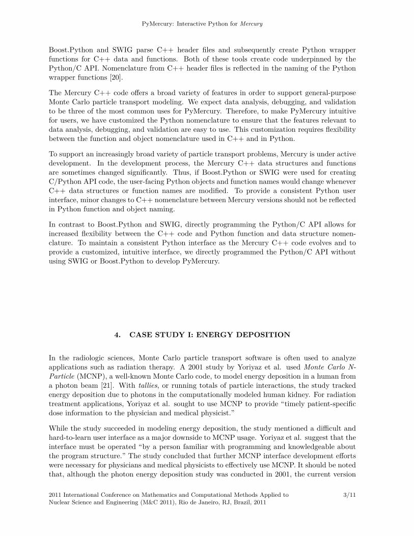
If the energy deposition study were conducted with Mercury, medical professionals could exploitruntime access to tallies through the PyMercury interactive interface. For example, with thePyMercury code in Figure 1, a medical professional could run Mercury until a user-specifiedthreshold of energy deposition has been reached. To accomplish this, the code in Figure 1accesses the energy deposition tally object with the PyMercury callmc.tally.tal["EnergyDeposition"]. (Note that all PyMercury functions begin with “mc” todenote Monte Carlo.) Then, the code uses the tally object’s getValue() function to request thetotal energy deposited by neutrons in the kidneys of the computer-simulated human figure. Withthe interactive Python interface, this code can be injected between iterations of the Mercuryparticle transport computation. For medical professionals, code like this could simplify theprocess of analyzing energy deposition in a computationally-modeled human figure.

energyTally = mc.tally.tal["EnergyDeposition"]

#Call at each cycle of Mercury executionif energyTally.getValue(Particle="Neutron", Cell="Kidneys") > 1e-6:

print "Neutron energy deposition to the kidneys reached threshold."

Figure 1: PyMercury code for tracking neutron energy deposition.

In short, this case study demonstrates that Python interactive runtime interfaces can improve theusability of the Monte Carlo code. In addition, since runtime tally access is not computationallyintensive, the PyMercury Python interface offers improved usability without contributing toperformance overhead.

5. CASE STUDY II: GEOMETRY VALIDATION

Many Monte Carlo particle transport applications use highly-tuned code for geometric calcula-tions [23] [2]. In the interest of fast application performance, optimizing the geometry code isoften of high priority in Monte Carlo code development. In addition to being critical to perfor-mance, geometry code can also be difficult to debug and to validate. A study of geometric setuptools describes the geometric setup as “typically the most challenging and error prone portionof a Monte Carlo model” [24]. With PyMercury, we demonstrate the applicability of Pythoninterfaces to validating geometry calculations in a Monte Carlo code.

In Mercury, a three-dimensional problem space is represented with combinatorial geometry (CG)spatial volumes, or cells [24]. Geometric setups for nuclear reactors, particle accelerators, andhuman figures can be represented in Mercury as collections of CG cells. For fast parallel perfor-mance, CG cell volume calculations are performed with highly optimized analytical calculationsor with adaptive mesh refinement (AMR) [25].

When new CG surfaces are implemented in Mercury, a “sanity check” volume calculation can aidin validating the analytic or AMR volume calculations for the new surfaces. To be meaningful,the “sanity check” calculation must be performed independently of the AMR code. Some toolsexist for testing geometry setups, such as VisIt [25] and Form Z to Monte Carlo (FZ2MC) [24].


4/11


These tools can provide visual representations of geometry setups in Monte Carlo simulations.However, testing and debugging with visual tools can be difficult to automate and often requirestime-consuming human input. While visual tools can be useful for fixing incessant bugs inMonte Carlo geometry setups, many geometry bugs can also be identified with automated testsimplemented with PyMercury. PyMercury offers all the tools necessary for creating simple,automated calculations with which to validate the analytical or AMR volume calculation code.

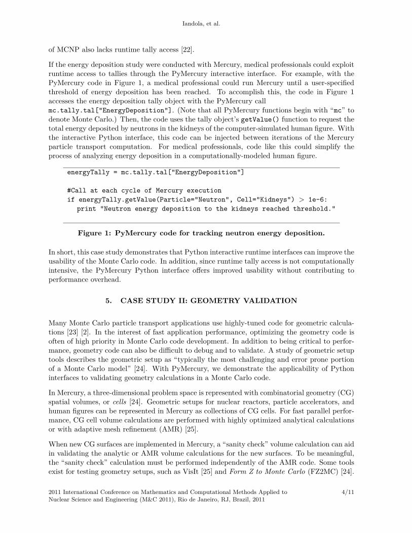
Figure 2: Hyberbolic Paraboloid calculated in Mercury; visualized in VisIt [25].

The Mercury development team has recently expanded Mercury’s library of CG cell shapes.Mercury now supports quadric surfaces such as the hyperbolic paraboloid shown in Figure 2.PyMercury is used to validate Mercury’s new, highly-optimized volume calculations for quadricsurfaces.

Mercury uses an analytical formula to calculate the volume of a hyperbolic paraboloid. The exactvolume of the hyperbolic paraboloid that we will study, can be computed from the integral:

ExactV olume =∫ 2

−2

∫ √x2+2

−√x2+2

(x2 − z2 + 2)dzdx

= 4 ∗ (3 ∗√

6 +ArcSinh(√

2))= 33.97874025


5/11

Iandola, et al.

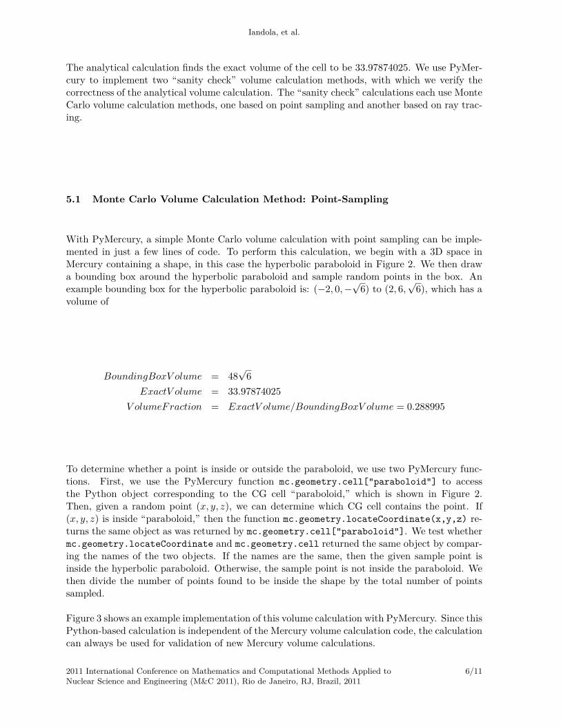
The analytical calculation finds the exact volume of the cell to be 33.97874025. We use PyMer-cury to implement two “sanity check” volume calculation methods, with which we verify thecorrectness of the analytical volume calculation. The “sanity check” calculations each use MonteCarlo volume calculation methods, one based on point sampling and another based on ray trac-ing.

5.1 Monte Carlo Volume Calculation Method: Point-Sampling

With PyMercury, a simple Monte Carlo volume calculation with point sampling can be imple-mented in just a few lines of code. To perform this calculation, we begin with a 3D space inMercury containing a shape, in this case the hyperbolic paraboloid in Figure 2. We then drawa bounding box around the hyperbolic paraboloid and sample random points in the box. Anexample bounding box for the hyperbolic paraboloid is: (−2, 0,−

√6) to (2, 6,

√6), which has a

volume of

BoundingBoxV olume = 48√

6ExactV olume = 33.97874025

V olumeFraction = ExactV olume/BoundingBoxV olume = 0.288995

To determine whether a point is inside or outside the paraboloid, we use two PyMercury func-tions. First, we use the PyMercury function mc.geometry.cell["paraboloid"] to accessthe Python object corresponding to the CG cell “paraboloid,” which is shown in Figure 2.Then, given a random point (x, y, z), we can determine which CG cell contains the point. If(x, y, z) is inside “paraboloid,” then the function mc.geometry.locateCoordinate(x,y,z) re-turns the same object as was returned by mc.geometry.cell["paraboloid"]. We test whethermc.geometry.locateCoordinate and mc.geometry.cell returned the same object by compar-ing the names of the two objects. If the names are the same, then the given sample point isinside the hyperbolic paraboloid. Otherwise, the sample point is not inside the paraboloid. Wethen divide the number of points found to be inside the shape by the total number of pointssampled.

Figure 3 shows an example implementation of this volume calculation with PyMercury. Since thisPython-based calculation is independent of the Mercury volume calculation code, the calculationcan always be used for validation of new Mercury volume calculations.


6/11


testCell = mc.geometry.cell["paraboloid"] #get geometric cell by nameBoxVolume = (xmax-xmin)*(ymax-ymin)*(zmax-zmin) #draw a bounding boxpointsFoundInCell = 0 #number of points found inside testCell

for i in xrange(numOfPoints):x = xmin + (xmax - xmin)*random.random()y = ymin + (ymax - ymin)*random.random()z = zmin + (zmax - zmin)*random.random()

#determine which cell the randomly generated coordinates are insidecellFoundByCoordinates = mc.geometry.locateCoordinate(x,y,z)if cellFoundByCoordinates.name == testCell.name:

pointsFoundInCell += 1

#volume of cell as determined by Monte Carlo trial.volume = (BoxVolume * pointsFoundInCell)/(numOfPoints)

Figure 3: Point Sampling Monte Carlo Volume Calculation with PyMercury.

To statistically evaluate the convergence of the point-sampling calculation, we vary the numberof points sampled or rays traced, n, within the cell’s bounding box. We run 1000 trials for fivevalues of n: 101, 102, 103, 104, and 105. For this test, we fix the processor count at 64 processors.

The mean of the point-sampling calculations converges to the analytically-calculated volume of33.97874025. As shown in Figure 4, the standard deviation, σ, is proportional to 1/

√n. The

standard deviation is approximately σ = 53/√n.

n samples mean σ σ√n |exact−mean|

1e+01 33.920534 16.6517 52.6573 5.8206e-021e+02 34.153333 5.4193 54.1932 1.7459e-011e+03 34.022119 1.6622 52.5621 4.3379e-021e+04 33.965413 0.5318 53.1824 1.3328e-021e+05 33.976479 0.1653 52.2728 2.2615e-03

Figure 4: Convergence for Point-Sampling Volume Calculation.

5.2 Monte Carlo Volume Calculation Method: Ray Tracing

To perform a volume calculation with ray tracing, we begin with the same setup as was used inthe point-sampling volume calculation. However, instead of sampling random points, we launchrays from random points along one face of the bounding box of a CG cell towards the oppositeface. We then calculate the fraction of the path length that was within the CG cell, comparedto the total path length traveled. This fraction approximates the volume fraction of the CG cellwithin its bounding box.

The ray-tracing volume calculation is easily enabled with PyMercury, which provides access tothe function nearestFacet(cell, x,y,z, α, β, γ). This function returns the distance to the


7/11

Iandola, et al.

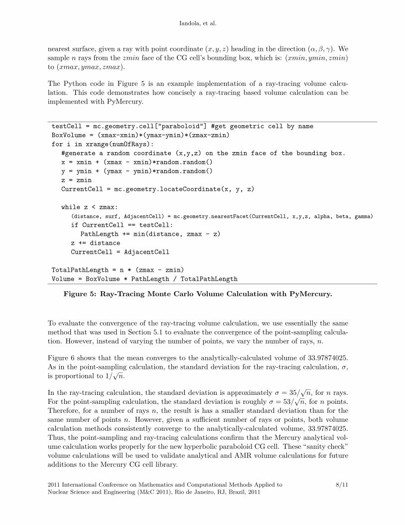
nearest surface, given a ray with point coordinate (x, y, z) heading in the direction (α, β, γ). Wesample n rays from the zmin face of the CG cell’s bounding box, which is: (xmin, ymin, zmin)to (xmax, ymax, zmax).

The Python code in Figure 5 is an example implementation of a ray-tracing volume calcu-lation. This code demonstrates how concisely a ray-tracing based volume calculation can beimplemented with PyMercury.

testCell = mc.geometry.cell["paraboloid"] #get geometric cell by nameBoxVolume = (xmax-xmin)*(ymax-ymin)*(zmax-zmin)for i in xrange(numOfRays):

#generate a random coordinate (x,y,z) on the zmin face of the bounding box.x = xmin + (xmax - xmin)*random.random()y = ymin + (ymax - ymin)*random.random()z = zminCurrentCell = mc.geometry.locateCoordinate(x, y, z)

while z < zmax:(distance, surf, AdjacentCell) = mc.geometry.nearestFacet(CurrentCell, x,y,z, alpha, beta, gamma)if CurrentCell == testCell:

PathLength += min(distance, zmax - z)z += distanceCurrentCell = AdjacentCell

TotalPathLength = n * (zmax - zmin)Volume = BoxVolume * PathLength / TotalPathLength

Figure 5: Ray-Tracing Monte Carlo Volume Calculation with PyMercury.

To evaluate the convergence of the ray-tracing volume calculation, we use essentially the samemethod that was used in Section 5.1 to evaluate the convergence of the point-sampling calcula-tion. However, instead of varying the number of points, we vary the number of rays, n.

Figure 6 shows that the mean converges to the analytically-calculated volume of 33.97874025.As in the point-sampling calculation, the standard deviation for the ray-tracing calculation, σ,is proportional to 1/

√n.

In the ray-tracing calculation, the standard deviation is approximately σ = 35/√n, for n rays.

For the point-sampling calculation, the standard deviation is roughly σ = 53/√n, for n points.

Therefore, for a number of rays n, the result is has a smaller standard deviation than for thesame number of points n. However, given a sufficient number of rays or points, both volumecalculation methods consistently converge to the analytically-calculated volume, 33.97874025.Thus, the point-sampling and ray-tracing calculations confirm that the Mercury analytical vol-ume calculation works properly for the new hyperbolic paraboloid CG cell. These “sanity check”volume calculations will be used to validate analytical and AMR volume calculations for futureadditions to the Mercury CG cell library.


8/11


n samples mean σ σ√n |exact−mean|

1e+01 33.951046 11.5092 36.3953 2.7694e-021e+02 33.755955 3.4363 34.3635 2.2278e-011e+03 33.954917 1.1544 36.5049 2.3823e-021e+04 33.974577 0.3678 36.7823 4.1634e-031e+05 33.981827 0.1099 34.7668 3.0864e-03

Figure 6: Convergence for Ray-Tracing Volume Calculation.

To summarize, PyMercury demonstrates that Python interfaces can simplify the testing ofgeometry-related components of Monte Carlo codes. Geometry code is critical to the correct-ness of Monte Carlo particle transport applications, and we expect Python interfaces to play anincreasingly significant role in the geometry validation process of numerous Monte Carlo codes.In addition to being used for debugging and validating geometry code, interactive Python codeand Python test scripts can potentially replace the majority of low-level code currently used fortesting Monte Carlo particle transport software.

6. CONCLUSIONS

Interactive Python interfaces are increasingly common in parallel scientific applications thatare primarily written in C, C++, and Fortran. Mixed-language codes using Python and C++can combine the performance advantages of C++ with the simplicity of the Python syntax.However, the Monte Carlo particle transport community has been slow to adopt mixed-languageprogramming models that combine low-level and high-level languages.

With PyMercury, we showed that connecting a Python interface with a Monte Carlo applica-tion can improve usability and simplify the process of validating the Monte Carlo code. Aswe demonstrated in Case Study I, PyMercury improves application usability during Mercuryruntime. As shown in Case Study II, PyMercury also simplifies the process of debugging andvalidating the Mercury code. PyMercury provides these benefits without contributing to per-formance overhead.

In summary, PyMercury illustrates the benefits of interactive Python and mixed-language pro-gramming for Monte Carlo particle transport applications. In the future, we expect mixed-language programming with interactive Python and a low-level language to be increasinglycommon among Monte Carlo applications.

ACKNOWLEDGEMENTS

The authors thank Laxmikant V. Kale, M. Scott McKinley, Brian Ryujin, Lila Chase, T.J.Alumbaugh, and Jonathan Walsh for providing expertise in parallel computing, mixed-language


9/11

Iandola, et al.

programming, and particle transport. This work was performed under the auspices of the U.S.Department of Energy by Lawrence Livermore National Laboratory under Contract DE-AC52-07NA27344.

REFERENCES

1. F.B. Brown, A.C. Kahler, G.W. McKinney, R.D. Mosteller, and M.G. White. MCNP5 +Data + MCNPX Workshop. Proc. of Joint International Topical Meeting on Mathematics &Computation and Supercomputing in Nuclear Applications (M&C + SNA 2007)., Monterey,CA, April 15-19, (2007).

2. B.L. Kirk. Overview of Monte Carlo radiation transport codes. Radiation Measurements.,45, pp. 1318-1322 (2010).

3. M.F. Sanner. Python: A Programming Language for Software Integration and Development.Journal of Molecular Graphics and Modeling., 17, pp. 57-61 (1999).

4. D.M. Beazley. Interfacing C/C++ and Python with SWIG. Proc. of 7th InternationalPython Conference., Houston, TX, November 10-13, (1998).

5. R. Procassini, et al. Verification and Validation of Mercury: A Modern, Monte Carlo ParticleTransport Code. Proc. of The Monte Carlo Method: Versatility Unbounded in a DynamicComputing World., Chattanooga, TN, April 17-21, (2005).

6. R. Procassini, et al. New Features of the Mercury Monte Carlo Particle Transport Code.Proc. of Joint International Conference on Supercomputing in Nuclear Applications andMonte Carlo (SNA + MC 2010)., Tokyo, Japan, October 17-21, (2010).

7. W. Gropp, E. Lusk and A. Skjellum. Using MPI: Portable Parallel Programming with theMessage Passing Interface. MIT Press, Cambridge, MA (1999).

8. T.J. Alumbaugh. Dynamic Languages for HPC at LLNL. Proc. of Virtual ExecutationEnvironments for Scientific Computing (VEESC 2010)., Arlington, VA, September 3-4,(2010).

9. R.A.A. Ince, R.S. Peterson, D.C. Swan, and S. Panzeri. Python for information theoreticanalysis of neural data. Frontiers in Neuroinformatics., 3 (2009).

10. F. Gioachin and L.V. Kale. Dynamic High-Level Parallel Scripting. Proc. of the 23rd IEEEInternational Parallel and Distributed Processing Symposium (IPDPS 2009)., Rome, Italy,May 23-29, (2009).

11. B. Thorne and R. Grasset. Python for Prototyping Computer Vision Applications. Proc. ofNew Zealand Computer Science Research Student Conference (NZCSRSC 2010)., Welling-ton, New Zealand, April 12-15, (2010).

12. P.J.A. Cock, et al. Biopython: freely available Python tools for computational and molecularbiology and bioinformatics. Bioinformatics., 25, pp. 1422-1423 (2009).

13. A.C. Calleja. Scripting a Large Fortran Code with Python. Proc. of First InternationalWorkshop on Software Engineering for High Performance Computing System Applications.,Edinburgh, Scotland, United Kingdom, May 24, (2004).


10/11


14. A. Ferrari, et al. Update on the Status of the FLUKA Monte Carlo Transport Code. 15thInternational Conference on Computing in High Energy and Nuclear Physics (CHEP 2006).,Mumbai, India, February 13-16, pp. 294-302 (2006).

15. V. Vlachoudis, et al. FLAIR: A Powerful But User Friendly Graphical Interface For FLUKA.Proc. of International Conference on Mathematics, Computational Methods, and ReactorPhysics (M&C 2009)., Saratoga Springs, NY, May 3-7, (2009).

16. B. Walker, J. Figgins, and J.R. Comfort. A Framework for Monte Carlo simulationcalculations in GEANT4. Nuclear Instruments and Methods in Physics Research Section A:Accelerators, Spectrometers, and Associated Equipment., 768, pp. 889-895 (2006).

17. G. van Rossum and F.L. Drake. Python/C API Manual - Python 2.6. CreateSpace,Paramount, CA, USA (2009).

18. D. Abrahams and R.W. Grosse-Kunstleve. Building Hybrid Systems with Boost.Python.C/C++ Users Journal. (2003).

19. D.M. Beazley. SWIG : An Easy to Use Tool for Integrating Scripting Languages with C andC++. Proc. of the 4th USENIX Tcl/Tk Workshop., Monterey, CA, July 10-13, (1996).

20. J. Generowicz, P. Mato, W.T.L.P Lavrijsen, and M. Marino. Reflection-Based Python-C++Bindings. Lawrence Berkeley National Laboratory., October 14, (2004).

21. H. Yoriyaz, M.G. Stabin, and A. das Santos. Monte Carlo MCNP-4B-Based Absorbed DoseDistribution Estimates for Patient-Specific Dosimetry. Journal of Nuclear Medicine., 42,pp. 662-669 (2001).

22. F.B. Brown, R.D. Mosteller, and A. Sood. Verification of MCNP5. Proc. of Nuclear Mathe-matical and Computational Sciences: A Century in Review, A Century Anew (M&C 2003).,Gatlinburg, TN, April 6-11, (2003).

23. W.S. Kiger III, A.G. Hochberg, J.R. Albritton, and T. Goorley. Performance Enhancementsof MCNP4B, MCNP5, and MCNPX for Monte Carlo Radiotherapy Planning Calculationsin Lattice Geometries. Proc. of Eleventh World Congress on Neutron Capture Therapy.,Waltham, MA, October 11-15, p. NEP-14 (2004).

24. B. Hackel, D. Nielsen, and R. Procassini. FZ2MC: A Tool for Monte Carlo TransportGeometry Manipulation. Proc. of International Conference on Mathematics, ComputationalMethods, and Reactor Physics (M&C 2009)., Saratoga Springs, NY, May 3-7, (2009).

25. M. O’Brien, R. Procassini, and K. Joy. Mercury + VisIt: Integration of a Real-TimeGraphical Analysis Capability Into a Monte Carlo Transport Code. Proc. of InternationalConference on Mathematics, Computational Methods, and Reactor Physics (M&C 2009).,Saratoga Springs, NY, May 3-7, (2009).

26. R. Procassini, M. O’Brien, and J. Taylor. Load Balancing of Parallel Monte Carlo TransportCalculations. Proc. of Mathematics and Computation, Supercomputing, Reactor Physicsand Nuclear and Biological Applications (M&C 2005)., Palais des Papes, Avignon, France,September 12-15, (2005).


11/11

PyMercury - Forrest Iandola

Documents

Transcript of PyMercury - Forrest Iandola