Putting Economics (Back) into Quantitative Models

VINEER BHANSALI 12

I am not an Economist. I am not even a union card holder in Finance, and accidentallyarrived on a Wall-Street trading desk via the back-door cracked open by the 1990 recessionin science. Now that I have had some experience trading and managing money, and alsoobserving a handful of very successful investors and some not so successful ones, and inbuilding models that have worked and failed, I have a few ideas on what kind of modelswork and what kind don’t work. The common thread that ties these ideas is that explicitrecognition and inclusion of the economics underlying the models is critical for their quality.Its not easy, but recent research by many in academia and industry has shown that indeedwe can make a fair bit of progress. (Ex)- physicists talking about putting economics backin finance - and you thought you had seen everything!

Somewhere along the way as we quants became more mathematically sophisticated andobtained faster processing power, the approximation and computational muscle that was ashort-cut took on a life of its own, largely at the expense of the economic common sensethat lies behind the purpose of investing - making superior excess risk-adjusted returns.The last twenty years have seen some serious financial debacles, and perhaps the nextgeneration of models will incorporate the errors of the previous generation as part of themodeling framework. Bjorn Borg, one of the greatest tennis players of all time was hiscoach’s exhibit on what not to do on the tennis court; especially not to use two handson the tennis racquet; until he started to win championships. Financial models need thesecond hand to make them better - not using economics from the very beginning as inputsinto the model is playing with one hand behind your back.

Models are assumed to operate in a theoretically ideal environment. When modeling thebehavior of an elephant in the jungle, a physicist makes the assumption that the elephantcan be thought of as a large sphere. Everything that follows will then depend on thisassumption, and hence it can be expected to fail under a wide range of conditions when theelephant is not really a sphere.

In the words of Myron Scholes, 3

We make models to abstract reality. But there is a meta-model beyond themodel that assures us that the model will eventually fail. Models fail becausethey fail to incorporate the inter-relationships that exist in the real-world.

At a recent conference of quants in the financial markets, Jack Treynor was asked whathe would recommend as a topic to the group of senior industry and academic participants

1PIMCO, 840 Newport Center Drive, Newport Beach, CA 92660, USA (e-mail:bhansali@pimco.com).Past performance is no guarantee of future results. This article contains the current opinions of theauthor but not necessarily those of Pacific Investment Management Company LLC. Such opinions are subjectto change without notice. This article has been distributed for educational purposes only and should notbe considered as investment advice or a recommendation of any particular security, strategy or investmentproduct. Information contained herein has been obtained from sources believed to be reliable, but notguaranteed. No part of this article may be reproduced in any form, or referred to in any other publication,without express written permission of Pacific Investment Management Company LLC. 2005, PIMCO.

2Presented as Plenary Session - Risk Magazines Annual Quant Congress, 2005, NY Nov. 8 and 9, 2005.3M. Scholes, speech given at the NYU/IXIS conference on Hedge Funds, New York, September 2005

who meet twice a year to discuss important issues in modeling. Somewhat reluctantly (sinceJack is a very modest person) said that he wished he had studies macroeconomics morecarefully, and that “macroeconomics” as a topic would be highly welcome, because so muchof actual policy and investment depends on it.

I will argue that incorporating economic principles; such as demand and supply, investorbehavior, preferences etc. from microeconomics, and monetary policy, macro aggregates,deficits, trade balances etc. from macroeconomics can help make our models more flexible,and hence more robust. Incentives drive the action of market participants, investors, andquantitative modelers. This approach to modeling is not pie in the sky. Recent work bymany 4 has shown that we can build better models without giving up the basic principlesthat form the foundations of arbitrage free pricing or the law of one price. Having economicsas the backdrop enables “better estimates of the distribution of future outcomes than asimplistic stochastic process of an unobserved factor estimated over a period of decades ”5.Models fail not because the math underlying them is wrong, but because because by blindlygoing to the risk-neutral framework we often misprice risk-premium, and hence mis-pricerisk. Emanuel Derman talked about neoclassical, behavioral, physical and mathematicalapproaches to model building. Incorporating economics leads to an approach which is theproper blend of all these - a real-world risk based approach to pricing and investing.

Why do we need economics in our models? Doesn’t risk neutral valuation make real-world probabilities irrelevant for pricing? Risk-neutral valuation argues theoretically thatif you can decompose the movement of any security into continuously tradable replicatingportfolios, and actually traded the replicating portfolios continuously, you can choose anyprobability measure you want. Its the “actual” part that causes problems and breakdownbetween theory and reality. There is no instantaneity in real markets. Economics, risk-aversion, preferences creep in. Even if you could overcome the technical difficulties, theapproach to model building that we have been taught might lack in some key non-technicalaspects; and the difference between investors who deliver returns with a good risk profileover multiple cycles and realizations of the real world, and those who don’t, might actuallybe explainable in terms of how their approach to investment explicitly incorporates theeconomic environment. So, I am not simply going to argue that Black-Scholes is incompletesince it assumes the wrong distributions, static volatility etc. Incorporating economicsexplicitly simply makes better models without throwing away any of the gains from ourwell-developed theoretical arbitrage free framework. It is possible to be arbitrage free,while at the same time stay in the world of common sense. There are successful academicswho have made lots of money as investors, and many of these have realized that modelframeworks stuck in static reality operate in a parallel world of spherical elephants; andusers of these models can be arbitraged by more realistic denizens of the financial jungle.Investment advisors still advocate standard friction-free idealized CAPM even though ithas been shown to be woefully inadequate - “Investors have realized frequently that theywere grossly misled by academics...for example, by advocating the holding of the marketportfolio of stocks, academics were basically marketing the stocks in the New York Stock

4The “classic” reference for the resurgent interest in this area is Ang, Andrew, and Monika Piazzesi,“A No-Arbitrage Vector Autoregression of Term-Structure Dynamics with Macroeconomic and Latent Vari-ables.”, Journal of Monetary Economics, Vol. 50, No. 4(2003), p 745.

5I would like to thank Brian Sack for this comment.

2

Exchange.” 6.Let us begin by discussing the main purposes of quantitative models, whether they are

reasonable, and how we can improve them by using economics. At the end of this discussion Iwill show a simple toy model that incorporates economics and arbitrage free concepts fromthe very beginning. I should mention that this is not the only possible implementation.Others have implemented other specifications. The value is really in the concept, not in theparticular mathematical form; though having a simple mathematical form simply makesanalysis more tractable.

1. Relevance for making money and managing risk

There are basically four (honest) ways to generate returns (we ignore the possibilityof front-running or using privileged information as an option). I will call them “profitmodes”:

(a) Taking factor risk exposures (macro)

(b) Intermediation (brokering)

(c) Liquidity and or risk transfer (insurance)

(d) Mispricing (arbitraging inefficiency)

Most money making enterprises are combinations of these modes. To make a modelrelevant to the particular combination of profit making modes, it has to be calibratedto the relevant combination of modes that is expected to yield excess returns for theinvestor selecting the combination. The economic environment is the backdrop withinwhich modes for profit are evaluated and models calibrated. A good example comesfrom option pricing models used on derivatives trading desks. Whether used for takingfactor exposures, intermediating, warehousing or arbitraging, the model developmentprocess works in the following sequence:

(a) Assume a distribution for the fundamental variables (for the standard libor mar-ket model forward rates are assumed lognormally distributed), and estimate theparameters using history and common sense as input,

(b) Generate probable paths of evolution,

(c) Fit remaining free parameters in the model to traded security prices,

(d) Price other securities with the model.

The framework as laid out is consistent for relative pricing, but because it has sub-stantial number of underlying distributional assumptions, it might not be equippedto automatically adapt as the underlying dynamics undergo a structural shift. Theseshifts have to be incorporated by hand to ensure that the model is well-calibratedfor what the model is designed to do. A case in point: the failure of many modelsas Japanese nominal rates dropped to zero over the last fifteen years. The lognormalframework would of course make it impossible for rates to fall below zero percent. Butzero percent floors indeed have been marketed and traded. A model that works well

6Sanford Grossman, speech at NYU/IXIS conference on Hedge Funds, 2005.

3

for long term investing and is designed to warehouse risks would fail miserably if it isused for high-frequency directional trading or arbitrage, and vice versa. Dealer desksmake money through the flow business - they only need models that can be locallycalibrated to today’s market, because tomorrow the position will be unloaded to an-other customer. For shorter holding periods, it does not make a big difference if themodel is improperly calibrated to the big picture. Hedge funds make money throughtaking residual risks - it does matter that the models they use are properly calibratedto possible episodes of missing liquidity. Mutual funds and insurance companies donot lever much, hence their risk taking necessarily reflects their ability to hold illiq-uid positions for longer periods. Hedge funds and mutual funds seemingly operate inthe same mode, but differ fundamentally in their ability to obtain funds with lowerhaircuts and for longer commitment periods. This financing difference makes all thedifference on how holding period returns are computed. Between the time of puttinga position on and taking it off the world can change; recalibration shocks should notforce an unwind of the position. Dealer desks and hedge funds operations are suited torisk-neutral and physical measures respectively because that’s the most appropriatemeasure for their investment objective.

It is critical that the fundamental variables in the model reflect observables, or exe-cutables. It is elegant to build models that can be described in terms of a small setof factors (principal components for interest rate models), but if a portfolio managercannot quickly translate the change in the market into simple combinations of marketinstruments, the models become irrelevant to practical investing.

2. Stability, analytical tractability and the ability to stress test

Exact solvability has forced many term structure and credit modelers to restrict theirattention to a subclass of models called affine models; with a limited set of prices ofbonds and swaps as inputs, but not their options as inputs, these models typicallydo not replicate the underlying dynamics of the yield curve and its volatility verywell. Partial technical victory is assumed to subsume reality. While these modelsprovide a nice sandbox within which to do thought experiments, and also spawnPh.D. theses, they lack fundamentally in the ability to capture the important nuancesof the market. For example, the evolution of the covariance of the term structure islargely undescribable in this framework. Good models would have rates and volatilitiesdescribed simultaneously since practitioners know that the shape of the yield curvealso reflects premium due to uncertainty.

Even if we could surmount the technical limitations of affine models using more so-phisticated, albeit numerical models, there are other assumptions that most analyticalmodels make which are harder to get around. Analytically tractable models are basedon assumptions of continuity, but the world is full of structural breaks. Most modelslean very heavily on the notion of stability by assuming stable distributions for thedynamics. After a hundred years of stochastic calculus this is all we really have towork with mathematically, since stable distributions and processes are easy to modeland solve. They are the harmonic oscillator of finance. But markets and policiesundergo rapid structural breaks. No avalanche is allowed in typical models until ithappens. Since most term structure models are based on the principle that long rates

4

are time averages of short rates plus risk premium, there is no way to account for thepossibility of structural breaks unless it is done right from the building block level.Again, as Scholes puts it - “shocks occur that stop time, and this gives us a chanceto recalibrate our old models to new data, or to incorporate new thinking into oldmodels; human capital becomes relevant.” I find it unsatisfactory that human capitalhas to bail out our models as frequently as it has.

To pursue this further, let’s discuss the basic building block for interest rate models -the short rate. Note that the Taylor rule (widely argued to be the Fed’s rate settingrule during the Greenspan era, at least) is specified as:

it = (r∗ − θ1π∗) + θ1(πt) + θ2(u∗ − ut) + πt. (1)

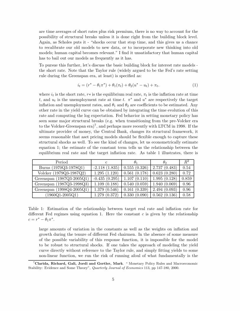
where it is the short rate, r∗ is the equilibrium real rate, πt is the inflation rate at timet, and ut is the unemployment rate at time t. π∗ and u∗ are respectively the targetinflation and unemployment rates, and θ1 and θ2 are coefficients to be estimated. Anyother rate in the yield curve can be obtained by integrating the time evolution of thisrate and computing the log expectation. Fed behavior in setting monetary policy hasseen some major structural breaks (e.g. when transitioning from the pre-Volcker erato the Volcker-Greenspan era)7, and perhaps more recently with LTCM in 1998. If theultimate provider of money, the Central Bank, changes its structural framework, itseems reasonable that aset pricing models should be flexible enough to capture thesestructural shocks as well. To see the kind of changes, let us econometrically estimateequation 1; the estimate of the constant term tells us the relationship between theequilibrium real rate and the target inflation rate. As table 1 illustrates, there is

Period c θ1 θ2 R2

Burns (1970Q3-1978Q1) -2.118 (1.835) 0.555 (0.326) 2.737 (0.483) 0.54Volcker (1979Q3-1987Q2) 1.295 (1.120) 0.561 (0.178) 0.623 (0.280) 0.72

Greenspan (1987Q3-2005Q1) -0.435 (0.295) 1.107 (0.110) 1.995 (0.128) 0.859Greenspan (1987Q3-1998Q3) 1.109 (0.188) 0.540 (0.059) 1.940 (0.069) 0.96Greenspan (1998Q4-2005Q1) 1.379 (0.546) 0.161 (0.339) 2.494 (0.093) 0.96

(1960Q1-2005Q1) 1.279 (0.372) 0.330 (0.090) 0.562 (0.136) 0.58

Table 1: Estimation of the relationship between target real rate and inflation rate fordifferent Fed regimes using equation 1. Here the constant c is given by the relationshipc = r∗ − θ1π

∗.

large amounts of variation in the constants as well as the weights on inflation andgrowth during the tenure of different Fed chairmen. In the absence of some measureof the possible variability of this response function, it is impossible for the modelto be robust to structural shocks. If one takes the approach of modeling the yieldcurve directly without reference to the Taylor rule, and simply fitting yields to somenon-linear function, we run the risk of running afoul of what fundamentally is the

7Clarida, Richard, Gali, Jordi and Gertler, Mark. “ Monetary Policy Rules and MacroeconomicStability: Evidence and Some Theory”, Quarterly Journal of Economics 113, pp 147-180, 2000.

5

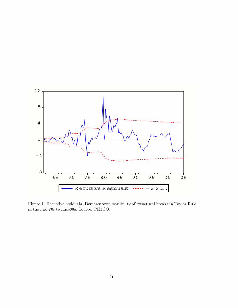
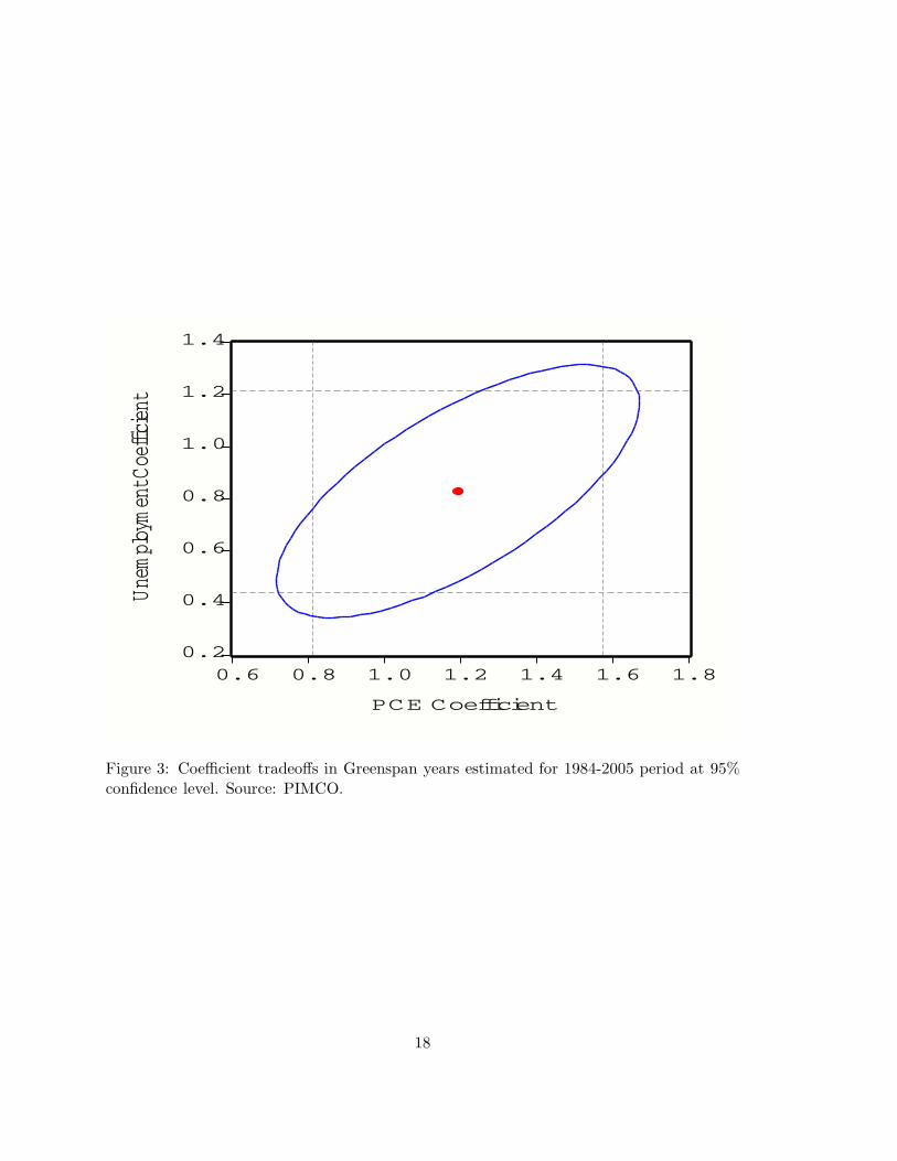
driving dynamics for the short rate. Figures 1,2 show the structural break, and figure3 shows the tradeoff between coefficients during the Greenspan years. Figure 4 showsthe difference in coefficient tradeoffs during different Fed chairmen tenures.

Let’s take a look at models for structured credit. For ease of computation, the currentstate of the art of credit modeling assumes a copula function to describe the jointbehavior of loss; quants know the limitation of the approach, but as of today there isno common benchmark model to improve upon the gross shortcomings of the copulaapproach. The Gaussian copula is to structured credit what the lognormal assumptionis to option valuation. The base correlation skew of copula based models is like thevol skew of options. The key simplification in the copula approach is provided by theassumption of a default correlation parameter which is an input. However, the defaultcorrelation that goes into the model is not directly observable. When Northwest andDelta entered bankrupty within minutes of each other in September, we saw defaultcorrelation in practice, and it was 1! No estimation devoid of ex-ante input wouldhave this as an input. When describing the reason for the simultaneous defaults, mostanalysts would use macroeconomic variables as the cause - underfunded pensions,falling revenues, competition, increased oil prices. It seems hard, if not impossible,to include the macro inputs as complex as these into one parameter. So we settle forcharge for the uncertainty by fitting prices to imply the value of the parameters. Weeven trade tranches assuming that they can be packaged together in an essentiallyarbitrage free way, which is just a wrong assumption unless liquid recovery productscan be traded. Figure 6 shows the actual and realized delta adjusted return of tranchesin the Spring. Not only was the hedge not a hedge in magnitude, for many tranches,the sign was wrong!

At the very least, if the copula model for trading default correlation has any value, itshould be possible to attribute portions of the default correlation to real life economicfactors. In other words, if the model is required to possess any depth, what is exoge-nous has to be made endogenous. Numerous smart proprietary trading desks maketheir living by constructing structures that take advantage of the lack of uniformityin modeling standards. Some recent progress has been made in this direction with-out giving up analytical tractability; for example, state contingent joint distributionof returns to describe comovement, instead of unconditional correlations, where thestates depend on macro scenarios.

Perhaps the most important reason for using simple, parametric models is that thesemodels can be solved and the parameters stress tested to obtain hedge ratios. Fortrading desks trained under the risk-neutral approach, the local hedge ratios, mark-to-market constraints, and running “flat” books can take a life unto itself. Thisapproach works well when markets are liquid and price discovery is easy. However,locally risk-neutral models fail horribly when securities are illiquid or markets areunder stress. The limitations of using risk-neutral pricing become all too obvious.The most perverse outcome is that the hedge ratios take on a life of their own; tohedge, underlying securities are traded. When the market hedge ratios are largeenough, the act of dynamic hedging can lead to the modification of the prices ofthe hedging securities in an amplifying feedback. When large enough in magnitude,

6

these models can actually lead to sytemic market distortions, such as the numerousmortgage debacles of the last decade, and perhaps even the crash of 1987. Anecdotally,the rapid rise of quantitative credit models has coincided with numerous proptietary“capital structure arb” desks and dedicated hedge funds. With Merton like modelingframework applied to credit and equity, a new theoretical connection has become all-too practical. Is falling equity volatility that has been accompanied with tighteningcredit spreads (see figure 8) a coincidence or a consequence of massive scale applicationof these sort of models?

But doing away with risk-neutrality is not a cure-all. Simple actual world Value atRisk models are notorious for failing when you need them most and for working greatwhen you don’t need them. The reasons are many - first, since most VaR modelsare based on historically estimated covariance matrices, so they simply cannot seestresses unless the covariance matrix is taken to its mathematically extreme values.To systematically take covariance matrices to logical extreme values, economic priorsand portfolio risks under those outcomes have to be built in right from the beginning.8

For example, a VaR model based on history alone would almost never capture episodeslike bull flattening, where yields and the steepness of the curve fall simultaneously.As many mortgage investors recently found out, valuation and risk models did verybadly in the 2004/2005 bull flattening episode. Hurricanes in Canada? Possible if youallow for parameters to take values under structural shocks.9 The risk model has to besimple enough to enable translation of envisioned outcomes into ranges of outcomesfor the risk factors.

3. Freedom from arbitrage

Models are approximations; demand and supply considerations are largely ignored.When we are unable to estimate the impact of clientele effects, we resort to the as-sumption of freedom from arbitrage to make the models work. With this approach, wehave seen some major technical breakthroughs in our time. Black-Scholes for optionsis one - and it depends on some simplifying assumptions regarding the underlyingdistributions. The copula approach is another, increasingly used for credit correlationproducts, and also depends on some simplifying assumptions regarding the form ofthe copula. However, even armed with the best arbitrage free quantitative modelspossible, experts can and do disagree. For example, in table 2 we show the OAS andduration numbers from a survey of the top MBS dealers on Wall Street for the samesecurity. 10 A levered derivative structure like an IO would magnify these errorseven further. Is it a wonder then that there are routine blowups in the mortgagederivative markets when there are large movements in underlying markets? It is oftenargued that you can reconstitute the collateral from the IO to PO, so given two ofthe three, the remaining one should trade at fair value. The problem is that liquidity,risk aversion and transaction constraints make it largely impossible for investors toreconstitute and arbitrage away the mispricing. So given the model risk, both IO’s

8See, for example, V. Bhansali and M.B. Wise, Forecasting Portfolio Risk in Normal and Stressed Markets,Journal of Risk 4, 2001.

9Hurricane Hazel hit Soutwestern Ontario on October 14, 1954.10I am grateful to the Pimco MBS desk for this data.

7

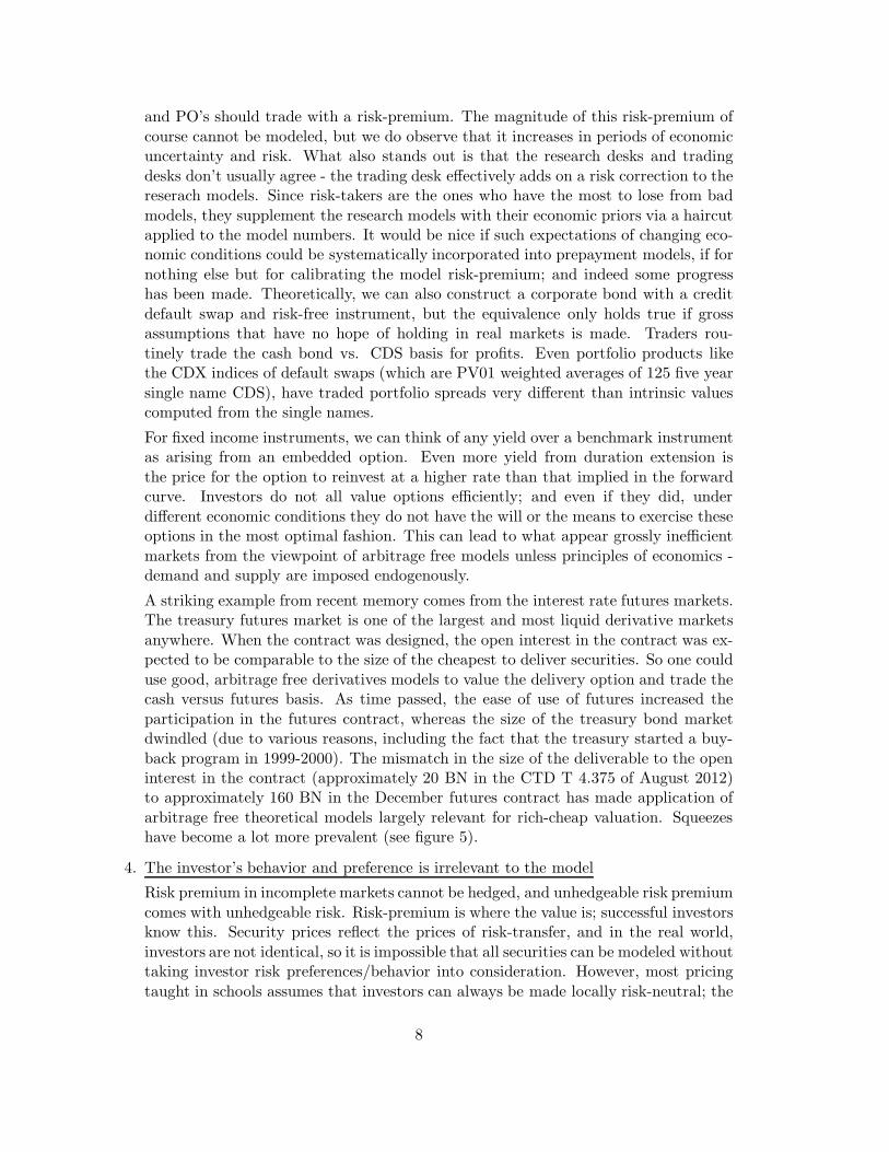
and PO’s should trade with a risk-premium. The magnitude of this risk-premium ofcourse cannot be modeled, but we do observe that it increases in periods of economicuncertainty and risk. What also stands out is that the research desks and tradingdesks don’t usually agree - the trading desk effectively adds on a risk correction to thereserach models. Since risk-takers are the ones who have the most to lose from badmodels, they supplement the research models with their economic priors via a haircutapplied to the model numbers. It would be nice if such expectations of changing eco-nomic conditions could be systematically incorporated into prepayment models, if fornothing else but for calibrating the model risk-premium; and indeed some progresshas been made. Theoretically, we can also construct a corporate bond with a creditdefault swap and risk-free instrument, but the equivalence only holds true if grossassumptions that have no hope of holding in real markets is made. Traders rou-tinely trade the cash bond vs. CDS basis for profits. Even portfolio products likethe CDX indices of default swaps (which are PV01 weighted averages of 125 five yearsingle name CDS), have traded portfolio spreads very different than intrinsic valuescomputed from the single names.

For fixed income instruments, we can think of any yield over a benchmark instrumentas arising from an embedded option. Even more yield from duration extension isthe price for the option to reinvest at a higher rate than that implied in the forwardcurve. Investors do not all value options efficiently; and even if they did, underdifferent economic conditions they do not have the will or the means to exercise theseoptions in the most optimal fashion. This can lead to what appear grossly inefficientmarkets from the viewpoint of arbitrage free models unless principles of economics -demand and supply are imposed endogenously.

A striking example from recent memory comes from the interest rate futures markets.The treasury futures market is one of the largest and most liquid derivative marketsanywhere. When the contract was designed, the open interest in the contract was ex-pected to be comparable to the size of the cheapest to deliver securities. So one coulduse good, arbitrage free derivatives models to value the delivery option and trade thecash versus futures basis. As time passed, the ease of use of futures increased theparticipation in the futures contract, whereas the size of the treasury bond marketdwindled (due to various reasons, including the fact that the treasury started a buy-back program in 1999-2000). The mismatch in the size of the deliverable to the openinterest in the contract (approximately 20 BN in the CTD T 4.375 of August 2012)to approximately 160 BN in the December futures contract has made application ofarbitrage free theoretical models largely relevant for rich-cheap valuation. Squeezeshave become a lot more prevalent (see figure 5).

4. The investor’s behavior and preference is irrelevant to the model

Risk premium in incomplete markets cannot be hedged, and unhedgeable risk premiumcomes with unhedgeable risk. Risk-premium is where the value is; successful investorsknow this. Security prices reflect the prices of risk-transfer, and in the real world,investors are not identical, so it is impossible that all securities can be modeled withouttaking investor risk preferences/behavior into consideration. However, most pricingtaught in schools assumes that investors can always be made locally risk-neutral; the

8

market is assumed to be complete and risk-aversion is assumed to be irrelevant becauseone can always transform to the risk-neutral measure. This is a huge assumptionthough. As time and time again we have witnessed, large, unhedgeable moves in themarket are routine, and even the best structured relative value trades expose theirabsolute risks.11

Locally hedgeable portfolios frequently cannot be created - as a matter of fact, locallyhedgeable portfolios are the exception rather than the rule (forget about globallyhedgeable portofolios; the only way to create them is to be a broker and lay off therisk completely or sell your position). The infamous CDX mezzanine versus equitytranche trade of the summer of 2005 illustrates this clearly. The correlation basedmodel assumes that tranches can be reconstituted to make up the underlying index,and comes up with a theoretical value based on this. However, when the underlyingeconomic environment suffered a shock with a possible auto default, securities behavedin exactly the opposite way than their theoretical deltas would have us believe theyshould, due to what would be called “irrational” deleveraging. So in practice we areleft with the problem of how to deal with risk-premium. Risk-premium is not constant.Far from it. Theoretically, the risk-premium is proportional to the covariance of theinvestor’s utility with the economic state of the world. In other words, assets that losetheir value when you are poor suffer a penalty (since when you are poor you value themarginal dollar more), and assets that gain in value in bad states of the world carrya premium (such as treasury bonds). In practice most consumers probably do notdo the life-cycle consumption maximization exercise, but rather look at the economythey can observe and expect. This is also why asset classes can quickly influenceeach other and lead to simultaneously lower expected returns across the cross-section.As Greenspan has remarked recently: “... low risk-free long-term rates worldwideseem to be one factor driving investors to reach for higher returns, thereby loweringthe compensation for bearing credit risk and many other financial risks over recentyears.”12. See figure 8 validating the assertion that uncertainty across markets canhave a high degree of correlation to lower rates of expected return. Market volatilityhas dived to low levels, but so has the volatility of economic variables such as inflationand GDP (figure 7). The Fed now moves in smaller steps. So to understand the sourcesof risk, and risk-premium, it is essential that the economics of the market environmentis understood. Assuming that assets will covary according to historical correlationsin all environments is a dangerous assumption - it throws out the understanding thatasset performance comes eventually from the need for the asset in a portfolio, notfrom a stand-alone pure value. This portfolio need for assets changes as the economic

11The key idea of risk-neutral pricing is that if a locally hedgeable portfolio can be created, then you canreplace the risk premium term with zero (or equivalently the discount rate with the risk-free rate). We canwrite the risk neutral probability in terms of the risky probability as arising from shifting the means

q̃ = N(N−1(q) + (µ̃ − µ)√

T ) (2)

where N represents the cumulative normal distribution and the physical probability is q̃ with risk-neutralprobability q.

12Remarks by Chairman Alan Greenspan Central Bank panel discussion To the International MonetaryConference, Beijing, Peoples Republic of China June 6, 2005

9

environment changes. The academic community tries to explain risk premium in thedefault swap market by comparing the risk-neutral reduced form intensities in thedefault swap market with the s-called “actual” probabilties implied by Merton orLeland-Toft models that have been industrialized by KMV and others. However, thisapproach is limited in its scope because it ignores that economic considerations (suchas the increased supply of investable cash), has gone preferentially into corporatebonds rather than equities.

5. The modeler should be irrelevant to the model

The variation in the modeler’s preferences on what short-cuts to take or what logicto follow in the creation of models, i.e. the value of the modeler’s human capitalis assumed to be largely irrelevant. It is no secret that in recent years the singlelargest impact on fixed income markets has been the growth of mortgages as an assetclass, and the commoditization of prepayment risk. Since the right to prepay is anoption for the homeowner, the investor in mortgages is short the prepay option. Nowassume that you are a large pension fund or agency trying to figure out how muchyour interest rate risk can change as prepayments change. The way you go aboutsolving the problem is to build a model to value the prepay option. Here’s the rub -the prepay option is priced using econometric inputs. In other words, homeowners donot prepay efficiently (and this is what presumably makes selling the option worth itto the investor), and the inefficiency of the prepay option exercise is quantified usingthe behavioral response of the collective homeowners in the past. But the behaviorin the past depends on a multitude of actual economic conditions (rate levels, creditconditions, demographics, unemployment rates, availability of housing, tax rates andbreaks, etc.). The hedge ratios for mortgages are thus related to economic inputsdirectly, and the model driven hedging activity, if large enough (as in Fall 2002), canimpact the prices of related securities and lead to a vicious feedback mechanism (needfor duration lead to buying of treasuries and falling yields lead to higher prepaymentsand more need for duration). People’s behavior changes as a response to the economicenvironment, so the models have to be able to capture this. How will a collapse ofhousing in California, were it to happen, affect risk-premia given that homeownersare buying homes essentially on their credit card? 13 Experts can disagree! We stresstested a number of models on their essential inputs for the same econometric variables,and found that the response of the models to the same set of inputs was very different.In other words, two modelers working across the street from each other, with the sameinputs and same training in Finance come up with very different models. There ismore art than science.

6. Price should reflect Value

This assumption is frequently violated. The following quote from none other thanAdam Smith jumps to mind:14

The things that have the greatest value in use have frequently little or novalue in exchange; and, on the contrary, those which have the greatest value

13Recent structures such as option ARMs has made this metaphor a reality.14Adam Smith, “The Wealth of Nations”, Book 1, Ch. 4 (1776).

10

Dealer Treasury OAS Libor OAS OAD (Research) OAD (Trading Desk)Lehman 26 3 4.8 4.6Goldman 81 34 4.6 4.0

Greenwich Capital 36 17 4.0 4.0CSFB 52 18 6.1 4.4

Salomon 51 16 5.2 4.4Morgan Stanley 52 29 5.0 4.2Bank of America 64 25 4.2 4.5

UBS 44 20 4.9 4.7Countrywide 107 50 5.1 4.1JP Morgan 54 23 6.1 4.1

Merrill 52 21 5.0 4.1Bear 65 21 5.3 4.3

Average 57 23 5.0 4.3Range 81 47 2.1 0.6Min 26 3 4.0 4.0Max 107 50 6.1 4.7

Table 2: FNMA 5.0% 30 Year Passthrough Option Adjusted Spreads and Option AdjustedDurations as of May 05, 2003. Source: PIMCO survey.

in exchange have frequently little or no value in use. Nothing is more usefulthan water; but it will purchase scarce any thing: scarce anything can behad in exchange for it. A diamond, on the contrary, has scarce any valuein use; but a very great quantity of other goods may frequently be had inexchange for it.

It is relatively easy to create a model to justify the price of a security without referenceto the economic environment, since in equilibrium demand and supply match. Itis harder to create a model to justify the value of a security. Even for the mostliquid securities, there is one price, but different values for different investors. OnSeptember 26th, Goldman Sachs issued 30 year tax exempt liberty bonds at a yield ofapproximately 4.59 % when 30 year treasuries were at 4.50 %. For a taxable investorthis yield may or may not be absolutely attractive (grossed up yield of almost 7%)given that we were at historically low levels in yields globally. On a relative basis,versus treasuries, this implied a higher than 100 % ratio, i.e. an implied term taxrate of zero percent without adjusting for credit. So on a relative basis one would saythat the deal was immensely attractive for a crossover taxable buyer. But implicit inthe valuation, both absolute and relative, is a view - for absolute buyers that such alow yield is justified because it locks in a 4.59 % yield for 30 years on a tax-exemptbasis, which would be justified if inflation falls. Since the tax risk cannot be hedged, iftaxes go up this would also turn out to be a good investment relative to a governmentbond at a lower yield. But people are buying taxable treasuries over the munis atthe same time. Does the buyer of the muni who is short the tax option deserve so

11

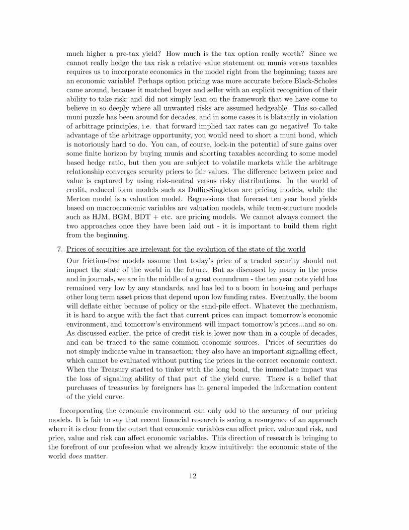
much higher a pre-tax yield? How much is the tax option really worth? Since wecannot really hedge the tax risk a relative value statement on munis versus taxablesrequires us to incorporate economics in the model right from the beginning; taxes arean economic variable! Perhaps option pricing was more accurate before Black-Scholescame around, because it matched buyer and seller with an explicit recognition of theirability to take risk; and did not simply lean on the framework that we have come tobelieve in so deeply where all unwanted risks are assumed hedgeable. This so-calledmuni puzzle has been around for decades, and in some cases it is blatantly in violationof arbitrage principles, i.e. that forward implied tax rates can go negative! To takeadvantage of the arbitrage opportunity, you would need to short a muni bond, whichis notoriously hard to do. You can, of course, lock-in the potential of sure gains oversome finite horizon by buying munis and shorting taxables according to some modelbased hedge ratio, but then you are subject to volatile markets while the arbitragerelationship converges security prices to fair values. The difference between price andvalue is captured by using risk-neutral versus risky distributions. In the world ofcredit, reduced form models such as Duffie-Singleton are pricing models, while theMerton model is a valuation model. Regressions that forecast ten year bond yieldsbased on macroeconomic variables are valuation models, while term-structure modelssuch as HJM, BGM, BDT + etc. are pricing models. We cannot always connect thetwo approaches once they have been laid out - it is important to build them rightfrom the beginning.

7. Prices of securities are irrelevant for the evolution of the state of the world

Our friction-free models assume that today’s price of a traded security should notimpact the state of the world in the future. But as discussed by many in the pressand in journals, we are in the middle of a great conundrum - the ten year note yield hasremained very low by any standards, and has led to a boom in housing and perhapsother long term asset prices that depend upon low funding rates. Eventually, the boomwill deflate either because of policy or the sand-pile effect. Whatever the mechanism,it is hard to argue with the fact that current prices can impact tomorrow’s economicenvironment, and tomorrow’s environment will impact tomorrow’s prices...and so on.As discussed earlier, the price of credit risk is lower now than in a couple of decades,and can be traced to the same common economic sources. Prices of securities donot simply indicate value in transaction; they also have an important signalling effect,which cannot be evaluated without putting the prices in the correct economic context.When the Treasury started to tinker with the long bond, the immediate impact wasthe loss of signaling ability of that part of the yield curve. There is a belief thatpurchases of treasuries by foreigners has in general impeded the information contentof the yield curve.

Incorporating the economic environment can only add to the accuracy of our pricingmodels. It is fair to say that recent financial research is seeing a resurgence of an approachwhere it is clear from the outset that economic variables can affect price, value and risk, andprice, value and risk can affect economic variables. This direction of research is bringing tothe forefront of our profession what we already know intuitively: the economic state of theworld does matter.

12

So, how do we properly put economics (back) into models? I propose one, not theonly possible, framework. Arguably, the framework is better adapted for models that areused for extracting systematic alpha. We begin by translating economic priors into possibleeconomic scenarios and the realization of the factors. For example, typically, but not always,low inflation and low GDP is associated with low interest rate levels and relatively flat yieldcurves. When pricing a credit risk-free security, the arbitrage free price can be compared orsupplemented with pricing obtained by the risk premia of these factors on the security. Ifunder shocks of the factors a so-called arbitrage free package yields non-zero excess returns,it has to hold true that the risk-neutral price is wrong, or there are hidden factors, or thereare risk-free profit opportunities.

• We can start by defining risk exposures in terms of specific factors. For instance,duration, curve exposure, spread exposures of various kinds, and structural compo-nents such as the magnitude of embedded volatility sale and the static aspects, suchas roll-down in the curve. For each of these factor exposures, we obtain factor riskpremia. For packages that allow factor risk-premia to be hedged out, we can priceusing the arbitrage free approach. Our model is general enough to have the economiccontent incorporated right from the beginning.

• Depending on our outlook of the world and the expected variation in risk premia,certain sources of risk are better than others at different times. Whenever we expectto be able to earn high risk premia in a sector, we overweight that sector/security.For example, the term-premium is the premium that is earned by increasing duration.To quantify the term-premium content of the yield curve, we build models that cansimultaneously extract the term premium from the whole yield curve.

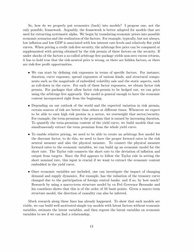
• To enable relative pricing, we need to be able to create an arbitrage free model forthe discount factor; to do this, we need to have the proper forward rates in the riskneutral measure and also the physical measure. To connect the physical measureforward rates to the economic variables, we can build up an economic model for theshort rate. The Taylor rule connects the short rate to the deviation of inflation andoutput from targets. Since the Fed appears to follow the Taylor rule in setting theshort nominal rate, this input is crucial if we want to extract the economic contentembedded in the yield curve.

• Once economic variables are included, one can investigate the impact of changingdemand and supply dynamics. For example, has the valuation of the treasury curvechanged due to the participation of foreign central banks; and if so, by how much?Research by using a macro-term structure model by ex Fed Governor Bernanke andhis coauthors shows that this is of the order of 50 basis points. Given a macro termstructure model, the direction of causality can also be inferred.

Much research along these lines has already happened. To show that such models areviable, we can build well-motivated simple toy models with latent factors without economicvariables, estimate the latent variables, and then regress the latent variables on economicvariables to see if we can find a relationship.

13

Let us build a quantitative term-structure model with economic content. Our approachwill be to build a well-motivated term structure model that is based in economics, estimatethe parameters in the model using market data (in an arbitrage free way), and then pickrelevant economic variables that are related to the latent variables by regression. Figure 10shows the key economic variables we will use - the inflation rate, real GDP, current accountdeficit as a percent of GDP, and the difference in the ten year and one year treasury ratesas a proxy for the term premium:

A general form of a two factor latent variable model is given by

dx = −µx(x − θx) dt + σx dwx

dy = −µy y dt + σy dwy

dz = k(x + y − z) dt

We can think of z as the instantaneous short rate, with fit results in figure 11. We canthink of x as related to inflation, and θx as the long term target for this variable.

Since the change in z is related to the diffence from the sum of x and y, it is temptingto identify these variables with the inflation and GDP gaps as in the Taylor rule and thedifference equation for z as the Taylor rule. The benefit of this specification is that we cannow bring in the machinery for solving for zero coupon bond prices and yields using:

P (t, T ) = Et[e−

∫ T

tz(α)dα] = e−y(T−t) (3)

which can be solved in closed form. Now that we have an analytical model for the discountfactors, we can fit the model to the term structure every day. Going back to 1960, we dothis exercise and obtain the estimated values of the parameters and variables of interest(see figure 12). Now we can try combinations of economic variables that correlate wellwith these estimated parameters. By construction, the structural changes in the “Taylorrule” are transmitted across the yield curve via the latent factors x and y. Figure 13shows that θx fits well with the inflation rate (plus some premium), and figure 14 showsthe dependence of the factor y on the slope of the yield curve (curve risk -premium). 15

Since the inflation risk factor is best expressed in terms of duration risk, and the curverisk-premium is best expressed in terms of yield curve steepening or flattening exposure,now we have a methodology to connect macro variables with risks of securities to thesemacro factors in an arbitrage free way (we simply compute the sensitivity with respect tothe factors for every credit risk free bond using the model).

We can also investigate the impact of the mushrooming US current account deficit byadding in the current account deficit as a percent of GDP to the regression for the long terminflation rate θx. As expected and shown in figure 15, we find that the market implied longterm inflation expectations have been kept much lower than they would have; For very longhorizons, long term inflation expectations could be almost two percent higher (difference offitted residuals in the model with and without the current account deficit as an explanatoryvariable).

Now that we see that economic variables have good explanatory power for the latentvariables, there is no reason why we should not build the economic variables into the model

15I would like to thank Wendong Qu of Pimco for collaboration on the implementation.

14

right from the beginning; in other words, one could argue that before fitting to the yieldcurve and security prices, we should constrain the ranges of the parameters and factorsusing our economic priors. In a sense, when we specify the model to have two sources ofuncertainty, plus policy, we are already imposing economics, i.e. we know from experi-ence that yield curve fluctuations can be described by at most three factors, and in mostcircumstances, by two factors. We also know that credit free fixed income securities arepredominantly determined by inflation (and inflation expectations), Fed behavior and risk-premium. So a simple, economically well-specified model is better suited to fit the marketthan a very general model that has little to do with the real-world in its specification. Anadvantage of such a model is also that the effect of the yield curve on the macroeconomy,as well as the effect of the macroeconomy on the yield curve can be estimated. The modelis efficient enough to stress test with. We have also explored an extension where creditrisk, prepayment risk and tax risk is introduced into the model explicitly from the startwith stochastic intensities correlated to macro factors. We can throw in all relevant eco-nomic variables into the mix right from the beginning and estimate a no arbitrage vectorautoregression in the spirit of Ang and Piazzesi (and others). Minimization of fitting errorsthen picks out the relevant economic variables. Due to the simultaneity of the market andeconomic variables, the impulse response functions show the impact of each set of variablesinto subsequent realizations of the others. The results appear promising.

We have systematically tried to put some economics back into models, at least a littlebit of economics. Much remains to be done. I would like to thank readers of initial drafts ofthis paper, and participants at Risk’s Quant Congress (2005) for listening to the talk andtheir followup questions.

15

-8

-4

0

4

8

12

65 70 75 80 85 90 95 00 05

Recursive Residuals – 2 S.E.

Figure 1: Recursive residuals. Demonstrates possibility of structural breaks in Taylor Rulein the mid 70s to mid-80s. Source: PIMCO.

16

-40

-20

0

20

40

60

80

100

65 70 75 80 85 90 95 00 05

CUSUM 5% Significance

Figure 2: Cumulative Sum Test for testing for structural breaks. Demonstrates structuralbreak in Taylor rule in 1980. Source: PIMCO.

17

0.2

0.4

0.6

0.8

1.0

1.2

1.4

0.6 0.8 1.0 1.2 1.4 1.6 1.8

Unem

ploym

entC

oeffic

ient

PCE Coefficient

Figure 3: Coefficient tradeoffs in Greenspan years estimated for 1984-2005 period at 95%confidence level. Source: PIMCO.

18

0.5 1 1.5 2 2.5 3Π*

-2

-1

1

2

3r*

Full Sample 1960-2005

Greenspan 1997-2005

Greenspan 1987-1997

Greenspan 1987-2005

Volcker 1979-1987

Burns 1970-1978

Figure 4: Tradeoff of PCE target and Real Rate Target in Era of Different Fed Chairmen.Source: PIMCO.

19

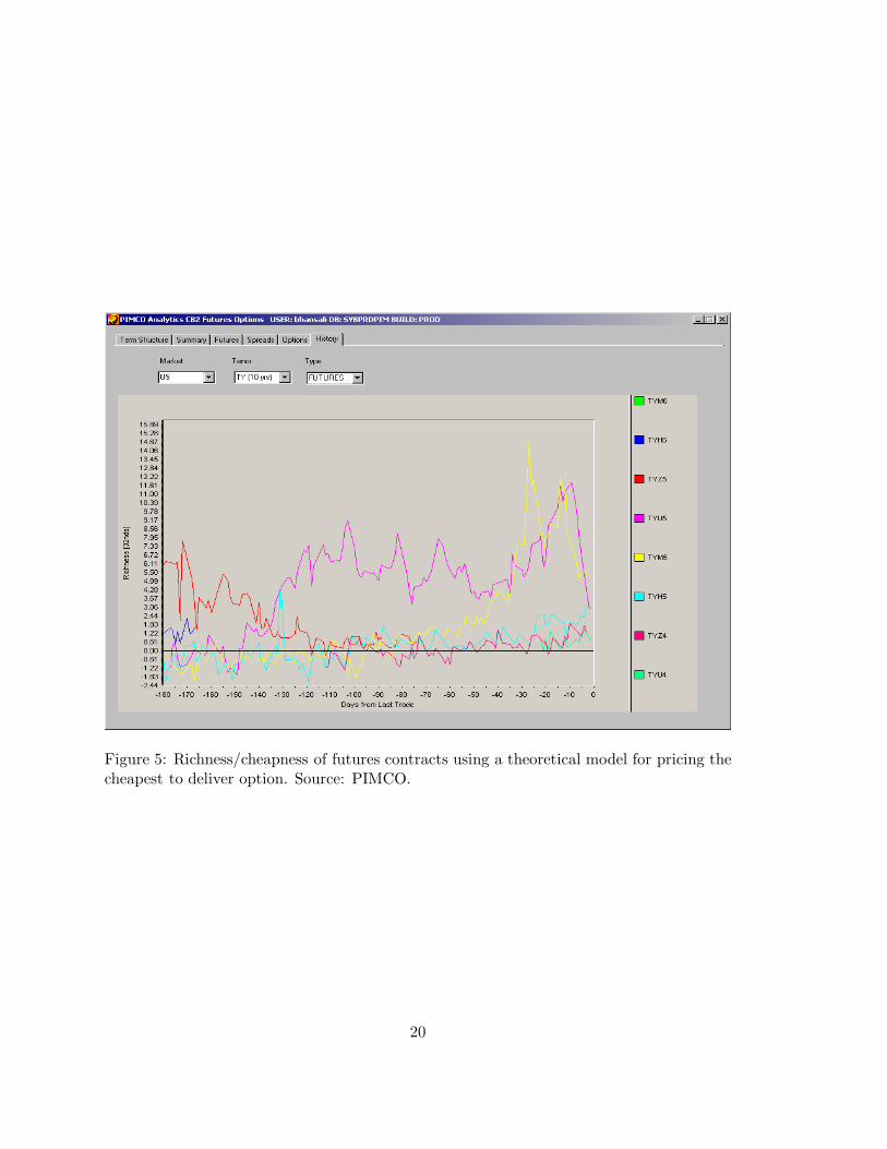
Figure 5: Richness/cheapness of futures contracts using a theoretical model for pricing thecheapest to deliver option. Source: PIMCO.

20

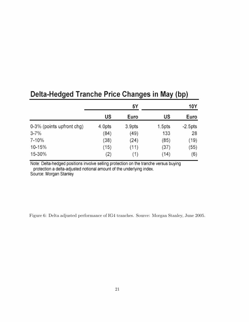
Figure 6: Delta adjusted performance of IG4 tranches. Source: Morgan Stanley, June 2005.

21

Figure 7: Inflation Rate and Inflation Volatility. Source: PIMCO.

22

Figure 8: VIX and Corporate Spreads. Source: Lehman Brothers.

23

Figure 9: Asset Excess Return Performance and Correlation to overall bond market as rep-resented by the Lehman Brothers Aggregate over five years. Source: PIMCO. Hypotheticalexample for illustrative purposes only. No representation is being made that any account,product, or strategy will or is likely to achieve profits, losses, or results similar to thoseshown. Hypothetical or simulated performance results have several inherent limitations.Unlike an actual performance record, simulated results do not represent actual performanceand are generally prepared with the benefit of hindsight. There are frequently sharp differ-ences between simulated performance results and the actual results subsequently achievedby any particular account, product, or strategy. In addition, since trades have not actuallybeen executed, simulated results cannot account for the impact of certain market risks suchas lack of liquidity. There are numerous other factors related to the markets in general orthe implementation of any specific investment strategy, which cannot be fully accounted forin the preparation of simulated results and all of which can adversely affect actual results.

24

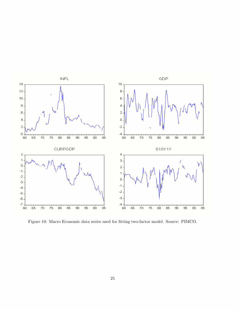
Figure 10: Macro Economic data series used for fitting two-factor model. Source: PIMCO.

25

Figure 11: Fed Funds Rate and z. Source: PIMCO.

26

Figure 12: Model Fits using only 1y, 3y, 5y, 10y treasuries as input. Source: PIMCO.

27

Figure 13: Model implied long term inflation rate regressed against actual inflation. Regres-sion equation θx = 4.868 + 0.619 ∗ INFL yields r2 of 0.46, with infl t-stats = 11.9. Source:PIMCO.

28

Figure 14: Second factor y versus economic and market variables. Regression equationy0 = −0.14− 0.0422 ∗ GDP − 0.00579 ∗ INFL − 0.667 ∗ (10Y − 1Y ). Only the slope factor10Y −1Y is significant. This indicates that the strongly mean reverting second factor mightbe more correlated to risk-premia and preferences than to economic cycles. Regressionsagainst market volatility indicators also show a high correlation of the second factor. Source:PIMCO.

29

Figure 15: Long term inflation expectations implied by term structure model regressedagainst actual inflation rates and current account deficit. Regression equation θx = 4.13 +0.687 ∗ INFL− 0.387 ∗CURPGDP, where t-stats on inflation rate equal 13, and on currentaccount deficit equal 5, so both variables are significant. Regression r2 = 0.54. Source:PIMCO.

30