Putting a Vortex in Its Place

Chris Snyder National Center for Atmospheric Research

Introduction

Data assimilation spanning a range of scales is difficult---a central unsolved problem in assimilation/state estimation

Hurricanes are an obvious example– Large-scale “steering” flow– Axisymmetric vortex– Asymmetric structure; rain bands– Convective elements, eye-wall details, …

Introduction

Importance of remotely sensed observations– Indirect; instrument does not measure model variables– Patchy in time and space

Also special, in-situ observations– Reconaissance flights provide position and intensity of

vortex

Themes

1. Initializing forecast/simulation model with vortex in correct location– Two scales: “environment” and vortex

2. Monte-Carlo (ensemble) methods for DA

Bogussing

• ICs for hurricane forecasts often involve some form of bogussing

• A simple, empirical approach to intializing hurricane vortex– Obs of intensity, size of vortex (e.g. from reconnaisance

flights) – Use these to determine parameters in analytic, axisymmetric

model of vortex … a “bogus” vortex– Information from bogus vortex inserted into ICs at observed

location of vortex

• Operational (NHC/GFDL) scheme1. Remove existing vortex from ICs2. Spin up vortex in an axisymmetric model, constraining low-level

winds to match those from specified bogus vortex3. Add axisymmetric vortex to ICs at observed location

A Simple 2D “Hurricane” Experiment

• 2D (barotropic) vorticity dynamics• (2400 km)2, doubly periodic domain• Strong vortex (80-km radius) embedded

in large-scale turbulent flow• Construct 31 ICs with small disp.s of

vortex and small diff.s in large scale 30 ensemble members + 1

“true”/reference state

10-4 s-1

A Simple 2D Experiment (cont)

t=24h 91 km

127 km

Position Errors in Hurricane Data Assimilation

• Errors in large scales produce wind errors local to vortex, and thus position/track errors

• Vortex intensity and structure also influence track and can lead to position errors

Resulting difficulties for data assimilation:• Influence of obs depends strongly on presence,

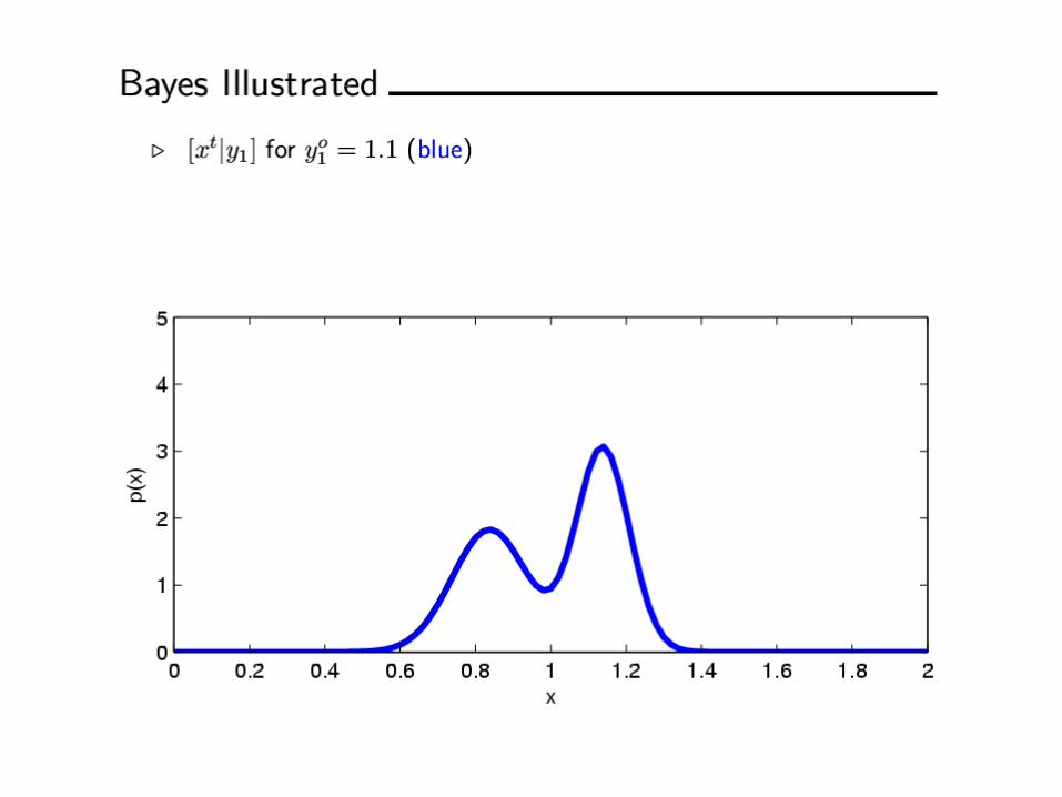
location of vortex • Even small displacements of vortex imply non-

Gaussian pdfs

Most practical DA schemes assume Gaussian prior with stationary, isotropic covariances

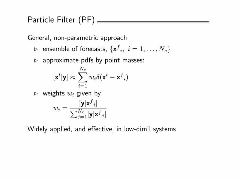
PARTICLE FILTER 1

PARTICLE FILTER 2

PARTICLE FILTER 3

PARTICLE FILTER 3

Other Non-Gaussian Assimilation Schemes

• 4D variational methods– Assume Gaussian prior and observation errors– Compute maximum likelihood estimate given obs in time

interval– Nonlinear minimization in many variables

• Methods based on “alignment” or “distortion”– Assume prior is known function of uncertain spatial

coords– E.g. suppose = (x + x, y + y), with x, y Gaussian– Lawson and Hansen (2004), Ravela et al. (2007)

Assimilation of Position Observations

• Wish to avoid difficulties associated with large position errors

• Geostationary satellites provide vortex position almost continuously in time

• Assimilating such obs should limit position errors in analysis

http

://c

imss

.sse

c.w

isc.

edu/

trop

ic/a

rchi

ve/m

onta

ge/a

tlant

ic/2

004/

IVA

N-t

rack

.gif

Details of Position Assimilation

• Need operator that returns vortex position given model fields, e.g., location of minimum surface pressure

• For small, Gaussian displacements, errors are Gaussian with covariances related to gradient of original field(x + x, y + y) - (x, y) (x, y)

• If position obs are accurate and frequent, can assimilate with a linear scheme

Ensemble Kalman Filter (EnKF)

• Estimates/models of forecast and obs. pdfs are crucial to DA.

• EnKF uses sample (ensemble) estimates

• EnKF considers only 1st, 2nd moments---linear scheme

EnKF Analysis Equations

• Assimilate obs serially (one at a time)• Given single obs y, any state variable x is

updated viaxa = xf + k ( y - yf ),

where yf = Hxf,

k = cov( xf, yf ) / ( var(yf ) + 2 ) .Both cov( xf, yf ) and var(yf ) are sample

(ensemble) estimates• Loop over state variables, loop over

observations• For large ensembles, converges to KF (or BLUE)• No adjoint or minimization algorithm required.

2D Experiment Revisited

• 2D (barotropic) vorticity dynamics• (2400 km)2, doubly periodic domain• Strong vortex (80-km radius) embedded

in large-scale turbulent flow• Construct 31 ICs with small disp.s of

vortex and small diff.s in large scale 30 ensemble members + 1

“true”/reference state

• Simulate obs of vortex position with random error

• Assimilate 1-hourly obs with EnKF

Chen, Y. and C. Snyder, 2007: Assimilating vortex position with an ensemble Kalman filter. Mon. Wea. Rev., in press.

10-4 s-1

2D Experiment Revisited

t=24h 91 km

127 km

Without assimilation With assimilation

Have also explored assimilation of intensity and shape of vortex

Experiments with WRF/DART

• WRF -- Weather Research and Forecasting model • DART -- Data Assimilation Research Testbed:

http://www.image.ucar.edu/DAReS/DART/• 36 km horizontal resolution, 35 vertical levels• 26/28 ensemble members• Ensemble initial and boundary conditions are generated

by perturbing GFS(AVN) analysis/forecast with WRF-VAR error statistics

• Assimilated observations: – hurricane track (center position and minimum sea level pressure

from NHC advisories)– Satellite winds (3% available observations)

• Compare forecasts initialized from the EnKF mean analysis and from the GFS analysis

Hurricane Ivan 2004

– 36-km horizontal resolution, 28 ensemble members– Assimilate position, intensity and satellite winds every 3h for a total of 24h– Compare forecasts initialized from the EnKF analysis and from the GFS analysis

Hurricane Ivan 2004

– 36-km horizontal resolution, 28 ensemble members– Assimilate position, intensity and satellite winds every 3h for a total of 24h– Compare forecasts initialized from the EnKF analysis and from the GFS analysis

Hurricane Ivan 2004

– 36-km horizontal resolution, 28 ensemble members– Assimilate position, intensity and satellite winds every 3h for a total of 24h– Compare forecasts initialized from the EnKF analysis and from the GFS analysis

Hurricane Katrina 2005

– Analysis: • 36-km horizontal resolution, 26 ensemble members• Assimilate position, intensity, and satellite winds every hour for a total of 12 hours

– Forecasts:• Compare forecasts initialized from the EnKF analysis, from the GFS/AVN forecasts and from GFDL analysis at 36-km and 12-km

resolutions

36-km 12-km

Hurricane Rita and Ophelia 2005

– 36-km horizontal resolution, 26 ensemble members– Assimilate position, intensity, and satellite winds every hour for a total of 12 hours– Compare forecasts initialized from the EnKF analysis and from the GFS/AVN forecasts.

Typhoon Dujuan 2003

– 45-km horizontal resolution, 28 ensemble members– Assimilate position, intensity, satellite winds, and GPS refractivity for 1 day or

2.5 days– Compare forecasts initialized from

• EnKF analysis• WRF 3DVAR analysis (3DVAR, cycling for 2.5 days)• GFS analysis (3DVAR-non)

Forecast time (day)

Increments to Vortex Structure

RITA at 2005-09-20-23Z

RITA 2005-09-20-23Z Center Lat. (oN) Center Lon. (oW) Mini. SLP(mb)

Observation (error) 24.00 (0.3) -82.20 (0.3) 973.0 (5.0)

Prior mean (spread)

23.85 (0.24) -82.33 (0.23) 988.6 (2.0)

Posterior mean (spread) 23.89 (0.15) -82.29 (0.18) 986.5 (2.0)

Vortex Spin-up

6-h Accumulated Precipitation

Katrina 2005, 12-km

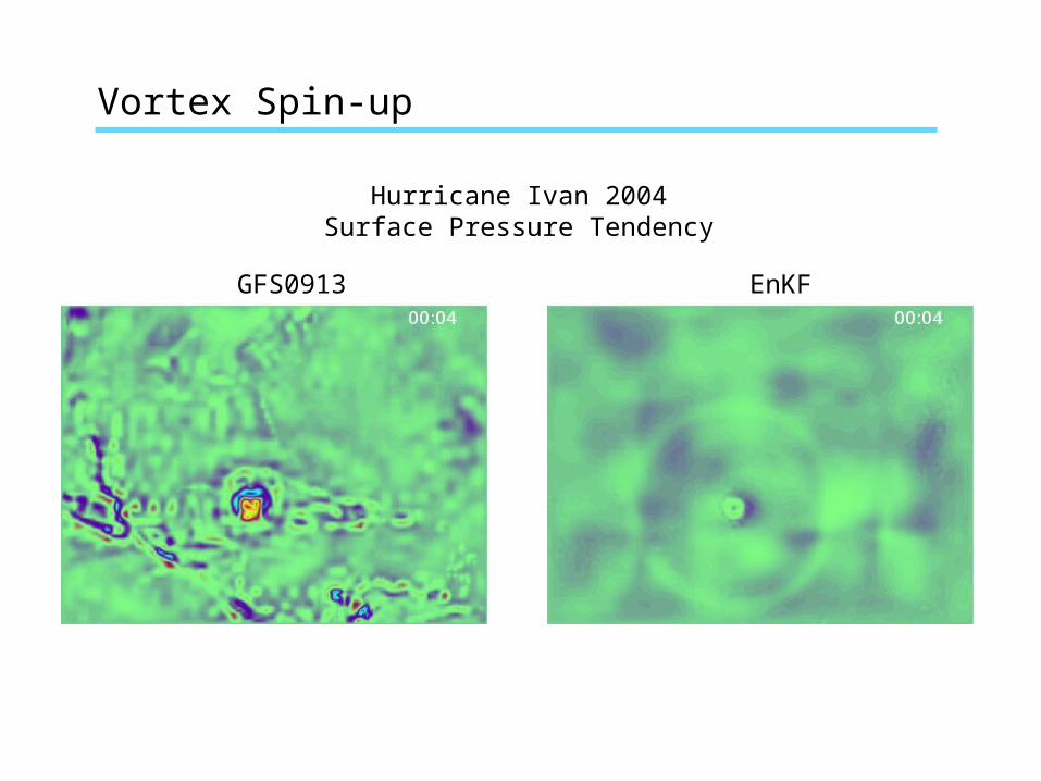
Vortex Spin-up

Hurricane Ivan 2004Surface Pressure Tendency

GFS0913 EnKF

2006 Real-time Forecast

2-way nested domain: 36km (183x133x35) – 12km (103x103x35)

Assimilation window: 12Z – 00Z, every hour

Observations: vortex position, intensity; MADIS satellite wind; dropsondes

Helene (2006)

forecast hour forecast hour

Summary

Hurricane track observations can be easily assimilated with an EnKF---effectiveness depends on frequent, accurate observations.

When position errors are larger, non-Gaussian effects important. General purpose ensemble filters (esp. PF) are not feasible solutions.

Track forecasts initialized from the EnKF analysis are significantly improved in retrospective tests.

EnKF analysis produces dynamically consistent increments, and reduces spurious transient evolution of initial vortex.

EnKF Forecast/Analysis Cycle

1. Forecast: integrate ensemble members to time of next available observations

2. Update members given new observations3. Repeat

EnKF initializes its own ensemble and provides short-range ensemble forecast; unifies DA and

EF

D1

D2D3

.

.obs

obs

WRF/DART for Doppler Radar

Analysis reflectivity (color), obs. (20 dBZ, black contour)

21:10 UTC 21:30 UTC

21:50 UTC 22:10 UTC

km km

kmkm

KOUN

WRF/DART for Doppler Radar

Background minus observation statistics(av’d over 3 analysis cycles/3 elevation angles)

Analysis time (UTC) Analysis time (UTC)

Vel

ocity

(m

/s)

Ref

lect

ivity

(dB

Z)