PUSHOVER_PRESENTACION.pdf
Transcript of PUSHOVER_PRESENTACION.pdf

8/10/2019 PUSHOVER_PRESENTACION.pdf
http://slidepdf.com/reader/full/pushoverpresentacionpdf 1/109

8/10/2019 PUSHOVER_PRESENTACION.pdf
http://slidepdf.com/reader/full/pushoverpresentacionpdf 2/109
The dissertation entitled “The Current Limitations of Displacement Based Design”, by TimothySullivan, has been approved in partial fulfilment of the requirements for the Master Degree in
Earthquake Engineering.
The report is intended to supplement the WG 2 “Displacement Based Design,” commission 7
of fib “seismic design.”
Mervyn Kowalsky ________________________________
Gian Michele Calvi ________________________________
8/10/2019 PUSHOVER_PRESENTACION.pdf
http://slidepdf.com/reader/full/pushoverpresentacionpdf 3/109
Abstract
i
ABSTRACT
Displacement based design methods are emerging as the latest tool for performance based seismicdesign. Of the many different displacement based design procedures proposed in recent years there are
few that are developed to a standard suitable for implementation in modern design codes. Through
application to various case studies this report identifies and discusses the difficulties a designer may
encounter when trying to use displacement based design. It is hoped that by presenting these
limitations efforts will be made to develop the methods further so that designers can begin using the
methods with ease and confidence.
The report incorporates results for five different case studies designed in accordance with eight
different displacement based design methods.
The report focuses on three aspects of the design methods:
1. The relative ease or difficulty with which a design method can be applied and any apparent
limitations a method may have.
2. The required strength obtained for each method and how this compares with the other
methods.
3. The performance of the methods assessed by comparing the predicted ductility or drift values
for each case study with those obtained through time-history analyses.
The case studies indicate that the level of involvement required by the designer does vary considerably
between methods. Some methods are only applicable to certain structural types and others encounter
difficulties with irregular structural forms and flexible foundations. In most instances the designer is
required to make assumptions in order to proceed further and in other instances the method does
simply not facilitate design.

8/10/2019 PUSHOVER_PRESENTACION.pdf
http://slidepdf.com/reader/full/pushoverpresentacionpdf 4/109
Abstract
ii
As a performance based design tool some methods are currently limited to specific earthquake levels
and others do not directly control non-structural damage.
The study proceeds by using each of the design methods to develop design strengths to satisfy a set of
design parameters. Despite all methods using the same set of design parameters, a large variation in
design strength is observed. It is shown that some methods require a design base shear more than five
times that of other methods.
After the designs are complete, non-linear time history analyses are conducted using models with the
strength as obtained for each design. The time-history analyses indicate that all the methods
successfully provide designs that ensure limit states are not exceeded. Despite the large variation in
design strength the variation in drifts observed between methods is relatively low.

8/10/2019 PUSHOVER_PRESENTACION.pdf
http://slidepdf.com/reader/full/pushoverpresentacionpdf 5/109
Acknowledgements
iii
ACKNOWLEDGEMENTS
I thank all members of the Rose School at the University of Pavia, for their friendly assistance
throughout the entire Master course. I also thank North Carolina State University for their supportduring my six week stay in the summer of 2001. I thank my supervisors Mervyn Kowalsky and Gian
Michele Calvi who provided excellent encouragement and guidance. I also thank Nigel Priestley forhis valuable comments and input during preparation of this report. Lastly, I particularly thank my
family in New Zealand and my friends all over the world for their continuing kindness and friendship.

8/10/2019 PUSHOVER_PRESENTACION.pdf
http://slidepdf.com/reader/full/pushoverpresentacionpdf 6/109
Index
iv
THE CURRENT LIMITATIONS OF DISPLACEMENT BASED
DESIGN
INDEX
ABSTRACT
ACKNOWLEDGEMENTS
INDEX
LIST OF TABLES
LIST OF FIGURES
1. INTRODUCTION
1.1 DESIGN CRITERIA
1.2 DESIGN ASSUMPTIONS
2. DESCRIPTION OF THE BUILDINGS CONSIDERED2.1 CASE STUDY 1 – WALL STRUCTURE
2.2 CASE STUDY 2 – WALL STRUCTURE WITH FLEXIBLE FOUNDATION2.3 CASE STUDY 3 –WALL STRUCTURE WITH IRREGULAR LAYOUT
2.4 CASE STUDY 4 – REGULAR RC MOMENT FRAME
2.5 CASE STUDY 5 – VERTICALLY IRREGULAR RC MOMENT FRAME
3. APPLICATION OF THE DESIGN METHODS
3.1 PANAGIOTAKOS AND FARDIS – DEFORMATION CONTROLLED
SEISMIC DESIGN
3.1.1 General Procedure3.1.2 Applied to Case Study 1 – Wall structure
3.1.3 Applied to Case Study 2 – Wall structure with flexible foundation
3.1.4 Applied to Case Study 3 – Wall structure with irregular layout
page
i
iii
iv
viii
ix
1
13
4
4
5
67
8
911
11
12
12
12

8/10/2019 PUSHOVER_PRESENTACION.pdf
http://slidepdf.com/reader/full/pushoverpresentacionpdf 7/109
Index
v
3.1.5 Applied to Case Study 4 – Regular RC Frame Structure3.1.6 Applied to Case Study 5 – Vertically Irregular RC Frame Structure
3.2 BROWNING – PROPORTIONING METHOD FOR RC STRUCTURES
3.2.1 General Procedure3.2.2 Applied to Case Study 4 – Regular RC Frame Structure
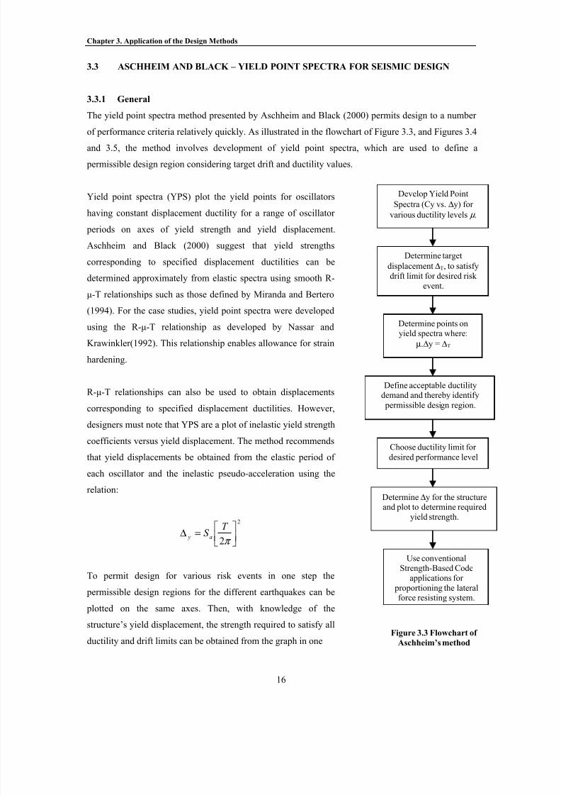
3.3 ASCHHEIM AND BLACK – YIELD POINT SPECTRA FOR SEISMICDESIGN
3.3.1 General
3.3.2 Applied to Case Study 2 – Wall structure with flexible foundation3.3.3 Applied to Case Study 3 – Wall structure with irregular layout
3.3.4 Applied to Case Study 4 – Regular RC Frame Structure
3.3.5 Applied to Case Study 5 – Vertically Irregular RC Frame Structure
3.4 CHOPRA – DBD USING INELASTIC SPECTRA
3.4.1 Applied to Case Study 2 – Wall structure with flexible foundation
3.4.2 Applied to Case Study 3 – Wall structure with irregular layout3.4.3 Applied to Case Study 4 – Regular RC Frame Structure
3.4.4 Applied to Case Study 5 – Vertically Irregular RC Frame Structure
3.5 FREEMAN – CAPACITY SPECTRUM METHOD3.5.1 General
3.5.2 Applied to Case Study 1 – Wall structure3.5.3 Applied to Case Study 2 – Wall structure with flexible foundation
3.5.4 Applied to Case Study 3 – Wall structure with irregular layout
3.5.5 Applied to Case Study 4 – Regular RC Frame Structure
3.5.6 Applied to Case Study 5 – Vertically Irregular RC Frame Structure
3.6 SEAOC – DIRECT DISPLACEMENT BASED DESIGN
3.6.1 General3.6.2 Applied to Case Study 1 – Wall structure
3.6.3 Applied to Case Study 2 – Wall structure with flexible foundation3.6.4 Applied to Case Study 3 – Wall structure with irregular layout
3.6.5 Applied to Case Study 4 – Regular RC Frame Structure
3.6.6 Applied to Case Study 5 – Vertically Irregular RC Frame Structure
3.7 PRIESTLEY AND KOWALSKY – DIRECT DISPLACEMENT BASED
DESIGN3.7.1 General
3.7.2 Applied to Case Study 2 – Wall structure with flexible foundation3.7.3 Applied to Case Study 3 – Wall structure with irregular layout
3.7.4 Applied to Case Study 4 – Regular RC Frame Structure
3.7.5 Applied to Case Study 5 – Vertically Irregular RC Frame Structure
3.8 KAPPOS AND MANAFPOUR – SEISMIC DESIGN WITH ADVANCEDANALYTICAL TECHNIQUES3.8.1 General
3.8.2 Applied to Case Study 3 – Wall structure with irregular layout
3.8.3 Applied to Case Study 4 – Regular RC Frame Structure3.8.4 Applied to Case Study 5 – Vertically Irregular RC Frame Structure
4. REQUIRED STRENGTH COMPARISONS
4.1 FLEXURAL STRENGTH4.1.1 Case Study 1 – Wall structure
1313
14
1415
16
16
1718
19
19
20
2021
21
22
2323
2425
25
25
25
26
2627
2727
27
27
28
28
2929
29
30
31
31
31
3132
33
3434
8/10/2019 PUSHOVER_PRESENTACION.pdf
http://slidepdf.com/reader/full/pushoverpresentacionpdf 8/109

8/10/2019 PUSHOVER_PRESENTACION.pdf
http://slidepdf.com/reader/full/pushoverpresentacionpdf 9/109
Index
vii
6.6 FREEMAN’S METHOD
6.7 THE SEAOC METHOD
6.8 PRIESTLEY’S METHOD
6.8.1 Distribution of strength in proportion to the wall length squared
6.8.2 Use of an assumed displacement profile
6.9 KAPPOS’ METHOD
7 SUMMARY
8 CONCLUSIONS
9 BIBLIOGRAPHY
ANNEX 1. Sample input files for Ruaumoko Time History Analyses
ANNEX 2. Calculations for the case studies (in form of excel spreadsheets on CD)
65
65
65
66
66
67
68
70
72

8/10/2019 PUSHOVER_PRESENTACION.pdf
http://slidepdf.com/reader/full/pushoverpresentacionpdf 10/109
Index
viii
LIST OF TABLES
1.1 SEAOC Recommended Drift Limits associated with Basic Safety Objective 1.2 SEAOC Recommended Displacement Ductility Limits
2.1 Details of the regular moment frame.
3.1 Capacity Design and dynamic magnification recommendations.
4.1 Total Building Design Base Shear for each of the case studies.
4.2 Longitudinal Steel Percentages for Case Study 4 Columns 4.3 Longitudinal Steel Percentages for Case Study 5 Columns
5.1 Design Parameters for the Case Studies
5.2 Governing Design Parameters for Case Study 1 5.3 Drift and Ductility values obtained from Time History Analyses for Case Study 1
5.4 Governing Design Parameters for Case Study 2
5.5 Drift values obtained from Time History Analyses for Case Study 2 5.6 Ductility values obtained from Time History Analyses for Case Study 2
5.7 Governing Design Parameters for Case Study 3 5.8 Drift and Ductility values obtained from Time History Analyses for EQ-I of Case Study 3 5.9 Drift and Ductility values obtained from Time History Analyses for EQ-IV of Case Study 3
5.10 Governing Design Parameters for Case Study 4
5.11 Drift and ductility values obtained from Time History Analyses of Case Study 4 5.12 Governing Design Parameters for Case Study 5
5.13 Drift and ductility values obtained from Time History Analyses of Case Study 5

8/10/2019 PUSHOVER_PRESENTACION.pdf
http://slidepdf.com/reader/full/pushoverpresentacionpdf 11/109

8/10/2019 PUSHOVER_PRESENTACION.pdf
http://slidepdf.com/reader/full/pushoverpresentacionpdf 12/109
Index
x
6.3 Relationship between the structural dimensions, yield displacement and ductility developed considering
the role of initial stiffness used in Chopra’s design method 7.1 Author’s Assessment of the Displacement Based Design Procedures

8/10/2019 PUSHOVER_PRESENTACION.pdf
http://slidepdf.com/reader/full/pushoverpresentacionpdf 13/109
Chapter 1. Introduction
1
1. INTRODUCTION
1.1 DESIGN CRITERIA
The aims of these case studies in displacement based design are threefold:
1. To assess the relative ease or difficulty with which the design methods can be applied and
any apparent limitations the methods may have.
2. To compare the required strength for each method.
3. To consider the performance of the methods by comparing the predicted ductility or drift
values for each case study with those obtained through time-history analysis.
Demand spectra for the case studies are taken from the SEAOC Blue Book (1999). The decision to use
spectra from the SEAOC bluebook is made arbitrarily and does not indicate a limitation of the
methods since any suite of spectra can be used. SEAOC provides displacement response spectra
(DRS), acceleration response spectra (ARS) and acceleration-displacement response spectra (ADRS)
for four different level earthquakes; EQ-I to EQ-IV. For design, the case studies utilise EQ-I,
corresponding to a frequent earthquake and EQ-IV, corresponding to a maximum earthquake. A basic
safety objective is assumed adequate for the building designs and consequently the required building
performance for each earthquake is:
• EQ-I The structural system yield mechanism is partially developed but damage is
generally negligible.
• EQ-IV Damage is major and for structural systems around 80% of the usable
inelastic displacement of the structure is expended. Extensive repairs are required and
may not be economically feasible.
(Refer to Appendix IB-2.3 of SEAOC Blue Book for further details and other levels.)

8/10/2019 PUSHOVER_PRESENTACION.pdf
http://slidepdf.com/reader/full/pushoverpresentacionpdf 14/109
Chapter 1. Introduction
2
70% of the SEAOC EQ-I ground motion has been used for all case studies except Case Study 2 for
which the full EQ-I was used. Details of the case studies are provided in Chapter 2. The decision to
use a reduced EQ-I spectra was made after the design of Case Study 2 showed that the EQ-I event was
controlling the design in all methods. It was considered that the use of a strong EQ-I motion would not
reveal the benefits of effective displacement based design methods. The governing design parameter
for each method is presented with the time-history results for each case study in the performance
assessment of Chapter 5. It is seen that some methods are still controlled by EQ-I even when 70% of
the SEAOC Bluebook demand spectra is used. The PGA values associated with the different spectra
used for design are:
• 70% EQ-I Spectra PGA = 0.11g
• EQ-I Spectra PGA = 0.16g
• EQ-IV Spectra PGA = 0.66g
Design drift limits were also selected from the SEAOC Blue Book. These target values are
shown in Table 1.1 below.
Table 1.1 SEAOC Recommended Drift Limits associated with Basic Safety Objective
System Drift Values related to Earthquake Event
Concrete System EQ-I EQ-II EQ-III EQ-IV
Shear wall H/L=1 0.003 0.0055 0.008 0.010
H/L=2 0.004 0.008 0.012 0.015
H/L=3 0.010 0.019 0.028 0.035
Coupled Shear Wall 0.005 0.015 0.030 0.040
Moment Frame 0.005 0.015 0.030 0.040 For PBSE Design of standard occupancy structures
Some methods require that a system displacement ductility value be maintained. Table 1.2 presents the
SEAOC ductility values selected for use in these case studies. Note that the table does not provide
recommended ductility values for walls with aspect ratio between 5 and 10, nor for values of H/L
greater than 10. SEAOC consider that for high H/L ratio walls, the useful displacement ductility value
of these walls will be limited by the limiting drift ratio.
Table 1.2 SEAOC Recommended Displacement Ductility Limits
System Displacement Ductility Limits for EQ Level
Structural System EQ-I EQ-IV
Shear wall (1 < H/L < 5) 1.0 5.0
Shear wall (H/L = 10) 1.0 2.5
Coupled Shear Wall 1.0 8.0
Moment Resisting Frame 1.0 8.0

8/10/2019 PUSHOVER_PRESENTACION.pdf
http://slidepdf.com/reader/full/pushoverpresentacionpdf 15/109
Chapter 1. Introduction
3
1.2 DESIGN ASSUMPTIONS
Realistic gravity loads are included in the case studies, however, these are only intended for design in
combination with the earthquake loading (with combined loadcase = 1.0G+1.0EQ). The gravity loads
are only used as axial loads for the wall case studies and are applied as uniformly distributed loads
along the beams of the frame case studies. Load cases other than earthquake combined with gravity
are not considered.
Material Properties adopted for design are:
f’c = 27.5 MPa
Ec = 28100 MPa Case Studies 1 & 2 and 32 000 MPa for Case Studies 3, 4 and 5.
f y = 400 MPa
Es = 200 000 MPa
Material strengths are not factored to dependable strength levels for design. Where capacity design is
required an overstrength factor of 1.4 is assumed.
Where a method requires that material strain limits be checked, but does not recommend limiting
values, the following are used:
For EQ-I Concrete compressive strain limit = 0.004
Steel tensile strain limit = 0.015
For EQ-IV Concrete compressive strain limit = 0.018
Steel tensile strain limit = 0.06
Where a method requires values for ultimate curvature for the wall design cases, they are obtained
directly from the expressions developed by Priestley and Kowalsky (1998).
To enable clear comparison between methods the case studies maintain the same dimensions and
member sizes for each design method. Details of the five case studies considered are presented in thefollowing chapter.

8/10/2019 PUSHOVER_PRESENTACION.pdf
http://slidepdf.com/reader/full/pushoverpresentacionpdf 16/109
Chapter 2. Description of the buildings considered
4
2. DESCRIPTION OF THE BUILDINGS CONSIDERED
2.1 CASE STUDY 1 – WALL STRUCTURE
The first case study examines an 8 storey building with walls of equal dimensions in a regular layout
on a rigid foundation. The geometry and layout is shown in Figure 2.1 below.
Figure 2.1 Case Study 1: Wall structure with regular layout on rigid foundation
Earthquake
Six walls of 5m length,250mm in thickness
Neglect contribution of 3
perpendicular walls
(a) Plan view
Earthquake
Six walls of 5m length,250mm in thickness
Neglect contribution of 3
perpendicular walls
(a) Plan view
Storey weight = 5000 kN eachWall axial load ratio = 0.01/storey
8 storeys at 3m each
Rigid foundation beam
(b) Elevation view
Walls respond as linked cantilevers
Storey weight = 5000 kN eachWall axial load ratio = 0.01/storey
8 storeys at 3m each
Rigid foundation beam
(b) Elevation view
Walls respond as linked cantilevers

8/10/2019 PUSHOVER_PRESENTACION.pdf
http://slidepdf.com/reader/full/pushoverpresentacionpdf 17/109
Chapter 2. Description of the buildings considered
5
2.2 CASE STUDY 2 – WALL STRUCTURE WITH FLEXIBLE FOUNDATION
The second case study examines an 8 storey building similar to that of Case Study 1 but with a flexible
foundation. The geometry and layout is shown in Figure 2.2 below.
Figure 2.2 Case Study 2: Wall structure on flexible foundation
Storey weight = 5000 kN each
Wall axial load ratio = 0.01/storey
8 storeys at 3m each
Earthquake
Six walls of 5m length,
250mm in thickness
Neglect contribution of 3
perpendicular walls
Flexible foundation beam
K=5000MNm/rad per wall
(a) Plan view
(b) Elevation view
Walls respond as linked cantilevers
8/10/2019 PUSHOVER_PRESENTACION.pdf
http://slidepdf.com/reader/full/pushoverpresentacionpdf 18/109
Chapter 2. Description of the buildings considered
6
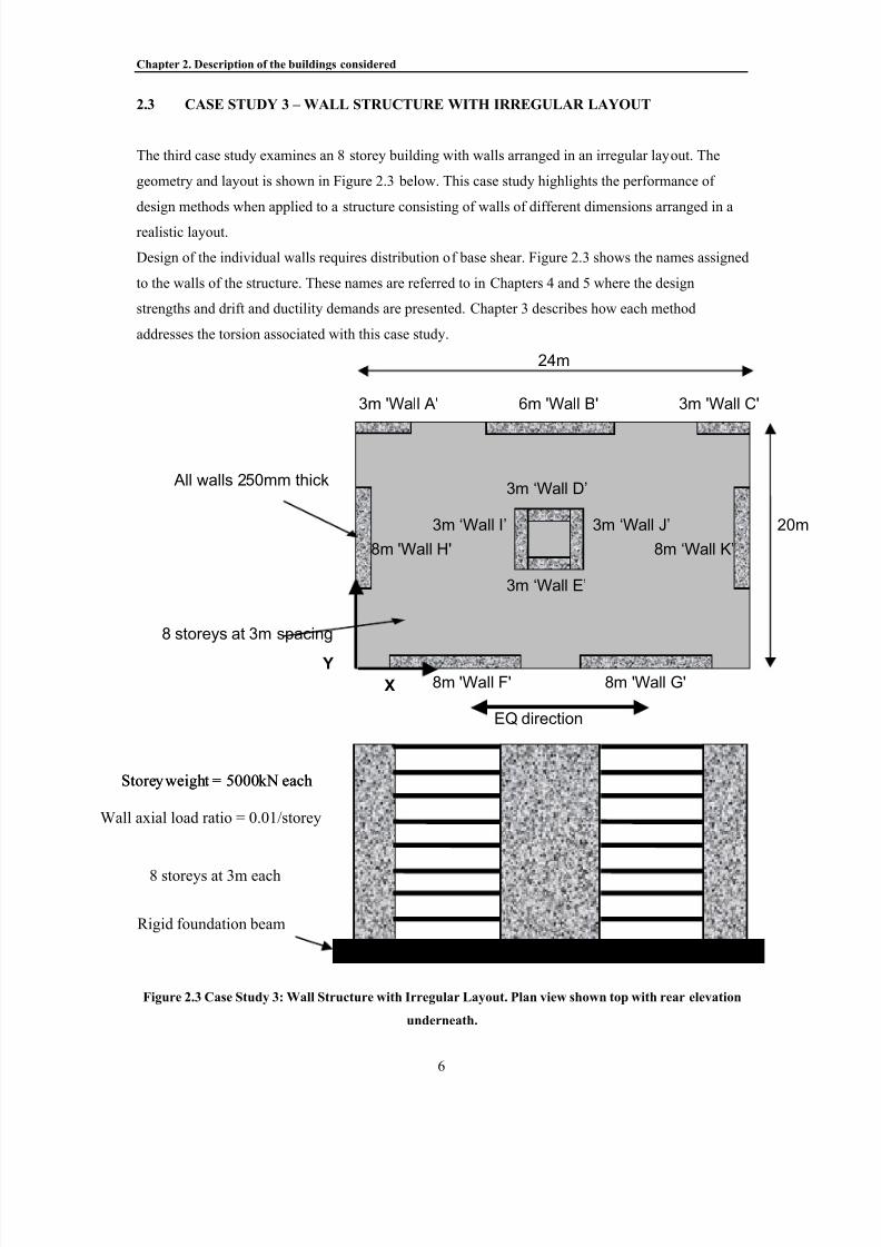
2.3 CASE STUDY 3 – WALL STRUCTURE WITH IRREGULAR LAYOUT
The third case study examines an 8 storey building with walls arranged in an irregular layout. The
geometry and layout is shown in Figure 2.3 below. This case study highlights the performance of
design methods when applied to a structure consisting of walls of different dimensions arranged in a
realistic layout.
Design of the individual walls requires distribution of base shear. Figure 2.3 shows the names assigned
to the walls of the structure. These names are referred to in Chapters 4 and 5 where the design
strengths and drift and ductility demands are presented. Chapter 3 describes how each method
addresses the torsion associated with this case study.
Figure 2.3 Case Study 3: Wall Structure with Irregular Layout. Plan view shown top with rear elevation
underneath.
3m 'Wall A' 6m 'Wall B' 3m 'Wall C'
8 storeys at 3m spacing
24m
20m
All walls 250mm thick
8m 'Wall G'8m 'Wall F'
8m ‘Wall K’8m 'Wall H'
3m ‘Wall D’
3m ‘Wall J’
EQ direction
3m ‘Wall E’
3m ‘Wall I’
X
Y
Storeyweight = 5000 kN each
Wall axial load ratio = 0.01/storey
8 storeys at 3m each
Storeyweight = 5000 kN each
Rigid foundation beam

8/10/2019 PUSHOVER_PRESENTACION.pdf
http://slidepdf.com/reader/full/pushoverpresentacionpdf 19/109

8/10/2019 PUSHOVER_PRESENTACION.pdf
http://slidepdf.com/reader/full/pushoverpresentacionpdf 20/109
Chapter 2. Description of the buildings considered
8
2.5 CASE STUDY 5 – VERTICALLY IRREGULAR RC MOMENT FRAME
The fifth case study examines an 8 storey frame building with a vertically irregular layout. The
geometry is shown in elevation in Figure 2.5 below. This case study considers the performance of
design methods with application to a vertically irregular but realistic structural shape. The building has
a regular layout in plan.
Figure 2.5 Case Study 5: Vertically irregular moment frame
9m 9m 9m9m9m
Beams 650mm deep.
Floors 3000kN each
Beams 800mm deep.
Floors 4000kN each
Beams 900mm deep.
Floors 5000kN each
All columns 800mm deep x
750mm wide.
Rigid foundation
7m
4m
4m
4m
4m
4m
4m
4m
Plan View:
Elevation:

8/10/2019 PUSHOVER_PRESENTACION.pdf
http://slidepdf.com/reader/full/pushoverpresentacionpdf 21/109

8/10/2019 PUSHOVER_PRESENTACION.pdf
http://slidepdf.com/reader/full/pushoverpresentacionpdf 22/109
Chapter 3. Application of the Design Methods
10
SEAOCYes Yes Recommends Paulay Priestley
capacity design procedure.
Priestley
Yes Yes Examples provided show that
capacity design & allowance for
higher modes should be made.
Kappos
No – allows for
strain hardening in
process but not for
material strengths
higher than the
dependable value.
No – inherent in the
time history analysis.
Method factors demand shears by
1.1 to allow for larger EQ than
predicted.
The capacity design procedure described by Paulay and Priestley (1992) is adopted for the case
studies. The effects of the capacity design can be seen directly in the calculations included in the
annex.
Capacity design requirements have little effect on the results of the frame case studies presented in
Chapter 4 because the study chooses to compare only the first floor design beam moments and
reinforcement requirements for the base of the ground storey columns. These members form part of
the desired beam side-sway mechanism and therefore their required flexural strength does not increase
with capacity design. However, the corner base columns were designed assuming that yielding would
occur only after the formation of overstrength of the beams. This assumption results in larger design
axial forces for the columns. The actions that are most affected by capacity design, such as the
member design shear forces and design moments for columns above the first floor are not presented.
During the inelastic time-history analyses the columns above the first floor are modelled elastically
with cracked section properties and the yielding members of the frame are modelled with infinite shear
strength.
For the wall case studies, capacity design magnifies the design shears to allow for overstrength and
dynamic magnification effects. A linear variation of moment resistance is provided from the required
base moment to zero at the top of the building.

8/10/2019 PUSHOVER_PRESENTACION.pdf
http://slidepdf.com/reader/full/pushoverpresentacionpdf 23/109
Chapter 3. Application of the Design Methods
11
3.1 PANAGIOTAKOS AND FARDIS – DEFORMATION CONTROLLED SEISMIC
DESIGN
The design method proposed by Panagiotakos and Fardis (1999) is a deformation calculation based
method using initial stiffnesses with response spectra. The general procedure is illustrated in the
flowchart, Figure 3.1, below.
3.1.1 General procedure
The method allows for checking of a target ductility (equal to 1) for a frequent earthquake (equivalent
to SEAOC EQ-I) and then requires that permissible inelastic rotations are not exceeded for a very rare
earthquake (SEAOC EQ-IV).
Figure 3.1 Flowchart for design procedure of Panagiotakos and Fardis’ method
5. Verify that chord rotation demands areacceptable and modify longitudinal and
transverse steel if necessary.
6. Check and proportion stirrups in joints to
accommodate E -IV ca acit desi n shears.
1. Elastic analysis for non-seismic actions &
“frequent earthquake” (EQ-I) with elastic
spectrum using uncracked sections.
2. Proportioning of steel in hinge locations and
then throughout the structure following the
rules of capacity design for actions from the
elastic anal sis of ste 1.
3. Elastic analysis for “life safety “ (EQ-IV)
earthquake with 5% damped elastic spectrum,
using secant-to-yield member stiffnesses for
antisymmetric bending.
4. Amplification of chord rotations obtained
from elastic analysis of step 3, to estimate
upper characteristic inelastic chord-rotation
demands. The amplification factors are given
in text of the method and were obtained from
extensive time-history analyses.

8/10/2019 PUSHOVER_PRESENTACION.pdf
http://slidepdf.com/reader/full/pushoverpresentacionpdf 24/109
Chapter 3. Application of the Design Methods
12
As a performance based design tool the method could appear restrictive, in the sense that only two
different events can be checked and that non-structural damage (affected by drift) is not controlled. It
is additionally restrictive that design for EQ-IV, the life safety earthquake, requires that either a
serviceability earthquake or ultimate static loads have already been designed for.
3.1.2 Applied to Case Study 1 – Wall structure
The first two steps in the method (as presented in Figure 3.1) are equivalent to force-based design
procedures and did not present any difficulties in application. Step 3 involves the use of secant-to-
yield member stiffnesses for which the method does not provide an expression for wall elements. For
the case studies, the design yield moment Mn and yield curvature φy, were determined and assuming
that bar slippage could be ignored, the effective stiffness EI was calculated as EI = Mn/φy.
Amplification factors required in step 4 of the method are a relatively easy and fast way to obtain
inelastic chord-rotation demands. However, the scaling factors are not provided for wall structures.
For the case study it was assumed that the amplification factors for ground storey columns could be
used.
The method does not recommend expressions for allowable ultimate rotations of wall structures, and
therefore the case study used approximate expressions given by Priestley and Kowalsky (2000).
3.1.3 Applied to Case Study 2 – Wall structure with flexible foundation
The method does not provide advice for designing structures with flexible foundations. It was assumed
that the elastic model used in steps 1 & 3 could simply be modelled with a flexible foundation,
however, it is uncertain whether the same inelastic amplification factors still apply.
3.1.4 Applied to Case Study 3 – Wall structure with irregular layout
No recommendations for the design of wall structures with irregular layout were found and therefore
design proceeded as for Case Study 1. The initial elastic design distributes strength to the walls in
proportion to their length cubed, in accordance with traditional force-based design procedures.

8/10/2019 PUSHOVER_PRESENTACION.pdf
http://slidepdf.com/reader/full/pushoverpresentacionpdf 25/109
Chapter 3. Application of the Design Methods
13
3.1.5 Applied to Case Study 4 – Regular RC Frame Structure
Of all the case studies the method was most easily applied to the frame structures of case studies 4 and
5. This is because the method clearly presents data and equations for the application of the method for
frame structures. Inelastic rotation amplification factors and equations for the secant-to-yield member
stiffness and the allowable ultimate rotation of beams are clearly presented. This is in contrast to wall
structures where several assumptions must be made, as already discussed in Section 3.1.2.
3.1.6 Applied to Case Study 5 – Vertically Irregular RC Frame Structure
No special recommendations for vertically irregular RC frames were found. This did not restrict the
ease in which the method could be applied however, since the same inelastic rotation amplification
factors and design equations as for the regular RC frame were utilised.
Although not examined as a case study in this report, Panagiotakos and Fardis (1999) investigate
frames with infill panels and provide several design recommendations for this irregular structural
form.
8/10/2019 PUSHOVER_PRESENTACION.pdf
http://slidepdf.com/reader/full/pushoverpresentacionpdf 26/109
Chapter 3. Application of the Design Methods
14
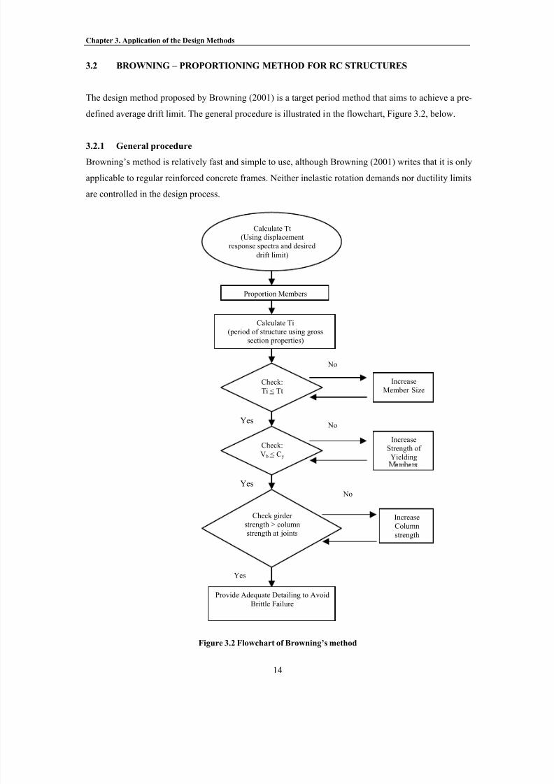
3.2 BROWNING – PROPORTIONING METHOD FOR RC STRUCTURES
The design method proposed by Browning (2001) is a target period method that aims to achieve a pre-
defined average drift limit. The general procedure is illustrated in the flowchart, Figure 3.2, below.
3.2.1 General procedure
Browning’s method is relatively fast and simple to use, although Browning (2001) writes that it is only
applicable to regular reinforced concrete frames. Neither inelastic rotation demands nor ductility limits
are controlled in the design process.
Figure 3.2 Flowchart of Browning’s method
Calculate Tt(Using displacement
response spectra and desired
drift limit)
Proportion Members
Calculate Ti(period of structure using gross
section properties)
Check:
Ti < Tt
Increase
Member Size
No
Yes
Check:
V b < Cy
IncreaseStrength of
Yielding
No
Yes
Check girder
strength > column
strength at joints
Increase
Column
strength
No
Yes
Provide Adequate Detailing to Avoid
Brittle Failure

8/10/2019 PUSHOVER_PRESENTACION.pdf
http://slidepdf.com/reader/full/pushoverpresentacionpdf 27/109
Chapter 3. Application of the Design Methods
15
3.2.2 Applied to Case Study 4 – Regular RC Frame Structure
In determining minimum base shear strength Browning provides an expression that includes an
acceleration factor and a strength reduction factor. It is unclear how sensitive the design would be to
assumptions for the amplification factor, and the case study used the value of 15/4 provided by
Browning for systems with 2% damping.
Consideration was also given to selection of the force reduction factor since many codes use
considerably different factors for identical structural types. For Case Study 4 a force reduction factor
of 8 was used corresponding to the SEAOC allowable ductility value for the appropriate performance
level and structural type considered.
Browning recommends using a structural model with gross section properties and the use of capacity
design and detailing.
The method does not provide advice on how the base shear for the model should be distributed to
determine member actions. It was therefore assumed that it should be proportioned with respect to
mass and height, in line with most modern code approaches.
8/10/2019 PUSHOVER_PRESENTACION.pdf
http://slidepdf.com/reader/full/pushoverpresentacionpdf 28/109
Chapter 3. Application of the Design Methods
16
3.3 ASCHHEIM AND BLACK – YIELD POINT SPECTRA FOR SEISMIC DESIGN
3.3.1 General
The yield point spectra method presented by Aschheim and Black (2000) permits design to a number
of performance criteria relatively quickly. As illustrated in the flowchart of Figure 3.3, and Figures 3.4
and 3.5, the method involves development of yield point spectra, which are used to define a
permissible design region considering target drift and ductility values.
Yield point spectra (YPS) plot the yield points for oscillators
having constant displacement ductility for a range of oscillator
periods on axes of yield strength and yield displacement.
Aschheim and Black (2000) suggest that yield strengths
corresponding to specified displacement ductilities can be
determined approximately from elastic spectra using smooth R-
µ-T relationships such as those defined by Miranda and Bertero
(1994). For the case studies, yield point spectra were developed
using the R-µ-T relationship as developed by Nassar and
Krawinkler(1992). This relationship enables allowance for strain
hardening.
R-µ-T relationships can also be used to obtain displacements
corresponding to specified displacement ductilities. However,
designers must note that YPS are a plot of inelastic yield strength
coefficients versus yield displacement. The method recommends
that yield displacements be obtained from the elastic period of
each oscillator and the inelastic pseudo-acceleration using the
relation:
2
2
=∆
π
T S a y
To permit design for various risk events in one step the
permissible design regions for the different earthquakes can be
plotted on the same axes. Then, with knowledge of the
structure’s yield displacement, the strength required to satisfy all
ductility and drift limits can be obtained from the graph in oneFigure 3.3 Flowchart of
Aschheim’s method
Develop Yield Point
Spectra (Cy vs. ∆y) for
various ductility levels µ .
Determine target
displacement ∆T, to satisfy
drift limit for desired riskevent.
Determine points onyield spectra where:
µ.∆y = ∆T
Define acceptable ductilitydemand and thereby identify
permissible design region.
Determine∆y for the structureand plot to determine required
yield strength.
Use conventionalStrength-Based Code
applications for
proportioning the lateralforce resisting system.
Choose ductility limit for
desired performance level
8/10/2019 PUSHOVER_PRESENTACION.pdf
http://slidepdf.com/reader/full/pushoverpresentacionpdf 29/109

8/10/2019 PUSHOVER_PRESENTACION.pdf
http://slidepdf.com/reader/full/pushoverpresentacionpdf 30/109
Chapter 3. Application of the Design Methods
18
Figure 3.4 Development of Yield Point Spectra (YPS). YPS are developed for the different ductility levels
being considered. The drift control branch of the yield spectrum is formed knowing the equivalent SDOF
system displacement for a given drift limit, and dividing this displacement by the expected ductility.
Figure 3.5 Using the Yield Point Spectra to obtain minimum required strength.
3.3.3 Applied to Case Study 3 – Wall structure with irregular layout
The method does not make recommendations for the design of wall structures with irregular layout. In
accordance with the recommendations provided for regular structures, the required base strength is
Yield Point Spectra for EQ-IV
0.00
0.20
0.40
0.60
0.80
1.00
1.20
0 0.1 0.2 0.3 0.4 0.5
Yield Displacement (m)
Y i e l d S t r e n g t h C o e f f i c i e n t , C
Ductility = 2
Ductility = 4
Ductility = 8
Each yield displacement
multiplied by the ductility
give the peak
displacement.
Peak displacement of
0.40m this case
y∆ y∆2 y∆4
Connection of dots forms
drift control branch
Obtaining Base Shear Coefficient for EQ 1
0.000
0.050
0.100
0.150
0.200
0.250
0.300
0.000 0.050 0.100 0.150 0.200 0.250
Yield displacement (m)
Y i e l d s t r e n g t h c o e f f i c i e n t C
y
Acceptable design
region is above the
branches
Drift control
branch
Ductility control
branch
Enter with
y∆
Obtain
yC

8/10/2019 PUSHOVER_PRESENTACION.pdf
http://slidepdf.com/reader/full/pushoverpresentacionpdf 31/109
Chapter 3. Application of the Design Methods
19
obtained using a system yield displacement and associated system ductility. In an effort to ensure that
individual members of the structure do not undergo excessive ductility demands the yield
displacement of the system is assumed to be that of the longest wall (which has the smallest yield
displacement). The base shear so obtained is proportioned up the height of the structure in relation to
mass and height, and then distributed to the walls in proportion to their length cubed in line with
conventional force based design procedures as recommended by the design method.
3.3.4 Applied to Case Study 4 – Regular RC Frame Structure
The method presents no significant difficulties in application to the Regular RC Frame structure. The
yield displacement is estimated using the yield curvature equations provided by Priestley and
Kowalsky (2000) and assuming that the first floor beam will yield first. In contrast with the Direct
DBD method the design is relatively sensitive to the yield displacement assumed. Because the method
uses the yield displacement to obtain a base shear coefficient directly from demand spectra, as shown
in Figure 3.5, a small difference in yield displacement can result in large difference in design base
shear.
3.3.5 Applied to Case Study 5 – Vertically irregular RC Frame Structure
No special recommendations are made for the design of vertically irregular frame structures. However,
the method presents no significant difficulties in application. The yield displacement is estimated
using the yield curvature equations provided by Priestley and Kowalsky (2000) and assumes that the
first floor beam will yield first.
The method assumes that the structure will respond principally in the first mode. For irregular
structures the mass participation in the first mode and consequently the effective mass and yield
displacement may be significantly different than that of a regular RC frame of similar size. As shown
in Chapter 5, these approximations do not appear to have been too significant for this case study.
However, given that the nature of irregular structures is difficult to predict it may be appropriate to
perform a pushover analysis, as suggested by Aschheim and Black (2000) to obtain a better value for
the yield displacement.

8/10/2019 PUSHOVER_PRESENTACION.pdf
http://slidepdf.com/reader/full/pushoverpresentacionpdf 32/109

8/10/2019 PUSHOVER_PRESENTACION.pdf
http://slidepdf.com/reader/full/pushoverpresentacionpdf 33/109
Chapter 3. Application of the Design Methods
21
3.4.2 Application to Case Study 2 – Wall with flexible foundation
The method provides no recommendations for the design of structures with flexible foundations.
Therefore, in applying the method to Case Study 2 iteration was performed. The system yield
displacement, consisting of the sum of displacements due to the limiting structural deformation and
that due to foundation rotation, was trialled until the resulting design base shear caused the same
system displacement. Due to the inherently iterative nature of Chopra’s method, the requirement for
successive iteration and re-iteration was time consuming.
3.4.3 Applied to Case Study 3 – Wall structure with irregular layout
The method does not make recommendations for the design of wall structures with irregular layout.
Because the method does not recommend how the design base yield strength is proportioned to the
structure it is assumed that strength is distributed in proportion to the wall length cubed, as is the
current practice.
During the iteration process for Case Study 3 it was noted that the method has difficulty iterating on
stiffness for a number of walls. At the end of each iteration the strength is distributed to the walls and
their cracked stiffness is determined as EI = Mn/φy. As these values of stiffness are used to distribute
the base shear at the end of the next iteration it emerges that the shear is distributed totally away from
the smaller walls to be carried entirely by the larger walls. For detailing purposes it was assumed that
minimum steel would then be provided to the smaller walls for which no demand is expected.
3.4.4 Application to Case Study 4 – Regular RC Frame Structure
No recommendations or examples are provided for frame structures. Therefore, to determine the
structural stiffness, cracked section properties were assumed for the beams and the columns. These
values were obtained considering the strength provided and the yield curvature of these members, as
described in Section 3.4.1. As every iteration requires that the design moments be obtained for each
member of the frame, the method is considerably more involved for frame structures versus “single
member” type structures.
One limitation with the current form of the method was observed in designing the frame structure for
the EQ-I level. For this case the code drift limit of 0.5% is less than the predicted yield drift of the
structure. Strictly following the steps of the method (see Figure 3.6) the allowable plastic drift, θP
should then be zero. As the design displacement, ∆D, is equal to: P Y D H θ +∆=∆ , it appears that the
design displacement should therefore equal the yield displacement. If the system displacement
associated with the code drift limit is less than the yield displacement, it becomes apparent that a
design displacement equal to the yield displacement would not prevent the code drift limit being

8/10/2019 PUSHOVER_PRESENTACION.pdf
http://slidepdf.com/reader/full/pushoverpresentacionpdf 34/109
Chapter 3. Application of the Design Methods
22
exceeded. For this report it was assumed that the method intends the target displacement to equal the
lesser of the yield displacement (as explained above) and the displacement associated with the code
drift limit.
If the design displacement is calculated strictly as recommended, the method appears to apply only to
cases where the target drift is less than the yield drift of the structure. This attribute becomes a
limitation if the drift limit is driven by non-structural damage requirements rather than material
inelastic rotation limits as appears to be the situation in Case Study 4.
3.4.5 Applied to Case Study 5 – Vertically Irregular RC Frame Structure
No recommendations are provided for vertically irregular frame structures. Therefore, design
assumptions were similar to those made for the regular frame structure of Case Study 4.
8/10/2019 PUSHOVER_PRESENTACION.pdf
http://slidepdf.com/reader/full/pushoverpresentacionpdf 35/109
Chapter 3. Application of the Design Methods
23
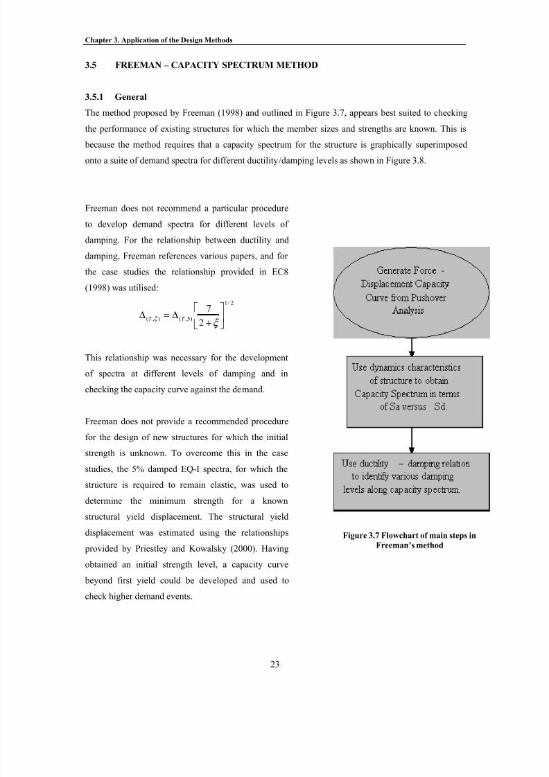
3.5 FREEMAN – CAPACITY SPECTRUM METHOD
3.5.1 General
The method proposed by Freeman (1998) and outlined in Figure 3.7, appears best suited to checking
the performance of existing structures for which the member sizes and strengths are known. This is
because the method requires that a capacity spectrum for the structure is graphically superimposed
onto a suite of demand spectra for different ductility/damping levels as shown in Figure 3.8.
Freeman does not recommend a particular procedure
to develop demand spectra for different levels of
damping. For the relationship between ductility and
damping, Freeman references various papers, and for
the case studies the relationship provided in EC8
(1998) was utilised:
2/1
)5,(),(2
7
+∆=∆
ξ ξ T T
This relationship was necessary for the development
of spectra at different levels of damping and in
checking the capacity curve against the demand.
Freeman does not provide a recommended procedure
for the design of new structures for which the initial
strength is unknown. To overcome this in the case
studies, the 5% damped EQ-I spectra, for which the
structure is required to remain elastic, was used to
determine the minimum strength for a known
structural yield displacement. The structural yield
displacement was estimated using the relationships
provided by Priestley and Kowalsky (2000). Having
obtained an initial strength level, a capacity curve
beyond first yield could be developed and used to
check higher demand events.
Figure 3.7 Flowchart of main steps in
Freeman’s method

8/10/2019 PUSHOVER_PRESENTACION.pdf
http://slidepdf.com/reader/full/pushoverpresentacionpdf 36/109
Chapter 3. Application of the Design Methods
24
Freeman does not prescribe which risk events should be checked nor what an appropriate target
displacement should be. For the case studies, this enabled both the target drift and ductility values to be
considered in determining target displacements. Indeed, the designer can decide what limit states are
important and design for those.
No recommendation is made as to how the base shear should be distributed to the structure, and for the
case studies it was assumed to be with respect to mass and height, in line with most modern codes.
Figure 3.8 Example of the Freeman method - Superimposing a capacity spectrum onto the demand
spectra to check the building performance. In this case the point on the capacity curve with ductility
corresponding to a damping of 20.1% would cross a 20.1% damped demand curve, providing the design
coefficient of approximately 0.2g.
3.5.2 Application to case study 1 – Wall structure
During the design process for Case Study 1 it was found that the strength provided to satisfy EQ-I drift
and ductility criteria, was insufficient for the EQ-IV criteria. The method does not provide
recommendations on how the structure should be improved to satisfy the critical demands of EQ-IV.
For the case study it was assumed that the dimensions would not change and that the strength of the
structure should be increased uniformly. Because increasing the strength does not affect the yield
displacement the new design could simply scale the forces up until the end of the pushover curve
reached the demand curve corresponding to maximum allowable drift or ductility, whichever
governed.
Graphical Solution for Life Safety Earthquake
0
0.2
0.4
0.6
0.8
1
1.2
1.4
1.6
1.8
0.0 0.2 0.4 0.6 0.8 1.0
Spectral Displacement (m)
S p e c t r a l A c c e l e r a t i o n
( g ' s )
5%
10%
20%
12%
14%
16%
20.1%
22.6% at limit
18%
We see that the EQ
generates 0.33m
displacement at20.1% damping and
with Sa = 0.22g

8/10/2019 PUSHOVER_PRESENTACION.pdf
http://slidepdf.com/reader/full/pushoverpresentacionpdf 37/109
Chapter 3. Application of the Design Methods
25
3.5.3 Application to case study 2 – Wall structure with flexible foundation
Freeman does not provide recommendations for structures with flexible foundations. However, it is
assumed in the case studies that by performing a pushover analysis on a model with the appropriate
foundation rotational stiffness the foundation flexibility is adequately accounted for. To obtain the
initial strength, an iterative procedure was followed, whereby a system yield displacement was
guessed and used to obtain a base shear from the elastic response spectra. The moment associated with
this base shear and the consequent foundation rotation were determined and used to evaluate the
system yield displacement.
3.5.4 Application to case study 3 – Wall structure with irregular layout
No recommendations are provided for structures with irregular layout. In addition, for reasons cited in
section 3.5.1 it is uncertain how an initial strength should be assigned to the structure. Therefore, it is
assumed that current force-based procedures are adopted for distribution of strength. Freeman
recommends that a pushover curve is developed to the largest displacement practicable or to the point
where degradation of the overall system occurs. It is assumed that individual wall ductility demands
would be considered in defining the point of overall system degradation.
3.5.5 Applied to Case Study 4 –Regular RC Frame Structure
Several assumptions had to be made for the pushover analysis and development of a model for
pushover analysis is time consuming. The model was developed in Ruaumoko (Carr 2001) with
cracked stiffness of beam elements estimated using Priestley and Kowalsky (2000) yield curvature
equations and the relation EI = Mn/φy. Column interaction diagrams were developed using the Recman
(King et. al. 1986 and Mander et. al. 1988) moment curvature analysis program. The cracked stiffness
was assumed as 50%Ig and 60%Ig for the ground columns and columns above the first floor
respectively. Using the SEAOC drift limit and a factor of 1.4 recommended by Freeman the allowable
roof displacement was related to a displacement at an equivalent SDOF oscillator height. This
displacement was then used to determine the displacement ductility demand, which was compared
with the design value for ductility, and the minimum selected. To compare the pushover curve with the
demand spectra the ductility-damping relation as referenced by Priestley (2001) was utilised.
3.5.6 Applied to Case Study 5 – Vertically irregular RC Frame Structure
Freeman makes no special recommendations for vertically irregular frame structures. Design
incorporated similar assumptions as were made for Case Study 4. The procedure was not complicated
by the irregular nature of the structure.

8/10/2019 PUSHOVER_PRESENTACION.pdf
http://slidepdf.com/reader/full/pushoverpresentacionpdf 38/109
Chapter 3. Application of the Design Methods
26
3.6 SEAOC – DIRECT DISPLACEMENT BASED DESIGN
3.6.1 General
Application of the first of the displacement based design procedures
provided in the SEAOC Blue Book (1999) showed that the procedure
was relatively fast and easy to use to obtain the design base shear.
However, some limitations with the method are noted and several
assumptions had to be made, as detailed below.
As illustrated in Figure 3.9, the method designs for target drift values.
Ductility demands are not controlled. Four different risk events and
drift limits may be considered for design depending on the structural
performance objective.
As part of the design process, the target displacement is used on
spectra at the recommended system damping value. The EC8 (CEN
1996) relationship between damping and ductility was utilised to
convert the target displacement to a value consistent with a 5%
demand spectrum, however, any established relation could be used and
SEAOC make reference to Newmark for this purpose.
For wall structures the method is currently limited to three different
aspect ratios, and does not advise the designer what should be assumed
in the case of a different aspect ratio. For the case studies it was
assumed that interpolation of the data could be performed.
The method recommends that the design base shear be distributed over
the height of the structure with respect to the displaced shape or the
code redistribution with respect to mass and height. No
recommendations are provided for the relative stiffness of members
within the structure. For the case studies it was assumed that commonestimates for cracked section properties (Paulay & Priestley 1992)
should be used for members expected to yield.
Figure 3.9 Flowchart of
SEAOC method

8/10/2019 PUSHOVER_PRESENTACION.pdf
http://slidepdf.com/reader/full/pushoverpresentacionpdf 39/109
Chapter 3. Application of the Design Methods
27
3.6.2 Application to case study 1 – Wall structure
In applying the method to Case Study 1 an inconsistency was noted. The method recommends that the
yield strength of the system be obtained using an overstrength factor divided into the required
effective strength. SEAOC suggests a range of overstrength factors from 1.25 to 2.0, however, it does
not recommend a procedure through which to obtain these factors. With the effective strength known
it was noted that this assumed overstrength factor is likely to predict a yield strength inconsistent with
the yield strength obtained using the ductility demand and the post-yield stiffness ratio. For the case
studies an overstrength value of 1.4 was assumed for the design to EQ-IV and 1.0 for design to EQ-I.
3.6.3 Application to case study 2 – Wall structure with flexible foundations
SEAOC provides no guidance for the design of structures with flexible foundations. Due to the
prescriptive nature of the method it was found that allowance for foundation flexibility could not be
made. This is because the method determines a target displacement using prescribed factors and
assumes a ductility demand. These values are independent of a likely yield displacement or foundation
rotation. If the method had instead calculated the ductility value using yield displacement, and then
determined equivalent damping for this ductility demand, an appropriate effective period could have
been obtained. Despite this restriction in the preliminary design stage it is not likely that non-
conservative designs would be generated since the method would account for negative effects of
foundation flexibility during the pushover analysis.
3.6.4 Applied to Case Study 3 – Wall structure with irregular layout
The method does not make recommendations for the design of wall structures with irregular layouts. It
is assumed that the design distributes the base shear strength to the walls in the proportion to their
length cubed, in accordance with current force-based design practices. No recommendations are
provided for design of structures with walls of different aspect ratio.
3.6.5 Applied to Case Study 4 – Regular RC Frame Structure
The SEAOC method is fast and easy to apply to the regular frame structure of Case Study 4. The base
shear obtained from the design process detailed by SEAOC was then applied to a model of the frame
in SAP2000. The elements of the model had cracked stiffness as recommended by Paulay and
Priestley (1992).
3.6.6 Applied to Case Study 5 – Vertically irregular RC Frame Structure
SEAOC suggests that the effectiveness of the design procedure for irregular structures is likely to be
limited. In application the method presented no more difficulty than the regular frame structure,
however, Chapter 8 shows that the design did not perform very well for this case study.

8/10/2019 PUSHOVER_PRESENTACION.pdf
http://slidepdf.com/reader/full/pushoverpresentacionpdf 40/109
Chapter 3. Application of the Design Methods
28
3.7 PRIESTLEY AND KOWALSKY – DIRECT DISPLACEMENT BASED DESIGN
3.7.1 General
The method proposed by Priestley and Kowalsky (2000) is a relatively fast method that designs a
structure to satisfy a pre-defined drift level. The code drift limit and the drift corresponding to the
system’s inelastic rotation capacity are considered in the design process. The method does not directly
control the system ductility demand.
Figure 3.10 Flowchart of the method by Priestley and Kowalsky
Priestley suggests strain limits for two design states; serviceability and damage control. These two
damage limit states correspond to SEAOC Blue Book performance levels SP1 (EQ-I) and SP4 (EQ-
IV). The designer is able to define appropriate strain limits for design states other than SP1 and SP4
(for example SP2 and SP3).
Determine target
displacement ∆D
using drift limit and assumed
displacement profile.
Determine estimate for system
yield displacement ∆y, and
displacement ductility µ.
Using ξ determine target
displacement ∆D5, equivalent to
SDOF system with 5% damping.
Estimate system damping ξ,
using µ - ξ relationship.
Enter 5% damped DRS with ∆D5
and read off effective period Te.
Use Te & Me to obtain effectivestiffness Ke and thereby the
required base shear
V = Ke∆D
Determine effective mass Me,
Me = ∑mi∆i/∆D
Distribute base shear to structure
in proportion to the assumed
displacement profile.

8/10/2019 PUSHOVER_PRESENTACION.pdf
http://slidepdf.com/reader/full/pushoverpresentacionpdf 41/109
Chapter 3. Application of the Design Methods
29
3.7.2 Application to case study 2 – Wall structure with flexible foundations
The method provides only limited guidance for the design of structures with flexible foundations. The
guidance given recommends calculation of a system damping value that takes into account the
foundation flexibility. Therefore, in application, iteration was used whereby after distribution of
design base shear to the structure, the consequent foundation rotation was determined and used to
evaluate the system yield displacement. This was then used to determine the system ductility demand
and corresponding damping. An effective system period was then determined from which the stiffness
and strength could be obtained (in accordance with the normal procedure - see Figure 3.10. This
process was repeated until system damping values converged.
3.7.3 Applied to Case Study 3 – Wall structure with irregular layout
The method recommends base shear strength is distributed to the walls in the proportion to their length
squared. In development of the design displacement profile it is unclear whether to use the longest
wall, or some average length of all the walls. It was assumed that the longest of the walls should be
used. In accordance with an example presented by Priestley and Kowalsky (2000) for a structure with
varying wall lengths, the equivalent damping of the building was determined using the expected
damping of each wall factored by its length squared over the sum of the squared lengths of the walls. It
was assumed that transverse walls should not be considered in this evaluation of the effective damping
despite the load that they carry due to the twisting of the structure.
3.7.4 Applied to Case Study 4 – Regular RC Frame Structure
The method was relatively easy to apply to the regular frame structure. It was assumed that the yield
displacement would be governed by the yield curvature of the first floor beam. The yield displacement
is used to obtain an estimate for the system damping from the displacement ductility and the base
shear has been shown (Priestley and Kowalsky 2000) to be relatively insensitive to this value of
damping. Hence the method is not very sensitive to the yield displacement. However, in the design of
Case Study 4 for EQ1 an unusual scenario occurred whereby the target drift was less than the yield
drift. Therefore, the required strength was obtained by multiplying the effective stiffness, obtained
from the normal design procedure for a target drift, by the yield displacement. This effectively scales
the design shear up to an appropriate yield strength recognising that the yield drift was larger than the
design target drift. Design actions for individual elements were obtained by modelling the structurewith the predicted effective stiffness of each element and with the base of the ground floor columns
modelled as a pinned connection with the column yield moment applied statically, as described by
Priestley and Kowalsky (2000).

8/10/2019 PUSHOVER_PRESENTACION.pdf
http://slidepdf.com/reader/full/pushoverpresentacionpdf 42/109
Chapter 3. Application of the Design Methods
30
3.7.5 Application to case study 5 – Vertically Irregular Moment Frame.
Integral to Priestley’s method is the assumed displacement profile of the structure at the drift limit.
Displacement profiles have not been developed for irregular structures and therefore the method
cannot strictly be applied to Case Study 5. However, for the purpose of academic interest it was
proposed that the method be applied to Case Study 5 using the displacement profile for a regular
moment frame with number of bays equal to the average of the vertically irregular system. Design
assumptions then followed those as for the regular RC frame structure of Case Study 4.
8/10/2019 PUSHOVER_PRESENTACION.pdf
http://slidepdf.com/reader/full/pushoverpresentacionpdf 43/109
8/10/2019 PUSHOVER_PRESENTACION.pdf
http://slidepdf.com/reader/full/pushoverpresentacionpdf 44/109
Chapter 3. Application of the Design Methods
32
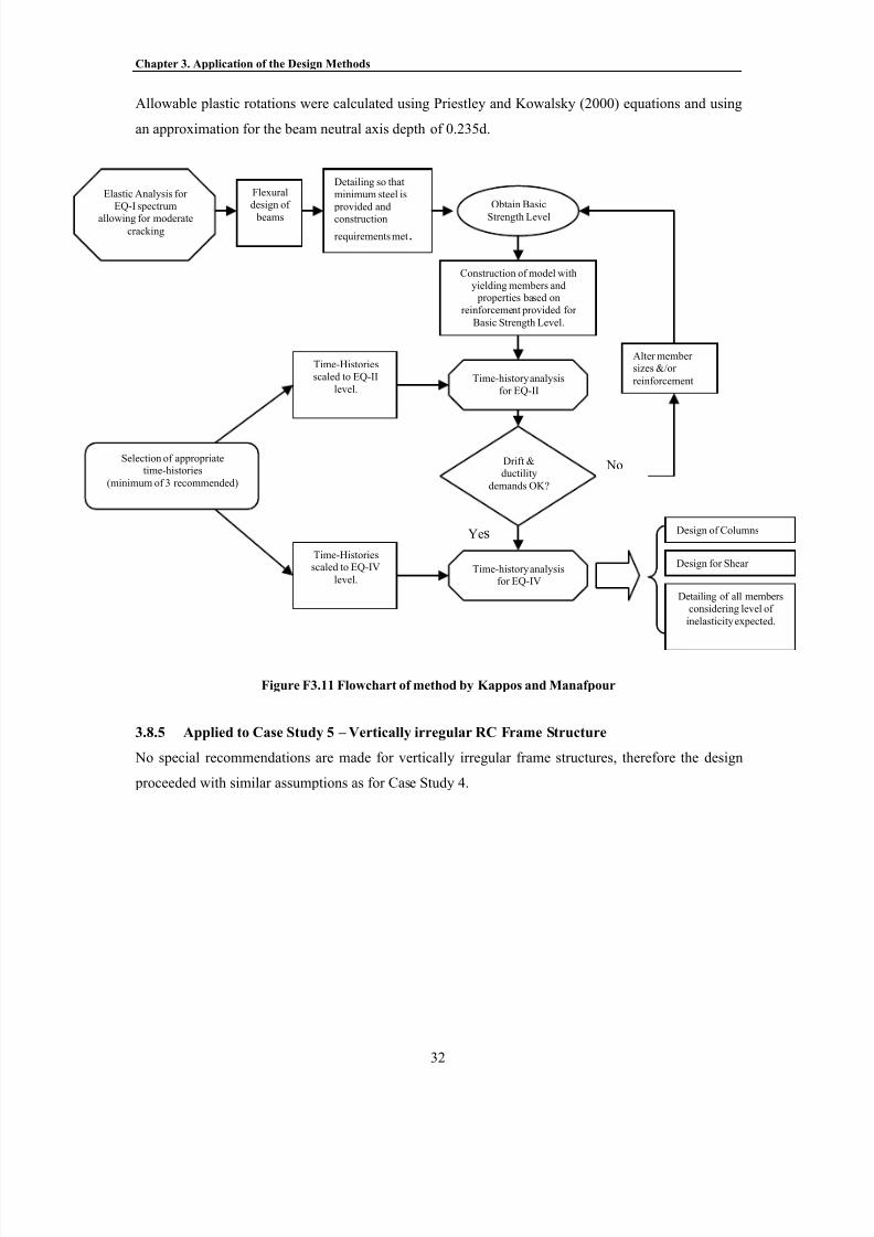
Allowable plastic rotations were calculated using Priestley and Kowalsky (2000) equations and using
an approximation for the beam neutral axis depth of 0.235d.
Figure F3.11 Flowchart of method by Kappos and Manafpour
3.8.5 Applied to Case Study 5 – Vertically irregular RC Frame Structure
No special recommendations are made for vertically irregular frame structures, therefore the design
proceeded with similar assumptions as for Case Study 4.
Detailing so that
minimum steel is
provided and
construction
requirements met.
Obtain Basic
Strength Level
Construction of model with
yielding members and properties based on
reinforcement provided for
Basic Strength Level.
Time-Histories
scaled to EQ-II
level.
Alter membersizes &/or
reinforcement
Drift &ductility
demands OK?
Time-Historiesscaled to EQ-IV
level.
Yes
No
Design of Columns
Design for Shear
Detailing of all members
considering level of
inelasticity expected.
Time-history analysisfor EQ-IV
Time-history analysis
for EQ-II
Elastic Analysis for
EQ-I spectrum
allowing for moderatecracking
Flexural
design of
beams
Selection of appropriatetime-histories
(minimum of 3 recommended)

8/10/2019 PUSHOVER_PRESENTACION.pdf
http://slidepdf.com/reader/full/pushoverpresentacionpdf 45/109
Chapter 4. Required Strength Comparison
33
4 REQUIRED STRENGTH COMPARISONS
The flexural strength, shear strength, and reinforcement content required by each method for each of
the case studies is now presented to illustrate how significant the differences in the methods can be.
Firstly, flexural strength requirements are compared through the use of bending moment diagrams that
allow for capacity design and dynamic magnification as summarised in Chapter 3. Secondly, the
design base shears for the structures at yield are summarised and capacity design shears up the height
of the buildings are also presented. Finally, the flexural reinforcement content for the columns of Case
Studies 4 and 5 are presented.
The performance of each method is assessed by non-linear time history analyses, the results of which
are presented in Chapter 5.
Chapter 6 will identify characteristics of the methods that account for the variation in design actions
presented in this chapter and the likely performance as predicted by the time history analyses of
Chapter 5.

8/10/2019 PUSHOVER_PRESENTACION.pdf
http://slidepdf.com/reader/full/pushoverpresentacionpdf 46/109
Chapter 4. Required Strength Comparison
34
4.1 FLEXURAL STRENGTH
4.1.1 Case Study 1 – Wall structure
Figure 4.1 Design Moments for RC Wall Structure with Rigid Foundation
4.1.2 Case Study 2 – Wall structure with Flexible Foundations
Figure 4.2 Design Moments for RC Wall Structure with Flexible Foundations
Design Moments for a single wall of Case Study 1
RC Wall with Rigid Foundation
01
2
3
4
5
6
7
8
0 5000 10000 15000 20000 25000 30000
Demand Moment (kNm)
L e v e l
Pr - Priestley
S - SEAOC
Pa - Panagiotakos
A - Aschheim
Ch - Chopra
Fr - Freeman
K - Kappos
Pr PaCh
A Fr Se K
Design Moments for a single wall of Case Study 2
RC Wall Structure with Flexible Foundations
0
12
3
4
5
6
7
8
0 5000 10000 15000 20000 25000
Demand Moment (kNm)
L e v e l
Pr - Priestley
S - SEAOC
Pa - Panagiotakos
A - Aschheim
Ch - Chopra
Fr - Freeman
K - Kappos
Pr
PaCh AFr Se K

8/10/2019 PUSHOVER_PRESENTACION.pdf
http://slidepdf.com/reader/full/pushoverpresentacionpdf 47/109
Chapter 4. Required Strength Comparison
35
4.1.3 Case Study 3 – Wall structure with irregular layout
Design bending moments are presented for the 3m ‘Wall A’, the 6m ‘Wall B’ and the 8m ‘Wall F’.
For the location of these walls, refer to Figure 3.3 in Section 3.3.
Figure 4.3 Design Moments for ‘Wall A’ of RC Wall Structure with Irregular Layout
Figure 4.4 Design Moments for ‘Wall B’ of RC Wall Structure with Irregular Layout
Design Bending Moments for 3m 'Wall A' of Case Study 3RC Wall Structure with Irregular Layout
0
1
2
3
4
5
6
7
8
0 2000 4000 6000 8000
Bending Moment (kNm)
L e v e l
Pr - Priestley
S - SEAOC
Pa - Panagiotakos
A - Aschheim
Ch - Chopra
Fr - Freeman
K - Kappos
A PaPr SCh
Fr K
Design Bending Moments for 6m 'Wall B' of Case Study 3
RC Wall Structure with Irregular Layout
0
1
2
3
4
5
6
7
8
0 10000 20000 30000 40000 50000
Bending Moment (kNm)
L e v e l
Pr - Priestley
S - SEAOC
Pa - Panagiotakos
A - Aschheim
Ch - Chopra
Freeman
K - Kappos
A PaPr SCh Fr K

8/10/2019 PUSHOVER_PRESENTACION.pdf
http://slidepdf.com/reader/full/pushoverpresentacionpdf 48/109

8/10/2019 PUSHOVER_PRESENTACION.pdf
http://slidepdf.com/reader/full/pushoverpresentacionpdf 49/109

8/10/2019 PUSHOVER_PRESENTACION.pdf
http://slidepdf.com/reader/full/pushoverpresentacionpdf 50/109
Chapter 4. Required Strength Comparison
38
4.2 SHEAR STRENGTH
Values for the building design base shear strength at yield for each of the methods and all case studies
are shown in Table 4.1 below. The distribution of the capacity design shears up the building height are
presented in sections 4.2.1 to 4.2.5 that follow.
Table 4.1 Total Building Design Base Shear for each of the case studies.
4.2.1 Case Study 1 – Wall structure
Figure 4.8 Capacity Design Shears for Case Study 1 – Wall Structure with Rigid Foundation
Method Case Study 1 Case Study 2 Case Study 3 Case Study 4 Case Study 5
Panagiotakos 9480 7200 10987 13406 7131
Aschheim 3008 5755 4426 3732 4038
Chopra 3416 3750 2434 3077 6307
Freeman 4537 5419 5059 4499 4584SEAOC 4560 4560 3013 3596 3249
Priestley 2900 3494 3417 6136 7623
Kappos 5400 5562 8044 9627 4464
Browning N/A N/A N/A 13369 N/A
Building Design Base Shear
(Base Shear at 1st Yield, kN)
Capacity Design Shears for a single wall from Case Study 1
(Wall Structure with Rigid Foundation)
0
12
3
4
5
6
7
8
0 1000 2000 3000 4000
Capacity Design Shear (kN)
L e v e l
Pr - Priestley
S - SEAOC
Pa - Panagiotakos
A - Aschheim
Ch - Chopra
Fr - Freeman
K - Kappos
Pr PaCh A Fr
SeK

8/10/2019 PUSHOVER_PRESENTACION.pdf
http://slidepdf.com/reader/full/pushoverpresentacionpdf 51/109
Chapter 4. Required Strength Comparison
39
4.2.2 Case Study 2 – Wall structure with Flexible Foundations
Figure 4.9 Capacity Design Shears for Case Study 2 – Wall Structure with Flexible Foundations
4.2.3 Case Study 3 – Wall structure with irregular wall layout
Figure 4.10 Capacity Design Shears for Case Study 3 – Wall Structure with Irregular Layout
Capacity Design Shear for a single wall of Case Study 2
(RC Wall Structure with Flexible Foundations)
0
1
2
3
4
5
6
7
8
0 1000 2000 3000 4000
Capacity Design Shear (kN)
L e v e l
Pr - Priestley
S - SEAOC
Pa - Panagiotakos
A - Aschheim
Ch - Chopra
Fr - Freeman
K - Kappos
Pr PaCh AFr Se K
Capacity Design Shears for Case Study 3
Wall Structure with Irregular Layout
0
1
2
3
4
5
6
7
8
0 5000 10000 15000 20000 25000 30000
Shear (kN)
L e v e l
Pr - Priestley
S - SEAOC
Pa - Panagiotakos
A - Aschheim
Ch - Chopra
F - Freeman
K - Kappos
Pa AS FPr C K
8/10/2019 PUSHOVER_PRESENTACION.pdf
http://slidepdf.com/reader/full/pushoverpresentacionpdf 52/109
Chapter 4. Required Strength Comparison
40
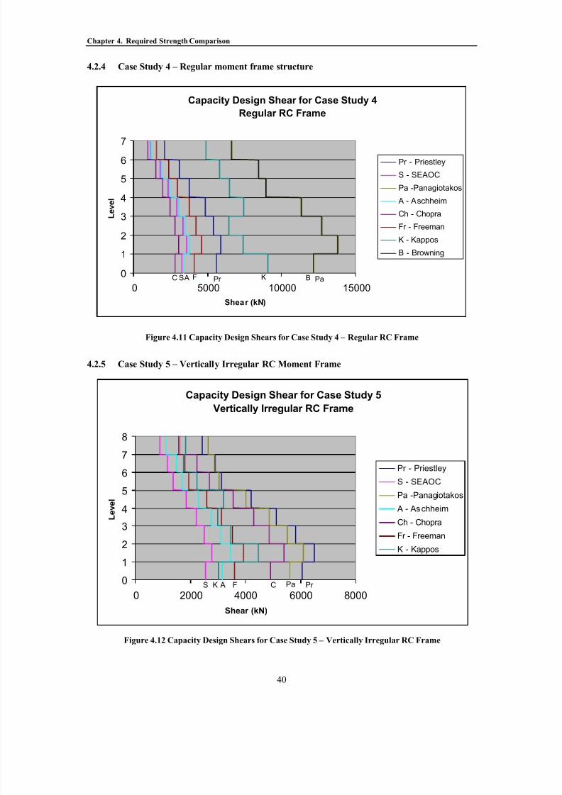
4.2.4 Case Study 4 – Regular moment frame structure
Figure 4.11 Capacity Design Shears for Case Study 4 – Regular RC Frame
4.2.5 Case Study 5 – Vertically Irregular RC Moment Frame
Figure 4.12 Capacity Design Shears for Case Study 5 – Vertically Irregular RC Frame
Capacity Design Shear for Case Study 4
Regular RC Frame
0
1
2
3
4
5
6
7
0 5000 10000 15000
Shear (kN)
L e v e l
Pr - Priestley
S - SEAOC
Pa -Panagiotakos
A - Aschheim
Ch - Chopra
Fr - Freeman
K - Kappos
B - Browning
B PaK AS F Pr C
Capacity Design Shear for Case Study 5
Vertically Irregular RC Frame
0
1
2
3
4
5
6
7
8
0 2000 4000 6000 8000
Shear (kN)
L e v e l
Pr - Priestley
S - SEAOC
Pa -Panagiotakos
A - Aschheim
Ch - Chopra
Fr - Freeman
K - Kappos
PaK AS F Pr C

8/10/2019 PUSHOVER_PRESENTACION.pdf
http://slidepdf.com/reader/full/pushoverpresentacionpdf 53/109
Chapter 4. Required Strength Comparison
41
4.3 RELATIVE STEEL CONTENT AND STEEL DISTRIBUTION
Longitudinal reinforcement ratios are presented for the columns of the frame case studies. These
reinforcement ratios were determined using RECMAN (King et. al. 1986, Mander et. al. 1988)
moment-curvature analyses assuming that the reinforcing steel is distributed evenly to the top, bottom
and sides of the section.
4.3.1 Case Study 4 – Regular RC Moment Frame
Table 4.2 Longitudinal Steel Percentages for Case Study 4 Columns
4.3.2 Case Study 5 – Vertically Irregular RC Moment Frame
Table 4.3 presents the steel contents required by each method for Case Study 5. Some of the steel
contents are excessive and it is expected that in design different column dimensions would be selected.
However, the unrealistic steel contents are presented to highlight the substantial difference in the
strength required for each of the methods.
Table 4.3 Longitudinal Steel Percentages for Case Study 5 Columns
Method
Longitudinal
Steel Interior
Columns
Longitudinal
Steel Corner
Columns
Pana iotakos 1.4% 2.7%
Brownin 1.5% 2.6%
Aschheim 0.3% 0.3%
Cho ra 0.3% 0.3%
Freeman 0.3% 0.4%
SEAOC 0.3% 0.3%
Priestley 0.3% 0.4%
Kappos 0.5% 1.3%
minimum steel assumed = 0.3%
note Pangiotakos already designs columns for ductility reqmnts and
requires 50mm stirrup spacing.
Method
Longitudinal
Steel Interior
Columns
Longitudinal
Steel Corner
Columns
Pana iotakos 6.7% 9.9%
Aschheim 1.0% 1.8%
Chopra 2.3% 3.2%
Freeman 1.5% 2.3%SEAOC 0.8% 1.3%
Priestley 2.6% 3.7%
Ka os 1.3% 2.1%
minimum steel assumed = 0.3%
Assumes no max steel reinforcing content
Also assumes tension steel = side = comp steel

8/10/2019 PUSHOVER_PRESENTACION.pdf
http://slidepdf.com/reader/full/pushoverpresentacionpdf 54/109
8/10/2019 PUSHOVER_PRESENTACION.pdf
http://slidepdf.com/reader/full/pushoverpresentacionpdf 55/109
Chapter 5. Assessment of Performance
43
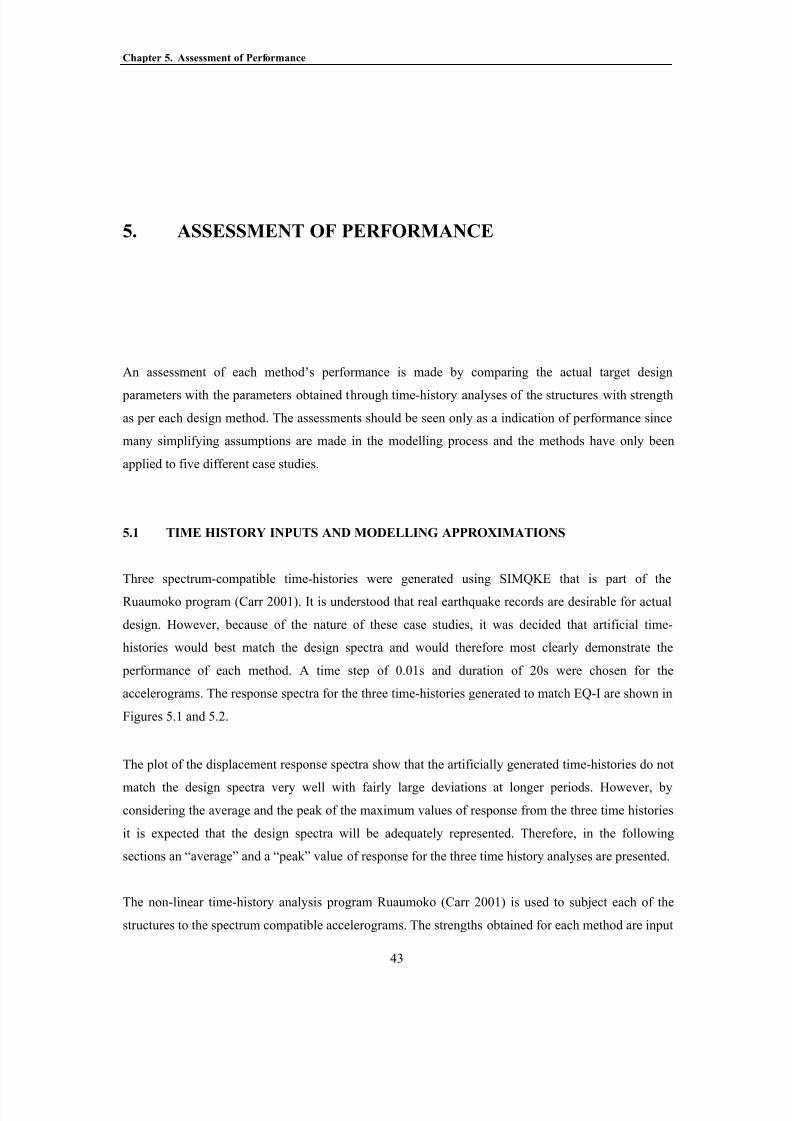
5. ASSESSMENT OF PERFORMANCE
An assessment of each method’s performance is made by comparing the actual target design
parameters with the parameters obtained through time-history analyses of the structures with strength
as per each design method. The assessments should be seen only as a indication of performance since
many simplifying assumptions are made in the modelling process and the methods have only been
applied to five different case studies.
5.1 TIME HISTORY INPUTS AND MODELLING APPROXIMATIONS
Three spectrum-compatible time-histories were generated using SIMQKE that is part of the
Ruaumoko program (Carr 2001). It is understood that real earthquake records are desirable for actual
design. However, because of the nature of these case studies, it was decided that artificial time-
histories would best match the design spectra and would therefore most clearly demonstrate the
performance of each method. A time step of 0.01s and duration of 20s were chosen for the
accelerograms. The response spectra for the three time-histories generated to match EQ-I are shown in
Figures 5.1 and 5.2.
The plot of the displacement response spectra show that the artificially generated time-histories do not
match the design spectra very well with fairly large deviations at longer periods. However, by
considering the average and the peak of the maximum values of response from the three time histories
it is expected that the design spectra will be adequately represented. Therefore, in the following
sections an “average” and a “peak” value of response for the three time history analyses are presented.
The non-linear time-history analysis program Ruaumoko (Carr 2001) is used to subject each of the
structures to the spectrum compatible accelerograms. The strengths obtained for each method are input

8/10/2019 PUSHOVER_PRESENTACION.pdf
http://slidepdf.com/reader/full/pushoverpresentacionpdf 56/109

8/10/2019 PUSHOVER_PRESENTACION.pdf
http://slidepdf.com/reader/full/pushoverpresentacionpdf 57/109
Chapter 5. Assessment of Performance
45
Schonbrich with an unloading stiffness factor of 0.5, reloading stiffness factor of 0.0 and reloading
power factor of 1.0. An explanation of these factors and the shape of the hysteresis model is presented
in the Ruaumoko user manual by Carr (2001).
Elastic damping is modelled for the structures using tangent stiffness Rayleigh damping of
5% applied to the 1st and 2
nd modes. P-delta effects are not considered.
5.1.1 Case Study 1 – Wall Structure
In modelling the wall structure, masses were placed at floor levels assuming the floors to be flexible
out-of-plane, and infinitely stiff in-plane. The strength required for the bottom storey was continued up
the full height of the building and a constant effective stiffness was used over the structure’s height.
5.1.2 Case Study 2 – Wall structure with flexible foundation.
Modelling of the wall structure with the flexible foundation required introduction of a base restraint
with finite rotational stiffness. Note that all the other case studies applied base restraints with infinite
stiffness assuming rigid foundation response.
5.1.3 Case Study 3 – Wall structure with irregular plan and rigid foundation.
Ruaumoko 3D was used to develop a model for the time history analysis of Case Study 3 with
assumptions similar to those of Case Study 1, but with the design strength provided for each level.
Walls perpendicular to the principal earthquake direction are modelled with elastic section properties.
5.1.4 Case study 4 – Regular RC frame structure
A model was developed in Ruaumoko that includes base storey columns with axial load interaction
diagrams, and effective stiffness before yield estimated as 50% Ig using recommendations from Paulay
& Priestley (1992). The columns above the ground floor were modelled as elastic members as yield
should be confined to the base columns and beams by the principles of capacity design. These elastic
columns were modelled with cracked stiffness of 60%Ig, in accordance with Kappos (2001) and
Paulay and Priestley (1992) recommendations.
5.1.5 Case Study 5 – Vertically irregular RC frame structure
A model is used in Ruaumoko making assumptions similar to those of the regular frame model of
Case Study 4.

8/10/2019 PUSHOVER_PRESENTACION.pdf
http://slidepdf.com/reader/full/pushoverpresentacionpdf 58/109
Chapter 5. Assessment of Performance
46
5.2 TIME HISTORY DRIFT AND DUCTILITY VALUES
Peak drift and ductility values are obtained from the time history analyses. They should be compared
with the design parameters as presented in Table 5.1 below. Note that only one parameter will govern
the design of each method. As discussed in Chapter 3, not all parameters are used by all of the
methods.
Table 5.1 Design Parameters for the Case Studies
System Drift Values related to Earthquake Event
Structural System EQ-I Drift EQ-I Ductility EQ-IV Drift EQ-IV Ductility
Shear wall H/L>3 1.0% 1.0 3.5% 5.0
RC Moment Frame 0.5% 1.0 4.0% 8.0
Displacement ductility values are obtained from the analyses by taking the maximum displacement
recorded at an assumed effective height and dividing this by the yield displacement corresponding to
the effective height. For the wall case studies the yield displacement was estimated using the
relationships developed by Priestley and Kowalsky (2000). For the frame case studies the yield
displacement was taken from the pushover analysis performed for the Freeman design. It is noted here
that this yield displacement was shorter than that predicted by the yield displacement equations for
frames developed by Priestley and Kowalsky (2000). This is expected to be because in the Ruaumoko
model the columns above the ground floor are modelled with constant cracked stiffness and the beams
are modelled with a low effective cracked stiffness. The building elastic stiffness and consequently the
yield displacement is dependent on the cracked stiffness assumed for the columns. It is considered that
this scenario whereby the ratio of column and beam stiffness is significantly different than anticipatedoccurs because of inappropriate beam and column dimensions. If shallower beams had been used the
cracked stiffness would have been closer to that assumed when determining the design strengths for
individual elements.
Inter-storey drift values for the wall case studies are the maximum recorded at the top storey as
previous research as discussed by Priestley and Kowalsky (2000) has shown that for wall structures
the peak drift generally occurs at the top floor. For the frame case studies the maximum inter-storey
drift was computed from maximum displacements measured up the height of the building. The use of
the maximum floor displacements is expected to slightly underestimate the maximum inter-storey drift
as it ignores the role of higher mode effects at maximum response. However, it is expected that the
drift values are accurate enough to provide a good indication of the level of drifts developed in the
structure.

8/10/2019 PUSHOVER_PRESENTACION.pdf
http://slidepdf.com/reader/full/pushoverpresentacionpdf 59/109
Chapter 5. Assessment of Performance
47
5.2.1 Case Study 1 – Wall Structure
It is of interest to know which design parameter each method predicted would be critical when
reviewing the drift and ductility values obtained from the time-history analyses. Table 5.2 presents the
parameters that governed the design of Case Study 1 for each method.
Table 5.2 Governing Design Parameters for Case Study 1
The drift and ductility values obtained from time-history analyses presented in Table 5.3 show that all
the methods were successful in maintaining the target design parameters for Case Study 1.
Table 5.3 Drift and Ductility values obtained from Time History Analyses for Case Study 1
5.2.2 Case Study 2 – Wall Structure with Flexible Foundation
When reviewing the drift and ductility values obtained from the time-history analyses it is of interest
to know which design parameter each method predicted would be critical. Table 5.4 presents the
parameters that governed the design of Case Study 2 for each method.
Table 5.4 Governing Design Parameters for Case Study 2
Parameter Governing Design
Panagiotakos EQ-I ductility = 1.0
Aschheim EQ-I ductility = 1.0
Chopra EQ-I code drift = 1.0%
Freeman EQ-IV ductility = 5.0
SEAOC EQ-IV code drift = 3.5%
Priestley EQ-IV inelastic rotation
Kappos EQ-I ductility = 1.0
Method
Peak Average Peak Average Peak Average Peak Average
Panagiotakos 0.47% 0.36% 0.63 0.49 1.6% 1.5% 2.7 2.4
Aschheim 0.75% 0.65% 1.05 0.88 3.1% 2.8% 6.1 5.5
Chopra 0.63% 0.62% 0.83 0.80 2.7% 2.5% 5.3 5.0
Freeman 0.61% 0.49% 0.74 0.63 2.7% 2.4% 5.4 4.6
SEAOC 0.61% 0.49% 0.74 0.63 2.7% 2.4% 5.4 4.6
Priestley 0.76% 0.65% 1.06 0.88 3.0% 2.8% 5.9 5.5Kappos 0.56% 0.45% 0.72 0.60 2.2% 1.9% 3.9 3.4
Note: The 'peak' value refers to the highest maximum value recorded from the three time-history analyses.
The 'average' value refers to the average of the maximum values recorded for each of the three time-history analyses.
time-history top storey
drift
time-history ductility
demand
EQ-I EQ-I EQ-IV EQ-IVtime-history ductility
demand
time-history top storey
drift
Parameter Governing Design
Panagiatakos EQ-I ductility = 1.0
Aschheim EQ-IV structural ductility = 5.0
Chopra EQ-I code drift = 1.0%
Freeman EQ-I ductility = 1.0
SEAOC EQ-IV code drift = 3.5%
Priestley EQ-IV inelastic rotation capacity
Kappos EQ-I ductility = 1.0
Method

8/10/2019 PUSHOVER_PRESENTACION.pdf
http://slidepdf.com/reader/full/pushoverpresentacionpdf 60/109
Chapter 5. Assessment of Performance
48
The drift and ductility values obtained from the time-history analyses presented in Table 5.5 and Table
5.6 show that all the methods were successful in maintaining the target design parameters for Case
Study 2. It is apparent that even though design strengths varied by as much as 100% the maximum
drift values are not significantly different.
Table 5.5 Drift values obtained from Time History Analyses for Case Study 2
Table 5.6 Ductility values obtained from Time History Analyses for Case Study 2
The relatively higher ductility values recorded for the Chopra and Priestley design methods are
somewhat expected since the methods do not attempt to control the displacement ductility and rather
control the inelastic rotation demand to acceptable values.
We also note that even though the SEAOC method only controls the drift and does not allow for
foundation rotation in the design process, the ductility values obtained this case study appear to be
within acceptable levels.
Peak Average Peak Average
Panagiatakos 1.05% 0.74% 2.3% 2.0%
Aschheim 1.02% 0.79% 2.6% 2.4%
Chopra 0.82% 0.76% 3.1% 2.7%
Freeman 0.96% 0.78% 2.7% 2.6%
SEAOC 0.86% 0.74% 2.6% 2.6%
Priestley 1.01% 0.73% 3.1% 2.7%
Kappos 1.03% 0.79% 2.6% 2.4%
The 'peak' value refers to the highest maximum value recorded from the three time-history analyses.The 'average' value refers to the average of the maximum values recorded for each of the three time-history analyses.
EQ-I EQ-IV
top storey drift top storey drift
Peak Average Peak Average Peak Average
Panagiatakos 0.9 0.6 2.0 1.9 3.0 2.7
Aschheim 1.0 0.7 2.7 2.6 3.9 3.7
Chopra 0.8 0.8 4.3 3.8 5.8 5.0Freeman 0.9 0.7 3.3 3.0 4.8 4.3
SEAOC 0.9 0.7 3.2 3.1 4.5 4.3
Priestley 1.1 0.7 4.3 3.8 5.8 5.0
Kappos 1.0 0.7 2.5 2.5 3.7 3.6
The 'peak' value refers to the highest maximum value recorded from the three time-history analyses.
The 'average' value refers to the average of the maximum values recorded for each of the three time-history analyses.
The 'structural ductility' refers to the ductility imposed on the structure accounting for the foundation rotation.
EQ-IV EQ-IVsystem ductility
demand
structural ductility
demand
EQ-Isystem ductility
demand

8/10/2019 PUSHOVER_PRESENTACION.pdf
http://slidepdf.com/reader/full/pushoverpresentacionpdf 61/109
Chapter 5. Assessment of Performance
49
5.2.3 Case Study 3 – Wall Structure with irregular plan and rigid foundation
Table 5.7 presents the parameters that governed the design of Case Study 3 for each method.
Table 5.7 Governing Design Parameters for Case Study 3
The drift and ductility values shown in Figures 5.8 and 5.9 for Case Study 3 were obtained using an
inelastic model in Ruaumoko 3D. The results show that all the methods were successful in maintaining
the target design parameters. However, preliminary analyses for EQ1, obtained using a fibre element
model of the structure, suggested that the methods may underestimate ductility demands on individual
walls of the twisting structure. Although the fibre element model could not be used for the EQ-IV
level due to convergence problems, these observations correspond well with the points made in
Section 6.
The preliminary results disagree with the final results obtained from the Ruaumoko 3D model that
indicate the methods perform satisfactorily for the EQ-I level. This is despite both models having
similar uncracked periods of vibration in both axes of the building. It is felt that the fibre element
model provided a better representation of the cracked section properties at first yield, since actual
material properties were modelled with strain dependent stiffness at all strain levels, in contrast to the
frame element model developed in Ruaumoko that relied on estimates of the cracked stiffness based
on the strength and curvature at first yield.
Table 5.8 Drift and Ductility values obtained from Time History Analyses for EQ-I of Case Study 3
Parameter Governing Design
Panagiatakos EQ-I Ductility Limit = 1.0
Aschheim EQ-I Ductility Limit = 1.0
Chopra EQ-IV 8m Wall Inelastic Rotation
Freeman EQ-IV Ductility Limit = 5.0
SEAOC EQ-IV Drift Limit
Priestley EQ-IV 8m Wall Inelastic Rotation
Kappos EQ-I Ductility Limit = 1.0
Method
Peak Average Peak Average Peak Average Peak Average Peak AveragePanagiatakos 0.34 0.27 0.69 0.54 0.41 0.35 0.45% 0.35% 0.21% 0.18%
Aschheim 0.35 0.33 0.70 0.66 0.58 0.53 0.47% 0.43% 0.30% 0.27%
Chopra 0.35 0.33 0.70 0.66 0.58 0.53 0.46% 0.43% 0.30% 0.27%
Freeman 0.35 0.33 0.70 0.66 0.58 0.53 0.47% 0.43% 0.31% 0.27%
SEAOC 0.35 0.33 0.70 0.66 0.58 0.53 0.46% 0.43% 0.30% 0.27%
Priestley 0.35 0.33 0.70 0.66 0.58 0.53 0.46% 0.43% 0.30% 0.27%
Kappos 0.40 0.30 0.80 0.60 0.53 0.41 0.51% 0.40% 0.28% 0.21%
EQ-I Walls A, B & C EQ-I Walls F & G
Maximum Drift Maximum Drift
EQ-I 3m Wall A EQ-I 6m Wall B EQ-I 8m Wall F
Ductility Demand Ductility Demand Ductility Demand

8/10/2019 PUSHOVER_PRESENTACION.pdf
http://slidepdf.com/reader/full/pushoverpresentacionpdf 62/109
Chapter 5. Assessment of Performance
50
Unfortunately, for many of the design methods minimum steel requirements controlled the strength
and stiffness of the walls. Minimum steel was taken as 0.18% (equal to 0.7/fy as from Paulay &
Priestley [1992]) and the yield curvatures were calculated explicitly for each of the walls with
minimum reinforcement and with known axial load (constant for all methods). Recall that the yield
curvature is used in the calculation of the cracked stiffness and consequently the results of the EQ-I
earthquake analyses are of little interest since the cracked stiffness values (and therefore the elastic
periods) are practically the same for all methods except the Panagiotakos and Kappos methods.
The results for EQ-IV presented in Table 5.9 are of more interest. Keep in mind that this was the
earthquake event that governed most of the methods. Note that the Priestley method receives the
largest average ductility demands, which may be attributed to the base shear distribution procedure,
however, it could also occur due to the irregular nature of the time-histories employed in the analyses.
Table 5.9 Drift and Ductility values obtained from Time History Analyses for EQ-IV of Case Study 3
5.2.4 Case Study 4 – Regular Moment Frame
Table 5.10 presents the parameters that governed the design of Case Study 4 for each method.
Table 5.10 Governing Design Parameters for Case Study 4
The drift and ductility values obtained from time-history analyses presented in Table 5.11 show that
the methods were successful in maintaining the target design parameters for Case Study 4.
Peak Average Peak Average Peak Average Peak Average Peak Average
Panagiatakos 1.48 1.30 2.97 2.60 2.51 1.95 1.72% 1.52% 1.04% 0.84%
Aschheim 1.87 1.71 3.73 3.41 4.34 3.83 2.11% 1.92% 1.90% 1.66%
Chopra 1.97 1.76 3.94 3.53 4.64 4.14 2.20% 2.06% 2.03% 1.89%
Freeman 1.75 1.64 3.50 3.29 4.00 3.64 1.98% 1.85% 1.74% 1.58%
SEAOC 1.97 1.76 3.94 3.53 4.64 4.14 2.20% 2.06% 2.03% 1.89%
Priestley 1.95 1.78 3.90 3.55 4.57 4.15 2.23% 2.06% 2.08% 1.88%
Kappos 1.50 1.38 2.99 2.77 2.57 2.34 1.70% 1.60% 1.09% 1.01%
Ductility Demand Ductility Demand Ductility Demand
EQ-IV Walls F & G
Maximum Drift Maximum Drift
EQ-IV 3m Wall A EQ-IV 6m Wall B EQ-IV 8m Wall F EQ-IV Walls A, B & C
Panagiatakos EQ-I Ductility & EQ-IV inelastic rotation demands
Aschheim EQ-I Drift Limit = 0.5%
Chopra EQ-I Drift Limit = 0.5%
Freeman EQ-I Drift Limit = 0.5%
SEAOC EQ-I Drift Limit = 0.5%
Priestley EQ-I Drift Limit = 0.5%
Kappos EQ-I Ductility Limit = 1.0
Browning EQ-I (threshold strength requirement)
Method Parameter Governing Design

8/10/2019 PUSHOVER_PRESENTACION.pdf
http://slidepdf.com/reader/full/pushoverpresentacionpdf 63/109

8/10/2019 PUSHOVER_PRESENTACION.pdf
http://slidepdf.com/reader/full/pushoverpresentacionpdf 64/109
Chapter 5. Assessment of Performance
52
Table 5.13 Drift and ductility values obtained from Time History Analyses of Case Study 5
5.3 DESIGN DISPLACEMENT VERSUS MAXIMUM RECORDED DISPLACEMENT
To highlight each method’s ability to control displacements the following bar charts compare the
design or “target” displacement with the maximum displacement recorded for the 3 time history
analyses of each case study. Each bar chart compares the displacements at the seismic level that
governed designed as identified in Section 5.2. Therefore, graphs that show a large variation in target
displacement include some methods that were governed by EQ-1 and others that were governed by
EQ-4. The comparison is made of displacements recorded at an assumed effective height, except in the
case of Browning’s method that designs to a roof displacement associated with a drift limit. Where a
method does not directly design for a target displacement, but rather for a certain displacement
ductility limit, then the displacement ductility limit is multiplied by the yield displacement to give the
appropriate target displacement.
It was shown in Section 5.1 that each of the time histories used for the analyses form an envelope
around the design spectra. Therefore, the maximum recorded displacement should be considered as an
upper bound to the peak displacement that would be observed if a time history exactly fitting the
demand spectra were used. The following bar charts show that the maximum recorded displacement
rarely exceeds the design displacement. This is perhaps the clearest means of demonstrating that the
displacement based design methods really do work.
Peak Average Peak Average Peak Average Peak Average
Panagiatakos 0.65% 0.48% 0.62 0.49 3.3% 2.7% 2.5 2.2
Aschheim 0.58% 0.53% 0.54 0.49 3.5% 2.8% 3.7 3.1Chopra 0.64% 0.53% 0.52 0.45 3.1% 2.8% 2.7 2.4
Freeman 0.60% 0.51% 0.58 0.51 3.1% 2.8% 3.2 2.9
SEAOC 0.69% 0.56% 0.62 0.51 3.6% 2.9% 4.1 3.1
Priestley 0.62% 0.46% 0.64 0.49 3.2% 2.9% 2.9 2.4
Kappos 0.64% 0.54% 0.57 0.50 3.1% 2.8% 3.4 3.0
The 'peak' value refers to the highest maximum value recorded from the three time-history analyses.
The 'average' value refers to the average of the maximum values recorded for each of the three time-history analyses.
EQ-IVEQ-I EQ-I EQ-IV
Top storey Drift Ductility DemandTop storey DriftDuctility Demand

8/10/2019 PUSHOVER_PRESENTACION.pdf
http://slidepdf.com/reader/full/pushoverpresentacionpdf 65/109
Chapter 5. Assessment of Performance
53
5.3.1 Displacement Based Design Performance for Case Study 1
Figure 5.3 shows that for Case Study 1 all the methods provide designs that ensure the maximum
displacements are below or not significantly above the target displacement used during design.
0.000 0.100 0.200 0.300 0.400 0.500 0.600
ISDC
YPS
INSPEC
CASPEC
SEAOC
DDBD
T-HIST
Target Displacement (m) Recorded Displacement (m)
Figure 5.3 Comparison of design displacement with maximum recorded displacement for Case Study 1
5.3.2 Displacement Based Design Performance for Case Study 2
Figure 5.4 shows that for Case Study 2 all the methods provide designs that ensure the maximum
displacements are below or not significantly above the target displacement used during design.
0.000 0.100 0.200 0.300 0.400 0.500 0.600 0.700
ISDC
YPS
INSPEC
CASPEC
SEAOC
DDBD
T-HIST
Target Displacement (m) Recorded Displacement (m)
Figure 5.4 Comparison of design displacement with maximum recorded displacement for Case Study 2
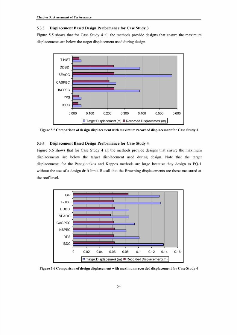
8/10/2019 PUSHOVER_PRESENTACION.pdf
http://slidepdf.com/reader/full/pushoverpresentacionpdf 66/109
Chapter 5. Assessment of Performance
54
5.3.3 Displacement Based Design Performance for Case Study 3
Figure 5.5 shows that for Case Study 4 all the methods provide designs that ensure the maximum
displacements are below the target displacement used during design.
0.000 0.100 0.200 0.300 0.400 0.500 0.600
ISDC
YPS
INSPEC
CASPEC
SEAOC
DDBD
T-HIST
Target Displacement (m) Recorded Displacement (m)
Figure 5.5 Comparison of design displacement with maximum recorded displacement for Case Study 3
5.3.4 Displacement Based Design Performance for Case Study 4
Figure 5.6 shows that for Case Study 4 all the methods provide designs that ensure the maximum
displacements are below the target displacement used during design. Note that the target
displacements for the Panagiotakos and Kappos methods are large because they design to EQ-1
without the use of a design drift limit. Recall that the Browning displacements are those measured at
the roof level.
0 0.02 0.04 0.06 0.08 0.1 0.12 0.14 0.16
ISDC
YPS
INSPEC
CASPEC
SEAOC
DDBD
T-HIST
ISIP
Target Displacement (m) Recorded Displacement (m)
Figure 5.6 Comparison of design displacement with maximum recorded displacement for Case Study 4

8/10/2019 PUSHOVER_PRESENTACION.pdf
http://slidepdf.com/reader/full/pushoverpresentacionpdf 67/109
Chapter 5. Assessment of Performance
55
5.3.5 Displacement Based Design Performance for Case Study 5
Figure 5.7 shows that for Case Study 5 all the methods provide designs that ensure the maximum
displacements are below the target displacement used during design. As was observed for the frame
structure of Case Study 4, the design of Case Study 5 was controlled by EQ-1 for all methods. Note
that the target displacements for the Panagiotakos and Kappos methods are again large because they
design to EQ-1 without the use of a design drift limit.
It has already been noted that the designs of the frame structures for Case Studies 4 and 5 are governed
by an EQ-1 drift limit that is less than the yield drift. This indicates that the drift limits suggested by
SEAOC for frames may be inappropriate, however, if displacement based design methods are to be
used in a performance based design approach it is important that they can design for any target drift,
whether this target drift is less or greater than the yield drift. For instance a performance based design
approach should be able to design a building that has special non-structural drift limit requirements
that may be less than the yield drift.
0 0.05 0.1 0.15 0.2 0.25
ISDC
YPS
INSPEC
CASPEC
SEAOC
DDBD
T-HIST
Target Displacement (m) Recorded Displacement (m)
Figure 5.7 Comparison of design displacement with maximum recorded displacement for Case Study 5
8/10/2019 PUSHOVER_PRESENTACION.pdf
http://slidepdf.com/reader/full/pushoverpresentacionpdf 68/109

8/10/2019 PUSHOVER_PRESENTACION.pdf
http://slidepdf.com/reader/full/pushoverpresentacionpdf 69/109
Chapter 6. Evaluation
57
Figure 6.1 Displacement response spectra showing linear relation between displacement and period
Secondly, consider the equation for the fundamental period of an SDOF oscillator given in 6-2.
K
M T π 2= (6-2)
where, M = Mass
T = Structural period
K = Stiffness
Using the argument, as presented by Priestley and Kowalsky (1998) and Priestley (1998), that stiffness
is proportional to strength, relation 6-3 is written.
V T 1∝ (6-3)
where, V = Strength
Finally, by combining relations 6-1 and 6-3 one obtains equation 6-4 that shows that the displacement
is proportional to the square root of the inverse of the strength.
V S d
1∝ (6-4)
This final relation corresponds with the results observed in these case studies. For instance, consider
the Aschheim and Panagiotakos results for Case Study 1.
The ratio of design strengths between methods is:
15.33008
9480
Asch base
Pan base ==V
V
And the ratio of EQ-1 peak drifts is:
806.1
1
65.0
36.0
Asch
Pan ==δ
δ
Linear relation for
medium length periods
Period, T (s)
Spectral
Displacement
Sd (m)
T1 T2
8/10/2019 PUSHOVER_PRESENTACION.pdf
http://slidepdf.com/reader/full/pushoverpresentacionpdf 70/109
Chapter 6. Evaluation
58
This ratio, as expected is approximately equal to the square root of the inverse of the strength,
2
1
1
2
81.1
1
77.1
1
15.3
1
Disp
Disp
V
V =≈==
In other case studies the displacements were even less dependent on strength than equation 6-4implies. For Case Study 2, the wall structure with flexible foundations, despite ratios of strength
between methods of more than two, the drifts vary by less than 35%.
The foundation flexibility, K fdtn, associated with Case Study 2 effectively reduces the total building
stiffness, K total, below the value of stiffness, K, associated with an equivalent structure having rigid
foundations, as shown in equation 6-5.
fdtntotal K K K
111+= (6-5)
Since a constant value of foundation stiffness is used for all the methods, it is apparent that the
foundation stiffness will act to reduce the ratio of actual stiffness between different methods. For
example, consider two structures that have a structural stiffness equal to 4.0 and 2.0 respectively,
giving a structural stiffness ratio of 2.0. The ratio of total building stiffness for these two structures on
a foundation with a constant stiffness equal to 1.0 is reduced from 2.0 to only 1.2.
The reduction of total stiffness due to foundation flexibility clearly accounts for the reduced influence
strength has on displacements for Case Study 2. However, in Case Studies 4 and 5 drift ratios are also
less than that predicted by relationship 6-4. This could be explained by the large elastic periods of
these structures. As a consequence of long elastic periods the structures do not need to develop large
levels of inelasticity before entering the equal displacement region of the response spectra (seen as the
flat portion of the spectra shown in Figure 6.1). Within the equal displacement region of the spectra
the structures are expected to have the same maximum displacements as is observed for some of the
methods with relatively low design strengths in Case Studies 4 and 5.
6.1.2 Inadequate strength distribution procedures for the EQ1 performance level
For the time-history analyses of Case Study 3 the Ruaumoko 3D model develops drifts and
displacements that indicate the design methods ensure target design parameters are maintained.
However, preliminary results for Case Study 3 obtained using a fibre element model indicated that the
drift and displacement ductility demands for the EQ1 performance level will generally be close to or
above the design limits. This observation is understandable when considering the base shear
distribution procedures adopted by the design methods, all of which do not consider individual wall
yield displacements in relation to the target displacement. All of the methods adopt well established

8/10/2019 PUSHOVER_PRESENTACION.pdf
http://slidepdf.com/reader/full/pushoverpresentacionpdf 71/109
Chapter 6. Evaluation
59
procedures such as those described in Paulay and Priestley (1992) that distribute the design base shear
to each wall in relation to its length cubed (or squared as in the Direct DBD method) with an
adjustment of this shear for torsion effects. To demonstrate why this procedure could be considered
inadequate, Figure 6.2 shows a reasonable target displacement for the EQ1 level in relation to
individual wall yield displacements. The “reasonable” target displacement is selected on the basis that
some ductility demand can be accepted in the critical element of the structure; in this case the 8m wall.
It is of significance that the target displacement is around half the yield displacements of the 3m walls
(Walls A and C from Case Study 3).
Figure 6.2 Possible serviceability target displacement for Case Study 3 in relation to the yield
displacements of the different length walls
We see that by neglecting to consider the yield displacements of the walls in the distribution procedure
the methods are unable to provide a system with sufficient stiffness to develop the design base shear at
the target displacement. The design base shear will instead be developed only when all the walls have
yielded, i.e. at the yield displacement of the smallest wall, in this case the 3m wall.
As the stiffness of the system is lower than intended with the design strength distributed in this
manner, the elastic period and consequently the peak displacement of the structure for the low
intensity earthquake is increased. This has the effect of increasing the displacement ductility demands
on the longest walls, for which yielding is expected before the target displacement is attained. It also
Force
(kN)
y∆ 8m wall y∆ 3m wall Displacement (m)
3m wall stiffness assumed by the
strength distribution procedures
Actual stiffness and therefore the available strength of 3m
wall is less than expected due to large yield displacement
8m WALL
3m WALL
Target displacement
for EQ1 level
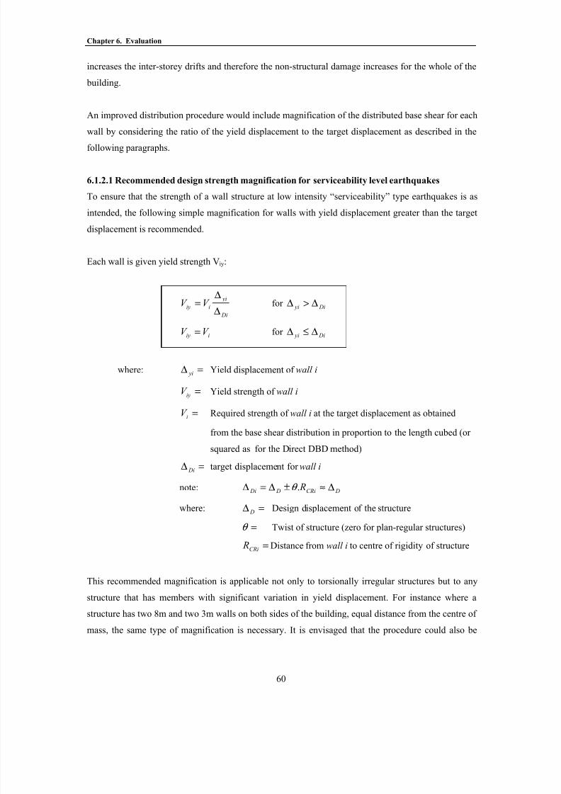
8/10/2019 PUSHOVER_PRESENTACION.pdf
http://slidepdf.com/reader/full/pushoverpresentacionpdf 72/109
Chapter 6. Evaluation
60
increases the inter-storey drifts and therefore the non-structural damage increases for the whole of the
building.
An improved distribution procedure would include magnification of the distributed base shear for each
wall by considering the ratio of the yield displacement to the target displacement as described in the
following paragraphs.
6.1.2.1 Recommended design strength magnification for serviceability level earthquakes
To ensure that the strength of a wall structure at low intensity “serviceability” type earthquakes is as
intended, the following simple magnification for walls with yield displacement greater than the target
displacement is recommended.
Each wall is given yield strength V iy:
Di
yi
iiy V V ∆
∆= for Di yi ∆>∆
iiy V V = for Di yi ∆≤∆
where: =∆ yi Yield displacement of wall i
=iyV Yield strength of wall i
=iV Required strength of wall i at the target displacement as obtained
from the base shear distribution in proportion to the length cubed (or
squared as for the Direct DBD method)
=∆ Di target displacement for wall i
note: DCRi D Di R ∆≈±∆=∆ .θ
where: =∆ D Design displacement of the structure
=θ Twist of structure (zero for plan-regular structures)
=CRi R Distance from wall i to centre of rigidity of structure
This recommended magnification is applicable not only to torsionally irregular structures but to any
structure that has members with significant variation in yield displacement. For instance where a
structure has two 8m and two 3m walls on both sides of the building, equal distance from the centre of
mass, the same type of magnification is necessary. It is envisaged that the procedure could also be

8/10/2019 PUSHOVER_PRESENTACION.pdf
http://slidepdf.com/reader/full/pushoverpresentacionpdf 73/109
Chapter 6. Evaluation
61
extended to hybrid structures which have a combination of frames and walls, provided the yield
displacements for each of the structural elements is known.
6.1.3 Twist induced period lengthening
It is worth pointing out that no recommendations to account for twist-induced period lengthening
were found for any of the methods. This period lengthening occurs in structures such as Case Study 3
because the twist of the structure causes the centre of mass to displace further than the centre of
rigidity. For methods that use a target displacement to obtain the required stiffness, it appears that an
initial estimate of the twist could be used to increase the target displacement. This larger target
displacement would then result in a longer period being designed for. However, neglecting this twist is
unlikely to result in non-conservative design since the structure would essentially be given a shorter
period and higher strength than what is necessary to maintain the target displacement.
Those methods that proceed using the period of the structure implicitly allow for the building twist
lengthening the period of the structure provided that the model used to obtain the period adequately
models the twisting displacement of the mass.
The next part of this chapter discusses points particular to each method that are considered to account
for the variations in performance observed between the methods.
6.2 PANAGIOTAKOS AND FARDIS’ METHOD
Design actions for the method developed by Panagiotakos and Fardis (1999) are generally higher than
the other methods. This is due to the recommendation that an uncracked model of the structure be used
in the initial elastic design to EQ-I. Other methods, including force based design methods, recommend
the use of section properties modified to allow for cracking observed in structures at the point of yield.
An uncracked model is stiffer with shorter periods of vibration than an identical structure with cracked
section properties. Since typical acceleration response spectra are greater at short periods the stiffer
uncracked model attracts a high base shear coefficient. This observation explains why the design
strength for all methods was governed by the initial elastic design to EQ-I.
Panagiotakos and Fardis (1999) discuss the issue of using a cracked model in the presentation of the
method. They suggest that if a ‘serviceability’ earthquake is selected at a level of 30% to 50% of the
‘life safety’ one then internal forces will be about the same as those calculated from force-based
design for the elastic ‘life safety’ earthquake divided by force reduction factor R, or q, of around 5. In
the case studies the ratio between the EQ-IV and EQ-I acceleration response spectra is around 5.75.
Therefore, the high demands obtained for EQ-I are not the result of an unrealistically intense

8/10/2019 PUSHOVER_PRESENTACION.pdf
http://slidepdf.com/reader/full/pushoverpresentacionpdf 74/109
8/10/2019 PUSHOVER_PRESENTACION.pdf
http://slidepdf.com/reader/full/pushoverpresentacionpdf 75/109
Chapter 6. Evaluation
63
6.4 ASCHHEIM’S METHOD
The method presented by Aschheim and Black (2000) is one of two methods examined here that use
inelastic spectra in the design process. It is also one of two methods that utilise ADRS format for
design purposes. The result of this combination is a method that allows design for several limits states
in one step once the spectra have been constructed. The method performs well maintaining the drift
and ductility limits and providing low base shear strength and consequently cost effective design in
relation to other methods.
Integral to the success of the method is a good estimate of yield displacement. In the case studies the
method has benefited from the use of yield displacements obtained using equations for yield curvature
presented by Priestley and Kowalsky (2000). When one considers the shape of the YPS it becomes
apparent that yield displacements more than say 20% from the actual displacement could result in an
increase or decrease in design shear strength by some 50%. Aschheim does suggest that designers can
obtain the yield displacement from pushover analysis, however, this requirement would add significant
time to an otherwise relatively fast design procedure.
6.5 CHOPRA’S METHOD
The method successfully limits the drift demands within the design limits, while providing only a low
level of strength.
The method is not complete as a design tool since it does not provide recommendations for structural
types other than SDOF oscillators, does not recommend a procedure for distribution of shear and does
not suggest procedures for structures with flexible foundations.
Curiously, the method as presented by Chopra (2001), does not detail the principles by which the
method achieves success other than to commend the use of inelastic spectra. During the design process
it was noted that the level of ductility of the SDOF oscillator does not affect the inelastic displacement
spectra at intermediate and long periods. This approximation was shown to be relatively accurate byMiranda and Bertero (2001) through a large number of inelastic time-history analyses. The method
takes advantage of this characteristic behaviour of SDOF oscillators by implicitly suggesting that
initial stiffness therefore governs the displacement response of a system. The system success then
comes from identifying the required initial elastic stiffness required to achieve the target displacement
and multiplying this by a good estimate for yield displacement.

8/10/2019 PUSHOVER_PRESENTACION.pdf
http://slidepdf.com/reader/full/pushoverpresentacionpdf 76/109
Chapter 6. Evaluation
64
Figure 6.3 Relationship between the structural dimensions, yield displacement and ductility developed
considering the role of initial stiffness used in Chopra’s design method
For a structure of given dimensions the yield displacement can be considered constant (Priestley and
Kowalsky 2000). Therefore, for such a structure a unique level of strength will exist that satisfies the
minimum initial stiffness as shown in Figure 6.3. After a designer chooses an acceptable plastic
rotation the target displacement can essentially be fixed and known immediately (an exception occurs
for structures with flexible foundations). Therefore, only one level of strength will satisfy the initial
stiffness that is obtained from the inelastic displacement response spectra.
Keeping the above points in mind, it is also worth noting that Chopra does not recommend a process
for estimation of member sizes. Interestingly, considering that initial elastic stiffness is believed to
control the displacement response, it should be possible to quickly optimise the strength and
proportions of the structure such that the drift limit corresponds to the inelastic rotation limit. For
instance, if structural drift controls the target displacement, dimensions could be increased and a
higher level of ductility developed. Alternatively, if inelastic rotation capacity is controlling, then
dimensions could be reduced and the strength and yield displacement increased. A complication with
this procedure is that the inelastic rotation capacity for larger members is less and as a consequence
even though they can afford lower strength they would need a higher percentage of confinement steel.
Obviously for the smaller walls the reverse is true, in that the percentage of confining steel required
Ductility demand will depend
on the yield displacement of
the structure.
Spectral
Displacement
Spectral
Acceleration
Structures with this initial
elastic stiffness will obtain
same peak displacement, umax.
umaxuy 1 uy 2 uy 3
Yield displacement reduces
with increasing member size.
Unique level of strength
exists for each size
structure to give umax.
8/10/2019 PUSHOVER_PRESENTACION.pdf
http://slidepdf.com/reader/full/pushoverpresentacionpdf 77/109
Chapter 6. Evaluation
65
for inelastic rotation could be reduced even though the longitudinal steel for strength would be
increased.
6.6 FREEMAN’S METHOD
The method developed by Freeman (1998) is intended for the assessment of existing structures. This
project utilised the method for design by using the EQ-I demand spectra to set the initial base shear
strength. Results indicate that the procedure performs well since target design parameters are not
exceeded and the required strength is not excessive. For wall structures with irregular layout it is
important that the pushover analysis identifies the critical elements of the structure rather than
considering the system drift and ductility values. After the assignment of strength initially, pushover
analysis for the EQ-I limit state for irregular structures is likely to improve the performance of the
design procedure. However, this additional task would make the procedure more time consuming.
6.7 THE SEAOC METHOD
The SEAOC (1999) method performs relatively well giving cost efficient design and in general
maintaining the target design parameters. One point where the method may be improved could be
through the identification of an approximate yield displacement for the structure.
Target displacements for the design drift limit could be checked against the yield displacement and the
required effective stiffness adjusted if necessary. It was seen in Case Study 5, where the system yield
drift of 1.0% was twice that of the design drift of 0.5%, that the effective stiffness calculated should
have been multiplied by the yield displacement to obtain the required yield strength. By multiplying
the calculated effective stiffness by the displacement corresponding to the target drift, the effective
stiffness provided was actually equal to half of that intended.
Yield displacement values would also enable the design of structures with flexible foundations since
system ductility and damping values could be calculated relatively quickly. Furthermore, yield
displacements would enable accurate calculation of the required initial stiffness and therefore the
required yield strength for the structure, rather than relying on an estimate for the overstrength factor.
6.8 PRIESTLEY’S METHODThe method developed by Priestley and Kowalsky (2000) performs well giving cost efficient design
while maintaining the target design parameters. Performance appears to be excellent in all case
studies. However as already noted, preliminary time-history analyses for EQ1 of Case Study 3
suggested that for low intensity earthquakes the method may benefit from alternative procedures for
the distribution of strength to walls of differing length.

8/10/2019 PUSHOVER_PRESENTACION.pdf
http://slidepdf.com/reader/full/pushoverpresentacionpdf 78/109
Chapter 6. Evaluation
66
6.8.1 Distribution of strength in proportion to the wall length squared
The initial performance assessment for Case Study 3 suggested that the Direct DBD method develops
higher displacements in relation to other methods. This is not surprising given the points made in
Section 6.1.2 and considering the recommended procedure of distributing the design base shear to the
walls in proportion to their length squared rather than their length cubed as done in the other DBD
methods. While this distribution procedure is most rational (Priestley and Kowalsky 2000) for
structural response where all walls are expected to be yielding, it causes larger displacements and
ductility demands for the frequent EQ-I than other methods with the same total design base shear. By
distributing the design base shear in proportion to the wall length squared, more strength is assigned to
the shorter 3m walls and less to the longer 8m walls in comparison to other design methods. As the
strength of the shorter walls cannot be fully developed at the EQ1 design displacement (refer Section
6.1.2) a smaller percentage of the design base shear can be developed at the design displacement in
comparison to other methods. The structure is consequently provided with much lower elastic stiffness
than anticipated and therefore develops larger displacements and ductility demands than desired.
6.8.2 Use of an assumed displacement profile
Another point regarding the Direct DBD method relates to the use of an assumed displacement profile.
The success of the direct DBD method relies, amongst other things, on the inelastic displacement
profile assumed at the design response. Currently, displacement profiles are provided by Priestley and
Kowalsky (2000) for wall structures assuming that the code drift limit governs design. Indeed, it has
been shown by Kowlasky (2001) that a code drift limit of 2.5% will be critical for the design of walls
with aspect ratio greater than 1. However, the data presented by Kowlasky (2001) also shows that if
the code drift limit is 3.5%, as recommended in the SEAOC Bluebook, then walls of aspect ratio
around 3 to 5 may well be governed by inelastic rotation capacity. Since this inelastic rotation demand
is likely to be developed at the base of a cantilever wall it is assumed that a linear displacement profile
would be utilised. However, a linear profile and perhaps the current displacement profile
recommended for cases where the code drift governs, would not account for higher mode effects that
can be rather significant as shown by the Kappos results presented in Chapter 4.1.1 and 4.1.2.
Despite the dependence of the method on an assumed displacement profile, the method performedwell for the vertically irregular frame structure of Case Study 5. It is noted however, that the design of
Case Study 5 was controlled by the EQ-1 drift limit and it would be interesting to consider the
performance of the method applied to a structure with even greater irregularity that is governed by the
EQ-IV event.

8/10/2019 PUSHOVER_PRESENTACION.pdf
http://slidepdf.com/reader/full/pushoverpresentacionpdf 79/109
Chapter 6. Evaluation
67
6.9 KAPPOS’ METHOD
Design in accordance with Kappos’ method (2001) ensured that the drift and ductility values obtained
from time-history analyses were well within the design limits.
It appears that the design procedure for EQ-I could be made more efficient since throughout the case
studies it was always the strength for EQ-I that governed the design. To improve the design procedure
for EQ-I the method should also take into account the drift limit. The potential benefit of this was seen
in Case Study 5 where the average maximum drift of the structure exceeded the recommended
maximums even though the ductility demand was well within the acceptable value. The method could
combine the drift check it performs for the fairly low intensity EQ-II event. The fact that Kappos
checks the drift for EQ-II but not EQ-I suggests that the method was disadvantaged by the SEAOC
Bluebook EQ-I drift limits that were shown to be less than the yield drift for the frame case studies.
The method could also adopt a check of material strains associated with acceptable damage at the
serviceability limit state rather than a ductility limit of 1.0 as done in other methods.
This method may be considered unnecessarily complex and time consuming for most design situations
since multiple time-history analyses are required. However, the method does provide a thorough
procedure that can be used when the likely inelastic response of a structure appears difficult to predict.

8/10/2019 PUSHOVER_PRESENTACION.pdf
http://slidepdf.com/reader/full/pushoverpresentacionpdf 80/109
Chapter 7. Summary
68
7. SUMMARY
Four properties could be considered valuable to a displacement based design procedure:
• Simplicity – Methods that can be applied relatively quickly and easily are more likely to be
accepted by the design community.
• Versatility – Methods should be able to design a variety of structural forms for a range of
performance levels.
• Performance – Methods should be able to efficiently design a structure to deform to the
extent intended by the target design parameters.
• Completeness – Methods should provide enough information for the designer to be able to
proceed without making too many assumptions. If assumptions are frequently required the
method is prone to misinterpretation.
In applying each of the displacement based design procedures to five different case studies these
qualities have been assessed and are presented in Figure 7.1. Values from 1 to 5 are assigned to each
method for each property where:
• 1 = Very Poor
• 2 = Poor
• 3 = Acceptable
• 4 = Good
• 5 = Excellent
This assessment is obviously subjective and is intended to give the reader a quick impression of how
each method compares.

8/10/2019 PUSHOVER_PRESENTACION.pdf
http://slidepdf.com/reader/full/pushoverpresentacionpdf 81/109
Chapter 7. Summary
69
Figure 7.1 Author’s Assessment of the Displacement Based Design Procedures
Assessment of the Displacement Based Design Methods
0
1
2
3
4
5
P
a n a g i o t a k o
s
B r o w
n i n g
A s c h h e i m
C h o p
r a
F r e e
m a n
S E A O
C
P r i e s t l e y
K a p p o s
SIMPLICITY VERSATILITY PERFORMANCE CLARITY/COMPLETENESS

8/10/2019 PUSHOVER_PRESENTACION.pdf
http://slidepdf.com/reader/full/pushoverpresentacionpdf 82/109
Chapter 8. Conclusions
70
8. CONCLUSIONS
Eight different displacement based design procedures have successfully been applied to 5 different
structural forms. Application has highlighted the strengths and weaknesses of each of the methods. We
see that all the methods successfully maintain the target design parameters even though significant
variation in design strength exists.
It is considered that many of the DBD methods could benefit from the use of alternative target design
parameters that can still ensure accurate performance based design. The different target design
parameters adopted by the methods cause differences in design strengths and yet have relatively little
influence on performance. It would be interesting to compare the strengths obtained by the DBD
methods when they utilise a common target displacement, associated with an agreed set of design
parameters.
The large variation in design strengths between methods has a relatively low influence on peak
displacements due to the relationship between stiffness and displacement. The influence was observed
to reduce with the inclusion of foundation flexibility and where the response entered the equal
displacement range of the spectra.
A new design strength magnification procedure is proposed in Chapter 6 for the performance based
design of structures having walls of different length. The procedure aims to ensure that the stiffness
provided is as intended for design limits associated with seismic events of low intensity.
Limitations have been identified for all of the eight displacement based design methods considered.
These limitations can be considered as minor in some instances and rather major in others. However, it
is also considered that all of these limitations can easily be overcome now that they have been
identified.

8/10/2019 PUSHOVER_PRESENTACION.pdf
http://slidepdf.com/reader/full/pushoverpresentacionpdf 83/109

8/10/2019 PUSHOVER_PRESENTACION.pdf
http://slidepdf.com/reader/full/pushoverpresentacionpdf 84/109
Chapter 9. Bibliography
72
9. BIBLIOGRAPHY
1. Aschheim M.A. and Black E.F. (2000) "Yield Point Spectra for Seismic Design and
Rehabilitation" Earthquake Spectra, Vol. 16, No.2, 317-336.
2. Browning J.P. (2001) "Proportioning of Earthquake-Resistant RC Building Structures" Journal ofthe Structural Division, ASCE , Vol. 127, No.2, 145-151.
3. Carr, A.J. (2001) “Ruaumoko 3D Users Manual” University of Canterbury, Christchurch, NewZealand.
4. Chopra A.K. and Goel R.K. (1999) "Capacity-Demand-Diagram Methods Based on Inelastic
Design Spectrum" Earthquake Spectra, Vol. 15, No.4, 637-656.
5. CEN (1996) European Prestandard ENV 1998: Eurocode 8 – Design provisions for earthquake
resistance of structures. Comite Europeen de Normalisation, Brussels.
6. Chopra A.K. and Goel, R.K. (2001) "Direct Dispalcement-Based Design: Use of Inelastic vs.
Elastic Design Spectra" Earthquake Spectra, Vol. 17, No.1, 47-65.
7. Fajfar P. (2000) "A Nonlinear Analysis Method for Performance-Based Seismic Design"
Earthquake Spectra, Vol. 16, No. 3, 573-592.
8. Fenves (2001) “Structural Dynamics” Course material presented at the ROSE School, theEuropean School of Advanced Studies in Reduction of Seismic Risk, University of Pavia, Italy.
9. Fib TG7.2 (2002), Displacement-based design and assessment, Bulletin in printing.
10. Freeman S.A (1998) "The Capacity Spectrum Method as a Tool for Seismic Design", Proceedings
of the 11th European Conference on Earthquake Engineering, Sept 6-11, Paris.
8/10/2019 PUSHOVER_PRESENTACION.pdf
http://slidepdf.com/reader/full/pushoverpresentacionpdf 85/109
Chapter 9. Bibliography
73
11. Gulkan, P., and Sozen, M. (1974). "Inelastic Response of Reinforced Concrete Structures toEarthquake Motions." ACI Journal , Vol. 71, No.12, 604-610.
12. Kappos A.J. and Manafpour, A. (2001) "Seismic Design of R/C buildings with the Aid of
Advanced Analytical Techniques", Engineering Structures, Vol. 23.
13. King, D.J., Priestley, M.J.N. and Park, R. (1986) “Computer Programs for concrete column
design.” Res. Report 86/12, Department of Civil Engineering, University of Canterbury, New
Zealand.
14. Kowalsky M.J. (2001) “RC Structural Walls Designed According to UBC and Displacement
Based Design Methods” ASCE, Vol. 127, No. 5.
15. Lepage, A. (1997) “A method for drift-control in earthquake-resistant design of reinforced
concrete building structures.” PhD thesis, University of Illinois, Urbana, Illinois.
16. Mander, J.P., Priestley, M.J.N., and Park, R. (1988) “Theoretical stress-strain model for confinedconcrete.” Journal Structural Engineering ASCE, Vol. 114, No.8, 1804-1826.
17. Miranda, E. and Bertero, V.V. (1994). “Evaluation of Strength Reduction Factors for Earthquake-
Resistant Design”, Earthquake Spectra, Vol. 10, No.2.
18. Nassar and Krawinkler (1992) “Seismic design based on ductility and cumulative damage
demands and capacities” Nonlinear Seismic Analysis and Design of Reinforced Concrete Buildings, P. Fajfar and H. Krawinkler, Eds., Elsevier Applied Science, New York.
19. Panagiatakos T.B., Fardis M.N. (1999) "Deformation-Controlled Earthquake-Resistant Design of
RC Buildings" Journal of Earthquake Engineering, Vol. 3 No. 4, 498-518.
20. Paret, T.F, Sasaki, K.K., Eilbekc, D.H., Freeman, S.A. (1996). "Approximate inelastic procedures
to identify failure mechanisms from higher mode effects." 11th World Conference on Earthquake
Engineering , Acapulco, Mexico.
21. Paulay, T. (2000) “Understanding Torsional Phenomena in Ductile Systems” Bulletin of the New
Zealand National Society for Earthquake Engineering , New Zealand National Society forEarthquake Engineering, Silverstream. Vol. 33, No.4.
22. Paulay, T. and Priestley, M.J.N. (1992) “Seismic Design of Concrete and Masonry Buildings.”(John Wiley & Sons Inc. New York) 744 pp.
23. Priestley M.J.N and Calvi, G.M. (1997) “Concepts and procedures for direct displacement-based
design” Seismic Design Methodologies for the Next Generation of Codes, Fajfar and Krawinkler
(eds.), Balkema, Rotterdam, 171-181.

8/10/2019 PUSHOVER_PRESENTACION.pdf
http://slidepdf.com/reader/full/pushoverpresentacionpdf 86/109
Chapter 9. Bibliography
74
24. Priestley M.J.N and Kowalsky M.J. (1998). "Aspects of Drift and Ductility Capacity of CantileverStructural Walls.” Bulletin of the New Zealand National Society for Earthquake Engineering , New
Zealand National Society for Earthquake Engineering, Silverstream. Vol. 31, No.2
25. Priestley M.J.N and Kowalsky M.J. (2000). "Direct Displacement-Based Design of ConcreteBuildings" Bulletin of the New Zealand National Society for Earthquake Engineering , New
Zealand National Society for Earthquake Engineering, Silverstream. Vol. 33, No.4.
26. Priestley M.J.N (1998). "Brief Comments on Elastic Flexibility of Reinforced Concrete Frames,
and Significance to Seismic Design.” Bulletin of the New Zealand National Society for Earthquake Engineering , New Zealand National Society for Earthquake Engineering,
Silverstream. Vol. 31, No.4
27. Priestley M.J.N (2001) “Direct Displacement Based Design Fundamental Considerations”. Part of
course material presented at the ROSE School, the European School of Advanced Studies in
Reduction of Seismic Risk.
28. Qi, X. and Moehle, J.P. (1991) “Displacement design approach for reinforced concrete structures
subjected to earthquakes.” Struct. Res. Series No. 413, Civ. Eng. Studies, University of Illinois,
Urbana, Illinois.
29. SEAOC (1997) Seismic Design Manual. Vol. III (1997 UBC version)
30. SEAOC (1999) Recommended Lateral Force Requirements and Commentary, 7 th Ed.
31. Shibata, A., Sozen, M., (1976). "Substitute Structure Method for Seismic Design in R/C." Journal
of the Structural Division, ASCE , 102(1), 1-18.
32. Shimazaki, K. and Sozen, M.A. (1984). “Seismic drift of reinforced concrete structures.” Tech.Res. Rep. Of Hazama-Gumi, Tokyo, 145-166.

8/10/2019 PUSHOVER_PRESENTACION.pdf
http://slidepdf.com/reader/full/pushoverpresentacionpdf 87/109
ANNEX 1
SAMPLE INPUT FILES FOR THE RUAUMOKO TIME HISTORY ANALYSES

8/10/2019 PUSHOVER_PRESENTACION.pdf
http://slidepdf.com/reader/full/pushoverpresentacionpdf 88/109
RUAUMOKO INPUT FILE: Case Study 1 – Wall Structure with Rigid Foundation
EIGHT STOREY CONCRETE WALL WITH RIGID BASE - Aschheim- all units: kN T & m
2 0 1 0 1 0 0 0 0 0 ! Control Parameters9 8 2 8 1 2 9.81 5.0 5.0 0.01 19.99 1.0 ! Frame and Time-history
10 1 10 3 1 10 1.0 0.1 ! Output and Plotting Options
0 0 ! Iteration Control
NODES
1 0.0 0.0 1 1 1 0 0 0 02 0.0 3.0 0 0 0 0 0 0 0
3 0.0 6.0 0 0 0 0 0 0 0
9 0.0 24.0 0 0 0 0 0 0 0
ELEMENTS
1 1 1 22 2 2 3
3 2 3 4
4 2 4 55 2 5 6
6 2 6 7
7 2 7 88 2 8 9
PROPS1 FRAME
1 0 0 4 0 0 ! Parameters
28.1E6 10.7E6 1.25 0 0.379 0 0 0 0 0 ! Elastic properties with I tangent,
0.0 0.011 1.74 0 ! Bi-linear & Hinge length end 1
0 0 8523 -8523 ! Yield properties0.5 0.0 1.0 2 ! Takeda Parameters
2 FRAME ! Wall sections1 0 0 4 0 0 ! Parameters
28.1E6 10.7E6 1.25 0 0.379 0 0 0 0 0 ! Elastic properties with I tangent
0.0 0.011 1.5 0 ! Bi-linear & Hinge length end 1
0 0 8523 -8523 ! Yield properties0.5 0.0 1.0 2 ! Takeda Parameters
WEIGHT 02 833 0
3 833 0
4 833 0
5 833 06 833 0
7 833 0
8 833 09 833 0
LOADS
2 0.0 -3443 0.0 -344
4 0.0 -344
5 0.0 -3446 0.0 -344
7 0.0 -344
8 0.0 -3449 0.0 -344
EQUAKE
0 1 0.01 1.0

8/10/2019 PUSHOVER_PRESENTACION.pdf
http://slidepdf.com/reader/full/pushoverpresentacionpdf 89/109

8/10/2019 PUSHOVER_PRESENTACION.pdf
http://slidepdf.com/reader/full/pushoverpresentacionpdf 90/109
RUAUMOKO INPUT FILE: Case Study 3 – Wall Structure with Irregular Layout
EIGHT STOREY CONCRETE WALL WITH RIGID BASE - Panagiotakos - all units: kN T & m
2 1 0 0 0 0 0 0 ! Control Parameters108 88 34 8 1 2 9.81 5.0 5.0 0.01 19.99 1.0 ! Wall and Time-history Information
10 1 10 10 1.0 0.1 1.0 0 ! Output and Plotting Options
DEFAULT ! Transformation of Plot axes
0 0 ! Iteration Control
NODES1 0.125 0 -10 1 1 1 1 1 1 0 0
2 1.5 0 -19.875 1 1 1 1 1 1 0 0
3 6 0 -0.125 1 1 1 1 1 1 0 0
4 10.5 0 -10 1 1 1 1 1 1 0 0
5 12 0 -8.5 1 1 1 1 1 1 0 0
6 12 0 -11.5 1 1 1 1 1 1 0 07 12 0 -19.875 1 1 1 1 1 1 0 0
8 13.5 0 -10 1 1 1 1 1 1 0 0
9 18 0 -0.125 1 1 1 1 1 1 0 010 22.5 0 -19.875 1 1 1 1 1 1 0 0
11 23.875 0 -10 1 1 1 1 1 1 0 0
12 0.125 3 -10 2 0 2 0 2 0 101 013 1.5 3 -19.875 2 0 2 0 2 0 101 0
14 6 3 -0.125 2 0 2 0 2 0 101 0
15 10.5 3 -10 2 0 2 0 2 0 101 016 12 3 -8.5 2 0 2 0 2 0 101 0
17 12 3 -11.5 2 0 2 0 2 0 101 0
18 12 3 -19.875 2 0 2 0 2 0 101 0
19 13.5 3 -10 2 0 2 0 2 0 101 0
20 18 3 -0.125 2 0 2 0 2 0 101 021 22.5 3 -19.875 2 0 2 0 2 0 101 0
22 23.875 3 -10 2 0 2 0 2 0 101 0
23 0.125 6 -10 2 0 2 0 2 0 102 024 1.5 6 -19.875 2 0 2 0 2 0 102 0
25 6 6 -0.125 2 0 2 0 2 0 102 0
26 10.5 6 -10 2 0 2 0 2 0 102 0
27 12 6 -8.5 2 0 2 0 2 0 102 028 12 6 -11.5 2 0 2 0 2 0 102 0
29 12 6 -19.875 2 0 2 0 2 0 102 0
30 13.5 6 -10 2 0 2 0 2 0 102 031 18 6 -0.125 2 0 2 0 2 0 102 0
32 22.5 6 -19.875 2 0 2 0 2 0 102 0
33 23.875 6 -10 2 0 2 0 2 0 102 0
34 0.125 9 -10 2 0 2 0 2 0 103 035 1.5 9 -19.875 2 0 2 0 2 0 103 0
36 6 9 -0.125 2 0 2 0 2 0 103 0
37 10.5 9 -10 2 0 2 0 2 0 103 038 12 9 -8.5 2 0 2 0 2 0 103 0
39 12 9 -11.5 2 0 2 0 2 0 103 0
40 12 9 -19.875 2 0 2 0 2 0 103 0
41 13.5 9 -10 2 0 2 0 2 0 103 042 18 9 -0.125 2 0 2 0 2 0 103 0
43 22.5 9 -19.875 2 0 2 0 2 0 103 0
44 23.875 9 -10 2 0 2 0 2 0 103 045 0.125 12 -10 2 0 2 0 2 0 104 0
46 1.5 12 -19.875 2 0 2 0 2 0 104 0
47 6 12 -0.125 2 0 2 0 2 0 104 048 10.5 12 -10 2 0 2 0 2 0 104 0
49 12 12 -8.5 2 0 2 0 2 0 104 050 12 12 -11.5 2 0 2 0 2 0 104 0
51 12 12 -19.875 2 0 2 0 2 0 104 0
52 13.5 12 -10 2 0 2 0 2 0 104 0

8/10/2019 PUSHOVER_PRESENTACION.pdf
http://slidepdf.com/reader/full/pushoverpresentacionpdf 91/109
53 18 12 -0.125 2 0 2 0 2 0 104 054 22.5 12 -19.875 2 0 2 0 2 0 104 0
55 23.875 12 -10 2 0 2 0 2 0 104 0
56 0.125 15 -10 2 0 2 0 2 0 105 057 1.5 15 -19.875 2 0 2 0 2 0 105 0
58 6 15 -0.125 2 0 2 0 2 0 105 0
59 10.5 15 -10 2 0 2 0 2 0 105 0
60 12 15 -8.5 2 0 2 0 2 0 105 061 12 15 -11.5 2 0 2 0 2 0 105 0
62 12 15 -19.875 2 0 2 0 2 0 105 063 13.5 15 -10 2 0 2 0 2 0 105 0
64 18 15 -0.125 2 0 2 0 2 0 105 0
65 22.5 15 -19.875 2 0 2 0 2 0 105 0
66 23.875 15 -10 2 0 2 0 2 0 105 0
67 0.125 18 -10 2 0 2 0 2 0 106 068 1.5 18 -19.875 2 0 2 0 2 0 106 0
69 6 18 -0.125 2 0 2 0 2 0 106 0
70 10.5 18 -10 2 0 2 0 2 0 106 071 12 18 -8.5 2 0 2 0 2 0 106 0
72 12 18 -11.5 2 0 2 0 2 0 106 0
73 12 18 -19.875 2 0 2 0 2 0 106 0
74 13.5 18 -10 2 0 2 0 2 0 106 075 18 18 -0.125 2 0 2 0 2 0 106 0
76 22.5 18 -19.875 2 0 2 0 2 0 106 0
77 23.875 18 -10 2 0 2 0 2 0 106 078 0.125 21 -10 2 0 2 0 2 0 107 0
79 1.5 21 -19.875 2 0 2 0 2 0 107 0
80 6 21 -0.125 2 0 2 0 2 0 107 0
81 10.5 21 -10 2 0 2 0 2 0 107 0
82 12 21 -8.5 2 0 2 0 2 0 107 083 12 21 -11.5 2 0 2 0 2 0 107 0
84 12 21 -19.875 2 0 2 0 2 0 107 085 13.5 21 -10 2 0 2 0 2 0 107 0
86 18 21 -0.125 2 0 2 0 2 0 107 0
87 22.5 21 -19.875 2 0 2 0 2 0 107 0
88 23.875 21 -10 2 0 2 0 2 0 107 0
89 0.125 24 -10 2 0 2 0 2 0 108 090 1.5 24 -19.875 2 0 2 0 2 0 108 0
91 6 24 -0.125 2 0 2 0 2 0 108 0
92 10.5 24 -10 2 0 2 0 2 0 108 093 12 24 -8.5 2 0 2 0 2 0 108 0
94 12 24 -11.5 2 0 2 0 2 0 108 0
95 12 24 -19.875 2 0 2 0 2 0 108 0
96 13.5 24 -10 2 0 2 0 2 0 108 097 18 24 -0.125 2 0 2 0 2 0 108 0
98 22.5 24 -19.875 2 0 2 0 2 0 108 0
99 23.875 24 -10 2 0 2 0 2 0 108 0100 12 0 -10 1 1 1 1 1 1 0 0
101 12 3 -10 0 1 0 1 0 1 0 0
102 12 6 -10 0 1 0 1 0 1 0 0
103 12 9 -10 0 1 0 1 0 1 0 0104 12 12 -10 0 1 0 1 0 1 0 0105 12 15 -10 0 1 0 1 0 1 0 0
106 12 18 -10 0 1 0 1 0 1 0 0
107 12 21 -10 0 1 0 1 0 1 0 0108 12 24 -10 0 1 0 1 0 1 0 0
ELEMENTS1 1 1 12 0 0 X 0
2 3 2 13 0 0 Z 0
3 6 3 14 0 0 Z 04 2 4 15 0 0 X 0
8/10/2019 PUSHOVER_PRESENTACION.pdf
http://slidepdf.com/reader/full/pushoverpresentacionpdf 92/109
5 5 5 16 0 0 Z 06 5 6 17 0 0 Z 0
7 4 7 18 0 0 Z 0
8 2 8 19 0 0 X 09 6 9 20 0 0 Z 0
10 3 10 21 0 0 Z 0
11 1 11 22 0 0 X 0
12 1 12 23 0 0 X 013 7 13 24 0 0 Z 0
14 10 14 25 0 0 Z 015 2 15 26 0 0 X 0
16 9 16 27 0 0 Z 0
17 9 17 28 0 0 Z 0
18 8 18 29 0 0 Z 0
19 2 19 30 0 0 X 020 10 20 31 0 0 Z 0
21 7 21 32 0 0 Z 0
22 1 22 33 0 0 X 023 1 23 34 0 0 X 0
24 11 24 35 0 0 Z 0
25 14 25 36 0 0 Z 0
26 2 26 37 0 0 X 027 13 27 38 0 0 Z 0
28 13 28 39 0 0 Z 0
29 12 29 40 0 0 Z 030 2 30 41 0 0 X 0
31 14 31 42 0 0 Z 0
32 11 32 43 0 0 Z 0
33 1 33 44 0 0 X 0
34 1 34 45 0 0 X 035 15 35 46 0 0 Z 0
36 18 36 47 0 0 Z 037 2 37 48 0 0 X 0
38 17 38 49 0 0 Z 0
39 17 39 50 0 0 Z 0
40 16 40 51 0 0 Z 0
41 2 41 52 0 0 X 042 18 42 53 0 0 Z 0
43 15 43 54 0 0 Z 0
44 1 44 55 0 0 X 045 1 45 56 0 0 X 0
46 19 46 57 0 0 Z 0
47 22 47 58 0 0 Z 0
48 2 48 59 0 0 X 049 21 49 60 0 0 Z 0
50 21 50 61 0 0 Z 0
51 20 51 62 0 0 Z 052 2 52 63 0 0 X 0
53 22 53 64 0 0 Z 0
54 19 54 65 0 0 Z 0
55 1 55 66 0 0 X 056 1 56 67 0 0 X 057 23 57 68 0 0 Z 0
58 26 58 69 0 0 Z 0
59 2 59 70 0 0 X 060 25 60 71 0 0 Z 0
61 25 61 72 0 0 Z 0
62 24 62 73 0 0 Z 063 2 63 74 0 0 X 0
64 26 64 75 0 0 Z 0
65 23 65 76 0 0 Z 066 1 66 77 0 0 X 0

8/10/2019 PUSHOVER_PRESENTACION.pdf
http://slidepdf.com/reader/full/pushoverpresentacionpdf 93/109
67 1 67 78 0 0 X 068 27 68 79 0 0 Z 0
69 30 69 80 0 0 Z 0
70 2 70 81 0 0 X 071 29 71 82 0 0 Z 0
72 29 72 83 0 0 Z 0
73 28 73 84 0 0 Z 0
74 2 74 85 0 0 X 075 30 75 86 0 0 Z 0
76 27 76 87 0 0 Z 077 1 77 88 0 0 X 0
78 1 78 89 0 0 X 0
79 31 79 90 0 0 Z 0
80 34 80 91 0 0 Z 0
81 2 81 92 0 0 X 082 33 82 93 0 0 Z 0
83 33 83 94 0 0 Z 0
84 32 84 95 0 0 Z 085 2 85 96 0 0 X 0
86 34 86 97 0 0 Z 0
87 31 87 98 0 0 Z 0
88 1 88 99 0 0 X 0
PROPS
1 FRAME1 0 0 0 0 0 0 ! Wall H & K Floor 1
3.20E+07 1.28E+07 2 0 3.841 3.841 1.67 1.67 0 0 0 ! E G A Jxx Izz Iyy Asz Asy Sy Sz Wgt
0 0 0 0 0 0 10 10 ! Section end properties
2 FRAME1 0 0 0 0 0 0 ! Wall I & J Floor 1
3.20E+07 1.28E+07 0.75 0 0.224 0.224 0.625 0.625 0 0 0 ! E G A Jxx Izz Iyy Asz Asy Sy Sz Wgt0 0 0 0 0 0 10 10 ! Section end properties
3 FRAME
1 0 0 0 4 0 0 ! Wall A & C Floor 1
3.20E+07 1.28E+07 0.75 0 0.116 0.116 0.625 0.625 0 0 0 ! E G A Jxx Izz Iyy Asz Asy Sy Sz Wgt0 0 0 0 0 0 10 10 ! Section end properties
0.99 0.99 0.05 0.05 ! Bi-linear factors
1.61 0 0 0 ! Hinge lengths end 10 0 0 0 0 0 ! Axial and Torsion Yield
2863 -2863 2863 -2863 ! Yield properties
0.5 0.0 1.0 2 !Takeda Properties
4 FRAME
1 0 0 0 4 0 0 ! Wall B Floor 1
3.20E+07 12816000 1.5 0 1.096 1.0959 1.25 1.25 0 0 0 ! E G A Jxx Izz Iyy Asz Asy Sy Sz Wgt0 0 0 0 0 0 10 10 ! Section end properties
0.99 0.99 0.05 0.05 ! Bi-linear factors
1.94 0 0 0 ! Hinge lengths end 1
0 0 0 0 0 0 ! Axial and Torsion Yield18694 -18694 18694 -18694 ! Yield properties0.5 0.0 1.0 2.0 !Takeda Properties
5 FRAME1 0 0 0 4 0 0 ! Wall D & E Floor 1
32041000 12816000 0.75 0 0.165 0.1654 0.625 0.625 0 0 0 ! E G A Jxx Izz Iyy Asz Asy Sy Sz Wgt
0 0 0 0 0 0 10 10 ! Section end properties0.99 0.99 0.05 0.05 ! Bi-linear factors
1.61 0 0 0 ! Hinge lengths end 1
0 0 0 0 0 0 ! Axial and Torsion Yield4671 -4671 4671 -4671 ! Yield properties

8/10/2019 PUSHOVER_PRESENTACION.pdf
http://slidepdf.com/reader/full/pushoverpresentacionpdf 94/109

8/10/2019 PUSHOVER_PRESENTACION.pdf
http://slidepdf.com/reader/full/pushoverpresentacionpdf 95/109
56 765.4 0 765.457 187.5 0 187.5
58 453.0 0 453.0
59 390.5 0 390.560 390.5 0 390.5
61 390.5 0 390.5
62 531.1 0 531.1
63 390.5 0 390.564 453.0 0 453.0
65 187.5 0 187.566 765.4 0 765.4
67 765.4 0 765.4
68 187.5 0 187.5
69 453.0 0 453.0
70 390.5 0 390.571 390.5 0 390.5
72 390.5 0 390.5
73 531.1 0 531.174 390.5 0 390.5
75 453.0 0 453.0
76 187.5 0 187.5
77 765.4 0 765.478 765.4 0 765.4
79 187.5 0 187.5
80 453.0 0 453.081 390.5 0 390.5
82 390.5 0 390.5
83 390.5 0 390.5
84 531.1 0 531.1
85 390.5 0 390.586 453.0 0 453.0
87 187.5 0 187.588 765.4 0 765.4
89 765.4 0 765.4
90 187.5 0 187.5
91 453.0 0 453.0
92 390.5 0 390.593 390.5 0 390.5
94 390.5 0 390.5
95 531.1 0 531.196 390.5 0 390.5
97 453.0 0 453.0
98 187.5 0 187.5
99 765.4 0 765.4
LOADS
EQUAKE
0 1 0.01 1.0

8/10/2019 PUSHOVER_PRESENTACION.pdf
http://slidepdf.com/reader/full/pushoverpresentacionpdf 96/109
8/10/2019 PUSHOVER_PRESENTACION.pdf
http://slidepdf.com/reader/full/pushoverpresentacionpdf 97/109
54 8.5852 26.215 0 0 055 9.7028 4.267 0 0 0
56 9.7028 7.925 0 0 0
57 9.7028 11.583 0 0 058 9.7028 15.241 0 0 0
59 9.7028 18.899 0 0 0
60 9.7028 22.557 0 0 0
61 9.7028 26.215 0 0 062 17.7292 4.267 0 0 0
63 17.7292 7.925 0 0 064 17.7292 11.583 0 0 0
65 17.7292 15.241 0 0 0
66 17.7292 18.899 0 0 0
67 17.7292 22.557 0 0 0
68 17.7292 26.215 0 0 069 18.8468 4.267 0 0 0
70 18.8468 7.925 0 0 0
71 18.8468 11.583 0 0 072 18.8468 15.241 0 0 0
73 18.8468 18.899 0 0 0
74 18.8468 22.557 0 0 0
75 18.8468 26.215 0 0 076 26.8732 4.267 0 0 0
77 26.8732 7.925 0 0 0
78 26.8732 11.583 0 0 079 26.8732 15.241 0 0 0
80 26.8732 18.899 0 0 0
81 26.8732 22.557 0 0 0
82 26.8732 26.215 0 0 0
83 27.9908 4.267 0 0 084 27.9908 7.925 0 0 0
85 27.9908 11.583 0 0 086 27.9908 15.241 0 0 0
87 27.9908 18.899 0 0 0
88 27.9908 22.557 0 0 0
89 27.9908 26.215 0 0 0
90 36.0172 4.267 0 0 091 36.0172 7.925 0 0 0
92 36.0172 11.583 0 0 0
93 36.0172 15.241 0 0 094 36.0172 18.899 0 0 0
95 36.0172 22.557 0 0 0
96 36.0172 26.215 0 0 0
ELEMENTS
1 1 1 2
2 3 2 37 3 7 8
8 2 9 10
9 4 10 11
14 4 15 1615 2 17 1816 4 18 19
21 4 23 24
22 2 25 2623 4 26 27
28 4 31 32
29 1 33 3430 3 34 35
35 3 39 40
36 6 2 4137 8 3 42

8/10/2019 PUSHOVER_PRESENTACION.pdf
http://slidepdf.com/reader/full/pushoverpresentacionpdf 98/109
38 10 4 4339 10 5 44
40 12 6 45
41 12 7 4642 12 8 47
43 5 41 48
44 7 42 49
45 9 43 5046 9 44 51
47 11 45 5248 11 46 53
49 13 47 54
50 6 48 10
51 8 49 11
52 10 50 1253 10 51 13
54 12 52 14
55 12 53 1556 12 54 16
57 6 10 55
58 8 11 56
59 10 12 5760 10 13 58
61 12 14 59
62 12 15 6063 12 16 61
64 5 55 62
65 7 56 63
66 9 57 64
67 9 58 6568 11 59 66
69 11 60 6770 13 61 68
71 6 62 18
72 8 63 19
73 10 64 20
74 10 65 2175 12 66 22
76 12 67 23
77 12 68 2478 6 18 69
79 8 19 70
80 10 20 71
81 10 21 7282 12 22 73
83 12 23 74
84 12 24 7585 5 69 76
86 7 70 77
87 9 71 78
88 9 72 7989 11 73 8090 11 74 81
91 13 75 82
92 6 76 2693 8 77 27
94 10 78 28
95 10 79 2996 12 80 30
97 12 81 31
98 12 82 3299 6 26 83

8/10/2019 PUSHOVER_PRESENTACION.pdf
http://slidepdf.com/reader/full/pushoverpresentacionpdf 99/109
100 8 27 84101 10 28 85
102 10 29 86
103 12 30 87104 12 31 88
105 12 32 89
106 5 83 90
107 7 84 91108 9 85 92
109 9 86 93110 11 87 94
111 11 88 95
112 13 89 96
113 6 90 34
114 8 91 35115 10 92 36
116 10 93 37
117 12 94 38118 12 95 39
119 12 96 40
PROPS1 FRAME
2 0 0 4 0 0 ! E-P Ground Corner Columns
32.0E6 12.3E6 1.138 0.873 0.0539 0 ! Elastic properties with I cracked (50%Ig)0.00 0.035 0.469 0.469 ! Bi-linear & Hinge length end 1
-48350 -30000 4058 5674 5775 2798 6101 0 ! Yield SURFACE
0.5 0.0 1.0 2 ! Takeda Parameters
2 FRAME2 0 0 4 0 0 ! E-P Interior Ground Columns
32.0E6 12.3E6 1.022 0.787 0.0532 0 ! Elastic properties with I cracked (50%Ig)0.00 0.035 0.469 0.469 ! Bi-linear & Hinge length end 1
-39620 -30000 1491 4351 4386 1047 1980 0 ! Yield SURFACE
0.5 0.0 1.0 2 ! Takeda Parameters
3 FRAME2 0 0 0 0 0 ! Elastic Upper Corner Columns
32.0E6 12.3E6 1.138 0.873 0.06475 0 ! Elastic properties with I cracked (60%Ig)
4 FRAME
2 0 0 0 0 0 ! Elastic Interior upper Columns
32.0E6 12.3E6 1.022 0.787 0.0638 0 ! Elastic properties with I cracked (60%Ig)
5 FRAME
1 0 1 4 0 0 ! 1st Floor E-P Beams
32.0E6 12.3E6 0.927 0.77 0.01687 0 ! Elastic properties with I tangent0.0 0.020 0.59 0.59 ! Bi-linear & Hinge lengths
-434 -434 -322 322 0 0 ! Fixed End Moments and Shears
0.0 0.0 1108 -1906 1108 -1906 ! Yield properties
0.5 0.0 1.0 2 ! Takeda Parameters
6 FRAME ! 1st Floor Elastic beam joints
1 0 0 0 0 0 !
32.0E6 12.3E6 0.927 0.77 0.1337 0 ! Elastic properties
7 FRAME
1 0 1 4 0 0 ! 2nd Floor E-P Beams32.0E6 12.3E6 1.003 0.83 0.02306 0 ! Elastic properties with I tangent
0.0 0.020 0.59 0.59 ! Bi-linear & Hinge length end 1
-429 -429 -319 319 0 0 ! Fixed End Moments and Shears0.0 0.0 1509 -2295 1509 -2295 ! Yield properties

8/10/2019 PUSHOVER_PRESENTACION.pdf
http://slidepdf.com/reader/full/pushoverpresentacionpdf 100/109
0.5 0.0 1.0 2 ! Takeda Parameters
8 FRAME ! 2nd Floor Elastic beam joints
1 0 0 0 0 0 !32.0E6 12.3E6 1.003 0.83 0.1689 0 ! Elastic properties
9 FRAME
1 0 1 4 0 0 ! 3rd & 4th Floor E-P Beams32.0E6 12.3E6 0.813 0.67 0.01397 0 ! Elastic properties with I crck
0.0 0.020 0.59 0.59 ! Bi-linear & Hinge length end 1-429 -429 -319 319 0 0 ! Fixed End Moments and Shears
0.0 0.0 1029 -1824 1029 -1824 ! Yield properties
0.5 0.0 1.0 2 ! Takeda Parameters
10 FRAME ! 3rd & 4th Floor Elastic Beam joints1 0 0 0 0 0 !
32.0E6 12.3E6 0.813 0.67 0.0905 0 ! Elastic properties
11 FRAME
1 0 1 4 0 0 ! Floors 5,6 Beams
32.0E6 12.3E6 0.555 0.46 0.0073 0 ! Elastic properties with I crck
0.0 0.020 0.59 0.59 ! Bi-linear & Hinge length end 1-429 -429 -319 319 0 0 ! Fixed End Moments and Shears
0.0 0.0 530 -1210 530 -1210 ! Yield properties
0.5 0.0 1.0 2 ! Takeda Parameters
12 FRAME ! Floors 5,6 & 7 Elastic Beam joints
1 0 0 0 0 0 !
32.0E6 12.3E6 0.555 0.46 0.0477 0 ! Elastic properties
13 FRAME
1 0 1 4 0 0 ! Floor 7 Yielding Beams32.0E6 12.3E6 0.555 0.46 0.00484 0 ! Elastic properties with I crck
0.0 0.020 0.59 0.59 ! Bi-linear & Hinge length end 1
-365 -365 -271 271 0 0 ! Fixed End Moments and Shears
0.0 0.0 318 -836 318 -836 ! Yield properties
0.5 0.0 1.0 2 ! Takeda Parameters
WEIGHT 0
18 3796 019 4469 0
20 4469 0
21 4469 0
22 4469 023 4469 0
24 4517 0
LOADS
1 0 0 0
2 0 -45 0
3 0 -45 04 0 -46 05 0 -46 0
6 0 -46 0
7 0 -46 08 0 -38 0
9 0 0 0
10 0 -91 011 0 -90 0
12 0 -91 0
13 0 -90 014 0 -90 0

8/10/2019 PUSHOVER_PRESENTACION.pdf
http://slidepdf.com/reader/full/pushoverpresentacionpdf 101/109

8/10/2019 PUSHOVER_PRESENTACION.pdf
http://slidepdf.com/reader/full/pushoverpresentacionpdf 102/109
RUAUMOKO INPUT FILE: Case Study 5 – Vertically Irregular Frame Structure
EIGHT STOREY Irregular RC Frame - all units: kN T & m
2 0 1 0 1 0 0 0 0 0 ! Control Parameters107 132 14 8 1 2 9.81 5.0 5.0 0.01 19.99 1.0 ! Frame and Time-history
10 1 10 3 1 10 1.0 0.1 ! Output and Plotting Options
0 0 ! Iteration Control
NODES
1 0 0 1 1 12 9 0 1 1 1
3 18 0 1 1 1
4 27 0 1 1 1
5 36 0 1 1 1
6 45 0 1 1 1
7 0 7 0 0 08 0.4 7 0 0 0
9 8.6 7 0 0 0
10 9 7 0 0 011 9.4 7 0 0 0
12 17.6 7 0 0 0
13 18 7 0 0 014 18.4 7 0 0 0
15 26.6 7 0 0 0
16 27 7 0 0 017 27.4 7 0 0 0
18 35.6 7 0 0 0
19 36 7 0 0 0
20 36.4 7 0 0 0
21 44.6 7 0 0 022 45 7 0 0 0
23 0 11 0 0 0
24 0.4 11 0 0 025 8.6 11 0 0 0
26 9 11 0 0 0
27 9.4 11 0 0 0
28 17.6 11 0 0 029 18 11 0 0 0
30 18.4 11 0 0 0
31 26.6 11 0 0 032 27 11 0 0 0
33 27.4 11 0 0 0
34 35.6 11 0 0 0
35 36 11 0 0 036 36.4 11 0 0 0
37 44.6 11 0 0 0
38 45 11 0 0 039 0 15 0 0 0
40 0.4 15 0 0 0
41 8.6 15 0 0 0
42 9 15 0 0 043 9.4 15 0 0 0
44 17.6 15 0 0 0
45 18 15 0 0 046 18.4 15 0 0 0
47 26.6 15 0 0 0
48 27 15 0 0 049 27.4 15 0 0 0
50 35.6 15 0 0 051 36 15 0 0 0
52 0 19 0 0 0
53 0.4 19 0 0 0

8/10/2019 PUSHOVER_PRESENTACION.pdf
http://slidepdf.com/reader/full/pushoverpresentacionpdf 103/109

8/10/2019 PUSHOVER_PRESENTACION.pdf
http://slidepdf.com/reader/full/pushoverpresentacionpdf 104/109
7 3 7 238 3 10 26
9 3 13 29
10 3 16 3211 3 19 35
12 3 22 38
13 3 23 39
14 3 26 4215 3 29 45
16 3 32 4817 3 35 51
18 3 39 52
19 3 42 55
20 3 45 58
21 3 48 6122 3 51 64
23 3 52 65
24 3 55 6825 3 58 71
26 3 61 74
27 3 64 77
28 3 65 7829 3 68 81
30 3 71 84
31 3 74 8732 3 78 88
33 3 81 91
34 3 84 94
35 3 87 97
36 3 88 9837 3 91 101
38 3 94 10439 3 97 107
40 4 7 8
41 7 8 9
42 4 9 10
43 4 10 1144 7 11 12
45 4 12 13
46 4 13 1447 7 14 15
48 4 15 16
49 4 16 17
50 7 17 1851 4 18 19
52 4 19 20
53 7 20 2154 4 21 22
55 4 23 24
56 8 24 25
57 4 25 2658 4 26 2759 8 27 28
60 4 28 29
61 4 29 3062 8 30 31
63 4 31 32
64 4 32 3365 8 33 34
66 4 34 35
67 4 35 3668 8 36 37

8/10/2019 PUSHOVER_PRESENTACION.pdf
http://slidepdf.com/reader/full/pushoverpresentacionpdf 105/109
69 4 37 3870 5 39 40
71 9 40 41
72 5 41 4273 5 42 43
74 9 43 44
75 5 44 45
76 5 45 4677 9 46 47
78 5 47 4879 5 48 49
80 9 49 50
81 5 50 51
82 5 52 53
83 10 53 5484 5 54 55
85 5 55 56
86 10 56 5787 5 57 58
88 5 58 59
89 10 59 60
90 5 60 6191 5 61 62
92 10 62 63
93 5 63 6494 5 65 66
95 11 66 67
96 5 67 68
97 5 68 69
98 11 69 7099 5 70 71
100 5 71 72101 11 72 73
102 5 73 74
103 5 74 75
104 11 75 76
105 5 76 77106 6 78 79
107 12 79 80
108 6 80 81109 6 81 82
110 12 82 83
111 6 83 84
112 6 84 85113 12 85 86
114 6 86 87
115 6 88 89116 13 89 90
117 6 90 91
118 6 91 92
119 13 92 93120 6 93 94121 6 94 95
122 13 95 96
123 6 96 97124 6 98 99
125 14 99 100
126 6 100 101127 6 101 102
128 14 102 103
129 6 103 104130 6 104 105

8/10/2019 PUSHOVER_PRESENTACION.pdf
http://slidepdf.com/reader/full/pushoverpresentacionpdf 106/109
131 14 105 106132 6 106 107
PROPS1 FRAME
2 0 0 4 0 0 ! E-P Ground Corner Columns
32.0E6 12.3E6 0.6 0.5 0.0160 0 ! Elastic properties with I cracked (50%Ig)
0.00 0.027 0.600 0.600 ! Bi-linear & Hinge length end 1-38435 -15000 3092 3743 3666 2762 8902 0 ! Yield SURFACE
0.5 0.0 1.0 2 ! Takeda Parameters
2 FRAME
2 0 0 4 0 0 ! E-P Interior Ground Columns
32.0E6 12.3E6 0.6 0.5 0.0160 0 ! Elastic properties with I cracked (50%Ig)
0.00 0.027 0.600 0.600 ! Bi-linear & Hinge length end 1-36011 -15000 2571 3200 3021 2002 6322 0 ! Yield SURFACE
0.5 0.0 1.0 2 ! Takeda Parameters
3 FRAME
2 0 0 0 0 0 ! Elastic Upper Columns
32.0E6 12.3E6 0.6 0.5 0.0192 0 ! Elastic properties with I cracked (60%Ig)
4 FRAME ! 1st & 2nd Floor Elastic beam joints
1 0 0 0 0 0 !
32.0E6 12.3E6 0.691 0 0.0469 0 ! Elastic properties (assume zero shear deforamtion at joint)
5 FRAME ! 3rd 4th & 5th Floor Elastic Beam joints
1 0 0 0 0 0 ! (assume zero shear deforamtion at joint)
32.0E6 12.3E6 0.631 0 0.0334 0 ! Elastic properties
6 FRAME ! Floors 8,6 & 7 Elastic Beam joints
1 0 0 0 0 0 ! (assume zero shear deforamtion at joint)32.0E6 12.3E6 0.541 0 0.0183 0 ! Elastic properties
7 FRAME
1 0 1 4 0 0 ! 1st Floor E-P Beams
32.0E6 12.3E6 0.691 0.576 0.01296 0 ! Elastic properties with I tangent0.0 0.021 0.59 0.59 ! Bi-linear & Hinge lengths
-156 -156 -114 114 0 0 ! Fixed End Moments and Shears
0.0 0.0 1420 -1717 1420 -1717 ! Yield properties0.5 0.0 1.0 2 ! Takeda Parameters
8 FRAME
1 0 1 4 0 0 ! 2nd Floor E-P Beams32.0E6 12.3E6 0.691 0.576 0.01157 0 ! Elastic properties with I tangent
0.0 0.021 0.59 0.59 ! Bi-linear & Hinge lengths
-156 -156 -114 114 0 0 ! Fixed End Moments and Shears0.0 0.0 1250 -1550 1250 -1550 ! Yield properties
0.5 0.0 1.0 2 ! Takeda Parameters
9 FRAME1 0 1 4 0 0 ! 3rd Floor E-P Beams32.0E6 12.3E6 0.631 0.526 0.00890 0 ! Elastic properties with I crck
0.0 0.021 0.59 0.59 ! Bi-linear & Hinge length end 1
-156 -156 -114 114 0 0 ! Fixed End Moments and Shears0.0 0.0 1062 -1361 1062 -1361 ! Yield properties
0.5 0.0 1.0 2 ! Takeda Parameters
10 FRAME
1 0 1 4 0 0 ! 4th Floor E-P Beams
32.0E6 12.3E6 0.631 0.526 0.00817 0 ! Elastic properties with I crck0.0 0.021 0.59 0.59 ! Bi-linear & Hinge length end 1

8/10/2019 PUSHOVER_PRESENTACION.pdf
http://slidepdf.com/reader/full/pushoverpresentacionpdf 107/109

8/10/2019 PUSHOVER_PRESENTACION.pdf
http://slidepdf.com/reader/full/pushoverpresentacionpdf 108/109
74 800 077 800 0
78 750 0
81 750 084 750 0
87 750 0
88 750 0
91 750 094 750 0
97 750 098 750 0
101 750 0
104 750 0
107 750 0
LOADS
7 0 -11.1 0
10 0 -22.2 013 0 -22.2 0
16 0 -22.2 0
19 0 -22.2 0
22 0 -11.1 023 0 -11.1 0
26 0 -22.2 0
29 0 -22.2 032 0 -22.2 0
35 0 -22.2 0
38 0 -11.1 0
39 0 -11.1 0
42 0 -22.2 045 0 -22.2 0
48 0 -22.2 051 0 -11.1 0
52 0 -11.1 0
55 0 -22.2 0
58 0 -22.2 0
61 0 -22.2 064 0 -11.1 0
65 0 -11.1 0
68 0 -22.2 071 0 -22.2 0
74 0 -22.2 0
77 0 -11.1 0
78 0 -11.1 081 0 -22.2 0
84 0 -22.2 0
87 0 -11.1 088 0 -11.1 0
91 0 -22.2 0
94 0 -22.2 0
97 0 -11.1 098 0 -11.1 0101 0 -22.2 0
104 0 -22.2 0
107 0 -11.1 0
EQUAKE
0 1 0.01 1.0

8/10/2019 PUSHOVER_PRESENTACION.pdf
http://slidepdf.com/reader/full/pushoverpresentacionpdf 109/109