JOURNAL OF ECONOMIC THEORY 6, 12-36 (1973)

Pure Exchange Equilibrium of

Dynamic Economic Models*

DAVID GALE

Department of Industrial Engineering and Operations Research, University of’ California, Berkeley, Califbrnia 94720

Received February 14, 1972

This paper studies competitive equilibrium over time of a one good model in which the agents are members of a population which grows at a constant rate. Each agent lives for n periods and in the i-th period of his life receives an endowment of ei units of goods. Goods can neither be produced nor stored. The model is thus the n-period generalization of the two- and three-period models studied by Samuelson in [4]. We seek to ascertain the structure of the time paths of consumption in these models. Our results can be summarized roughly as follows: In general, there will exist two kinds of steady state paths, (i) golden rule paths in which the rate of interest equals the growth rate of population and (ii) “balanced” paths in which the aggregate assets or indebtedness of the society as a whole is zero (a fundamental fact about dynamic models is that it is possible for aggregate debt not to equal aggregate credit as it must in the static case). A model is termed classical if in the golden rule state aggregate assets are negative (or debt positive) and Samuelson (following [4]) in the opposite case. It is conjectured that the golden rule program is globally stable in the classical case and the balanced program is stable in the Samuelson case. This is established for the special case n = 2.

I. STRUCTURE AND BEHAVIOR OF THE MODELS

1. Introduction

This study represents part of a continuing investigation of the properties of general equilibrium models in which instead of working with a fixed set of economic agents we postulate a “population,” that is, a stream or sequence of agents each associated with a particular period or interval

* This research was done while the author held a Research Professorship with the Miller Institute for Research in Sciences at the University of California, Berkeley. It has also been partially supported by the Office of Naval Research under Contract NOOO14-69-A-0200-1010 and the National Science Foundation under Grant GP-30961X with the University of California. Reproduction in whole or in part is permitted for any purpose of the United States Government.

12 Copyright 0 1973 by Academic Press, Inc. All rights of reproduction in any form reserved.

PURE EXCHANGE EQUILIBRIUM OF DYNAMIC ECONOMIC MODELS 13

of time. The reason for considering a population rather than a fixed set of agents is quite simply that the former is what in reality we have, the latter what we have not. Of course, every economic model involves some compromises with reality, and the fixed agent or static model is probably an acceptable compromise for the study of some types of phenomena as, for example, certain questions in international trade. But for other purposes, in particular for dynamic questions centering around interest rates, the static model appears to be inappropriate and may even lead to wrong answers.

To illustrate the above point let us reconsider briefly the classical theory of interest as set forth by Irving Fisher [l] and especially Fisher’s expla- nation of why interest rates are positive. In the present day language of general equilibrium theory Fisher’s “first approximation to the theory of interest,” could be described as follows: People live for a finite number of time periods during which they receive a sequence of payments of a good called “income” which they are able to consume and from the con- sumption of which they gain satisfaction. It is supposed that different people have different income streams and different preferences on their streams of consumption. In such a situation it will in general be mutually advantageous for them to engage in exchange of income in the various periods of their life, and such exchange can be implemented by a system of prices (or, equivalently, interest rates). The general equilibrium solution of this simple pure exchange problem then determines the interest rates in each period.

The question arises then as to why interest rates should in general be positive. Fisher attributes this to the two factors in the subtitle of his book, “impatience to spend income and the opportunity to invest it.” Impa- tience means that in general people prefer larger consumptions in the earlier periods of their lives and less later on (as might be caused, for instance, by discounting future utility). Investment opportunities on the other hand are often such that more income becomes available if one is willing to wait for it (due to technological factors like “round about methods of production”). In consequence of these two facts, income is highly desired but scarce in a person’s early years, less desired and more plentiful in the later years. In accordance with the law of supply and demand, therefore, prices will be high at first and fall as time goes on, which translated into terms of interest means that interest rates will be positive.

But isn’t there something wrong with this picture ? True, for any particular young person income may be scarcer and more desirable today than it will be for him twenty years hence, but it is a fallacy to conclude from this that, therefore, the same holds for society as whole. The point

14 GALE

is that society at any point of time consists of a mix of people of all ages. If we assume for the moment that population growth rate is zero, then at any instant the number of young, impatient, low income people will be just balanced by an equal number of old, “patient,” high income people, and one can therefore conclude nothing about scarcity or plenitude of income as viewed by society as a whole. If the population is growing, then of course at any time the mix will be weighted toward the side of the young impatient people, but this would then tie the interest rate to the population growth rate (a shrinking population would presumably imply a negative interest rate) so that we would be considering Samuelson’s “biological rate of interest” which has nothing to do with either impatience or investment opportunities.

Without belaboring the point further it seems quite clear that the interest rate problem is one which cannot be attacked by means of the traditional static equilibrium theory and one is almost forced to go over to something like a model with a population (I am, of course, prepared to retract this statement if someone is able to show how the static model can be modified to handle the problem in question). This is precisely what was done by Samuelson in his 1958 “Consumption Loans” paper [4] which appears to be the first attempt in this direction. Samuelson’s paper may be thought of as analyzing two special examples of the Fisher model using the population point of view. Regarded in this way, however, it presents one striking and perhaps curious feature. As Samuelson himself observes, his examples have characteristics exactly opposite to those considered to be typical by Fisher and Bohm-Bawerk. Instead of impatient people whose income is delayed, he considers people who receive income in the early periods of their lives but none at the end. This leads him to situations involving negative rather than positive interest rates. Thus, in introducing his new approach to the interest rate problem Samuelson has at the same time chosen to analyze an economic world which is in a sense the reverse of that of the classical writers.

Our purpose here is to attempt a general analysis of the dynamic exchange model which will include both the classical and Samuelson worlds. It will turn out that this dichotomy is a natural one capable of precise definition and the two worlds will display fundamental qualitative differences. Our results in part parallel and extend those of [4], in part they reveal new phenomena particularly in connection with economic growth (even pure exchange models can grow, as we shall see) and in one respect they appear to contradict some of the assertions of [4]. Like Samuelson, we make the drastic simplification that all consumers are identical as to preferences and income streams and differ only as regards their date of birth. While it would certainly be more realistic to work with

PURE EXCHANGE EQUILIBRIUM OF DYNAMIC ECONOMIC MODELS 15

a mixture of consumer types as Fisher does, my hunch is that this would not materially change the results obtained. These will now be summarized.

2. Description of the Results

Our first observation is that, as in [4], the population growth rate is always a steady state equilibrium interest rate (the biological rate of interest) and the corresponding consumption program has the by now well-known optimality properties of the so-called golden rule. In terms of this golden rule program, we can now define precisely the dichotomy corresponding to the classical world on the one hand and the Samuelson world on the other. For the case of people living exactly two periods the appropriate definition is almost self-evident: the model is classical if in the golden rule program people consume (spend) more than their income in the first period of their life and less in the second, it is Samuelson (I use the proper name as an adjective, as in Leontief model) in the reverse case. Another way of saying this is that the population as a whole is a debtor or creditor according as we are in the classical or Samuelson case. This last phrasing suggests the generalization to the n-period case: define the wealth, or assets ai of a person of age i as the sum of his income minus consumption during the first i periods of his life. The numbers ai can be negative or positive according as the person is a net debtor or creditor at age i. The budget condition requires, of course, that a, shall be zero (this is Walras’ law). A model is now classical or Samuelson according as the sum A of the ai is negative or positive in the golden rule program.

The number A defined above which might be called the aggregate assets of society plays a fundamental role in our general ana1ysis.l As an example, it enables us to give a general proof of Samuelson’s “impossibility theorem,” which asserts that if we assume the model starts at the beginning of “biological” time, with Adam and Eve so to speak, then it is impossible for it ever to reach or even approach the golden rule. This follows because it is easily shown that programs starting in the Garden of Eden must at each period of time have aggregate assets A equal to zero, and hence no such program can approach a program with a nonzero value of A.

We next ask if there are other steady states besides the golden rule. In a two-period model the answer is again obviously, yes, because one can always choose an interest rate r such that people will choose to consume exactly their own endownment, so there is no trade at all between gener- ations. It is also easily shown that this is the only other possibility for a steady state. We call this the no-trade equilibrium and show that the

1 The significance of the aggregate assets has also been noted by Starrett [6], especially the fact that they will be nonzero for golden rule steady states.

6421611-2

16 GALE

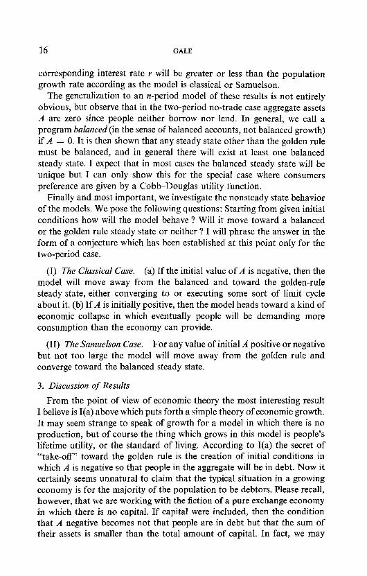
corresponding interest rate Y will be greater or less than the population growth rate according as the model is classical or Samuelson.

The generalization to an n-period model of these results is not entirely obvious, but observe that in the two-period no-trade case aggregate assets A are zero since people neither borrow nor lend. In general, we call a program balanced (in the sense of balanced accounts, not balanced growth) if A = 0. It is then shown that any steady state other than the golden rule must be balanced, and in general there will exist at least one balanced steady state. I expect that in most cases the balanced steady state will be unique but I can only show this for the special case where consumers preference are given by a Cobb-Douglas utility function.

Finally and most important, we investigate the nonsteady state behavior of the models. We pose the following questions: Starting from given initial conditions how will the model behave ? Will it move toward a balanced or the golden rule steady state or neither ? I will phrase the answer in the form of a conjecture which has been established at this point only for the two-period case.

(I) The Ckmsicul Case. (a) If the initial value of A is negative, then the model will move away from the balanced and toward the golden-rule steady state, either converging to or executing some sort of limit cycle about it. (b) If A is initially positive, then the model heads toward a kind of economic collapse in which eventually people will be demanding more consumption than the economy can provide.

(II) The Samuelson Case. For any value of initial A positive or negative but not too large the model will move away from the golden rule and converge toward the balanced steady state.

3. Discussion of Results

From the point of view of economic theory the most interesting result I believe is I(a) above which puts forth a simple theory of economic growth. It may seem strange to speak of growth for a model in which there is no production, but of course the thing which grows in this model is people’s lifetime utility, or the standard of living. According to I(a) the secret of “take-off” toward the golden rule is the creation of initial conditions in which A is negative so that people in the aggregate will be in debt. Now it certainly seems unnatural to claim that the typical situation in a growing economy is for the majority of the population to be debtors. Please recall, however, that we are working with the fiction of a pure exchange economy in which there is no capital. If capital were included, then the condition that A negative becomes not that people are in debt but that the sum of their assets is smaller than the total amount of capital. In fact, we may

PURE EXCHANGE EQUILIBRIUM OF DYNAMIC ECONOMIC MODELS 17

think of our model as including capital implicitly. Fisher in talking about a person’s income stream makes it clear that he thinks of this stream as being to a large extent generated by the person’s capital holdings. With this understanding the negativity of A interpreted as the difference between private assets and capital becomes reasonable, and result I(a) is in accordance with those obtained by Stein [S] and Gale [2, 31.

On the other hand, the result (II) above is in apparent contradiction with assertions made by Samuelson concerning the effect of introducing money into the model. The “contrivance of money,” it seems to me, is exactly a means of making A initially positive. In the two-period model, for instance, if the old people are started out at time 0 with A4 units of money, then the initial value of A is M and hence positive. Samuelson now claims, “Society by using money will go from the nonoptimal negative-interest-rate configuration to the optimal biological-interest-rate configuration.” He goes on, “How does this happen? I shall try to give only a sketchy account that does not pretend to be rigorous.”

My own analysis seems to indicate that such a strategy unfortunately will not work and that following the injection of money the model will not move up toward the golden rule but will as time goes on fall back once again to the nonoptimal balanced equilibrium. True, if M is chosen to be exactly the golden rule value of A, then the model will in one period jump over to the golden rule, and perhaps this is al1 that Samuelson is saying. However, this would be a very risky business, for if one made the mistake of overshooting by making A4 greater than golden rule A then the economy would proceed to destroy itself in the manner described in I(b).

I will conclude this discussion on a somewhat speculative note. The ultimate purpose of economic theory is presumably to explain economic phenomena. What, if anything, can be said about the present exercise in this connection ? Again I would go back to the result I(a). Certainly, rapidly growing economies are objects of actual experience. Our findings suggest that the impetus to growth is given by starting conditions in which the magic number A is negative. If A was initially zero it would take some kind of interference with the competitive mechanism to get things going (we discuss how this might be done in a later section) but the point is that such intervention would in our simplified world only be required once. Thereafter the invisible hand of prices could be allowed to take control and the economy would grow toward the goIden rule optimum. It seems to me not inconceivable that things of this sort may be going on.

In the same spirit, what can be said about the perversely nonoptimal behavior in the Samuelson case ? Here I expect we will look in vain for real Iife examples. While the Samuelson world is perfectly conceivable from a logical point of view it is probably not the one we live in-exactly

18 GALE

because of the empirical facts adduced by Fisher relating to impatience and investment opportunities.

II. THE TWO-PERIOD MODEL

1. Feasible Programs

We consider a population growing geometrically at the rate y so that yt people are born in period t. Each person lives for two periods. People subsist by consuming a good which we shall call income. Each person receives an endowment e = (e O, e,) representing his income in the two periods of his life. All people of all generations are assumed to have identical endowments and preferences.

Let c(t) = (co(t), c,(t + 1)) be the consumption in the two periods of his life of a person born in period t. A program for this model is simply a sequence (c(t)). A program will be calledfeasible if aggregate consumption equals aggregate endowment in each period (we assume income is never thrown away). In period t these aggregates are clearly ++(t) + yt-ICI(t) and yte, + yt-le, so feasibility is given by the equation

r(eo - co(t)) + (el - cl@)> = 0. (1.1)

The quantities e, - cJt> are the savings (or disavings) of a person of age i in period t.

In the analysis to follow we will often be concerned with steady states or stationary programs in which consumption c(t) is independent of time. For this case Eq. (1.1) becomes simply

y(e, - cd + (el - cd = 0. (1*2)

To complete the model we suppose that people have a continuous preference ordering defined on their lifetime consumption vectors. We write as usual c 2 c’ to mean that c is at least as desirable as c’. From continuity of preferences there exists among all stationary feasible programs one (or more) which is most prefered. We call this an optimal stationary program, or in conformity with the current usage, a golden rule program.

2. Competitive and Equilibrium Programs: Steady States

DEFINITION. A program (c(t)) is called competitive if there exists a sequence (pJ of nonnegative numbers called interest factors such that

de0 - co(t)> + (el - 4 + 1)) = 0 (the budget equation) (2.1)

PURE EXCHANGE EQUILIBRIUM OFDYNAMIC ECONOMIC MODELS 19

and

if c>c, then de0 - co) + (el - 4 < 0. (2.2)

This is, of course, the usual condition that consumers maximize utility subject to their budget. The budget Eq. (2.1) says simply the savings earns interest at the rate pt - 1.

Finally, a program which is both competitive and feasible will be called an equilibrium program. These form the subject of the present study.

We consider first the case of stationary equilibria in which c(t) is independent of t. It then follows from (2.1) that pt is also time independent and we have

p(e, - co> + (e, - cd = 0. (2.3)

Subtracting (1 .l) from (2.3) gives

(P - r)(eo - 4 = 0 (2.4)

and we have our first

THEOREM. There are at most two possible steady state equilibria. Either (I) p = y or (II) c, = e, .

The interest of this theorem lies in its interpretation. For the sake of completeness we review the well-known facts.

In Case I we claim the program c is optimal stationary for if there were some prefered stationary program c” then from (2.2)

y(b” - F”) + (bl - 9) < 0

which means that c” is not feasible. Case II is even simpler. It is the case in which each person simply con-

sumes exactly his own endowment and there is no borrowing or lending, i.e., no trade between generations. We can now restate our theorem in words as follows:

THEOREM 1. A steady state equilibrium must be either, (I) an optimal stationary program or (II) a program in which there is no exchange between generations.

Remark. Note that in proving Theorem 1 we used only the market clearing Eq. (1.2) and the budget Eq. (2.3) and made no use of the preference ordering. Thus, the theorem amounts to little more than a bookkeeping identity.

20 GALE

We have seen that there are at most two stationary equilibria. Are there exactly two ? First, note that it is possible for the two equilibria to coincide corresponding to the coincidental case when (e) is an optimal stationary program. From now on we exclude this case. To obtain existence theorems one must, of course, make some assumption such as convexity of preferences. Then existence follows in the usual manner. To get the optimal stationary program consider the “budget line” through e with slope -y and choose the maximal point on this line. To get the no trade program choose p so that the budget line through e is tangent to the “indifference curve” through e. Figure 1 tells the story. The existence proofs are standard and will be omitted.

-

FIGURE 1

Let us now assume that preference orderings are “smooth” and strictly convex. This means that the optimal stationary program is unique. We denote it by C. Also the interest factor associated with the no trade equilibrium is unique. We denote it by p”. In terms of the two stationary equilibria we can now give a precise definition of classical models on the one hand and Samuelson models on the other.

DEFINITION. A model will be called classical (Samuelson) if E,, > e, , 6% < eo>.

In other words, in the classical case people want to consume more than their endowment in their youth and pay it back in their old age. This is, of course, Fisher’s idea of “impatience.”

PURE EXCHANGEEQUILIBRIUM OF DYNAMIC ECONOMIC MODELS 21

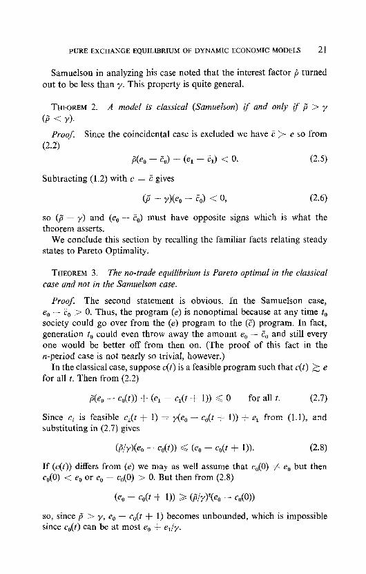
Samuelson in analyzing his case noted that the interest factor p” turned out to be less than y. This property is quite general.

THEOREM 2. A model is classical (Samuelson) if and oniy if p” > y

(p” < Yl

Proof. Since the coincidental case is excluded we have C > e so from (2.2)

p"(eo - F,) + (e, - El) < 0.

Subtracting (1.2) with c = E gives

(2.5)

(P” - r>(eo - 2,) < 0, (2.6)

so (p - y) and (e, - C,,) must have opposite signs which is what the theorem asserts.

We conclude this section by recalling the familiar facts relating steady states to Pareto Optimality.

THEOREM 3. The no-trade equilibrium is Pareto optimal in the classical case and not in the Samuelson case.

Proof. The second statement is obvious. In the Samuelson case, e, - Z;, > 0. Thus, the program (e) is nonoptimal because at any time t, society could go over from the (e) program to the (2) program. In fact, generation t, could even throw away the amount e, - Co and still every one would be better off from then on. (The proof of this fact in the n-period case is not nearly so trivial, however.)

In the classical case, suppose c(t) is a feasible program such that c(t) 2 e for all t. Then from (2.2)

PCe, - c,(t)) + (el - cdt + 1)) 6 0 for all t. (2.7)

Since ct is feasible cl(t + 1) = r(eO - co(t + 1)) + e, from (1 .l), and substituting in (2.7) gives

Wir)(eo - co(t)) G (e. - cdt + 1)). (2.8)

If (c(t)) differs from (e) we may as well assume that c,(O) # e, but then c,(O) < e, or e, - c,(O) > 0. But then from (2.8)

(e. - cdt + 1)) 3 WrWo - co@))

so, since p” > y, e, - c,(t + 1) becomes unbounded, which is impossible since co(t) can be at most e, + e,/y.

22 GALE

3. Nonstationary Programs

We turn now to the study of all equilibrium programs. For this purpose we assume that preferences are given by a utility function u(c) which is concave, increasing and differentiable. People born in period t will then maximize u(c(t)) subject to the budget Eq. (2.1). From (2.1), c,(t + 1) = pt(e, - c,(t)) + e, . At a maximum the derivative of u with respect to q,(t) vanishes and we get

hl(Ct) - Pt%(Ct) = 0 (we here denote c(t) by ct) (3.1)

where U, and u1 are the partial derivatives of u with respect to c,, and c1 . Eliminating pt between (3.1) and (2.1) gives

(e, - h(t)) 444 + (e, - cdt + 1)) h(4 = 0.

Rewriting Eq. (1.1) we have also

(3.2)

(e. - co(tNy + (el - 40) = 0. (3.3)

Equations (3.2) and (3.3) completely describe our dynamical system. Assuming we can solve (3.2) for c1 as a function of c,, , we start with some given nonnegative initial value of c,(O) then use (3.3) to determine c,(O), then (3.2) to determine c,(l) and so on. Of course, there is no guarantee that the ct determined in this way will remain nonnegative. Indeed, as we shall see, certain initial values of c,(O) may lead to a situation in which ct becomes negative corresponding to a kind of breakdown of the economy.

The whole situation is represented graphically in Fig. 2 below.

I I’\- _ infeasible A

\ Classical Case

FIGURE 2

PURE EXCHANGE EQUILIBRIUM OF DYNAMIC ECONOMIC MODELS 23

The straight line AB is the graph of Eq. (1.2) and the curve PQ is the graph of the equation

(e, - cd h(c> + (e, - cl> h(c) = 0. (3.4)

These two loci intersect exactly in the two points giving the two stationary equilibria. One can prove this fact once again by solving (1.2) and (3.4) simultaneously (solve (1.2) for e, - cl and substitute into (3.4)). The figure represents the classical case since T, is greater than e, . To get the Samuelson case one simply interchange the labels e and C.

The figure also gives a graphical representation of the dynamic behavior of the model. We have seen that once the initial value c,(O) is given the dynamic Eqs. (3.2) and (3.3) determine the program forever after. We will be especially interested in initial values c,(O) which are close to e, (if c,(O) = e, we get precisely the no-trade steady state). From our present point of view the number c,(O) is an initial datum presumably given by past history. However, since the model’s future behavior depends so crucially on this number we will devote a later section to discussing the “starting up problem,” -how various initial conditions might come about.

Using Fig. 2 one can easily trace out the programs starting from any initial c,(O). First from (3.3), we get c,(O) and a starting point (c,(O), c,(O)) on line AB. Let us call this vector c”(0) and in general write c”(t) = (c,(f), cl(t)) as contrasted with c(t) = (c,(f), c,(t + 1)). Now clearly c(O) is the point where the vertical line through c”(0) meets curve PQ. (This point is uniquely determined under the assumption that (3.4) can be solved for c1 in terms of c0 , an assumption which will be investigated shortly.) In the same way c”(1) is the intersection of the horizontal line through c(O) and the line AB, and so on. By successive horizontal and vertical jumps, we obtain the whole sequence (c(t)). We also see how a program can become infeasible. This happens precisely if c”(t) lies above the horizontal line through A, for this means that cl(t) exceeds ye, + e, , thus that old people’s demand for consumption exceeds the endowment of the whole economy.

Two cases are represented in the figure. In the first, c,(O) is less than e, so that old people consume less than their endowment. In this case, c(t) moves away from the no-trade pattern and toward the golden rule. It will either converge to the optimal stationary point or approach some limit cycle about it. In the second case, c,(O) exceeds e, so that old people consume more than their endowment. This leads to disaster! The young consume less and less and save more and more until on the fatal day as old people they try to cash in their savings for more consumption than the economy can provide.

24 GALE

We can sum up the situation by saying that for the classical model the optimal stationary program is stable and the no-trade program unstable. For the Samuelson case, of course, it is just the other way around. The no-trade equilibrium is stable while the golden rule is unstable. The picture is given in Fig. 3.

\

=0 B

FIGURE 3

Of course, these pictures do not constitute proofs of the facts we have just asserted. In particular, how can we be sure the curve PQ has been drawn correctly ? At issue are the questions: (i) Can (3.4) be solved for c1 in terms of c0 , and (ii) If so, does PQ lie below AB for c,, between e, and E,, as the pictures indicate. If (i) and (ii) hold then the geometric pictures are easily translated into algebra by the very standard arguments of so-called “cobweb theory.”

We first observe that (i) alway has an affirmative answer at least in some neighborhood of e, for by the implicit function theorem the condition for solvability is that the partial derivative of the left side of (3.4) with respect to c1 at e must not vanish, but this partial derivative is precisely--u,(e) which is not zero since u is assumed to be increasing. The slope of PQ at e is obtained by computing dc,/&, implicitly, giving

the last equality coming from (3.1). But in the classical case, ,6 > y (Theorem 3) so -p” < -y, but -y is the slope of line AB so the assertion

PURE EXCHANGE EQUILIBRIUM OF DYNAMIC ECONOMIC MODELS 25

follows in the classical case. In the Samuelson case p” < y so PQ crosses AB from below as in Fig. 3. We thus see that our drawings are correct at least in the neighborhood of the point e and we get a general “local” result.

THEOREM 4. In the classical case the no-trade equilibrium is unstable. Initial values close to e will produce programs moving away,from e. In the Samuelson case the no-trade equilibrium is locally stable. Initial values close to e will give programs which converge monotonically to e.

What can we say now about gIoba1 behavior of the model ? As regards (i), it might happen, say, that for some value of c,, there are two values of c1 satisfying (3.4) or equivalently that there are two different interest factors which will cause young people to consume the same c,, . Indeed, there are easy examples of utility functions which give rise to first period con- sumptions which are not monotonic in the interest factor. When this occurs, the dynamic system becomes indeterminate since there is no reason for the market to choose one interest factor rather than the other. However, in the classical case the following result is available.

THEOREM 5. In the classical case if the utility function is either (i) separable or (ii) homothetic then (3.4) can be solved (uniquely) for c, for all cO > e, .

Proof. In the separable case u(c) = u(c,,) + w(cl) where v and w are concave, increasing and differentiable functions. (3.4) becomes

v’(co)(co - e3 = w’(c& - 4. (3.5)

For a given cO > e, , the left-hand side of (3.5) is a positive number. For c1 close to zero the right-hand side is large and as c1 increases it decreases strictly to zero as c1 approaches e, . It follows that there is a unique c1 for which (3.5) holds.

For a quasiconcave homothetic utility function it is well known that the ratio u,,(c)/u~(c) is a decreasing function of co/cl . Rewrite (3.4) as

udc>/d4 = (cl - cXco - 4, (3.6)

and note that for a fixed c,, greater than e, the right-hand side of (3.6) is decreasing in c1 and c,/c, is also decreasing so that the left-hand side of (3.6) is increasing and the existence of a unique solution follows.

4. Some Examples

The behavior of the dynamic model is particularly simple if we can show that c1 is determined as a decreasing function of cO by Eq. (3.4) for in this

26 GALE

case one can show, by well-known elementary arguments, that given the right initial condition (ct) will converge monotonically to the golden rule or no-trade programs depending on which of the two cases obtains. In order to get this kind of result we must show that the slope of the curve PQ of Fig. 2 is always negative or equivalently that the normal vector to PQ at each point is positive (has positive coordinates). But the normal vector to PQ is proportional to the gradient of the function on the right-hand side of Eq. (3.4), which gives an easy way of determining the monotone character of PQ.

EXAMPLE 1 (Cobb-Douglas).

It is convenient in this case to choose the unit of income so that e, + e,/y = 1. We then have that the optimal stationary program takes the following simple form:

if = (010 ? Y%),

as one easily verifies. Thus, we are in the classical or Samuelson case according as 01~ is greater or less than e, .

The partial derivatives of u are given by

%3 = ~o/Co 2 Ul = %/Cl

and (3.4) becomes

or

ao(eo/co - 1) + &4c1 - 1) = 0,

oIoeo/co + wl/cl = 1, (4.1)

which represents a rectangular hyperbola. The gradient is proportional to (~oeo/co2, cxlel/c12), so the locus PQ has negative slope as asserted.

EXAMPLE 2 (constant elasticity).

u(c, , Cl> = (%p + ~lc:-“)/(l - P), p > 0, p # 1.

Then the partial derivatives are u. = oio/co4, u1 = al/cla and (3.4) becomes

a,(e, - co)/coB + q(el - clYclE = 0 (4.2)

PUREEXCHANGE EQUILIBRIUM OF DYNAMICECONOMIC MODELS 27

and the gradiant is proportional to

bO@%/4?1 + (1 - Ph% GWclBfl + (1 - B>lcf)l. (4.3)

For p < 1 we again have a positive gradiant. For ,8 > 1 it is possible for the slope of PQ to be positive at the point i;

so that convergence to C will not be monotonic.

EXAMPLE 3 (Quadratic utility). We will treat a special case which shows the possibility of cycling:

u(c, ) Cl) = lOc, - 4c,2 + 4c, - c12,

and we assume the endowment is e = (0, 2) and population is constant. Equation (1.1) is thus

q)(t) = 2 - cl(t) (4.4)

and (3.3) becomes

(5 - 4c,(t)) c,(t) - (2 - c,(t + 1))2 = 0. (4.5)

Eliminating cl(t) gives

(4 + 1)j2 = 5%(t) - 4(C0(t))2. (4.6)

Observe that (4.6) has as its two steady states the no-trade solution c = (0,2) and the golden rule solution C = (1, 1). It also has a solution which is cyclic of period 2. Namely, if c,(t) = (5 - ~‘5)/6, then c,(t + 1) = (5 + ~‘5)/6, c,(t + 2) = (5 - 2/5)/6 and so on, as one can verify by direct substitution in (4.6). Thus, the lifetime consumptions ct oscillate between (0.46, 0.79) and (1.21, 1.54), so generations alternately live above and below the golden rule level.

This is an amusing example of a “business cycle” which has nothing to do with expectations. There are no ex posts or ex antes. Everyone has perfect forsight but cycling nevertheless occurs as a consequence of the equilibrium price mechanism.

5. The Initial Conditions, Some Bookkeeping Problems and Interpretations

In [4] Samuelson states what he calls an “Impossibility Theorem” to the effect that if a model is started not from some initial value c,(O) but at the beginning of “biological” time so that there are no old people but only young people with their endowment e, , then the model will never, following a competitive path, approach the golden rule. For the two-

28 GALE

period model this is a triviality since if initially both e, and c,(O) are zero then the only equilibrium program is the no-trade steady state. More generally, as we have noted, if c,(O) = e, then the no-trade program is the only solution. It seems fair to ask therefore, whether it is economically reasonable to start with c,(O) different from e, .

A related problem is the following: Consider the golden rule steady state. In the classical case, T, > e, so people borrow in the youth and pay back in their old age. Thus, at any moment of time approximately half the population is in debt. But where are the creditors ? There are none. What then has happened to double entry bookkeeping? The same situation occurs in a less obvious way in a model where people live for n periods. In the optimal stationary program each person at each stage of his life may be either a debtor or a creditor, but if we now sum the net assets over the whole population the number we get will, except for coincidence, not be zero and again we have a situation where society as a whole is a debtor or creditor. How do we explain this apparent paradox. Here are several answers;

(A) There is nothing to explain. Book balancing works for the finite time horizon models to which we are accustomed but, as we have seen, it may not be possible in open-ended models. While I believe this answer is technically correct, it does seem desirable to work out an accounting system which will preserve the traditional bookkeeping properties. Here are two ways in which this can be done.

(B) Introduce credit or debt in the initial conditions. Suppose first that c,(O) < e, . This means that in period zero old people consume less than their endowment. It is then quite reasonable to make the convention that these old people have a credit equal to e, - c,(O) of consumption, but this is a credit they will never cash in since they die after consuming their c,(O). Accordingly, the credit remains on the books forever and just cancels out the debt which as we observed is owed by the population as a whole. In the other case, when c,(O) exceeds e, the old people have consumed more than their endowment and hence owe c,(O) - e, . At this point, however, they die but their debt lives on forever and the holders of the debt are the living population at each point of time. Of course, the debt cannot be collected since the debtors are dead (and have left no estate), but that’s all right because at the equilibrium interest rate people don’t want to collect the debt anyway. (This last situation corresponds to Samuelson’s contriv- ance of money. This will be seen even more clearly in connection with the next illustration.)

The above suggests a “story” to explain how the given initial conditions might come about. Suppose, for example, we are in the classical case. The

PURE EXCHANGE EQUILIBRIUM OF DYNAMIC ECONOMIC MODELS 29

model has been running along for some time in the no-trade equilibrium but at time t = 0 some of the old people realize that if they are willing to give up ever so little of their second period consumption the economy in the future will move up toward the golden rule. Accordingly, they take a part E of their endowment e, and put it up “for sale.” The market mechanism does the rest and as our analysis has shown consumption moves up toward the golden rule. (By our bookkeeping rules the bene- factors are given a credit of E which, of course, will in each period be assumed to earn interest at the going rate, and everything balances out.)

If this altruistic scenario sounds too unrealistic, one can instead imagine a central authority which levies an income tax on the old people in period zero and then sells this income back to the young. The thing to note once again about this type of “intervention” is that it need be done only once! After that the government can simply sit back pursuing a laissez-faire policy and watch the standard of living climb.

(C) The central clearing house. Here we describe a device which is frequently used in explaining equilibrium even in the static case. We suppose that people never trade directly with each other but work through a clearing house. Thus, suppose c,(O) is less than e, . Then the amount of income e, - c,(O) is held by th e c earing house. The new generation of 1 young people wish to consume this excess and must therefore buy it from the clearing house. Of course, they will not be able to pay for it until their old age. Accordingly, they leave with the clearing house an I.O.U. for e, - c,(O) units of income. In the next period they pay their debt (with interest) and get the I.O.U. back which they can then destroy. But, of course, in the mean time a new generation of young people has come to the clearing house with a new collection of I.O.U.‘s and so on, so at each instant of time the clearing house is holding I.O.U.‘s in exactly the amount of the debt owed by the population.

In the other case with c,(O) > e, we have young people selling an amount e, - c0 to the clearing house and this time it is the clearing house which gives the young people the I.O.U.‘s to cash in their old age. Once again the books balance because the population now holds the debt (1.0.U.‘~) issued by the clearing house. This last, it seems to me is precisely Samuelson’s contrivance of money.

Suppose then that we are in the Samuelson case and that the clearing house is also a government which wants to move the economy from the no-trade to the golden rule steady state. For this purpose in period t = 0 the government simply “coins” an I.O.U. worth E units and hands it to the old people. The market interest rate then adjusts so that the young people will want to sell precisely E units, and the economy is off of dead

30 GALE

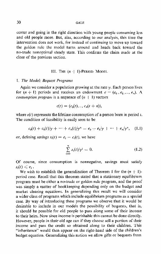
center and going in the right direction with young people consuming less and old people more. But, alas, according to our analysis, this time the intervention does not work, for instead of continuing to move up toward the golden rule the model turns around and heads back toward the no-trade nonoptimal steady state. This confirms the claim made at the close of the previous section.

III. THE (n + l)-PERIOD MODEL

1. The Model: Bequest Programs

Again we consider a population growing at the rate y. Each person lives for (n + 1) periods and receives an endowment e = (e, , e, ,..., e,). A consumptioil program is a sequence of (n + 1) vectors

4) = (co(t),..., 4 + 4),

where c(t) represents the lifetime consumption of a person born in period t. The condition of feasibility is easily seen to be

coo> + m/Y + *-. + c,(t)/yTl = e, + e,/y + a** + en/f, (1.1)

or, defining savings si(t) = ei - ci(t), we have

m

2 s,(t)/yi = 0. i=O

(1.2)

Of course, since consumption is nonnegative, savings must satisfy Si(t) < e, .

We wish to establish the generalization of Theorem 1 for the (n + l)- period case. Recall that this theorem stated that a stationary equilibrium program must be either a no-trade or golden rule program, and the proof was simply a matter of bookkeeping depending only on the budget and market clearing equations. In generalizing this result we will consider a wider class of programs which include equilibrium programs as a special case. By way of introducing these programs we observe that it would be desirable to include in our models the possibility of bequests, that is, it should be possible for old people to pass along some of their income to their heirs. Now since income is perishable this cannot be done directly. However, people in their old age can if they choose sell a portion of their income and pass the credit so obtained along to their children. This “inheritence” would then appear on the right-hand side of the children’s budget equation. Generalizing this notion we allow gifts or bequests from

PURE EXCHANGE EQUILIBRIUM OF DYNAMIC ECONOMIC MODELS 31

people of any age in one period to people in the next period. The models considered heretofore correspond to the special case in which people of age i(i < n) bequeath their entire fortune to people of age i + 1 in the next period. In that case the inheritors are simply the donnors one period later.

Formally, let a,(t) denote the assets in period t of a person at the beginning of the i-th period of his life. (For the models without bequests a,(t) would simply be the value of the accumulated savings of a person during the first i periods of his life.) It is assumed that in period t the person of age i saves (or dissaves) an additional amount s,(t) (where s?(t) = e, - c,(t)) so that his assets a,‘(t) at the end of period t are given by

where pt is the interest factor of period t. At the end of period t the person must then determine how he will distribute his assets among the people of period t + 1. Let c+(t) be the amount which this person passes on to people of agej in period t + 1. The only rule is that each person must pass on all of his assets. This is the “budget equation”

j$ %At) = PtQi(t) + s,(t), (1.4)

Equation (1.4) represents what might be called the conservation of wealth, asserting that assets are neither created nor destroyed. We will call a program satisfying (1.4) a bequest program.

The total assets A(t) of society in period t is the sum of the assets of all the individuals. Since those are yt-i people of age i this gives

A”(t) = 1 yt-iat(t) (all sums are henceforth assumed to run from 0 to n).

If we normalize by dividing by yt we get aggregate assets A(t) in period t defined by

A(t) = c aJt)/y”. (1.5)

The basic identity which we shall need describes how aggregate assets change with time.

LEMMA. For any bequest program,

A0 + 1) = (PJY) A(t).

642/6/l-3

(1.6)

32 GALE

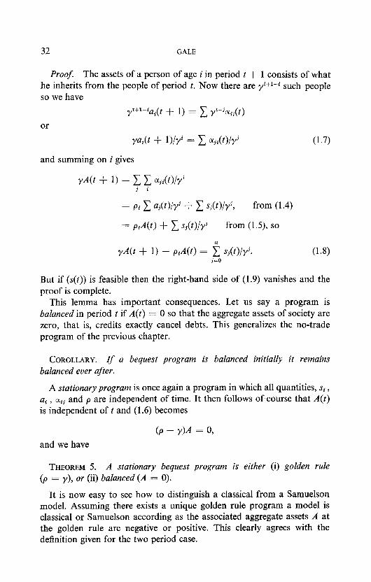
Proof. The assets of a person of age i in period t + 1 consists of what he inherits from the people of period t. Now there are yt+l-i such people so we have

or

p-ia,(t + 1) = 1 yt%&)

ya& + l>/r” = c %i(W

and summing on i gives

(1.7)

from (1.4)

= PtA@) + c s&>/r’ from (1.5), so

yA(t + 1) - ptA(t) = i sj(t)/y. j=O

(1.8)

But if (s(t)) is feasible then the right-hand side of (1.9) vanishes and the proof is complete.

This lemma has important consequences. Let us say a program is balanced in period t if A(t) = 0 so that the aggregate assets of society are zero, that is, credits exactly cancel debts. This generalizes the no-trade program of the previous chapter.

COROLLARY. If a bequest program is balanced initially it remains balanced ever after.

A stationary program is once again a program in which all quantities, si , ai , olij and p are independent of time. It then follows of course that A(t) is independent of t and (1.6) becomes

and we have

THEOREM 5. A stationary bequest program is either (i) golden rule @ = y), or (ii) balanced (A = 0).

It is now easy to see how to distinguish a classical from a Samuelson model. Assuming there exists a unique golden rule program a model is classical or Samuelson according as the associated aggregate assets A at the golden rule are negative or positive. This clearly agrees with the definition given for the two period case.

PURE EXCHANGE EQUILIBRIUM OF DYNAMIC ECONOMIC MODELS 33

In [4] Samuelson argues for his special three-period model that if the model is started out at the beginning of “biological time,” so that there are young people but no middle aged or old people, then the equilibrium program will not approach the golden rule. (He also gives a numerical example in which the program approaches a nongolden rule balanced steady state.) He refers to this as “The Impossibility Theorem.” Our present analysis shows that this impossibility theorem holds quite generally, for in the beginning of biological time clearly aggregate assets are zero and hence must remain so ever after. But in the golden rule program aggregate assets will not be zero (except by coincidence), so no balanced program can approach the golden rule, and, in fact, any balanced program must be bounded away from the golden rule program in all time periods.

Actually it seems a bit far fetched to consider programs starting with Adam and Eve (there is nothing in the scriptures to indicate that prices go back that far). A more reasonable starting point would be the beginning of “economic time,” namely, the day on which God or someone else created prices. Let us imagine that up to that time everyone in every period simply consumed his own endowment because there was no mechanism for facilitating borrowing and lending. Thus, initially there were no debtors or creditors. After a few periods of trading, of course, the situation changed with some people becoming creditors and others debtors. Nevertheless, from our Corollary the sum of the debts and credits would have to remain zero as long as there was no intervention with the free bequest mechanism and therefore it would be impossible for society to evolve toward the golden rule optimum.

2. Steady State Equilibria

In the previous section it was shown that any stationary bequest program is either golden rule or balanced. Nothing was said there about existence of either kind of program, however, and to study this question we now return to consideration of equilibrium programs. We limit ourselves to the stationary situation.

For any interest factor p let c(p) = (c,,(p),..., en(p)) be the consumption vector chosen by a consumer to maximize his lifetime preference ordering subject to his budget equation

C ci(p>/p” = C c/pi, (2.1) or equivalently,

c SiCPYP” = 0, (2.2)

where si(p) = ei - c<(p).

34 GALE

In this notation, Eq. (1.8) becomes

(Y - p> A(P) = c Si~PW- (2.3)

Under the assumption of strictly convex preferences there will be a unique vector c(p) for each positive interest factor p and c(p) will vary continuously with p. In particular, for p = y we get the golden rule equilibrium program c(y) which almost by definition is optimal stationary [any preferred stationary program would violate the budget Eq. (2.1) which, since p equals y, is the same as the feasibility Eq. (1. l)]. What is more interesting, however, is the fact that under very mild assumptions there will also always exist at least one balanced program. Let us denote the right-hand side of (2.3) by (b(p). W e must show that d(p) has at least two roots. This follows from the following:

LEMMA. If the endowment vector e has at least two positive coordinates and Q-preferences are increasing, then 4(p) is negative for p close to 0 and also for p close to co.

Proof (sketch). Let m be the smallest index i such that e, is positive and let M be the largest such index. If p is extremely large, then consumption ci for i > m becomes almost a free good so consumers will demand more than the economy can provide. Similarly, if p is very small then consump- tion ci for i < M is essentially free and again consumption demand will exceed endowment. In each case then s(p) will be negative.

THEOREM 6. Under the assumption of the Iemma there always exists at least one balanced steady state. Further, if the model is classical (Samuelson) there is a balanced steady state with interest factor p” greater than (less than)

Y*

Proof. (i) Classical Case, A(y) < 0. Then for p slightly greater than y, (r - p) A(p) = 4(p) is positive. But C(p) is negative for large p; hence by continuity A(p) = 0 for some p > y.

(ii) Samuelson Case, A(y) > 0. Then for p slightly less than y, (y - p) A(p) = $(p) is again positive, but $(p) is negative for p sufficiently small and the conclusion follows as before.

(iii) Coincidental Case, A(y) = 0. Then the golden rule program is balanced (by definition).

Although I have not been able to establish any general result I believe the usual situation is that there exists exactly one balanced steady state.

PURE EXCHANGE EQUILIBRIUM OF DYNAMIC ECONOMIC MODELS 35

In any case this is easy to show for the Cobb-Douglas utility function where preferences are given by a utility function II defined by

u(co )...) c,) = 2 ai log ci , oii > 0, 1 ai = I. (2.4)

Maximizing (2.4) subject to (2.1) gives

(2.5)

as one easily verifies, and thus

so

and

From Theorem 6 we know that 4(p) has at least two positive roots. But the polynomial on the right of (2.6) has at most two such roots. This follows from Descartes rule of signs which says that the number of positive roots of a polynomial cannot exceed the number of changes of sign of its coefficients. Note that all coefficients of (2.6) are negative except for the coefficient of pn. Hence there are only two sign changes and therefore at most two roots and we have exactly one balanced steady state as asserted.

It would of course be very interesting to establish stability results like those of the previous chapter for the (n + 1)-period case. While I believe analogous theorems hold at least in the Cobb-Douglas case, I have not yet succeeded in proving them.

REFERENCES

1. I. FISHER, “The Theory of Interest,” Augustus M. KelIey, New York, 1961.

2. D. GALE, General equilibrium with imbalance of trade, J. Znt. Econ. 1 (1971), 141-158.

3. D. GALE, “On Equilibrium Growth of Dynamic Economic Models,” ORC 71-2, Operations Research Center, University of California, Berkeley, CA, February 1971.

36 GALE

4. P. A. SAMUELSON, “An Exact Consumption-Loan Model of Interest with or without the Social Contrivance of Money,” J. Pol. Econ. 66 (1958), 467482.

5. J. L. STEIN, “A Minimal Role of Government in Achieving Optimal Growth,” Economica, May (1969), 139-150.

6. D. STARRETT, On golden rules, the biological theory of interest and copetitive inefficiency, J. Pal. Econ., to appear.