PURDUE UNIVERSITY GRADUATE SCHOOL Thesis/Dissertation …€¦ · · 2017-07-30GRADUATE SCHOOL...
51
Graduate School Form 30 Updated 1/15/2015 PURDUE UNIVERSITY GRADUATE SCHOOL Thesis/Dissertation Acceptance This is to certify that the thesis/dissertation prepared By Entitled For the degree of Is approved by the final examining committee: To the best of my knowledge and as understood by the student in the Thesis/Dissertation Agreement, Publication Delay, and Certification Disclaimer (Graduate School Form 32), this thesis/dissertation adheres to the provisions of Purdue University’s “Policy of Integrity in Research” and the use of copyright material. Approved by Major Professor(s): Approved by: Head of the Departmental Graduate Program Date Xiaoxiao Zhang CFD Analysis of Hotmetal Desulfurization Process for Improved Mixing in a Torpedo Vessel Master of Science in Engineering Chenn Zhou Chair Bipin K. Pai Xiuling Wang Chenn Zhou George Nnanna 4/22/2015
Transcript of PURDUE UNIVERSITY GRADUATE SCHOOL Thesis/Dissertation …€¦ · · 2017-07-30GRADUATE SCHOOL...

Graduate School Form 30Updated 1/15/2015
PURDUE UNIVERSITYGRADUATE SCHOOL
Thesis/Dissertation Acceptance
This is to certify that the thesis/dissertation prepared
By
Entitled
For the degree of
Is approved by the final examining committee:
To the best of my knowledge and as understood by the student in the Thesis/Dissertation Agreement, Publication Delay, and Certification Disclaimer (Graduate School Form 32), this thesis/dissertation adheres to the provisions of Purdue University’s “Policy of Integrity in Research” and the use of copyright material.
Approved by Major Professor(s):
Approved by:Head of the Departmental Graduate Program Date
Xiaoxiao Zhang
CFD Analysis of Hotmetal Desulfurization Process for Improved Mixing in a Torpedo Vessel
Master of Science in Engineering
Chenn ZhouChair
Bipin K. Pai
Xiuling Wang
Chenn Zhou
George Nnanna 4/22/2015


CFD ANALYSIS OF HOTMETAL DESULFURIZATION PROCESS FOR
IMPROVED MIXING IN A TORPEDO VESSEL
A Thesis
Submitted to the Faculty
of
Purdue University
by
Xiaoxiao Zhang
In Partial Fulfillment of the
Requirements for the Degree
of
Master of Science in Engineering
May 2015
Purdue University
Hammond, Indiana

All rights reserved
INFORMATION TO ALL USERSThe quality of this reproduction is dependent upon the quality of the copy submitted.
In the unlikely event that the author did not send a complete manuscriptand there are missing pages, these will be noted. Also, if material had to be removed,
a note will indicate the deletion.
All rights reserved.
This work is protected against unauthorized copying under Title 17, United States CodeMicroform Edition © ProQuest LLC.
ProQuest LLC.789 East Eisenhower Parkway
P.O. Box 1346Ann Arbor, MI 48106 - 1346
ProQuest 1602898
Published by ProQuest LLC (2015). Copyright of the Dissertation is held by the Author.
ProQuest Number: 1602898

ii
ii
ACKNOWLEDGEMENTS
This is a great opportunity to express my gratitude to those who have guide me, support
me and provide me this great research opportunity.
The greatest thanks go to Prof. Chenn Zhou, who offered me the opportunity to study in
Purdue and guide me to start my research work. I would also like to thank Prof. Xiuling
Wang and Prof. Bipin Pai for being on my advisory committee and for their helpful
suggestions.
I would like to thank Center for Innovation through Visualization and Simulation (CIVS)
for providing me this great working place and all the resources required for this work.
Especially my supervisor Mr. Bin Wu and Mr. Armin Silaen for their guidance on the
projects.
I would also like to thank ArcelorMittal USA for offering this opportunity, providing
funding, and tor comceptual guidance during the course of this work.

iii
iii
TABLE OF CONTENTS
Page
TABLE OF CONTENTS ................................................................................................... iii
LIST OF TABLES ............................................................................................................. iv
LIST OF FIGURES ............................................................................................................ v
NOMENCLATURE ......................................................................................................... vii
ABSTRACT ....................................................................................................................... ix
CHAPTER 1. INTRODUCTION ....................................................................................... 1
1.1 Background .............................................................................................................. 1
1.2 Literature Review ..................................................................................................... 3
1.3 Objectives................................................................................................................. 4
CHAPTER 2. NUMERICAL MODEL ESTABLISHMENT ............................................ 6
2.1 Methodology ............................................................................................................ 6
2.2 Geometry and Boundary Conditions...................................................................... 12
CHAPTER 3. RESULTS AND DISCUSSION ................................................................ 14
3.1 Base Case Analysis ................................................................................................ 15
3.2 Effect of Lance Position ......................................................................................... 21
3.3 Effects of Gas Flow Rate ....................................................................................... 23
3.4 Effect of Nozzle Diameter ..................................................................................... 25
3.5 Effect of Rotating Lance ........................................................................................ 27
3.6 Mixing Time Comparison among Seven Cases ..................................................... 29
CHAPTER 4. CONCLUSIONS ....................................................................................... 31
LIST OF REFERENCES .................................................................................................. 32
APPENDIX ....................................................................................................................... 34

iv
iv
LIST OF TABLES
Table .............................................................................................................................. Page
Table 1 Simulation/solver settings .................................................................................... 12
Table 2 Boundary conditions and material properties ...................................................... 13
Table 3 Case matrix .......................................................................................................... 14
Table 4 Mixing time comparison among nine cases ......................................................... 30

v
v
LIST OF FIGURES
Figure Page
Figure 1 Computational geometry of the torpedo vessel used
for desulfurization contents............................................................................................... 13
Figure 2 Initial conditions in the torpedo vessel ............................................................... 15
Figure 3 The location of three chosen planes for monitoring velocities........................... 15
Figure 4 The area-averaged velocities at different planes as a function of
simulation time.................................................................................................................. 16
Figure 5 (a) Liquid iron distribution and (b) velocity vectors at 30 s ............................... 17
Figure 6 Contours of velocity at different horizontal planes inside the bath (30 s).......... 18
Figure 7 (a) Initial tracer position in the torpedo vessel and
(b) evolution of the mixing process .................................................................................. 19
Figure 8 Evolution of the mixing index (M) for the base case ......................................... 20
Figure 9 Comparison of velocity vectors: (1) Base case (b) Case 2 (c) Case 1 ................ 21
Figure 10 Comparison of mixing times for different lance immersions
(Base case, Case 1 and Case 2) ......................................................................................... 22
Figure 11 Comparison of velocity vectors for various gas flow rates
[(a) Case 3, (b) Base case, (c) Case 4] .............................................................................. 23

vi
vi
Figure Page
Figure 12 Comparison of mixing times for various gas flow rates
(Base case, Case 3 and Case 4) ......................................................................................... 24
Figure 13 Comparison of velocity vectors for various nozzle diameters
[(a) Case 5, (b) Base case, (c) Case 6] .............................................................................. 25
Figure 14 Comparison of mixing times for various nozzle diameters
(Base case, Case 5 and Case 6) ......................................................................................... 26
Figure 15 Geometry of case 7 (rotating lance) ................................................................. 27
Figure 16 The area-averaged velocities at different planes as a function of
simulation time.................................................................................................................. 28
Figure 17 Comparison of velocity vectors between case 7 and base case
[(a) Case 7, (b) Base case] ................................................................................................ 28
Figure 18 Comparison of mixing time (Case 7 and Base case) ........................................ 29

vii
vii
NOMENCLATURE
D Nozzle diameter
F External body force
g̅ Gravitational acceleration
Gb Generation of turbulence kinetic energy due to buoyancy
Gk Generation of turbulence kinetic energy due to the mean velocity
gradients
H Bath height
Ι Unit tensor
k Turbulence kinetic energy
M Mixing index
MFR Mass flow rate of nitrogen
P Static pressure
Poutlet Gauge pressure at outlet
Sε, 𝑆𝐾 User-defined source term, which is zero in k-ɛ model
Sm Mass source term
T Temperature
V⃗⃗ Velocity vector
u, v, w Velocities on the coordinate axes (x,y,z)

viii
viii
YM Contribution of the fluctuating dilatation in compressible turbulence
to the overall dissipation rate
q qth fluid's volume fraction in the cell
Coefficient of thermal expansion
ε Dissipation of turbulent kinetic energy
ρ Fluid density
τ Stress tensor
Molecular viscosity
t Turbulent viscosity
∇ Gradient
Cμ, C1, C2, C1ε, C2ε Constants in turbulence k-ɛ model
σo, 𝜎 Standard deviation of tracer concentration at time 0 second and at
current time
σk, σε Turbulent Prandtl number for k and ɛ

ix
ix
ABSTRACT
Zhang, Xiaoxiao. M.S.E., Purdue University, May 2015. CFD Analysis of Hotmetal
Desulfurization Process for Improved Mixing in a Torpedo Vessel. Major Professor: Chenn
Q. Zhou.
A torpedo car is an elongated cylindrical vessel, which is widely used in steel plants to
transfer liquid iron from the blast furnace to the melt shop and perform desulfurization
process. Removing the sulfur contained in pig iron is very important to meet the stringent
quality criteria required in the downstream processes. The desulfurization process is
performed in a torpedo vessel during the transportation by injecting desulfurizing reagents
into the liquid iron with nitrogen as the carrier gas. An optimization of this process is
desired to improve the desulfurization efficiency. In this study, a 3-D computational fluid
dynamics (CFD) model has been developed to analyze the flow field in the liquid iron bath
inside a torpedo vessel. Parametric studies were conducted to assess the opportunities to
improve the efficiency of the desulfurization process.

1
1
CHAPTER 1. INTRODUCTION
1.1 Background
A torpedo car (sometimes called a torpedo ladle car) is widely used in the steel industry.
The hot metal from blast furnace is tapped into a torpedo vessel and the vessel is transferred
on a rail car from the cast house to a desulfurization station prior to its delivery to the melt
shop. Generally, a torpedo vessel has a horizontal cylindrical shape with conical ends (refer
to Figure 1). The liquid iron is transferred through an opening at the top of the vessel. The
inside of the torpedo vessel is lined with insulating refractory bricks to hold the liquid iron,
protect the outer steel shell and to minimize heat loss from the vessel.
New product development for special applications (such as line pipe) calls for stringent
quality control at the liquid steel stage. In order to meet the requirements of steelmaking
quality for advanced applications, the sulfur concentration in the hot metal needs to be less
than 0.005%1. The demand for much lower sulfur in the final product is increasing rapidly
due to the need for improved mechanical properties (such as toughness and formability)
and better surface quality and internal characteristics.

2
2
During hot metal desulfurization in a torpedo, a multi-hole lance is lowered into the liquid
iron through the opening at the top of the torpedo car. The desulfurization reagent particles
are injected with a carrier gas into the hot metal to achieve a stirring action that promotes
mass transfer. The reagent spreads in the liquid iron or attaches to the surface of the carrier
gas bubbles, and then reacts with the sulfur to form a sulfide product that floats out to the
metal-slag interface for removal2. A typical reaction involving calcium diamide (CaC2 or
CaD) and Mg powder as the reagent is given below:
CaC2(s) Ca(v) + 2[C] (R1)
Ca(v) + [S] CaS(s) (R2)
Mg(v) + 2[C] MgC2(s) (R3)
The magnesium consumes the carbon released from CaD so that the desulfurization
reaction can proceed with the dissociation of CaD to release Ca (the main desulfurizer).
The desulfurization in torpedo is a mixing controlled process (the dimensionless
Damkohler number can be used to assess the competition between mixing rate and reaction
rate in this vessel). Near the lance, the mixing should be generally good (and hence reaction
will be favorable) but there are dead-zones away from the lance that needs to be stirred so
that new reactants can be transported in those areas to react with sulfur in the hot metal and
the product of reaction can be advected away to continue the reaction. The reacting surface
can be renewed only by stretching and folding of fluid volumes15. In dead-zones, fluids
will mix by diffusion which is a much slower process than convection (external stirring).
Therefore, it is required to find an optimum configuration that will provide more stirring

3
3
and hence lower mixing time. The current work employs numerical experimentation
through computational fluid dynamics (CFD) to simulate the flow field of liquid iron in a
torpedo vessel. Once a quasi-steady state is reached, a tracer dispersion study (on the frozen
steady-state flow field) is carried out to obtain a mixing index that characterizes the
homogeneity of the bath as a function of time. This characterization tool is then used to
perform what-if scenarios to explore the parameter space, and determine favorable
configurations for desulfurization.
1.2 Literature Review
Huang et al.1 simulated the fluid flow in a torpedo vessel by using an Eulerian multiphase
model. This vessel was fitted with porous plugs in the bottom for additional stirring and a
porous media model was applied for the gas flow through the porous refractory. In this
work, the desulfurization process was studied numerically and it was reported that the
process was improved by increasing the gas flow rate, in addition to using bottom blowing.
Pehlke and Fuwa3 outlined the influence of sulfur on the quality and property of steel
products. Different desulfurization reagents were introduced in this article and different
methods to control sulfur in liquid iron and steel were discussed. Silva et al.4 investigated
the influence of different desulfurizing reagents and several operational variables on hot
metal desulfurization. Seshadri et al.2 developed a kinetic model for the molten pig iron
desulfurization by injection of lime-based powders. The process of the reactant powder
reagents dispersing in the melt or attaching to the bubble-metal interface has been discussed
in this paper. Zou et al.5 discussed the hot metal desulfurization by powder injection using

4
4
a mathematical model; and Irons and Guthrie6 studied the kinetics of molten iron
desulfurization using magnesium vapor. Yugov et al.7-8 introduced sulfur removal
problems and the equipment, technologies and desulfurization methods used at
metallurgical plants. Dyudkin et al.9 reported that the most effective desulfurization method
to achieve a low content of sulfur in pig iron is the usage of magnesium-bearing reagents.
The mechanism of the desulfurization by granulated magnesium is discussed in this article.
Resulfurization mechanism during magnesium desulfurization of molten iron was
investigated by Yang et al.10. Lange11 introduced the operations, reactions and reactors of
secondary steelmaking processes. The mechanisms, benefits and potentialities of these
processes under the application of thermodynamic and kinetic principles have been
discussed. Quinn et al.12, Bhattacharya et al.13, and recently Dan et al.14, have used a
multivariate data-driven approach to model the desulfurization process in a torpedo vessel
and predict key process variables such as reagent consumption.
1.3 Objectives
The purpose of this study is to investigate the mixing process inside a torpedo car. A
detailed flow field in the vessel will be simulated by using Computational Fluid Dynamics
(CFD) technology. A 3-Dimensional model will be developed by using CFD solver Fluent
14.0. The model simulated by using current operating conditions will be validated with the
field data. Computational experiments will be conducted by changing operating conditions
and geometry and other parameters related to the mixing efficiency.
5
5
The objective of this thesis is to develop a detailed CFD model of a torpedo vessel. The
flow field will be established first and mixing study will be conducted later. The mixing
time obtained under the specific operating conditions will be validated with the field
experiment data. A series of parametric studies will be conducted based on this base case.
The influence of related parameters on the mixing time will be investigated by comparing
with base case.
The detailed of objectives are:
Build a 3 Dimensional geometric model according the drawing provided by the
steelmaking plant;
Develop a 3 Dimensional multi-phase model of a torpedo vessel under specific
operating conditions;
Investigate the mixing process after having a steady state flow field;
Conduct parametric studies to find the influence of mass flow rate, nozzle direction,
lance depth and nozzle diameter on the mixing time;
Compare the mixing time obtained under different operating condition and come
up with an optimal plan to improve the mixing process.
6
6
CHAPTER 2. NUMERICAL MODEL ESTABLISHMENT
2.1 Methodology
The commercial finite volume code ANSYS FLUENT 14.016 was used to solve the
governing equations (partial differential equations for momentum and continuity). The
volume of fluid (VOF) model was used to simulate the multiphase flow in the torpedo
vessel. The hot metal was considered as the primary phase and nitrogen (carrier gas) as the
secondary phase in the VOF model. The powder (reagent) was not explicitly modeled as
the flow is inertia driven and we are only interested in mixing due to the stirring action of
the gas. Once a quasi-steady state is reached, a tracer dispersion study on the frozen flow
field is carried out to obtain a mixing index that characterizes the homogeneity of the bath
as a function of time. Turbulence was modeled using the realizable k- model.
Governing equations
The governing equations solved in the simulation are presented below.
Conservation of mass
∇ ∙ (ρV⃗⃗ ) = Sm (1)

7
7
Conservation of momentum
∇ ∙ (ρV⃗⃗ V⃗⃗ ) = −∇p + ∇ ∙ (τ̿) + ρg̅ + F̅ (2)
where P is the static pressure, ρg̅ and F are the gravitational body force and external body
force, respectively, and τ is the stress tensor, which is given by:
τ̿ = μ [(∇V⃗⃗ + ∇V⃗⃗ T) −2
3∇ ∙ V⃗⃗ I] (3)
In equation 3 above, is the molecular viscosity, Ι is the unit tensor, and the second term
on the right hand side is the effect of volume dilation.
Turbulence model
Due to the presence of zones with high Reynolds number inside the torpedo vessel, the
realizable k-ε model, which is based on model transport equations for the turbulence kinetic
energy (k) and its dissipation rate (ε), is employed. The realizable k- turbulence model is
used due to its robustness and economy. It is a semi-empirical model based on the transport
equation for the turbulence energy (k) as given below:
∂
∂t(ρk) +
∂
∂xi(ρkuj) =
∂
∂xj[(μ +
μt
σk)
∂k
∂xj] + Gk + Gb − ρε − YM + SK (4)

8
8
μt = Cμρk2
ε (5)
The generation of kinetic energy and buoyance force attribution are:
Gk = −ρui′u′
j̅̅ ̅̅ ̅̅ ̅̅ ∂uj
∂xi (6)
Gb = βgiμt
Prt
∂xi
∂T (7)
The turbulent dissipation rate () is expressed as,
∂
∂t(ρε) +
∂
∂xi(ρεui) =
∂
∂xj[(μ +
μt
σε)
∂ε
∂xj] + ρC1Sε − ρC2
ε2
k+√νε+ C1ε
ε
kC2εGb + Sε (8)
where the equations are given for xj direction. Gk is the generation of turbulence kinetic
energy due to the mean velocity gradients. Gb is the generation of turbulence kinetic energy
due to buoyancy. YM represents the contribution of the fluctuating dilatation in
compressible turbulence to the overall dissipation rate. SK and Sε are user-defined source
terms, set to zero in this model.
VOF model
The VOF formulation relies on the fact that two or more fluids or phases are not
interpenetrating. For each additional phase, a new variable is introduced such as the volume

9
9
fraction of the phase in the computational cell. In each control volume, the sum of volume
fractions of all phases is unity.
The fields for all variables and properties are shared by the phases and represent volume-
averaged values, as long as the volume fraction of each of the phases is known at each
location. Thus the variables and properties in any given cell are either purely representative
of one of the phases, or representative of a mixture of the phases, depending upon volume
fraction values.
gas + steel = 1 (9)
In other words, if the qth fluid's volume fraction in the cell is denoted as 𝑞 , then the
following three conditions are possible:
• 𝑞= 0: the cell is empty (of the qth fluid).
• 𝑞= 1: the cell is full (of the qth fluid).
• 0<𝑞< 1: the cell contains the interface between the qth fluid and one or more other fluids.
The volume-fraction-averaged density takes on the following form:
ρ = gasρgas + steelρsteel (10)
The volume-fraction-averaged viscosity is computed in the following manner:

10
10
μ = gasμgas + steelμsteel (11)
The VOF function 𝑔satisfies Eq. (12).
∂
∂t(g) + ∇ ∙ (αgV⃗⃗ ) = 0 (12)
Simulation process
As mentioned earlier, the simulation process could be divided into two parts: (a) flow
simulation and (b) mixing study.
Flow simulation
The liquid iron and gas were considered stationary in the initial condition. The carrier
gas is then injected through the lance nozzles into the bath. The strong jets will slowly
stir the liquid iron and establish a fully developed flow. Liquid velocities at various
locations are monitored during the calculations. The calculations are stopped after the
flow has reached a quasi-steady state.
Mixing study
Once the flow field has reached a quasi-steady state, a tracer – which has the same
properties as the liquid iron – is introduced in the area under the lance. Then, only the
transient species transport equation is solved, which has a convection and diffusion term.
In order to evaluate the mixing process, the tracer concentration is monitored throughout
11
11
the simulation. For each time step, a mixing index M, as defined below, is calculated. The
mixing index is related to the standard deviation of the tracer concentration and is given
by,
M = (1 −σ
σo) (13)
where is the standard deviation of the tracer concentration in the whole domain at any
time t, and o is standard deviation of the tracer concentration at time t = 0 s. As an initial
condition, a rectangular area under the lance is patched with the tracer (i.e., the
concentration of the tracer species is set to 1.0) whereas the tracer concentration in other
areas is set to zero. When the mixing process completes, the tracer concentration will be
uniform throughout the domain and hence the standard deviation of tracer concentration in
the domain will become very small (close to zero). Therefore, M will asymptotically
assume a value of 1.0 when the mixing is completed as per equation 13. A user-defined
function (UDF) in ANSYS FLUENT was used to calculate the standard deviation ( 𝜎) of
the tracer during the mixing process. Table 2.1 lists the simulation/solver settings used in
this study.

12
12
Table 1 Simulation/solver settings
Pressure-Velocity Coupling Scheme PISO
Transient Formulation First Order Implicit
Spatial Discretization Schemes
Gradient: Least Squares Cell Based
Pressure: PRESTO!
Momentum: Second Order Upwind
Volume Fraction: First Order Upwind
Turbulent Kinetic Energy: First Order Upwind
Turbulent Dissipation Rate: First Order Upwind
Energy: Second Order Upwind
2.2 Geometry and Boundary Conditions
Figure 1 shows the computational domain that was reproduced from the engineering
drawing of the torpedo vessel. The inlet and outlet boundaries have been shown in Figure
1. Only the fluid volume (bath + gas above the bath) inside the vessel is modeled. The two
inlet nozzles are located at the bottom of the lance and are oriented at 45º from the
horizontal long axis of the vessel. The nozzle position is dictated by the lance immersion
depth in the torpedo car and is generally close to the bottom of the vessel in order to stir
the liquid iron bath effectively. The nitrogen gas, which carries the desulfurizing reagent
particles, is injected into the bath through the inlets.

13
13
Table 2 shows the boundary conditions and material properties used in this simulation. The
carrier gas (nitrogen) is injected into the hot metal through the inlets at the mass flow rate
of MFR. A zero gauge pressure is assigned as the pressure at the torpedo car outlet (Poutlet).
A no slip boundary condition is applied on the walls and on the lance’s surface. In the base
case, the nitrogen gas is injected from each nozzle at the same flow rate.
Table 2 Boundary conditions and material properties
Boundary Conditions:
Inlets Mass Flow Rate: MFR*
Outlet Gauge Pressure: Poutlet = 0 Pa
Walls No slip (v = 0 m/s)
Material Properties:
Liquid iron density (kg/m3) 7000
Nitrogen density (kg/m3) 2.8
Liquid iron viscosity (kg/m-s) 0.0055
Liquid iron temperature (°C) 1500
*refer to the nomenclature section at the end
Figure 1 Computational geometry of the torpedo vessel used for desulfurization contents

14
14
CHAPTER 3. RESULTS AND DISCUSSION
Table 3 shows the various cases that were studied as part of the parametric analysis to
optimize the process. A base case was chosen to evaluate the desulfurization process under
typical operating conditions. Further to the base case analysis, seven parametric cases were
carried out where four parameters (lance immersion depth, gas flow rate, nozzle diameter
and rotating lance) were varied. The mixing efficiency of each parametric case was
compared to that of the base case.
Table 3 Case matrix
Case Lance position (mm)
(Depth from liquid
level)
Gas flow
rate (kg/s)
Nozzle
diameter
(mm)
Lance
motion
Base Case Hlp MFR D Fixed
1 1/3 × Hlp MFR D Fixed
2 2/3 × Hlp MFR D Fixed
3 Hlp MFR × 1.5 D Fixed
4 Hlp MFR × 0.5 D Fixed
5 Hlp MFR 1.25 × D Fixed
6 Hlp MFR 0.75 × D Fixed
7 Hlp MFR D Rotating
*refer to the nomenclature section at the end

15
15
3.1 Base Case Analysis
The base case has been simulated under the typical operating conditions. Figure 2 shows
the initial conditions in the torpedo vessel. The pink shaded area represents the liquid iron
and the light blue area represents the gas phase. The liquid level or bath height (H) is also
shown in Figure 2.
In order to confirm that a steady flow field has been obtained, three planes (Figure 3)
located at different heights inside the liquid iron bath have been chosen to monitor the area-
averaged velocity. When the area-averaged velocity of each plane reached a quasi-steady
value, the flow field is considered to have reached a steady state.
Figure 4 shows the average velocities on the three planes as the simulation progresses.
Prior to 15 s, the average velocities change significantly as the time progresses.
Figure 2 Initial conditions in the torpedo vessel
Figure 3 The location of three chosen planes for monitoring velocities

16
16
Subsequently, the area-averaged velocities settle gradually and do not change significantly.
During this period, the flow field can be assumed to be quasi-steady.
Figure 4 The area-averaged velocities at different planes as a function of simulation time

17
17
Figure 5 (a) Liquid iron distribution and (b) velocity vectors at 30 s
The flow field at 30 s has been chosen as the starting velocity field for the mixing study as
the flow field is fully developed and is considered to be steady. Figure 5 shows the liquid
iron distribution and the velocity vectors on the vertical middle plane and also on a vertical
45o plane inside the torpedo vessel. It can be observed from Figure 5a that the nitrogen gas,
when injected into the bath, flows upward around the lance periphery and forms a plume.
The velocity vector plots show a large recirculation zone on a vertical plane and two

18
18
opposing recirculation zones located on each side of the lance symmetrically when viewed
on a 45o plane (Figure 5b, black arrows).
Figure 6 shows the velocity distribution on various horizontal planes at different bath
heights. Nearly stagnant zones were observed at each end of the torpedo vessel, which may
have negative effects on the efficiency of the desulfurization process due to poor mixing.
These corner areas are considered as the potential areas where mixing could be enhanced
by modifying the process parameters including lance designs.
Figure 6 Contours of velocity at different horizontal planes inside the bath (30 s)

19
19
Figure 7 (a) Initial tracer position in the torpedo vessel and
(b) evolution of the mixing process
From a fluid dynamics perspective, the desulfurization process can be regarded as the
stretching and folding of the fluid elements inside the bath due to the stirring action of the
nitrogen gas injected through the lance. A good mixing would ensure uniform dispersion
of the desulfurization reagent and efficient sulfur removal reaction by continuous surface
renewal so that fresh reactants can arrive at the reaction zone and the product of reaction
can be taken away. In order to study this process, as described earlier, the flow field is
frozen in a typical simulation and a tracer species is introduced at a pre-defined location
20
20
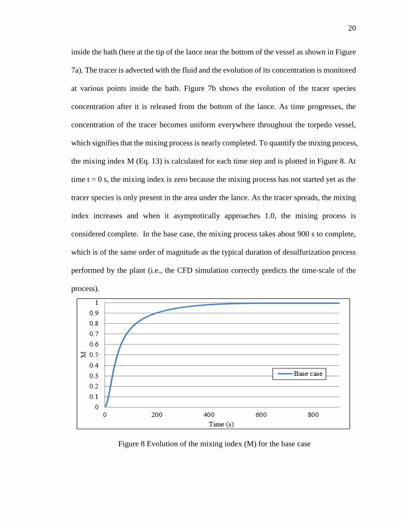
inside the bath (here at the tip of the lance near the bottom of the vessel as shown in Figure
7a). The tracer is advected with the fluid and the evolution of its concentration is monitored
at various points inside the bath. Figure 7b shows the evolution of the tracer species
concentration after it is released from the bottom of the lance. As time progresses, the
concentration of the tracer becomes uniform everywhere throughout the torpedo vessel,
which signifies that the mixing process is nearly completed. To quantify the mixing process,
the mixing index M (Eq. 13) is calculated for each time step and is plotted in Figure 8. At
time t = 0 s, the mixing index is zero because the mixing process has not started yet as the
tracer species is only present in the area under the lance. As the tracer spreads, the mixing
index increases and when it asymptotically approaches 1.0, the mixing process is
considered complete. In the base case, the mixing process takes about 900 s to complete,
which is of the same order of magnitude as the typical duration of desulfurization process
performed by the plant (i.e., the CFD simulation correctly predicts the time-scale of the
process).
Figure 8 Evolution of the mixing index (M) for the base case

21
3.2 Effect of Lance Position
The effect of lance position on the bath mixing has been studied parametrically. In the base
case, the lance tip almost reaches the bottom of the torpedo vessel and the nozzles are very
close to the bottom (see Table I). In case 1, the lance is moved up to a position where the
nozzles are located at 1/3rd of the liquid iron bath height. In case 2, the nozzles are at 2/3rd
bath height.
Figure 9 compares the velocity vectors between the three cases above (base case, case 1
and case 2). As the lance depth decreases (case 1), the gas injection location moves up and
hence the active flow area reduces due to the fact that the gas primarily stirs the bath above
the nozzles. One can observe from Figure 9 that the high velocity area has reduced in case
Figure 9 Comparison of velocity vectors: (1) Base case (b) Case 2 (c) Case 1
22
22
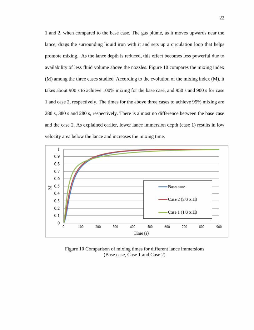
1 and 2, when compared to the base case. The gas plume, as it moves upwards near the
lance, drags the surrounding liquid iron with it and sets up a circulation loop that helps
promote mixing. As the lance depth is reduced, this effect becomes less powerful due to
availability of less fluid volume above the nozzles. Figure 10 compares the mixing index
(M) among the three cases studied. According to the evolution of the mixing index (M), it
takes about 900 s to achieve 100% mixing for the base case, and 950 s and 900 s for case
1 and case 2, respectively. The times for the above three cases to achieve 95% mixing are
280 s, 380 s and 280 s, respectively. There is almost no difference between the base case
and the case 2. As explained earlier, lower lance immersion depth (case 1) results in low
velocity area below the lance and increases the mixing time.
Figure 10 Comparison of mixing times for different lance immersions
(Base case, Case 1 and Case 2)

23
23
3.3 Effects of Gas Flow Rate
In order to understand the effect of gas flow rates on mixing, a parametric study with
varying gas flow rates has been conducted. The mass flow rates for two additional cases
(cases 3 and 4) were fixed at 1.5 × MFR and 0.5 × MFR, respectively, where MFR denotes
the mass flow rate for the base case.
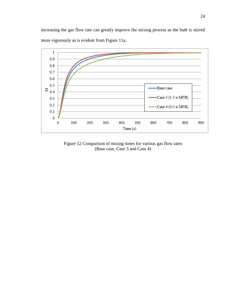
Figure 11 shows the velocity vectors among the three cases (base case, case 3 and case 4).
It is obvious that case 3 has the desirable flow field because it has a larger high velocity
area (less dead zones) compared to the base case and case 4. As shown in Figure 12, it
takes about 500 s and 950 s for case 3 and case 4, respectively, to finish the mixing process.
Also, for cases 3 and 4, 95% mixing is achieved in 230 s and 420 s, respectively. Therefore,
Figure 11 Comparison of velocity vectors for various gas flow rates
[(a) Case 3, (b) Base case, (c) Case 4]
24
24
increasing the gas flow rate can greatly improve the mixing process as the bath is stirred
more vigorously as is evident from Figure 11a.
Figure 12 Comparison of mixing times for various gas flow rates
(Base case, Case 3 and Case 4)
25
25
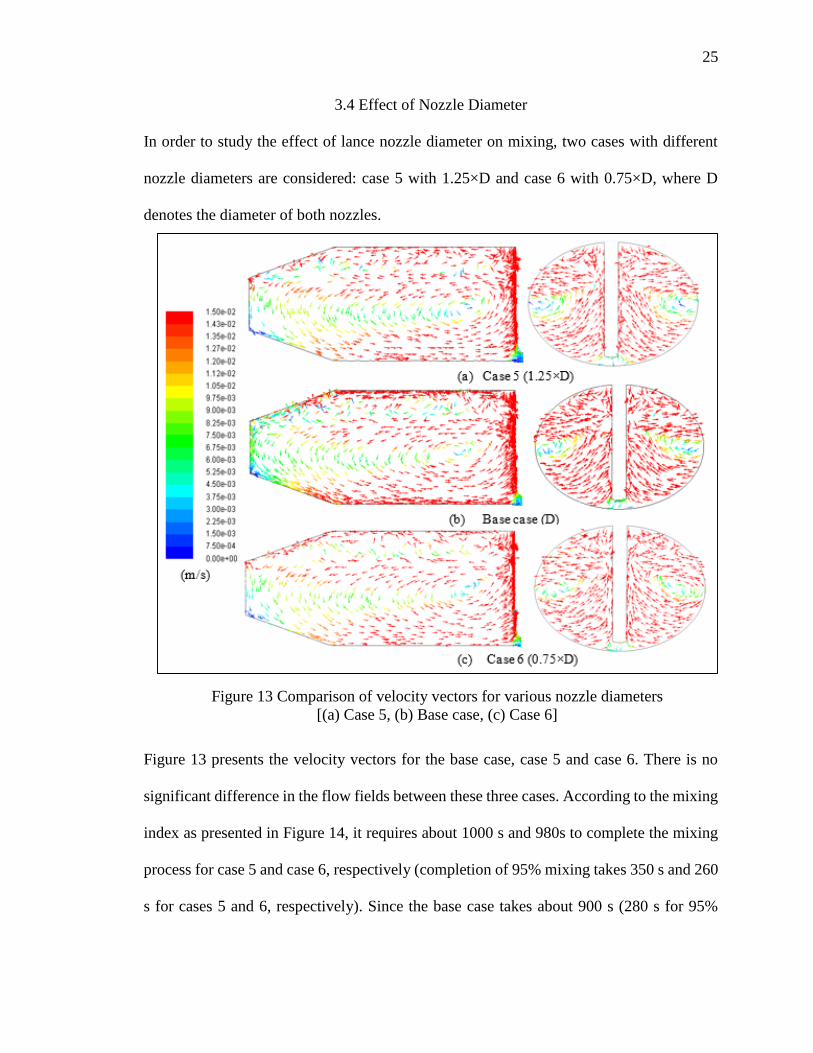
3.4 Effect of Nozzle Diameter
In order to study the effect of lance nozzle diameter on mixing, two cases with different
nozzle diameters are considered: case 5 with 1.25×D and case 6 with 0.75×D, where D
denotes the diameter of both nozzles.
Figure 13 presents the velocity vectors for the base case, case 5 and case 6. There is no
significant difference in the flow fields between these three cases. According to the mixing
index as presented in Figure 14, it requires about 1000 s and 980s to complete the mixing
process for case 5 and case 6, respectively (completion of 95% mixing takes 350 s and 260
s for cases 5 and 6, respectively). Since the base case takes about 900 s (280 s for 95%
Figure 13 Comparison of velocity vectors for various nozzle diameters
[(a) Case 5, (b) Base case, (c) Case 6]
26
26
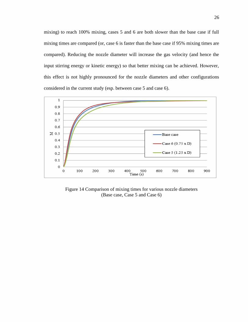
mixing) to reach 100% mixing, cases 5 and 6 are both slower than the base case if full
mixing times are compared (or, case 6 is faster than the base case if 95% mixing times are
compared). Reducing the nozzle diameter will increase the gas velocity (and hence the
input stirring energy or kinetic energy) so that better mixing can be achieved. However,
this effect is not highly pronounced for the nozzle diameters and other configurations
considered in the current study (esp. between case 5 and case 6).
Figure 14 Comparison of mixing times for various nozzle diameters
(Base case, Case 5 and Case 6)
27
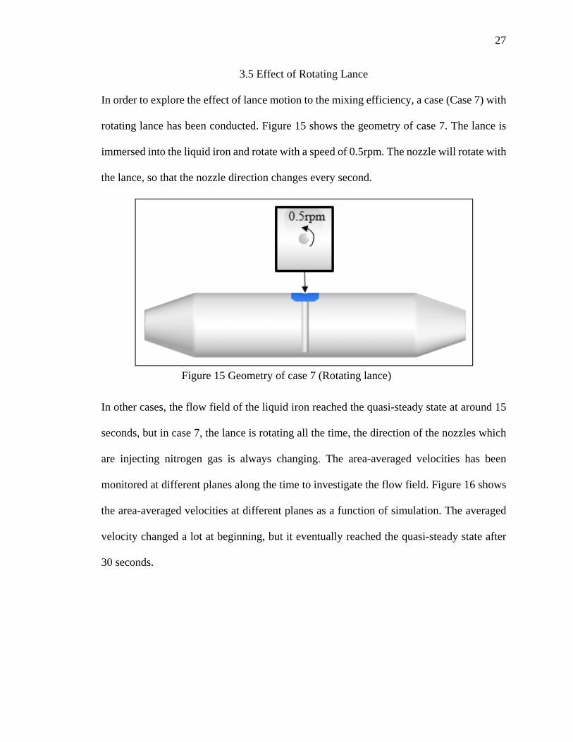
3.5 Effect of Rotating Lance
In order to explore the effect of lance motion to the mixing efficiency, a case (Case 7) with
rotating lance has been conducted. Figure 15 shows the geometry of case 7. The lance is
immersed into the liquid iron and rotate with a speed of 0.5rpm. The nozzle will rotate with
the lance, so that the nozzle direction changes every second.
In other cases, the flow field of the liquid iron reached the quasi-steady state at around 15
seconds, but in case 7, the lance is rotating all the time, the direction of the nozzles which
are injecting nitrogen gas is always changing. The area-averaged velocities has been
monitored at different planes along the time to investigate the flow field. Figure 16 shows
the area-averaged velocities at different planes as a function of simulation. The averaged
velocity changed a lot at beginning, but it eventually reached the quasi-steady state after
30 seconds.
Figure 15 Geometry of case 7 (Rotating lance)

28
28
Figure 17 Comparison of velocity vectors between case 7 and base case
[(a) Case 7, (b) Base case]
Figure 16 The area-averaged velocities at different planes
as a function of simulation time

29
29
Figure 17 shows the comparison of velocity vectors between case 7 and base case. The
flow pattern is almost the same, the low velocity area in case 7 is a little bigger than the
one in base case. By comparing the mixing process (Figure 18), the mixing time for case 7
to achieve 100% mixing is about 960s (900s for base case). Correspondingly, the mixing
time for case 7 to achieve 95% mixing is 260s (230s for base case). The mixing efficiency
is a little lower than the base case. The mixing process is not improved by rotating the lance.
Figure 18 Comparison of mixing time (Case 7 and Base case)
3.6 Mixing Time Comparison among Seven Cases
The mixing times for the seven cases as discussed earlier have been presented in Table 4.
They have been ordered in this table according to their efficiency of the mixing process
with case 3 yielding the fastest mixing time of all cases. By comparing with the other cases,

30
30
the flow field of the liquid has been improved. Correspondingly, the desulfurization
efficiency is also improved in case 3.
Table 4 Mixing time comparison among nine cases
Case Mixing Time (100%) Mixing Time (95%)
3 500s 230s
Base Case 900s 280s
2 900s 280s
1 950s 380s
4 950s 420s
7 960s 260s
6 980s 260s
5 1000s 350s
Case 3 (highlighted in yellow in Table 4), with 50% more gas flow than the base case,
needs the least amount of time to finish both the 100% and 95% mixing. Among all the
parameters considered in this study, gas flow rate has the dominant effect on mixing and
hence it is expected that a higher gas flow rate would result in a better desulfurization
process.

31
31
CHAPTER 4. CONCLUSIONS
The objective of this project is to explore ways to improve the efficiency of the
desulfurization process from a fluid dynamics perspective. A CFD model has been
developed that provides a good three-dimensional (3D) representation of the torpedo vessel.
The simulation results show that there are low velocity areas (dead-zones) at both ends of
the torpedo vessel that could cause poor mixing. By increasing the mass flow rate of the
carrier gas, the flow field could be well improved, and mixing could be promoted. Mixing
time could be cut by as much as 50% if the gas flow rate is increased by 50% for the specific
configuration studied in this work. In order to complement the mixing study, chemical
reactions involved in the desulfurization process will be added to the model. It is expected
that the results of this study will provide recommendations on how to improve the
efficiency of the desulfurization process and guide plant trials.

LIST OF REFERENCES

32
32
LIST OF REFERENCES
1. A. Huang, M. Zhang, H. Gu, “Simulation and optimization of melted iron
desulfurization process in torpedo with blowing gas and spray,” Advanced
Materials Research, Vol. 462, February 2012, pp. 413–418.
2. V. Seshadri, C.A. da Silva, I.A. da Silva, P. von Krüger, “A kinetic model applied
to the molten pig iron desulfurization by injection of lime-based powders,” ISIJ
International, Vol. 37, No. 1, 1997, pp. 21–30.
3. R.D. Pehlke and T. Fuwa, “Control of sulphur in liquid iron and steel,”
International Metals Reviews, Vol. 30, No. 3, 1985, pp. 125–140.
4. S.N. Silva, F. Vernilli, S.M. Justus, C.M. dos S. Araújo, E. Longo, J.A. Varela,
J.M.G. Lopes, B.V. de Almeida, “Selection of desulfurizing agents and
optimization of operational variables in hot metal desulfurization,” Steel Research
International. 84, No. 1, 2013.
5. Z. Zou, Y. Zou, L. Zhang, N. Wang, “Mathematical model of hot metal
desulphurization by powder injection,” ISIJ International, Vol. 41, 2001, pp. S66–
S69.
6. G.A. Irons and R.I.L. Guthrie, “The kinetics of molten iron desulfurization using
magnesium vapor,” Metallurgical Transactions B, Vol. 12B, December 1981, pp.
755–767.

33
33
7. P.I. Yugov and A.L. Romberg, “Improving the quality of pig iron and steel,”
Metallurgist, Vol. 47, Nos. 1–2, 2003.
8. P.I. Yugov, A. Romberg, D. Yang, “Desulfurization of pig iron and steel,
Metallurgist,” Vol. 44, Nos. 11–12, 2000.
9. D.A. Dyudkin, S.E. Grinberg, S.N. Marintsev, “Mechanism of the desulfurization
of pig iron by granulated magnesium,” Metallurgist, Vol. 45, Nos. 3–4, 2001.
10. J. Yang, M. Kuwabara, T. Teshigawara, M. Sano, “Mechanism of resulfurization
in magnesium desulfurization process of molten iron,” ISIJ International, Vol. 45,
No. 11, 2005, pp. 1607–1615.
11. K.W. Lange, “Thermodynamic and kinetic aspects of secondary steelmaking
processes,” International Materials Reviews, Vol. 33, No.2, 1988, pp. 53–89.
12. S.L. Quinn and V. Vaculik, “Improving the desulfurization process using adaptive
multivariate statistical modeling”, AISE Steel Technology, October 2002, pp. 37–
41.
13. T. Bhattacharya, S. Nag, S.N. Lenka, “Analysis of DS reagent consumption using
multivariate statistical modeling”, Tata Search, 2004, pp. 215–223.
14. B. Dan, K. Chen, L. Xiong, Z. Rong, J. Yi, “Research on multi-BP NN-based
control model for molten iron desulfurization,” World Congress on Intelligent
Control and Automation, June 2008, pp. 6133–6137.
15. J.M. Ottino, “The kinematics of mixing: stretching, chaos, and transport,”
Cambridge University Press, 1989.
16. ANSYS FLUENT Theory Guide, ANSYS, Inc., 2011.

APPENDIX

34
34
APPENDIX
Mixing M Index UDF
/* This UDF calculates the standard deviation of tracer concenctration and prints it to a
file */
#include "udf.h"
int LiquidDomainIndex = 1;
DEFINE_EXECUTE_AT_END(StdDev)
{
Domain *d = Get_Domain(1); /* Mixture domain */
Domain *dl =DOMAIN_SUB_DOMAIN(d,LiquidDomainIndex); /* Liquid
domain */
Thread *t;
face_t f;
cell_t c;

35
35
FILE *fp;
float i = 0.;
float Conc = 0.;
float mass_weight=0;
float ConcDiff = 0.;
float ConcAvg, StdDeviation;
real xc[ND_ND];
fp = fopen ("StdDev.txt", "a+");
thread_loop_c(t,dl) {
begin_c_loop(c,t) {
C_CENTROID(xc,c,t);
if (xc[2]<519.5 ) {
Conc +=
C_YI(c,t,0)*C_VOF(c,t)*C_R(c,t)*C_VOLUME(c,t); /* Sums average of tracer in liquid
bath */
mass_weight += C_VOF(c,t)*C_R(c,t)*C_VOLUME(c,t);
i += 1.;
}
}
end_c_loop(c,t)
}
#if RP_NODE
36
36
Conc = PRF_GRSUM1(Conc);
mass_weight = PRF_GRSUM1(mass_weight);
i = PRF_GRSUM1(i);
#endif
ConcAvg = Conc/mass_weight; /* Calculates average of tracer */
thread_loop_c(t,dl) {
begin_c_loop(c,t) {
C_CENTROID(xc,c,t);
if (xc[2]<519.5) {
ConcDiff += pow(((C_YI(c,t,0)-
ConcAvg)*C_VOF(c,t)*C_R(c,t)*C_VOLUME(c,t)),2.); /* Calculates difference of local
tracer concentration to average concentration and sums them up */
}
}
end_c_loop(c,t)
}
printf("ConcAvg %e \n", ConcAvg);
#if RP_NODE
ConcDiff = PRF_GRSUM1(ConcDiff);
#endif
printf("ConcDiff %e \n", ConcDiff);
StdDeviation = pow((ConcDiff/mass_weight),0.5); /* Calculates standard
deviation */

37
37
node_to_host_float_1(StdDeviation);
#if !RP_NODE
fprintf(fp,"%f %e \n", CURRENT_TIME,StdDeviation);
#endif
printf("StdDeviation %e \n", StdDeviation);
fclose(fp); }