71

Economic AnAlysis & Policy, Vol. 41 no. 1, mArch 2011

Purchasing Power Parity (PPP) of Australian Dollar: Do Test Procedures Matter?

AFM Kamrul Hassan Department of Banking and Finance

University of Rajshahi Bangladseh

and

Ruhul Salim* School of Economics and Finance

Curtin University, 78 Murray Street, Perth, WA, 6000, Australia

(E-mail: ruhul.salim@cbs.curtin.edu.au)

Abstract: This article aims to reexamine whether Australia’s real exchange rate is mean reverting in the long run by using quarterly trade weighted indices of real exchange rate data for the period of June 1970 to September 2009. We use the state of the art of several more recent econometric tests for this purpose. The empirical result shows that the non-stationarity of Australia’s real exchange rate cannot be rejected. Thus, our results support the PPP hypothesis in Australia. Our results are contradictory to those of Cuestas and Regis (2008), but conform to those of Darné and Hoarau (2007 and 2008).

I. InTRODuCTIOnPurchasing power parity (PPP) is probably one of the oldest and most debated hypotheses in International Economics. The origin of this hypothesis has been traced back to the writings of the scholars in the fifteenth and sixteenth centuries (Sarno and Taylor 2002). One of the implications of the purchasing power parity (PPP) hypothesis is that the real exchange rate should be stationary, which implies that any shock to the real exchange rate is temporary or short-lived, in the long-run it reverts to its mean value. There are a large number of studies that attempt to identify whether the real exchange rate is stationary. Despite this being the most extensively researched issue, no consensus has yet been reached. It, thus, remains an ongoing area of empirical research. Australia is one of the major commodity exporting countries in the world. Because of this commodity dependency Australian dollar has come to be known as * Corresponding author.1 For an extensive coverage of this issue please see Rogoff (1996) and Sarno and Taylor (2002).

PurchAsing PowEr PArity (PPP) of AustrAliAn DollAr: Do tEst ProcEDurEs mAttEr?

72

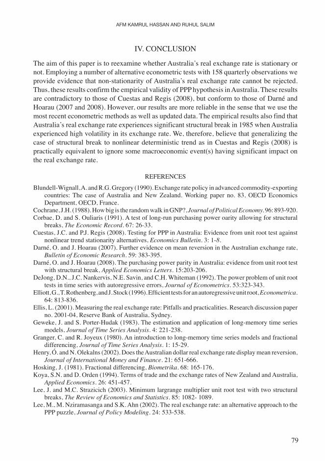
‘commodity currency’. This commodity dependence has given rise to a closer link between its terms of trade and the real exchange rate. Plots of terms of trade and the real exchange rate indices (Figure A1 in the Appendix) show that movements in the trade weighted index of the real exchange rate and terms of trade follow very similar fashion. This close association has been empirically validated and it indicates that the shocks to Australian real exchange rate are permanent. A number of studies have confirmed this non-mean-reverting property of Australia’s real exchange rate, such as, Corbae and Ouliaris (1991), Lee et al. (2002), Henry and Olekalns (2002), Darné and Hoarau (2007 and 2008). Despite this much supported view that Australia’s real exchange rate is not mean-reverting, very recently Cuestas and Regis (2008) reignite the issue by arguing that shocks to Australia’s real exchange rate is short-lived and it reverts to its mean value in the long-run. Thus, the aim of this article is to contribute to this debate by employing a number of econometric tests and more recent data.

This paper differs from previous studies that find stationarity of the Australia’s real exchange rate in several aspects. First, we use most recent and larger quarterly dataset then the previous studies. Second, we use the most relevant measure of the real exchange rate, namely trade weighted real exchange rate. Henry and Olekalns (2002) argued that trade weighted real exchange rate provides wider view of the conditions facing Australian dollar than bilateral real exchange rate. Therefore, studies that use bilateral real exchange rate and find it stationary (such as Tawadros 2002) may not capture the behavior of Australia’s real exchange rate properly. Third, we use relatively recent unit root test with structural break that overcomes the limitation of widely used Perron (1997) test. Fourth, we employ joint variance ratio test that provides overall test statistics instead of test statistic at individual lags as in Olekalns and Wilkins (1998). This facilitates the decision on whether the series, as a whole, exhibits mean-reversion. Finally, in regard to fractional integration, we use Phillips (1999a and 1999b) test with null d = 12 in addition to other two tests used in Olekalns and Wilkins (1998), namely Geweke and Porter-Hudak (1983) and Robinson (1995) test with null d = 0. This adds to the robustness of our results. The overall finding of our analyses indicates that Australia’s real exchange rate does not exhibit mean-reversion property.

The rest of the paper proceeds as follows. Section II, provides a discussion on real exchange rate data followed by empirical estimation and analysis of results in Section III. Conclusions are provided in final section.

II. REAL ExCHAnGE RATE DATA

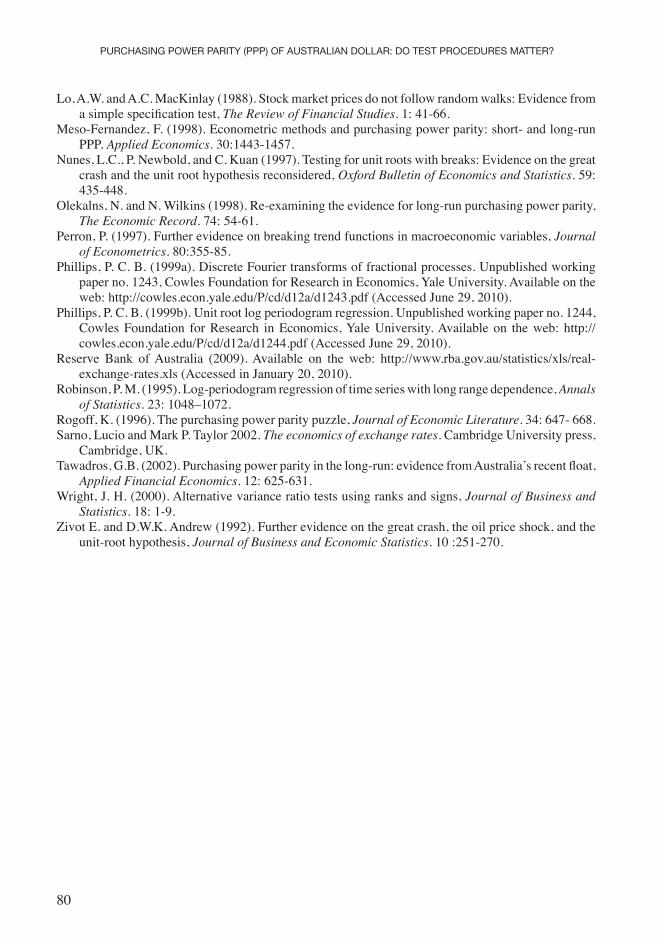
This paper uses quarterly data on Trade Weighted Index (TWI) of the real exchange rate of Australian dollar over the period June 1970 to September 2009. This index is constructed by the Reserve Bank of Australia (RBA) and the procedure of how this index is constructed is described in Ellis (2001). RBA also constructs two other indices: Export Weighted Index (EWI) and Import Weighted Index (IWI). However, as these three indices move in similar fashion (Appendix Figure A2), TWI is used because of its wide application in empirical research.

2 d is differencing parameter. More on this is in Section IV.

Afm KAmrul hAssAn AnD ruhul sAlim

73

III. EMPIRICAL RESuLTS

There are two approaches to test the PPP hypothesis: cointegration of nominal exchange rate with the difference between domestic and foreign price levels and stationarity of the real exchange rate. When nominal exchange rate and price level differences are found to be cointegrated, the real exchange rate is assumed to be stationary and it is said the PPP holds. However, Maeso-Fernandez (1998) notes that if there is long-run relationship between prices and the nominal exchange rate, the real exchange rate can still be non-stationary. ‘The parameters of the cointegrating relationship can be far away from those predicted by the PPP hypothesis’ (Maeso-Fernandez 1998, p. 1447) and for this reason we follow the second approach of using the real exchange rate data to check for mean reversion.

Sarno and Taylor (2002) identify three approaches that are used in PPP literature to test for stationarity of the real exchange rate: (i) unit root tests, such as Augmented Dickey-Fuller (ADF) and Phillips-Perron (PP); (ii) variance ratio test, and (iii) fractional integration. In this paper we choose to follow all three approaches to arrive an unambiguous conclusion on the mean-reversion property of Australian real exchange rate.

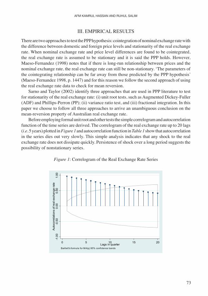
Before employing formal unit root and other tests the simple correlogram and autocorrelation function of the time series are derived. The correlogram of the real exchange rate up to 20 lags (i.e. 5 years) plotted in Figure 1 and autocorrelation function in Table 1 show that autocorrelation in the series dies out very slowly. This simple analysis indicates that any shock to the real exchange rate does not dissipate quickly. Persistence of shock over a long period suggests the possibility of nonstationary series.

Figure 1: Correlogram of the Real Exchange Rate Series

-1.0

0-0

.50

0.00

0.50

1.00

Auto

corre

latio

ns o

f rea

l exc

hang

e ra

te

0 5 10 15 20Lags in quarter

Bartlett's formula for MA(q) 95% confidence bands

PurchAsing PowEr PArity (PPP) of AustrAliAn DollAr: Do tEst ProcEDurEs mAttEr?

74

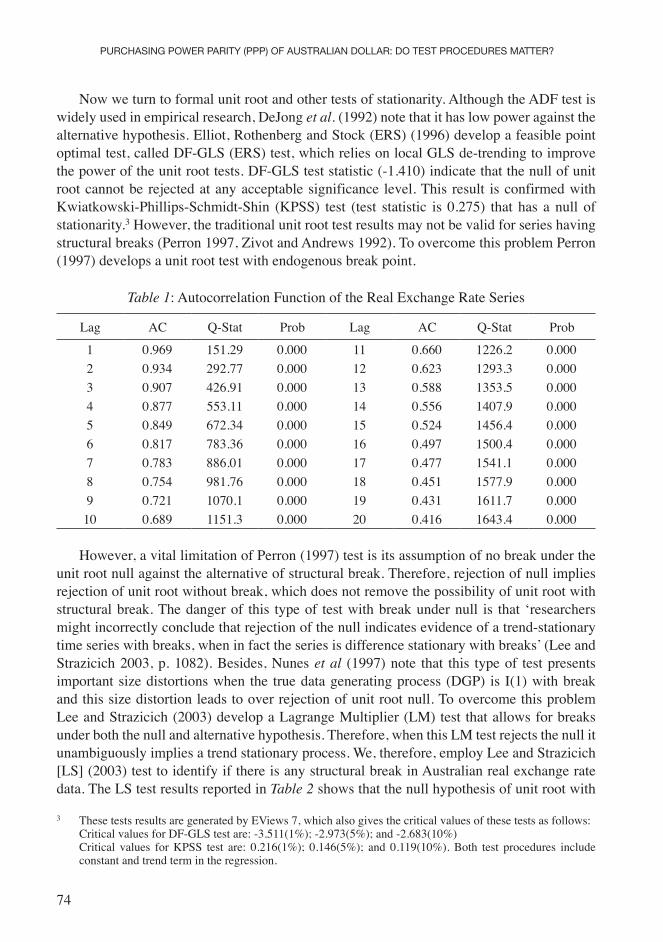
now we turn to formal unit root and other tests of stationarity. Although the ADF test is widely used in empirical research, DeJong et al. (1992) note that it has low power against the alternative hypothesis. Elliot, Rothenberg and Stock (ERS) (1996) develop a feasible point optimal test, called DF-GLS (ERS) test, which relies on local GLS de-trending to improve the power of the unit root tests. DF-GLS test statistic (-1.410) indicate that the null of unit root cannot be rejected at any acceptable significance level. This result is confirmed with Kwiatkowski-Phillips-Schmidt-Shin (KPSS) test (test statistic is 0.275) that has a null of stationarity.3 However, the traditional unit root test results may not be valid for series having structural breaks (Perron 1997, Zivot and Andrews 1992). To overcome this problem Perron (1997) develops a unit root test with endogenous break point.

Table 1: Autocorrelation Function of the Real Exchange Rate Series

Lag AC Q-Stat Prob Lag AC Q-Stat Prob

1 0.969 151.29 0.000 11 0.660 1226.2 0.0002 0.934 292.77 0.000 12 0.623 1293.3 0.0003 0.907 426.91 0.000 13 0.588 1353.5 0.0004 0.877 553.11 0.000 14 0.556 1407.9 0.0005 0.849 672.34 0.000 15 0.524 1456.4 0.0006 0.817 783.36 0.000 16 0.497 1500.4 0.0007 0.783 886.01 0.000 17 0.477 1541.1 0.0008 0.754 981.76 0.000 18 0.451 1577.9 0.0009 0.721 1070.1 0.000 19 0.431 1611.7 0.00010 0.689 1151.3 0.000 20 0.416 1643.4 0.000

However, a vital limitation of Perron (1997) test is its assumption of no break under the unit root null against the alternative of structural break. Therefore, rejection of null implies rejection of unit root without break, which does not remove the possibility of unit root with structural break. The danger of this type of test with break under null is that ‘researchers might incorrectly conclude that rejection of the null indicates evidence of a trend-stationary time series with breaks, when in fact the series is difference stationary with breaks’ (Lee and Strazicich 2003, p. 1082). Besides, nunes et al (1997) note that this type of test presents important size distortions when the true data generating process (DGP) is I(1) with break and this size distortion leads to over rejection of unit root null. To overcome this problem Lee and Strazicich (2003) develop a Lagrange Multiplier (LM) test that allows for breaks under both the null and alternative hypothesis. Therefore, when this LM test rejects the null it unambiguously implies a trend stationary process. We, therefore, employ Lee and Strazicich [LS] (2003) test to identify if there is any structural break in Australian real exchange rate data. The LS test results reported in Table 2 shows that the null hypothesis of unit root with

3 These tests results are generated by EViews 7, which also gives the critical values of these tests as follows: Critical values for DF-GLS test are: -3.511(1%); -2.973(5%); and -2.683(10%) Critical values for KPSS test are: 0.216(1%); 0.146(5%); and 0.119(10%). Both test procedures include

constant and trend term in the regression.

Afm KAmrul hAssAn AnD ruhul sAlim

75

structural break cannot be rejected at any conventional significance level. Out of two breaks, only one is significant as indicated by the t statistics in the parenthesis. Structural break in June 1985 can be explained by the high volatility of Australian dollars in 1985 that was caused by the role of speculators, cumulative current account deficits, sharp swings in terms of trade and the impact of monetary policy (Blundell-Wingal et al. 1993). The LS unit root tests in Table 2 demonstrate that the real exchange rate does not show any symptom of reverting to its mean value. Shocks to the real exchange rate appear to be long-lasting that move it away from its mean permanently.

Table 2: Lee and Strazicich unit Root Test with two Structural Breaks

Variables BT

LM statistic

TWI June 1985(-2.5433) -3.8914June 2002 (-1.4736)

note: Critical values: -5.823(1%); -5.286(5%); -4.989(10%) (Lee and Strazicich, 2003)

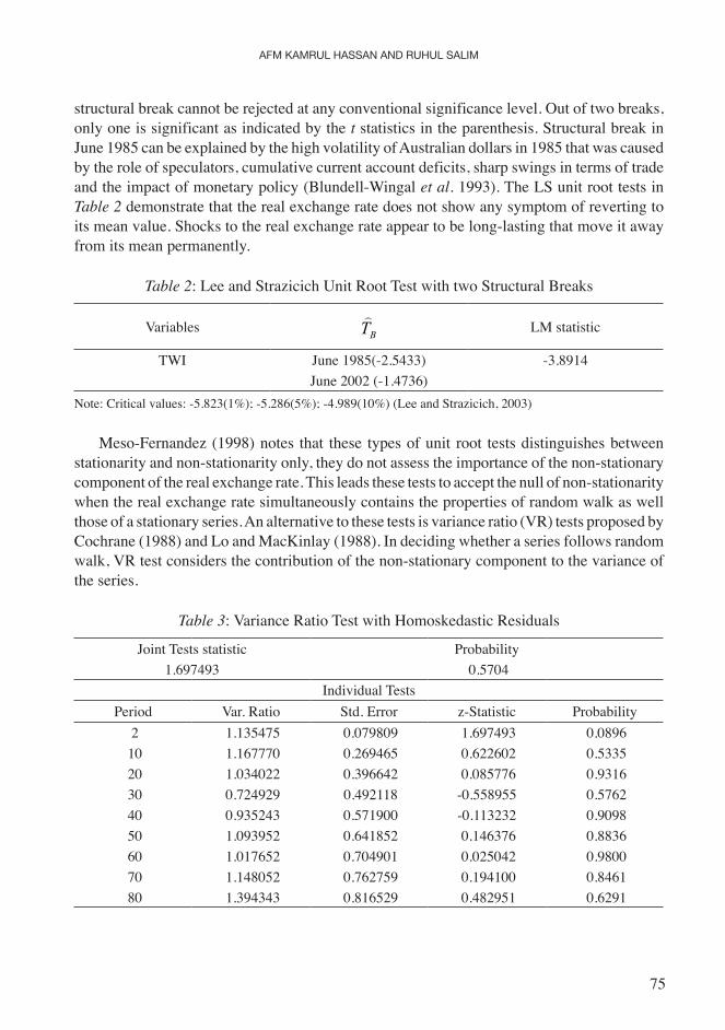
Meso-Fernandez (1998) notes that these types of unit root tests distinguishes between stationarity and non-stationarity only, they do not assess the importance of the non-stationary component of the real exchange rate. This leads these tests to accept the null of non-stationarity when the real exchange rate simultaneously contains the properties of random walk as well those of a stationary series. An alternative to these tests is variance ratio (VR) tests proposed by Cochrane (1988) and Lo and MacKinlay (1988). In deciding whether a series follows random walk, VR test considers the contribution of the non-stationary component to the variance of the series.

Table 3: Variance Ratio Test with Homoskedastic Residuals

Joint Tests statistic Probability1.697493 0.5704

Individual TestsPeriod Var. Ratio Std. Error z-Statistic Probability

2 1.135475 0.079809 1.697493 0.0896 10 1.167770 0.269465 0.622602 0.5335 20 1.034022 0.396642 0.085776 0.9316 30 0.724929 0.492118 -0.558955 0.5762 40 0.935243 0.571900 -0.113232 0.9098 50 1.093952 0.641852 0.146376 0.8836 60 1.017652 0.704901 0.025042 0.9800 70 1.148052 0.762759 0.194100 0.8461 80 1.394343 0.816529 0.482951 0.6291

PurchAsing PowEr PArity (PPP) of AustrAliAn DollAr: Do tEst ProcEDurEs mAttEr?

76

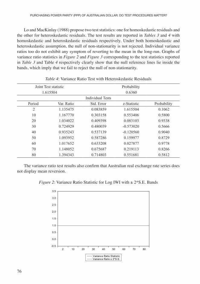
Lo and MacKinlay (1988) propose two test statistics: one for homoskedastic residuals and the other for heteroskedastic residuals. The test results are reported in Tables 3 and 4 with homoskedastic and heteroskedastic residuals respectively. under both homoskedastic and heteroskedastic assumption, the null of non-stationarity is not rejected. Individual variance ratios too do not exhibit any symptom of reverting to the mean in the long-run. Graphs of variance ratio statistics in Figure 2 and Figure 3 corresponding to the test statistics reported in Table 3 and Table 4 respectively clearly show that the null reference lines lie inside the bands, which imply that we fail to reject the null of non-stationarity.

Table 4: Variance Ratio Test with Heteroskedastic Residuals

Joint Test statistic Probability1.615504 0.6360

Individual TestsPeriod Var. Ratio Std. Error z-Statistic Probability

2 1.135475 0.083859 1.615504 0.1062 10 1.167770 0.303158 0.553406 0.5800 20 1.034022 0.409398 0.083103 0.9338 30 0.724929 0.480039 -0.573020 0.5666 40 0.935243 0.537139 -0.120560 0.9040 50 1.093952 0.587286 0.159977 0.8729 60 1.017652 0.633208 0.027877 0.9778 70 1.148052 0.675687 0.219113 0.8266 80 1.394343 0.714803 0.551681 0.5812

The variance ratio test results also confirm that Australian real exchange rate series does not display mean reversion.

Figure 2: Variance Ratio Statistic for Log IWI with ± 2*S.E. Bands

-0.5

0.0

0.5

1.0

1.5

2.0

2.5

3.0

3.5

2 10 20 30 40 50 60 70 80

Variance Ratio StatisticVariance Ratio ± 2*S.E.

Afm KAmrul hAssAn AnD ruhul sAlim

77

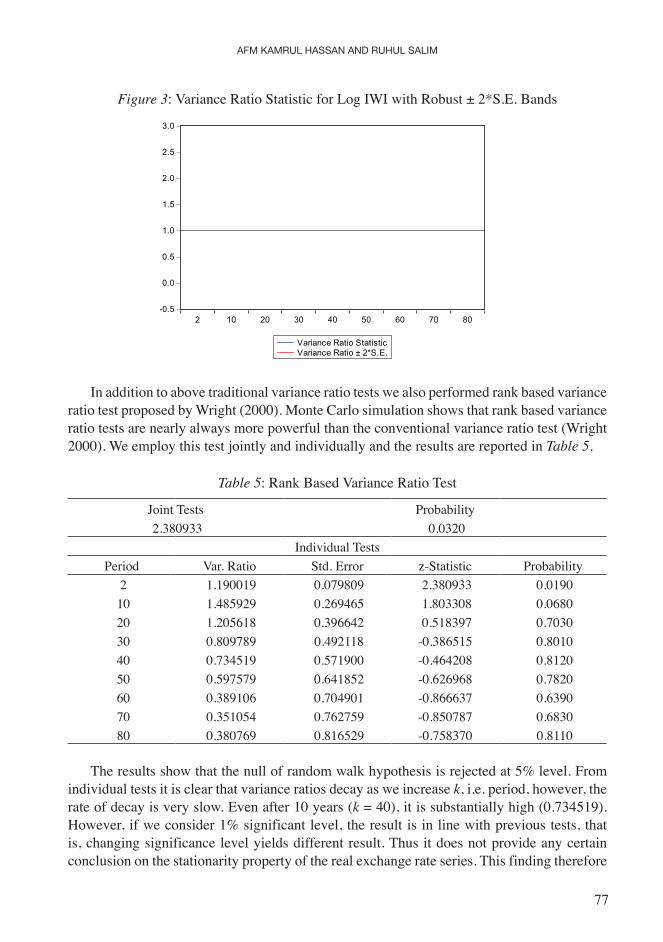
Figure 3: Variance Ratio Statistic for Log IWI with Robust ± 2*S.E. Bands

In addition to above traditional variance ratio tests we also performed rank based variance ratio test proposed by Wright (2000). Monte Carlo simulation shows that rank based variance ratio tests are nearly always more powerful than the conventional variance ratio test (Wright 2000). We employ this test jointly and individually and the results are reported in Table 5.

Table 5: Rank Based Variance Ratio Test

Joint Tests Probability 2.380933 0.0320

Individual TestsPeriod Var. Ratio Std. Error z-Statistic Probability

2 1.190019 0.079809 2.380933 0.0190 10 1.485929 0.269465 1.803308 0.0680 20 1.205618 0.396642 0.518397 0.7030 30 0.809789 0.492118 -0.386515 0.8010 40 0.734519 0.571900 -0.464208 0.8120 50 0.597579 0.641852 -0.626968 0.7820 60 0.389106 0.704901 -0.866637 0.6390 70 0.351054 0.762759 -0.850787 0.6830 80 0.380769 0.816529 -0.758370 0.8110

The results show that the null of random walk hypothesis is rejected at 5% level. From individual tests it is clear that variance ratios decay as we increase k, i.e. period, however, the rate of decay is very slow. Even after 10 years (k = 40), it is substantially high (0.734519). However, if we consider 1% significant level, the result is in line with previous tests, that is, changing significance level yields different result. Thus it does not provide any certain conclusion on the stationarity property of the real exchange rate series. This finding therefore

-0.5

0.0

0.5

1.0

1.5

2.0

2.5

3.0

2 10 20 30 40 50 60 70 80

Variance Ratio StatisticVariance Ratio ± 2*S.E.

PurchAsing PowEr PArity (PPP) of AustrAliAn DollAr: Do tEst ProcEDurEs mAttEr?

78

does not provide strong support to the conventional variance ratio tests and the unit root tests with and without structural breaks.

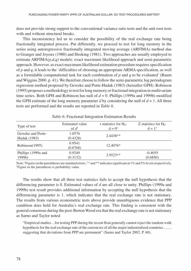
This inconsistency led us to consider the possibility of the real exchange rate being fractionally integrated process. Put differently, we proceed to test for long memory in the series using autoregressive fractionally integrated moving average (ARFIMA) method due to Granger and Joyeux (1980) and Hosking (1981). Two approaches are usually employed to estimate ARFIMA(p,d,q) models: exact maximum likelihood approach and semi-parametric approach. However, as exact maximum likelihood estimation procedure requires specification of p and q, it leads to the ‘difficulties of choosing an appropriate ARMA specification, as well as a formidable computational task for each combination of p and q to be evaluated’ (Baum and Wiggins 2000, p. 41). We therefore choose to follow the semi-parametric log periodogram regression method proposed by Geweke and Porte-Hudak (1983) (hereafter GPH). Robinson (1995) proposes a methodology to test for long memory or fractional integration in multivariate time series. Both GPH and Robinson has null of d = 0. Phillips (1999a and 1999b) modified the GPH estimate of the long memory parameter d by considering the null of d = 1. All three tests are performed and the results are reported in Table 6.

Table 6: Fractional Integration Estimation Results

Type of test Estimated value of d1

t statistics for H0: d = 02

Z statistics for H0: d = 13

Geweke and Porte-Hudak (1983)

1.0576(0.4328) 2.4438**

Robinson(1995) 0.9541(0.0768) 12.4076*

Phillips (1999a and 1999b)

0.9249(0.3132) 2.9523** -0.4055

(0.6850)note: 1Figures in the parentheses are standard errors, 2 * and ** indicates significant at 1% and 5% levels respectively. 3Figure in the parenthesis is probability value.

The results show that all three test statistics fails to accept the null hypothesis that the differencing parameter is 0. Estimated values of d are all close to unity. Phillips (1999a and 1999b) test result provides additional information by accepting the null hypothesis that the differencing parameter is 1, which indicates that the real exchange rate is not stationary. The results from various econometric tests above provide unambiguous evidence that PPP condition does hold for Australia’s real exchange rate. This finding is consistent with the general consensus during the post-Breton Wood era that the real exchange rate is not stationary as Sarno and Taylor noted

“Empirical studies…for testing PPP during the recent float generally cannot reject the random walk hypothesis for the real exchange rate of the currencies of all the major industrialized countries…….suggesting that deviations from PPP are permanent” (Sarno and Taylor 2002, P. 60).

Afm KAmrul hAssAn AnD ruhul sAlim

79

IV. COnCLuSIOn

The aim of this paper is to reexamine whether Australia’s real exchange rate is stationary or not. Employing a number of alternative econometric tests with 158 quarterly observations we provide evidence that non-stationarity of Australia’s real exchange rate cannot be rejected. Thus, these results confirm the empirical validity of PPP hypothesis in Australia. These results are contradictory to those of Cuestas and Regis (2008), but conform to those of Darné and Hoarau (2007 and 2008). However, our results are more reliable in the sense that we use the most recent econometric methods as well as updated data. The empirical results also find that Australia’s real exchange rate experiences significant structural break in 1985 when Australia experienced high volatility in its exchange rate. We, therefore, believe that generalizing the case of structural break to nonlinear deterministic trend as in Cuestas and Regis (2008) is practically equivalent to ignore some macroeconomic event(s) having significant impact on the real exchange rate.

REFEREnCES

Blundell-Wignall, A. and R.G. Gregory (1990). Exchange rate policy in advanced commodity-exporting countries: The case of Australia and new Zealand. Working paper no. 83, OECD Economics Department, OECD, France.

Cochrane, J.H. (1988). How big is the random walk in GnP?, Journal of Political Economy. 96: 893-920.Corbae, D. and S. Ouliaris (1991). A test of long-run purchasing power oarity allowing for structural

breaks, The Economic Record. 67: 26-33.Cuestas, J.C. and P.J. Regis (2008). Testing for PPP in Australia: Evidence from unit root test against

nonlinear trend stationarity alternatives, Economics Bulletin. 3: 1-8.Darné, O. and J. Hoarau (2007). Further evidence on mean reversion in the Australian exchange rate,

Bulletin of Economic Research. 59: 383-395.Darné, O. and J. Hoarau (2008). The purchasing power parity in Australia: evidence from unit root test

with structural break, Applied Economics Letters. 15:203-206.DeJong, D.n., J.C. nankervis, n.E. Savin, and C.H. Whiteman (1992). The power problem of unit root

tests in time series with autoregressive errors, Journal of Econometrics. 53:323-343.Elliott, G., T. Rothenberg, and J. Stock (1996). Efficient tests for an autoregressive unit root, Econometrica.

64: 813-836.Ellis, L. (2001). Measuring the real exchange rate: Pitfalls and practicalities. Research discussion paper

no. 2001-04, Reserve Bank of Australia, Sydney.Geweke, J. and S. Porter-Hudak (1983). The estimation and application of long-memory time series

models, Journal of Time Series Analysis. 4: 221-238.Granger, C. and R. Joyeux (1980). An introduction to long-memory time series models and fractional

differencing, Journal of Time Series Analysis. 1: 15-29.Henry, Ó. and n. Olekalns (2002). Does the Australian dollar real exchange rate display mean reversion,

Journal of International Money and Finance. 21: 651-666.Hosking, J. (1981). Fractional differencing, Biometrika. 68: 165-176.Koya, S.n. and D. Orden (1994). Terms of trade and the exchange rates of new Zealand and Australia,

Applied Economics. 26: 451-457.Lee, J. and M.C. Strazicich (2003). Minimum largrange multiplier unit root test with two structural

breaks, The Review of Economics and Statistics. 85: 1082- 1089.Lee, M., M. nziramasanga and S.K. Ahn (2002). The real exchange rate: an alternative approach to the

PPP puzzle, Journal of Policy Modeling. 24: 533-538.

PurchAsing PowEr PArity (PPP) of AustrAliAn DollAr: Do tEst ProcEDurEs mAttEr?

80

Lo, A.W. and A.C. MacKinlay (1988). Stock market prices do not follow random walks: Evidence from a simple specification test, The Review of Financial Studies. 1: 41-66.

Meso-Fernandez, F. (1998). Econometric methods and purchasing power parity: short- and long-run PPP, Applied Economics. 30:1443-1457.

nunes, L.C., P. newbold, and C. Kuan (1997). Testing for unit roots with breaks: Evidence on the great crash and the unit root hypothesis reconsidered, Oxford Bulletin of Economics and Statistics. 59: 435-448.

Olekalns, n. and n. Wilkins (1998). Re-examining the evidence for long-run purchasing power parity, The Economic Record. 74: 54-61.

Perron, P. (1997). Further evidence on breaking trend functions in macroeconomic variables, Journal of Econometrics. 80:355-85.

Phillips, P. C. B. (1999a). Discrete Fourier transforms of fractional processes. unpublished working paper no. 1243, Cowles Foundation for Research in Economics, Yale university. Available on the web: http://cowles.econ.yale.edu/P/cd/d12a/d1243.pdf (Accessed June 29, 2010).

Phillips, P. C. B. (1999b). unit root log periodogram regression. unpublished working paper no. 1244, Cowles Foundation for Research in Economics, Yale university. Available on the web: http://cowles.econ.yale.edu/P/cd/d12a/d1244.pdf (Accessed June 29, 2010).

Reserve Bank of Australia (2009). Available on the web: http://www.rba.gov.au/statistics/xls/real-exchange-rates.xls (Accessed in January 20, 2010).

Robinson, P. M. (1995). Log-periodogram regression of time series with long range dependence, Annals of Statistics. 23: 1048–1072.

Rogoff, K. (1996). The purchasing power parity puzzle, Journal of Economic Literature. 34: 647- 668.Sarno, Lucio and Mark P. Taylor 2002. The economics of exchange rates. Cambridge university press,

Cambridge, uK.Tawadros, G.B. (2002). Purchasing power parity in the long-run: evidence from Australia’s recent float,

Applied Financial Economics. 12: 625-631.Wright, J. H. (2000). Alternative variance ratio tests using ranks and signs, Journal of Business and

Statistics. 18: 1-9.Zivot E. and D.W.K. Andrew (1992). Further evidence on the great crash, the oil price shock, and the

unit-root hypothesis, Journal of Business and Economic Statistics. 10 :251-270.

Afm KAmrul hAssAn AnD ruhul sAlim

81

APPEnDIx

Figure A1: Real Exchange Rate and Terms of Trade Indices: 1972:2 – 2009:4

Figure A2: Plots of Real Exchange Rate Indices: 1970:2 – 2009:3

8010

012

014

016

018

0

Quarters

Trade weighted index Export weighted indexImport weighted index

4060

8010

012

0Te

rms

of tr

ade

8010

012

014

016

018

0Tr

ade

wei

ghte

d re

al e

xcha

nge

rate

Quarters

Trade weighted real exchange rate (left scale)Terms of trade (right scale)