Pumping and population inversion -

Laser amplification

Gustav Lindgren

2015-02-12

Contents

Part I: Laser pumping and population inversion Steady state laser pumping and population inversion 4-level laser 3-level laser Laser gain saturation Upper-level laser Transient rate equations Upper-level laser Three-level laser

Solve rate-equations in steady-state Introduce the upper-level model Solve rate-equations under transients

Atomic transitions

Energy-level diagram of Nd:YAG Simplify into ->

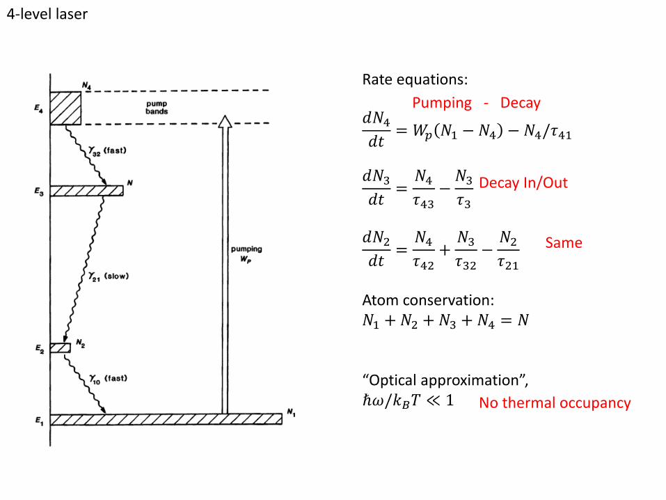
4-level laser

Rate equations: 𝑑𝑁4

𝑑𝑡= 𝑊𝑝 𝑁1 − 𝑁4 − 𝑁4/𝜏41

𝑑𝑁3

𝑑𝑡=

𝑁4

𝜏43−

𝑁3

𝜏3

𝑑𝑁2

𝑑𝑡=

𝑁4

𝜏42+

𝑁3

𝜏32−

𝑁2

𝜏21

Atom conservation: 𝑁1 + 𝑁2 + 𝑁3 + 𝑁4 = 𝑁 “Optical approximation”, ℏ𝜔/𝑘𝐵𝑇 ≪ 1

Pumping - Decay Decay In/Out Same No thermal occupancy

4-level laser

At steady state:

𝑁3 =𝜏3

𝜏43𝑁4

𝑁2 =𝜏21

𝜏32+

𝜏43𝜏21

𝜏42𝜏3𝑁3 ≡ 𝛽𝑁3

For a good laser: 𝛾42≈ 0 (𝑖. 𝑒. 𝜏42 → ∞),

→ 𝛽 ≈𝜏21

𝜏32

Fluorescent quantum efficiency,

𝜂 ≡𝜏4

𝜏43⋅

𝜏3

𝜏𝑟𝑎𝑑

Define beta No direct decay into lev2 → Useful photons: from 4 -> upper laser * From upper laser that lase

4-level laser

Population inversion, 𝑁3 − 𝑁2

𝑁=

1 − 𝛽 𝜂𝑊𝑝𝜏𝑟𝑎𝑑

1 + 1 + 𝛽 +2𝜏43𝜏𝑟𝑎𝑑

𝜂𝑊𝑝𝜏𝑟𝑎𝑑

For a good laser: 𝜏43 ≪ 𝜏𝑟𝑎𝑑 𝛽 ≈ 𝜏21/𝜏32 → 0 𝜂 → 1

⇒𝑁3 − 𝑁2

𝑁≈

𝑊𝑝𝜏𝑟𝑎𝑑

1 + 𝑊𝑝𝜏𝑟𝑎𝑑

- Short lev 4 lifetime - Short lower lev lifetime - High fluorescent quantum efficiency

- Red curves

Calculate the pop. Inv.

3-level laser

𝑑𝑁3

𝑑𝑡= 𝑊𝑝 𝑁1 − 𝑁3 −

𝑁3

𝜏3

𝑁1 + 𝑁2 + 𝑁3 = 𝑁

𝜂 =𝜏3

𝜏32

𝜏21

𝜏𝑟𝑎𝑑

𝛽 =𝑁3

𝑁2=

𝜏32

𝜏21

𝑑𝑁2

𝑑𝑡=

𝑁3

𝜏32−

𝑁2

𝜏21

Rate equations:

Atom conservation:

As before, for 3-level BUT lower level is GROUND level Pumping – decay

decays as before As before Different!

3-level laser

At steady state,

𝑁2 − 𝑁1

𝑁=

1 − 𝛽 𝜂𝑊𝑝𝜏𝑟𝑎𝑑 − 1

1 + 2𝛽 𝜂𝑊𝑝𝜏𝑟𝑎𝑑 + 1

Requirements for pop. inversion: 𝛽 < 1

𝑊𝑝𝜏𝑟𝑎𝑑 ≥1

𝜂 1−𝛽

For a good laser, 𝛽 → 0 𝜂 → 1

𝑁2 − 𝑁1

𝑁≈

𝑊𝑝𝜏𝑟𝑎𝑑 − 1

𝑊𝑝𝜏𝑟𝑎𝑑 + 1

No pumping NEGATIVE pop. Inv. ->

As before New

Red curves

Population inversion

All else equal: 3-level requires more pumping

Upper-level laser

Lasing between two levels high above ground-level 𝑑𝑁3

𝑑𝑡 𝑝𝑢𝑚𝑝= 𝑊𝑝 𝑁0 − 𝑁3

Assuming, 𝑁0 ≈ 𝑁 ≫ 𝑁3 and pump efficiency, 𝜂𝑝, 𝑑𝑁3

𝑑𝑡 𝑝𝑢𝑚𝑝≈ 𝜂𝑝𝑊𝑝𝑁 ≡ 𝑅𝑝

Rate equations: 𝑑𝑁2

𝑑𝑡= 𝑅𝑝 − 𝑊𝑠𝑖𝑔 𝑁2 − 𝑁1 − 𝛾2𝑁2

𝑑𝑁1

𝑑𝑡= 𝑊𝑠𝑖𝑔 𝑁2 − 𝑁1 + 𝛾21𝑁2 − 𝛾1𝑁1

Pump into upper lev. most atoms in ground- state Signal included

Upper-level laser

At steady state:

𝑁1 =𝑊𝑠𝑖𝑔 + 𝛾21

𝑊𝑠𝑖𝑔 𝛾1 + 𝛾20 + 𝛾1𝛾2𝑅𝑝

𝑁2 =𝑊𝑠𝑖𝑔 + 𝛾1

𝑊𝑠𝑖𝑔 𝛾1 + 𝛾20 + 𝛾1𝛾2𝑅𝑝

No atom conservation!

For example, changing pump changes N

Upper-level laser

Population inversion:

Δ𝑁21 = 𝑁2 − 𝑁1 =𝛾1 − 𝛾21

𝛾1𝛾2⋅

𝑅𝑝

1 +𝛾1 + 𝛾20

𝛾1𝛾2𝑊𝑠𝑖𝑔

Define the small-signal population inversion, Δ𝑁0 =𝛾1−𝛾21

𝛾1𝛾2𝑅𝑝 and the effective

recovery time, 𝜏𝑒𝑓𝑓= 𝜏2 1 +𝜏1

𝜏20 the expression becomes:

ΔN21 = Δ𝑁0

1

1 + 𝑊𝑠𝑖𝑔𝜏𝑒𝑓𝑓

For a good laser: 𝛾2 ≈ 𝛾21 𝛾20 ≈ 0

→ ΔN21 ≈ 𝑅𝑝 𝜏2 − 𝜏1 ⋅1

1 + 𝑊𝑠𝑖𝑔𝜏2

The pop. Inv. Saturates as the signal increases

Prop. To pump-rate and lifetimes, saturation behavior

Upper-level laser

• Condition for obtaining inversion, 𝜏1/𝜏21 < 1

i.e. fast relaxation from lower level and slow relaxation from upper level • Small-signal gain,

Δ𝑁0 ∼ 𝑅𝑝 ⋅𝜏2

1 − 𝜏1/𝜏21

i.e. small-signal gain is proportional to the pump-rate times a reduced upper-level lifetime • Saturation behavior,

Δ𝑁21 = Δ𝑁0 ⋅1

1 + 𝑊𝑠𝑖𝑔𝜏𝑒𝑓𝑓

i.e. the saturation intensity depends only on the signal intensity and the effective lifetime, not on the pumping rate.

Upper-level laser: Transient rate equation

Assume: No signal (𝑊𝑠𝑖𝑔 = 0), fast lower-level relaxation (𝑁1 ≈ 0),

𝑑𝑁2 𝑡

𝑑𝑡= 𝑅𝑝 𝑡 − 𝛾2𝑁2 𝑡

The upper level population becomes,

𝑁2 𝑡 = 𝑅𝑝 𝑡′ 𝑒−𝛾2(𝑡−𝑡′)𝑑𝑡′𝑡

−∞

Applying a square pulse,

𝑁2 𝑇𝑝 = 𝑅𝑝0𝜏2(1 − 𝑒−𝑇𝑝/𝜏2)

Define the pump efficiency,

𝜂𝑝 =𝑁2 𝑡 = 𝑇𝑝

𝑅𝑝0𝑇𝑝=

1 − 𝑒−𝑇𝑝/𝜏2

𝑇𝑝/𝜏2

As for instance before a Q-switched pulse

^Pop. In upper lev per pump-photon

3-level laser: pulses

Assume: No signal (𝑊𝑠𝑖𝑔 = 0),

Fast upper-level relaxation (𝜏3 ≈ 0), 𝑑𝑁1

𝑑𝑡= −

𝑑𝑁2

𝑑𝑡≈ −𝑊𝑝 𝑡 𝑁1 𝑡 +

𝑁2 𝑡

𝜏

𝑑

𝑑𝑡Δ𝑁 𝑡 = − 𝑊𝑝 𝑡 +

1

𝜏Δ𝑁 𝑡 + 𝑊𝑝 𝑡 −

1

𝜏𝑁

Square pulse:

Δ𝑁 𝑡

𝑁=

(𝑊𝑝𝜏 − 1) − 2𝑊𝑝 𝜏 ⋅ exp [− 𝑊𝑝𝜏 + 1 𝑡/𝜏]

𝑊𝑝𝜏 + 1

If pump pulse duration is short (𝑇𝑝 ≪ 𝜏),

and the pumping rate is high (𝑊𝑝𝜏 ≫ 1

Δ𝑁 𝑇𝑝𝑁

≈ 1 − 2𝑒−𝑊𝑝𝑇𝑝

3-level laser from prev, no signal

Integrate to get pop. Inv:

Simple model-agrees with experiment!

Summary

Steady state laser pumping and population inversion 4-level laser

𝑁3 − 𝑁2

𝑁≈

𝑊𝑝𝜏𝑟𝑎𝑑

1 + 𝑊𝑝𝜏𝑟𝑎𝑑

3-level laser

𝑁2−𝑁1

𝑁≈

𝑊𝑝𝜏𝑟𝑎𝑑 − 1

1 + 𝑊𝑝𝜏𝑟𝑎𝑑

Laser gain saturation Upper-level laser, saturation behavior

Δ𝑁21 = Δ𝑁0 ⋅1

1+𝑊𝑠𝑖𝑔𝜏𝑒𝑓𝑓

Transient rate equations Upper-level laser

𝜂𝑝 =𝑁2 𝑡 = 𝑇𝑝

𝑅𝑝0𝑇𝑝=

1 − 𝑒−𝑇𝑝/𝜏2

𝑇𝑝/𝜏2

Three-level laser

Δ𝑁 𝑇𝑝

𝑁≈ 1 − 2𝑒−𝑊𝑝𝑇𝑝

Difference between three and four-level systems, and why four-level systems are superior

Saturation intensity is independent of the pumping-rate ”i.e. The signal intensity

needed to reduce the pop. Inv. To half its initial value doesn’t depend on the pumping rate”

Short pulses are needed to obtain high pumping efficiency

These simple models give good agreement with reality

Part II: Laser amplification Wave propagation in atomic media Plane-wave approximation The paraxial wave equation Single-pass laser amplification Gain narrowing Transition cross-sections Gain saturation Power extraction

Contents

Solve wave-eqs See effects on the gain

Wave propagation in an atomic medium

Maxwell’s equations: 𝛻𝑥𝑬 = −𝑗𝜔𝑩 𝛻𝑥𝑯 = 𝑱 + 𝑗𝜔𝑫 Constitutive relations: 𝑩 = 𝜇𝑯 𝑱 = 𝜎𝑬 𝑫 = 𝜖𝑬 + 𝑷𝑎𝑡 = 𝜖 1 + 𝝌𝑎𝑡 𝑬 Vector field of the form:

𝝐 𝒓, 𝑡 =1

2𝑬 𝒓 𝑒𝑗𝜔𝑡 + 𝑐. 𝑐

Assume a spatially uniform material (𝛻 ⋅ 𝐸 = 0), and apply 𝛻 × to get the wave equation:

𝛻2 + 𝜔2𝜇𝜖 1 + 𝜒 𝑎𝑡 −𝑗𝜎

𝜔𝜖𝐸 𝑥, 𝑦, 𝑧 = 0

Material parameters: 𝜇 – magnetic permeability 𝜎 – ohmic losses 𝜖 – dielectric permittivity (not counting atomic transitions) 𝜒𝑎𝑡(𝜔) – resonant susceptibility due to laser transitions

Plane-wave approximation

Consider a plane wave,

𝜕2𝐸

𝜕𝑥2 ,𝜕2𝐸

𝜕𝑦2 ≪𝜕2𝐸

𝜕𝑧2

i.e. 𝛻2 →𝑑2

𝑑𝑧2

The equation reduces to:

𝑑𝑧2 + 𝜔2𝜇𝜖 1 + 𝜒 𝑎𝑡 −

𝑗𝜎

𝜔𝜖𝐸 𝑧 = 0

<- Ok approx. If wavefront is flat

Plane-wave approximation

Without losses: 𝑑𝑧

2 + 𝜔2𝜇𝜖 𝐸 𝑧 = 0, Assume solutions on the form: 𝐸 𝑧 = 𝑐𝑜𝑛𝑠𝑡 ⋅ 𝑒−Γ𝑧

⇒ Γ2 + 𝜔2𝜇𝜖 𝐸 = 0 The allowed values for Γ are, Γ = ±𝑗𝜔 𝜇𝜖 ≡ ±𝑗𝛽 With the solution,

𝝐 𝑧, 𝑡 =1

2𝐸+𝑒𝑗 𝜔𝑡−𝛽𝑧 + 𝐸+

∗𝑒−𝑗 𝜔𝑡−𝛽𝑧 +1

2𝐸−𝑒𝑗 𝜔𝑡+𝛽𝑧 + 𝐸−

∗𝑒−𝑗 𝜔𝑡+𝛽𝑧

The free space propagation constant, 𝛽, may be written:

𝛽 = 𝜔 𝜇𝜖 =𝜔

𝑐=

2𝜋

𝜆

Different beta from last chapter

First, no losses

Plane-wave approximation

With laser action and losses:

𝑑𝑧2 + 𝛽2 1 + 𝜒 𝑎𝑡 −

𝑗𝜎

𝜔𝜖𝐸 𝑧 = 0

Assuming 𝐸 𝑧 = 𝑐𝑜𝑛𝑠𝑡 ⋅ 𝑒−Γ𝑧, as before:

Γ = 𝑗𝛽 1 + 𝜒 𝑎𝑡′ 𝜔 + 𝑗𝜒 𝑎𝑡

′′ 𝜔 − 𝑗𝜎/𝜔𝜖

Normally, 𝜒 𝑎𝑡 𝜔 ,𝜎

𝜔𝜖≪ 1:

Γ ≈ 𝑗𝛽 1 +1

2𝜒𝑎𝑡

′ 𝜔 +𝑗

2 𝜒𝑎𝑡

′′ 𝜔 −𝑗𝜎

2𝜔𝜖=

≡ 𝑗𝛽 + 𝑗Δ𝛽𝑚 𝜔 − 𝛼𝑚 𝜔 + 𝛼0

The final solution becomes:

𝝐 𝑧, 𝑡 = 𝑅𝑒𝐸 0 exp 𝑗𝜔𝑡 − 𝑗 𝛽 + 𝛥𝛽𝑚 𝜔 𝑧 + 𝛼𝑚 𝜔 − 𝛼0 𝑧

1 + 𝛿 ≈ 1 +𝛿

2

Put losses back Expand the sqrt Define four terms

Propagation Factors

𝝐 𝑧, 𝑡 = 𝑅𝑒𝐸 0 exp 𝑗𝜔𝑡 − 𝑗 𝛽 + 𝛥𝛽𝑚 𝜔 𝑧 + 𝛼𝑚 𝜔 − 𝛼0 𝑧 Linear phase-shift (Red) 𝛽 – Plane-wave propagation constant, fundamental phase variation, Nonlinear phase-shift (Blue) Δ𝛽𝑚 𝜔 – Additional atomic phase- shift due to population inversion → Total phase-shift (Green) Gain (Orange) 𝛼𝑚 𝜔 – Atomic gain or loss coefficient (due to transitions) Background 𝛼0 – Ohmic background loss

Phase-shift loss/gain

Exceptions

Larger atomic gain or absorption effects

The results so far are based on the assumption that 𝜒 𝑎𝑡 −𝑗𝜎

𝜔𝜖≪ 1, however, there are a

few situations of interest where this doesn’t hold: - Absorption in metals and semiconductors, at frequencies higher than the bandgap

energy, the effective conductivity, 𝜎 can become very large

- Absorption on strong resonance lines in metal vapor, the transitions are very strongly allowed giving a high absorption per unit length

For expanding the sqrt Big sigma Big chi

The paraxial wave equation

The full wave-equation,

𝛻2 + 𝛽2 1 + 𝜒 𝑎𝑡 −𝑗𝜎

𝜔𝜖𝑬 𝒓 = 0

New ansatz,

𝐸 𝒓 ≡ 𝑢 𝒓 𝑒−𝑗𝛽𝑧 Insert into the wave equation,

𝜕2𝑢

𝜕𝑥2 + 𝜕2𝑢

𝜕𝑦2 +𝜕2𝑢

𝜕𝑧2 − 2𝑗𝛽𝜕𝑢

𝜕𝑧− 𝛽2𝑢 𝑒−𝑗𝛽𝑧 = 0

Assume that 𝑢 𝒓 changes slowly along the z-direction,

𝜕2𝑢

𝜕𝑧2≪ 2𝛽

𝜕𝑢

𝜕𝑧

and 𝜕2𝑢

𝜕𝑧2≪

𝜕2𝑢

𝜕𝑥2,𝜕2𝑢

𝜕𝑦2

⇒ 𝛻𝑡2𝑢 − 2𝑗𝛽

𝜕𝑢

𝜕𝑧+ 𝛽2 𝜒 𝑎𝑡 −

𝑗𝜎

𝜔𝜖𝑢 = 0

Want to handle transverse variations change const -> u(r) ”Paraxial wave equation”

Diffraction- and propagation effects

Rewrite: 𝜕𝑢 𝒓

𝜕𝑧= −

𝑗

2𝛽 𝛻𝑡

2𝑢 𝒓 − [𝛼0−𝛼𝑚 + 𝑗Δ𝛽𝑚]𝑢 𝒓

𝛼0, 𝛼𝑚 𝜔 , and 𝑗Δ𝛽𝑚 𝜔 are defined as before Two terms:

Diffraction, −𝑗

2𝛽 𝛻𝑡

2

Ohmic and atomic gain/loss, −[𝛼0−𝛼𝑚 + 𝑗Δ𝛽𝑚]

Separate terms –> Independent to first order, gain and phase-shift results are the same as for plane waves

Re-write the equation Four terms, same as before Reproduce the plane-wave result

Laser amplification

The laser gain after length L:

𝑔 𝜔 ≡𝐸 𝐿

𝐸 0

In terms of intensity,

𝐺 𝜔 =𝐼 𝐿

𝐼 0=

𝐸 𝐿2

𝐸 02 = exp 2𝛼𝑚 𝜔 𝐿 − 2𝛼0𝐿 = exp [𝛽𝜒′′ 𝜔 𝐿 −

𝜎

𝜖𝑐𝐿]

For most lasers, 𝛼0 ≪ 𝛼𝑚 ⇒ 𝐺 𝜔 ≈ exp (𝛽𝜒′′ 𝜔 𝐿)

Calculate the gain from def. alpha exponential dependence on chi

Gain narrowing

The gain, 𝐺 𝜔 ∼ exp 𝜒′′ 𝜔 → Narrower frequency dependence, i.e. ”Gain Narrowing”

Laser gain & Atomic lineshape FWHM bandwidth is lowered by 30-40%

Absorbing media have opposite sign of 𝜒(𝜔) → ”Absorption broadening”

Absorption broadening

Uninverted population -> absorption broadening

For a black-body: Δ𝑃𝑎𝑏𝑠 = 𝜎 ⋅ 𝐼

Thin slab, atomic densities N1 and N2, cross-sections 𝜎12 and 𝜎21

Net absorbed power: Δ𝑃𝑎𝑏𝑠 = 𝑁1𝜎12 − 𝑁2𝜎21 ⋅ 𝑃Δ𝑧 The cross-sections are related, 𝑔1𝜎12 = 𝑔2𝜎21 Convert power → intensity:

1

𝐼

𝑑𝐼

𝑑𝑧= −Δ𝑁12𝜎21

Previously:

1

𝐼

𝑑𝐼

𝑑𝑧= −2𝛼𝑚(𝜔)

Stimulated transition cross-sections

Loss or gain can be calculated from cross-sections and atomic density

⇒ 2𝛼𝑚 𝜔 = Δ𝑁12𝜎21(𝜔)

Cross-section formula

From previous page: 2𝛼𝑚 𝜔 = Δ𝑁12𝜎21(𝜔)

From definition of 𝛼: 𝛼𝑚 𝜔 =𝜋𝜒′′ 𝜔

𝜆

⇒ 2𝛼𝑚 𝜔 = Δ𝑁𝜎 𝜔 =2𝜋

𝜆 𝜒′′(𝜔)

Using the full expression for 𝜒:

𝜎 𝜔𝑎 =3∗

2𝜋

𝛾𝑟𝑎𝑑

Δ𝜔𝑎𝜆2 ⋅

1

1 + 2(𝜔 − 𝜔𝑎)/Δ𝜔𝑎2

Cross-section estimation: Assume, Δ𝜔𝑎 ≡ 𝛾𝑟𝑎𝑑. (purely radiative transmission), 3 = 3∗, (all atoms aligned)

⇒ 𝜎𝑚𝑎𝑥 =3𝜆2

2𝜋≈

𝜆2

2≈ 10−9𝑐𝑚2

The cross section is far greater than the area of an atom, due to its internal resonance.

The cross-section is a function of wavelength, transition rate and lineshape

Estimate the max cross-section

Real cross-sections

Allowed transitions in gas and non-allowed in solids -> 𝝉𝒈𝒂𝒔 ≪ 𝝉𝒔𝒐𝒍𝒊𝒅

𝜆2

2> Real cross-sections ≫ Atom area

Population difference saturation

Gain saturation, In a medium,

𝑑𝐼

𝑑𝑧= ±2𝛼𝑚𝐼 = ±Δ𝑁𝜎𝐼

As shown previously, Δ𝑁 saturates according to:

Δ𝑁 = Δ𝑁0 ⋅1

1 + 𝑊𝜏𝑒𝑓𝑓= Δ𝑁0 ⋅

1

1 + 𝐼/𝐼𝑠𝑎𝑡

𝑁0 - unsaturated or small signal gain 𝐼𝑠𝑎𝑡 - saturation intensity

Stimulated-transition probability, From before, Δ𝑃𝑎𝑏𝑠 = 𝑁1𝜎12 − 𝑁2𝜎21 ⋅ 𝑃Δ𝑧 From rate equation analysis,Δ𝑃𝑎𝑏𝑠 = 𝑊12𝑁1 − 𝑊21𝑁2 𝐴Δ𝑧ℏ𝜔𝑎

⇒ W =σI

ℏω

i.e. the cross-section, the intensity and the stimulated transition probability are interdependent

As Δ𝑁 saturates, the gain saturates

Population difference saturation

At the line center: From previous slide,

2𝛼𝑚(𝜔, 𝐼) =Δ𝑁0

1 + 𝐼/𝐼𝑠𝑎𝑡=

Δ𝑁0𝜎

1 + 𝜎𝜏𝑒𝑓𝑓/ℏ𝜔 𝐼

→ 𝐼𝑠𝑎𝑡 ≡ℏ𝜔

𝜎𝜏𝑒𝑓𝑓

i.e. 𝐼 = 𝐼𝑠𝑎𝑡: one incident photon within the cross-section per recovery time Off center: The expression is modified by the lineshape,

2𝛼𝑚(𝜔, 𝐼) =Δ𝑁0𝜎

1 +𝐼

𝐼𝑠𝑎𝑡⋅

11 + 𝑦2

Where y is the normalized frequency detuning,

𝑦 = 2 𝜔 − 𝜔0 /Δ𝜔 Frequency dependence due to, transition lineshape and saturation behavior

Re-arrange prev expressions

Practical values

From previous slide,

𝐼𝑠𝑎𝑡 ≡ℏ𝜔

𝜎𝜏𝑒𝑓𝑓

𝐼𝑠𝑎𝑡 is an important parameter since little only little gain will be obtained once the intensity approaches this level. 𝐼𝑠𝑎𝑡 is independent of the pumping intensity, since neither 𝜎 nor 𝜏𝑒𝑓𝑓 are intensity

dependent. However, harder pumping does increase the small-signal gain

Laser type: ℏ𝜔 𝜎 𝜏𝑒𝑓𝑓 𝐼𝑠𝑎𝑡

Gas

10−19 𝐽 10−𝟏𝟑 𝑐𝑚2 10−𝟔 𝑠 1 𝑾/𝑐𝑚2

Solid-state

10−19 𝐽 10−𝟏𝟗 𝑐𝑚2 10−𝟑 𝑠 1 𝒌𝑾/𝑐𝑚2

I-sat varies a lot between materials

Saturation in laser amplifiers

As a signal passes through an amplifier, it grows exponentially with distance until the intensity approaches 𝐼𝑠𝑎𝑡 For a single pass amplifier:

1

𝐼(𝑧)

𝑑𝐼

𝑑𝑧= 2𝛼𝑚 𝐼 =

2𝛼𝑚0

1 + 𝐼(𝑧)/𝐼𝑠𝑎𝑡

Integrating,

1

𝐼+

1

𝐼𝑠𝑎𝑡𝑑𝐼 =

𝐼=𝐼𝑜𝑢𝑡

𝐼=𝐼𝑖𝑛

2𝛼𝑚0 𝑑𝑧

𝑧=𝐿

𝑧=0

gives:

ln𝐼𝑜𝑢𝑡

𝐼𝑖𝑛+

𝐼𝑜𝑢𝑡 − 𝐼𝑖𝑛𝐼𝑠𝑎𝑡

= 2𝛼𝑚0𝐿 = ln 𝐺0

where, 𝐺0 is the small-signal gain

Calculate the saturation

Saturation in laser amplifiers

The total gain,

𝐺 ≡𝐼𝑜𝑢𝑡

𝐼𝑖𝑛= 𝐺0 ⋅ exp(−

𝐼𝑜𝑢𝑡 − 𝐼𝑖𝑛𝐼𝑠𝑎𝑡

)

Is the unsaturated gain, reduced by a factor exponentially dependent on 𝐼𝑜𝑢𝑡 − 𝐼𝑖𝑛

Saturation in laser amplifiers

Plotting the normalized output intensity vs the normalized input intensity, it is clear that the transmission tends to unity as the input intensity is increased -The amplifier becomes transparent.

Extracted Intensities

Output Intensities

Gain starts at G0 and declines towards 0 dB

Power-extraction

Define the extracted intensity,

𝐼𝑒𝑥𝑡𝑟 ≡ 𝐼𝑜𝑢𝑡 − 𝐼𝑖𝑛 = ln𝐺0

𝐺⋅ 𝐼𝑠𝑎𝑡

As the amplifier saturates, 𝐺 → 1,

𝐼𝑎𝑣𝑎𝑖𝑙 = lim𝐺→1

ln𝐺0

𝐺⋅ 𝐼𝑠𝑎𝑡 = ln 𝐺0 ⋅ 𝐼𝑠𝑎𝑡

Using ln 𝐺0 = 2𝛼𝑚0𝐿:

𝐼𝑎𝑣𝑎𝑖𝑙 = 2𝛼𝑚0𝐿 ⋅ 𝐼𝑠𝑎𝑡 = Δ𝑁0𝜎𝐿 ⋅ℏ𝜔

𝜎𝜏𝑒𝑓𝑓

And re-writing: 𝐼𝑎𝑣𝑎𝑖𝑙

𝐿≡

𝑃𝑎𝑣𝑎𝑖𝑙

𝑉=

Δ𝑁0ℏ𝜔

𝜏𝑒𝑓𝑓

i.e. the maximum available power is the total inversion energy, Δ𝑁0ℏ𝜔, once every recovery time, 𝜏𝑒𝑓𝑓

Calculate the extracted power

Power-extraction efficiency

Full power extraction requires complete saturation of the amplifier which gives low small-signal gain. Define the extraction efficiency,

𝜂𝑒𝑥𝑡𝑟 ≡𝐼𝑒𝑥𝑡𝑟

𝐼𝑎𝑣𝑎𝑖𝑙=

ln G0 − ln 𝐺

ln 𝐺0= 1 −

𝐺𝑑𝐵

𝐺0,𝑑𝐵

i.e. there’s a tradeoff between effiency and small-signal gain for single-pass amplifiers.

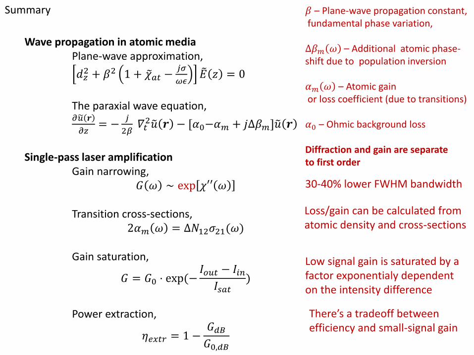
Summary

Wave propagation in atomic media Plane-wave approximation,

𝑑𝑧2 + 𝛽2 1 + 𝜒 𝑎𝑡 −

𝑗𝜎

𝜔𝜖𝐸 𝑧 = 0

The paraxial wave equation,

𝜕𝑢 𝒓

𝜕𝑧= −

𝑗

2𝛽 𝛻𝑡

2𝑢 𝒓 − [𝛼0−𝛼𝑚 + 𝑗Δ𝛽𝑚]𝑢 𝒓

Single-pass laser amplification Gain narrowing,

𝐺 𝜔 ∼ exp 𝜒′′ 𝜔 Transition cross-sections,

2𝛼𝑚 𝜔 = Δ𝑁12𝜎21(𝜔) Gain saturation,

𝐺 = 𝐺0 ⋅ exp(−𝐼𝑜𝑢𝑡 − 𝐼𝑖𝑛

𝐼𝑠𝑎𝑡)

Power extraction,

𝜂𝑒𝑥𝑡𝑟 = 1 −𝐺𝑑𝐵

𝐺0,𝑑𝐵

𝛽 – Plane-wave propagation constant, fundamental phase variation, Δ𝛽𝑚 𝜔 – Additional atomic phase- shift due to population inversion 𝛼𝑚 𝜔 – Atomic gain or loss coefficient (due to transitions) 𝛼0 – Ohmic background loss Diffraction and gain are separate to first order

30-40% lower FWHM bandwidth

Low signal gain is saturated by a factor exponentialy dependent on the intensity difference

Loss/gain can be calculated from atomic density and cross-sections

There’s a tradeoff between efficiency and small-signal gain