puma User Guide

R. D. Pearson, X. Liu, M. Rattray, M. Milo, N. D. LawrenceG. Sanguinetti, Li Zhang

April 30, 2018

Contents

1 Abstract 2

2 Citing puma 2

3 Introduction 3

4 Introductory example analysis - estrogen 54.1 Installing the puma package . . . . . . . . . . . . . . . . . . . . . . . . . 54.2 Loading the package and getting help . . . . . . . . . . . . . . . . . . . . 54.3 Loading in the data . . . . . . . . . . . . . . . . . . . . . . . . . . . . . . 54.4 Determining expression levels for Affymetrix array . . . . . . . . . . . . . 74.5 Determining expression levels for Affymetrix exon arrays . . . . . . . . . 8

4.5.1 gmoExon function . . . . . . . . . . . . . . . . . . . . . . . . . . . 84.5.2 igmoExon function . . . . . . . . . . . . . . . . . . . . . . . . . . 9

4.6 Determining expression levels for Affymetrix hta2.0 arrays . . . . . . . . 104.7 Determining gross differences between arrays . . . . . . . . . . . . . . . . 114.8 Identifying differentially expressed (DE) genes with PPLR method . . . . 144.9 Identifying differentially expressed (DE) genes with IPPLR method . . . 184.10 Clustering with pumaClust . . . . . . . . . . . . . . . . . . . . . . . . . . 204.11 Clustering with pumaClustii . . . . . . . . . . . . . . . . . . . . . . . . . 214.12 Analysis using remapped CDFs . . . . . . . . . . . . . . . . . . . . . . . 21

5 puma for limma users 23

6 Parallel processing with puma 246.1 Parallel processing using socket connections . . . . . . . . . . . . . . . . 24

6.1.1 Parallelisation of pumaComb . . . . . . . . . . . . . . . . . . . . 246.1.2 Parallelisation of gmoExon . . . . . . . . . . . . . . . . . . . . . . 256.1.3 Parallelisation of gmhta . . . . . . . . . . . . . . . . . . . . . . . 26

1

6.2 Parallel processing using MPI . . . . . . . . . . . . . . . . . . . . . . . . 26

7 Session info 27

A Automatic creation of design and contrast matrices 29A.1 Factorial experiments . . . . . . . . . . . . . . . . . . . . . . . . . . . . . 30A.2 Non-factorial designs . . . . . . . . . . . . . . . . . . . . . . . . . . . . . 30A.3 Further help . . . . . . . . . . . . . . . . . . . . . . . . . . . . . . . . . . 30

1 Abstract

Most analyses of Affymetrix GeneChip data (including tranditional 3’ arrays and exonarrays) are based on point estimates of expression levels and ignore the uncertainty ofsuch estimates. By propagating uncertainty to downstream analyses we can improveresults from microarray analyses. For the first time, the puma package makes a suite ofuncertainty propagation methods available to a general audience. In additon to calcultegene expression from Affymetrix 3’ arrays, puma also provides methods to process exonarrays and produces gene and isoform expression for alternative splicing study. puma alsooffers improvements in terms of scope and speed of execution over previously availableuncertainty propagation methods. Included are summarisation, differential expressiondetection, clustering and PCA methods, together with useful plotting functions.

2 Citing puma

The puma package is based on a large body of methodological research. Cit-ing puma in publications will usually involve citing one or more of themethodology papers (1),(2),(3),(4),(5),(6),(7),(8) that the software is based on aswell as citing the software package itself. For the methodology papers, seehttp://www.bioinf.manchester.ac.uk/resources/puma/. puma makes use of the donlp2()function (9) by Peter Spellucci. The use of donlp2() must be acknowledged in any publi-cation which contains results obtained with puma or parts of it. Citation of the author’sname and netlib-source is suitable. The software itself as well as the extension of PPLRto the multi-factorial case (the pumaDE function) can be cited as:

puma: a Bioconductor package for Propagating Uncertainty in Microarray Analysis(2007) Pearson et al. BMC Bioinformatics, 2009, 10:211

The functionalities for processing of exon array data to calculate isoform and geneexpression can be cited as:

puma 3.0: improved uncertainty propagation methods for gene and transcript ex-pression analysis, Liu et al. BMC Bioinformatics, 2013, 14:39.

2

3 Introduction

Microarrays provide a practical method for measuring the expression level of thousandsof genes simultaneously. This technology is associated with many significant sources ofexperimental uncertainty, which must be considered in order to make confident infer-ences from the data. Affymetrix GeneChip arrays have multiple probes associated witheach target. The probe-set can be used to measure the target concentration and thismeasurement is then used in the downstream analysis to achieve the biological aims ofthe experiment, e.g. to detect significant differential expression between conditions, orfor the visualisation, clustering or supervised classification of data.

Most currently popular methods for the probe-level analysis of Affymetrix arrays(e.g. RMA, MAS5.0) only provide a single point estimate that summarises the targetconcentration. Yet the probe-set also contains much useful information about the uncer-tainty associated with this measurement. By using probabilistic methods for probe-levelanalysis it is possible to associate gene expression levels with credibility intervals thatquantify the measurement uncertainty associated with the estimate of target concen-tration within a sample. This within-sample variance is a very significant source ofuncertainty in microarray experiments, especially for relatively weakly expressed genes,and we argue that this information should not be discarded after the probe-level anal-ysis. Indeed, we provide a number of examples were the inclusion of this informationgives improved results on benchmark data sets when compared with more traditionalmethods which do not make use of this information.

PUMA is an acronym for Propagating Uncertainty in Microarray Analysis. Thepuma package is a suite of analysis methods for Affymetrix GeneChip data. It includesfunctions to:

1. Calculate expression levels and confidence measures for those levels from raw CELfile data.

2. Combine uncertainty information from replicate arrays

3. Determine differential expression between conditions, or between more complexcontrasts such as interaction terms

4. Cluster data taking the expression-level uncertainty into account

5. Perform a noise-propagation version of principal components analysis (PCA)

There are a number of other Bioconductor packages which can be used to perform thevarious stages of analysis highlighted above. The affy package gives access to a numberof methods for calculating expression levels from raw CEL file data. The limma packageprovides well-proven methods for determination of differentially expressed genes. Otherpackages give access to clustering and PCA methods. In keeping with the Bioconductorphilosophy, we aim to reuse as much code as possible. In many cases, however, we offer

3

techniques that can be seen as alternatives to techniques available in other packages.Where this is the case, we have attempted to provide tools to enable the user to easilycompare the different methods.

We believe that the best method for learning new techniques is to use them. Assuch, the majority of this user manual (Section 4) is given over to case studies whichhighlight different aspects of the package. The case studies include the scripts requiredto recreate the results shown. At present there is just one case study (based on datafrom the estrogen package), but others will soon be included.

One of the most popular packages within Bioconductor is limma. Because manyusers of the puma package are already likely to be familiar with limma, we have writtena special section (Section 5), highlighting the similarities and differences between thetwo packages. While this section might help experienced limma users get up to speedwith puma more quickly, it is not required reading, particularly for those with little orno experience of limma.

The main benefit of using the propagation of uncertainty in microarray analysis isthe potential of improved end results. However, this improvement does come at the costof increased computational demand, particularly that of the time required to run thevarious algorithms. The key algorithms are, however, parallelisable, and we have builtthis parallel functionality into the package. Users that have access to a computer cluster,or even a number of machines on a network, can make use of this functionality. Detailsof how this should be set up are given in Section 6. This section can be skipped by thosewho will be running puma on a single machine only.

The puma package is intended as a full analysis suite which can be used for all stagesof a typical microarray analysis project. Many users will want to compare differentanalysis methods within R, and the package has been designed with this is mind. Someusers, however, may prefer to carry out some stages of the analysis using tools other thanR. Section 7 gives details on writing out results from key stages of a typical analysis,which can then be read into other software tools.

We have chosen to leave details of individual functions out of this vignette, thoughcomprehensive details can be found in the online help for each function.

This software package uses the optimization program donlp2 (9).

4

4 Introductory example analysis - estrogen

In this section we introduce the main functions of the puma package by applying themto the data from the estrogen package

4.1 Installing the puma package

The recommended way to install puma is to use the biocLite function available fromthe bioconductor website. Installing in this way should ensure that all appropriatedependencies are met.

> source("http://www.bioconductor.org/biocLite.R")

> biocLite("puma")

4.2 Loading the package and getting help

The first step in any puma analysis is to load the package. Start R, and then type thefollowing command:

> library(puma)

To get help on any function, use the help command. For example, to get help onthe pumaDE type one of the following (they are equivalent):

> help(pumaDE)

> ?pumaDE

To see all functions that are available within puma type:

> help(package="puma")

4.3 Loading in the data

To import data using the oligo package,the user must have data at the probe-level.Thismeans that if Affymetrix data are to be imported,the user is expected to have CEL files.

Once sets of such files are available,the user can two tools,depending on the arraymanufacturer,to improt the data:read.celfiles function for CEL files.To assist theuser on obtaining the names of the CEL files,the package providers the list.celfiles

function,which accept the same argrments as the list.files function defined in the Rbase package.The basic usage of the package tools to import CEL files present in thecurrent directory consists in combing the read.files functions with their list.files

function counterparts,as shown below,in a hypothetical example:

5

> library(oligo)

> estrogenFilenames<-list.celfiles()

> oligo.estrogen<-read.celfiles(celFiles)

> pData(oligo.estrogen) <- data.frame(

+ "estrogen"=c("absent","absent","present","present"

+ ,"absent","absent","present","present")

+ , "time.h"=c("10","10","10","10","48","48","48","48")

+ , row.names=rownames(pData(oligo.estrogen))

+ )

When the user use the read.celfiles function to read the CEL files,the oligo pack-age will attempt to identif the annotation package required to read the data in.If this an-notation package is not available on BioConductor,the user should use the pdInfoBuilderpackage to create to create an appropriate annotation.In case oligo fails to identify theannotation package’s name correctly,the user can use the pkgname argument availablefor read.celfiles.

> show(oligo.estrogen)

ExpressionFeatureSet (storageMode: lockedEnvironment)

assayData: 409600 features, 8 samples

element names: exprs

protocolData

rowNames: low10-1.cel low10-2.cel ... high48-2.cel

(8 total)

varLabels: exprs dates

varMetadata: labelDescription channel

phenoData

rowNames: low10-1.cel low10-2.cel ... high48-2.cel

(8 total)

varLabels: index

varMetadata: labelDescription channel

featureData: none

experimentData: use 'experimentData(object)'

Annotation: pd.hg.u95av2

[1] TRUE

Here we can see some information about oligo.estrogen

> pData(oligo.estrogen)

index

low10-1.cel 1

6

low10-2.cel 2

high10-1.cel 3

high10-2.cel 4

low48-1.cel 5

low48-2.cel 6

high48-1.cel 7

high48-2.cel 8

We can see from this phenotype data that this experiment has 2 factors (estrogenand time.h),each of which has two levels (absent vs present, and 10 vs 48), hence this is a2x2 factorial experiment. For each combination of levels we have two replicates,makinga total of 2x2x2 = 8 arrays.

4.4 Determining expression levels for Affymetrix array

We will first use multi-mgMOS to create an expression set object from our raw data.This step is similar to using other summarisation methods such as MAS5.0 or RMA, andfor comparison purposes we will also create an expression set object from our raw datausing RMA. Note that the following lines of code are likely to take a significant amountof time to run, so if you in hurry and you have the pumadata library loaded simply typedata(eset_oligo_mmgmos) and data(eset_oligo_rma) at the command prompt.

> eset_estrogen_mmgmos<-mmgmos(oligo.estrogen,gsnorm="none")

> eset_estrogen_rma<-rma(oligo.estrogen)

Note that we have gsnorm="none" in running mmgmos. The gsnorm option enablesdifferent global scaling (between array) normalizations to be applied to the data. Wehave chosen to use no global scaling normalization here so that we can highlight theneed for such normalization (which we do below). The default option with mmgmos is toprovide a median global scaling normalization, and this is generally recommended.

Unlike many other methods, multi-mgMOS provides information about the expecteduncertainty in the expression level, as well as a point estimate of the expression level.

> exprs(eset_estrogen_mmgmos)[1,]

> assayDataElement(eset_estrogen_mmgmos,"se.exprs")[1,]

Here we can see the expression levels, and standard errors of those expression levels,for the first probe set of the oligo.estrogen data set.

If we want to write out the expression levels and standard errors, to be used elsewhere,this can be done using the write.reslts function.

> write.reslts(eset_estrogen_mmgmos, file="eset_estrogen_mmgmos.rda")

7

This code will create seven different comma-separated value (csv) files inthe working directory. eset_estrogen_exprs.csv will contain expression levels.eset_estrogen_se.csv will contain standard errors. The other files contain differentpercentiles of the posterior distribution, which will only be of interest to expert users.For more details type ?write.reslts at the R prompt.

We also provide a method, PMmmgmos, to calculate gene expression level use PMintensities only. PMmmgmos also return an expression set object.

> eset_estrogen_pmmmgmos <- PMmmgmos(oligo.estrogen,gsnorm="none")

The extraction of expression mean and standard deviation is the same as above.

4.5 Determining expression levels for Affymetrix exon arrays

4.5.1 gmoExon function

We use gmoExon function to calculate gene and transcript expression levels. Firstyou have to install oligo packages for read exon arrays. Second,gmoExon needs touse the relationships between genes, transcripts and probes which we put into puma-data R package. You need to download the latest pumadata package, and type bio-

cLite("pumadata"), library(pumadata) at the R prompt to have it installed.The following scripts use example to show the use of gmoExon function.

> setwd(cel.path) ## go to the directory where you put the CEL files.

> exonFilenames<-c("C0006.CEL","C021.CEL"

+ ,"F023_NEG.CEL","F043_NEG.CEL") ## or you can use exonFilenames<-list.celfiles()

> oligo.exon<-read.celfiles(exonFilenames)

And now we can can use the gmoExon function to calculate the gene and transcriptexpression levels.

> eset_gmoExon<-gmoExon(oligo.exon,exontype="Human",gsnorm="none")

Note that we have exontype=”Human”, gsnorm=”none” in running gmoExon. Theexontype option enables gmoExon to be applied to Human,Mouse and Rat exon arrays.The gsnorm option enables different global scaling (between array) normalizations tobe applied to the data. We have chosen to use no global scaling normalization here sothat we can highlight the need for such normalization (which we do below). The defaultoption with gmoExon is to provide a median global scaling normalization, and this isgenerally recommended.

> exprs(eset_gmoExon$gene)[1,]

> assayDataElement(eset_gmoExon$gene,"se.exprs")[1,]

> exprs(eset_gmoExon$transcript)[1,]

> assayDataElement(eset_gmoExon$transcript,"se.exprs")[1,]

8

Here we can see the gene and transcript expression levels, and standard errors ofthose expression levels, for the first mapped gene and transcripts of the oligo.exon dataset

If we want to write out the expression levels and standard errors, to be used else-where,this can be done using the write.reslts function.

> write.reslts(eset_gmoExon$gene, file="eset_gmoExon_gene")

This code will create seven different comma-separated value (csv) files in the work-ing directory. File eset_gmoExon_gene_exprs.csv will contain gene expression levels.eset_gmoExon_gene_se.csv will contain gene standard errors. The other files containdifferent percentiles of the posterior distribution, which will only be of interest to expertusers. For more details type ?write.reslts at the R prompt.

> write.reslts(eset_gmoExon$transcript, file="eset_gmoExon_transcript")

This code will create seven different comma-separated value (csv) files in the workingdirectory. File eset_gmoExon_transcript_exprs.csv will contain transcript expressionlevels. File eset_gmoExon_transcript_se.csv will contain transcirpt standard errors.The other files contain different percentiles of the posterior distribution, which will onlybe of interest to expert users. For more details type ?write.reslts at the R prompt.

4.5.2 igmoExon function

Besides the gmoExon,we also can use igmoExon to calculate gene and transcript expres-sion levels,which it is effective than gmoExon function.The function requires followinginputs:

cel.path The directory where you put the CEL files.

SampleNameTable It is a tab-separated tablewith two columns,ordered by”Celnames”,”Condition”.For our testing dataset,we can formulate the Sam-pleNameTable like below: Celnames: C006.CEL C021.CEL F023_POS.CEL

FO43_NEG.CEL ; Condition: 1 1 2 2

exontype A string with value be one of ”Human”, ”Mouse”, ”Rat”, specifying the chiptype of the data.

gnsorm The way you want to normalized,and the value is one of ”median”, ”none”,”mean”, ”meanlog”.

condition Yes or No. Choose Yes means the igmoExon function separately calculate thegene expression values by the conditions and than combined the every condition’sresult,and normalized finally.Choose No means the igmoExon calulate the geneexpression values as same as the gmoExon function.

9

Here are the two example as follows:

> cel.path<-"cel.path" ## for example cel.path<-"/home/gao/celData"

> SampleNameTable<-"SampleNameTable"

> eset_igmoExon<-igmoExon(cel.path="cel.path",SampleNameTable="SampleNameTable"

+ , exontype="Human"

+ , gsnorm="none", condition="Yes")

And now we can use the same methods to get the gene and transcript levels by exprsand se.exprs.

4.6 Determining expression levels for Affymetrix hta2.0 arrays

We use gmhta function to calculate gene and transcript expression levels. First you haveto install oligo packages for read hta2.0 arrays. Second,gmhta needs to use the relation-ships between genes, transcripts and probes which we put into pumadata R package.You need to download the latest pumadata package, and type biocLite("pumadata"),library(pumadata) at the R prompt to have it installed.

The following scripts use example to show the use of gmhta function.

> setwd(cel.path) ## go to the directory where you put the CEL files.

> library(puma)

> library(oligo)

> oligo.hta<-read.celfiles(celFiles)

> eset_gmhta<-gmhta(oligo.hta,gsnorm="none")

Note that we have gsnorm=”none” in running gmhta. The gsnorm option enablesdifferent global scaling (between array) normalizations to be applied to the data. Wehave chosen to use no global scaling normalization here so that we can highlight theneed for such normalization (which we do below). The default option with gmhta is toprovide a median global scaling normalization, and this is generally recommended.

> exprs(eset_gmhta$gene)[2,]

> se.exprs(eset_gmhta$gene)[2,]

> exprs(eset_gmhta$transcript)[2,]

> se.exprs(eset_gmhta$transcript)[2,]

Here we can see the gene and transcript expression levels, and standard errors ofthose expression levels, for the first mapped gene and transcripts of the oligo.hta dataset

If we want to write out the expression levels and standard errors, to be used else-where,this can be done using the write.reslts function.

> write.reslts(eset_gmhta$gene, file="eset_gmhta_gene")

10

This code will create seven different comma-separated value (csv) files in the workingdirectory. File eset_gmhta_gene_exprs.csv will contain gene expression levels. Fileeset_gmhta_gene_se.csv will contain gene standard errors. The other files containdifferent percentiles of the posterior distribution, which will only be of interest to expertusers. For more details type ?write.reslts at the R prompt.

> write.reslts(eset_gmhta$transcript, file="eset_gmhta_transcript")

This code will create seven different comma-separated value (csv) files in the workingdirectory. File eset_gmhta_transcript_exprs.csv will contain transcript expressionlevels. File eset_gmhta_transcript_se.csv will contain transcript standard errors.The other files contain different percentiles of the posterior distribution, which will onlybe of interest to expert users. For more details type ?write.reslts at the R prompt.

4.7 Determining gross differences between arrays

A useful first step in any microarray analysis is to look for gross differences betweenarrays. This can give an early indication of whether arrays are grouping according tothe different factors being tested. This can also help to identify outlying arrays, whichmight indicate problems, and might lead an analyst to remove some arrays from furtheranalysis.

Principal components analysis (PCA) is often used for determining such gross dif-ferences. puma has a variant of PCA called Propagating Uncertainty in MicroarrayAnalysis Principal Components Analysis (pumaPCA) which can make use of the un-certainty in the expression levels determined by multi-mgMOS. Again, note that thefollowing example can take some time to run, so to speed things up, simply typedata(pumapca_estrogen) at the R prompt.

> pumapca_estrogen <- pumaPCA(eset_estrogen_mmgmos)

For comparison purposes, we will run standard PCA on the expression set createdusing RMA.

> pca_estrogen <- prcomp(t(exprs(eset_estrogen_rma)))

11

> par(mfrow=c(1,2))

> plot(pumapca_estrogen,legend1pos="right",legend2pos="top",main="pumaPCA")

> plot(

+ pca_estrogen$x

+ , xlab="Component 1"

+ , ylab="Component 2"

+ , pch=unclass(as.factor(pData(eset_estrogen_rma)[,1]))

+ , col=unclass(as.factor(pData(eset_estrogen_rma)[,2]))

+ , main="Standard PCA"

+ )

● ●● ●

−0.6 −0.4 −0.2 0.0 0.2 0.4 0.6

−0.

4−

0.2

0.0

0.1

0.2

0.3

pumaPCA

Component 1

Com

pone

nt 2

●

estrogen

absentpresent

time.h

1048

●

●

●

●

−30 −20 −10 0 10 20 30

−20

−10

010

20

Standard PCA

Component 1

Com

pone

nt 2

Figure 1: First two components after applying pumapca and prcomp to the estrogen

data set processed by multi-mgMOS and RMA respectively.

It can be seen from Figure 1 that the first component appears to be separating thearrays by time, whereas the second component appears to be separating the arrays bypresence or absence of estrogen. Note that grouping of the replicates is much tighterwith multi-mgMOS/pumaPCA. With RMA/PCA, one of the absent.48 arrays appearsto be closer to one of the absent.10 arrays than the other absent.48 array. This is notthe case with multi-mgMOS/pumaPCA.

The results from pumaPCA can be written out to a text (csv) file as follows:

> write.reslts(pumapca_estrogen, file="pumapca_estrogen")

Before carrying out any further analysis, it is generally advisable to check the distri-butions of expression values created by your summarisation method. Like PCA analysis,

12

this can help in identifying problem arrays. It can also inform whether further normal-isation needs to be carried out. One way of determining distributions is by using boxplots.

> par(mfrow=c(1,2))

> boxplot(data.frame(exprs(eset_estrogen_mmgmos)),main="mmgMOS - No norm")

> boxplot(data.frame(exprs(eset_estrogen_rma)),main="Standard RMA")

●●

●●

●●●

●●●●

●

●

●●● ●

●●●●●●●●●●

●

●

●●

●●●●●●●●●●

●

●

●●

●●●●●●●●●●●●

●

●●

●

●●

●●●●

●

●●

●●●●

●

●

●●

●●

●

●

●

●

●

●●

low10.1.cel high10.2.cel high48.1.cel

−15

−10

−5

05

1015

mmgMOS − No norm

●

●

●●●●●●●

●

●

●

●●●

●

●

●●●●

●

●

●●

●●●

●

●●●

●

●

●

●●●●

●●●

●

●

●

●

●●

●●

●●

●●

●●●●

●

●●●

●●

●

●●●●

●●

●●

●●

●●

●

●●●

●

●

●●●

●

●

●●

●●●●

●●

●●

●

●● ●

●

●●●●●●●

●

●

●

●●●

●

●

●

●●●

●

●

●●

●●●

●●

●●●

●

●

●

●

●●●

●●

●

●

●

●

●

●

●

●

●●

●●●●

●●●●●

●●

●

●●

●

●●●●

●●

●●

●

●●

●

●

●●●

●

●

●

●●●

●

●

●●

●●●

●

●●

●●

●

●●

●

●

●●●●●●

●

●

●

●

●

●●●

●●●●

●

●

●●

●●

●●●●

●●●

●

●

●●

●

●●●

●●●

●

●●

●●

●●●

●●

●●

●

●●●●

●●

●

●●

●

●

●●●

●●

●●

●●●

●

●●●●●

●

●●●●

●

●●●

●

●●●●●●

●

●●

●●

●

●●●

●

●●●

●

●

●

●

●

●●

●

●

●●

●●

●

●

●●

●●●●●●

●●●

●

●

●●●●●

●●

●

●

●●

●●

●●●

●●

●●●

●

●

●●●●

●●

●

●●

●

●

●●●

●●

●●

●●●●

●●

●●

●●●

●

●●●●

●●●

●

●●

●●●●●●

●

●●

●

●

●●●●●

●

●

●

●

●●

●

●

●●

●

●

●

●

●●

●●●●●●

●●●

●●

●

●●

●●

●●

●

●●

●●

●

●●●●●●●●

●

●

●●●

●●

●

●

●

●

●●●●

●●

●●

●●

●

●

●●

●●

●●

●

●●●

●●

●●

●●

●●

●

●●

●

●

●●●●

●

●

●

●

●●

●

●

●●

●

●

●●●

●●●●●

●

●●

●

●

●

●●

●●

●●●●

●●

●●

●

●●●●●●

●

●

●●●

●●

●

●

●

●

●●●

●●

●●

●●

●

●

●●●

●

●

●

●●

●●

●●

●●

●●

●

●

●●

●

●●

●●●●

●

●

●●●●

●●

●

●

●

●

●●

●●●●●

●

●

●●●

●●

●

●

●●●●

●

●

●

●●

●●

●●●

●

●●●●

●

●

●

●●

●

●●

●

●●

●

●

●

●

●●●●●

●●

●●●

●●●

●●●●●

●

●●●

●●●●●●

●

●●●

●

●

●

●

●●●●

●

●

●

●●●

●●

●

●●

●

●

●●●

●

●●

●

●●

●

●

●

●●●

●●●●

●●

●●●●●

●●

●

●

●

●

●

●●

●●

●

●

●

●●●●

●

●●

●

●

●

●

●●●

●●

●

●●

●●●●●

●●

●●

●

●●

low10.1.cel high10.2.cel high48.1.cel

46

810

1214

Standard RMA

Figure 2: Box plots for estrogen data set processed by multi-mgMOS and RMA re-spectively.

From Figure 2 we can see that the expression levels of the time=10 arrays are gen-erally lower than those of the time=48 arrays, when summarised using multi-mgMOS.Note that we do not see this with RMA because the quantile normalisation used inRMA will remove such differences. If we intend to look for genes which are differentiallyexpressed between time 10 and 48, we will first need to normalise the mmgmos results.

13

> eset_estrogen_mmgmos_normd <- pumaNormalize(eset_estrogen_mmgmos)

> boxplot(data.frame(exprs(eset_estrogen_mmgmos_normd))

+ , main="mmgMOS - median scaling")

●●

●●

●●●

●●●●

●

●

●●● ●

●●●●●●●●●●

●

●

●●

●●●●●●●●●●

●

●

●●

●●●●●●●●●●●●

●

●●

●

●●

●●●●

●

●●

●●●●

●

●

●●

●●

●

●

●

●

●

●●

low10.1.cel high10.2.cel high48.1.cel

−15

−10

−5

05

10

mmgMOS − median scaling

Figure 3: Box plot for estrogen data set processed by multi-mgMOS and normalisationusing global median scaling.

Figure 3 shows the data after global median scaling normalisation. We can now seethat the distributions of expression levels are similar across arrays. Note that the defaultoption when running mmgmos is to apply a global median scaling normalization, so thisseparate normalization using pumaNormalize will generally not be needed.

4.8 Identifying differentially expressed (DE) genes with PPLRmethod

There are many different methods available for identifying differentially expressed genes.puma incorporates the Probability of Positive Log Ratio (PPLR) method (5). The PPLRmethod can make use of the information about uncertainty in expression levels providedby multi-mgMOS. This proceeds in two stages. Firstly, the expression level informationfrom the different replicates of each condition is combined to give a single expression level(and standard error of this expression level) for each condition. Note that the followingcode can take a long time to run and a new faster version, IPPLR, is now available asdescribed in section 4.9. The end result is available as part of the pumadata package, sothe following line can be replaced with data(eset_estrogen_comb).

> eset_estrogen_comb <- pumaComb(eset_estrogen_mmgmos_normd)

14

Note that because this is a 2 x 2 factorial experiment, there are a number of contraststhat could potentially be of interest. puma will automatically calculate contrasts whichare likely to be of interest for the particular design of your data set. For example, thefollowing command shows which contrasts puma will calculate for this data set

> colnames(createContrastMatrix(eset_estrogen_comb))

[1] "present.10_vs_absent.10"

[2] "absent.48_vs_absent.10"

[3] "present.48_vs_present.10"

[4] "present.48_vs_absent.48"

[5] "estrogen_absent_vs_present"

[6] "time.h_10_vs_48"

[7] "Int__estrogen_absent.present_vs_time.h_10.48"

Here we can see that there are seven contrasts of potential interest. The first fourare simple comparisons of two conditions. The next two are comparisons between thetwo levels of one of the factors. These are often referred to as “main effects”. The finalcontrast is known as an “interaction effect”.

Don’t worry if you are not familiar with factorial experiments and the previous para-graph seems confusing. The techniques of the puma package were originally developedfor simple experiments where two different conditions are compared, and this will prob-ably be how most people will use puma. For such comparisons there will be just onecontrast of interest, namely “condition A vs condition B”.

The results from pumaComb can be written out to a text (csv) file as follows:

> write.reslts(eset_estrogen_comb, file="eset_estrogen_comb")

To identify genes that are differentially expressed between the different conditionsuse the pumaDE function. For the sake of comparison, we will also determine genes thatare differentially expressed using a more well-known method, namely using the limmapackage on results from the RMA algorithm.

> pumaDERes <- pumaDE(eset_estrogen_comb)

> limmaRes <- calculateLimma(eset_estrogen_rma)

The results of these commands are ranked gene lists. If we want to write out thestatistics of differential expression (the PPLR values), and the fold change values, wecan use the write.reslts.

> write.reslts(pumaDERes, file="pumaDERes")

15

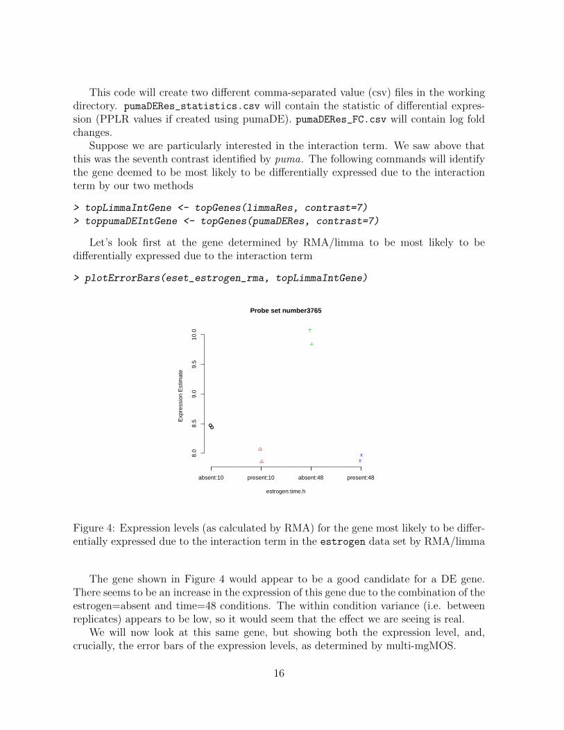
This code will create two different comma-separated value (csv) files in the workingdirectory. pumaDERes_statistics.csv will contain the statistic of differential expres-sion (PPLR values if created using pumaDE). pumaDERes_FC.csv will contain log foldchanges.

Suppose we are particularly interested in the interaction term. We saw above thatthis was the seventh contrast identified by puma. The following commands will identifythe gene deemed to be most likely to be differentially expressed due to the interactionterm by our two methods

> topLimmaIntGene <- topGenes(limmaRes, contrast=7)

> toppumaDEIntGene <- topGenes(pumaDERes, contrast=7)

Let’s look first at the gene determined by RMA/limma to be most likely to bedifferentially expressed due to the interaction term

> plotErrorBars(eset_estrogen_rma, topLimmaIntGene)

●●

estrogen:time.h

Exp

ress

ion

Est

imat

e

absent:10 present:10 absent:48 present:48

8.0

8.5

9.0

9.5

10.0

Probe set number3765

Figure 4: Expression levels (as calculated by RMA) for the gene most likely to be differ-entially expressed due to the interaction term in the estrogen data set by RMA/limma

The gene shown in Figure 4 would appear to be a good candidate for a DE gene.There seems to be an increase in the expression of this gene due to the combination of theestrogen=absent and time=48 conditions. The within condition variance (i.e. betweenreplicates) appears to be low, so it would seem that the effect we are seeing is real.

We will now look at this same gene, but showing both the expression level, and,crucially, the error bars of the expression levels, as determined by multi-mgMOS.

16

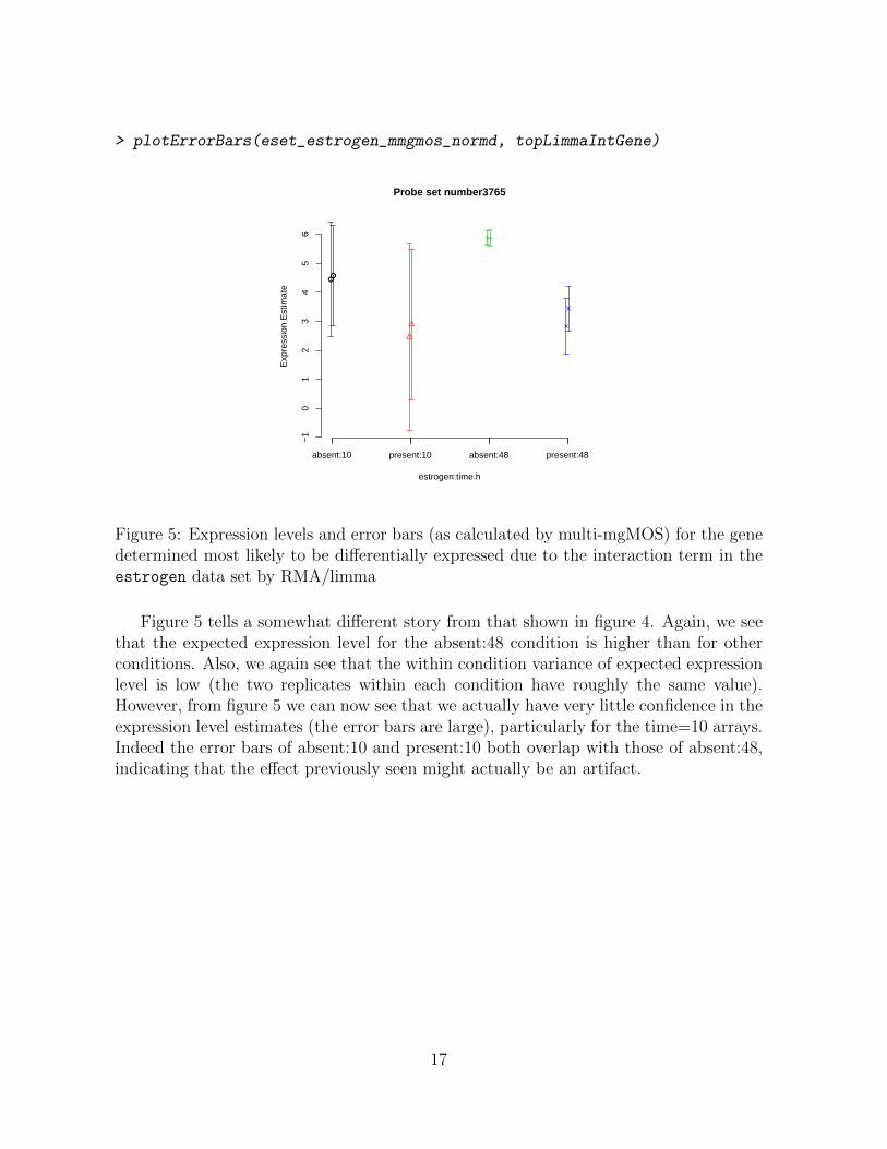
> plotErrorBars(eset_estrogen_mmgmos_normd, topLimmaIntGene)

●●

estrogen:time.h

Exp

ress

ion

Est

imat

e

absent:10 present:10 absent:48 present:48

−1

01

23

45

6

Probe set number3765

Figure 5: Expression levels and error bars (as calculated by multi-mgMOS) for the genedetermined most likely to be differentially expressed due to the interaction term in theestrogen data set by RMA/limma

Figure 5 tells a somewhat different story from that shown in figure 4. Again, we seethat the expected expression level for the absent:48 condition is higher than for otherconditions. Also, we again see that the within condition variance of expected expressionlevel is low (the two replicates within each condition have roughly the same value).However, from figure 5 we can now see that we actually have very little confidence in theexpression level estimates (the error bars are large), particularly for the time=10 arrays.Indeed the error bars of absent:10 and present:10 both overlap with those of absent:48,indicating that the effect previously seen might actually be an artifact.

17

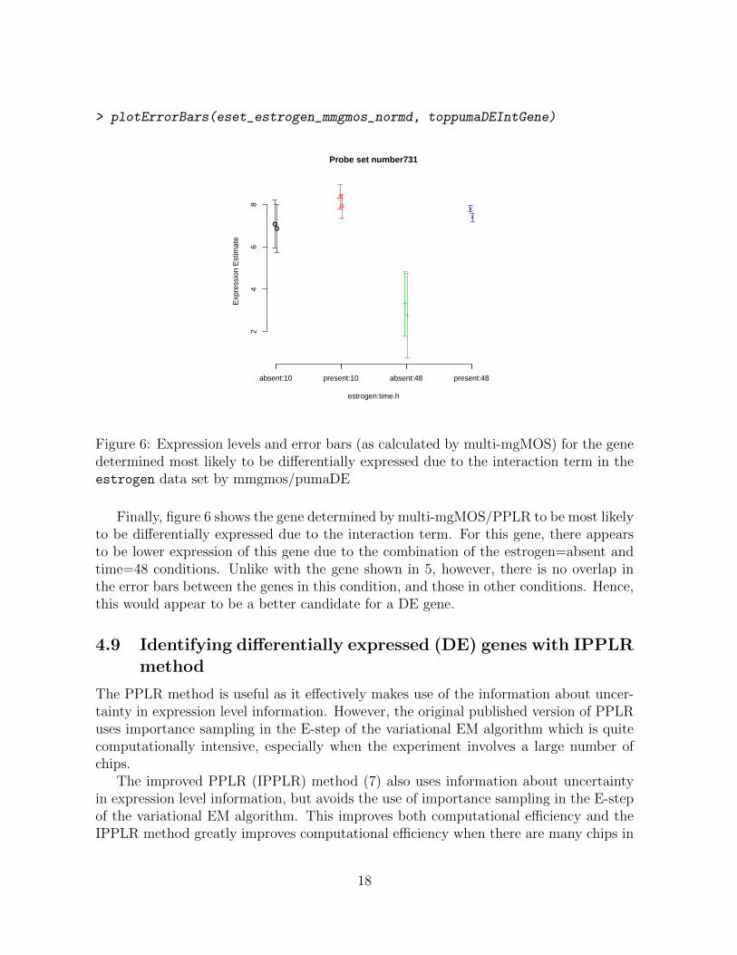
> plotErrorBars(eset_estrogen_mmgmos_normd, toppumaDEIntGene)

●●

estrogen:time.h

Exp

ress

ion

Est

imat

e

absent:10 present:10 absent:48 present:48

24

68

Probe set number731

Figure 6: Expression levels and error bars (as calculated by multi-mgMOS) for the genedetermined most likely to be differentially expressed due to the interaction term in theestrogen data set by mmgmos/pumaDE

Finally, figure 6 shows the gene determined by multi-mgMOS/PPLR to be most likelyto be differentially expressed due to the interaction term. For this gene, there appearsto be lower expression of this gene due to the combination of the estrogen=absent andtime=48 conditions. Unlike with the gene shown in 5, however, there is no overlap inthe error bars between the genes in this condition, and those in other conditions. Hence,this would appear to be a better candidate for a DE gene.

4.9 Identifying differentially expressed (DE) genes with IPPLRmethod

The PPLR method is useful as it effectively makes use of the information about uncer-tainty in expression level information. However, the original published version of PPLRuses importance sampling in the E-step of the variational EM algorithm which is quitecomputationally intensive, especially when the experiment involves a large number ofchips.

The improved PPLR (IPPLR) method (7) also uses information about uncertaintyin expression level information, but avoids the use of importance sampling in the E-stepof the variational EM algorithm. This improves both computational efficiency and theIPPLR method greatly improves computational efficiency when there are many chips in

18

the dataset.The IPPLR method identifies differentially expressed genes in two stages in the same

way as the PPLR method described in Section 4.8. Firstly, the expression level in-formation from the different replicates of each condition is combined to give a singleexpression level (and standard error of this expression level) for each condition. Notethat the following dataset uses the data(eset_mmgmos).

> data(eset_mmgmos)

> eset_mmgmos_100 <- eset_mmgmos[1:100,]

> pumaCombImproved <- pumaCombImproved(eset_mmgmos_100)

pumaComb expected completion time is 9 seconds

.......20%.......40%.......60%.......80%......100%

..................................................

As described for the PPLR method, puma will automatically calculate contrastswhich are likely to be of interst for the particular design of your data set. For example,the following command shows which contrasts puma will calculate for this data set

> colnames(createContrastMatrix(pumaCombImproved))

[1] "20.1_vs_10.1"

[2] "10.2_vs_10.1"

[3] "20.2_vs_20.1"

[4] "20.2_vs_10.2"

[5] "liver_10_vs_20"

[6] "scanner_1_vs_2"

[7] "Int__liver_10.20_vs_scanner_1.2"

From the results, we see that there are seven contrasts of potential interest. The firstfour are simple comparisons of two conditions. The next two are comparisons betweenthe two levels of one of the factors. These are often referred to as “main effects”. Thefinal contrast is known as an “interaction effect”.

The results from the pumaCombImproved can be written out to a text(csv) file asfollows:

> write.reslts(pumaCombImproved,file="eset_mmgmo_combimproved")

The IPPLR method uses the PPLR values to identify the differentially expressedgenes. This process is the same as the PPLR method, so the IPPLR method also usesthe pumaDE.

> pumaDEResImproved <- pumaDE(pumaCombImproved)

19

The results of the command is ranked gene lists. If we want to write out the statisticsof differentiall expression (the PPLR values), and the fold change values, we can use thewrite.reslts.

> write.reslts(pumaDEResImproved,file="pumaDEResImproved")

Section 4.9 gives further examples of how to use the results of this analysis.

4.10 Clustering with pumaClust

The following code will identify seven clusters from the output of mmgmos:

> pumaClust_estrogen <- pumaClust(eset_estrogen_mmgmos, clusters=7)

Clustering is performing ......

Done.

The result of this is a list with different components such as the cluster each probe-set is assigned to and cluster centers. The following code will identify the number ofprobesets in each cluster, the cluster centers, and will write out a csv file with probesetto cluster mappings:

> summary(as.factor(pumaClust_estrogen$cluster))

1 2 3 4 5 6 7

2588 467 1433 157 210 849 6921

> pumaClust_estrogen$centers

low10-1.cel low10-2.cel high10-1.cel high10-2.cel

1 -1.0674686 -0.9938201 -0.73939809 -0.55024065

2 -0.9774309 -0.9450779 -0.09504769 0.05302044

3 -0.9972043 -0.8547680 -0.93359181 -0.60734308

4 -0.8584277 -0.8092580 -1.02476047 -0.81098684

5 -0.9445021 -0.8216593 -0.93525161 -0.56848018

6 -0.6074264 -0.5474843 -1.12535835 -0.86086933

7 -0.9709796 -0.8797100 -0.94108872 -0.72942934

low48-1.cel low48-2.cel high48-1.cel high48-2.cel

1 0.7075239 0.49828214 1.4000784 1.0245430

2 0.2823565 0.06787352 1.4232880 1.1890133

3 0.8574044 0.89406148 0.9982962 1.0991928

4 1.0878300 0.81787879 1.1503577 0.7118062

5 0.9842725 0.96489349 0.8065364 1.1786763

6 1.2465810 1.07918263 0.8309648 0.6065950

7 0.9071089 0.76677990 1.1788024 0.9238939

> write.csv(pumaClust_estrogen$cluster, file="pumaClust_clusters.csv")

20

4.11 Clustering with pumaClustii

The more recently developed pumaClustii method clusters probe-sets taking into ac-count the uncertainties associated with gene expression measurements (from a probe-level analysis model like mgMOS and multi-mmgMOS) but also allowing for replicateinformation. The probabilistic model used is a Student’s t mixture model (8) whichprovides greater robustness than the more standard Gaussian mixture model used bypumaClust (Section 4.10).

The following code will identify six clusters from the output of mmgmos:

> data(Clustii.exampleE)

> data(Clustii.exampleStd)

> r<-vector(mode="integer",0)

> for (i in c(1:20))

+ for (j in c(1:4))

+ r<-c(r,i)

> cl<-pumaClustii(Clustii.exampleE,Clustii.exampleStd,

+ mincls=6,maxcls=6,conds=20,reps=r,eps=1e-3)

Clustering is performing ...

Done.

In this example the vector r contains the labels identifying which experiments shouldbe treated as replicate, and the maxcls and mincls are represented the maximum andminimum number of clusters respectively.

The result of this is a list with different components such as the cluster each probesetis assigned to and cluster centers.You can use the commands described in Section 4.10to obtain information about the results.

4.12 Analysis using remapped CDFs

There is increasing awareness that the original probe-to-probeset mappings provided byAffymetrix are unreliable for various reasons. Various groups have developed alternativeprobe-to-probeset mappings, or“remapped CDFs”, and many of these are available eitheras Bioconductor annotation packages, or as easily downloadable cdf packages.

Importing the CEL files is achieved with the read.celfiles function. The functionwill, in general, correctly identify the annotation package to be used with the experimen-tal data being imported, but the user can specify the pkgname argument to force theuse of a particular one, if for some reason this is required. If the annotation package isnot available from BioConductor, user can use the pdInfoBuilder package to build one.

If you have the ( pd.hg.u95a) and pd.hg.u95b annotation packages, you can do it asfollows:

> oligo.estrogen<-read.celfiles(celFiles,pkgname="pd.hg.u95a")

21

One of the issues with using remapped CDFs is that many probesets in the remappeddata have very few probes. This makes reliable estimation of the expression level of suchprobesets even more problematic than with the original mappings. Because of this, webelieve that even greater attention should be given to the uncertainty in expression levelmeasurements when using remapped CDFs than when using the original mappings. Inthis section we show how to apply the uncertainty propogation methods of puma to there-analysis the estrogen data using a remapped CDF. Note that most of the commandsin this section are the same as the commands in the previous section, showing howstraight-forward it is to do such analysis in puma.

To see the effect of the remapping, the following commands give the numbers ofprobes per probeset using the original, and the remapped CDFs:

> table(table(oligo::probeNames(oligo.estrogen)))

6 7 8 9 10 11 12 13 14 15

8 3 3 4 1 4 11 53 45 39

16 20 69

12387 66 1

Note that, while for the original mapping the vast majority of probesets have 16probes, for the remapped CDF many probesets have less than 16 probes. With thisparticular CDF, probesets with less than 5 probes have been excluded, but this is notthe same for all remapped CDFs.

Analysis can then proceed essentially as before. In the following we will compare theuse of mmgmos/pumaPCA/pumaDE with that of RMA/PCA/limma.

22

5 puma for limma users

puma and limma both have the same primary goal: to identify differentially expressedgenes. Given that many potential users of puma will already be familiar with limma,we have consciously attempted to incorporate many of the features of limma. Mostimportantly we have made the way models are specified in puma, through the creationof design and contrast matrices, very similar to way this is done in limma. Indeed, ifyou have already created design and contrast matrices in limma, these same matricescan be used as arguments to the pumaComb and pumaDE functions.

One of the big differences between the two packages is the ability to automaticallycreate design and contrast matrices within puma, based on the phenotype data suppliedwith the raw data. We believe that these automatically created matrices will be suf-ficient for the large majority of analyses, including factorial designs with up to threedifferent factors. It is even possible, through the use of the createDesignMatrix andcreateContrastMatrix functions, to automatically create these matrices using puma,but then use them in a limma analysis. More details on the automatic creation of designand contrast matrices is given in Appendix A.

One type of analysis that cannot currently be performed within puma, but that isavailable in limma, is the detection of genes which are differentially expressed in at leastone out of three or more different conditions (see e.g. Section 8.6 of the limma usermanual). Factors with more than two levels can be analysed within puma, but only atpresent by doing pairwise comparisons of the different levels. The authors are currentlyworking on extending the functionality of puma to incorporate the detection of genesdifferentially expressed in at least one level of multi-level factors.

puma is currently only applicable to Affymetrix GeneChip arrays, unlike limma,which is applicable to a wide range of arrays. This is due to the calculation of expressionlevel uncertainties within multi-mgMOS from the PM and MM probes which are specificto GeneChip arrays.

23

6 Parallel processing with puma

The most time-consuming step in a typical puma analysis is running the pumaComb

function. This function, however, operates on a probe set by probe set basis, andtherefore it is possible to divide the full set of probe sets into a number of different“chunks”, and process each chunk separately on separate machines, or even on separatecores of a single multi-core machine, hence significantly speeding up the function.

This parallel processing capability has been built in to the puma package, making useof functionality from the R package snow . The snow package itself has been designed torun on the following three underlying technologies: MPI, PVM and socket connections.The puma package has only been tested using MPI and socket connections. We havefound little difference in processing time between these two methods, and currentlyrecommend the use of socket connections as this is easier to set up. Parallel processingin puma has also only been tested to date on a Sun GridEngine cluster. The steps toset up puma on such an architecture using socket connections and MPI are discussed inthe following two sections

6.1 Parallel processing using socket connections

If you do not already have the package snow installed, install this using the followingcommands:

> source("http://bioconductor.org/biocLite.R")

> biocLite("snow")

6.1.1 Parallelisation of pumaComb

To use the parallel functionality of pumaComb you will first need to create a snow“cluster”.This can be done with the following commands. Note that you can have as many nodesin the makeCluster command as you like. You will need to use your own machine namesin the place of “node01”, “node02”, etc. Note you can also use full IP addresses insteadof machine names.

> library(snow)

> cl <- makeCluster(c("node01", "node02", "node03", "node04"), type = "SOCK")

You can then run pumaComb with the created cluster, ensuring the cl parameter isset, as in the following example, which compares the times running on a single node,and running on four nodes:

> library(puma)

> data(affybatch.estrogen)

> pData(affybatch.estrogen) <- data.frame(

24

+ "level"=c("twenty","twenty","ten")

+ , "batch"=c("A","B","A")

+ , row.names=rownames(pData(affybatch.example)))

> eset_mmgmos <- mmgmos(oligo.estrogen)

> system.time(eset_comb_1 <- pumaComb(eset_mmgmos))

> system.time(eset_comb_4 <- pumaComb(eset_mmgmos, cl=cl))

To run pumaComb on multi-cores of a multi-core machine, use a makeCluster com-mand such as the following:

> library(snow)

> cl <- makeCluster(c("localhost", "localhost"), type = "SOCK")

We have found that on a dual-core notebook, the using both cores reduced executiontime by about a third.

Finally, to run on multi-cores of a multi-node cluster, a command such as the follow-ing can be used:

> library(snow)

> cl <- makeCluster(c("node01", "node01", "node02", "node02"

+ , "node03", "node03", "node04", "node04"), type = "SOCK")

6.1.2 Parallelisation of gmoExon

To use the parallel functionality of gmoExon you also need to create a snow“cluster”.Thiscan be done with the following commands:

> library(snow)

> cl<-makeCluster(c("node01","node02","node03","node04"),type = "SOCK")

You can then run gmoExon with the created cluster, as in the following example:

> library(puma)

> library(oligo)

> object<-read.celfiles("filename.CEL")

> eset<-gmoExon(object,exontype="Human",GT="gene",gsnorm="none",cl=cl)

To run gmoExon on multi-core machine, use a makeCluster command such as thefollowing:

> ibrary(snow)

> cl<-makeCluster(c("loaclhost","localhost"),type = "SOCK")

Finally, to run on multi-cores of a multi-node cluster, a command such as the follow-ing can be used:

> library(snow)

> cl<-makeCluster(c("node01","node01","node02" ,"node02"

+ ,"node03" ,"node03" ,"node04" ,"node04"), type = "SOCK")

25

6.1.3 Parallelisation of gmhta

To use the parallel functionality of gmhta you also need to create a snow “cluster”.Thiscan be done with the following commands:

> library(snow)

> cl<-makeCluster(c("node01","node02","node03","node04"),type = "SOCK")

You can then run gmhta with the created cluster, as in the following example:

> library(puma)

> library(oligo)

> object<-read.celfiles("filename.CEL")

> eset<-gmhta(object,gsnorm="none",cl=cl)

To run gmhta on multi-core machine, use a makeCluster command such as the fol-lowing:

> ibrary(snow)

> cl<-makeCluster(c("loaclhost","localhost"),type = "SOCK")

Finally, to run on multi-cores of a multi-node cluster, a command such as the follow-ing can be used:

> library(snow)

> cl<-makeCluster(c("node01","node01","node02" ,"node02"

+ ,"node03" ,"node03" ,"node04" ,"node04"), type = "SOCK")

6.2 Parallel processing using MPI

First follow the steps listed here:

1. Download the latest version of lam-mpi from http://www.lam-mpi.org/

2. Install lam-mpi following the instructions available at http://www.lam-mpi.org/

3. Create a text file called hostfile, the first line of which has the IP address of themaster node of your cluster, and subsequent line of which have the IP addressesof each node you wish to use for processing

4. From the command line type the command lamboot hostfile. If this is successfulyou should see a message saying

LAM 7.1.2/MPI 2 C++/ROMIO - Indiana University

26

(or similar)

5. Install R and the puma package on each node of the cluster (note this will oftensimply involve running R CMD INSTALL on the master node)

6. Install the R packages snow and Rmpi on each node of the cluster

The function pumaComb should automatically run in parallel if the lamboot commandwas successful, and puma , snow and Rmpi are all installed on each node of the cluster.By default the function will use all available nodes.

If you want to override the default parallel behaviour of pumaComb, you can set upyour own cluster which will subsequently be used by the function. This cluster has tobe named cl. To run a cluster with, e.g. four nodes, run the following code:

> library(Rmpi)

> library(snow)

> cl <- makeCluster(4)

> clusterEvalQ(cl, library(puma))

Note that it is important to use the variable name cl to hold the makeCluster

object as puma checks for a variable of this name. The argument to makeCluster (here4) should be the number of nodes on which you want the processing to run (usually thesame as the number of nodes included in the hostfile file, though can also be less).

Running pumaComb in parallel should generally give a speed up almost linear in termsof the number of nodes (e.g. with four nodes you should expect the function to completein about a quarter of the time as if using just one node).

7 Session info

This vignette was created using the following:

> sessionInfo()

R version 3.5.0 (2018-04-23)

Platform: x86_64-pc-linux-gnu (64-bit)

Running under: Ubuntu 16.04.4 LTS

Matrix products: default

BLAS: /home/biocbuild/bbs-3.7-bioc/R/lib/libRblas.so

LAPACK: /home/biocbuild/bbs-3.7-bioc/R/lib/libRlapack.so

locale:

[1] LC_CTYPE=en_US.UTF-8 LC_NUMERIC=C

27

[3] LC_TIME=en_US.UTF-8 LC_COLLATE=C

[5] LC_MONETARY=en_US.UTF-8 LC_MESSAGES=en_US.UTF-8

[7] LC_PAPER=en_US.UTF-8 LC_NAME=C

[9] LC_ADDRESS=C LC_TELEPHONE=C

[11] LC_MEASUREMENT=en_US.UTF-8 LC_IDENTIFICATION=C

attached base packages:

[1] stats4 parallel stats graphics grDevices

[6] utils datasets methods base

other attached packages:

[1] limma_3.36.0 pd.hg.u95av2_3.12.0

[3] DBI_0.8 RSQLite_2.1.0

[5] pumadata_2.15.0 affy_1.58.0

[7] puma_3.22.0 mclust_5.4

[9] oligo_1.44.0 Biostrings_2.48.0

[11] XVector_0.20.0 IRanges_2.14.0

[13] S4Vectors_0.18.0 Biobase_2.40.0

[15] oligoClasses_1.42.0 BiocGenerics_0.26.0

loaded via a namespace (and not attached):

[1] Rcpp_0.12.16 compiler_3.5.0

[3] BiocInstaller_1.30.0 GenomeInfoDb_1.16.0

[5] bitops_1.0-6 iterators_1.0.9

[7] tools_3.5.0 zlibbioc_1.26.0

[9] digest_0.6.15 bit_1.1-12

[11] memoise_1.1.0 preprocessCore_1.42.0

[13] lattice_0.20-35 ff_2.2-13

[15] pkgconfig_2.0.1 Matrix_1.2-14

[17] foreach_1.4.4 DelayedArray_0.6.0

[19] GenomeInfoDbData_1.1.0 affxparser_1.52.0

[21] bit64_0.9-7 grid_3.5.0

[23] BiocParallel_1.14.0 blob_1.1.1

[25] codetools_0.2-15 matrixStats_0.53.1

[27] GenomicRanges_1.32.0 splines_3.5.0

[29] SummarizedExperiment_1.10.0 RCurl_1.95-4.10

[31] affyio_1.50.0

28

A Automatic creation of design and contrast matri-

ces

The puma package has been designed to be as easy to use as possible, while not com-promising on power and flexibility. One of the most difficult tasks for many users,particularly those new to microarray analysis, or statistical analysis in general, is set-ting up design and contrast matrices. The puma package will automatically create suchmatrices, and we believe the way this is done will suffice for most users’ needs.

It is important to recognise that the automatic creation of design and contrastmatrices will only happen if appropriate information about the levels of each factoris available for each array in the experimental design. This data should be held inan AnnotatedDataFrame class. The easiest way of doing this is to ensure that theaffybatch object holding the raw CEL file data has an appropriate phenoData slot.This information will then be passed through to any ExpressionSet object created, forexample through the use of mmgmos. The phenoData slot of an ExpressionSet objectcan also be manipulated directly if necessary.

Design and contrast matrices are dependent on the experimental design. The simplestexperimental designs have just one factor, and hence the phenoData slot will have amatrix with just one column. In this case, each unique value in that column will betreated as a distinct level of the factor, and hence pumaComb will group arrays accordingto these levels. If there are just two levels of the factor, e.g. A and B, the contrastmatrix will also be very simple, with the only contrast of interest being A vs B. Forfactors with more than two levels, a contrast matrix will be created which reflects allpossible combinations of levels. For example, if we have three levels A, B and C, thecontrasts of interest will be A vs B, A vs C and B vs C. In addition, from puma version1.2.1, the following additional contrasts will be created: A vs other (i.e. A vs B & C),B vs other and C vs other.

If we now consider the case of two or more factors, things become more complicated.There are now two cases to be considered: factorial experiments, and non-factorialexperiments. A factorial experiment is one where all the combinations of the levels ofeach factor are tested by at least one array (though ideally we would have a numberof biological replicates for each combination of factor levels). The estrogen case study(Section 4) is an example of a factorial experiment. A non-factorial experiment is onewhere at least one combination of levels is not tested. If we treat the example usedin the puma-package help page as a two-factor experiment (with factors “level” and“batch”), we can see that this is not a factorial experiment as we have no array to testthe conditions “level=ten” and “batch=B”. We will treat the factorial and non-factorialcases separately in the following sections.

29

A.1 Factorial experiments

For factorial experiments, the design matrix will use all columns from the phenoData slot.This will mean that combineRepliactes will group arrays according to a combinationof the levels of all the factors.

A.2 Non-factorial designs

For non-factorial designed experiments, we will simply ignore columns (right to left)from the phenoData slot until we have a factorial design or a single factor. We can seethis in the example used in the puma-package help page. Here we have ignored the“batch” factor, and modelled the experiment as a single-factor experiment (with thatsingle factor being “level”).

A.3 Further help

There are examples of the automated creation of design and contrast matrices for in-creasingly complex experimental designs in the help pages for createDesignMatrix andcreateContrastMatrix.

30

References

[1] Milo M., Niranjan M., Holley M.C., Rattray M., and Lawrence N.D. A probabilisticapproach for summarising oligonucleotide gene expression data. Technical reportavailable upon request, 2005.

[2] Liu X., Milo M., Lawrence N.D., and Rattray M. A tractable probabilistic model foraffymetrix probe-level analysis across multiple chips. Bioinformatics, 21:3637–3644,2005.

[3] Sanguinetti G., Milo M., Rattray M., and Lawrence N.D. Accounting for probe-levelnoise in principal component analysis of microarray data. Bioinformatics, 21:3748–3754, 2005.

[4] Rattray M., Liu X., Sanguinetti G., Milo M., and Lawrence N.D. Propagatinguncertainty in microarray data analysis. Briefings in Bioinformatics, 7:37–47, 2006.

[5] Liu X., Milo M., Lawrence N.D., and Rattray M. Probe-level measurement errorimproves accuracy in detecting differential gene expression. Bioinformatics, 22:2107–2113, 2006.

[6] Liu X., Lin K.K., Andersen B., , and Rattray M. Including probe-level uncertaintyin model-based gene expression clustering. BMC Bioinformatics, 8(98), 2007.

[7] Li Zhang and Xuejun Liu. An improved probabilistic model for finding differentialgene expression. the 2nd BMEI 17–19, oct 2009.

[8] Liu X. and Rattray M. Including probe-level measurement error in robust mixtureclustering of replicated microarray gene expression. Statistical Application in Genet-ics and Molecular Biology., 9(1):Artycle 42, 2010.

[9] Peter Spellucci. Donlp2 code and accompanying documentation. Electronically avail-able via http://plato.la.asu.edu/donlp2.html, 2002.

31