Publishing Community-Preserving Attributed Social Graphs ...

Publishing Community-Preserving Attributed SocialGraphs with a Differential Privacy Guarantee

Xihui Chen1, Sjouke Mauw1,2 and Yunior Ramırez-Cruz1

1SnT, 2CSC, University of Luxembourg

6, av. de la Fonte, L-4364 Esch-sur-Alzette, Luxembourg

{xihui.chen, sjouke.mauw, yunior.ramirez}@uni.lu

September 4, 2019

Abstract

We present a novel method for publishing differentially private synthetic at-tributed graphs. Unlike preceding approaches, our method is able to preserve thecommunity structure of the original graph without sacrificing the ability to cap-ture global structural properties. Our proposal relies on C-AGM, a new community-preserving generative model for attributed graphs. We equip C-AGM with efficientmethods for attributed graph sampling and parameter estimation. For the latter,we introduce differentially private computation methods, which allow us to releasecommunity-preserving synthetic attributed social graphs with a strong formal pri-vacy guarantee. Through comprehensive experiments, we show that our new modeloutperforms its most relevant counterparts in synthesising differentially private at-tributed social graphs that preserve the community structure of the original graph,as well as degree sequences and clustering coefficients.

Keywords: attributed social graphs, generative models, differential privacy, communitydetection

1 Introduction

The use of online social networks (OSNs) has grown steadily during the last years, andis expected to continue growing in the future. Billions of people share many aspects oftheir lives on OSNs and use these systems to interact with each other on a regular basis.The ubiquity of OSNs has turned them into one of the most important sources of data forthe analysis of social phenomena. Such analyses have led to significant findings used ina wide range of applications, from efficient epidemic disease control [22, 5] to informationdiffusion [44, 13].

1

arX

iv:1

909.

0028

0v1

[cs

.SI]

31

Aug

201

9

Despite the undeniable social benefits that can be obtained from social network analysis,access to such data by third parties such as researchers and companies should understand-ably be limited due to the sensitivity of the information stored in OSNs, e.g. personalrelationships, political preferences and religious affiliations. In addition, the increase ofpublic awareness about privacy and the entry into effect of strong privacy regulations suchas GDPR [1] strengthen the reluctance of OSN owners from releasing their data. Therefore,it is of critical importance to provide mechanisms for privacy-preserving data publicationto encourage OSN owners to release data for analysis.

Social graphs are a natural representation of social networks, with nodes correspond-ing to participants and edges to connections between participants. In view of the privacydiscussion, social network owners should only release sanitised sample of the underlyingsocial graphs. However, it has been shown that even social graphs containing only struc-tural information remain vulnerable to privacy attacks leveraging knowledge from publicsources [29], deploying sybil accounts [2, 24], etc. In order to prevent such attacks, a largenumber of graph anonymisation methods have been devised. Initially, the proposed meth-ods focused on editing the original graph via vertex/edge additions and deletions untilobtaining a graph satisfying some privacy property. A critical limitation of graph editingmethods is their reliance on assumptions about the adversary knowledge, which determinethe information that needs to be anonymised and thus the manner in which privacy isenforced. To avoid this type of assumptions, an increasingly popular trend is that of usingsemantic privacy notions, which place formal privacy guarantees on the data processing al-gorithms rather than the dataset. Among semantic privacy notions, differential privacy [8]has become the de facto standard due to its strong privacy guarantees.

According to the type of published data, we can divide differentially private mechanismsfor social graphs into two classes. The methods in the first category directly release specificstatistics of the underlying social graph, e.g. the degree sequence [16, 9] or the numberof specific subgraphs (triangles, stars, etc.) [43]. The second family of methods focuseson publishing synthetic social graphs as a replacement of real social networks in a two-step process [27, 35, 36, 39]. In the first step, differentially private methods are used tocompute the parameters of a generative graph model that accurately captures the originalgraph properties. Then, in the second step, this model is sampled for synthetic graphs,profiting from the fact that the result of post-processing the output of differentially privatealgorithms remains differentially private [17].

Differential privacy requires one to define a privacy budget in advance, which deter-mines the amount of perturbation that will be applied to the outputs of algorithms. Inconsequence, the methods in the first family need to either limit in advance the numberof queries that will be answered or deliver increasingly lower quality answers. On the con-trary, the methods in the second family can devote the entire privacy budget to the modelparameter estimation, without further degradation of the privacy of the sampled graphs.For this reason, in this paper we focus on the second type of methods.

For analysts, the utility of synthetic graphs is determined by the ability of the graphmodels to capture relevant properties of the original graph. To satisfy this need, severalgraph models have been proposed to accurately capture global structural properties such

2

as degree distributions and clustering coefficients, as well as heterogeneous attributes ofthe users such as gender, education or marital status. A common limitation of the afore-mentioned approaches is their inability to represent an important type of information: thecommunity structure. Informally, a community is a set of users who are substantially moreinterrelated among themselves than to other users of the network. This interrelation may,e.g., stem from the explicit existence of relations between the users. An example of sucha community is a group of Gmail users who frequently e-mail each other, as representedby the occurrence of a large number of edges connecting the user nodes from the group.Alternatively, interrelations may stem from the co-occurrence of relevant features, such asusers working at the same company or alumni from the same university. The emergence ofcommunities has been documented to be an inherent property of social networks [34, 41].For analysts, the availability of synthetic attributed graphs that preserve the communitystructure of the original graph represents an opportunity to improve existing applications.For example, they may be able to improve online shopping recommendations based on thecommon purchases of users belonging to the same community. Current models and meth-ods are insufficient for enabling such an analysis, as they either lack information about thecommunity structure or they lack vertex features.

In this paper, we address the problem discussed in the previous paragraph by intro-ducing a new generative attributed graph model, C-AGM (short for Community-PreservingAttributed Graph Model), which in addition to global structural properties, is also capa-ble of preserving the community structure of the original graph. C-AGM is based on theattributed graph model AGM [11], and improves on it by incorporating the capability ofpreserving the number and sizes of the communities of the original graph, as well as thedensities of intra- and inter-community connections (that is, connections between nodesbelonging to the same community or to different communities, respectively). C-AGM alsopreserves a number of statistics describing the correlations between the feature vectors thatdescribe the users and the existence of connections between pairs of users, as well as theircommunity co-affiliation. We equip C-AGM with efficient parameter estimation and graphsampling methods, and provide differentially private variants of the former, which allow usto release synthetic attributed social graphs with a strong privacy guarantee and increasedutility with respect to preceding approaches.

Summary of contributions:

• We propose a new generative attributed graph model, C-AGM, which captures a num-ber of properties of the community structure, as discussed in the previous paragraph,along with global structural properties.

• We present efficient methods for learning an instance of our model from an inputgraph and sampling community-preserving synthetic attributed graphs from this in-stance. We show, via a number of experiments on real-world social networks, that thecommunity structures of synthetic graphs sampled from our model are more similarto those of the original graphs than those of the graphs sampled from previously exist-ing models. Additionally, we show that this behaviour is obtained without sacrificing

3

the ability to preserve global structural features.

• We devise differentially private methods for computing the parameters of the newmodel. We demonstrate that our methods are practical in terms of efficiency andaccuracy. To support the latter claim, we empirically show that differentially privatesynthetic attributed graphs generated by our model suffer a reasonably low degra-dation with respect to their counterparts, in terms of their ability to capture thecommunity structure and structural features of the original graphs.

2 Related Work

Private graph synthesis. The key to synthesising social graphs is the model whichdetermines both the information embedded in the published graphs and the propertiespreserved. Mir et al. [27] used the Kronecker graph generative model [20] to generatedifferentially private graphs. As the Kronecker model cannot accurately capture structuralproperties, Sala et al. [35] proposed an alternative approach which makes use of the dK-graph model. Wang et al. [36] further improved the work of Sala et al. by considering globalsensitivity instead of local sensitivity (refer to Section 3 for the definition of sensitivity).Xiao et al. [39] introduced the HRG-graph model [7] and found that it can further reducethe amount of added noise and thus increase the accuracy.

The approaches described so far work on unlabelled graphs. Pfiffer et al. [11] intro-duced a new model called AGM, which attaches binary attributes to nodes and capturesthe correlations between shared attributes and the existence of connections. Jorgensen etal. [12] adopted this model and proposed differentially private methods to accurately esti-mate the model parameters. They also designed a new graph generation algorithm basedon the TCL model [10], which enables the model to sample attributed graphs preservingthe clustering coefficient. As discussed previously, C-AGM, the model introduced in thispaper, is comparable to this model in preserving global structural properties of the originalgraphs, but it outperforms it by also capturing the community structure.

Private statistics publishing. Degree sequences and degree correlations are two typesof the statistics frequently studied in the literature. The general trend in publishing thesestatistics under differential privacy consists in adding noise to the original sequences andthen post-processing the perturbed sequences to enforce or restore certain properties, suchas graphicality [16], vertex order in terms of degrees [9], etc. Subgraph count queries, e.g.the number of triangles or k-stars, have also received considerable attention. Among theapproaches to accurately compute such queries, we have the so-called ladder functions [43]and smooth sensitivity [15, 37].

Community-preserving graph generation models. A number of existing randomgraph models claim to capture community structure, e.g., BTER [18], ILFR [34], SBM [38]and its variants (e.g., DCSBM [14] and DCPPM [31]). BTER generates community-preservingsocial graphs given expected node degrees and, for every degree value σ, the average of theclustering coefficients of the nodes of degree σ. The model assumes that every community

4

is a set of σ nodes with degree σ. On the contrary, C-AGM makes no assumptions onthe community partition received. Finally, ILFR and the variants of SBM preserve edgedensities at the community level but, unlike our new model, they do not preserve theclustering coefficients of the original graph.

3 Preliminaries

3.1 Notation

An attributed graph is represented as a triple G = (V , E , X), where V = {v1, v2, . . . , vn} isthe set of nodes, E ⊆ V×V is the set of edges, and X is a binary matrix called the attributematrix. The i-th row of X is the attribute vector of vi, which is individually denoted byτ(vi). Every column of X represents a binary feature, which is set to 1 (true), or 0 (false),for each user. For example, if the j-th column represents the attribute “owning a car”,Xij = 1 means that the user represented by vi owns a car. Non-binary real-life attributesare assumed to be binarised. For example, a binarisation of the integer-valued attribute“age” is {“age ≤ 16”, “17 ≤ age ≤ 26”, “27 ≤ age ≤ 64”, “age ≥ 65”}. The orderof the columns of X is fixed, but arbitrary, and has no impact on the results describedhereafter. Throughout the paper, we deal with undirected graphs. That is, if (vi, vj) ∈ E ,then (vj, vi) ∈ E . Additionally, we use A to denote the adjacency matrix of the graph.

We use C = {C0, C1, . . . , Cp}, with Ci ⊆ V for every i ∈ {0, 1, . . . , p}, to representa community partition of the attributed graph. As the term suggests, in this paper weassume that Ci ∩ Cj = ∅, with 0 ≤ i < j ≤ p, and ∪Ci∈CCi = V . The community C0 has aspecial interpretation. Since some community detection algorithms assign no community tosome vertices, we will use C0 as a “discard” community of unassigned vertices. We do so toavoid having a potentially large number of singleton communities, for which no meaningfulco-affiliation statistics can be computed. We use ψC(vi) to denote the community to whichthe node vi belongs in the community partition C. We will use ψ(vi) for short in caseswhere the partition is clear from the context.

3.2 Differential Privacy

Differential privacy [8] is a well studied statistical notion of privacy. The intuition behind itis to randomise the output of an algorithm in such a way that the presence of any individualelement in the input dataset has a negligible impact on the probability of observing anyparticular output. In other words, a mechanism is ε-differentially private if for any pairof neighbouring datasets, i.e. datasets that only differ by one element, the probabilities ofobtaining any output are measurably similar. The amount of similarity is determined bythe parameter ε, which is commonly called the privacy budget. In what follows, we willuse the notation D for the set of possible datasets, O for the set of possible outputs, andD ∼ D′ for a pair of neighbouring datasets.

Definition 1 (ε-differential privacy [8]). A randomised mechanism M : D → O satisfies

5

ε-differential privacy if for every pair of neighbouring datasets D,D′ ∈ D, D ∼ D′, andfor every S ⊆ O, we have

Pr(M(D) ∈ S) ≤ eε Pr(M(D′) ∈ S).

A number of differentially private mechanisms have been proposed. For queries of theform q : D → Rn, the most widely used mechanism to enforce differential privacy is theso-called Laplace mechanism, which consists in obtaining the (non-private) output of q andadding to every component a carefully chosen amount of random noise, which is drawnfrom the Laplace distribution

Lap(λ) : f(y |λ) =1

2λexp(−|y |λ

),

where y is a real-valued variable indicating the noise to be added, λ = ∆q

εand ∆q is a

property of the original function q called global sensitivity. This property is defined as thelargest difference between the outputs of q for any pair of neighbouring datasets, that is

∆q = maxD∼D′

‖q(D)− q(D′)‖1 ,

where ‖·‖1 is the L1 norm. For categorical (non-numerical) queries of the form q : D → O,where O is a finite set of categories, the so-called exponential mechanism [26] is the mostcommonly used. In this case, for each value o ∈ O, a score is assigned by a function(usually called scoring function) quantifying the value’s utility, denoted by u(o,D). Theglobal sensitivity of u is

∆u = maxo∈O,D∼D′

|u(o,D)− u(o,D′)|,

and the randomised output is drawn with probabilityexp(

ε·u(o,D)2∆u

)∑o′∈O exp(

ε·u(o′,D)2∆u

).

Differentially private methods are composable [25]. That is, given a set of algorithms{M1,M2, . . . ,Mn} such that Mi (1 ≤ i ≤ n) satisfies εi-differential privacy, if the al-gorithms are applied sequentially and the results combined by a deterministic method,then the final result satisfies

∑i εi-differential privacy. If the algorithms are applied inde-

pendently on disjoint subsets of the input, then maxi{εi}-differential privacy is satisfied.Moreover, post-processing on the output of an ε-differentially private algorithm also sat-isfies ε-differential privacy if the post-processing is deterministic or randomised with asource of randomness independent from the noise added to the original algorithm [17].These properties allow us to divide a complex computation, such as the set of model pa-rameters in our case, into a sequence of sub-tasks for which differentially private methodsexist or can be more easily developed.

In addition to the global sensitivity, a dataset-dependent notion, called local sensitiv-ity [33], has been enunciated. The local sensitivity of query q on a dataset D is defined as

LS q(D) = maxD∼D′

‖q(D)− q(D′)‖1 ,

that is, the maximum difference between the output of q on D and those on its neighbouringdatasets. It is simple to see that ∆q = maxD LS q(D).

6

4 The C-AGM Model

In this section we give the formal definition of C-AGM. We introduce the methods forsampling synthetic graphs from the model, and describe the methods for learning themodel parameters from an attributed graph.

4.1 Overview

Algorithm 1 summarises the process by which C-AGM is used for publishing syntheticattributed graphs. As discussed in [9, 17, 16], synthetic graph generation is done as apost-processing step of the differentially private computation, so the synthetic graphs arealso differentially private.

Algorithm 1: Given G = (V , E , X), obtain t differentially private attributed syn-thetic graphs.

1 Split privacy budget;2 Obtain differentially private community partition;3 Differentially-privately estimate C-AGM parameters;4 for i ∈ {1, 2, . . . , t} do5 Sample Xi from C-AGM;6 Sample Ei from C-AGM;7 Gi ← (V , Ei, Xi)

8 end

The manner in which the privacy budget is split among the different computations(step 1) is discussed in Section 5. For the differentially private community partition (step 2),we introduce in this paper an extension of the algorithm ModDivisive [32]. The purposeof this extension is to incorporate information from node attributes into the objectivefunction optimised by ModDivisive. We discuss the community partition method in detailin Section 5.1. A thorough description of the parameters of C-AGM is given in Section 4.2,and parameter estimation is discussed in Section 4.4.

Once the model parameters have been estimated, we can sample any number of syn-thetic attributed graphs from the model, as described in steps 4 to 8 of Algorithm 1. Thedifferentially private parameter estimation methods introduced in this paper use the notionof neighbouring attributed graphs [12], which is discussed in detail in the preamble of Sec-tion 5. Under this notion, the existence of relations (edges) and personal characteristicsof the network users (feature vectors) are treated as sensitive, but vertex identities arenot. Thus, the synthetic graphs generated by Algorithm 1 have the same vertex set as theoriginal graph, whereas the attribute matrix and the edge set are sampled from the model(step 7). For every new synthetic attributed graph, we first sample the attribute matrix,and then this matrix is used, in combination with an edge generation model (Section 4.3.1),to generate the edge set of the synthetic graph. There are two reasons for dividing this

7

process into two steps. The first one is to make the sampling process efficient. The secondreason is to profit from the two-step process to enforce the intuition that users with sim-ilar features are more likely to be connected in the social network. The attributed graphsampling procedure is discussed in detail in Section 4.3.

4.2 Model Parameters

As we discussed in Section 1, given an attributed graph G and a community partition Cof G, the purpose of C-AGM is to capture a number of properties of C that are overlookedby previously defined models, without sacrificing the ability to capture global structuralproperties such as degree distributions and clustering coefficients. To that end, C-AGM

models the following properties of the community partition:

1. the number and sizes of communities;

2. the number of intra-community edges in every community;

3. the number of inter-community edges;

4. the distributions of attribute vectors in every community;

5. the distributions of the so-called attribute-edge correlations [12], for the set of inter-community edges and for the set of intra-community edges in every community.

Graphs generated by C-AGM will have the same number of vertices as the original graph,as well as the same number of communities. Moreover, every community will have the samecardinality as in the original graph, and the same number of intra-community edges. Thenumber of inter-community edges of the generated graph will also be the same as that ofthe original graph. Notice that the model preserves the total number, but not necessarilythe pairwise numbers of inter-community edges for every pair of communities.

Attribute-edge correlations were defined in [12] as heuristic values for characterisingthe relation between the feature vectors labelling a pair of vertices and the likelihood thatthese vertices are connected. They encode the intuition that, for example, co-workers whoattended the same university and live near to each other are more likely to be friends thanpersons with fewer features in common, whereas friends are more likely to support thesame sports teams or go to the same bars than unrelated persons. In [12], attribute-edgecorrelations are considered to behave uniformly over the entire graph. Here, we introducethe rationale that they behave differently within different communities, as well as acrosscommunities.

A key element in the representation of attribute-edge correlations is the notion of aggre-gator functions. An aggregator function β : {0, 1}k × {0, 1}k → B maps a pair of attributevectors x, x′ of dimensionality k into a value in a discrete range B, which is used as a de-scriptor, also called aggregated feature, of the pair (x, x′). For example, B can contain a setof similarity levels for pairs of feature vectors, such as {low, medium, high}, and β can map

8

a pair of vectors whose cosine similarity is in the interval [0, 0.33] to low, a pair of vectorswhose cosine similarity is in the interval [0.67, 1] to high, etc. Attribute-edge correlations,along with the community-wise distributions of attribute vectors, are useful for analysts,as they allow to characterise the members of a community in terms of frequently sharedfeatures, hypothesise explanations for the emergence of a community, etc.

Formally, a C-AGM model is defined as a quintuple 〈V , C,ΘcM ,Θ

cX ,Θ

cF 〉, where:

• V is a set of vertices.

• C is a community partition of V .

• ΘcM is an instance of an edge set generative model that preserves properties 1 to 3 of

the community partition C, as well as degree distributions and clustering coefficients.The model introduced in this paper is called CPGM, and is described in detail inSection 4.3.1.

• ΘcX is an instance of an attribute vector generative model, which aims to preserve

property 4. The model defines, for every community C ∈ C and every attributevector x, the probability Pr(τ(v) = x |v ∈ C,Θc

X) that a vertex in Ci is labelled withx. The model introduced in this paper is described in detail in Section 4.4.2.

• ΘcF is an instance of a generative model for attribute-edge correlations, which aims

to preserve property 5. This model defines:

– The discrete range B and an aggregator function β.

– The probability

Pr(β(τ(vi), τ(vj)) = s |ΘcF , ψC(vi) = ψC(vj) = C,Ai,j =1)

for every community C ∈ C and every value s ∈ B.

– The probability

Pr(β(τ(vi), τ(vj)) = s |ΘcF , ψC(vi) 6= ψC(vj), Ai,j =1)

for every value s ∈ B.

The instantiations that we propose for these three components are described in detailin Section 4.4.3.

4.3 Sampling Attributed Graphs from an Instance of C-AGM

Given a C-AGM model G = 〈V , C,ΘcM ,Θ

cX ,Θ

cF 〉, with V = {v1, v2, . . . , vn}, an attributed

graph G = (V , E , X) is sampled from G with probability Pr(G | G) = Pr(E , X | G) which,for the sake of tractability, is approximated as

Pr(E , X |ΘcF ,Θ

cX , C,Θc

M) = Pr(E |ΘcF ,Θ

cM , X, C) · Pr(X |Θc

X , C).

9

That is, we first sample from ΘcX the attribute vectors labelling each vertex and then use

them in sampling the edge set. Again, to keep the sampling process tractable, we introducean additional independence assumption, according to which

Pr(X |ΘcX , C) =

∏v∈V

Pr(τ(v) |ψC(v)).

The computation of the probabilities of the form Pr(x | ψC(v)) will be discussed in Sect-ion 4.4.2. Introducing the assumption that edges are sampled independently from eachother, the probability of generating E given Θc

F , ΘcM , X, and C is

Pr(E | ΘcF ,Θ

cM , X, C) =

∏vi,vj∈V

Pr(Ai,j |ΘcF ,Θ

cM , β(τ(xi), τ(xj)), C).

As it is inefficient to sample edges directly from this distribution, we adapt the samplingmethod introduced in [11] to account for the computation of community-wise separatedcounts. Thus, edges are drawn from the distribution

Q(i, j) ∝ Q′M(i, j) · Γ(β(τ(vi), τ(vj)), C),

where Q′M(i, j) is the probability that (vi, vj) is drawn from the edge generation modelΘcM , given C, as a candidate edge; while Γ(β(τ(vi), τ(vj)), C) is the probability that it is

accepted by ΘF , given C. We split the computation of Γ(β(τ(vi), τ(vj)), C) into two cases:Γintra(β(τ(vi), τ(vj)), C), for every C ∈ C and every i, j such that ψC(vi) = ψC(vj) = C;and Γinter(β(τ(vi), τ(vj))), for every i, j such that ψC(vi) 6= ψC(vj). Formally, we have

Q′M(i, j) =Pr(Ai,j = 1 | Θc

M , C)∑vp,vq∈V Pr(Ap,q = 1 | Θc

M , C),

Γintra(β(τ(vi), τ(vj)), C) =Rintra(β(τ(vi), τ(vj)), C)

SupR,

and Γinter(β(τ(vi), τ(vj))) =Rinter(β(τ(vi), τ(vj)))

SupR,

where

Rintra(β(τ(vi), τ(vj)), C) =Pr(β(τ(vi), τ(vj)) | Θc

F , ψC(vi) = ψC(vj) = C,Ai,j = 1)

Pr(β(τ(vi), τ(vj)) | ΘcM , ψC(vi) = ψC(vj) = C,Ai,j = 1)

,

Rinter(β(τ(vi), τ(vj))) =Pr(β(τ(vi), τ(vj)) | Θc

F , ψC(vi) 6= ψC(vj), Ai,j = 1)

Pr(β(τ(vi), τ(vj)) | ΘcM , ψC(vi) 6= ψC(vj), Ai,j = 1)

,

and SupR = sup⋃

s∈B,C∈C

(Rintra(s, C) ∪Rinter(s)) .

The computation of Q′M(i, j) will be discussed in Section 4.3.1, whereas that ofΓinter(β(τ(vi), τ(vj))), and every Γintra(β(τ(vi), τ(vj)), C) will be discussed in Section 4.4.3.

10

Algorithm 2 describes the procedure to sample an attributed graph from C-AGM. Themethod first generates the attribute vectors (line 1). Then, it pre-computes the acceptanceprobabilities (lines 2 to 11). In line 3, the call to SampleEdgeSet consists in the sequentialexecution of Algs. 3 and 4, which will be described in detail in Section 4.3.1. Finally, theloop in lines 12 to 20 repeatedly draws candidate edges from the edge generation modeland adds to the graph those that are accepted according to the pre-computed probabilities(lines 17 and 18). The method stops when the required number of edges is added.

Algorithm 2: SampleFromCAGM(V , C,ΘcM ,Θ

cX ,Θ

cF )

1 X ′ ← SampleAttributeVectors(ΘcX);

2 Q′M ← ComputeQM(Θc

M , C);3 E ′ ← SampleEdgeSet(Q′

M );4 for s ∈ B do5 Compute Γinter (s);6 for C ∈ C do7 Compute Γintra(s, C)8 end

9 end10 E ′ ← ∅;11 while |E ′| < |E| do12 (v, w)← SampleEdge(Q′

M );13 s← β(τ(v), τ(w));14 u← Uniform(0, 1);15 if (ψC(v) = ψC(w) ∧ u ≤ Γintra(s, ψC(v)) or (ψC(v) 6= ψC(w) ∧ u ≤ Γinter (s) then16 E ′ ← E ′ ∪ {(v, w)};17 end

18 end19 return X ′, E ′;

4.3.1 Edge generation model

As we discussed in Section 4.2, the component ΘcM of C-AGM is an edge generation model

which preserves several properties of the community partition of the original graph (prop-erties 1 to 3 listed in Section 4.2), in addition to the degree distribution and clusteringcoefficients. We call this model CPGM, and describe it in what follows.

The model takes as input the set of vertices, as well as the expected number of neigh-bours of every vertex v within its community (that is, its intra-community degree, denotedby dintra(v)) and the expected number of neighbours outside its community (that is, theinter-community degree, denoted by dinter(v)). These values are used to enforce the ex-pected densities within every community and between communities. Additionally, adapt-ing to our setting a heuristics introduced in [12], the model also requires the number oftriangles having all vertices in one community (which we call intra-community trianglesand denote by nintra

4 ), as well as the number of triangles spanning more than one commu-nity (inter-community triangles, denoted by ninter

4 ). As shown empirically in [12], synthetic

11

graphs that preserve the number of triangles of the original graph are more likely to ap-proximate the clustering coefficient of the original graph. We adopt this intuition as well,but unlike [12], we separate the counts of intra- and inter-community triangles. As wewill discuss in Section 5, nintra

4 and ninter4 can be efficiently and accurately computed under

differential privacy.According to our model, the edge sampling process consists of two steps. The first

step generates a graph that preserves the intra- and inter-community degrees, but not thenumber of intra- and inter-community triangles. Then, the second step iteratively editsthe original edge set until nintra

4 and ninter4 are enforced.

At the first step, we follow the idea of the CL model [6]. For every pair of vertices v andw satisfying ψC(v) = ψC(w) = C, the intra-community edge (v, w) is added with probability

πintraC (v, w) = dintra (v)dintra (w)

2mintraC

, where mintraC is the original number of intra-community edges

in C. That is, intra-community edges are added with a probability proportional to productof the intra-community degrees of the linked vertices. If ψC(v) 6= ψC(w), then the inter-

community edge (v, w) is added with probability πinter(v, w) = dinter (v)dinter (w)2minter , where minter

is the total number of inter-community edges in the original graph. Algorithm 3 describesthe first step of the generation process.

Algorithm 3: GenInitialEdgeSet(dintra , dinter , C)1 E ← ∅;2 for C ∈ C do3 mintra

C ← 12

∑v∈C dintra(v);

4 m← 0;5 while m ≤ mintra

C do6 (v, w)← Sample(πintra

C );7 if (v, w) /∈ E then8 E ← E ∪ {(v, w)};9 m← m+ 1;

10 end

11 end

12 end

13 minter ← 12

∑v∈V dinter (v);

14 while m ≤∑

C∈C mintraC +minter do

15 (v, w)← Sample(πinter );16 if (v, w) /∈ E then17 E ← E ∪ {(v, w)};18 m← m+ 1 ;

19 end

20 end

At the second step, we use the intuition that the clustering behaviour in social networksstems from the higher likelihood of users with common friends to connect [10], thus creatingtriangles. Algorithm 4 enforces the values of nintra

4 and ninter4 of the original graph on the

graph synthesised by Algorithm 3. In Algorithm 4, we denote by Nintra(v) the set ofneighbours of v in its community, that is Nintra(v) = {w | ψC(v) = ψC(w) ∧ (v, w) ∈ E}.

12

Algorithm 4: GetFinalEdgeSet(dintra , dinter , nintra4 , ninter

4 , C)1 µintra

4 ← CountIntraCommTriangles(E);

2 while µintra4 < nintra4 do

3 Uniformly sample C from C;4 Sample v1 from C with probability dintra(v1)

2mintraC

;

5 Uniformly sample v2 from Nintra(v1);6 Uniformly sample v3 from Nintra(v2);7 if (v1, v3) 6∈ E ∧ v3 6= v1 then8 (v′1, v

′2)← GetOldestIntraCommEdge(E , C);

9 nprevcn ← GetCommonNeighbour(v′1, v′2);

10 E ← E/{(v′1, v′2)};11 nnewcn ← GetCommonNeighbour(v1, v3);12 if nprevcn < nnewcn then13 E ← E ∪ {(v1, v3};14 µintra

4 ← µintra4 − nprevcn + nnewcn ;

15 else16 E ← E ∪ {(v′1, v′2)};17 end

18 end

19 end20 µinter

4 ← CountInterCommTriangles(E);

21 while µinter4 < ninter4 do

22 Sample v1 from V with probability dinter (v1)2minter ;

23 Uniformly sample v2 from Ninter (v1);24 Uniformly sample v3 from Nintra(v2);25 (v′1, v

′2)← GetOldestInterCommEdge(E , C);

26 nprevcn ← GetCommonNeighbour(v′1, v′2);

27 E ← E/{(v′1, v′2)};28 nnewcn ← GetCommonNeighbour(v1, v3);29 if nprevcn < nnewcn then30 E ← E ∪ {(v1, v3)} µinter

4 ← µinter4 − nprevcn + nnewcn ;

31 else32 E ← E ∪ {(v′1, v′2)};33 end

34 end

Likewise, we denote by Ninter(v) the set of neighbours of v in different communities, thatis Ninter(v) = {w | ψC(v) 6= ψC(w) ∧ (v, w) ∈ E}. In Algorithm 4, nintra

4 is enforced firstbecause adding or removing an intra-community edge may change the number of inter-community triangles as well, whereas inter-community triangles can be created withoutmodifying the number of intra-community triangles. At every iteration, we sample a newedge. If replacing the oldest intra-community edge (in terms of the order of creation byAlgorithm 3) with the newly sampled edge causes the number of intra-community trianglesto increase, we make the edge exchange permanent. Otherwise, we do not add the newlysampled edge and set the oldest edge to be the youngest, keeping it in the graph. Theiteration stops when the number of intra-community triangles is greater than or equal to

13

that of the original graph. Then, we proceed to enforce the number of inter-communitytriangles by adding inter-community edges. In this case the idea is to find open “wedges”composed of one intra-community edge (u, v) and one inter-community edge (v, w) suchthat the edge (u,w) has not been added to the graph. This ensures that newly added edgeswill not affect the number of intra-community triangles. Let (v′, w′) be the oldest inter-community edge. If the graph obtained by removing (v′, w′) and adding (v, w) containsmore triangles than the current version of the synthetic graph, then (v, w) is added and(v′, w′) is removed. The iteration stops when the number of inter-community triangles isgreater than or equal to that of the original graph.

Due to the removal of initially generated edges, the synthetic graph may become dis-connected. In this case, we apply an edge-swapping post-processing step to reconnect everysmall connected component to the main component (the connected component with themost nodes). If the post-processing reduces the number of triangles, we recall Algorithm 4.The alternation between the post-processing and Algorithm 4 is not guaranteed to yield agraph having exactly the required number of triangles, so we stop the iteration when thetotal number of triangles in the synthetic graph is within a 98% tolerance window withrespect to the original one.

4.4 Parameter Estimation for C-AGM

We now discuss the methods for estimating the parameters of a C-AGM model from a givenattributed graph with a community partition C.

4.4.1 Estimating ΘcM

The estimation of ΘcM reduces to computing the community-wise counters that it relies on:

intra- and inter-community degrees of every vertex, the number of intra-community trian-gles for each community and the number of inter-community triangles. As we mentionedin Section 4.3.1, degrees and triangle counts will be used to preserve global structuralproperties of the generated graphs such as degree distribution and clustering coefficients.They can be efficiently computed in the original graph both exactly and under differentialprivacy.

4.4.2 Estimating ΘcX

In order to keep the estimation procedure tractable, we introduce the assumption thatattributes are independent. This assumption simplifies the estimation and handles thesparsity of the attribute vectors when the number of attributes is large. As seen in [11,12], not having such an assumption severely limits the number of features that can bepractically handled. Furthermore, as we will see in Section 5, in addition to tractability,this assumption will also allow us to limit the amount of noise added by the differentiallyprivate computation.

14

We will denote by x` be the value for the `-th component of the attribute of vector x.Likewise, we will denote by τ`(v) the value of the `-th component of the vector labellingvertex v. We estimate the probability that a node v is labelled with an attribute vector xby the following formula:

Pr(x |v,ΘcX , C) = Pr(x |ψC(v),Θc

X) =k∏`=1

Pr`(x` | ΘcX , ψC(v)),

where k is the number of columns of X (ergo the cardinality of all attribute vectors) and

Pr`(x` | ΘcX , ψC(v)) = |{v′∈ψC(v)|τ`(v′)=x`}|

|ψC(v)| .

4.4.3 Estimating ΘcF

As we discussed in Section 4.2, for defining ΘcF it is necessary to define an aggregator

function for pairs of attribute vectors. Our aggregator function is based on the widelyused cosine similarity, that is, the cosine of the angle between two vectors. Since therange B of aggregator functions needs to be discrete, we split the range [0, 1] of the cosinesimilarity into a set of intervals, determined by a parameter δ satisfying 0 < δ ≤ 1. Letscos(x, x

′) denote the similarity between vectors x and x′. Our aggregator function is

defined as β(x, x′) =⌊scos(x,x′)

δ

⌋. Note that, according to this definition, B = {b s

δc | s ∈

[0, 1]}. Finally, the probability of the attribute vectors of a pair of connected vertices beingdescribed by an aggregated feature u ∈ B is computed as

Pr(β(τ(vi), τ(vj)) = u |ΘcF , C, Ai,j = 1) =

|{(vp,vq)∈E|β(τ(vp),τ(vq))=u∧ψ(vp)=ψ(vq)=ψ(vi)}|

|{(vp,vq)∈E|ψ(vp)=ψ(vq)=ψ(vi)}|

if ψ(vi) = ψ(vj);|{(vp,vq)∈E|β(τ(vp),τ(vq))=u∧ψ(vp)6=ψ(vq)}|

|{(vp,vq)∈E|ψ(vp)6=ψ(vq)|

if ψ(vi) 6= ψ(vj).

Compared to the approach introduced in [11, 12], our method uses a coarser granularityfor aggregated features. Thanks to that, it avoids the need to compute 22k different values,which is not only inefficient, but also results in an excessive amount of noise injected whenapplying differential privacy.

5 Differentially Private C-AGM

In this section, we describe in detail our mechanisms for obtaining differentially privateinstances of the C-AGM model, as well as the necessary adaptations of the sampling methodswhen the model has been computed under differential privacy. As we discussed in Section 3,the difference between different instantiations of differential privacy for graphs lies in thedefinition of the pairs of graphs that are considered to be neighbouring datasets. Here, weadopt the following definition from [12].

15

Definition 2 (Neighbouring attributed graphs [12]). A pair of attributed graphs G =(V , E , X) and G′ = (V , E ′,X ′) are neighbouring, denoted G ∼at G′, if and only if they differin the presence of exactly one edge or the attribute vector of exactly one node. That is,

G ∼at G′ ⇐⇒ |E∇E ′| =1 ∨ (∃v∈V τG(v) 6= τG′(v) ∧ ∀v′∈V\{v} τG(v) = τG′(v)).

Definition 2 entails that the existence of relations, that is the occurrence of edges, andthe attributes describing every particular user, are treated as sensitive. On the contrary,vertex identifiers are treated as non-private. These criteria are in line with the currentprivacy policies of most social networking sites, where the fact that a profile exists ispublic information, but users can keep their personal information and friends list privateor hidden from the general public. With Definition 2 in mind, we describe in what followsthe differentially private computation of every parameter of C-AGM.

5.1 Obtaining the Community Partition

Our differentially private community partition method extends the algorithm ModDivi-sive [32], in such a way that it takes node attributes into account. In its original for-mulation, ModDivisive searches for a community partition that maximises modularity, astructural parameter encoding the intuition that a user tends to be more connected to usersin the same community than to users in other communities [30]. Modularity is defined as

∑C∈C

(`Cm−(dC2m

)2),

where `C is the number of edges between the nodes in C and dC is the sum of degrees of thenodes in C. ModDivisive uses the exponential mechanism, considering the set of possiblepartitions as the categorical co-domain, and using modularity as the scoring function.

In order to integrate node features into ModDivisive, we introduce a new objectivefunction that combines the original modularity with an attribute-based quality criterion.The new objective function is defined as

Q(C) = ws ·Qs(C) + wa ·Qa(C),

where ws ∈ [0, 1], wa = 1−ws, Qs(C) is the modularity of the original graph andQa(C) is themodularity of an auxiliary graph obtained from the original as follows. First, we take thevertex set of the original graph. Then, we compute all pairwise similarities between theirassociated feature vectors. Similarities are computed using the cosine measure (as done inSection 4.4.3 for computing aggregated attributes, but without applying the discretisation).

Finally, we add to the auxiliary graph the edges corresponding to the⌈n(n−1)

20

⌉most similar

attributed node pairs.It is proven in [32] that the global sensitivity of Qs(C) is upper bounded by 3

m, where

m is the minimum number of edges of all potential graphs to publish. In the worst case,

16

∆Qs(C) = 3, considering that the original graph is an arbitrary non-empty graph. However,this is not the case for real-life social graphs, so introducing more realistic assumptionsabout the value of m allows us to use smaller values of ∆Qs(C) and thus reduce the amountof noise added in differentially privately computing Qs(C). Throughout this paper, weassume m = 10, 000, which leads to ∆Qs(C) = 0.0003. As we will see in Section 6, alldatasets used in our experiments comply with this assumption. In what follows, we applyan analogous reasoning for bounding ∆Qa(C).

Proposition 1. Every graph G of order n satisfies LSQa(C)(G) ≤ 60n.

Proof. Let G ∼at G′ be two neighbouring attributed graphs and let Ga and G′a be theauxiliary graphs obtained from G and G′, respectively. If the difference between G and G′

consists only in one edge, then Ga = G′a, so in what follows we will consider that G andG′ differ in one attribute vector. Let v be the (sole) vertex such that τG(v) 6= τG′(v). Inthe worst case, we have that, for every w ∈ V \ {v}, (v, w) ∈ Ga and (v, w) /∈ G′a (or viceversa). It was shown in [32] that the modularities of two graphs differing in one edge differin up to 3

m, where m is the minimum number of edges. Then, in the worst case we have

LSQa(G) ≤ 3(n−1)ma

, where n is the order of G and G′, and ma is the minimum number of

edges in auxiliary graphs. As we discussed in Sect. 5.1, ma ≥ n(n−1)20

, so LSQa(G) ≤ 60n

.The proof is thus completed.

Combining the result in [32] with that of Proposition 1, we conclude that LSQ(C)(G) ≤0.0003 ·ws + 60

|V(G)| ·wa for every G satisfying the aforementioned assumptions, and use thisvalue as an upper bound for ∆Qa(C).

5.2 Attribute Vector Distribution

As discussed in Section 4.4, given a community partition C, in order to obtain the differ-entially private estimation of Θc

X (denoted by Θc

X), we need to compute the probabilitydistribution of each attribute for every community, i.e., Pr`(τ`(v) | Θc

X , v ∈ C), for each` ≤ k (where k is the number of attributes) and C ∈ C. Computing this probability reducesto computing the number of nodes whose `-th attribute has value 1, which we denote by

n`,CX . Let nCX be the sequence(n1,CX , n2,C

X , . . . , nk,CX

). In order to obtain the differentially

private sequence nCX =(n1,CX , n2,C

X , . . . , nk,CX

), we add to each element in nCX noise sampled

from Lap(

kεX

), where εX is the privacy budget reserved for this computation and k is the

global sensitivity of nCX , as shown in the next result.

Proposition 2. The global sensitivity of nCX =(n1,CX , n2,C

X , . . . , nk,CX

)is k.

Proof. Let G ∼at G′ be two neighbouring attributed graphs, let C ⊆ V be a communityand let nCX(G) and nCX(G′) be the instances of nCX in G and G′, respectively. If the differencebetween G and G′ consists only in one edge, then nCX(G) = nCX(G′), so in what follows we

17

will consider that G and G′ differ in one attribute vector. Let v be the (sole) vertex suchthat τG(v) 6= τG′(v). If v /∈ C, then nCX(G) = nCX(G′). On the contrary, if v ∈ C, for everycomponent ` ∈ {1, . . . , k} such that τ`,G(v) 6= τ`,G′(v), we have that

∣∣n`,CX (G)−n`,CX (G′)∣∣ = 1.

In consequence, we have ∆nCX

= maxG∼atG′

∥∥nCX(G)− nCX(G′)∥∥

1= k.

5.3 Attribute-Edge Correlations

Recall that the aggregator function β defined in Section 4.4.3 maps every pair of attributevectors to a non-negative integer in B = {b s

δc | s ∈ [0, 1]}, for some δ ∈ [0, 1]. In order to

estimate ΘcF , we need to count, for each possible output of β, the number of edges whose

end-nodes are mapped to this value. For every t ∈ B and every C ∈ C, let nt,CF be thenumber of intra-community edges (v, v′) in C such that β(τ(v), τ(v′)) = t. Likewise, letn`F inter be the number of inter-community edges (v, v′) such that β(τ(v), τ(v′)) = t. Thus,in order to compute Θ

c

F , we need to differentially privately compute nt,CF for every t ∈ Band every C ∈ C, as well as ntF inter for every t ∈ B. We denote by nt,CF and ntF inter thecorresponding differentially private values.

The global sensitivity of each of these sequences is 2(|V| − 2), which is unbounded.To overcome this problem, we follow an approach analogous to the one used in [12] forcounting attribute-edge correlations in the entire graph. The method, introduced in [3],consists in truncating the edge set of the graph to ensure that the degree of all nodes is atmost p, which in the case of attribute-edge correlations ensures that the global sensitivityis 2p [12, 3]. In consequence, for every C ∈ C, we obtain nt,CF from nt,CF by adding noisesampled from Lap( 2k

εF), where where εF is the privacy budget reserved for this computation.

Likewise, we obtain ntF inter from ntF inter by adding noise sampled from Lap( 2kεF

).

5.4 CPGM Parameters

In what follows we describe the computation of the parameters of CPGM, namely the setof intra-community and inter-community degrees and triangle counts.

Intra- and inter-community degrees. Following the trend of previous differentiallyprivate degree sequence computation methods [16, 9], we first add noise to the raw valuesand then apply a post-processing on the perturbed degree sequences to restore certainproperties of the original sequence, namely graphicality and the order of the nodes interms of their degrees, as well as certain community-specific properties.

Let dCintra = (d1,Cintra , d

2,Cintra . . . , d

m,Cintra), where m = |C| and di,Cintra ≤ di+1,C

intra (1 ≤ i <|C|), be the list of non-decreasingly ordered original intra-community degrees in C ∈C. Analogously, let dCinter = (d1,C

inter , d2,Cinter , . . . , d

m,Cinter) be the sequence of inter-community

degrees of nodes in C.The global sensitivity of the degree sequence of the entire graph is 2, as adding or

removing one edge changes the degrees of exactly two nodes by 1 [9]. The same is true forevery dCintra and dCinter , since the degrees of at most two intra-community nodes (or at mostone node in C and one node outside of C) change by 1. Thus, for every C ∈ C, we obtain

18

from dCintra the differentially private sequence dC by adding noise sampled from Lap( 2εd

) to

every degree value. Similarly, we obtain from dCinter the differentially private sequence di,C

inter .Afterwards, the noisy sequences are post-processed to restore three properties: (i) the non-decreasing order between the intra-community degrees inside every community, (ii) thegraphicality of the intra-community degrees of every community, and (iii) the graphicalityof the inter-community degrees of all nodes in the graph. Property (i) is enforced usingthe method proposed in [9], whereas properties (ii) and (iii) are enforced using the methodproposed in [16].

Numbers of intra- and inter-community triangles. The global sensitivity of thenumber of triangles in a graph is proven in [33] to be n − 2, where n is the number ofvertices. The following result characterises the global sensitivity of the number of intra-community triangles.

Proposition 3. The global sensitivity of the number of intra-community triangles of agraph G with a community partition C is ∆nintra

4= maxC∈C{|C| − 2}.

Proof. Let G ∼at G′ be two neighbouring attributed graphs and let C be a communitypartition of V . Let nintra

4 (G) and nintra4 (G′) be the numbers of intra-community triangles of

G and G′, respectively. If the difference between G and G′ consists only in one attributevector, then nintra

4 (G) = nintra4 (G′), so in what follows we will consider that G and G′ differ

in one edge. We will assume, without loss of generality, that E ′ \ E = (v, v′). Two casesare possible for ψC(v) and ψC(v

′):

(i) ψC(v) 6= ψC(v′). In this case, since (v, v′) is an inter-community edge, nintra

4 (G) =nintra4 (G′).

(ii) ψC(v) = ψC(v′) = C. In this case, we have that nintra

4 (G′)− nintra4 (G) = |C ∩NG(v)∩

NG(v′)|, that is the number of common neighbours of v and v′ in the same community.

It is simple to see that every pair of vertices v and v′ such that ψC(v) = ψC(v′) = C satisfy

|C ∩NG(v) ∩NG(v′)| ≤ |C| − 2. Hence, ∆nintra4

= maxC∈C{|C| − 2}.

Since the global sensitivity of triangle count queries is unbounded, the Laplace mecha-nism cannot be applied in this case. An accurate differentially private method for countingthe number of triangles of a graph is presented in [43]. This method uses the exponentialmechanism. It interprets the triangle count query as a categorical query, whose co-domainis a partition O of Z+. One of the elements of O is a singleton set composed exclusively ofthe correct output of the query (the correct number of triangles in this case), whereas everyother element contains a set of incorrect values which are treated as equally useful. Theydefine the notion of ladder function, which is used as a scoring function on the elements ofO. A ladder function gives better scores to the sets of values that are closer to the correctquery answer. In order to differentially privately compute the number of triangles of agraph G, the ladder function approach starts by obtaining the correct number of triangles.Then, the ladder function is built, and a set O ∈ O is sampled following the exponential

19

mechanism. Finally, a random element of O is given as the differentially private output ofthe query [43].

It is shown in [43] that the best ladder function, in the sense that it adds the minimumnecessary amount of noise, is the so-called local sensitivity at distance t [33], which isdenoted as LS q(G, t), and is defined as the maximum local sensitivity of the query qamong all the graphs at edge-edit distance at most t from G. Formally, LS q(G, t) =max{G′ | φ(G,G′)≤t} LS q(G

′), where φ(G,G′) is the edge-edit distance between G and G′,that is the minimum number of edge additions and removals that transform G into G′.It is also shown in [33, 43] that LS q(G, t) = max1≤i<j≤|V| LS q

ij(G, t), where LS qij(G, t) =

max{G′,G′′ | φ(G,G′)≤t,G′∼ijG′′ |q(G′)− q(G′′)| and G′ ∼ij G′′ indicates that G′ and G′′ differ inexactly the addition or removal of (vi, vj).

Here, we apply the ladder function approach for computing the number of intra-community triangles. To that end, we characterise the function LSnintra

4((G, C), t) for every

graph G with a community partition C.

Proposition 4. For every graph G, every community partition C of G, and every positiveinteger t ≥ 1,

LSnintra4

((G, C), t) = max{i,j | ψC(vi)=ψC(vj)}

{min

{aij +

⌊t+ min{t, bij}

2

⌋, |ψC(vi)| − 2

}},

where aij = |{v` ∈ ψC(vi) | Ai,` = 1 ∧ Aj,` = 1}| and bij = |{v` ∈ ψC(vi) | Ai,` ⊕ Aj,` = 1}|.

Proof. Consider a graph G with a community partition C, and a positive integer t ≥ 1. Asdiscussed in [33, 43],

LSnintra4

((G, C), t) = max1≤i<j≤|V|

LSnintra4ij ((G, C), t).

For every i and j such that ψC(vi) 6= ψC(vj), we have that no intra-community triangle is

created (resp. destroyed) by the addition (resp. removal) of (vi, vj), so LSnintra4ij ((G, C), t) =

0. Thus,

LSnintra4


LSnintra4ij ((G, C), t).

We now focus on determining LSnintra4ij ((G, C), t) for every i and j such that ψC(vj) =

ψC(vj) = C. Consider a pair of such values i and j, and let S1 = {v` ∈ C | Ai,` = 1∧Aj,` =1} and S2 = {v` ∈ C | Ai,` ⊕ Aj,` = 1}1.

Let Gt be the class of all graphs that can be obtained by modifying G as follows:

1. Add min{bij, t} arbitrary edges of the form (x, y), where x ∈ {vi, vj} and y ∈ S2.

2. If t > bij, take an arbitrary subset S3 of vertices of C \ (S1 ∪ S2 ∪ {vi, vj}), with

cardinality min{⌊

t−bij2

⌋, |C \ (S1 ∪ S2 ∪ {vi, vj})|

}. For every x ∈ S3, add the edges

(vi, x) and (vj, x).

1Note that S1 and S2 are the sets whose cardinalities define aij and bij , respectively

20

From the definition of Gt, it follows that every G′ ∈ Gt satisfies φ(G,G′) ≤ t and thegraph G′′ ∼ij G′ satisfies

|nintra4 (G′)− nintra

4 (G′′)| = min

{aij +

⌊t+ min{t, bij}

2

⌋, |C| − 2

}.

Now, consider an arbitrary graph G′, obtained by modifying G, such that φ(G,G′) ≤ tand G′ /∈ Gt. Also consider the graph G′′ ∼ij G′. According to the definition of Gt, thefollowing situations are possible:

(i) G′ is the result of adding to G a proper subset of the set of edges added by steps 1and 2 of the procedure described above for obtaining an element of Gt. In this case,only a proper subset of the triangles created (resp. destroyed) by the addition (resp.removal) of (x, y) is added (resp. removed). Thus,


4 (G′′)| < min

{aij +

⌊t+ min{t, bij}

2

⌋, |C| − 2

}.

(ii) G′ is the result of applying t − t′ additional modifications (t′ < t) on an element Hof Gt. Note that, by the definition of edge-edit distance, the additional modificationsdo not consist in reverting any edge addition made in steps 1 and 2 of the proceduredescribed above. In this case, none of the additional modifications can result in theaddition of a par of edges of the form (vi, x) and (vj, x), with x ∈ C, so


4 (G′′)| = |nintra4 (H)− nintra

4 (H ′)|

= min

{aij +

⌊t+ min{t, bij}

2

⌋, |C| − 2

},

where H ′ ∼ij H.

(iii) In every other case, the transformation that allows to obtain G′ from G can bedivided into a set of edge additions as the ones described in (i) and a set of additionalmodifications as the ones described in (ii). Applying an analogous reasoning, we havethat


4 (G′′)| < min

{aij +

⌊t+ min{t, bij}

2

⌋, |C| − 2

}.

Summing up the set of cases analysed above, we have that, for every i and j such thatψC(vi) = ψC(vj),

LSnintra4ij ((G, C), t) = max

{G′,G′′ | φ(G,G′)≤t,G′∼ijG′′}{|nintra4 (G′)− nintra

4 (G′′)|}

= min

{aij +

⌊t+ min{t, bij}

2

⌋, |ψC(vi)| − 2

}

21

and, in consequence,

LSnintra4


LSnintra4ij ((G, C), t)

= max{i,j | ψC(vi)=ψC(vj)}

{min

{aij +

⌊t+ min{t, bij}

2

⌋, |ψC(vi)| − 2

}}.

The proof is thus completed.

In Proposition 4, the operator ⊕ denotes exclusive or. Notice that LSnintra4

((G, C), t) can

be efficiently computed for small values of t, and it converges to the efficiently computableglobal sensitivity ∆nintra

4for t ≥ 2 maxC∈C |C|, so it can be used for efficiently and privately

computing the number of intra-community triangles.Finally, for computing the number of inter-community triangles, we use the method

from [43] to compute the number of triangles of the entire graph, and subtract from itthe number of intra-community triangles computed with the method described in thissubsection.

5.5 Summary

The methods discussed in the previous subsections allow to compute a differentially privateinstance of C-AGM. In what follows, we will use the notation C-AGMDP to clearly distinguishdifferentially private instances of C-AGM. The privacy budget ε is split among the differentcomputations as follows: εc = ε

2for the community partition method, εF = ε

6for the

estimation of Θc

F , and εd = ε4 = εintra4 = εX = ε12

for the estimation of degree distributions,

triangle counts and Θc

X .

Remark 1. Parameter estimation for C-AGMDP satisfies (εc + εX + εF + εd + ε4+ εintra4 )-differential privacy.

Proof. The result follows straightforwardly from the fact that εc+εX+εF +εd+ε4+εintra4 =ε2

+ ε12

+ ε6

+ ε12

+ ε12

+ ε12

= ε

6 Experiments

The purpose of our experiments is to empirically validate the following two claims: (i) ourCPGM model outperforms existing models in generating graphs whose community struc-tures are more similar to those of the input graphs without sacrificing the ability to pre-serve global structural properties, and (ii) differentially private instances of C-AGM alsooutperform preceding models in terms of the preservation of community structure, whileremaining comparable in terms of the preservation of global structural properties.

22

6.1 Datasets

For our experiments, we use three real-world social networks with node attributes. Thefirst one has been collected from Petster, a website for pet owners to communicate [19]. Itis an undirected graph whose nodes represent hamster owners. Each node is labelled withattributes containing information about the user’s pet. We extracted 13 binary attributesfrom 8 categorical attributes such as favourite food, gender, colour, species, year of birth,etc. The second one is a subset of Facebook available via SNAP [21]. In this dataset, nodeattributes are already binary and are tagged with serial pseudonyms. For our experiments,we selected the first 50 attributes with the smallest serial numbers. Finally, the thirddataset, Epinions, is a directed graph extracted from an online consumer reviews system,where every vertex represents a reviewer [23]. In the original dataset, a directed edge fromnode A to node B exists if user A trusts the reviews of B. For our experiments, we derivedan undirected graph from the original dataset by keeping the same vertex set and addingan undirected edge for every pair of mutually trusting users. Additionally, we selected the50 most frequently rated products as node attributes. If the user rated the product, thevalue is set to 1, otherwise it is set to 0. Table 1 summarises the main statistics of thethree datasets.

Dataset #nodes #edges #4 cl. coeff. #attr.

Petster 1,898 12,534 16,750 0.14 13Facebook 3,953 84,070 1,526,985 0.54 50Epinions 29,515 106,147 235,790 0.13 50

Table 1: Datasets used for our experiments.

6.2 Evaluation Measures

For every pair (G,G′), where G is a real-life graph and G′ is a synthetic graph sampledfrom a model learned from G, we evaluate the extent to which G′ preserves the followingproperties of G.

Numbers of edges and triangles: Our evaluation measures in this case are the relativeerrors of the numbers of edges and triangles in G′ with respect to those in G. We define

these measures as ρE =

∣∣|EG′ |−|EG|∣∣|EG|

and ρ4 =|n4(G′)−n4(G)|

n4(G), respectively.

Global clustering coefficient: The global clustering coefficient (GCC) of a graph mea-sures the proportion of wedges, that is, paths of length 2, that are embedded in triangles.It is defined as

3n4nw

, where nw is the number of wedges and n4 is the number of triangles.We compare G and G′ in terms of the relative error of the GCC of G′ with respect to thatof G. We denote this measure by ρc.

Degree distribution. We compare G and G′ in terms of the Hellinger distance be-tween their degree distributions. The Hellinger distance has been deemed as the most

23

appropriate distance for comparing probability distributions in previous works on graphsynthesising [12, 28]. Given two probability distributions p1 and p2 on a discrete domainW , the Hellinger distance between p1 and p2 is defined as

H(p1, p2) =1√2

√∑w∈W

(√p1(w)−

√p2(w))2.

The Hellinger distance yields values in the interval [0, 1]. The more similar two distributionsare, the smaller the Hellinger distance between them. For the particular case of degreedistributions, we compute pd and p′d, which are defined on the domain W = {0, 1, . . . , n−1},where n is the number of vertices in G and G′. For every i ∈ W , pd(i) (resp. p′d(i)) is theprobability that a vertex of G (resp. G′) has degree i. The final score used for comparingG and G′ is Hd = H(pd, p

′d).

Local clustering coefficients. In a graph G, the local clustering coefficient (LCC) of anode v measures the proportion of pairs of mutual neighbours of v that are connected by anedge. In the context of social graphs, LCC(v) is an indicator of the likelihood of v’s mutual

friends to also be friends. LCC(v) is defined as2∑

vi,vj∈N (v) Ai,j

|N (v)|·(|N (v)|−1)where N (v) is the set of v’s

neighbours. For comparing G and G′ in terms of local clustering coefficients, we computethe distributions p`c and p′`c, which are defined in the domain W = {c | ∃v∈V(LCCG(v) =c∨LCCG′(v) = c)} in such a way that for every i ∈ W , p`c(i) (resp. p′`c(i)) is the probabilitythat a vertex of G (resp. G′) has LCC i. We compare G and G′ in terms of H(p`c, p

′`c),

and denote this measure as H`c.

Distribution of attribute-edge correlations. Recall that k represents the number ofcomponents of every attribute vector labelling the vertices of both G and G′. Given acommunity partition C of G, we define for every C ∈ C the distributions pCF and pCF inthe domain W = {0, 1}k in such a way that, for every i ∈ W , pCF (i) (resp. pCF (i)) is theprobability that a vertex belonging to C in G (ergo, in the context of this paper, also inG′) is labelled with the attribute vector i in G (resp. in G′). We compare G and G′ interms of the parameter ρa, which is defined as ρa = maxC∈C

{H(pCF , p

CF )}.

Detectability of community partition. We evaluate to what extent state-of-the-artcommunity detection algorithms find similar communities in G and G′. To that end, we usethe averaged F1 score, denoted Avg-F1, of the community structures C and C ′ determinedby the algorithm in G and G′, respectively. The averaged F1 score has been widely usedfor evaluating community detection algorithms [42, 40, 32]. Given two communities C1

and C2, the F1 score between these two communities, denoted F1(C1, C2) combines two

auxiliary measures: precision and recall. Precision is defined as prec(C1, C2) = |C1∩C2||C1| ,

whereas recall is defined as recall(C1, C2) = |C1∩C2||C2| . Precision and recall are combined as

F1(C1, C2) = 2·prec(C1,C2)·recall(C1,C2)prec(C1,C2)+recall(C1,C2)

. If both precision and recall are zero, F1 is made zero

by convention. Following the evaluation strategy introduced in [42, 40, 32], given two setsof communities C1 and C2, we first determine the average of the F1 values between everycommunity of C1 and its best match in C2 (in terms of F1), then the average of the F1 values

24

between every community of C2 and its best match in C1, and finally these two values arealso averaged. The average F1-score is defined as

1

2|C1|∑C1

i ∈C1

maxC2

j∈C2F1(C1

i , C2j ) +

1

2|C2|∑C2

i ∈C2

maxC1

j∈C1F1(C2

i , C1j ).

Avg-F1 values are in the interval [0, 1]. The larger the value of Avg-F1, the more similarthe community structures of C1 and C2 are considered to be.

6.3 Results and Discussion

We first evaluate the ability of our new edge generation model, CPGM, to synthesise graphsthat preserve the community structures of the original graphs along with global structuralproperties. Then, we assess the overall quality of the differentially private C-AGMDP model.

6.3.1 Evaluation of CPGM

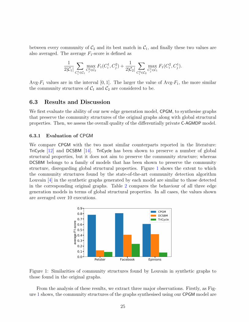
We compare CPGM with the two most similar counterparts reported in the literature:TriCycle [12] and DCSBM [14]. TriCycle has been shown to preserve a number of globalstructural properties, but it does not aim to preserve the community structure; whereasDCSBM belongs to a family of models that has been shown to preserve the communitystructure, disregarding global structural properties. Figure 1 shows the extent to whichthe community structures found by the state-of-the-art community detection algorithmLouvain [4] in the synthetic graphs generated by each model are similar to those detectedin the corresponding original graphs. Table 2 compares the behaviour of all three edgegeneration models in terms of global structural properties. In all cases, the values shownare averaged over 10 executions.

Petster Facebook Epinions0.00.10.20.30.40.50.60.70.80.9

aver

age

F1-s

core

CPGMDCSBMTriCycle

Figure 1: Similarities of community structures found by Louvain in synthetic graphs tothose found in the original graphs.

From the analysis of these results, we extract three major observations. Firstly, as Fig-ure 1 shows, the community structures of the graphs synthesised using our CPGM model are

25

consistently more similar to those of the original graphs, in comparison to those inducedby DCSBM and TriCycle. This supports our claim that CPGM is able to preserve commu-nity structure to a larger extent. Note that, in several cases, our model performs almosttwice as good as the second best, DCSBM. As expected, TriCycle shows the poorest results,corroborating the intuition that community structure needs to be explicitly included inthe generative model if we want synthetic graphs to preserve it. The previous observationssupport our design choices of preserving (i) the community structure, and (ii) differentiatedintra- and inter-community structural properties.

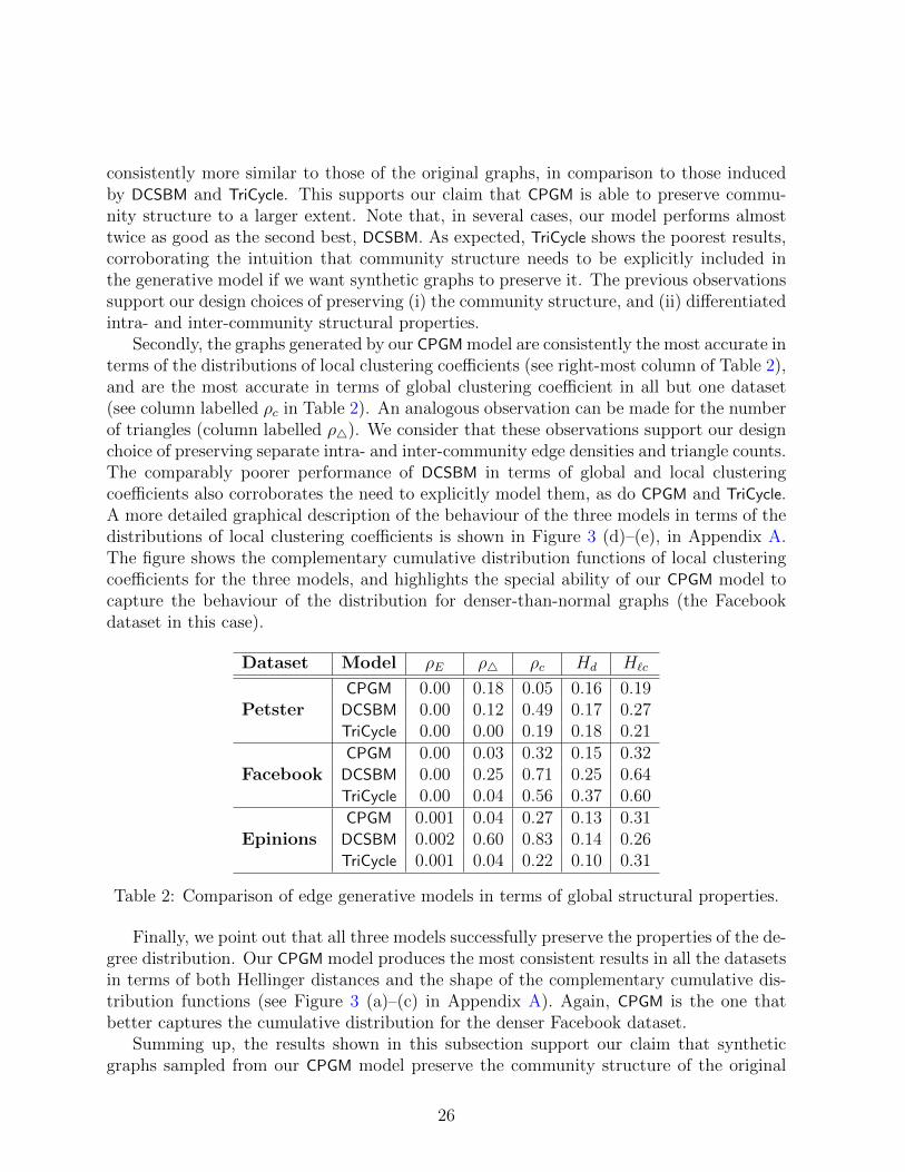
Secondly, the graphs generated by our CPGM model are consistently the most accurate interms of the distributions of local clustering coefficients (see right-most column of Table 2),and are the most accurate in terms of global clustering coefficient in all but one dataset(see column labelled ρc in Table 2). An analogous observation can be made for the numberof triangles (column labelled ρ4). We consider that these observations support our designchoice of preserving separate intra- and inter-community edge densities and triangle counts.The comparably poorer performance of DCSBM in terms of global and local clusteringcoefficients also corroborates the need to explicitly model them, as do CPGM and TriCycle.A more detailed graphical description of the behaviour of the three models in terms of thedistributions of local clustering coefficients is shown in Figure 3 (d)–(e), in Appendix A.The figure shows the complementary cumulative distribution functions of local clusteringcoefficients for the three models, and highlights the special ability of our CPGM model tocapture the behaviour of the distribution for denser-than-normal graphs (the Facebookdataset in this case).

Dataset Model ρE ρ4 ρc Hd H`c

PetsterCPGM 0.00 0.18 0.05 0.16 0.19DCSBM 0.00 0.12 0.49 0.17 0.27TriCycle 0.00 0.00 0.19 0.18 0.21

FacebookCPGM 0.00 0.03 0.32 0.15 0.32DCSBM 0.00 0.25 0.71 0.25 0.64TriCycle 0.00 0.04 0.56 0.37 0.60

EpinionsCPGM 0.001 0.04 0.27 0.13 0.31DCSBM 0.002 0.60 0.83 0.14 0.26TriCycle 0.001 0.04 0.22 0.10 0.31

Table 2: Comparison of edge generative models in terms of global structural properties.

Finally, we point out that all three models successfully preserve the properties of the de-gree distribution. Our CPGM model produces the most consistent results in all the datasetsin terms of both Hellinger distances and the shape of the complementary cumulative dis-tribution functions (see Figure 3 (a)–(c) in Appendix A). Again, CPGM is the one thatbetter captures the cumulative distribution for the denser Facebook dataset.

Summing up, the results shown in this subsection support our claim that syntheticgraphs sampled from our CPGM model preserve the community structure of the original

26


aver

age

F1-s

core

= 2.0 (FB, PR), = 6.0 (EP), Louvain


aver

age

F1-s

core

= 3.0 (FB, PR), = 7.0 (EP), Louvain


aver

age

F1-s

core

= 4.0 (FB, PR), = 8.0 (EP), Louvain


aver

age

F1-s

core

= 5.0 (FB, PR), = 9.0 (EP), Louvain

Petster Facebook Epinions0.0

0.1

0.2

0.3

0.4

0.5

aver

age

F1-s

core

= 2.0 (FB, PR), = 6.0 (EP), CESNA


0.1

0.2

0.3

0.4

0.5

aver

age

F1-s

core

= 3.0 (FB, PR), = 7.0 (EP), CESNA


0.1

0.2

0.3

0.4

0.5

aver

age

F1-s

core

= 4.0 (FB, PR), = 8.0 (EP), CESNA


0.1

0.2

0.3

0.4

0.5

aver

age

F1-s

core

= 5.0 (FB, PR), = 9.0 (EP), CESNA

C-AGMDP C-AGMDP-D AGMDP

Figure 2: Comparison of differentially private models in terms of community structurepreservation.

graph to a considerably larger extent than its closest counterparts, without sacrificing theability to preserve global structural properties. Additionally, these results show that themanner in which CPGM computes intra- and inter-community parameters also helps itoutperform competing models in preserving local and global clustering coefficients.

6.3.2 Evaluation of differentially private C-AGM

We compare C-AGMDP with two other models. The first one is the differentially privateAGM model using TriCycle as edge set generator [12]. We refer to this model as AGMDP-

Tri. It was shown in [12] that, despite the noise added to guarantee privacy, AGMDP-Tri

still preserves to some extent TriCycle’s ability to capture global structural properties. Aswe saw in the previous section, TriCycle performs poorly in preserving the communitystructure of the original graph, so we additionally consider for our evaluation an additionalmodel, which is a modification of C-AGMDP where CPGM is replaced by DCSBM as the edgegeneration model. We refer to this model as C-AGMDP-D.

In our experiments, we compare the behaviour of the three models under four privacybudgets. For the smaller Petster and Facebook datasets, we use the values 2.0, 3.0, 4.0 and5.0. For the considerably larger Epinions dataset, using these values results in considerablynoisy outputs, where pairwise differences between the models have been blurred away bythe noise. Thus, in order to enable comparisons, we show for this dataset the resultsobtained using the values 6.0, 7.0, 8.0 and 9.0. Every particular comparison of the threemodels uses a common privacy budget. Since C-AGMDP-D and AGMDP-Tri each have lessparameters than C-AGMDP, we re-allocate in each case the remaining privacy budget toother computations. In estimating C-AGMDP-D, we allocate to community partition thesame budget as for C-AGMDP, that is ε

2. C-AGMDP-D requires to compute the numbers

of edges between every pair of communities. We assign to this computation the budgetused in C-AGMDP for counting the number of intra-community triangles, i.e. ε

12. Finally,

27

C-AGMDP-D is given for degree sequence computation the budget ε′d = εd + ε4 = ε6, as it

does not require to count the global number of triangles. Since AGMDP-Tri computes everyparameter computed by C-AGMDP, except for the community partition (which takes halfof the budget of C-AGMDP) we double the budget assigned to every other computationof AGMDP-Tri. Notice that these re-allocations give some advantages to C-AGMDP-D andAGMDP-Tri in their comparison with our C-AGMDP model, as they will be able to moreaccurately compute some of the parameters they have in common. We chose to allowthis advantage considering that requiring a smaller number of computations is in fact apositive feature of a differentially private method, which should not be punished in thecomparison. In C-AGMDP and C-AGMDP-D, ModDivisive is run with ws = 0.98. Finally, inestimating the distribution of attribute-edge correlations (as discussed in Section 5.3), weset the maximum degree parameter p to 100.

Figure 2 displays the behaviours of the three models in terms of community structurepreservation, whereas Tables 3, 4 and 5 summarise their behaviours in terms of globalstructural properties and attribute-edge correlations on Petster, Facebook and Epinions,respectively. In what follows, we analyse these results from three different perspectives.

ε Model ρE ρ4 ρc Hd H`c ρa

2.0C-AGMDP 0.56 0.09 0.43 0.42 0.39 0.14C-AGMDP-D 0.22 0.55 0.69 0.30 0.44 0.23AGMDP-Tri 0.25 0.09 0.25 0.23 0.30 0.17




Table 3: Comparison of differentially private models on Petster.

Community structure preservation. In Figure 2, the four uppermost charts displaythe extent to which the community structures found by Louvain in the synthetic graphsgenerated by each differentially private model are similar to those detected in the corre-sponding original graphs. Two important features of the Louvain algorithm are sharedby ModDivisive, the method used for obtaining community partitions in C-AGMDP andC-AGMDP-D. Both generate a community partition, and both operate by maximising mod-ularity. In order to assess whether the community structures induced by our models inthe synthetic graphs are also detectable by algorithms based on different criteria, we ad-ditionally obtained analogous results using the algorithm CESNA [42]. These results areshown in the lowermost four charts of Figure 2. Unlike Louvain, CESNA takes node at-

28

tributes into consideration for computing communities. However, CESNA tends to obtainsubstantially overlapping communities, whereas both C-AGMDP and C-AGMDP-D assume apartition. CESNA requires as a parameter the number of communities, which we set to 10.

ε model ρE ρ4 ρc Hd H`c ρa





Table 4: Comparison of differentially private models on Facebook.

From the analysis of these results, the most relevant observation is that, consideringthe communities detected by both Louvain and CESNA, the graphs sampled from ourC-AGMDP model consistently rank as the ones whose community structure is most similarto that of the corresponding original graphs. In the particular cases of Petster and Facebookwith the Louvain algorithm, the similarity values displayed by our C-AGMDP model are insome cases close to twice better than their counterparts for C-AGMDP-D, and considerablymore than those for AGMDP-Tri. An additional important observation is that our modelshows less variation for different amounts of noise, when compared to C-AGMDP-D andAGMDP-Tri.

Distributions of attribute-edge correlations. On each original graph, we computethe distributions of attribute-edge correlations in each community detected by CESNA.Then, we compute the equivalent distributions on each synthetic graph and compare it tothat of the original graph in terms of ρa (see right-most columns of Tables 3, 4 and 5).

From the analysis of these results, we can see that the synthetic graphs sampled from C-

AGMDP and C-AGMDP-D, the two models that consider community structures, consistentlyoutperform those sampled from AGMDP-Tri in terms of ρa. Another important observationis that the qualities, in terms of ρa, of synthetic graphs sampled from our C-AGMDP modeland those sampled from its variant C-AGMDP-D are quite similar. This observation suggeststhat C-AGMDP can in some cases be seen as a meta-model, where several edge generationmodels can be used, e.g. CPGM and DCSBM in this experiment.

Global structural properties. From the analysis of Tables 3, 4 and 5, we can see that, asexpected, our C-AGMDP model suffers a larger degradation than C-AGMDP-D and AGMDP-

Tri in terms of the measures that depend on parameters for which the latter models were

29

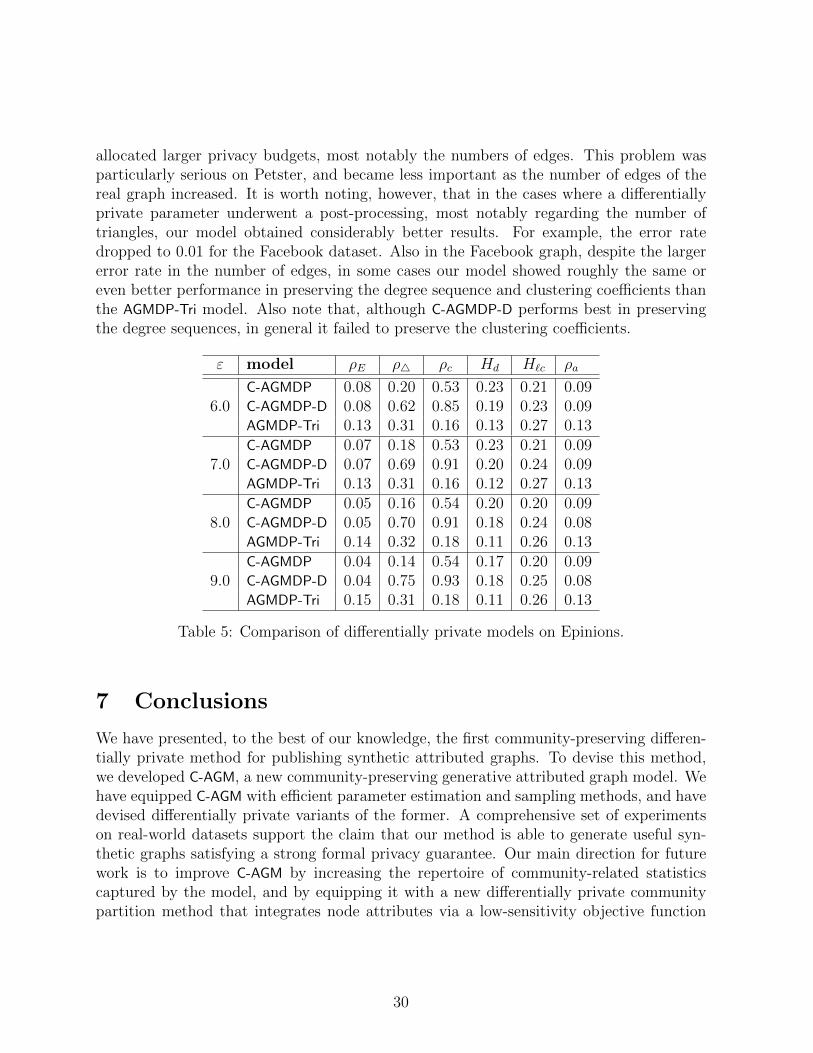
allocated larger privacy budgets, most notably the numbers of edges. This problem wasparticularly serious on Petster, and became less important as the number of edges of thereal graph increased. It is worth noting, however, that in the cases where a differentiallyprivate parameter underwent a post-processing, most notably regarding the number oftriangles, our model obtained considerably better results. For example, the error ratedropped to 0.01 for the Facebook dataset. Also in the Facebook graph, despite the largererror rate in the number of edges, in some cases our model showed roughly the same oreven better performance in preserving the degree sequence and clustering coefficients thanthe AGMDP-Tri model. Also note that, although C-AGMDP-D performs best in preservingthe degree sequences, in general it failed to preserve the clustering coefficients.

ε model ρE ρ4 ρc Hd H`c ρa





Table 5: Comparison of differentially private models on Epinions.

7 Conclusions

We have presented, to the best of our knowledge, the first community-preserving differen-tially private method for publishing synthetic attributed graphs. To devise this method,we developed C-AGM, a new community-preserving generative attributed graph model. Wehave equipped C-AGM with efficient parameter estimation and sampling methods, and havedevised differentially private variants of the former. A comprehensive set of experimentson real-world datasets support the claim that our method is able to generate useful syn-thetic graphs satisfying a strong formal privacy guarantee. Our main direction for futurework is to improve C-AGM by increasing the repertoire of community-related statisticscaptured by the model, and by equipping it with a new differentially private communitypartition method that integrates node attributes via a low-sensitivity objective function

30

and/or differentially private maximum-likelihood estimation methods.

Acknowledgements: The work reported in this paper received funding from Luxem-bourg’s Fonds National de la Recherche (FNR), via grant C17/IS/11685812 (PrivDA).

References

[1] Regulation (eu) 2016/679 of the european parliament and of the council of 27 april2016 on the protection of natural persons with regard to the processing of personaldata and on the free movement of such data, and repealing directive 95/46/ec (generaldata protection regulation). OJ, L 119:1–88, 4.5.2016.

[2] Lars Backstrom, Cynthia Dwork, and Jon M. Kleinberg. Wherefore art thou r3579x?:anonymized social networks, hidden patterns, and structural steganography. Commu-nications of the ACM, 54(12):133–141, 2011.

[3] Jeremiah Blocki, Avrim Blum, Anupam Datta, and Or Sheffet. Differentially privatedata analysis of social networks via restricted sensitivity. In Proc. 4th Innovations inTheoretical Computer Science (ITCS), pages 87–96. ACM Press, 2013.

[4] Vincent D Blondel, Jean-Loup Guillaume, Renaud Lambiotte, and Etienne Lefebvre.Fast unfolding of communities in large networks. Journal of Statistical Mechanics:Theory and Experiment, 2008(10):P10008, 2008.

[5] Lauren E. Charles-Smith, Tera L. Reynolds, Mark A. Cameron, Mike Conway, EricH. Y. Lau, Jennifer M. Olsen, Julie A. Pavlin, Mika Shigematsu, Laura C. Streichert,Katie J. Suda, and Courtney D. Corley. Using social media for actionable diseasesurveillance and outbreak management: A systematic literature review. PLOS ONE,10(10):1–20, 10 2015.

[6] Fan Chung and Linyuan Lu. The average distances in random graphs with givenexpected degrees. Proceedings of the National Academy of Sciences, 99(25):15879–15882, 2002.

[7] Aaron Clauset, Cristopher Moore, and M. E. J. Newman. Hierarchical structure andthe prediction of missing links in networks. Nature, 453:98–101, 2008.

[8] Cynthia Dwork. Differential privacy. In Proc. 33rd International Colloquium on Au-tomata, Languages and Programming (ICALP), volume 4052 of Lecture Notes in Com-puter Science, pages 1–12. Springer, 2006.

[9] Michael Hay, Chao Li, Gerome Miklau, and David D. Jensen. Accurate estimationof the degree distribution of private networks. In Proc. 19th IEEE InternationalConference on Data Mining (ICDM), pages 169–178. IEEE Computer Society, 2009.

31

[10] Joseph J. Pfeiffer III, Timothy La Fond, Sebastian Moreno, and Jennifer Neville. Fastgeneration of large scale social networks while incorporating transitive closures. InProc. 4th International Conference on Privacy, Security, Risk and Trust, (PASSAT),pages 154–165. IEEE Computer Society, 2012.

[11] Joseph J. Pfeiffer III, Sebastian Moreno, Timothy La Fond, Jennifer Neville, and BrianGallagher. Attributed graph models: modeling network structure with correlatedattributes. In Proc. 23rd International World Wide Web Conference (WWW), pages831–842. ACM Press, 2014.

[12] Zach Jorgensen, Ting Yu, and Graham Cormode. Publishing attributed social graphswith formal privacy guarantees. In Proc. 2016 International Conference on Manage-ment of Data (SIGMOD), pages 107–122. ACM Press, 2016.

[13] Kundan Kandhway and Joy Kuri. Using node centrality and optimal control to max-imize information diffusion in social networks. IEEE Trans. Systems, Man, and Cy-bernetics: Systems, 47(7):1099–1110, 2017.

[14] Brian Karrer and Mark EJNewman. Stochastic blockmodels and community structurein networks. Physical review. E, 83(1):016107, 2011.

[15] Vishesh Karwa, Sofya Raskhodnikova, Adam D. Smith, and Grigory Yaroslavtsev. Pri-vate analysis of graph structure. ACM Transactions on Database Systems, 39(3):22:1–22:33, 2014.

[16] Vishesh Karwa and Aleksandra B. Slavkovic. Differentially private graphical degreesequences and synthetic graphs. In Proc. 2012 International Conference on Privacyin Statistical Databases (PSD), volume 7556 of Lecture Notes in Computer Science,pages 273–285. Springer, 2012.

[17] Daniel Kifer and Bing-Rong Lin. Towards an axiomatization of statistical privacy andutility. In Proc. 29th ACM SIGMOD-SIGACT-SIGART Symposium on Principles ofDatabase Systems (PODS), pages 147–158. ACM Press, 2010.

[18] Tamara G. Kolda, Ali Pinar, Todd D. Plantenga, and C. Seshadhri. A scalable gener-ative graph model with community structure. SIAM J. Scientific Computing, 36(5),2014.

[19] Jerome Kunegis. KONECT: the koblenz network collection. In Proc. 22nd Interna-tional World Wide Web Conference (WWW), pages 1343–1350. ACM Press, 2013.

[20] Jure Leskovec and Christos Faloutsos. Scalable modeling of real graphs using kroneckermultiplication. In Proc. 24th International Conference on Machine Learning (ICML),pages 497–504. ACM Press, 2007.

[21] Jure Leskovec and Andrej Krevl. SNAP Datasets: Stanford large network datasetcollection. http://snap.stanford.edu/data, 2014.

32

http://snap.stanford.edu/data

[22] Nelly Marquetoux, Mark A. Stevenson, Peter Wilson, Anne Ridler, and Cord Heuer.Using social network analysis to inform disease control interventions. Preventive Vet-erinary Medicine, 126:94–104, 2016.

[23] Paolo Massa and Paolo Avesani. Trust-aware recommender systems. In Proc. 2007ACM Conference on Recommender Systems (RecSys), pages 17–24. ACM Press, 2007.

[24] Sjouke Mauw, Yunior Ramırez-Cruz, and Rolando Trujillo-Rasua. Robust active at-tacks on social graphs. Data Mining and Knowledge Discovery, 33(5):1357–1392, 2019.

[25] Frank McSherry. Privacy integrated queries: an extensible platform for privacy-preserving data analysis. Communications of the ACM, 53(9):89–97, 2010.

[26] Frank McSherry and Kunal Talwar. Mechanism design via differential privacy. InProc. 48th Annual IEEE Symposium on Foundations of Computer Science (FOCS),pages 94–103. IEEE Computer Society, 2007.

[27] Darakhshan J. Mir and Rebecca N. Wright. A differentially private graph estimator.In Proc. 2009 ICDM International Workshop on Privacy Aspects of Data Mining(ICDM), pages 122–129. IEEE Computer Society, 2009.

[28] Prateek Mittal, Charalampos Papamanthou, and Dawn Xiaodong Song. Preservinglink privacy in social network based systems. In Proc. 20th Annual Network andDistributed System Security Symposium (NDSS). The Internet Society, 2013.

[29] Arvind Narayanan and Vitaly Shmatikov. De-anonymizing social networks. In Proc.30th IEEE Symposium on Security and Privacy (S&P), pages 173–187. IEEE Com-puter Society, 2009.

[30] M. E. J. Newman and M. Girvan. Finding and evaluating community structure innetworks. Physical Reviewe E, 69(2):026113, 2004.

[31] Mark E. J. Newman. Community detection in networks: Modularity optimization andmaximum likelihood are equivalent. CoRR, abs/1606.02319, 2016.

[32] Hiep H. Nguyen, Abdessamad Imine, and Michael Rusinowitch. Detecting communi-ties under differential privacy. In Proc. 2016 ACM on Workshop on Privacy in theElectronic Society (WPES), pages 83–93. ACM Press, 2016.

[33] Kobbi Nissim, Sofya Raskhodnikova, and Adam Smith. Smooth sensitivity and sam-pling in private data analysis. In Proc. 39th Annual ACM Symposium on Theory ofComputing (STOC), pages 75–84. ACM Press, 2007.

[34] Liudmila Ostroumova Prokhorenkova and Alexey Tikhonov. Community detectionthrough likelihood optimization: In search of a sound model. In Proc. 30th WorldWide Web Conference (WWW), pages 1498–1508. ACM Press, 2019.

33

[35] Alessandra Sala, Xiaohan Zhao, Christo Wilson, Haitao Zheng, and Ben Y. Zhao.Sharing graphs using differentially private graph models. In Proc. 11th ACM SIG-COMM Internet Measurement Conference (IMC), pages 81–98. ACM Press, 2011.

[36] Yue Wang and Xintao Wu. Preserving differential privacy in degree-correlation basedgraph generation. Transaction on Data Privacy, 6(2):127–145, 2013.

[37] Yue Wang, Xintao Wu, Jun Zhu, and Yang Xiang. On learning cluster coefficient ofprivate networks. Social Network Analysis and Mining, 3(4):925–938, 2013.

[38] Paul W.Holland, Kathryn Blackmond Laskey, and Samuel Leinhardt. Stochasticblockmodels: First steps. Social Networks, 5(2):109–137, 1983.

[39] Qian Xiao, Rui Chen, and Kian-Lee Tan. Differentially private network data releasevia structural inference. In Proc. 20th ACM SIGKDD International Conference onKnowledge Discovery and Data Mining (KDD), pages 911–920. ACM Press, 2014.

[40] Jaewon Yang and Jure Leskovec. Overlapping community detection at scale: a non-negative matrix factorization approach. In Proc. 6th ACM International Conferenceon Web Search and Data Mining (WSDM), pages 587–596. ACM Press, 2013.

[41] Jaewon Yang and Jure Leskovec. Defining and evaluating network communities basedon ground-truth. Knowledge and Information Systems, 42(1):181–213, 2015.

[42] Jaewon Yang, Julian J. McAuley, and Jure Leskovec. Community detection in net-works with node attributes. In Proc. 13th IEEE International Conference on DataMining (ICDM), pages 1151–1156. IEEE Computer Society, 2013.

[43] Jun Zhang, Graham Cormode, Cecilia M. Procopiuc, Divesh Srivastava, and XiaokuiXiao. Private release of graph statistics using ladder functions. In Proc. 36th ACMInternational Conference on Management of Data (SIGMOD), pages 731–745. ACMPress, 2015.

[44] Dmitry Zinoviev. Information Diffusion in Social Networks, pages 146–163. 11 2011.

A Distribution of degree and local clustering coeffi-

cient

Figure 3 shows the comparison of degree distributions (a–c) and distributions of localclustering coefficients (d–f) in terms of the complementary cumulative distribution functions(CCDF). Every degree or LCC value (x-axis) is mapped to the percentage of vertices havinga larger value (y-axis).

34

0 25 50 75 100 125 150 175 200Degree

0.0

0.2

0.4

0.6

0.8

CC

DF

OriginalCPGMDCSBMTriCycle

(a) Petster

0 100 200 300 400 500Degree

0.0

0.2

0.4

0.6

0.8

1.0

CC

DF


(b) Facebook

0 20 40 60 80 100 120 140Degree

0.00.10.20.30.40.50.60.70.8

CC

DF


(c) Epinions

0.0 0.2 0.4 0.6 0.8 1.0Local Clustering Coeff.

0.00.10.20.30.40.50.60.7

CC

DF


(d) Petster


0.0

0.2

0.4

0.6

0.8

1.0

CC

DF


(e) Facebook


0.0

0.1

0.2

0.3

0.4

CC

DF


(f) Epinions

Figure 3: Detailed comparison of edge generative models in terms of complementary cu-mulative distribution functions of degree and local clustering coefficient distributions.

35

Publishing Community-Preserving Attributed Social Graphs ...

Documents

Transcript of Publishing Community-Preserving Attributed Social Graphs ...