Published in - Glasgow Caledonian...

ResearchOnline@GCU

Glasgow Caledonian University

Green infrastructure as an adaptation approach to tackle urban overheating in theGlasgow Clyde Valley Region|Emmanuel, R; Loconsole, Alessandro

Published in:Landscape and Urban Planning

DOI:10.1016/j.landurbplan.2015.02.012

Publication date:2015

Document VersionPeer reviewed version

Link to publication in ResearchOnline@GCU

Citation for published version (APA):Emmanuel, R., & Loconsole, A. (2015). Green infrastructure as an adaptation approach to tackle urbanoverheating in the Glasgow Clyde Valley Region. Landscape and Urban Planning, 138, 71-86.10.1016/j.landurbplan.2015.02.012

General rightsCopyright and moral rights for the publications made accessible in the public portal are retained by the authors and/or other copyright ownersand it is a condition of accessing publications that users recognise and abide by the legal requirements associated with these rights.

• Users may download and print one copy of any publication from the public portal for the purpose of private study or research. • You may not further distribute the material or use it for any profit-making activity or commercial gain • You may freely distribute the URL identifying the publication in the ResearchOnline@GCU portal

Take down policyIf you believe that this document breaches copyright please contact us at: [email protected] providing details, and we will removeaccess to the work immediately and investigate your claim.

Download date: 15. Jul. 2018

http://dx.doi.org/10.1016/j.landurbplan.2015.02.012

http://researchonline.gcu.ac.uk/en/publications/green-infrastructure-as-an-adaptation-approach-to-tackle-urban-overheating-in-the-glasgow-clyde-valley-region(f056e35e-ea97-4372-adcb-a15d7cc68e58).html

Green infrastructure as an adaptation approach to tackling urbanoverheating

in the Glasgow Clyde Valley Region, UK

R. Emmanuela*, A. Loconsoleb

aSchool of Engineering & Built Environment, Glasgow Caledonian University, UK

bDepartment of Material Sciences, University of Salento, Italy

Citation:

Emmanuel, R., & Loconsole, A. Green infrastructure as an adaptation approach to tackling urban overheating in the Glasgow Clyde Valley Region, UK. Landscape Urban Plan. (2015), http://dx.doi.org/10.1016/j.landurbplan.2015.02.012

Highlights:

Classification of urban areas into local climate zones (LCZ) 1

CFD simulation of green cover in mitigating climate change and heat island effects 2

20% increase in green cover could reduce surface temperatures by 2oC in 2050 3

Green infrastructure option to achieve 20% increase in greenery are presented 4

5

Abstract

Although urban growth in the city of Glasgow, UK, has subsided, urban morphology continues to 6 generate local heat islands. We present a relatively less data‐intense method to classify local climate 7 zones (LCZ) and evaluate the effectiveness of green infrastructure options in tackling the likely 8 overheating problem in cold climate urban agglomerations such as the Glasgow Clyde Valley (GCV) 9 region. LCZ classification uses LIDAR data available with local authorities, based on the typology 10 developed by Stewart and Oke (2012). LCZ classes were then used cluster areas likely to exhibit 11 similar warming trends locally. This helped to identify likely problem areas, a sub‐set of which were 12 then modelled for the effect of green cover options (both increase and reduction in green cover) as 13 well as building density options. 14

Results indicate green infrastructure could play a significant role in mitigating the urban overheating 15 expected under a warming climate in the GCV Region. A green cover increase of approximately 20% 16 over the present level could eliminate a third to a half of the expected extra urban heat island effect 17 in 2050. This level of increase in green cover could also lead to local reductions in surface 18 temperature by up to 2oC. Over half of the street users would consider a 20% increase in green 19 cover in the city centre to be thermally acceptable, even under a warm 2050 scenario. The process 20 adopted here could be used to estimate the overheating problem as well as the effectiveness green 21 infrastructure strategies to overcome them. 22

23

1. Introduction

In the face of growing consensus on the anthropogenic causes for global climate change (see IPCC, 24

2013) and the lag‐times involved in the mitigation of such changes, there is considerable focus on 25

the enhancement of adaptive capacity of human systems to cope with climate change. Given the 26

rapid rise in global urbanisation much of the adaptive action needs to occur in cities. However, 27

research on the augmentation of climate change effects by local urban warming (characterised by 28

urban heat islands) remains weak. A key difficulty in untangling the urban warming from global 29

climate change is the computational and parametric difficulties associated with representing urban 30

areas in climate models (Jin et al., 2005; Grawe et al., 2013). Additionally, translating future climate 31

change projections at finer spatial scales relevant to cities typically use statistical downscaling 32

techniques to global climate models without modelling the urban areas themselves (Lemonsu et al., 33

2013) a technique not without problems. Although the situation is continuing to improve (cf. 34

Hebbert and Jankovic, 2013) much more still need to be done to (a) ameliorate the urban heat island 35

(UHI) effect and (b) use UHI mitigation as part of climate change adaptation. 36

World’s shrinking cities face additional problems in managing climate change. Previous work in 37

Glasgow (Emmanuel and Kruger, 2012; Kruger et al., 2013) – one such ‘shrinking city’ – indicates that 38

even when urban growth has subsided, the local warming that result from urban morphology 39

(increased built cover, lack of vegetation, pollution, anthropogenic heat generation) continue to 40

generate local heat islands. Such heat islands are of the same order of magnitude as the predicted 41

warming due to climate change by 2050. And the micro‐scale variations are strongly related to local 42

land cover/land use patterns. However, current climate change adaptation strategies are more 43

focussed on reducing carbon emission than managing the change via land use / land cover 44

manipulations, even though the latter is relatively easier to manage in shrinking cities. 45

Given these realities, it is necessary to explore the role of land cover changes especially green 46

infrastructure changes, as potential climate change adaptation options. Specifically, it is necessary 47

to quantify the scale of green infrastructure changes needed in specific cities and explore ways to 48

accomplish them. It in this light the present paper explores the role of green cover in areas of 49

different urban density within the Glasgow Clyde Valley (GCV) Region in the central belt of Scotland. 50

It characterises the urban pattern within the GCV in terms of their local warming attributes, using a 51

classification system known as the Local Climate Zones (LCZ) (Stewart and Oke, 2012). Such 52

classification could help identify areas most likely to experience significant overheating problem in 53

the future (cf. Lelovics et al., 2014). Computational fluid dynamics (CFD) simulations are then carried 54

out to test the applicability of green infrastructure approaches. Alternative strategies to enhance 55

the green cover in a Glasgow city centre neighbourhood are presented. 56

The rest of the paper is structured in five sections: Section 2 presents background evidence to the 57

presence of the heat island phenomenon in Glasgow and the two techniques commonly used to 58

study it (local climate zones to classify urban areas and ENVI‐met, a CFD model commonly used to 59

study the effectiveness of mitigation strategies). Sections 3 and 4 detail the land cover/land use 60

classification employed in the present study. Section 5 presents the results of the simulation 61

exercise and Section 6 explores the implications of the results. It is hoped that the method of 62

classifying LCZ using relatively easily available data as well as the exploration of green infrastructure 63

in ameliorating the likely overheating problem could be applicable to other cold climate cities. 64

2. Background

2.1 Glasgow’s heat island phenomenon

Based on a four‐pronged approach to map the local climate variations in and around the city of 65

Glasgow in 2011 (historic climate trends in the city; fixed weather station data in and around the 66

city; microclimate variations at the street canyon level within the city core, and thermal perception 67

of street users in the heart of the city centre) Emmanuel and Kruger (2012) and Kruger et al., (2013) 68

found the following: 69

1. Even when urban growth has subsided, the local warming that result from urban 70 morphology (increased built cover, lack of vegetation, pollution, anthropogenic heat 71 generation) continue to generate local heat islands; 72

2. Such heat islands are of the same order of magnitude as the predicted warming due to 73 climate change to 2050; 74

3. Substantial variations within city neighbourhoods exist and these relate to land use/land 75 cover attributes, pointing to planning possibilities to locally mitigate the negative 76 consequences of overheating; 77

4. Strategies to tackle local overheating can lead to less carbon intensive enhancement of 78 comfort, health and quality of life both within and outside buildings. 79

Given the geographic and urban growth similarities of the GCV region to that of the city of Glasgow, 80

the overheating problem in the GCV area is likely to be similar. Carefully planned development of 81

urban morphological variables such as the green infrastructure offers possibilities to enhance 82

outdoor livability and reduced building energy use in the immediate future when the regional 83

climate remains relatively similar to current conditions, but also provides an adaptive mechanism 84

when the background climate continues to warm (Kleerekoper et al., 2012), thus lending itself to be 85

a useful strategy to adapt to climate change in the GCV region, both in the immediate‐ and long‐86

term. 87

2.2 Local Climate Zone classification

In order to characterise the land use / land cover patterns in areas of interest, we used the ‘Local 88

Climate Zone’ (LCZ) system developed by Stewart and Oke (2012). LCZs are defined as ‘regions of 89

uniform surface‐air temperature distribution at horizontal scales of 102 to 104 metres’ (Stewart and 90

Oke, 2012). Their definition is based on characteristic geometry and land cover that is expected to 91

generate a unique near‐surface climate under calm, clear skies. These include vegetative fraction, 92

building/tree height and spacing, soil moisture, and anthropogenic heat flux. LCZ has 16 climate 93

zones and the classification system has been validated in Sweden, Japan and Canada (Stewart and 94

Oke, 2009) and widely used in other contexts (for example, Lelovics et al., 2014; Middel, et al., 2014; 95

Villadiego and Velay‐Dabat, 2014). 96

Although the LCZ classification system was not developed for mapping the UHI effect but to assist in 97

the selection of locations for local weather stations and to report heat island effect in a standardised 98

manner, it is a useful system to identify micro‐climatically distinguishable areas within an urban 99

agglomeration, and this aspect of the LCZ is useful in identifying the likely local warming effects of 100

urban development. This was indeed shown to be true in Glasgow (see Figure 12 in Emmanuel and 101

Kruger, 2012). 102

2.3 CFD simulations in UHI studies

The non‐linearity of the UHI problem lends itself to numerical simulations and is therefore 103

increasingly popular in urban climatology (Saneinejad et al, 2014). Urban microclimate models vary 104

widely with regard to their physical basis and spatial/temporal resolution. Ali‐Toudert & Mayer 105

(2006) provide a detailed critique of contemporary models at the micro‐scale with fine temporal 106

resolutions. They inferred that ENVI‐met (Bruse 1999, 2004) is perhaps the only micro‐scale 107

computational fluid dynamic model that is capable of analyzing the thermal comfort regime within 108

the street canyon at fine resolutions (down to 0.5 0.5 m). ENVI‐met is increasingly being used to 109

assess the effectiveness of urban planning measures to tackle the UHI problem in a variety of climate 110

contexts (for example, Ketterer and Matzarakis, 2014 – Stuttgart, Germany; Chen and Ng, 2013 – 111

Hongkong SAR; Emmanuel et al., 2010 – Colombo, Sri Lanka; Middell et al., 2014 – Phoenix, USA; 112

Skelhorn et al., 2014, Manchester, UK). 113

ENVI‐met is a three‐dimensional non‐hydrostatic model for the simulation of surface–plant–air 114

interactions, especially within the urban canopy layer. It is designed for the micro‐scale with a 115

typical horizontal resolution from 0.5 to 10 m and a typical time frame of 24 to 48 h with a time step 116

of 10 s. This resolution allows the investigation of small‐scale interactions between individual 117

buildings, surfaces and plants (Bruse 2004). 118

Input meteorological data required to initiate ENVI‐met simulations are: wind speed and direction at 119

10 m above ground, roughness length (Zo), initial temperature of the atmosphere, specific humidity 120

at 2500 m and relative humidity at 2 m. The model calculation includes surface and wall 121

temperatures for each grid point and wall and the calculation of bio‐meteorological parameters such 122

as the Mean Radiant Temperature (MRT) or Predicted Mean Vote (PMV) (Fanger 1970). 123

A shortcoming of ENVI‐met is that buildings, which are modelled as blocks where width and length 124

are multiples of grid cells, have no thermal mass and have constant indoor temperature. Moreover, 125

albedo and thermal transmission (U‐value) for walls and roofs are the same for all buildings. 126

However, it is an effective tool for the analysis of urban temperature at the micro‐scale with fine 127

temporal resolutions (Ali‐Toudert & Mayer, 2006). 128

3. Method

The pursuit of green infrastructure strategies to tackle the overheating problem due to climate 129

change enhanced by local warming in the GCV required the following steps: 130

1. Identification of localities where local warming is likely to be the most intense (the ‘hot 131 spots’); 132

2. Estimation of the likely future climate (in 2050); 133

3. Evaluation of the sensitivity of green infrastructure‐based adaptation options to reduce 134 the ‘hot spots’ under future climate. 135

136

We classified the GCV region into LCZ classes using Ordnance Survey (OS) and LiDAR data to estimate 137

surface characteristics such as building cover, building height, land cover and/or land use. Ordnance 138

Survey is the UK’s national mapping authority providing detailed land cover information and its data 139

are available free of charge at: https://www.ordnancesurvey.co.uk. Vector files containing the 140

following layers were downloaded for the National Grid No. NS26, which covers all of the GCV 141

Region. More details on the National Grid are available at: 142

http://www.ordnancesurvey.co.uk/docs/support/national‐grid‐map‐references.pdf. Each square 143

contains land cover data for a 100 x 100 km area. Light Detection And Ranging (LiDAR) data is an 144

accurate, high resolution three‐dimensional data used to create highly detailed digital surface 145

models that could eventually be turned into three dimensional city models. LiDAR technology allows 146

large area models to be created in a very short space of time. LiDAR data for the present study area 147

was provided by the Glasgow Clyde Valley Green Network Partnership 148

(http://www.gcvgreennetwork.gov.uk/) which itself obtained the data from the local authorities in 149

the GCV region. Additional ground truth verification of selected representative areas using ‘Google 150

Earth’ and site visits helped verify building height and other physical parameters. Future climate 151

data were obtained from the UK Climate Projections 2009 – UKCIP’09 (http://www.ukcip.org.uk/). 152

UKCIP’09 is the fifth generation of climate change information for the UK and is based on inductive 153

probability (i.e. estimations are based on the available information and strength of evidence instead 154

of taking into account all the possible outcomes) 155

The evaluation of the effect of green infrastructure was carried out using ENVI‐met simulations. Six 156

scenarios were run as detailed below. : 157

1. 2012 climate with current development pattern = ‘Current Case;’ 158

2. 2050 climate (using UKCIP’09 projections) with current level of development – ‘Base 159 Case’; 160

3. 2050 climate with ‘loss’ of green infrastructure (‘m10 case’) 161

4‐6. 2050 climate with three levels of increased green cover (+10%, +20% and +100% relative 162 to the existing case – p10, p20 and p100 cases, respectively) 163

Based on the simulation results we estimated the minimum green cover needed to make a 164

significant difference to the likely local warming in 2050. We then used the Green Area Ratio 165

method (Keeley, 2011) to normalise the climatic effects of different types of green cover (urban 166

parks, street trees, green roofs, green walls, etc). 167

3.1 Green Area Ratio (GAR) method

Not all green areas contribute equally to local cooling nor are they equal in their other 168

environmental and sustainability benefits. Recognising this, planning authorities have developed 169

weighting systems that captures the relative environmental performance of different types of green 170

cover. The most widely used among these is the Green Area Ratio (GAR) method (Keeley, 2011). 171

GAR assigns weighting factors for different types of urban green infrastructure, based on their 172

relative environmental performance in terms of climate change mitigation. It is currently 173

implemented in Berlin and has been adapted in Malmo (Sweden), several cities in South Korea and 174

Seattle (USA) (Keeley, 2011). Table 1 shows the relative weighting of different types of green cover. 175

(Table 1 here) 176

4. Effect of land use / land cover and local climate

The key to understanding the local climatic effect of land cover/land use characteristics is to classify 177

the settlement area according to their key climate‐influencing features. 178

4.1 Site selection using the LCZ approach

The following steps were performed to determine the dominant LCZ classes in the GCV region and 179

thus select ‘representative’ sample locations where local warming is likely to be problematic. 180

1. Determine the ‘developed’ areas of the GCV 181

2. Calculate built fraction / natural cover within 1km dia circles placed in an array covering 182 the entire ‘developed’ area in the GCV identified in step 1 183

3. Classify each circle into relevant LCZ class, depending on built/green fraction and building 184 height closely matching the urban morphological parameters shown in Table 2 185

4. Select sample locations representing the different LCZ classes available within the GCZ 186

(Table 2 here) 187

The aim of the first step was to reduce the area of enquiry to ‘developed’ areas within the urban 188

agglomeration to limit the computational time needed. We first downloaded the data for the area 189

of interest from the ordnance survey open database. The GCV Region covers only a small part of the 190

100x100km NS square (NS26, see Section 3), and the ‘developed’ area within the relevant NS square 191

was clipped and a 1km x 1km grid was placed over it. This resulted in 1519 grid points on the 1km x 192

1km grid and a circle of 500m in radius was added to each point to carry out Step 2. Step 2 then 193

calculated the built cover (building footprints and roads) as well as the ‘natural’ cover. The building 194

cover were divided into categories (depending on their three dimensional properties. 195

Step 3 (determination of the LCZ class of each 1km dia. Circle) was carried out as follows: Four small 196

circles (500m dia.) were created within each large circle (See Figure 1). The percentages of buildings, 197

roads, inland water and natural cover were calculated for each of the 500m dia. circles using ArcGIS 198

(v.10.1) and averaged to derive at the land cover types for each of the 1km radius circle. Figure 2 199

shows the results of Step 3. 200

(Figure 1 here) 201

(Figure 2 here) 202

It could be seen from Figure 2 that the GCV region largely composes of two classes of ‘semi‐dense’ 203

urban morphology (LCZ 2 and 3 – Compact midrise, mainly Glasgow City centre) and three classes of 204

‘sparse’ settlement morphology (LCZ 5 – Open midrise; LCZ 6 – Open lowrise; LCZ 9 – Sparsely built). 205

Based on these results Step 4 selected six sites. In addition to representing the variations in LCZ 206

classes this step also considered the location of local weather stations, the data from which could be 207

useful in initiating the ENVI‐met model runs for each of the selected sites. The selected sites are 208

listed below (See Figure 3 for locations and Figure 4 for three‐dimensional details): 209

1‐2. LCZ 2 – Compact midrise two locations characterising this class: Glasgow City Centre 210 West (Gla CCW) centred on the intersection of W Campbell Street & Bath Street 211 (Coordinates – British National Grid; map projection: transverse Mercator; datum: OSGB: 212 36258595.665 – 665800.603 Meters) and Glasgow City Centre East (Gla CCE) comprising 213 an area surrounding the George Square area, centred on the intersection of John Street 214 & Ingram Street (259339.524 – 665260.852 Meters); 215

3. LCZ 6 – Open lowrise: Clyde Gateway area (London Road & Springfield Road) (260683.157 216 – 663742.061 Meters); 217

4. LCZ 5 – Open midrise: Paisley area (High Street & New Street) (248146.997 – 663988.741 218 Meters) 219

5‐6. LCZ 9 – Sparsely built (or extensive lowrise): two locations characterising this class 220 Wishaw (Caledonia Rd. and Main St.) (279691.562 – 655018.654 Meters), and Hamilton 221 (Brandon St. and Quarry St.) (272438.576 – 655517.511 Meters) 222

223

(Figure 3 here) 224

(Figure 4 here) 225

Land cover characteristics of the individual sites are shown in Figures 5‐9 (Note Sites 1 and 2 are 226

covered by Figure 5). Each figure shows the land cover as given in the Ordnance Survey maps (see 227

‘Legend’ at bottom left). These were amalgamated into categories relevant to LCZ (bottom right) as 228

follows: 229

Built cover = Building, Structure, Structure on path, Glasshouse; 230

Natural = Natural Environment, Natural Environment along road or track; 231

Transportation = Road or Track, Roadside, Rail, Path 232

Water = Tidal Water, Inland Water 233

Open Surface = General Surface 234

Unclassified = Landform, Unclassified, Landform along road/track 235

(Figure 5 here) 236

(Figure 6 here) 237

(Figure 7 here) 238

(Figure 8 here) 239

(Figure 9 here) 240

5. Simulation of the effects of green infrastructure in the GCV

The performance of ENVI‐met was validated for Glasgow, using a process described by Loconsole 241

(2013). We used data from a weather station set up on the city campus of Glasgow Caledonian 242

University (55.86611oN, 4.25oW) for this purpose. For the turbulence closure of the atmospheric 243

boundary layer we used the prognostic ‐ε model while the turbulence closure of the 3D model and 244

the upper boundary employed the prognostic 1.5 order ‐ε closure model and ‐ε closed model 245

(fixed value) respectively. The lateral boundary conditions for both temperature and humidity as 246

well as Total Kinetic Energy are set as open so the values of the next grid point close to the border 247

are copied to the border at each time step. 248

(Table 3 here) 249

We performed several ENVI‐met model runs to derive appropriate input parameters. Table 3 shows 250

the changes made to input parameters, domain size, grid size etc. With regard to the computational 251

domain and the grid size, two settings were tested during the setup process: 80x80x30 grids (grid 252

size = 5m x 5m x 3m) resulting in a 400m x 400m domain and 80x80x30 grids (grid size = 20m x 20m x 253

3m) resulting in a 1600m x 1600m domain. The first domain size was chosen taking into account the 254

minimum LCZ spatial definition while the second accounted for the maximum LCZ spatial definition. 255

However, given the extremely time consuming nature of the simulation of the larger domain (over 256

100 hrs per simulation) it was decided to use the 400m x 400m domain throughout the present 257

work. 258

Figure 10a shows the results of simulated and measured temperatures in the city of Glasgow on 30 259

April 2011. Figure 10b shows the comparison for the daytime (06:00 ‐18:00 hrs) (Root Mean Square 260

Error [RMSE] = 0.83 and R2 = 0.9461). This compares well with the results of Skelhorn et al., (2014) 261

for Manchester where the correlation between the measured and modelled temperatures during 262

09:00‐midnight were R2 = 0.9393. Figure 10b also indicates that the model over‐predicts during the 263

nighttime and under‐predicts during the day. Given the use of the model in the present paper 264

(comparison of cooling effects of green infrastructure during the day) this limitation is therefore 265

likely to err on the conservative side. 266

(Figure 10a here) 267

(Figure 10b here) 268

5.1 Air temperature effects

During the daytime the different green cover scenarios result in little variation in air temperature 269

while the suburban/rural sites show marked decrease in air temperature at increased levels of green 270

cover (Figure 11). The situation at nighttime (Figure 12) is different, in that there is a consistent 271

pattern of cooling at all sites. 272

(Figure 11 here) 273


Figure 13 shows the average cooling expected over the course of summer in 2050. The overall effect 275

of green cover on air temperature under future climate scenario is encouraging. 276


Figure 14 shows the level at which green cover makes the most impact is approx. 20% above the 278

current level, with diminishing returns thereafter. At this level of green cover a net cooling of 0.3oC 279

can be expected in 2050. This would be about a third of the extra heat island effect predicted for 280

the Glasgow conurbation (Kershaw et al., 2010). 281


The range in temperature change due to green cover change across the entire simulated domain 283

(400m x 400m area) is tabulated Table 4. A vast majority of pixels – i.e. to 91.2% (Glasgow City 284

Centre) – 99.8% (Wishaw) of the simulated area – showed up to 0.5oC reduction in air temperature. 285

Based on the expected heat island effect for the Glasgow area this local cooling effect would be 286

more than half of the total urban warming expected in 2050. The case of Gla CC‐E (around George 287

Square) is interesting, in that the lack of green cover increase could lead to 19% of the area showing 288

a slight increase (up to 0.25oC) in temperature under the 2050 base case scenario. 289

(Table 4 here) 290

5.2 Surface temperature effects

In addition to calculating air temperatures, ENVI‐met also produces surface temperatures within the 291

model domain area (Figure 15 [daytime] and Figure 16 [nighttime]). There is a marked decrease 292

especially during the day and in conjunction with increased shading/green cover (city centre sites) or 293

increased green cover (suburban sites). 294



While surface temperatures are particularly susceptible to the vagaries of local shading (or lack 297

thereof) the purpose here was to compare results with that of other UK cities, most notably 298

Manchester (Gill et al., 2007) where a 10‐20% increase in green cover led to up to 4oC decrease in 299

surface temperature while green roofs in city centre led to a lowering of surface temperature by up 300

to 6oC. Given the influence of surface temperature on the Mean Radiant Temperature (TMRT) it is 301

also noteworthy that Klemm et al (2015) found a 1 K drop in TMRT for a 10% increase in street tree 302

cover in Utrecht, Netherlands – whose climate is similar to that of Glasgow (Köppen classification = 303

Cfb). 304

5.3 Thermal comfort implications of green cover

A commonly used measure of human thermal perception is the Predicted Mean Vote (PMV), based 305

on BS EN ISO 7730 (2005). PMV is a ‘comfort vote’ on a 7‐point scale that takes into account 306

environmental factors such as air temperature, relative humidity, air velocity and MRT as well as 307

personal attributes such as clothing and level of activity. Although PMV was originally developed for 308

the estimation of indoor comfort previous work (Kruger et al., 2012) found it had good agreement 309

with street users’ subjective thermal sensation in Glasgow’s outdoors (R2 = 0.987). 310

ISO 7730 specifies a range of ‐1.0 to +1.0 within which approximately 75% of the subjects would be 311

‘satisfied’ with their thermal environment. 312

(Table 5 here) 313

Based on ISO 7730 (i.e. a ‘comfort vote’ between ‐1.0 to +1.0 is acceptable to a majority of street 314

users) 52.5‐54.6% of the users in city centre would consider 2050 climate acceptable if a 20% 315

increase in green cover could be provided (Table 5). However 36.6‐40% of the users in the city 316

centre will still feel ‘hot’ under such a scenario. A combination of 20% greenery with tall buildings in 317

the city centre (not shown in the present paper) would lead to 72.8‐86% of the users feeling 318

comfortable (Table 6). In suburban and less built up areas however, Tables 3 and 4 indicate the 319

thermal comfort effect of green cover will be more muted. A 100% increase in green cover will be 320

required to make significant improvement in perceived thermal comfort in three of the four less 321

built up sites (Paisley, Clyde Gateway and Hamilton). 322

(Table 6 here) 323

6. Implications and Conclusions

The simulation work carried out by the present study indicates that green infrastructure could play a 324

significant role in mitigating the urban overheating expected under a warming climate in the GCV 325

Region. Our work also indicates that a green cover increase of approximately 20% over the present 326

level could eliminate a third to a half of the expected extra urban heat island effect in 2050. This 327

level of increase in green cover could also lead to local reductions in surface temperature by up to 328

2oC. Furthermore, over half of the street users would consider a 20% increase in green cover in the 329

city centre to be thermally acceptable, even under a warm 2050 scenario. Additional strategies such 330

as increased building cover could further improve the thermal comfort and air temperature patterns 331

in the city centre. 332

6.1 Achieving green cover increase – an example

In practical terms a 20% increase in green cover could be achieved in a number of different ways: 333

mini‐parks, street trees, grass areas, roof gardens, green walls or even urban forests. We used the 334

GAR method (See section 3.1) to develop alternate arrangements that could achieve a 20% increase 335

in green cover. 336

Table 7 here 337

Table 7 shows the assumptions made and the method used in attempting to deliver a 20% increase 338

in green cover in Glasgow city centre, using green parks, street trees, green roofs, green façade or a 339

combination of these. Based on these the following fractions of green cover are possible in the Gla 340

CC‐W domain area (all fractions expressed as percentage of the total simulated domain area): 341

Current green cover = 3.3% 342

Possible street tree cover = 3.72% 343

Possible roof area available for roof garden = 21% 344

Possible façade cover available = 6.34% 345

346

(Table 8 here) 347

348

Table 8 shows some options to achieve 20% green cover increase at the Glasgow city centre west 349

(Gla. CC‐W) site using the weightings shown in Table 1. These range from introducing a 1,056m2 350

(32.5m x 32.5m) park to planting up to 528 new street trees to extensive roof gardens up to 1,056m2 351

or introducing 1,268m2 of green façade at this site. 352

The amelioration of urban heat island has a long pedigree and cities have adapted to local warming 353

for a very long time (cf. Hebbert and Jankovic, 2013). Green infrastructure is long known to have a 354

positive impact on the minimisation of the UHI effect (Gill et al., 2007). The present work shows an 355

easy‐to‐use method to classify the urban landscape into Local Climate Zones and then to use this to 356

select ‘representative’ locations to test the efficacy of green infrastructure in ameliorating the 357

expected overheating problem under a changing climate in the GCV. The extent of green cover 358

necessary to make a cooling impact is modest, and there are several options to achieve this. More 359

work will be needed to evaluate the relative merits of specific green infrastructure interventions at 360

specific urban sites. Furthermore, urban governance mechanisms (Foo et al., 2015) and institutional 361

barriers to green infrastructure planning (Mathews, 2015) need additional research. However, the 362

present work indicates green cover could be a future adaptation strategy to at least partially 363

overcome the urban overheating problem expected under a warming climate. 364

References

Ali Toudert F, Mayer H. 2006. Numerical study on the effects of aspect ratio and orientation of an urban street 365 canyon on outdoor thermal comfort in hot and dry climate, Building & Environment, 41, pp. 94–108 366

Bruse M. 2011. ENVI‐met Model Homepage. http://www.envi‐met.com 367

BS EN ISO 7730, 2005. Ergonomics of the thermal environment – Analytical determination and interpretation of 368 thermal comfort using calculation of the PMV and PPD indices and local thermal comfort criteria 369

Chen L, Ng E. 2013. Simulation of the effect of downtown greenery on thermal comfort in subtropical climate 370 using PET index: a case study in Hong Kong, Architectural Science Review, 56, pp. 297‐305 371

David Grawe D, Thompson HL, Salmond JA, Cai X.‐M, Schlünzen KH. 2013. Modelling the impact of 372 urbanisation on regional climate in the Greater London Area, Int. J. Climatol. 33, pp. 2388–2401 373

Emmanuel R, Krüger E. 2012. Urban Heat Island and its impact on climate change resilience in a shrinking city: 374 the case of Glasgow, UK. Building and Environment, 53, pp. 137‐149 375

Fahmy M, Sharples S. 2009. On the development of an urban passive thermal comfort system in Cairo, Egypt. 376 Building and Environment, 44, pp. 1907–1916 377

Fanger PO. 1970. Thermal Comfort: Analysis & Applications in Environmental Engineering. McGraw‐Hill, New 378 York 379

Foo KE, McCarthy J, Bebbington A. 2015. A framework for governing urban green infrastructure, Landscape 380 and Urban Planning, this volume/issue 381

Gill SE, Handley JF, Ennos AR, Pauleit S. 2007. Adapting cities for climate change: the role of the green 382 infrastructure, Built Environment, 33, pp. 115‐133 383

Hebbert M, Jankovic V. 2013. Cities and climate change: the precedents and why they matter, Urban Studies, 384 50, pp. 1332–1347 385

Jin M, Dickinson RE, Zhang D.‐L. 2005. The Footprint of Urban Areas on Global Climate as Characterized by 386 MODIS. Journal of Climate, 18, pp. 1551‐1565 387

Keeley M. 2011. The Green Area Ratio: an urban site sustainability metric. Journal of Environmental Planning 388 and Management, 54, pp. 937‐958 389

Kershaw T, Sanderson M, Coley D, Eames M. 2010. Estimation of the urban heat island for UK climate change 390 projections, Building Serv. Eng. Res. Technol., 31, pp. 251–263. DOI: 10.1177/0143624410365033 391

Ketterer C, Andreas Matzarakis A. 2014. Human‐biometeorological assessment of heat stress reduction by 392 replanning measures in Stuttgart, Germany, Landscape and Urban Planning, 122, pp. 78‐88 393

Kleerekoper L, van Esch M, Salcedo TB. 2012. How to make a city climate‐proof, addressing the urban heat 394 island effect. Resources, Conservation and Recycling, 64, pp. 30– 38 395

Klemm W, Heusinkveld BG, Lenzholzer S, Van Hove B. 2015. Street greenery and its physical and psychological 396 impact on outdoor thermal comfort, Landscape and Urban Planning, this volume/issue 397

Krüger E, Drach P, Emmanuel R, Corbella O. 2013. Urban heat island and differences in outdoor comfort levels 398 in Glasgow, UK. Theoretical & Applied Climatology, 112, pp. 127‐141 399

Lelovics E, Unger J, Gal T. 2013. Design of an urban monitoring network based on Local Climate Zone mapping 400 and temperature pattern modelling, Climate Research, 60, pp. 51‐62 401

Lemonsu A, Kounkou‐Arnaud R, Desplat J, Salagnac J.‐L, Masson V. 2013. Evolution of the Parisian urban 402 climate under a global changing climate, Climatic Change, 116, pp. 679–692 403

Loconsole A. 2013. Modelling of the Urban Heat Island in the Clyde Valley Region (Scotland) and future green 404 mitigation strategies, MSc Thesis, University of Salento, Italy 405

Matthews T, Lo AY, Byrne J. 2015. Reconceptualizing green infrastructure for climate change adaptation: 406 Barriers to adoption and drivers for uptake by spatial planners, Landscape and Urban Planning, this 407 volume/issue 408

Middel A, Häb K, Brazel AJ, Martin CA, Guhathakurta S. 2014. Impact of urban form and design on mid‐409 afternoon microclimate in Phoenix Local Climate Zones, Landscape and Urban Planning, 122, pp. 16‐28 410

Saneinejad S, Moonen P, Carmeliet J. 2014. Comparative assessment of various heat island mitigation 411 measures, Building and Environment, 73, pp. 162‐170 412

Skelhorn C, Lindley S, Levermore G. 2014. The impact of vegetation types on air and surface temperatures in a 413 temperate city: A fine scale assessment in Manchester, UK, Landscape and Urban Planning, 121, pp. 414 129‐140 415

Stewart ID, Oke TR. 2012. Local Climate Zones (LCZ) for urban temperature studies. Bulletin of American 416 Meteorological Society. 93, pp 1879–1900 417

Villadiego K, Velay‐Dabat MA. 2014. Outdoor thermal comfort in a hot and humid climate of Colombia: A field 418 study in Barranquilla, Building and Environment, 75, pp 142‐152 419

Wong NH, Jusuf SK, Win AAL, Thu HK, Negara TS, Xuchao W. 2007. Environmental study of the impact of 420 greenery in an institutional campus in the tropics. Building and Environment, 42, pp 2949–2970421

ListofTables

Table 1: Relative environmental performance weightings for different green infrastructure (Source:

Based on Keeley 2011)

Table 2: Properties of Local Climate Zone (LCZ)

Table 3: Comparison of ENVI‐met initial and final values

Table 4: Range of air temperature changes across the simulated domains

Table 5: Predicted Mean Vote (PMV) due to a 20% increase in green cover in 2050

Table 6: ‘Best’ outcome in Predicted Mean Vote (PMV) in 2050

Table 7: Assumptions and calculation method to derive green infrastructure options for Gla CC‐W

Table 8: Alternative approaches to increasing green cover by 20% in Gla. CC‐W

Table 1: Relative environmental performance weightings for different green infrastructure

Source: Based on Keeley 2011

Technique / cover type Rating Description

Impermeable surfaces 0.0 Surfaces that do not allow the infiltration of water. Includes: roof surfaces, concrete, asphalt and pavers set upon impermeable surfaces or with sealed joints

Impermeable surfaces, from which all stormwater is infiltrated on property

0.2 Includes surfaces that are disconnected from the sewer system. Collected water is instead allowed to infiltrate on site in a swale or rain garden. Guidelines for preventing groundwater and soil contamination must be followed

Non‐vegetated, semi‐permeable surfaces

0.3 Cover types that allow water infiltration, but do not support plant growth. Example include: brick, pavers and crushed stone

Vegetated, semi‐permeable surfaces

0.5 Cover types that allow water infiltration and integrate vegetation such as grass. Examples include: wide‐set pavers with grass joints, grass pavers and gravel‐reinforced grassy areas

Green façades 0.5 Vines or climbing plants growing (often from ground) on training structures such as trellises which are attached to a building. The façade’s area is measured as the vertical area the selected species could cover after 10 years of growth up to a height of 10m; window areas are subtracted from the calculation

Extensive green roofs 0.5 Green roofs with substrate/soil depths of less than 80 cm. However, Berlin excludes green roofs constructed on high‐rise buildings

Intensive green roofs and areas underlain by shallow subterranean structures

0.7 Green roofs with substrate/soil depths of greater than 80 cm. This category includes subterranean garages

Vegetated areas 1.0 Areas which allow unobstructed infiltration of water without evaluation of the quality or type of vegetation present. Examples range from lawn to gardens and naturalistic wooded areas

Table 2: Properties of Local Climate Zone (LCZ)

Local Climate Zone (LZC)

Zone Properties

sky H:W SF ZH RC (J m‐2s½K‐1)

QF

(Wm‐2)

Compact Highrise 0.25‐0.45 >2 >90% >35m 8 0.12‐0.18

1,200‐1,700

100‐150

Open‐set Highrise 0.40‐0.70 0.75‐1.25

50‐75%

>30m 7‐8 0.12‐0.20

1,200‐1,700

20‐35

Compact Midrise 0.30‐0.60 0.75‐1.25

>90% 15‐25m

6‐7 0.15‐0.20

1,200‐2,000

30‐40

Open‐set Midrise 0.80‐0.90 0.20‐0.30

30‐50%

10‐25m

5‐6 0.15‐0.20

800‐1,500 <10

Compact Lowrise 0.30‐0.50 1.00‐1.50

>80% 3‐10m 6 0.12‐0.20

1,200‐1,500

25‐35

Open‐set Lowrise 0.55‐0.75 0.50‐0.75

45‐65%

3‐10 5‐6 0.10‐0.20

700‐1,700 10‐15

Dispersed Lowrise >0.90 0.10‐0.20

20‐30%

3‐7m 5‐6 0.10‐0.20

800‐2,000 <10

Lightweight Lowrise

0.30‐0.50 1.00‐1.50

70‐90%

2‐4m 4‐5 0.10‐0.20

600‐1,000 <5

Extensive Lowrise >0.90 <0.25 >80% 3‐10m 5 0.15‐0.25

1,200‐1,500

30‐50

Industrial Processing

0.70‐0.90 0.2‐0.5 45‐65 5‐10m 5‐6 0.12‐0.20

1,500‐3,000

>200

sky = Sky View Factor; H:W = building height to width ratio; SF = building surface fraction; ZH = roughness height; RC = terrain roughness

class; = thermal admittance; QF = anthropogenic heat flux

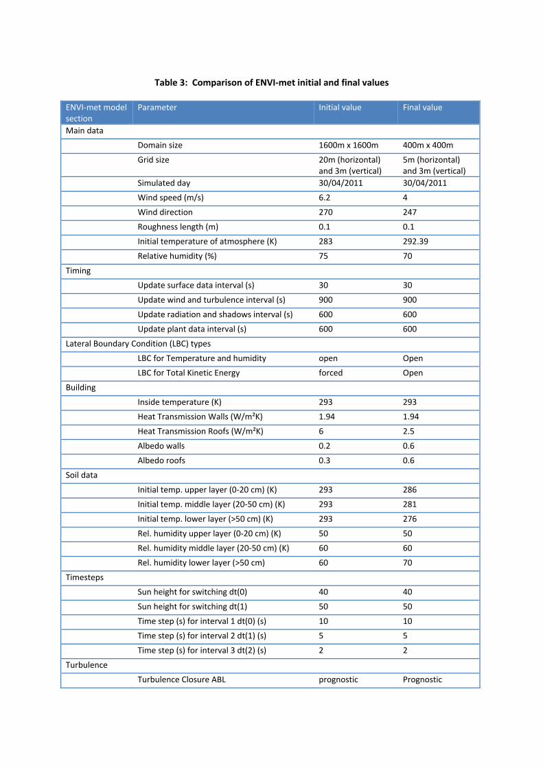
Table 3: Comparison of ENVI‐met initial and final values

ENVI‐met model section

Parameter Initial value Final value

Main data

Domain size 1600m x 1600m 400m x 400m

Grid size 20m (horizontal) and 3m (vertical)

5m (horizontal) and 3m (vertical)

Simulated day 30/04/2011 30/04/2011

Wind speed (m/s) 6.2 4

Wind direction 270 247

Roughness length (m) 0.1 0.1

Initial temperature of atmosphere (K) 283 292.39

Relative humidity (%) 75 70

Timing

Update surface data interval (s) 30 30

Update wind and turbulence interval (s) 900 900

Update radiation and shadows interval (s) 600 600

Update plant data interval (s) 600 600

Lateral Boundary Condition (LBC) types

LBC for Temperature and humidity open Open

LBC for Total Kinetic Energy forced Open

Building

Inside temperature (K) 293 293

Heat Transmission Walls (W/m²K) 1.94 1.94

Heat Transmission Roofs (W/m²K) 6 2.5

Albedo walls 0.2 0.6

Albedo roofs 0.3 0.6

Soil data

Initial temp. upper layer (0‐20 cm) (K) 293 286

Initial temp. middle layer (20‐50 cm) (K) 293 281

Initial temp. lower layer (>50 cm) (K) 293 276

Rel. humidity upper layer (0‐20 cm) (K) 50 50

Rel. humidity middle layer (20‐50 cm) (K) 60 60

Rel. humidity lower layer (>50 cm) 60 70

Timesteps

Sun height for switching dt(0) 40 40

Sun height for switching dt(1) 50 50

Time step (s) for interval 1 dt(0) (s) 10 10



Turbulence

Turbulence Closure ABL prognostic Prognostic

Turbulence Closure 3D Model prognostic Prognostic

Upper Boundary for e‐epsilon closed Closed

Table 4: Range of air temperature changes across the simulated domains

Gla CC‐W Gla CC‐E Paisley Clyde Gateway

Wishaw Hamilton

< ‐1.00

‐1.00 to ‐0.75 0.2%

‐0.75 to ‐0.50 0.6% 0.1% 0.4%

‐0.50 to ‐0.25 0.3% 1.8% 1.9% 3.2% 2.6%

‐0.25 to 0.00 90.9% 81.0% 94.6% 93.3% 96.6% 95.9%

0.00 to +0.25 8.8% 19.0% 3.1% 4.1% 0.0% 1.1%

+0.25 to +0.50 0.5% 0.1%

+0.50 to +0.75 0.0%

+0.75 to +1.00

> +1.00

Table 5: Predicted Mean Vote (PMV) due to a 20% increase in green cover in 2050

Gla CC ‐ W Gla CC ‐ E Paisley Clyde Gateway

Wishaw Hamilton

< ‐2.0

‐2.0 to ‐1.5

‐1.5 to ‐1.0 0.7% 2.0%

‐1.0 to ‐0.5 7.7% 1.0% 1.4% 8.9%

‐0.5 to 0.0 4.9% 3.6% 31.1% 20.4% 11.9% 19.1%

0.0 to +0.5 31.8% 35.6% 12.5% 8.4% 9.2% 8.4%

+0.5 to 1.0 15.8% 15.4% 5.8% 3.9% 2.1% 5.4%

+1.0 to +1.5 0.6% 2.1% 15.3% 15.3% 9.6% 18.7%

+1.5 to +2.0 7.0% 6.8% 24.6% 44.2% 57.6% 34.9%

> 2.0 40.0% 36.6% 2.5% 6.8% 8.2% 2.6%

Table 6: ‘Best’ outcome in Predicted Mean Vote (PMV) in 2050

Gla CC ‐ W* Gla CC ‐ E* Paisley** Clyde Gateway**

Wishaw** Hamilton**

< ‐2.0

‐2.0 to ‐1.5

‐1.5 to ‐1.0 1.2% 0.1% 3.3%

‐1.0 to ‐0.5 0.0% 14.4% 8.1% 7.1% 18.2%

‐0.5 to 0.0 3.6% 5.2% 42.0% 36.1% 19.3% 29.7%

0.0 to +0.5 48.8% 42.9% 14.5% 6.2% 9.2% 8.0%

+0.5 to 1.0 33.6% 24.7% 6.9% 3.8% 4.0% 9.8%

+1.0 to +1.5

1.2% 1.5% 9.6% 14.7% 13.8% 14.8%

+1.5 to +2.0

3.6% 2.4% 10.6% 30.4% 44.1% 16.0%

> 2.0 9.2% 23.4% 0.8% 0.6% 2.5% 0.2% Notes: ‘Best’ PMV outcomes are reached as follows: * ‐ 20% increase in green cover with Tall buildings (two city centre sites) ** ‐ 100% increase in green cover (all the other four sites)

Table 7: Assumptions and calculation method to derive green infrastructure options for Gla CC‐W

Parameter Quantity Remarks

1 Current green cover 3.3% Measured from GIS maps

2 Total area of the simulation domain 160,000m2 400m x 400m

3 Available sidewalk 11.15% Measured from GIS maps (assumes average sidewalk = 2m wide)

4 Standard cover of a street tree 4m2

5 Distance between trees 6m Thus, each tree would ‘cover’ 12m2 of sidewalk

6 Total available sidewalk area 17,840m2 [2] × [3]

7 Possible No of street trees in domain

1,486 [6] ÷ ([5] × 2)

8 Total possible street tree cover 5,947m2 [7] × [4]

9 Possible street cover as a fraction of total domain area

3.72% [8] × 100 ÷ [2]

10 Current built cover 52.42% Measured from GIS maps

11 Usable building cover 40% Based on a visual inspection of domain area for buildings with flat roof

12 Total usable building area 33,549m2 [10] × [11] × [2]

13 Total usable building area as a fraction of domain

21% [12] ÷ [2]

14 Assumed average height of building 12m Based on visual inspection

15 Total No of block in domain 13 Based on visual inspection

16 Average block size 35m × 30m

17 Total available Façade area 10,140m2 [16] × [14] × [15]

18 Total usable façade area as a fraction of domain area

6.34% [17] × 100 ÷ [2]

Table 8: Alternative approaches to increasing green cover by 20% in Gla. CC‐W

Scenario Permeable vegetated area (m2)

Street trees (Nos.)

Intensive Roof

Garden (m2)

Extensive Roof

Garden (m2)

Green façade

1. A large park only 1,056

2. Street trees only 528

3. 50% of additional greenery in street tree, balance intensive roof garden

264 755

4. 50% of additional greenery in street tree, balance extensive roof garden

264 1,056

5. Mix of intensive (50%) and extensive (50%) roof garden

755 1,056

6. 50% of all ‘sun facing’ (i.e. South & West) façade covered façade green

1,268

ListofFigures

Figure 1: Quantification of land cover types

Figure 2: Detailed view of LCZ classes with built cover categories

Figure 3: Selected locations for model simulations

Figure 4: Three dimensional view of selected sites showing the built‐ and green‐cover

Figure 5: Glasgow city simulation sites (Note: Both Gla CC‐W and Gla CC‐E are included in this image)

Figure 6: Glasgow Clyde Gateway simulation site

Figure 7: Paisley simulation site

Figure 8: Wishaw simulation site

Figure 9: Hamilton simulation site

Figure 10a: Temperature profile comparison of measured (GCU Weather Station) and simulated (ENVI‐met) temperatures in Glasgow on 30 April 2011

Figure 10b: Scatter plot of ENVI‐met predicted and measured temperatures

Figure 11: Air temperature effect of green infrastructure – daytime

Figure 12: Air temperature effect of green infrastructure – night time

Figure 13: Average daily summertime effects

Figure 14: Average daily summertime temperature effect of green cover

Figure 15: Surface temperature effects at daytime

Figure 16: Surface temperature effects at nighttime

Figure 1: Detailed view of LCZ classes with built cover categories

Figure 2: Selected locations for model simulations

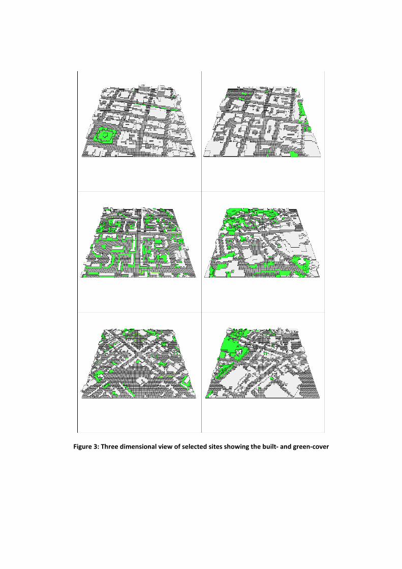
Figure 3: Three dimensional view of selected sites showing the built‐ and green‐cover

Top left: Glasgow City Centre west; Top right: Glasgow City Centre east

Middle left: Glasgow Clyde Gateway; Middle right: Paisley

Bottom left: Wishaw; Bottom right: Hamilton

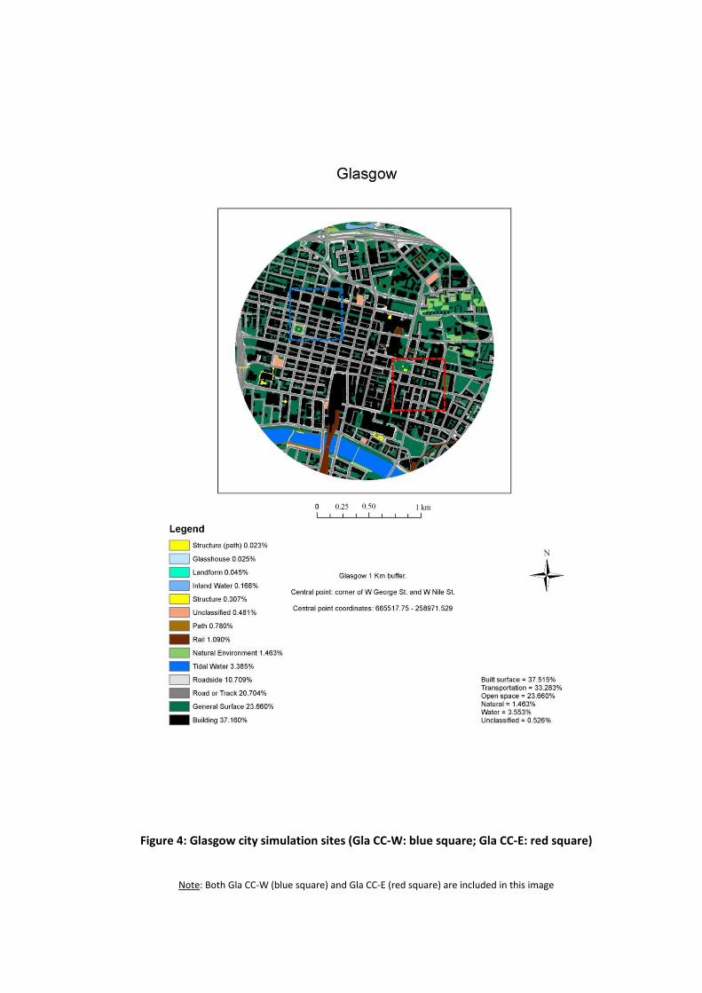
Figure 4: Glasgow city simulation sites (Gla CC‐W: blue square; Gla CC‐E: red square)

Note: Both Gla CC‐W (blue square) and Gla CC‐E (red square) are included in this image

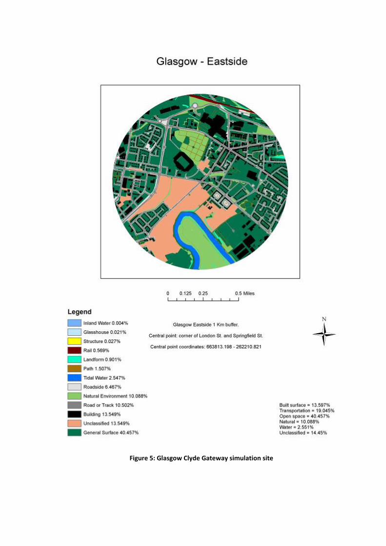
Figure 5: Glasgow Clyde Gateway simulation site

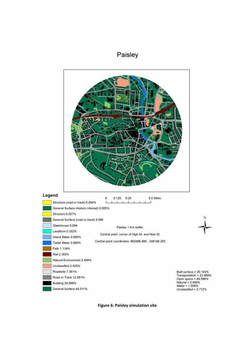
Figure 6: Paisley simulation site

Figure 7: Wishaw simulation site

Figure 8: Hamilton simulation site

Figure 9: Comparison of measured (GCU Weather Station) and simulated (ENVI‐met) temperatures

in Glasgow on 30 April 2011

Figure 10: Air temperature effect of green infrastructure – daytime

Notes: The slight increase in temperature at Glasgow CC‐E is an artefact of the location of the changes in green cover relative to the point for which the data is plotted in the figure above. An area averaged change in temperature, as detailed in Table 2 is more representative of the cooling effect in the entire simulated domain area.

Figure 11: Air temperature effect of green infrastructure – night time

Figure 12: Average daily summertime effects

Figure 13: Average daily summertime temperature effect of green cover

Fig 14: Surface temperature effects at daytime

Fig 15: Surface temperature effects at nighttime

Published in - Glasgow Caledonian...

Documents

Transcript of Published in - Glasgow Caledonian...