NAT L INST. OF STAND S TECH RT.C.

A111D3 bT3m5

PUBLICATIONS

Use of NISTStandard Reference

Materials for Decisions on'

Performance of Analytical

Chemical Methods andLaboratories

NIST Special

Publication 829

CAC Quality Assurance Task Group:

D. Becker, R. Christensen,

L. Currie, B. Diamondstone, K, Eberhardt,

T. Gills, H. Hertz, G. Klouda, J. Moody,

R. Parris, R. Schaffer, E. Steel, J. Taylor,

R. Walters, and R. Zeisler

S. Department of Commerce^ ^chnology Administration

itional Institute of Standards and Technology#829

1992

C.2

NATIONAL OF STANDARDS ft

^ . ULOItYt Research Information Center

1^ Gaithersburg, MD 20899..

DATE DUE

Demco, Inc. 36-298

NIST Special Publication 829

Use of NIST Standard Reference

Materials for Decisions on

Performance of Analytical Chemical

Methods and Laboratories

CAC Quality Assurance Task Group:

D. Becker, R. Christensen, L. Currie,

B. Diamondstone, K. Eberhardt, T. Gills,

H. Hertz, G. Klouda, J. Moody, R. Parris,

R. Schaffer, E. Steel, J. Taylor, R. Watters,

and R. 2Leisler

Chemical Science and Technology Laboratory

National Institute of Standards and Technology

Gaithersburg, MD 20899

January 1992

U.S. Department of CommerceRobert A. Mosbacher, Secretary

Technology Administration

Robert M. White, Under Secretary for Technology

National Institute of Standards and Technology

John W. Lyons, Director

National Institute of Standards U.S. Government Printing Office

and Technology Washington: 1992

Special Publication 829

Natl. Inst. Stand. Techno!.

Spec. Publ. 829

30 pages (Jan. 1992)

CODEN: NSPUE2

For sale by the Superintendent

of DocumentsU.S. Government Printing Office

Washington, DC 20402

I

USE OF NIST STANDARD REFERENCE MATERIALS FOR DECISIONS ONPERFORMANCE OF ANALYTICAL CHEMICAL METHODS AND LABORATORIES

Table of Contents

A. INTRODUCTION 1

B. APPROPRIATE SRM 1

C. STATISTICAL CONTROL 1

D. DETECTION OF BIAS 2

Dl . Planning the experiment: bias detection limit vs.

number of replicates 2

D2 . Testing the hypothesis of "no bias": experimental results 6

D3 . The treatment of SRM uncertainty 7

E. APPLICATIONS 11

El. Establishing statistical control of the analytical 12

measurement process

E2 . Tests for analytical measurement bias 14

E3 . Tests for analytical measurement acceptability 17

E4. Tests for single measurements ' 20

F . REFERENCES 22

G. APPENDIX 25

Gl. Percentiles of the t distribution 25

G2. List of Symbols 26

iii

USE OF NIST STANDARD REFERENCE MATERIALS FOR DECISIONS ONPERFORMANCE OF ANALYTICAL CHEMICAL METHODS AND LABORATORIES

A. INTRODUCTION

NIST Standard Reference Materials (SRMs) are used extensively for the

evaluation of analytical methods and laboratory performance. The generalprinciples of SRM use and the statistical tools useful for interpreting suchmeasurements are discussed in NBS Special Publication 260-100 [1]. The presentdocument describes specific guidelines and applications. Statistical guidanceis essential when developing a protocol for a specific measurement program andfor interpreting measurement data. The statistical methods outlined in thisdocument and in reference [1] are more completely discussed with their relatedapplications and assumptions in reference [2]

.

The following discussion is based on the use of an appropriate SRM to evaluateanalytical methods and laboratory performance.

B. APPROPRIATE SRM

SRMs used for the applications that follow should meet the followingrequirements to the extent possible:

1) Reasonable matrix match with the samples customarily analyzed,2) Reasonable match of analyte concentration(s)

,

3) Uncertainty of certified concentrations should be small with respectto the requisite uncertainty for the intended use.

It is virtually impossible for SRMs to exactly match the compositions oflaboratory samples, and the SRM uncertainty may not be negligible in someapplications. Accordingly, professional judgment and analytical expertise areneeded in the selection of the most appropriate SRM. In most cases, somecompromises will be inevitable. Notwithstanding these limitations, the use ofSRMs is considered to be one of the best available approaches for decisions onthe accuracy of measurement data. Specific directions for use, such as theamount of sample, the specimen treatment, and other analysis protocols aregiven on the SRM certificate. Unless these directions are followed explicitly,performance judgments based on the certified concentrations of the SRM may notbe valid.

C. STATISTICAL CONTROL

The chemical measurement process (CMP) to be evaluated or used must be in a

state of statistical control at the time any definitive measurements are made.That is, the measurement process must be stable and capable of producing a

limiting mean (n) and a fixed standard deviation (a) . While this can never berigorously demonstrated, there should be no reasonable doubt that control hasbeen achieved [3]. Furthermore, the standard deviation should be reasonablysmall with respect to any level of bias that is of concern. It is difficult to

detect a bias smaller than the standard deviation, without imposing majordemands on system long- terra stability and requiring large numbers of

1

replicates. Also, it is impossible to achieve a bias detection limit smallerthan twice the uncertainty of the standard reference material used (see sec.

D3) .

D. DETECTION OF BIAS*

If the uncertainty in the certified concentration of an SRM (for a givenanalyte) is negligible compared to the level of bias to be detected, the biasof a CMP may be estimated as the difference between the sample mean obtained byanalyzing the SRM using the CMP and the SElM's certified concentration.Knowledge of the standard deviation of the CMP permits one to: (a) determinethe relation between the number of replicates and the minimum detectablebias -- necessary for designing (planning) the experiment; and (b) test forbias and/or estimate a confidence interval for bias, given an experimental(mean) result. See reference [2] for a general discussion of these concepts.

Dl . Planning the experiment: bias detection limit (A^ ) vs. number ofreplicates

The objective of the first (planning) phase is to assure that thestatistical (t) test for bias has adequate "power" to detect the level ofbias considered important. That is, if the test for bias is made at the5% significance level (a = 0.05), we wish to have a 95% chance ofdetecting an absolute difference, Ap , between a measured mean and a "true"value (y8 = risk of false negative, and 1-^ = 0.95 = power of the test).It can be shown [4] that

~ (^l-ct/2 + ^i-fi)

where ti-a/2 is the 2-sided Student's t, ti_^ is the 1-sided Student's t,

o is the standard deviation, and n is the number of independentreplicates. Equation (1) yields direct values for Ap or a, given n; butan iterative solution is generally required to calculate n, given Ap anda, since the t's depend on n. Alternatively, the adjustment described in

the first footnote to table 1 can be used in lieu of iteration.

For large n or known a, t — z, the normal deviate, so Ap — (1.960 +

1.645) a/Jn for a = y8 = 0.05. In this case,

n > (3.605 a/Ap;2 = 13(a/Ap;2 = 13/^2 {2}

where d = Ap/a, the ratio of the bias to be detected to the measurementstandard deviation.

Thus, at least 13 replicates are required to detect bias equal to the

standard deviation. Stated differently, the standard error of the meanmust be smaller than the bias to be detected by at least a factor of 3.6.

See the Appendix for a list of s3nmbols and a table of the t distribution.

2

Dla. Tabulated niunbers of independent replicates (n)

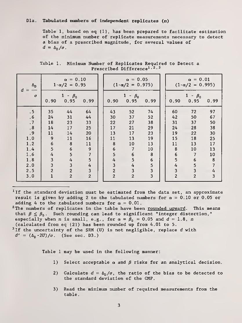
Table 1, based on eq {1}, has been prepared to facilitate estimationof the minimum number of replicate measurements necessary to detecta bias of a prescribed magnitude, for several values ofd = An/a.

Table 1 . Minimum Number of Replicates Required to Detect aPrescribed Difference^ .2,3

Q = 0. 10

Ad 1--a/2 = 0. 95

d -

a 1 - h0.90 0.95 0.99

.5 35 44 64

.6 24 31 44

.7 18 23 33

.8 14 17 25

.9 11 14 20

1.0 9 11 16

1.2 6 8 11

1.4 5 6 9

1.6 4 5 7

1.8 3 4 5

2.0 3 3 4

2.5 2 2 3

3.0 1 2 2

a = 0. 05

(1 -a/2 = 0. 975)

1 - )9o

0.90 0.95 0.99

43 52 74

30 37 52

22 27 38

17 21 29

13 17 23

11 13 19

8 10 13

6 7 10

5 6 8

4 5 6

3 4 5

2 3 3

2 2 3

a = 0 01

(1 -a/2 = 0 995)

1 - /So

0.90 0.95 0.99

60 72 97

42 50 67

31 37 50

24 28 38

19 22 30

15 18 25

11 13 17

8 10 13

6 7 10

5 6 8

4 5 7

3 3 4

2 2 3

^If the standard deviation must be estimated from the data set, an approximateresult is given by adding 2 to the tabulated numbers for a = 0.10 or 0.05 oradding 4 to the tabulated numbers for a = 0.01.

^The numbers of replicates in the table have been rounded upward . This meansthat < . Such rounding can lead to significant "integer distortion,"especially when n is small, e.g., for a = = 0.05 and d = 1.8, n(calculated from eq {2)) has been rounded up from 4.01 to 5.

•^If the uncertainty of the SRM (U) is not negligible, replace d withd' = (LQ-2U)/a. (See sec. D3.)

Table 1 may be used in the following manner:

1) Select acceptable a and risks for an analytical decision.

2) Calculate d = h^/a , the ratio of the bias to be detected to

the standard deviation of the CMP.

3) Read the minimum number of required measurements from the

table

.

3

Note that the nvimber in step 3 above should be increased by 2 to 4

if the standard deviation has not already been evaluated with areasonable number of degrees of freedom, say > 30, but must beestimated from the data set used for bias detection. (The firstfootnote to table 1 indicates the appropriate increments to n.)

The values for Aq and a may be absolute values or relative values(e.g., relative error and relative standard deviation), providedboth are on the same basis.

Another use of the table is in the estimation of the risk oferroneous decisions on bias detection, based on a limited number ofmeasurements. As an example, consider the case in which d = 1.0 andthe feasible number of measurements is limited to n = 10. Theclosest combination of a. and risks found in the table is a = )8

=

0.10. If the precision of the CMP could be improved by 20%, so thatd = 1.2, the risks based on 10 replicates would be decreased to a =

= 0.05.

From inspection of eq (2) and table 1, it is clear that the minimumnumber of replicates, n, varies as 1/d^ . Taking the case for a-

known and a = = 0.05, we see that duplicate measurements sufficeif Ap > 2.5 a, but as noted above, 13 measurements are required whenAj) = a.

EXAMPLES

SRM 2704, Buffalo River Sediment, is used to test a method for the

determination of Si. The Si certified concentration is 29.08 ± 0.13 wt%(Xq ± U) . (Note that the SRM uncertainty U is ignored in these examples,and that a and ^ axe each taken equal to 0.05.)

Planning the experiment (Ap,given n, and vice versa)

If the CMP to be evaluated has an imprecision (c) of 2.5 wt% Si, what is

the minimum detectable bias (Aj,) for a = ^ = Q .05 for a given number of

replicates (n)?

1) a-estimated, n = 5 (df=5-l=4):

(^0.975 ^^0.95)^

Ad s (Eq {1})

Jn

{l.lie + 2.132)2.5= = 5.49 wt% Si

75

4

2) a-known, any n:

(^0 .975 ^0.95)*^

Ad = (Eq {1})

Jn

(1.960 + 1.645)2.5 9.01

Jn Jn

Comparative results:

Minimum detectable bias, Ap

(wt% Si)

n = 5 n = 25

a-estimated 5.49 1.89

a-known 4.03 1.80

3) Approximation, using table 1:

For n = 25 (a-known), interpolation gives d ~ 0.73. Thus,

Ad = ad = (2.5) (0.73) = 1.8 wt%.

For n = 25 (a-estimated), n' - n-2 must be used. Interpolatingfor 23 replicates gives d ~ 0.77. Thus,

Ap (2.5) (0.77) = 1.9 wt%.

How many replicates are required to detect a bias (Ap) of 5% of thecertified concentration using a spectrometrie method which has a a =2.5 wt%? (Ad = 0.05 x 29.08 = 1.454 wt%)

1) a-estimated: n >

Ad

(Eq (1) transformed)

> 41 (by iteration)

Note that convergence is extremely rapid, since n must be aninteger. In fact, the correct answer can generally be obtained byadding 1 or 2 replicates to the number calculated for the "a-known"case. Iteration is necessary because Student's t depends on the

number of replicates, n, through the degrees of freedom(df = n - 1)

.

5

2) a-known: n ~ 13(a/hj^)^ (Eq {2})

» 13(2.5/1.454)2 38.4

Rounding up, n should be 39, since replicates are discrete.

3) Approximate results may be obtained "by inspection" using table

1 4541, and the value for d = Ap/a =

^ ^= 0.582. n (tr-known) thus

lies between 52 (d = 0.50) and 37 (d = 0.60). Crude inter-polation yields n = 40 (a-known) and n = 42 (a-estimated fromthe experiment)

.

D2. Testing the hypothesis of "no bias": experimental results

The objective of the second phase is to apply the t-test to the nullhypothesis ("no bias"), given an experimental result: x, s, n. Thecritical value (A^ ) for testing for bias is

= ^i-a/z^/^- (3)

The estimate of_bias (K) is the difference between the observed meanconcentration (x) and the certified concentration of the analyte in theSRM (xo).

K = X - Xq {4}

If the absolute value of the estimated bias does not exceed A^ , the nullhypothesis is not rejected; i.e., bias is not detected.* This does notmean that the CMP is unbiased , but that whatever bias might be present is

"acceptable," provided that n is large enough to ensure that the test hasadequate power (see above)

.

A complementary treatment of the experimental outcome is to compute a

confidence inteirval (CI) for the bias. If the interval spans zero, any

bias that is present is statistically insignificant ^ another way of

phrasing the t-test [5]. Thus,

CI = K ± t^.^i^s/J^ . {5}

In a properly designed experiment, the confidence limits for an unbiased

CMP are considerably smaller (in absolute value) than any bias of

practical importance

.

*The reader may have noticed that the critical value (A^ ) tends to be smaller

than the detection limit, Ap . This occurs because the detection limit is

calculated to meet the stringent requirement that the estimated bias (A) has

high probability (1-/9) of exceeding the critical value (Ac) whenever the true

bias is at the detection limit (Ap). True bias somewhat below the detection

limit may also be detected (i.e., yield data with A greater than the critical

value) but will do so with correspondingly lower probability (lower than 1-^).

6

EXAMPLES

Testing the hypothesis: experimental results

Suppose an experimental result of 27.32 wt% Si with a standard deviationof 2.64 wt% is obtained by a CMP for SRM 2704:

X = 27.32 wt%s = 2.64 wt%

A = X - Xo (Eq {4))= 27.32 - 29.08 = -1.76 wt%

The critical value is

Ac = gy^s/J^ (Eq {3})

(if a is known, use Zq gy^ajn)

If there were 5 replicates, is bias detected?

For n = 5, to 975 = 2.776: Ac = 2.776(2.64/75) =3.28 wt%

|A| < Ac , so bias is not detected at the 0.05significance level.

Bias Uncertainty Interval:

A confidence interval for the bias of CMP is given by:

CI = K ± to.975s/7Ji (Eq {5})

= -1.76 ± 2.776(2.64/75)

= from -5.04 to 1.52 wt% (includes 0)

If n is increased to 25, Aj. is reduced to 1.09 wt% Si (eq {3}). In thiscase, \A\ > A^ , so bias is. detected. Its uncertainty interval comprises -

2.85 to -0.67 wt% Si (eq (5)).

D3. The treatment of SRM uncertainty

Thus far we have assumed negligible uncertainty (17) for the certifiedconcentration of the SRM. If that is not the case, we must take intoaccount the magnitude of U in testing for bias and constructing confidenceintervals for bias. Unfortunately, this cannot be done in a rigorousfashion unless the estimated value (xq ) for the SRM is truly a random

variable ^ i.e., a quantity derived strictly from random error ^ and the

SRM is recertified each time we wish to make the test. Generally, neitherof these conditions is fulfilled: (1) the SRM is certified once . not eachtime a test for bias is made; (2) U frequently involves systematic

7

components in addition to random measurement error, and the method usedfor estimating and combining such components is not always the same, oreven known to the user. (The one realistic case in which the SRM estimatemay be treated as a random variable is when the primary source of error is

within-sample heterogeneity for the SRM issued to the user. In this case,the actual concentration varies randomly each time the SRM is sampled.)

Two procedures may be followed: (1) treat the SEIM interval as bounds forfixed (systematic) error [6]; (2) treat the SRM uncertainty interval as a

random error confidence interval, and "propagate" the correspondingvariance [7]. The first, which is discussed below, is clearly the moreconservative approach and the one we recommend. The second approach is

not discussed here.

To illustrate, let us assume that certificate information is given in theform

Xq ± where Xq is the certified concentration, and U representsthe assigned (symmetric) uncertainty bounds.

Note that Xg is not necessarily the true value of the analyteconcentration, but rather the best estimate of the true value based onmeasurement. Also, note that U need not be sjnaametric. This presentationwill not, however, treat asymmetric limits, nor non-normal random error.

Taking the lower and upper bounds for the SRM uncertainty to be syrmnetric

(±[/) , we now treat [/ as a fixed offset that increases both the detectionlimit for bias, and the uncertainty interval for experimentally estimatedbias. The original expressions given in sections Dl and D2 are modifiedas follows.

Bias Detection Limit: Ap = (^i-a/2 ^i-p^ (^/J^ + 2U {6}

Critical Value: = t^-ai2^/J^ + U (7)

Bias UncertaintyInterval:* UI = K ± (t^.^,^s/Jn + \J) (8)

Illustrations which take SRM uncertainty into account are given below.

Even without numerical examples, however, it is useful to consider the

limiting cases: When U is small compared to the standard error {a/Jn) , it

may be ignored and the above expressions revert to the earlier ones. WhenU is large compared to the standard error, both the critical value and

bias uncertainty limit approach U; and the bias detection limit approaches

2U . For further information on the detection of bias, and the effect of

systematic error on detection limits, see reference [8].

*The uncertainty interval {UI) is introduced here as a generalization of a

statistical confidence interval (CI) . This is necessary because the concept

of a rigorous confidence level, 1-a, is inapplicable in the presence of

non-statistical systematic error bounds. If the systematic error bounds are

negligible or treated as random, UI and CI are identical.

8

EXAMPLES

The certified concentration for Si in SRM 2704, Buffalo River Sediment, is

29.08 ± 0.13 wt% (Xq ± 17) .

We shall assume that the SRM is used to evaluate the bias of a gravimetricmethod having a standard deviation for silicon of a = 0.20 wt% . Thus theuncertainty interval for the SRM cannot be ignored. (As before, we shalltake a = ^ = 0.05.)

Planning the experiment

Given the imprecision (a) of 0.20 vt% for the CMP to be evaluated, what isthe minimum detectable bias (Aq) for a given number of replicates (n)?

1) a-estimated, 27 = 5: .

= (2.776 + 2. 132) (0.20/75) + 2(0.13) = 0.699 wt% Si

2) a-known, any n:

C^O.9 7 5 + ^0.95>> ^/-f^ + (Eq (6))

= (1.960 + 1.645)(0.20/yJ^) + 2(0.13) = 0.12l/J^ + 0.26

Comparative results

:

Minimum detectable bias,(wt% Si)

n = 5 n = 25

a-estimated 0.699 0.411

a-known 0.582 0.404

3) Approximation, using table 1*

For 27 = 25 (a-known), interpolation gives d' ~ 0.73. Thus,

Ad = ad' + 2U ^ (0.20)(0.73) + 2(0.13) = 0.406 wt%

For n = 25 (a-estimated), n' = n-2 must be used. Interpolatingfor 23 replicates gives d' -0.77. Thus,

Note that allowance for systematic error bounds requires that d be replaced byd' = (Ajj-2U) /a for use with table 1. This transformation follows directlyfrom the defining eqs (1) and (6).

9

Ad = ad' + 2U ^ (0.20)(0.77) + 2(0.13) = 0.414%

Thus, when as many as 25 replicates are available for estimatinga, the bias detection limit is nearly as small as for the casea -known.

How many replicates are required to detect a bias of 0.22 wt%?

Bias Detection Limit:

^^0 .9 7 5 + ^0.95 ; a/Jn + 2U (Eq (6))

> 2U = 0.26 wt%

The smallest achievable bias detection limit (Ap ) is 2U . Therefore, abias detection limit of 0.22 wt% cannot be achieved regardless of thenumber of replicates. Corresponding to the minimum value for Aq of2U = .26%, the minimum critical value, A^. , is U = 0.13% (see footnote onpage 6)

.

How many replicates are required to detect a bias equivalent to 1.5% ofthe certified concentration, using the gravimetric method having astandard deviation (a) of 0.20 wt% Si?

Ad = 29.08 (0.015) = 0.4362 wt% Si

1) a-known:

(^0 .97 5 ^0.95n >

Aq - 2U(Eq (6) transformed)

' (1.960 + 1.645)0.20

0.4362 - 2(0.13)

= 16.74

Since replicates are discrete, the minimum value for n becomes17.

2) <7-estimated:

(^-0.975 ^0.95)*n >

Ad - 2U(Eq (6) transformed)

(^0.975 ^0.95)^*^

0.4362 - 2(0.13)^

10

= 19 (by iteration)

3) Approximation, using table 1:

Ad - 2U 0.4362 - 2(0.13)First calculate d' = = = 0.881

a 0.20n (£T-known) thus lies between 17 (d'=0.9) and 21 (d'=0.8).Crude interpolation yields n = 18 (<7-known) and n = 20 (cr-

estimated) .

Testing the hypothesis: experimental results

Experimental results examined for bias

Suppose that a more precise method of analysis were used to obtain the

following results:

X = 29.40 wt%

s = 0.17 wt%

A = X - Xq (Eq (4))

K = 29.40 - 29.08 = 0.32 wt% Si

If there were 5 replicates, is bias detected?

n = 5: Ac = Cfj gy^s/Jn + U

= 2.776(0.17/75)+ 0.13 = 0.341 wt% Si

|A| < Aj. so bias is not detected at the 0.05significance level.

Bias Uncertainty Interval:

UI = A ± (Cq gy^S/J^ + U)

. = 0.32 ± (2.776(0.17/75) + 0.13)

= from -0.021 to 0.661 wt% Si

If n is increased to 25, A^ is reduced to 0.200 wt% Si (eq (7)). Inthis case,|A| > A^ , so bias is detected. Its uncertainty intervalcomprises 0.120 to 0.520 wt% Si (eq {8)).

E. APPLICATIONS

The most frequent applications of SRMs for the evaluation of measurementprocesses relate to the following questions:

(Eq {7})

(Eq (8))

11

1) Are the analytical results produced by a laboratory understatistical control? (El)

2) Are the analytical results biased? (E2)

2a) Is the method biased? (E2a)

2b) When the method is known to be unbiased, are the results from aparticular laboratory biased? (E2b)

2c) When the method bias is not known, are the results from a particularlaboratory biased? (E2c)

3) Are the analytical results acceptable, even if they exhibit somebias? (E3)

3a) Is the mean result of a set of replicate measurements acceptable?(E3a)

3b) Does an acceptable percentage of results fall within specifiedlimits of a measurement program? (E3b)

4) Are the analytical results biased or unacceptable, based on testswith only a single measurement? (E4)

Establishing statistical control of the analytical measurement process

It is recommended that SRMs be used in combination with control charts

[1,3] for systematic monitoring of a measuring system for attainment andmaintenance of statistical control. General guidance for this purpose is

contained in sections 3.3 and 3.4 of reference [1]. When it is notfeasible for a laboratory to use SRMs for this purpose on a regular basis(due to cost considerations, for example), a laboratory may use its own orother control samples on a routine basis, and on a less frequent basis,measure an SRM to verify the reliability of the control data obtained withother materials [3].

EXAMPLE

Over a period of 8 years, SRM 909, Human Serum, has been used at NIST as a

control material to monitor the performance of a definitive isotope

dilution method for measuring cholesterol in samples of human serum. Data

from 15 sets (four measurements per set) have been plotted on control

charts, figures 1 and 2, using methods described in reference [3].

The first control chart (fig. 1) is used to test the measurement process

for stability of the mean, and is a plot of the difference of the mean of

four measurements from the certified concentration for cholesterol in SRM

909. The upper and lower control limits (UCL, LCL) are "3-sigma" control

limits calculated from the standard deviation of the differences of the

means of the first 12 sets from the certified concentration. The upper

12

0.03

0.02 - - UCL

UWL

0.01

Mean -

Certified Value

(mmol/L)

0 --

-0.01 --LWL

-0.02

LCL

H H H \1

2 3 4 5 6 7 S 9 10 11 12 13 14 15

iVIeasurement Set Number

Figure 1. Control Charts to Test for Stability of the Mean

0.05

0.05

0.04

0.04

0.03

Range of Set of 4

l\/leasurements o.03

(mmoi/L)

0.02

0.02

0.01

0.01 --

0.00

UCL

UWL

H h—H H H h

5 6 7 a 9 10 11

iVIeasurement Set Number

H h

12 13 14 15

Figure 2. Control Chart to Test Precision of CMP

13

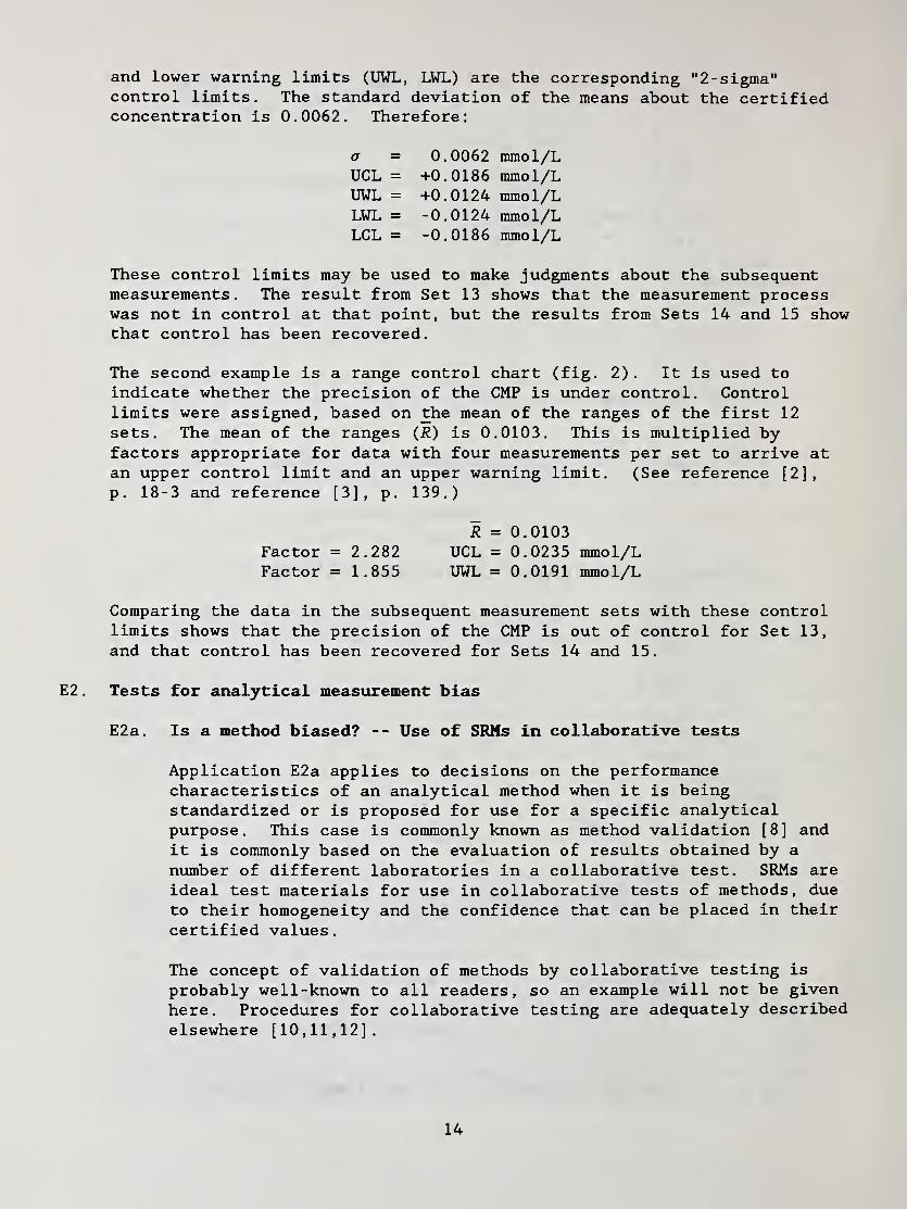
and lower warning limits (UWL, LWL) are the corresponding "2-sigma"control limits. The standard deviation of the means about the certifiedconcentration is 0.0062. Therefore:

a = 0.0062 mmol/LUCL = +0.0186 mmol/LUWL = +0.0124 mmol/LLWL = -0.0124 mmol/LLCL = -0.0186 mmol/L

These control limits may be used to make judgments about the subsequentmeasurements. The result from Set 13 shows that the measurement processwas not in control at that point, but the results from Sets 14 and 15 showthat control has been recovered.

The second example is a range control chart (fig. 2). It is used to

indicate whether the precision of the CMP is under control. Controllimits were assigned, based on the mean of the ranges of the first 12

sets. The mean of the ranges (J?) is 0.0103. This is multiplied byfactors appropriate for data with four measurements per set to arrive atan upper control limit and an upper warning limit. (See reference [2],

p. 18-3 and reference [3], p. 139.)

Comparing the data in the subsequent measurement sets with these controllimits shows that the precision of the CMP is out of control for Set 13,

and that control has been recovered for Sets 14 and 15.

Tests for analytical measurement bias

E2a. Is a method biased? -- Use of SRMs in collaborative tests

Application E2a applies to decisions on the performancecharacteristics of an analytical method when it is beingstandardized or is proposed for use for a specific analyticalpurpose. This case is commonly known as method validation [8] andit is commonly based on the evaluation of results obtained by a

number of different laboratories in a collaborative test. SRMs are

ideal test materials for use in collaborative tests of methods, due

to their homogeneity and the confidence that can be placed in their

certified values.

The concept of validation of methods by collaborative testing is

probably well-known to all readers, so an example will not be givenhere. Procedures for collaborative testing are adequately describedelsewhere [10,11,12].

FactorFactor

= 2.282= 1.855

RUCLUWL

0.01030.0235 mmol/L0.0191 mmol/L

14

E2b. Does a laboratory tising an unbiased method produce unbiased data?

Application E2b applies to decisions that every laboratory shouldaddress whenever it uses methods for the first time or in a newapplication; namely, the demonstration of its ability to use amethod that has been previously validated [9]

.

The procedure recommended consists of making a set of measurementsand comparing the mean value with the certified value of thereference material. If the measured value does not differsignificantly from the certified value, it may be concluded that thedata are unbiased. Since the method used has been previouslyestablished to be unbiased at a given level of significance, anybias that is discovered can be attributed to laboratory performance.The laboratory then needs to investigate and correct the sources ofits bias, if the method is to be used. Tests should be made atappropriate analyte levels within the range of measurement.

EXAMPLE

Aluminum was determined in SRM 1646, Estuarine Sediment, usingInductively Coupled Plasma Emission Spectrometry. Eight independentmeasurements were made, which resulted in a mean value of 5.86 wt%Al and a standard deviation of 0.30 wt% . The certifiedconcentration and its uncertainty for Al in SRM 1646 are 6.25 ± 0.20wt%

.

X = 5.86 wt%

s = 0.30 wt%

Xq = 6.25 wt%

U = 0.20 wt%

A = X - Xq (Eq (4))

= 5.86 - 6.25 = -0.39 wt% Al

Ac = to. 9 7 5 VTn + U (Eq (7))

= 2.365 (0.30/78) + 0.20 = 0.45 wt% Al

|A| < so bias is not detected at the 0.05significance level.

15

Bias Uncertainty Interval:

UI = K ± (to 97 55/7^^ + U) (Eq {8})

= -0.39 ± {2.365 (0.30/78) + 0.20)

= from -0.84 to +0.06 wt% Al

E2c. Does a laboratory using its own (xinvalidated) method produceunbiased data?

This case applies to situations in which a laboratory utilizesmethodology that has not been validated by others, and desires toknow whether the data produced are unbiased. There are two possiblesources of bias in the analytical results: (1) bias inherent in themethod, and (2) bias resulting from the laboratory's use of themethod.

The procedure described in Application E2a may be followed. If theobserved difference between the mean of the experimental data andthe certified concentration of the SRM is not significant, one mayconclude, within the significance level of the statistical test,

that the combination of both the method and the laboratory producesunbiased data. If bias is detected, one is uncertain whether thisbias is due to source (1), (2), or a combination of the abovecauses. A research investigation will ordinarily be required to

answer these questions. One may devise appropriate tests to

systematically investigate contributions to bias from sources suchas calibration problems, blank corrections, contamination, andlosses [3]. Likewise, one may investigate the various steps in the

method for their contributions to bias. Comparison of the testresults with those obtained using a reference or definitive methodis another way to evaluate bias [3] , and does not involve use of anSRM.

EXAMPLE

Two gas chromatographic methods , which differed only in the internalstandard used, were evaluated for the determination of selectedpolycyclic aromatic hydrocarbons (PAH) in traffic tunnel particulatematerial. The following means and standard deviations were obtainedfrom six analyses of SRM 1650, Diesel Particulate Material, by each

method, for the listed PAH.

16

SRM 1650 - Diesel Particulate Material

Concentration, A»g/g

Method A Method BCertified

Concentration

± U

FluoranthenePyreneBenz [ a ] anthracene

56.6 7.2 65.2 7.3

53.4 8.4 61.6 9.25.1 2.4 5.8 2.7

51 ±448 ±46.5 ± 1.1

For each PAH result, the absolute difference between the mean andthe SRM certified concentration (A) was calculated. Then for a =

0.05, the critical value (A^.) was calculated using eq (7) (n = 6,

-0.975 = 2.571)

Method A Method B

K Ac K Ac

Fluoranthene 5.6 11.6 14.2 11.7Pyrene 5.4 12.8 13.6 13.7Benz [ a ] anthracene -1.4 3.6 -0.7 3.9

The determination of fluoranthene using Method B is biased at thesignificance level of the test. Because the methods differ only inthe internal standards used, the choice of internal standard inMethod B is considered to be inappropriate. For the other results,the absolute difference between the mean and the SRM certifiedconcentration is less than the critical value , so bias is notdetected. However, in the case of pyrene by Method B, the result is

on the borderline, so further investigation may be warranted.

Tests for analytical measiirement acceptability

Application E3 applies to decisions related to a laboratory's ownassessment of its analytical measurement capability and to the selectionand validation of laboratories to be used in a specific measurementprogram. Application E3a deals with bias in a measurement process;therefore, the population (or limiting) mean of a laboratory's resultsshould fall within the specified limits. In Application E3b , we areconcerned with individual results from a laboratory's measurement process;therefore, most of the population , i.e., a specified percentage, of a

laboratory's results should fall within the specified limits.

The difference between this situation and Application E2 is the concept of

"acceptability." The user of the data decides what limits of error in the

data are acceptable, based on practical considerations. Cost and benefitsare prime considerations when deciding what limits are acceptable. These

17

limits are generally larger than the uncertainties of the SRM and of themethod used and may often be considerably larger. This extra limit oferror (A) is added to the uncertainty bounds of the SRM so that theoverall acceptable range is Xq ± (U+A) . Equation {7} is then modified toyield the critical value for acceptability:

Ac = ^i-a/z s/Jn + (U+A) [9)

E3a. Does a laboratory using an unbiased or reference method produce apopulation mean result with acceptably small bias?

Application E3a deals with decisions on the acceptability of thepopulation mean of a laboratory's results which were produced usingan unbiased or reference method. The recommended procedure to beused is as follows:

1) Put specification limits around the certified concentration ofthe SRM to indicate the limits of bias considered to beacceptable. These limits should include the uncertaintyassigned to the certified concentration. Calculate thecritical value using eq (9).

2) Compare the difference between the analytical result and thecertified value with the critical value. If |a| < , thelaboratory is considered to be producing acceptable data.

Note that specification limits may be based on arbitrary decisionsor on the statistics of group performance in a collaborative test.

For example, they may represent the limits for values that 99% ofthe laboratories are expected to produce when using a methodcorrectly.

EXAMPLE

A laboratory used SRM 1173, a Ni-Cr-Mo-V steel, as a quality controlmaterial to check the acceptability of results for verifying that anunknown steel sample was of a similar alloy type. The elementdetermined was carbon, and the predetermined allowance for bias was

± 5% of the true value for the SRM in addition to the uncertainty in

the certified concentration. The certified concentration for carbon

in SRM 1173 is 0.423 ± 0.004 wt%. The limits of acceptability were

± 0.021 wt%. The mean value of four measurements was 0.400 wt% with

a standard deviation of 0.003 wt%.

X = 0.400 wt%

s = 0.003 wt%

Xq = 0.423 wt%

U = 0.004 wt%

18

A = 0.021 wt%

n = 4

= X - Xn (Eq (4))

= 0.400 - 0.423 = -0.023 wt% C

Ac = ti.„/2 s/J^ + (^-^A) (Eq {9})

= 3.182(0.003/A) + (0.004 + 0.021) = 0.030 wt% C

|A| < so unacceptable results are not detected at the

0.05 significance level (performance is deemedacceptable)

.

E3b. Does an acceptable percentage of a laboratory's results fall withinspecified limits?

Application E3b applies to decisions on the acceptability of resultsfrom an unbiased method or a test method in an ongoing measurementprogram, for example. Since the standard deviation of themeasurements is estimated from a limited sampling of the populationof measurements, a tolerance interval, which allows for the coverageof a specified percentage of this population at a certainprobability level, is computed.* The recommended procedure is:

1) Note the specification limits around the certifiedconcentration of the SRM which have been established for themeasurement program.

2) Compute the tolerance interval (TI) for the measurement processas the 2-sided tolerance interval for the population ofmeasurement results where 7 = 0.90, P = 0.90:

TI = x ± Ks (10)

*The tolerance interval approach presented presumes single observations whichare normally distributed. Tables are available for results which are means ofreplicates [13]. Alternative methods for evaluating CMP performance may beappropriate, such as: (a) "prediction intervals" (expected coverage toleranceintervals) [14], and (b) uncertainties comprising bounds (possibly asymmetric)for systematic and/or random error based on "expert judgment." If normalitycannot be assumed, a distribution- free approach may be applied, but at least

50 observations are required [15].

19

In the above equation, x and s denote the observed mean andstandard deviation based on n independent samples (measure-ments) , and K is the factor for the statistical toleranceinterval corresponding to the above choices for 7 and P, where7 is the probability that at least a proportion P of thepopulation of results will be included in the interval. Valuesfor K are obtained from statistical tables, such as intable A-6 of reference [2].

3) If the limits given by eq {10} lie within the specificationlimits, consider the CMP (for the given laboratory method) tobe performing "acceptably." Note that this comparison takesinto account possible bias and its uncertainty as well asrandom measurement error.

EXAMPLE

Assume that 10 measurements of methane in air (SRM 1658a), using a

specified, validated GC-FID method yield a mean of 1.038 /xmole

methane per mole air and an observed standard deviation of 0.052.In a table for 2-sided normal tolerance intervals for n = 10, 7 =

0.90, and P = 0.90, we find that K = 2.535. The tolerance intervalestimated for this CMP is thus:

X = 1.038 /xmol/mol

s = 0.052 /imol/mol

TI = X ± Ks (Eq (10))

= 1.038 ± 2.535(0.052)

= from 0.906 to 1.170 /xmol/mol

If the specification limits around the certified concentration rangefrom 0.900 to 1.100 /xmol/mol, the performance of this CMP (labora-tory method) must be judged "unacceptable," since the toleranceinterval does not lie totally within the specification limits.

Tests for single measurements

Application E4 applies to decisions regarding method validation orlaboratory performance when the ongoing measurement protocol results in a

single datum. In this case the standard deviation, s, must be establishedthrough experience with the measurement program which is often recordedusing a control chart. For decisions concerning bias, eq {6} is used with

the appropriate t value chosen for the number of degrees of freedom used

to estimate s. The value for n is 1 . For decisions concerningacceptability, eq {9} is used with the same provisions for n and df.

20

EXAMPLE

To illustrate, we return to the control chart example (see El.), involvingthe measurement of cholesterol in SRM 909, Human Serum. Over a period of8 years, 12 measurements of cholesterol in 1-gram samples of the controlmaterial were made. (For this example, we treat the mean value for a setof four determinations, as described in El, as a single measure-mentresult.) The standard deviation of a single measurement was 0.0062mmol/L, and the mean of the 12 measurements differed from the certi-fiedconcentration by an insignificant amount. The uncertainty of the

certified concentration for 1 gram of material is ± 0.014 mmol/L. Athirteenth measurement differed from the certified concentration by 0.029mmol/L. Does this measurement indicate bias?

s = 0.0062 mmol/L

n = 1

975~ 2.201 for 11 degrees of freedom

U = 0.014 mmol/L

= X - xo (Eq {4))

= 0.029 mmol/L

Ac = ^0.9 7 5 3/7^^ + U (Eq (7))

= 2.201(0.0062) + 0.014 = 0.0276 mmol/L

|A| > so an unacceptable result is detected at the0.05 significance level, and the thirteenthmeasurement is biased.

Decisions on measurement data such as those described above apply only to themeasurement system and measurement situations tested. Any extension of thedecisions to any other systems or situations will need to be justified.Because of the uncertainty of generalization, it is recommended that measure-ments made for validation of methods and qualification of laboratories shouldsimulate the expected analytical conditions as closely as possible. When a

variety of analytical conditions are to be expected (analyte levels and samplematrices) , the entire range of expected conditions should be tested. Thissubject is discussed further in section 6.4 of reference [1].

21

F. REFERENCES

[I] Taylor, J. K. , Standard Reference Materials: Handbook for SRM Users :

Natl. Bur. Stand. (U.S.) Spec. Publ. 260-100; U.S. Government PrintingOffice: Washington, DC, 1985.

[2] Natrella, M. G.,"Comparing materials or products with respect to average

performance," In Experimental Statistics : Natl. Bur. Stand. (U.S.)Handbook 91; U.S. Government Printing Office: Washington, DC, 1963;Chapter 3, pp. 3-1 to 3-42. (See also the collection of statisticaltables at the end of the Handbook.)

[3] Taylor, J. K.,Quality Assurance of Chemical Measurements : Lewis

Publishers: Chelsea, MI, 1987; Chapter 14.

[4] Currie, L. A., "Analyte and bias detection limits; approximations to thenon-central t distribution," Natl. Inst. Stand, and Technol. InternalReport; Gaithersburg, MD, September 1990 (In preparation).

[5] Natrella, M. G., "The relation between confidence intervals and tests ofsignificance," In Statistical Concepts and Procedures. PrecisionMeasurement and Calibration : Ku, H. H.

,Ed.; Natl. Bur. Stand. (U.S.)

Spec. Publ. 300, Vol. 1; U.S. Government Printing Office: Washington, DC,

1969; pp. 388-391.

[6] Eisenhart, C, , "Realistic evaluation of precision and accuracy ofinstrument calibration systems," J. Res. Natl. Bur. Stand. (U.S.) 1963,67C . 161.

[7] Colle, R. ; Karp, P., "Measurement uncertainties: Report of aninternational working group meeting," J. Res. Natl. Bur. Stand. (U.S.)

1987, 92, 243.

[8] Currie, L. A., "Detection: Overview of historical, societal, andtechnical issues," In Detection in Analytical Chemistry: Importance.Theory, and Practice : Currie, L. A., Ed.; ACS Symposium Series 361;

American Chemical Society: Washington, DC, 1988; Chapter 1.

[9] Taylor, J. K. , "Validation of analytical methods," Anal. Chem. 1983, 55,

600A-608A.

[10] Taylor, J. K. , "Role of collaborative and cooperative studies in the

evaluation of analytical methods," J. Assoc. Off. Anal. Chem. 1986, 69,

398-400.

[II] "Guidelines for collaborative study procedure to validate characteristicsof a method of analysis," J. Assoc. Off. Anal. Chem. 1989, 72, 694-704,

[12] ASTM E691, "Practice for conducting an interlabortory test program to

determine the precision of test methods," American Society for Testing and

Materials: Philadelphia, PA 19103.

22

[13] Eberhardt, K. E.;Mee, R. W.

;Reeve, C. P., "Computing factors for exact

two-sided tolerance limits for a normal distribution," Communications inStatistics 1989, 18, 397-413.

[14] Whitmore, G. A., "Prediction limits for a univariate normal distribution,"The American Statistician 1986, 40, 141-143.

[15] Natrella, M. G., "Tables A-30 and A-31: Distribution- free tolerancelimits," In Experimental Statistics : Natl. Bur. Stand. (U.S.) Handbook 91;

U. S, Government Printing Office: Washington, DC, 1963; pp. T-75 andT-76.

23

G. APPENDIX

Gl. Percentiles of the t distribution

(From reference [2] , table A-4)

df .60 .70 .80 ton.90 .95 .975 too.99 too.;.935

1 .325 .727 1.376 3.078 6.314 12.706 31.821 63.657

2 .289 .617 1.061 1.886 2.920 4.303 6.965 9.925

3 .277 .584 .978 1.638 2.353 3.182 4.541 5.841

4 .271 .569 .941 1.533 2.132 2.776 3.747 4.604

5 .267 .559 .920 1.476 2.015 2.571 3.365 4.032

o ceo.ooor\r\r>.90o 1 .440 1.943 AA'7 3.143 3.707

7 .263 .549 .896 1.415 1.895 2.365 2.998 o Ann3.499oo .262 .546 .889 1.397 1.860 o one2.306 o one2.896 o occ3.355

9 .261 .543 .883 1.383 1.833 2.262 2.821 3.250

10 .260 .542 .879 1.372 1.812 2.228 2.764 3.169

11 .260 .540 .876 1.363 1.796 2.201 2.718 3.106

12 .259 .539 .873 1.356 1.782 2.179 2.681 3.055

13 .259 .538 .870 1.350 1.771 2.160 2.650 3.012

14 .258 .537 .868 1.345 1.761 2.145 2.624 2.977

15 .258 .536 .866 1.341 1.753 2.131 2.602 2.947

16 .258 .535 .865 1.337 1.746 2.120 2.583 o no42.921

17 .257 .534 .863 1.333 1.740 2.1 10 2.567 o ono2.898

.257 .534 .862 1.330 4 70^1.734 2.101 o ceo2.552 O 070£.878

19 .257 coo.533 .861 1.32B 4 7on1.729 2.093 o con2.539 ^.8o1

20 .257 .533 .860 1.325 1.725 2.086 2.528 2.845

.DO^ .t>oy 1 .O^O 1 .f ^1 ^.Olo ^.ool

.^DD .OOO 1 .O^ 1i TIT O t\7Ac..\jf *f

O RHQ O Q1Q^.O 19

1 .oiy ^.ouu

24 .256 .531 .857 1.318 1.711 2.064 2.492 2.797

25 .256 .531 .856 1.316 1.708 2.060 2.485 2.787

26 .256 .531 .856 1.315 1.706 2.056 2.479 2.779

27 .256 .531 .855 1.314 1.703 2.052 2.473 2.771

28 .256 .530 .855 1.313 1.701 2.048 2.467 2.763

29 .256 .530 .854 1.311 1.699 2.045 2.462 2.756

30 .256 .530 .854 1.310 1.697 2.042 2.457 2.750

40 .255 .529 .851 1.303 1.684 2.021 2.423 2.704

60 .254 .527 .848 1.296 1.671 2.000 2.390 2.660

120 .254 .526 .845 1.289 1.658 1.980 2.358 2.617

•> .253 .524 .842 1.282 1.645 1.960 2.326 2.576

Taken from M.G. Natrella, Experimental Statistics, NBS Handbook 91, U.S.

Government Printing Office: Washington, DC, 1963. (Table A-4).

25

G2. List of Symbols

a probability of incorrectly rejecting the tested (null) hypothesis,(for example, the probability of concluding a method to be biasedwhen it is not biased)

A "Acceptable" error limit from eq {9}

fi probability of incorrectly accepting the tested (null) hypothesis(for example, the probability of concluding a method not to bebiased when it is biased)

limiting value for j8, where fi^> p. fi^ has been used in this paper

because the values of the minimum number of replicates in table 1

were rounded upward to the nearest whole number. See footnote 2,

page 3 for explanation.

7 probability that at least a proportion, P, of the distribution willbe included within the tolerance interval (TI)

CI confidence interval

CL 1-a, confidence level

CMP Chemical Measurement Process

Aq critical value from eqs {3) and {7}

NOTE: Equations (3) and {7} are equal when U is 0.

Aq bias detection limit from eqs {1} and {6}

NOTE: Equations (1) and (6) are equal when U is 0.

A estimate of bias, difference between observed mean and SRM certifiedvalue

d Ajj/a = ratio of minimum detectable bias to the standard deviation ofthe CMP

d' (Ao-2U)/a from eqs {1} and (6)

df degrees of freedom

K factor for two-sided tolerance limits (see table A-6 of reference

[2])

LWL Lower Warning Limit for control chart

LCL Lower Control Limit for control chart

H population mean or limiting mean of a CMP

n number of observations or analyses

26

P minimum proportion of the distribution that will be included withinthe tolerance interval (TI) with a 7

R probability mean of ranges

a population standard deviation or limiting standard deviation of a

CMP

s estimated standard deviation

SRM NIST Standard Reference Material

t Student's "t" distribution

where x = 0.90, 0.95, 0.975, 0.99, . . . = value from the table ofpercentiles of the t distribution in Appendix Gl

TI tolerance interval

X estimated mean

Xq SRM certified value

U SRM uncertainty

UCL Upper Control Limit for control chart

UWL Upper Warning Limit for control chart

UI uncertainty interval, a generalization of CI, see footnote, page 8

z the normal deviate (deviation from the population mean in units ofo)

Zp where p = 0 . 90 , 0.95, 0.975, 0.99, . . . = percentile of the normaldistribution. Use the values from Appendix Gl in the row in whichdf = 00.

27

NIST-114A U.S. DEPARTMENT OF COMMERCE(REV. 3-89) NATIONAL INSTITUTE OF STANDARDS AND TECHNOLOGY

BIBLIOGRAPHIC DATA SHEET

1. PUBUCATION OR REPORT NUMBER

NIST/SP =829

2. PERFORMING ORGANIZATION REPORT NUMBER

3. PUBUCATION DATEJanuary 1992

4. TITLE AND SUBTITLE

Use of NIST Standard Reference Materials for Decisions on Performance of Analytical ChemicalMethods and Laboratories

5. AUTHOR(S) CAC Quality Assurance Task Group: D. Becker, R. Christensen, L. Currie

,

B. Diamondstone , K. Eberhardt, T. Gills, H. Hertz, G. Klouda, J. Moody,R. Parris, R. Schaffer, E. Steel, J. Taylor, R. Watters , and R. Zeisler

6. PERFORMING ORGANIZATION (IF JOINT OR OTHER THAN NIST, SEE INSTRUCTIONS)

U.S. DEPARTMENT OF COMMERCENATIONAL INSTITUTE OF STANDARDS AND TECHNOLOGYGAITHERSBURQ, MD 20899

7. CONTRACT/GRANT NUMBER

8. TYPE OF REPORT AND PERIOD COVERED

Final

SPONSORING ORGANIZATION NAME AND COMPLETE ADDRESS (STREET, CITY, STATE, ZIP)

NIST

CAC

222/A309

Gaithersburg, MD 20899

10. SUPPLEMENTARY NOTES

DOCUMENT DESCRIBES A COMPUTER PROGRAM; SF-185, FIPS SOFTWARE SUMMARY, IS ATTACHED.

11. ABSTRACT (A 200-WORD OR LESS FACTUAL SUMMARY OF MOST SIGNIFICANT INFORMATION. IF DOCUMENT INCLUDES A SIGNIFICANT BIBUOGRAPHY ORLITERATURE SURVEY, MENTION IT HERE.)

NIST Standard Reference Materials (SRMs) are used extensively for the evaluation of

analytical methods and laboratory performance. It is virtually impossible for SRMs to

exactly match the compositions of laboratory samples, and the SRM uncertainty may not

be negligible in some applications. As a result, professional judgment and analytical

expertise are needed in the selection of the most appropriate SRM. In most cases, some

compromises will be inevitable. Notwithstanding these limitations, the use of SRMs is

considered to be one of the best available approaches for decisions on the accuracy of

measurement data. This document describes specific guidelines and applications for using

SRMs to help design measurement protocols and to interpret the accuracy of measurementdata

.

12. KEY WORDS (6 TO 12 ENTRIES; ALPHABETICAL ORDER; CAPITALIZE ONLY PROPER NAMES; AND SEPARATE KEY WORDS BY SEMICOLONS)

Analytical chemistry; chemical measurement process; critical value; minimum detectable bias;SRMs; statistical control

13. AVAIUBILITY 14. NUMBER OF PRINTED PAGES

X UNUMITED

FOR OFFICIAL DISTRIBUTION. DO NOT RELEASE TO NATIONAL TECHNICAL INFORMATION SERVICE (NTIS). 30

X ORDER FROM SUPERINTENDENT OF DOCUMENTS, U.S. GOVERNMENT PRINTING OFFICE,WASHINGTON, DC 20402.

15. PRICE

X ORDER FROM NATIONAL TECHNICAL INFORMATION SERVICE (NTIS), SPRINGFIELD, VA 22161.

ELECTRONIC FORM * U.S. G. P. 0. : 1992-31 1-891 : 40338

NIST T̂echnical Publications

Periodical

Journal of Research of the National Institute of Standards and Technology— Reports NISTresearch and development in those disciplines of the physical and engineering sciences in whichthe Institute is active. These include physics, chemistry, engineering, mathematics, and computersciences.

Papers cover a broad range of subjects, with major emphasis on measurement methodology andthe basic technology underlying standardization. Also included from time to time are survey

articles on topics dosely related to the Institute's technical and scientiflc programs. Issued six

times a year.

Nonperiodicals

Monographs—M^or contributions to the technical literature on various subjects related to the

Institute's scientinc and technical activities.

Handbooks—Recommended codes of engineering and industrial practice (including safety codes)developed in cooperation with interested industries, professional organizations, and regulatory

bodies.

Special Publications— Include proceedings of conferences sponsored by NIST, NIST annualreports, and other special publications appropriate to this grouping such as wall charts, pocketcards, and bibliographies.

Applied Mathematics Series— Mathematical tables, manuals, and studies of special interest to

physicists, engineers, chemists, biologists, mathematicians, computer programmers, and others

engaged in scientific and technical work.

National Standard Reference Data Series — Provides quantitative data on the physical and chemicalproperties of materials, compiled from the world's literature and critically evaluated. Developedunder a worldwide program coordinated by NIST under the authority of the National StandardData Act (Public Law 90-396). NOTE: The Journal of Physical and Chemical Reference Data(JPCRD) is published bimonthly for NIST by the American Chemical Society (ACS) and the

American Institute of Physics (AIP). Subscriptions, reprints, and supplements are available fromACS, 1155 Sixteenth St., NW., Washington, DC 20056.

Building Science Series— Disseminates technical information developed at the Institute on building

materials, components, systems, and whole structures. The series presents research results, test

methods, and performance criteria related to the structural and environmental functions and the

durability and safety characteristics of building elements and systems.

Technical Notes— Studies or reports which are complete in themselves but restrictive in their

treatment of a subject. Analogous to monographs but not so comprehensive in scope or definitive

in treatment of the subject area. Often serve as a vehicle for final reports of work performed at

NIST under the sponsorship of other government agencies.

Voluntary Product Standards — Developed under procedures published by the Department ofCommerce in Part 10, Title 15, of the Code of Federal Regulations. The standards establish

nationally recognized requirements for products, and provide all concerned interests with a basis

for common understanding of the characteristics of the products. NIST administers this programas a supplement to the activities of the private sector standardizing organizations.

Consumer Information Series— Practical information, based on NIST research and experience,

covering areas of interest to the consumer. Easily understandable language and illustrations

provide useful background knowledge for shopping in today's technological marketplace.Order the above NIST publications from: Superintendent of Documents, Government Printing Office,

Washington, DC 20402.Order me following NIST publications—FIPS and NISTIRs—from the National Technical InformationService, Springfield, VA 22161.

Federal Information Processing Standards Publications (FIPS PUB)— Publications in this series

collectively constitute the Federal Information Processing Standards Register. The Register serves

as the official source of information in the Federal Government regarding standards issued byNIST pursuant to the Federal Property and Administrative Services Act of 1949 as amended.Public Law 89-306 (79 Stat. 1127), and as implemented by Executive Order 11717 (38 FR 12315,dated May 11, 1973) and Part 6 of Title 15 CFR (Code of Federal Regulations).

NIST Interagency Reports (NISTIR)—A special series of interim or final reports on workperformed by NIST for outside sponsors (ooth government and non-government). In general,

initial distribution is handled by the sponsor; public distribution is by the National TechnicalInformation Service, Springfield, VA 22161, in paper copy or microfiche form.

ocuuHa

a c

Si

S

Q. ja

C U. Q x;

• 03 C3

P z o

sCO

u

CO u

^ a,

m S

^2 ^

O