Public Investment, Public Finance, and Growth: The Impact ... · PDF fileWP/14/73 Public...

WP/14/73

Public Investment, Public Finance, and Growth: The Impact of Distortionary Taxation, Recurrent

Costs, and Incomplete Appropriability

Christopher Adam and David Bevan

© 2014 International Monetary Fund WP/14/73

IMF Working Paper

Strategy, Policy, and Review Department

Public Investment, Public Finance, and Growth: The Impact of Distortionary Taxation, Recurrent Costs, and Incomplete Appropriability1

Prepared by Christopher Adam and David Bevan

Authorized for distribution by Catherine Pattillo and Andrew Berg

April 2014

Abstract

Effective public investment requires governments to address the "recurrent cost problem" to ensure operations and maintenance (O&M) expenditures are sufficient to sustain the flow of productive public capital services to private factors of production. Building on the model of Buffie et al (2012), this paper explores the macroeconomic implications of this recurrent cost problem and its resolution in a context that recognizes that taxation is distortionary. The model is also used to examine stylized fiscal reforms including the replacement of a distortionary output tax with a uniform consumption tax and budgetary reforms that restore O&M expenditures to their efficient levels. These experiments are stylized but clearly demonstrate the material consequences of the tax and public expenditure structures for growth and debt sustainability in low-income countries.

JEL Classification Numbers: E60, E62, O11, O23 Keywords: economic growth; public investment; tax reform; recurrent costs; operations and maintenance

Author’s E-Mail Address:[email protected]

1 This working paper is part of a research project on macroeconomic policy in low-income countries supported by the U.K.'s Department for International Development. This working paper should not be reported as representing the views of the IMF or of DFID. We are grateful to Andy Berg and Catherine Pattillo for inviting us to participate in the project and to Ed Buffie, Andy Berg, Catherine Pattillo, Rafael Portillo and Luis-Felipe Zanna for sharing the original model code for Buffie et al. (2012). We thank them as well as Steve O'Connell, Andrew Warner and Adrian Peralta for helpful comments on earlier presentations of the paper.

This Working Paper should not be reported as representing the views of the IMF. The views expressed in this Working Paper are those of the author(s) and do not necessarily represent those of the IMF or IMF policy. Working Papers describe research in progress by the author(s) and are published to elicit comments and to further debate.

Contents Page

1. Introduction………………………………………………………………………. 4 2. A Stripped-Down Version of the Buffie et al. Model ……………………………. 7

2.1 Firms …………………………………………………………………………. 7 2.1.1 Technology ………………………………………………………….. 7 2.1.2 Factor Demands ……………………………………….. ……………. 8

2.2 Consumers ……………………………………………………………………. 9 2.3 The Government ……………………………………………………………… 11

2.3.1 Infrastructure, Public Investment and Efficiency …….. ……………... 11 2.3.2 Fiscal Adjustment and the Public Sector Budget Constraint…………. 11

2.4 Market Clearing Conditions and External Debt Accumulation …………… 13 3. Introducing Output Taxation and Operations & Maintenance Expenditure …….. 14

3.1 Output Taxation ……………………………………………………………….. 14 3.2 Operations and Maintenance Expenditures ………………………………… 15

4. Calibrating Issues ……………………………………………………….…………. 18 4.1 Distortions in the Initial Steady States ………………………………………… 18 4.2 Efficient O & M Expenditures ………………………………………………… 18 4.3 Policy Rules ……………………………………………………………...……. 19

5. Simulation Results: Comparative Statics ……………………………………...….. 20 5.1 Public Investment, Deficient O & M and Alternative Tax Regimes ………….. 20 5.2 Fiscal Reforms: O & M Rehabilitation and Tax Reform ……………………... 25

6. Debt Financing ………………………………………………………………….… 29 6.1 Constraint on Taxation, Debt and the Tax Profile ……………………………. 32

7. Conclusion ……………………………………………………………………..… 37

TABLES 1. Long Run Effects of Scaling-Up Public Investment by 3% of Initial GDP ………. 22 2. Alternative Representations of O & M Expenditures …………………………...… 23 3. Public Investment with Deficient O & M …………………………………………. 25 4. Fiscal Reform ……………………………………………………………………… 26 5. Fiscal Reforms with Public Investment …………………………………………… 28 6. External and Debt Financing of Public Investment ………………………………. 30 7. Feasible Public Investment with Tax Ceiling ……………………………………... 34

FIGURES 1. Debt Financing of Public Investment Surge: Consumption Tax ………………….. 31 2. Debt Financing of Public Investment Surge: Output Tax ………………………… 32 3. Tax Rates Under Alternative Financing Arrangements …………………………... 35 4. Concessional Debt Financing of Public Investment Surge: Output Tax …………. 36

APPENDIX 1. Baseline Calibrating Parameters ………………………………………………….. 39 2. Cost Recovery and Incomplete Appropriability …………………………………. 40 3. The Social Return to Public Investment ………………………………………….. 42

REFERENCES ……………………………………………………………………….. 38

1 Introduction

In the last decade, investment in public infrastructure capital has come to be seen as central to any

sustained growth strategy in developed and developing countries alike. But an important part of

the reality for many low-income countries is that, even as governments and donors prioritize new

infrastructure investment projects, the existing public capital stock is degrading more rapidly than

it ought to and is contributing less to economic growth than its ex ante potential would suggest.

Hence closing the 'infrastructure gap' entails more than simply increasing public investment rates.

What matters for growth is the sustained �ow of productive capital services that the public capital

stock provides to private factors of production, which in turn requires that the capital stock is

e�ciently operated and maintained. E�cient operations and maintenance (O&M) expenditures

can be very substantial per dollar of installed capital, and it is very common for actual expenditures

to fall well below these e�cient levels. Capital accumulation needs to be accompanied by action

to address this problem of de�cient O&M expenditures. This 'recurrent cost problem' emerges

from weaknesses in public budgeting and expenditure implementation systems � themselves often

exacerbated by the separation of responsibilities for investment and O&M expenditures � combined

with a political economy that results in O&M expenditures being the �rst to be pared back in

times of �scal pressure, and that favours new capital formation, whether funded by governments

or by donors, over the maintenance and operation of the existing capital stocks.The endless list of

�rehabilitation� projects for roads and other public infrastructure on the World Bank's loan book

bears witness to the tendency for neglected maintenance expenditures to be capitalized through

'new build' projects.1 2

The purpose of this paper is to explore the macroeconomic implications of this recurrent cost

problem, in a context recognizing that taxation is distortionary and imposes deadweight burdens

on the private sector. In doing so we extend the model developed by Bu�e et al (2012) to study

the macroeconomic and �scal e�ects of public investment surges in low-income countries. What

turns recurrent costs into a budgetary issue is that, for a substantial share of public investment,

it is only possible to recover a part of the ongoing recurrent expenditure requirements for O&M

directly from users. This may be due to the intrinsic nature of the public investment, or may re�ect

1For example, the World Bank's Africa Infrastructure Country Diagnostic (AICD) programme estimate that �...onaverage, about 30 percent of the infrastructure assets of a typical African country need rehabilitation...[re�ecting]...alegacy of underfunding maintenance� (Foster and Briceno-Garmendia, 2010).

2There is a substantial and long-standing literature on the recurrent cost problem. An important and fairly earlyexample is Heller (1974). See also Gray and Martens (1983), who may have coined the phrase. Rioja (2003) providesa theoretical treatment of the problem of maintenance expenditures, while Sunderland's (2007) history of the British'Crown Agents' describes how late colonial administrations sought to use sinking funds and the services of the CrownAgents to try to prevent the recurrent cost problem from emerging.

4

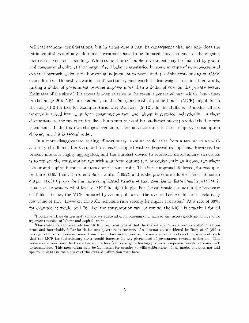
political economy considerations, but in either case it has the consequence that not only does the

initial capital cost of any additional investment have to be �nanced, but also much of the ongoing

increase in recurrent spending. While some share of public investment may be �nanced by grants

and concessional debt, at the margin, �scal balance is satis�ed by some mixture of non-concessional

external borrowing, domestic borrowing, adjustment to taxes, and, possibly, economizing on O&M

expenditures. Domestic taxation is distortionary and exerts a deadweight loss; in other words,

raising a dollar of government revenue imposes more than a dollar of cost on the private sector.

Estimates of the size of this excess burden relative to the revenue generated vary widely, but values

in the range 20%-50% are common, so the 'marginal cost of public funds' (MCF) might be in

the range 1.2-1.5 (see for example Auriol and Warlters, (2012). In the Bu�e et al model, all tax

revenue is raised from a uniform consumption tax, and labour is supplied inelastically. In these

circumstances, the tax operates like a lump sum tax and is non-distortionary provided the tax rate

is constant. If the tax rate changes over time, there is a distortion to inter-temporal consumption

choices, but this is second order.

In a more disaggregated setting, distortionary taxation could arise from a tax structure with

a variety of di�erent tax rates and tax bases, coupled with widespread exemptions. However, the

present model is highly aggregated, and the simplest device to represent distortionary structures

is to replace the consumption tax with a uniform output tax, or equivalently an income tax where

labour and capital incomes are taxed at the same rate. This is the approach followed, for example,

by Barro (1990) and Barro and Sala-i-Matin (1992), and is the procedure adopted here.3 Since an

output tax is a proxy for the more complicated structures that give rise to distortions in practice, it

is natural to wonder what level of MCF it might imply. For the calibration values in the base case

of Table 1 below, the MCF imposed by an output tax at the rate of 17% would be the relatively

low value of 1.13. However, the MCF schedule rises steeply for higher tax rates.4 At a rate of 30%,

for example, it would be 1.76. For the consumption tax, of course, the MCF is exactly 1 for all

3In other work we disaggregate the tax system to allow for consumption taxes to vary across goods and to introduceseparate taxation of labour and capital income.

4One reason for the relatively low MCF in our treatment is that the tax system converts revenue collections from�rms and households dollar-for-dollar into government revenue. An alternative, considered by Berg et al (2014)amongst others, is to assume some 'transmission loss' in the process of remitting tax collections to government, suchthat the MCF for distortionary taxes would increase for any given level of government revenue collection. Thistransmission loss could be treated as a pure loss (an 'iceberg' technology) or as a lump-sum transfer of rents backto households. This mechanism may be important for country-speci�c calibrations of the model but does not addspeci�c insights in the context of the stylized calibration used here.

5

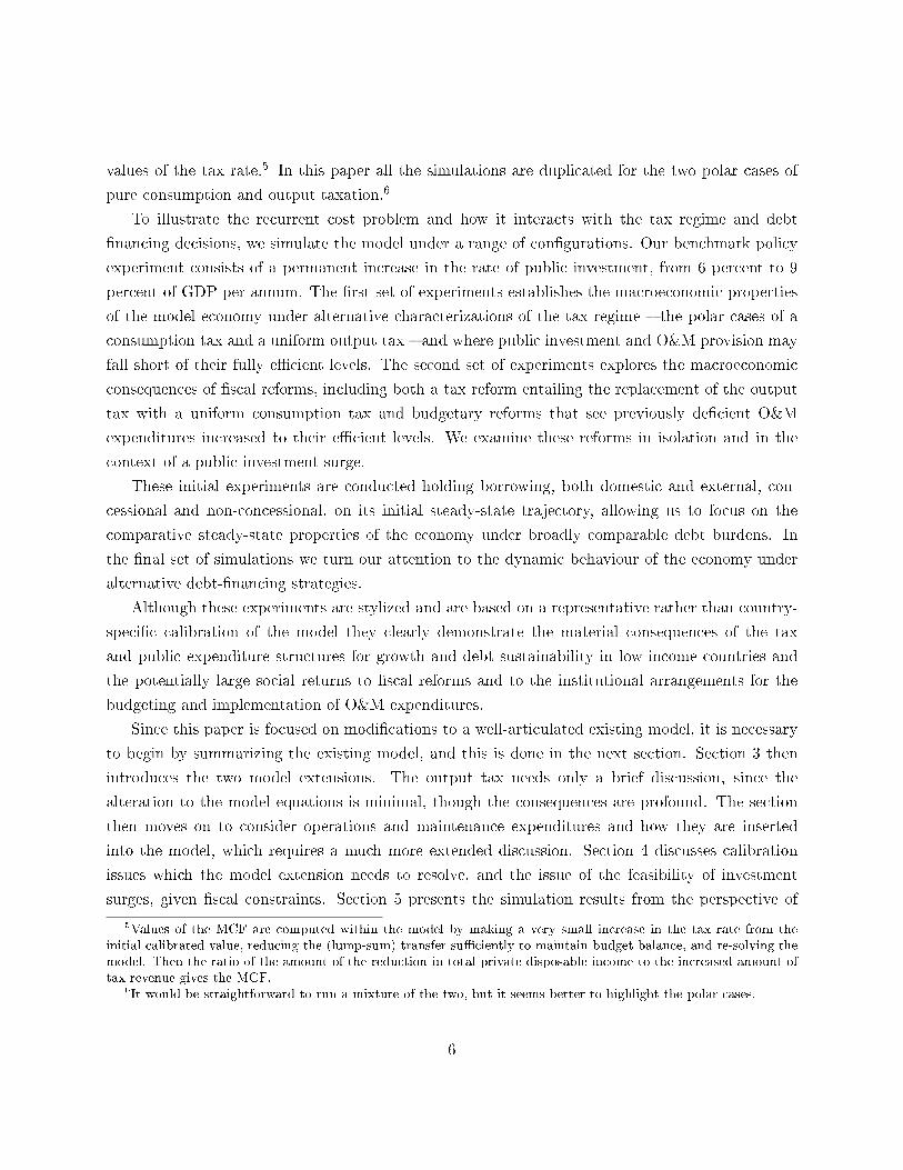
values of the tax rate.5 In this paper all the simulations are duplicated for the two polar cases of

pure consumption and output taxation.6

To illustrate the recurrent cost problem and how it interacts with the tax regime and debt

�nancing decisions, we simulate the model under a range of con�gurations. Our benchmark policy

experiment consists of a permanent increase in the rate of public investment, from 6 percent to 9

percent of GDP per annum. The �rst set of experiments establishes the macroeconomic properties

of the model economy under alternative characterizations of the tax regime � the polar cases of a

consumption tax and a uniform output tax � and where public investment and O&M provision may

fall short of their fully e�cient levels. The second set of experiments explores the macroeconomic

consequences of �scal reforms, including both a tax reform entailing the replacement of the output

tax with a uniform consumption tax and budgetary reforms that see previously de�cient O&M

expenditures increased to their e�cient levels. We examine these reforms in isolation and in the

context of a public investment surge.

These initial experiments are conducted holding borrowing, both domestic and external, con-

cessional and non-concessional, on its initial steady-state trajectory, allowing us to focus on the

comparative steady-state properties of the economy under broadly comparable debt burdens. In

the �nal set of simulations we turn our attention to the dynamic behaviour of the economy under

alternative debt-�nancing strategies.

Although these experiments are stylized and are based on a representative rather than country-

speci�c calibration of the model they clearly demonstrate the material consequences of the tax

and public expenditure structures for growth and debt sustainability in low-income countries and

the potentially large social returns to �scal reforms and to the institutional arrangements for the

budgeting and implementation of O&M expenditures.

Since this paper is focused on modi�cations to a well-articulated existing model, it is necessary

to begin by summarizing the existing model, and this is done in the next section. Section 3 then

introduces the two model extensions. The output tax needs only a brief discussion, since the

alteration to the model equations is minimal, though the consequences are profound. The section

then moves on to consider operations and maintenance expenditures and how they are inserted

into the model, which requires a much more extended discussion. Section 4 discusses calibration

issues which the model extension needs to resolve, and the issue of the feasibility of investment

surges, given �scal constraints. Section 5 presents the simulation results from the perspective of

5Values of the MCF are computed within the model by making a very small increase in the tax rate from theinitial calibrated value, reducing the (lump-sum) transfer su�ciently to maintain budget balance, and re-solving themodel. Then the ratio of the amount of the reduction in total private disposable income to the increased amount oftax revenue gives the MCF.

6It would be straightforward to run a mixture of the two, but it seems better to highlight the polar cases.

6

comparative statics, both for investment surges and the various policy reforms. Section 6 looks at

dynamic perspectives, and section 7 concludes.

2 A stripped-down version of the Bu�e et al model

The framework utilized by Bu�e et al is the standard two-sector model of a small open economy,

where the country produces a traded good qx and a non-traded good qn from private capital k,

labour L, and government-supplied infrastructure z. In addition to these domestically produced

goods, agents can import a traded good for consumption cm and machines mm which can be

combined with the non-traded good to produce factories (private capital) and infrastructure (public

capital). All quantity variables except labour are detrended by (1 + g)t, where g is the exogenous

long-run growth rate of real GDP. The model abstracts from money and all nominal rigidities, but

includes taxation (a uniform consumption tax) and a lump-sum transfer from government to private

agents, as well as grants, remittances and a variety of forms of public and private debt.

Since the present paper extends this model, it is helpful �rst to summarize it. However, it

has a number of features which are neglected here. These include two types of sector-speci�c

externalities in production, adjustment costs incurred in changing the private capital stock, portfolio

adjustment costs associated with foreign liabilities, absorptive capacity constraints associated with

public investment, and also provision for natural resource rents. Shorn of these elaborations, the

stripped-down model is summarized in the rest of this section, starting with the speci�cation of

technology.

2.1 Firms

2.1.1 Technology

In each sector j = n, x, the representative �rm uses a Cobb-Douglas technology to convert labour

Lj,t, private capital kj,t−1, and �e�ectively productive� infrastructure zet−1, which is a public good,

into output:

qx,t = ax(zet−1)ψx(kx,t−1)αx(Lx,t)1−αx (2.1)

qn,t = an(zet−1)ψn(kn,t−1)αn(Ln,t)1−αn (2.2)

where the aj are sector-speci�c productivities.

7

Factories and infrastructure are built by combining imported machines and a non-traded input

(e.g., construction) in �xed proportions, determined by ak and az respectively.7 The supply prices

of private capital and infrastructure are thus:

Pk,t = (1− ak)Pm,t + akPn,t (2.3)

Pz,t = (1− az)Pm,t + azPn,t (2.4)

where Pn is the (relative) price of the non-traded good and Pm is the (relative) price of imported

machinery.

2.1.2 Factor demands

Competitive pro�t-maximizing �rms equate the marginal value product of each input to its factor

price. This yields the input demand equations:

Pn,t(1− αn)qn,tLn,t

= wt (2.5)

Px,t(1− αx)qx,tLx,t

= wt (2.6)

Pn,tαnqn,tkn,t−1

= rn,t (2.7)

Px,tαxqx,tkx,t−1

= rx,t (2.8)

where w is the wage and rj is the rental earned by capital in sector j. Labour is intersectorally

mobile, so the same wage appears in (2.5) and (2.6). Capital is sector-speci�c, and in the presence

of adjustment costs rx may di�er from rn along the transition path. After adjustment is complete

and kx and kn have settled at their equilibrium levels, the rentals are equal. When adjustment costs

are suppressed, as here, the rentals are equal even during the transition.

7The approach in Bu�e et al is slightly di�erent from this, and has the consequence that these supply prices arenot equal to 1 at calibration, as ensured by the present procedure. There are no material consequences of this change.

8

2.2 Consumers

There are two types of private agents, savers and non-savers, with the former and the latter

distinguished by the superscripts s and h respectively. Labour supply of savers is �xed at Ls

while that of non-savers is Lh = aLs with a > 0. The two types of agent consume the domestic

traded good cix,t, the foreign traded good cim,t, and the domestic non-traded good cin,t for i = s, h.

These goods are combined into a CES basket:

cit =

[ρ

1εx (cix,t)

ε−1ε + ρ

1εm(cim,t)

ε−1ε + ρ

1ε

n (cin,t)ε−1ε

] εε−1

(2.9)

for i = s, h where ρx, ρm, and ρn are CES distribution parameters with ρx + ρm + ρn = 1, and

ε is the intra-temporal elasticity of substitution.

The (relative) CPI associated with the basket (2.9) is:

Pt =[ρxP

1−εx,t + ρmP

1−εm,t + ρnP

1−εn,t

] 11−ε

while the demand functions for each good can be expressed as:

cij,t = ρj

(Pj,tPt

)−εcit

for j = x,m, n and i = s, h.

Savers can invest quantities ix and in in private capital that depreciates at the rate δ, pay user

fees charged for infrastructure services according to µze, can buy domestic bonds b - which cannot be

bought in any market by foreigners - and face a real interest rate r.8 They solve the inter-temporal

problem:

Max

∞∑t=0

βt(cst )

1−1/τ

1− 1/τ

subject to:

bst = rx,tksx,t−1 + rn,tk

sn,t−1 + wtL

st +

Rt1 + a

+Tt

1 + a

+1 + rt−1bst−1 − Pk,t

(isx,t + isn,t

)− Ptcst (1 + ht)− µzet−1

(2.10)

(1 + g)ksx,t = isx,t + (1− δ)ksx,t−1 (2.11)

and:

(1 + g)ksn,t = isn,t + (1− δ)ksn,t−1 (2.12)

8The full model also permits them to contract foreign debt, but this feature is suppressed here.

9

where β = 1/[(1 + %)(1 + g)(1−τ)/τ

]is the discount factor; % is the pure time preference rate; τ

is the inter-temporal elasticity of substitution; δ is the depreciation rate; R are remittances; T are

(net) government transfers; h denotes the consumption value added tax (VAT). Remittances and

transfers are proportional to the agent's share in aggregate employment. Observe that the trend

growth rate appears in each of (2.10), (2.11), and (2.12), re�ecting the fact that some variables are

dated at t and others at t− 1.9

The choice variables in the optimization problem are:

cst = cst+1

(β

1 + rt1 + g

PtPt+1

1 + ht1 + ht+1

)−τ(2.13)

rx,t+1

Pk,t+1+ 1− δ = (1 + rt)

Pk,tPk,t+1

(2.14)

rn,t+1

Pk,t+1+ 1− δ = (1 + rt)

Pk,tPk,t+1

(2.15)

Equation (2.13) is an Euler equation in which the slope of the consumption path depends on

the interest rate adjusted for trend growth and on changes in the VAT. The other two equations

are arbitrage conditions, requiring the rate of return on capital in each sector to equal the interest

rate.

Non-savers have the same utility function as that of savers and consume all of their income from

wages, remittances, and transfers each period. The non-saver's budget constraint then reads:

(1 + ht)Ptcht = wtL

h +a

1 + a(Rt + Tt) (2.16)

These hand-to-mouth consumers are a realistic feature of the model and their inclusion breaks

Ricardian equivalence.

Households are aggregated over i = s, h, so that xt = xst + xht for xt = ct, cl,t, Lt, bt, ij,t, kj,t, and

the sub-indices l = x, n,m and j = x, n. Note that bht = ihj,t = khj,t = 0 for j = x, n.

9In Bu�e et al, the domestic bond is indexed to the (relative) price level. However, this is a very ambiguousconcept, and the bonds are treated here as un-indexed.

10

2.3 The Government

2.3.1 Infrastructure, public investment and e�ciency

The model allows for ine�ciencies in public capital creation. Public investment iz produces addi-

tional infrastructure z according to:

(1 + g)zt = (1− δ)zt−1 + iz,t (2.17)

but some of the newly built infrastructure may not be economically valuable, since e�ectively

productive capital zet , which is actually used in technologies (2.1) and (2.2), evolves according to :

zet = sz + s(zt − z) (2.18)

where s, s ∈ [0, 1] are parameters of e�ciency at and o� steady state, and z is public capital at the

(initial) steady state.

Combining equations (2.17) and (2.18) yields:

(1 + g)zet = (1− δ)zet−1 + s(iz,t − iz) + siz (2.19)

where iz = (δ + g)z is public investment at the (initial) steady state. When s < 1, this

speci�cation makes clear that one dollar of additional public investment (iz,t− ¯iz) does not translate

into one dollar of e�ectively productive capital (zet ). Citing empirical estimates, the core simulations

reported in Bu�e et al set s = s = 0.6, and the same assumption is adopted here.

2.3.2 Fiscal adjustment and the public sector budget constraint

The government spends on transfers, debt service, and infrastructure investment. It collects revenue

from the consumption VAT and from user fees for infrastructure services, expressed as a �xed fraction

of recurrent costs, which are restricted to depreciation of e�ective capital at initial prices, that is

µ = fδPz0. When revenues fall short of expenditures, the resulting de�cit is �nanced through

domestic borrowing ∆bt = bt − bt−1, external concessional borrowing ∆dt = dt − dt−1, or external

commercial borrowing ∆dc,t = dc,t − dc,t−1. Hence:

∆bt + ∆dc,t + ∆dt =rt−1 − g

1 + gbt−1 +

rd,t−i − g1 + g

dt−1

+rdc,t−1 − g

1 + gdc,t−1 + Pz,tiz,t + Tt − htPtct −Gt − µzet−1

(2.20)

11

where G denotes grants, and rd and rdc are the real interest rates (in dollars) on concessional

and commercial loans. The interest rate on concessional loans is assumed to be constant rd,t = rd,

while the interest rate on external commercial debt incorporates a risk premium that depends on

the deviations of the external public debt to GDP ratio edt =dt+dc,tyt

from its (initial) steady state

value ed = d+dcy , where yt = Px,tqx,t + Pn.tqn,t is GDP. That is,

rdc,t = rf + υgeηg(edt−ed) (2.21)

where rf is a risk-free world interest rate. If υg > 0 and ηg = 0, this speci�cation provides for

an exogenous risk premium that does not depend on the level of public debt; if both are positive,

the premium is increasing in the external debt to GDP ratio.

Policy makers accept all concessional loans pro�ered by o�cial creditors. The borrowing and

amortization schedule for these loans is �xed exogenously. Given the paths for public investment

and concessional borrowing, the �scal gap before policy adjustment (GAPt)can be de�ned as:

GAPt =1 + rd1 + g

dt−1 − dt +rdc,t−1 − g

1 + gdct−1 +

rt−1 − g1 + g

bt−1

+Pz,tiz,t + T0 − h0Ptct −Gt − µzet−1

(2.22)

GAPt corresponds to expenditures (including interest payments) less revenues and concessional

borrowing, when transfers and taxes are kept at their initial levels T0 and h0 respectively. Using

this de�nition, the government budget constraint (2.20) can be rewritten as:

GAPt = ∆bt + ∆dc,t + (ht − h0)Ptct − (Tt − T0) (2.23)

In other words, given the investment programme, in the short- to medium-term, this gap can

be covered by some mixture of domestic and external commercial borrowing, tax adjustments, and

transfer adjustments.

Debt sustainability requires, however, that the VAT and transfers eventually adjust to cover the

entire gap. Policy makers divide the burden of adjustment between transfer cuts and tax increases,

setting targets as follows:

htargett = h0 + (1− λ)GAPtPtct

(2.24)

T targett = T0 − λGAPt (2.25)

12

where 0 ≤ λ ≤ 1 is a policy parameter that splits the �scal adjustment between taxes and

transfers. Given these targets, reaction functions are de�ned as:

ht = Min {hrt , hu} (2.26)

Tt = Max{T rt , T

l}

(2.27)

where hu is a ceiling for taxes, T l is a �oor for transfers, and hrt and Trt are determined by the

�scal rules:

hrt = ht−1 + λ1(htargett − ht−1) + λ2(xt−1 − xtarget)

yt(2.28)

T rt = Tt−1 + λ3(T targett − Tt−1)− λ4(xt−1 − xtargett ) (2.29)

with λ1, λ2, λ3, λ4 > 0 and x = b or dc, depending on whether the rules respond to domestic or

external commercial debt. The target for debt xtarget is given exogenously.

Given the targets, the reaction functions de�ned in (2.26) - (2.29) together with the budget

constraint (2.23) re�ect the fact that rapid �scal adjustment is painful. Tax increases or expenditure

cuts must be phased in gradually (λ1 > 0, λ3 > 0). On the other hand, policy responds to the debt

overruns that this may induce (λ3 > 0, λ4 > 0).

2.4 Market-clearing conditions and external debt accumulation

Flexible wages and prices ensure that demand continuously equals supply in the labour market:

Lx + Ln = L (2.30)

where the labour supply L = Ls + Lh is �xed.

Aggregating over both types of consumers, and taking into account private and public invest-

ment, the demand for non-tradables is:

qn,t = ρn

(Pn,tPt

)−εct + ak(ix,t + in,t) + aziz,t (2.31)

Finally, consolidating public and private sector budget constraints yields the accounting identity

that growth in the country's net foreign debt equals the di�erence between national spending and

13

national income:

dt − dt−1 + dc,t − dc,t−1 =rd − g1 + g

dt−1 +rdc,t−1 − g

1 + gdc,t−1

+Pz,tiz,t + Pk,t(ix,t + in,t) + Ptct − Pn,tqn,t − Px,tqx,t −Rt −Gt(2.32)

3 Introducing output taxation and operations and maintenance

expenditures

3.1 Output taxation

Private and public budget constraints, and the �scal adjustment rules, need to be adjusted for

the switch in tax instrument, but in very obvious ways. More signi�cant is the impact on factor

demands. Firms still equate the (private) marginal value product of each input to its factor price.

However, the output tax, designated by the rate θ, drives a wedge between the private and social

values:

Pn,t(1− αn)qn,tLn,t

(1− θt) = wt (3.1)

Px,t(1− αx)qx,tLx,t

(1− θt) = wt (3.2)

Pn,tαnqn,tkn,t−1

(1− θt) = rn,t (3.3)

Px,tαxqx,tkx,t−1

(1− θt) = rx,t (3.4)

The real wage is substantially reduced, but consumer purchases from this reduced wage no

longer attract consumption tax. There are no consequences for labour supply, since that is �xed.

The situation is very di�erent for private capital, however. For given steady state r, determined in

the model by savers' preference parameters over the in�nite horizon, and una�ected by the switch

in tax instrument, the output capital ratio must rise by 1/(1 − θ), which requires a sharp fall in

private capital stocks relative to what would have been held under a consumption tax. This implies

a substantial reduction in GDP and in consumption.

14

3.2 Operations and maintenance expenditures

Apart from the use of resources and the need to �nance this, operations and maintenance ex-

penditures a�ect the model in two ways. De�cient maintenance expenditure leads to an increase

in the rate at which the public capital stock depreciates through time while de�cient operations

expenditure reduces the �ow of output produced by the current stock of public capital. Both e�ects

can be temporary: a return to 'full' maintenance and operations expenditures restores the (technical

minimum) depreciation rate and the full �ow of output respectively.10

We distinguish between three di�erent notions of public capital: notional capital (z); installed

capital (zi); and e�ective (or e�ectively productive) capital (ze). The distinction between notional

and installed capital mirrors Bu�e et al, with ine�ciencies in public capital formation meaning that

one unit of notional capital investment generates s ≤ 1 units of installed capital. Hence zi = s.z.11

Installed capital depreciates at a rate determined by the level of maintenance expenditure. The

depreciation rate (of installed capital) is de�ned as

δiz = δz [1 + (1− γm)βδ] (3.5)

where 0 < γm ≤ 1 is the ratio of actual to e�cient maintenance expenditure and βδ ≥ 0

is a measure of excess depreciation. Thus the rate of depreciation is bounded between δz when

maintenance is at its e�cient level and δz(1 + βδ) when maintenance is neglected entirely. The

accelerated loss of installed capital during a period when maintenance is inadequate is permanent;

however, if maintenance expenditure is subsequently improved, following such an episode, the

depreciation rate on the remaining capital falls back to a lower level.

E�ective capital is de�ned as ze = γpzi where 0 < γp ≤ 1 is the ratio of actual to e�cient

operations expenditure.12 For simplicity, these operations and maintenance requirements are treated

as being kinked at the e�cient level; while there is an immediate loss involved when either γ is

allowed to fall below 1, there is no corresponding gain if either is set greater than 1. Such excess

expenditure would just be wasted. Both operations and maintenance expenditures can be modeled

as involving labour inputs, or use of traded and non traded goods, or some combination of the

two. In this note, we focus mainly on the polar case where O&M exclusively involves goods, but

we also illustrate the (fairly considerable) di�erence in behaviour under the alternative polar case

10This is of course a simplifying assumption: in practice, the capital stock may be so degraded as a result ofde�cient maintenance expenditures that it is simply not possible to restore it to 'full' e�ciency without rebuildingafresh.

11Note that zi here corresponds to Bu�e et al 's ze.12It might seem more plausible to model this relation as linear rather than proportional but, for lack of evidence,

it seems best to stick with the simpler formulation.

15

exclusively involving labour inputs. In the goods case, it is assumed that the composition of traded

and non-traded goods is �xed, and is the same as the initial composition of domestic absorption.

Thus, an increase in the level of O&M as a share of total absorption leaves the initial price vectors

undisturbed. The quantities of this composite good are then de�ned respectively as qp,tzit−1and

qm,tzit−1where qj,t = γj,tqj for j = p,m and qj is a measure of 'e�cient' O&M goods expenditures per

unit of installed capital. Similarly, in the polar case of labour inputs, these are de�ned respectively

as lp,tzit−1and lm,tz

it−1where lj,t = γj,tlj for j = p,m and lj is a measure of 'e�cient' O&M labour

inputs per unit of installed capital. These e�cient values could be calibrated on the basis of Heller's

'r-coe�cients', which are estimates of the required annual recurrent expenditure in dollars per dollar

of installed capital.13

We are aware of no quantitative evidence on the scale of the losses in�icted by inadequate O&M,

so the assumptions made here are necessarily speculative. However, we believe that these are quite

conservative. In the simulations reported below, the measure of excess depreciation, β, is set equal

to one. This implies that the depreciation rate would only double, for example from 5% to 10%, even

if maintenance were abandoned entirely. As regards operational expenditures, the proportionality

assumption again seems conservative. These expenditures are composites, and the components are

likely to be required in �xed proportions, or at least to be poor substitutes. Since inadequate

spending is itself ine�cient, it seems most unlikely that the reduction would be allocated optimally

between these components.14

It is necessary to consider how these O&M costs relate to the de�nition of GDP. It might

seem natural to consider operations expenditures, for example, as intermediate goods, necessary

in providing the �nal services of public capital. However, the present model is a pure value-added

model, with no provision for intermediates; and conventional national accounting tends to value

these activities at cost and treat them as part of GDP. Accordingly, that is the practice adopted

here. In the polar goods case, GDP is still de�ned as Y = PxQx + PnQn. The introduction of

positive O&M costs then reduces the amount of Y that is available for private consumption, public

and private investment, and net exports. Where at least part of O&M expenditures are on labour

13See Heller (1991). His estimates are highly dependent on the type of public capital involved, with the coe�cientscovering the huge range between 1% and 72%; the lower values are characteristic of economic infrastructure, the higherones of social infrastructure. Concentrating on maintenance only, for economic infrastructure, Fay and Yepes (2003)estimate values of 2% for electricity generation, rail and road; 3% for water and sanitation; and 8% for mobile andmainline telephones. They stress that these are estimates of the minimum expenditure to ensure the integrity of thesystem, not of the higher levels that would be e�cient. Even so, these magnitudes imply that required expenditureson maintenance of existing capital are typically slightly larger than expenditures on new investment.

14For example, a health clinic may receive inadequate supplies of medicines, even when it is adequately sta�edwith medical personnel. This is likely to reduce services more than proportionally to the reduction in the operationalbudget. It would be straightforward to model this relationship by treating operations as a Leontief relationshipbetween labour inputs and goods expenditures.

16

inputs, the de�nition of GDP becomes Y = PxQx + PnQn + w(lm + lp)zi. When labour inputs to

O&M are positive, this reduces the amount of the given labour force that is available for production

of the two goods.

An important point to note is that it is not assumed that the prior or indeed �nal equilibrium

of the economy is characterized by e�cient O&M. As a consequence of inadequate budget planning

and implementation, exacerbated by the separation of responsibilities for investment decisions and

for O&M, there often is a substantial de�cit in the latter from e�cient levels.15 The problem may

of course be temporarily worsened during an investment surge if that leads to �scal di�culties;

on the other hand, a programme of reforms to public �nancial management may yield a sustained

improvement in the relationship. The present model is designed to permit all these possibilities to

be explored.

Adding in depreciation and debt-�nancing costs the full cost of public investment is given as

[Pom,t(qp,t + qm,t) + (δiz,t + rgt )Pz,t/s

]zit−1 (3.6)

where P om,t = aomPn,t + (1− aom,t)Pm,t is the composite price of operations and maintenance.

This polar case where O&M consists only of goods expenditure is used for illustration.16 The

�rst two terms are the recurrent cash costs of operations and maintenance; the third and fourth

terms correspond to the depreciation and �nancing costs per unit of installed capital, where rgt is

the marginal cost of government (non-concessional) borrowing, recognizing that a unit of installed

capital costs Pz/s to replace. Treating the �nancing cost as equivalent to the cost of borrowing may

seem over-simpli�ed; it appears to imply that �nancing is by means of a perpetuity. However, it is

a more robust approach than that, and this is spelled out in Appendix II.

Finally, we de�ne the user-cost recovery rate as:

µt =[P om,t(fp,tqp,t + fm,tqm,t) + (fd,tδ

iz,t + fr,trt)Pz,t/s

]zit−1 (3.7)

where 0 < fj ≤ 1 for j = p,m, d, r are the recovery rates for each �nancing component.

The reason for distinguishing these rates is that the �nancing components have very di�erent

perceptual properties, and are most unlikely to be treated as an aggregate in budget decisions.

In the calculations reported below, it is assumed that there may be some cost recovery (on an equal

15Rioja (2003) models the issue, and suggests that it would often be e�cient to divert available �nance from newinvestment to increased maintenance of the existing stock. There appears to be less hard numerical evidence inrespect of operations expenditures, but anecdotal evidence as to its common inadequacy abounds.

16The labour case is similar, where the relevant price is the wage; in the mixed case, of course, two prices have tobe tracked.

17

basis) for O&M expenditure, but not for the other two categories of cost. That re�ects the likely

budget operations in many public �nance systems.

4 Calibration issues

The calibration of our model largely mirrors that of Bu�e et al and is summarized in Appendix

I. The introduction of distortionary taxation and the possibility of ine�cient O&M expenditures,

however, requires some modi�cation to the calibration process.

4.1 Distortions in the initial steady states

The original model is set up so that, for any new set of choice parameters (the initial consumption

tax rate, for example), the calibration adjusts various model elasticities and factor inputs to be

consistent with an initial GDP of 100, and for the wage and (most) initial prices to be unity.

While this is convenient for many purposes, it has the disadvantage that the production structure

of the economy varies between experiments: by altering factor inputs, the calibrated productivity

parameters in the production functions (ax and an), and the elasticity of output with respect to

public capital (ψx and ψn) adjust. It is therefore di�cult to compare like with like. In this paper,

since much of the focus is on the impact of various distortions on the outcomes, a di�erent calibration

procedure is required to make it possible to explore the consequences of reforms which reduce these

distortions. The one adopted here is to use the existing procedure to calibrate the 'undistorted' case

where there is a consumption tax and O&M expenditures are at their e�cient levels.17 In that case,

the production parameters are set to yield an initial GDP of 100. These parameters are then locked

down, and calibrations in the various comparable distorted cases (output tax, and/or ine�cient

O&M) are conditional on these structural parameters, which include the production elasticities and

the labour force, but not the capital stocks, which are of course contingent on the distortions. As is

to be expected, initial GDP is less than 100 in the distorted cases, the more so for more pervasive

distortions. Just how far below 100 is a measure of the costs of the distortion.

4.2 E�cient O&M expenditures

Since the model is used to examine the consequences of inadequate operations and maintenance

expenditures, it is important to ensure that the 'e�cient' levels are just that; if the calibration sets

either of the qj or lj too high, a reduction would be budget enhancing. It is necessary that they

17This case is undistorted in a rather restricted sense, since it still has the distortion arising from the ine�cientpublic capital formation process on which the original paper focused.

18

satisfy the condition that the budget does deteriorate when inadequate O&M provision is made. To

keep matters simple, suppose that all steady state comparisons involve the same level of e�ective

public capital, so if O&M is inadequate, higher gross investment is required.

Then for the inadequate maintenance case, it is straightforward to show that the budget dete-

riorates provided:

βδδz(1− fd)Pz/s > (1− fm)Pomqm.

This condition could fail to be satis�ed if fd � fm,which seems highly unlikely, or if βδ is

very small. Note that there is a further welfare loss arising from higher user charges levied on

the private sector. In the absence of cost recovery, or if the two recovery rates are the same, and

public investment is e�cient (s = 1), the condition reduces at calibration in the undistorted case

(Pz = Pom = 1) to:

βδδz > qm (4.1)

For the inadequate operation case, the budget deteriorates provided:

(δz + g)Pz/s > Pomqp

Under the same simplifying assumptions as before, this reduces to:

(δz + g) > qp (4.2)

Cost recovery doesn't enter the story here, because user charges can only be levied on services

provided, and keeping e�ective capital at the same level means no change in user charges. Provided

the two simpler versions of the conditions are satis�ed, they will necessarily also be satis�ed in the

presence of ine�cient investment (s < 1) if Pom/Pz ≤ 1, for the plausible case where fm ≥ fd.18

4.3 Policy rules

Here we follow the design in the original paper, except that with certain exceptions, detailed in the

text, the procedure has been to lock government transfers and aid at their initial level, so that all

�scal adjustments on the path must come from other components which could, in principle, include

temporary or permanent changes in the adequacy of O&M expenditures as well as adjustments to

the level of cost-recovery. The principal experiment we examine is an increase in public investment

which is raised from 6 percent to 9 percent of initial GDP. Throughout most of the paper we assume

18The simulations presented below assume equality of the non-tradable weight in the price of capital goods andoperations and maintenance (az = aom) so that Pom/Pz = 1.

19

that this increase is �nanced through domestic taxation � allowing us to explore the properties of

alternative tax regimes � but we also allow for the investment surge to be debt-�nanced where

the gross (additional) public investment pro�le is matched exactly by non-concessional external

borrowing, but in some �xed proportion. Hence it might be set to cover none, half, or all of the

investment spending at each date in the surge, with the balance �nanced by some combination of

tax and domestic debt. Concessional external debt is held constant throughout.

5 Simulation results: comparative statics

5.1 Public investment, de�cient O&M and alternative tax regimes

Tables 1 to 3 describe the key features of the model in the context of a public investment surge.

Here we con�ne our attention to the steady state properties of the model and limit our attention

to programmes in which public investment is �nanced exclusively from domestic taxation; in the

dynamic runs examined later we provide for external and domestic bond �nancing.19 In all cases,

the comparison is between an initial steady state where public investment is stationary at 6% of

GDP, and one where it has been raised by 50% of that level, i.e. by 3% of initial GDP, but to a level

below 9% of �nal GDP, given the induced growth in the latter. Features that are common to all the

tables are the private cost of capital, at 10% per annum; and the steady state ine�ciency in public

capital creation (s = 0.6 throughout). Public and private capital depreciate at 5% per annum,

though the depreciation of the public infrastructure capital will rise if maintenance expenditure is

inadequate. The social return to public infrastructure capital in the undistorted initial steady state

is set to 25% and the initial social return to public investment is 13%. The derivation of these

calibration parameters is described in Appendix III.

Table 1, which describes base cases and is analogous to the base case in the original paper

(Bu�e et al., 2012, Table 3), compares outcomes under a set of runs for the consumption tax and

a corresponding set for the output tax. The latter is set at an initial rate of 17 per cent, to re�ect

a typical ratio of tax revenue to GDP in low-income countries. Given the parametrization of the

original model, a consumption tax at a rate of 20 per cent generates broadly similar revenue. Any

di�erence in initial revenue yield is taken up by a compensating variation in the lump-sum transfer

19An alternative strategy would entail maintaining taxes and borrowing �xed at their initial values and �nancingthe increased public investment by reducing other component of public expenditure. The model used here is, however,not well suited to examining this case. Other than O&M expenditures, no government services are produced so that allnon-O&M recurrent expenditures consist of lump-sum non-distortionary transfers to households. In macroeconomicterms, therefore, an expenditure-switching strategy that sees transfers reduced is equivalent, across steady states, toone in which the investment surge is �nanced by increasing the uniform consumption tax. The alternative of �nancingpublic investment by scaling back O&M expenditures will have features similar to an extreme version of the case weanalyse in Table 3 below.

20

from government to households.20 The �nancing of the investment surge is entirely via changes in

the relevant tax rate, with the transfer held �xed and no change in borrowing, either domestic or

external. E�cient operations expenditures and e�cient maintenance expenditures are both equal

to 2.5 cents per dollar of installed public capital, so that O&M outgoings are 5 cents per dollar. For

the present, it is assumed that no cost recovery takes place.

Column (1) describes the e�ect of the investment surge in the 'undistorted' case. Public

investment crowds-in private investment, which rises by $1.78 for each $1 of public investment.

GDP increases by 14.6% between steady states in a broadly balanced fashion; the real exchange

rate appreciates by just over 2% between steady states. Real product wages increase by 15%;

combined with the higher level of public capital, this causes the budgetary cost of O&M to rise to

3.6% of (current) GDP which, in turn, requires an increase in the consumption tax rate of just over

3%. Thus far � excepting the O&M expenditure � the results exactly mirror Bu�e et al.

Introducing O&M ine�ciencies has a marked e�ect on the initial steady state level of GDP.

Relative to the e�cient level of 100%, γm = 0.8 lowers initial GDP by more than 7 percentage

points, γp = 0.8 lowers it by more than 10 points, and γm = γp = 0.8 by more than 17 points

[columns (2) to (4)]. Conditional on these di�erences in the initial level of GDP, however, the

response to the investment surge is broadly similar, with output and consumption growing by more

or less the same amount.

Also interesting is the comparison between the consumption tax and output tax. Consider �rst

the comparison between columns (1) and (5). Here, even with e�cient O&M expenditures, initial

GDP is more than 19 percent lower when the economy operates under an output tax regime , the

damage being caused by the sharp reduction in equilibrium private capital induced by the tax.

Moreover, between steady states the distortionary tax reduces the growth in GDP and consumption

in response to the investment surge, again due to the lower rate of private capital accumulation

(the crowding-in of private capital is only 60 percent of that achieved under the consumption tax).

And while in both the consumption and output tax cases, real GDP rises very slightly further in

the �nal steady state as O&M distortions become more severe � by 14.61% in column 4, as opposed

to 14.59% in column 1 in the case of the consumption tax and by 12.97% in column 8 as opposed

to 12.54% in column 5 in the output tax case � these higher growth rates are from lower initial

starting points (at which the initial return to public investment is correspondingly higher).

20In principle, the transfer could be held constant between tax regimes in order to calibrate the initial consumptiontax. Given the non-distortionary properties of the consumption tax in the steady state, the model's behaviour isinvariant to this choice.

21

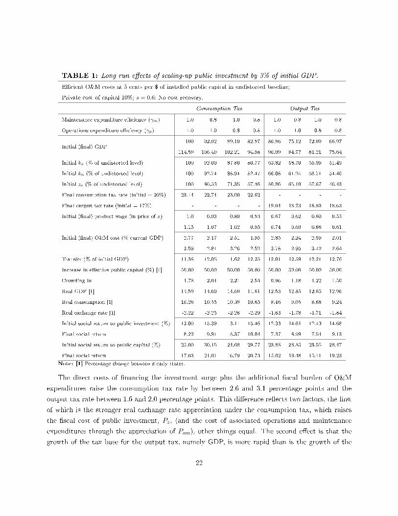
TABLE 1: Long run e�ects of scaling-up public investment by 3% of initial GDP.

E�cient O&M costs at 5 cents per $ of installed public capital in undistorted baseline;

Private cost of capital 10%; s = 0.6; No cost recovery.

Consumption Tax Output Tax

Maintenance expenditure e�ciency (γm) 1.0 0.8 1.0 0.8 1.0 0.8 1.0 0.8

Operations expenditure e�ciency (γp) 1.0 1.0 0.8 0.8 1.0 1.0 0.8 0.8

Initial (�nal) GDP100 92.92 89.19 82.87 80.86 75.12 72.09 66.97

114.59 106.49 102.21 94.98 90.99 84.77 81.21 75.64

Initial kx (% of undistorted level) 100 92.00 87.80 80.77 63.82 58.70 55.99 51.49

Initial kn (% of undistorted level) 100 92.74 88.94 82.47 66.08 61.24 58.71 54.40

Initial ze (% of undistorted level) 100 80.53 71.35 57.46 80.86 65.10 57.67 46.43

Final consumption tax rate (initial = 20%) 23.14 22.74 23.00 22.62 - - - -

Final output tax rate (initial = 17%) - - - - 19.04 18.73 18.93 18.63

Initial (�nal) product wage (in price of x) 1.0 0.93 0.89 0.83 0.67 0.62 0.60 0.55

1.15 1.07 1.02 0.95 0.74 0.69 0.66 0.61

Initial (�nal) O&M cost (% current GDP) 2.77 2.17 2.51 1.95 2.85 2.24 2.59 2.01

3.59 2.81 3.26 2.52 3.78 2.95 3.42 2.64

Transfer (% of initial GDP) 11.38 12.05 11.62 12.25 12.01 12.59 12.21 12.76

Increase in e�ective public capital (%) [1] 50.00 50.00 50.00 50.00 50.00 50.00 50.00 50.00

Crowding In 1.78 2.04 2.21 2.53 0.96 1.18 1.22 1.50

Real GDP [1] 14.59 14.60 14.60 14.61 12.53 12.85 12.65 12.96

Real consumption [1] 10.26 10.55 10.38 10.65 8.46 9.05 8.68 9.24

Real exchange rate [1] -2.22 -2.25 -2.26 -2.29 -1.63 -1.78 -1.71 -1.84

Initial social return to public investment (%) 13.00 15.39 13.11 15.46 12.33 14.61 12.43 14.68

Final social return 8.22 9.91 8.37 10.04 7.37 8.99 7.54 9.13

Initial social return to public capital (%) 25.00 30.15 24.68 29.77 23.88 28.85 23.55 28.47

Final social return 17.03 21.01 16.79 20.73 15.62 19.48 15.41 19.23

Note: [1] Percentage change between steady states.

The direct costs of �nancing the investment surge plus the additional �scal burden of O&M

expenditures raise the consumption tax rate by between 2.6 and 3.1 percentage points and the

output tax rate between 1.6 and 2.0 percentage points. This di�erence re�ects two factors, the �rst

of which is the stronger real exchange rate appreciation under the consumption tax, which raises

the �scal cost of public investment, Pz, (and the cost of associated operations and maintenance

expenditures through the appreciation of Pom), other things equal. The second e�ect is that the

growth of the tax base for the output tax, namely GDP, is more rapid than is the growth of the

22

base for the consumption tax, namely consumption itself. The required increase in the output tax

rate is therefore less than that for the consumption tax.

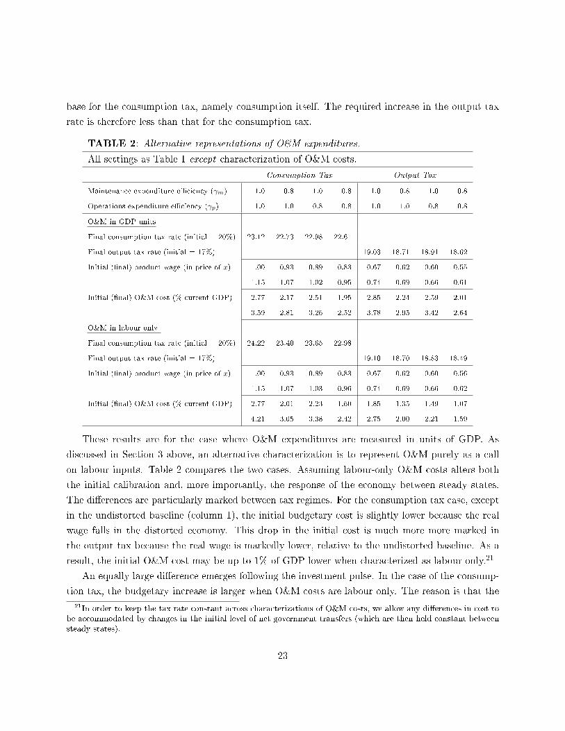
TABLE 2: Alternative representations of O&M expenditures.

All settings as Table 1 except characterization of O&M costs.


Maintenance expenditure e�ciency (γm) 1.0 0.8 1.0 0.8 1.0 0.8 1.0 0.8

Operations expenditure e�ciency (γp) 1.0 1.0 0.8 0.8 1.0 1.0 0.8 0.8

O&M in GDP units




1.15 1.07 1.02 0.95 0.74 0.69 0.66 0.61


3.59 2.81 3.26 2.52 3.78 2.95 3.42 2.64

O&M in labour only




1.15 1.07 1.03 0.96 0.74 0.69 0.66 0.62


4.21 3.05 3.38 2.42 2.75 2.00 2.21 1.59

These results are for the case where O&M expenditures are measured in units of GDP. As

discussed in Section 3 above, an alternative characterization is to represent O&M purely as a call

on labour inputs. Table 2 compares the two cases. Assuming labour-only O&M costs alters both

the initial calibration and, more importantly, the response of the economy between steady states.

The di�erences are particularly marked between tax regimes. For the consumption tax case, except

in the undistorted baseline (column 1), the initial budgetary cost is slightly lower because the real

wage falls in the distorted economy. This drop in the initial cost is much more more marked in

the output tax because the real wage is markedly lower, relative to the undistorted baseline. As a

result, the initial O&M cost may be up to 1% of GDP lower when characterized as labour only.21

An equally large di�erence emerges following the investment pulse. In the case of the consump-

tion tax, the budgetary increase is larger when O&M costs are labour only. The reason is that the

21In order to keep the tax rate constant across characterizations of O&M costs, we allow any di�erences in cost tobe accommodated by changes in the initial level of net government transfers (which are then held constant betweensteady states).

23

public investment surge and associated crowding in of private capital drives up the product wage

and hence the O&M wage bill. By contrast, the rise in the output tax rate in columns 5-8 is much

the same in the two cases, and on average the increase is somewhat lower. This is because two

opposing e�ects are more or less neutralizing each other. One is the rise in the wage following the

the investment surge, as before. The other is the fact that the output tax drives the initial product

wage down, so that the rise is from a much reduced base. Indeed, the initial product wage is reduced

sharply (by a third). This is partially because the product wage is reduced directly by the tax, and

partially because it is reduced indirectly by the fall in the private capital stock, lowering the pre-tax

marginal product of labour. These e�ects are exacerbated by O&M ine�ciency. The reduction in

the public sector wage bill is most marked in the most distorted cases, which is why the increase in

required tax revenue is reduced for these.22

Finally in this section we examine the long-run e�ects of a public investment surge that is not

matched by a commensurate increase in O&M expenditures. To avoid repetition, we take as our

baseline the output tax case where O&M expenditures are initially at 80% of their e�cient levels

(γm = γp = 0.8) which corresponds to column (8) of Table 1. Public investment is increased

by 3% of initial GDP as before but the provision against the additional installed public capital

is insu�cient to maintain overall O&M at its baseline rate when spread across the new higher

installed capital. Speci�cally, we calibrate this short-fall such that when one or both of O&M are

de�cient, the 'marginal γ' is only half its infra-marginal rate. The e�ective or average values of γs

are the weighted average of 0.8 and 0.4, with the weight re�ecting the relative size of the addition

to the installed capital stock: given the scale of the investment surge this bring the relevant γs to

0.67 in the de�cient cases. Under our calibration the budgetary costs of cutting either operations

or maintenance expenditures are equivalent ex ante. When neither O&M rise proportionally with

public investment, growth in output falls sharply, from 13.0% to only 1.9% between steady states.

As columns (2) and (3) of the table indicate, de�cient operations expenditure account for the greater

share of the damage; here the e�ective public capital stock grows by only 25% between steady states

compared to the baseline of 50%, whereas when maintenance is de�cient (at the same ex ante �scal

cost) the e�ective capital stock grows by 37.8%.23 In all cases, however, paring back O&M is a

false economy with the steady-state tax rate between 0.2 and 1.5 percentage points above that

required when baseline O&M levels are maintained. In the extreme (not reported in the table),

22The patterns of the results presented here are broadly invariant to assumptions about the initial social rate ofreturn to public capital and the associated social return to public investment, elevated or depressed according tothese assumptions of higher and lower productivity respectively. These results are available on request.

23This di�erence re�ects, of course, the parameterization chosen in our calibration: if de�cient maintenanceexpenditures were punished by a sharper increase in the depreciation rate in 3.5, for example, the gap betweenthe two cases would diminish.

24

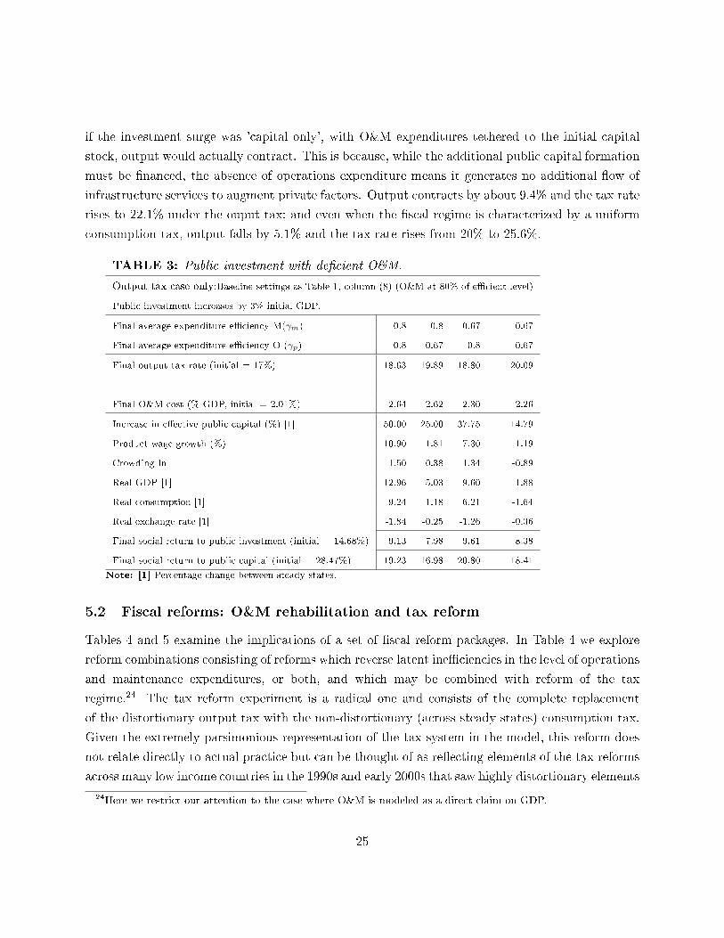
if the investment surge was 'capital only', with O&M expenditures tethered to the initial capital

stock, output would actually contract. This is because, while the additional public capital formation

must be �nanced, the absence of operations expenditure means it generates no additional �ow of

infrastructure services to augment private factors. Output contracts by about 9.4% and the tax rate

rises to 22.1% under the ouput tax; and even when the �scal regime is characterized by a uniform

consumption tax, output falls by 5.1% and the tax rate rises from 20% to 25.6%.

TABLE 3: Public investment with de�cient O&M.

Output tax case only;Baseline settings as Table 1, column (8) (O&M at 80% of e�cient level)

Public investment increases by 3% initial GDP.

Final average expenditure e�ciency M(γm) 0.8 0.8 0.67 0.67

Final average expenditure e�ciency O (γp) 0.8 0.67 0.8 0.67

Final output tax rate (initial = 17%) 18.63 19.89 18.80 20.09

Final O&M cost (% GDP, initial = 2.01%) 2.64 2.62 2.30 2.26

Increase in e�ective public capital (%) [1] 50.00 25.00 37.75 14.79

Product wage growth (%) 10.90 1.81 7.30 -1.19

Crowding In 1.50 0.38 1.34 -0.89

Real GDP [1] 12.96 5.03 9.60 1.88

Real consumption [1] 9.24 1.18 6.21 -1.64

Real exchange rate [1] -1.84 -0.25 -1.26 -0.36

Final social return to public investment (initial = 14.68%) 9.13 7.98 9.61 8.38

Final social return to public capital (initial = 28.47%) 19.23 16.98 20.80 18.41


5.2 Fiscal reforms: O&M rehabilitation and tax reform

Tables 4 and 5 examine the implications of a set of �scal reform packages. In Table 4 we explore

reform combinations consisting of reforms which reverse latent ine�ciencies in the level of operations

and maintenance expenditures, or both, and which may be combined with reform of the tax

regime.24 The tax reform experiment is a radical one and consists of the complete replacement

of the distortionary output tax with the non-distortionary (across steady states) consumption tax.

Given the extremely parsimonious representation of the tax system in the model, this reform does

not relate directly to actual practice but can be thought of as re�ecting elements of the tax reforms

across many low income countries in the 1990s and early 2000s that saw highly distortionary elements

24Here we restrict our attention to the case where O&M is modeled as a direct claim on GDP.

25

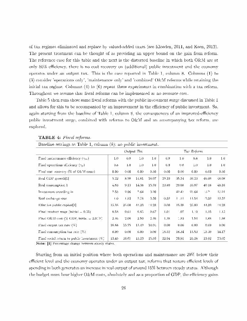
of tax regimes eliminated and replace by valued-added taxes (see Kloeden, 2011, and Keen, 2012).

The present treatment can be thought of as providing an upper bound on the gain from reform.

The reference case for this table and the next is the distorted baseline in which both O&M are at

only 80% e�ciency, there is no cost recovery on (additional) public investment and the economy

operates under an output tax. This is the case reported in Table 1, column 8. Columns (1) to

(3) consider 'operations-only', 'maintenance-only' and 'combined' O&M reforms while retaining the

initial tax regime. Columns (4) to (6) repeat these experiments in combination with a tax reform.

Throughout we assume that �scal reforms can be implemented at no resource cost.

Table 5 then runs these same �scal reforms with the public investment surge discussed in Table 1

and allows for this to be accompanied by an improvement in the e�ciency of public investment. So,

again starting from the baseline of Table 1, column 8, the consequences of an improved-e�ciency

public investment surge, combined with reforms to O&M and an accompanying tax reform, are

explored.

TABLE 4: Fiscal reforms.

Baseline settings as Table 1, column (8); no public investment.

Output Tax Tax Reform

Final maintenance e�ciency (γm) 1.0 0.8 1.0 1.0 0.8 1.0 0.8 1.0 1.0

Final operations e�ciency (γp) 0.8 1.0 1.0 1.0 0.8 0.8 1.0 1.0 1.0

Final cost recovery (% of O&M costs) 0.00 0.00 0.00 0.50 0.00 0.00 0.00 0.00 0.50

Real GDP growth[1] 5.22 8.98 14.61 16.07 29.19 35.54 39.23 46.08 46.08

Real consumption[1] 4.83 9.13 14.38 15.70 23.89 29.68 33.87 40.16 40.16

Investment crowding-in 2.55 2.96 2.64 3.20 - 42.47 27.64 17.21 17.21

Real exchange rate -1.0 -1.83 -2.78 -3.30 -10.32 -11.11 -11.54 -12.32 -12.32

E�ective public capital[1] 15.38 25.00 44.23 44.23 0.00 15.38 25.00 44.23 44.23

Final product wage (initial = 0.55) 0.58 0.61 0.65 0.67 1.01 1.07 1.10 1.15 1.15

Final O&M cost (% GDP, initial = 2.01%) 2.46 2.06 2.50 2.46 1.48 1.83 1.54 1.88 1.88

Final output tax rate (%) 16.68 15.75 15.49 14.04 0.00 0.00 0.00 0.00 0.00

Final consumption tax rate (%) 0.00 0.00 0.00 0.00 16.52 16.34 15.53 15.39 14.17

Final social return to public investment (%) 13.45 16.67 15.23 15.59 22.94 20.91 25.28 23.02 23.02


Starting from an initial position where both operations and maintenance are 20% below their

e�cient level and the economy operates under an output tax, reforms that restore e�cient levels of

spending in both generates an increase in real output of around 15% between steady states. Although

the budget must bear higher O&M costs, absolutely and as a proportion of GDP, the e�ciency gains

26

accruing to the enhanced stock of e�ective public capital crowds-in private investment and allows

these higher budgetary costs to be �nanced at a lower rate of output tax (recall that in Table 4

there is no increase in the net public investment rate, so that the measured increase in e�ective

public capital entirely re�ects e�ciency gains: bringing both O&M to their e�cient levels raises

the e�ective public capital stock by 44%). The e�ects are more or less additive between improving

operations and improving maintenance expenditures, although the returns to improving operations

e�ciency has a larger marginal impact on economic performance. Clearly the mechanisms di�er,

with improved e�ciency of operations enhancing the productivity of the entire capital stock and

improved e�ciency of maintenance altering the depreciation rate henceforth for any given level of

e�ciency. That the operations e�ect dominates here is simply a re�ection of the uncertainties of

our calibration: our estimates of the rate at which de�cient maintenance expenditure accelerates

the depreciation of public capital and of the elasticity of the e�ectiveness of the installed capital

stock to operations expenditures are highly speculative.

When accompanied by a wholesale tax reform, the output and welfare gains are even more

substantial. Aggregate consumption rises by almost 24% across steady states as a result of a de�cit

neutral tax reform, and by 40% if this is accompanied by reforms to O&M spending that operate

on the intensive margin of public capital. The mechanism for output growth is the very substantial

increase in private investment across steady states induced by the removal of tax on output: in

the case where tax reform is accompanied by O&M reforms, for example, the capital stock in the

exportable sector rises by 132% between steady steady states and that in the non-tradable sector

by 106%. The surge in absorption drives up real product wages, measured in terms of the tradable

good, very sharply (from 0.55 to 1.15 in the comprehensive reform case shown in column 8) although

the e�ect on real consumption wages will be somewhat dampened by the sharp appreciation of the

real exchange rate, which in this instance is approximately 12% above its initial steady-state value.

27

TABLE 5: Fiscal reforms with public investment.

Baseline settings as Table 1, column (8); public investment increased by 3% of GDP

Output Tax Tax Reform

Final maintenance e�ciency (γm) 0.8 0.8 1.0 1.0 0.8 0.8 1.0 1.0

Final operations e�ciency (γp) 0.8 0.8 1.0 1.0 0.8 0.8 1.0 1.0

E�ciency of public investment 0.6 1.0 1.0 1.0 0.6 1.0 1.0 1.0

Cost recovery (on new investment) 0.00 0.00 0.00 0.50 0.00 0.00 0.00 0.50

Real GDP growth[1] 12.97 21.83 41.67 43.45 48.07 58.39 81.98 81.98

Real consumption growth [1] 9.25 17.90 37.00 38.63 38.35 48.21 70.51 70.51

Investment crowding-in 1.50 1.75 1.70 1.87 15.65 10.67 6.40 6.40

Real exchange rate -1.85 -3.39 �6.29 -6.79 -12.53 -13.61 -15.79 -15.79

E�ective public capital[1] 50.00 83.33 177.24 177.24 50.00 83.33 177.24 177.24

Final product wage (initial = 0.55) 0.61 0.67 0.80 0.82 1.16 1.25 1.44 1.44

Final O&M cost (% GDP, initial = 2.01%) 2.64 2.98 3.82 3.77 1.92 2.19 2.85 2.85

Final output tax rate (%) 18.62 17.72 16.40 14.98 0.00 0.00 0.00 0.00

Final consumption tax rate (%) 0.00 0.00 0.00 0.00 18.38 17.71 16.74 14.81


The �scal consequences of reform are highly attractive. The restoration of e�cient O&M allows

for a modest decline in the steady-state output tax rates, from 17% to 15.49%, and by a further 1.5%

if user fees cover half of the O&M costs associated with public capital formation and operation.

In the case of a tax reform, the growth e�ects are su�ciently powerful to ensure both that the

O&M cost share in GDP falls and that the consumption tax rate required to balance the budget

settles at around 15.4%. In other words the economy can achieve a lower rate of tax on a narrower

tax base. In this case too, of course, a measure of cost recovery lowers the consumption tax rate

although in contrast to the output tax rate, the substitution of (lump-sum) cost recovery for the

non-distortionary consumption tax does not otherwise alter the equilibrium outcome.

The powerfully welfare-enhancing e�ects of �scal reform are reinforced when combined with

a public investment surge, as shown in Table 5. As Bu�e et al show in the context of a non-

distortionary tax, improvements in the e�ciency of public investment - so that the quantity of

installed public capital realized per unit of investment is increased � can sharply increase growth,

by a factor of almost three, and drive down the required tax rate.25 A similar but more muted e�ect

occurs in a distortionary tax regime considered here � output less than doubles between columns

1 and 2 of Table 5 while the required output tax rate increases. But when investment e�ciencies

25Bu�e et al., 2012, Table 3

28

are harnessed with broader �scal reforms the crowding-in e�ect is su�ciently strong that the public

investment surge can be �nanced with lower output tax rates and by much lower consumption tax

rates in the case of an investment-cum-tax-reform programme.

6 Debt �nancing

The analysis in the previous section assumes the public investment surge is entirely tax-�nanced.

The next step is to examine how external and/or domestic debt �nancing may substitute for tax

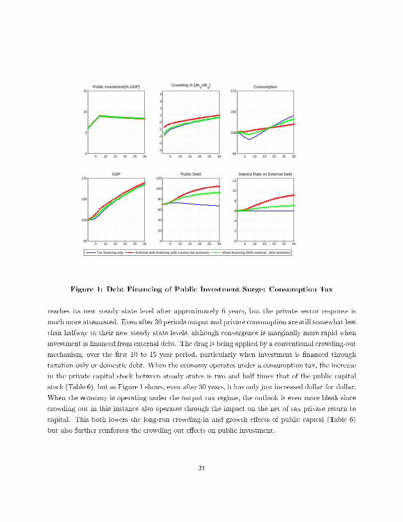
�nancing. Table 6 reports the comparative steady-state outcomes under three �nancing arrange-

ments, separately for the two tax regimes, while Figures 1 and 2 illustrate elements of the dynamic

adjustment between the steady states. The �rst three columns of Table 6 (and Figure 1) describe the

economy operating under a consumption tax and the second three (and Figure 2) the outcome for the

output tax. In each case the �rst column corresponds to the tax-only results from Table 1, in which

domestic debt is held at a constant share of (initial) GDP. In the second column, the investment

costs are fully �nanced by non-concessional borrowing, and in the �nal column the investment costs

are borne equally between domestic and external debt.26 The supply curve for non-concessional

debt is upward sloping with the interest rate rising by approximately 0.9 percentage points for each

10% of GDP increase in debt.

The key point from this table follows directly from the government's inter-temporal budget

constraint: the rise in the public debt burden between steady-states necessarily entails a higher tax

rate, ceteris paribus. Debt �nancing adds between 3.4 and 4.1 percentage points to the required

consumption tax rate and between 3.3 and 3.6 percentage points to the output tax rate. While

the additional tax burden necessarily eats directly into private consumption between steady states,

the impact on output growth (and the social return to public investment) when revenue is raised

through a consumption tax is minimal.

26This is true ex ante, although not ex post because of the evolution of prices in general equilibrium between steadystates.

29

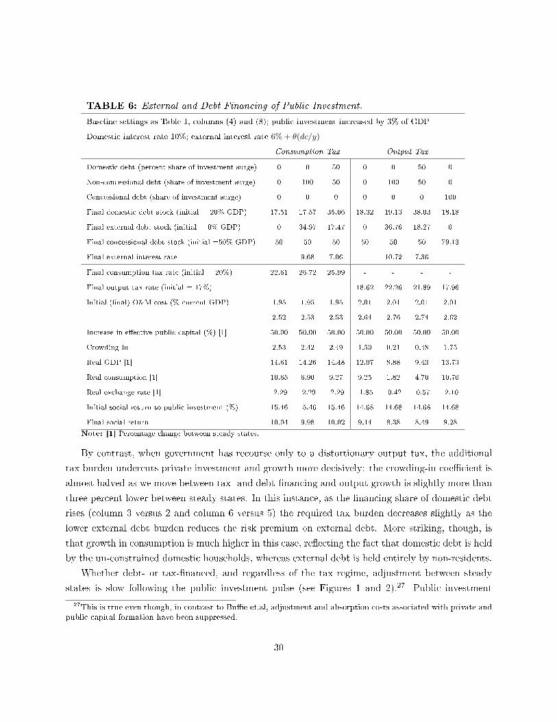
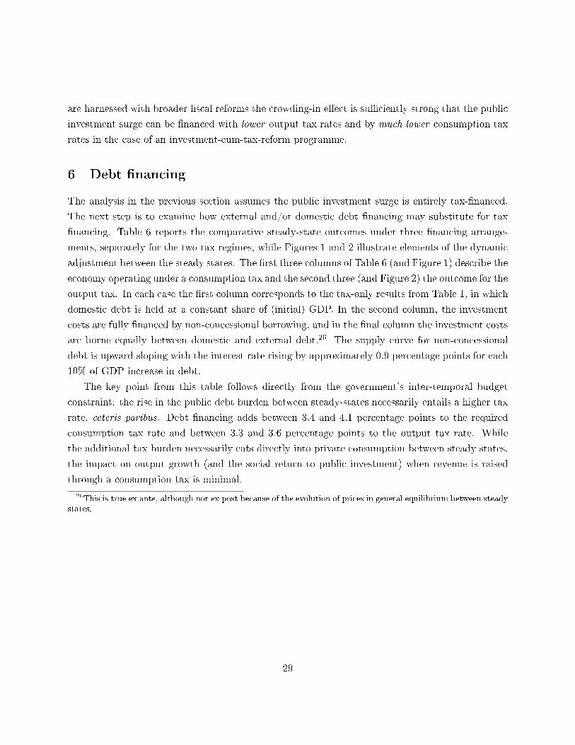
TABLE 6: External and Debt Financing of Public Investment.

Baseline settings as Table 1, columns (4) and (8); public investment increased by 3% of GDP

Domestic interest rate 10%; external interest rate 6% + θ(dc/y)


Domestic debt (percent share of investment surge) 0 0 50 0 0 50 0

Non-concessional debt (share of investment surge) 0 100 50 0 100 50 0

Concessional debt (share of investment surge) 0 0 0 0 0 0 100

Final domestic debt stock (initial = 20% GDP) 17.51 17.57 35.06 18.32 19.13 38.03 18.18

Final external debt stock (initial = 0% GDP) 0 34.97 17.47 0 36.76 18.27 0

Final concessional debt stock (initial =50% GDP) 50 50 50 50 50 50 79.13

Final external interest rate - 9.68 7.06 - 10.72 7.36 -

Final consumption tax rate (initial = 20%) 22.61 26.72 25.99 - - - -

Final output tax rate (initial = 17%) - - - 18.62 22.26 21.89 17.96

Initial (�nal) O&M cost (% current GDP) 1.95 1.95 1.95 2.01 2.01 2.01 2.01

2.52 2.53 2.53 2.64 2.76 2.74 2.62

Increase in e�ective public capital (%) [1] 50.00 50.00 50.00 50.00 50.00 50.00 50.00

Crowding In 2.53 2.42 2.49 1.50 0.21 0.48 1.75

Real GDP [1] 14.61 14.26 14.48 12.97 8.88 9.43 13.73

Real consumption [1] 10.65 6.90 9.27 9.25 1.82 4.70 10.70

Real exchange rate [1] -2.29 -2.29 -2.29 -1.85 -0.42 -0.57 -2.10

Initial social return to public investment (%) 15.46 15.46 15.46 14.68 14.68 14.68 14.68

Final social return 10.04 9.98 10.02 9.14 8.38 8.49 9.28


By contrast, when government has recourse only to a distortionary output tax, the additional

tax burden undercuts private investment and growth more decisively: the crowding-in coe�cient is

almost halved as we move between tax- and debt-�nancing and output growth is slightly more than

three percent lower between steady states. In this instance, as the �nancing share of domestic debt

rises (column 3 versus 2 and column 6 versus 5) the required tax burden decreases slightly as the

lower external debt burden reduces the risk premium on external debt. More striking, though, is

that growth in consumption is much higher in this case, re�ecting the fact that domestic debt is held

by the un-constrained domestic households, whereas external debt is held entirely by non-residents.

Whether debt- or tax-�nanced, and regardless of the tax regime, adjustment between steady

states is slow following the public investment pulse (see Figures 1 and 2).27 Public investment

27This is true even though, in contrast to Bu�e et.al, adjustment and absorption costs associated with private andpublic capital formation have been suppressed.

30

5 10 15 20 25 300

5

10

15Public Investment(% GDP)

5 10 15 20 25 30

-4

-3

-2

-1

0

1

2

3

4

Crowding-In [dKp/dK

g]

5 10 15 20 25 3095

100

105

110Consumption

5 10 15 20 25 3095

100

105

110GDP

5 10 15 20 25 300

20

40

60

80

100

120Public Debt

5 10 15 20 25 300

2

4

6

8

10

12

Interest Rate on External Debt

Tax financing only External debt financing (with country risk premium) Mixed financing (50% external , 50% domestic)

Figure 1: Debt Financing of Public Investment Surge: Consumption Tax

reaches its new steady state level after approximately 6 years, but the private sector response is

much more attenuated. Even after 30 periods output and private consumption are still somewhat less

than halfway to their new steady state levels, although convergence is marginally more rapid when

investment is �nanced from external debt. The drag is being applied by a conventional crowding-out

mechanism, over the �rst 10 to 15 year period, particularly when investment is �nanced through

taxation only or domestic debt. When the economy operates under a consumption tax, the increase

in the private capital stock between steady states is two and half times that of the public capital

stock (Table 6), but as Figure 1 shows, even after 30 years, it has only just increased dollar-for-dollar.

When the economy is operating under the output tax regime, the outlook is even more bleak since

crowding out in this instance also operates through the impact on the net of tax private return to

capital. This both lowers the long-run crowding-in and growth e�ects of public capital (Table 6)

but also further reinforces the crowding out e�ects on public investment.

31

5 10 15 20 25 300

5

10

15Public Investment (% GDP)

5 10 15 20 25 30

-4

-3

-2

-1

0

1

2

3

4

Crowding-In [dKp/dK

g]

5 10 15 20 25 3095

100

105

110Consumption

5 10 15 20 25 3095

100

105

110GDP

5 10 15 20 25 300

20

40

60

80

100

120Public Debt

5 10 15 20 25 300

2

4

6

8

10

12

Interest Rate on External Debt

Tax financing only External debt financing (with country risk premium) Mixed financing (50% external , 50% domestic)

Figure 2: Debt Financing of Public Investment Surge: Output Tax

6.1 Constraints on taxation, debt and the tax pro�le

The rationale for wanting to investigate the whole issue of debt sustainability presupposes that

circumstances may arise in which debt is not sustainable, and some form of forgiveness or default

must ensue. Alternatively, the government or its creditors might come to the conclusion that

a programme would in due course lead to unsustainability if it were persevered with, and that a

change in the programme was necessary in order to avoid this. Modeling the former case, debt would

eventually begin to explode, and the model would crash. In the latter, a switch to a less ambitious

programme would be put in place before that happened. These types of exercise would permit

exploration of how infeasible policies might arise, the path of the economy up to the crash, and

the options for successful recti�cation. It would also be possible to explore changes in circumstance

which would turn a feasible programme into an infeasible one.

Unfortunately, the type of model used here is not well designed to explore such possibilities; after

any initial shock, the model's solution procedure relies on perfect foresight by the saving households.

32

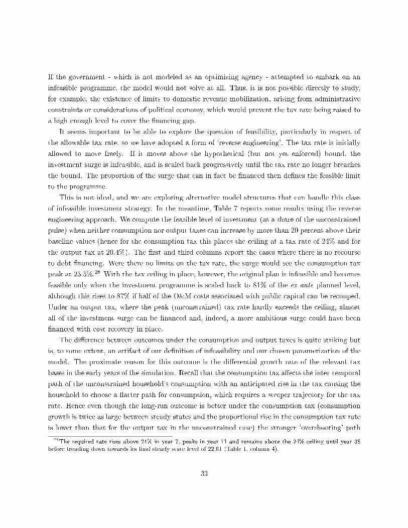
If the government - which is not modeled as an optimizing agency - attempted to embark on an

infeasible programme, the model would not solve at all. Thus, it is not possible directly to study,

for example, the existence of limits to domestic revenue mobilization, arising from administrative

constraints or considerations of political economy, which would prevent the tax rate being raised to

a high enough level to cover the �nancing gap.

It seems important to be able to explore the question of feasibility, particularly in respect of

the allowable tax rate, so we have adopted a form of 'reverse engineering'. The tax rate is initially

allowed to move freely. If it moves above the hypothetical (but not yet enforced) bound, the

investment surge is infeasible, and is scaled back progressively until the tax rate no longer breaches

the bound. The proportion of the surge that can in fact be �nanced then de�nes the feasible limit

to the programme.

This is not ideal, and we are exploring alternative model structures that can handle this class

of infeasible investment strategy. In the meantime, Table 7 reports some results using the reverse

engineering approach. We compute the feasible level of investment (as a share of the unconstrained

pulse) when neither consumption nor output taxes can increase by more than 20 percent above their

baseline values (hence for the consumption tax this places the ceiling at a tax rate of 24% and for

the output tax at 20.4%). The �rst and third columns report the cases where there is no recourse

to debt �nancing. Were there no limits on the tax rate, the surge would see the consumption tax

peak at 25.5%.28 With the tax ceiling in place, however, the original plan is infeasible and becomes

feasible only when the investment programme is scaled back to 81% of the ex ante planned level,

although this rises to 87% if half of the O&M costs associated with public capital can be recouped.

Under an output tax, where the peak (unconstrained) tax rate hardly exceeds the ceiling, almost

all of the investment surge can be �nanced and, indeed, a more ambitious surge could have been

�nanced with cost recovery in place.

The di�erence between outcomes under the consumption and output taxes is quite striking but

is, to some extent, an artifact of our de�nition of infeasibility and our chosen paramerization of the

model. The proximate reason for this outcome is the di�erential growth rate of the relevant tax

bases in the early years of the simulation. Recall that the consumption tax a�ects the inter-temporal

path of the unconstrained household's consumption with an anticipated rise in the tax causing the

household to choose a �atter path for consumption, which requires a steeper trajectory for the tax

rate. Hence even though the long-run outcome is better under the consumption tax (consumption

growth is twice as large between steady states and the proportional rise in the consumption tax rate

is lower than that for the output tax in the unconstrained case) the stronger 'overshooting' path

28The required rate rises above 24% in year 7, peaks in year 11 and remains above the 24% ceiling until year 38before trending down towards its �nal steady state level of 22.61 (Table 1, column 4).

33

of the consumption tax means that the economy is more likely to hit any given tax ceiling on the

dynamic path. Increasing the share of constrained households and/or lowering the inter-temporal

elasticity of substitution in consumption will reduce the di�erence between the consumption tax

and output tax cases.

If the investment surge is debt-�nanced, however, either through non-concessional external

borrowing or domestic bond �nancing, or a mixture of the two, the additional tax burden greatly

compromises the �scal feasibility of the investment programme. For example, with external debt

�nancing, given a constant domestic debt target and no cost recovery, only 53% (60%) of the surge

is feasible under the consumption (output) tax. Substituting (more expensive) domestic for external

debt, as shown in columns 3 and 6, further lowers the feasible size of the investment programme.

TABLE 7: Feasible public investment with tax ceiling.

Baseline settings as Table 1, columns (4) and (8); public investment increased by 3% of GDP

Domestic interest rate 10%; external interest rate 6% + θ(dc/y)


Domestic debt (share of investment surge) 0 0 50 0 0 50

Non-concessional debt (share of investment surge) 0 100 50 0 100 50

Tax ceiling 24.0 24.0 24.0 20.4 20.4 20.4

Maximum unconstrained consumption tax rate 25.5 28.6 26.1

Maximum unconstrained output tax rate 20.8 24.1 22.2

Financeable share of investment (no cost recovery) 81% 53% 47% 98% 60% 45%

Financeable share (50% cost recovery on O&M) 87% 57% 54% 109% 66% 56%


This is, however, only part of the debt �nancing story, since the key function of debt in this

model (and in reality) is that it allows the borrower to break the concurrent (though not the

inter-temporal) link between expenditure and taxation so as to allow for a di�erent inter-temporal

path of taxation. It may be that the government's revenue position (and any associated bound on

tax rates) is expected to ease over time, as a consequence of improvements in tax administration,

the growth of per capita income, or other anticipated events such as increased resource revenues.

Borrowing permits tax rates to be kept down early on, even though the logic of the inter-temporal

budget constraint means they have to rise higher later to cover the debt service, but the future

relaxation in the revenue constraint may now make this feasible. To illustrate the nature of this

inter-temporal trade-o�, Figure 3 plots the di�erent pro�les for consumption and output taxes across

the three scenarios discussed in Table 6. In both cases, although debt �nancing requires higher tax

rates in the new steady state, the short-run pressure on taxation is moderated; taxes rise more

34

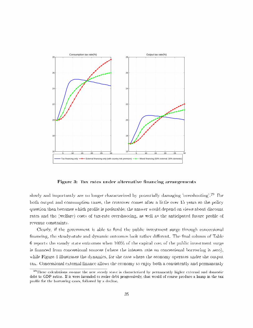
5 10 15 20 25 3016

18

20

22

24

26

28Consumption tax rate(%)

5 10 15 20 25 3016

18

20

22

24

26

28Output tax rate(%)

Tax financing only External financing only (with country risk premium) Mixed financing (50% external ,50% domestic)

Figure 3: Tax rates under alternative �nancing arrangements

slowly and importantly are no longer characterized by potentially damaging 'overshooting'.29 For

both output and consumption taxes, the crossover comes after a little over 15 years so the policy

question then becomes which pro�le is preferable; the answer would depend on views about discount

rates and the (welfare) costs of tax-rate overshooting, as well as the anticipated future pro�le of

revenue constraints.

Clearly, if the government is able to fund the public investment surge through concessional

�nancing, the steady-state and dynamic outcomes look rather di�erent. The �nal column of Table

6 reports the steady state outcomes when 100% of the capital cost of the public investment surge

is �nanced from concessional sources (where the interest rate on concessional borrowing is zero),

while Figure 4 illustrates the dynamics, for the case where the economy operates under the output

tax. Concessional external �nance allows the economy to enjoy both a consistently and permanently

29These calculations assume the new steady state is characterized by permanently higher external and domesticdebt to GDP ratios. If it were intended to retire debt progressively, that would of course produce a hump in the taxpro�le for the borrowing cases, followed by a decline.

35

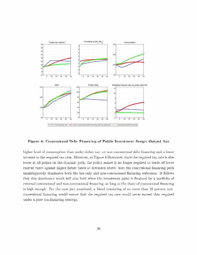
5 10 15 20 25 3012

14

16

18

20

22

24

26

28

30Output tax rate(%)

5 10 15 20 25 30

-4

-3

-2

-1

0

1

2

3

4

Crowding-In [dKp/dK

g]

5 10 15 20 25 3095

100

105

110Consumption

5 10 15 20 25 3095

100

105

110GDP

5 10 15 20 25 300

20

40

60

80

100

120Public Debt

5 10 15 20 25 300

2

4

6

8

10

12

Weighted interest rate on public debt (%)

Tax financing only Non-concessional debt financing (with risk premium) Concessional debt financing

Figure 4: Concessional Debt Financing of Public Investment Surge: Output Tax

higher level of consumption than under either tax- or non-concessional debt-�nancing and a lower

increase in the required tax rate. Moreover, as Figure 4 illustrates, since the required tax rate is also

lower at all points on the dynamic path, the policy maker is no longer required to trade o� lower

current taxes against higher future taxes as discussed above: here the concessional �nancing path

unambiguously dominates both the tax-only and non-concessional �nancing outcomes. It follows

that this dominance result will also hold when the investment pulse is �nanced by a portfolio of

external concessional and non-concessional �nancing, as long as the share of concessional �nancing

is high enough. For the case just examined, a blend consisting of no more than 15 percent non-

concessional �nancing would ensure that the required tax rate would never exceed that required

under a pure tax-�nancing strategy.

36

7 Conclusion

Two staples, both of public �nance theory, and of practical discussions of �scal policy, are that

taxation in�icts deadweight costs, and that public investment imposes ongoing budgetary costs

for operations and maintenance for which provision is often inadequate. The paper by Bu�e

et al sets out to provide a systematic framework for analyzing the interactions between public

investment, �nancing alternatives, the budget, and growth. However, it does not include treatment

of these two issues. This paper extends their model to incorporate them. It is intended to

demonstrate both how this can be done, and to illustrate some of the implications of doing so.

The illustrations, which at this stage are calibrated to the same stylized economy as the original

paper, but which nonetheless result in a plausible representation of the degree of distortion in many

low-income countries, demonstrate both that these extensions have material consequences for the

analysis of the public investment, debt sustainability and growth nexus in low-income countries.

and that the potential payo� to various forms of �scal reform, both tax reforms and reforms to

the institutional arrangements for the budgeting and implementation of O&M expenditures, may

be substantial, both in their own right and in combination with public investment programmes.

Although the results as well as the experiment design remain rather stylized, they point to further

developments of the research that will allow us to bring the model to bear on speci�c country

public investment programmes. Two steps are of primary importance. The �rst involves further

development of the model itself, in particular the introduction of a more nuanced representation

of the tax system, allowing for di�erential taxation of labour and capital income and of di�erent

categories of consumption so that, amongst other things, the model can better analyze real-world

tax reform programmes. This work is well in hand. Second, the current parameterization of O&M

expenditures is based on a combination of Heller's original estimates and simpli�cations implemented

in the interests of model transparency. Further work is therefore required to re-calibrate this part

of the model to (the admittedly still very sparse) contemporary data on actual and 'e�cient'

O&M expenditures. This will require analysis of countries' budgetary and public expenditure

records and of project-based data of the form collected by the World Bank under the aegis of

the Africa Country Infrastructure Diagnostic project (see Foster and Briceno-Garmendia, 2010).

With these developments in hand the modi�ed model will be well-placed to o�er ex ante assessment

of country-speci�c policy programs.

37

References

[1] Auriol, E. and M. Warlters (2012), �The marginal cost of public funds and tax reform in Africa�

Journal of Development Economics 97(1) 58-72.

[2] Barro, R.J. (1990) �Government Spending in a simple model of endogenous growth� Journal of

Political Economy 98(5) s103-26.

[3] Barro, R.J. and X. Sala-i-Martin (1992), �Public �nance in models of economic growth� Review

of Economic Studies 59(4), 645-61.

[4] Berg, A., S. Yang and L-F. Zanna (2014) �Modeling African Economies: A DSGE Approach�

(mimeo, IMF)

[5] Bu�e, E., A. Berg, C. Pattillo, R. Portillo and L-F. Zanna (2012) �Public investment, growth,

and debt sustainability: putting together the pieces.� IMF Working Paper WP12/144.

[6] Fay, M. and T. Yepes (2003) �Investing in Infrastructure: What is Needed from 2000 to 2010?�

World Bank WPS 3102.

[7] Foster, V. and C. Briceno-Garmendia (2010) Africa's Infrastructure: a Time for Transition

World Bank, Washington DC.

[8] Gray, C. and A. Martens (1983) �The Political Economy of the 'Recurrent Cost Problem' in

the West African Sahel� World Development 11(2), 101-117.

[9] Heller, P.S. (1974) �Public Investment in LDC's with Recurrent Cost Constraint: the Kenyan

case� Quarterly Journal of Economics 88(May), 251-77.

[10] Heller, P.S. (1991) �Operations and Maintenance� IMF Public Expenditure Handbook IMF,

Washington DC.

[11] Keen, M. (2012) �Taxation and Development - Again� IMF Working Paper WP/12/220.

[12] Kloeden, D. (2011) �Revenue Administration Reforms in Anglophone Africa Since the Early

1990s� IMF Working Paper WP/11/162.

[13] Rioja, F.K. (2003) �Filling potholes: macroeconomic e�ects of maintenance versus new

investments in public infrastructure� Journal of Public Economics 87, 2281-2304.

[14] Sunderland, D. (2007) �Managing British Colonial and Post-Colonial Development: The Crown

Agents, 1914-1974� Boydell Press, Woodbridge.

38

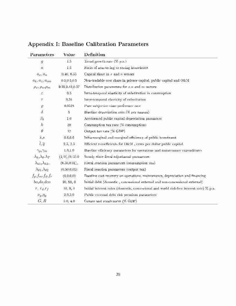
Appendix I: Baseline Calibration Parameters

Parameters Value De�nition

g 1.5 Trend growth rate (% p.a.)

a 1.5 Ratio of non-saving to saving households

ax, an 0.40, 0.55 Capital share in x and n sectors

ak, az, aom 0.5,0.5,0.5 Non-tradable cost share in private capital, public capital and O&M

ρx, ρn,ρm 0.20,0.43,0.37 Distribution parameters for x,n and m sectors

ε 0.5 Intra-temporal elasticity of substitution in consumption

τ 0.34 Inter-temporal elasticity of substitution

% 0.0528 Pure subjective time preference rate

δ 5 Baseline depreciation rate (% per annum)

βδ 1.0 Accelerated public capital depreciation parameter

h 20 Consumption tax rate (% consumption)

θ 17 Output tax rate (% GDP)

s,s 0.6,0.6 Infra-marginal and marginal e�ciency of public investment

l, q 2.5, 2.5 E�cient r-coe�cients for O&M , cents per dollar public capital.

γp,γm 1.0,1.0 Baseline e�ciency parameters for operations and maintenance expenditures

λh,λθ,λT (1/0),(0/1),0 Steady state �scal adjustment parameters

λh1,λh2, (0.50,0.01), Fiscal reaction parameters (consumption tax)

λθ1,λθ2 (0.50,0.01) Fiscal reaction parameters (output tax)

fp,fm,fd,fr (0,0,0,0) Baseline cost recovery on operations, maintenance, depreciation and �nancing

bo,do,dco 20, 50, 0 Initial debt (domestic , concessional external and non-concessional external)

r, rd,rf 10, 0, 4 Initial interest rates (domestic, concessional and world risk-free interest rate) % p.a.

νg,ηg 2.0,3.0 Public external debt risk premium parameters

G,R 5.0, 4.0 Grants and remittances (% GDP)

39

Appendix II: Cost recovery and incomplete appropriability

Assume that the public capital stock grows at the steady rate g, that debt service on a unit of

borrowing is dt after time t, and that this is arranged to fall at the constant rate φ, so that for a dollar

loan taken out at time 0, dt = d0e−φt. Also assume for the moment that the investment programme

is entirely �nanced by borrowing; then, if the government's cost of borrowing is stationary at i, it

follows that d0 = i + φ. Let the public capital stock be K0 at time 0, so that gross investment, to

cover both depreciation and the required net growth, is (g + δ)K0. It is then straightforward to

show that, integrating over past investment, the payment to cover debt service on this cumulated,

depreciated, investment at time 0 is:

(i+ φ)(g + δ)K0

(g + φ)

To avoid a budgetary drain, the user charge (R) would have to be set to cover this cost as well

as the O&M costs (r per unit of capital). In other words:

R ≥(r +

(i+ φ)(g + δ)

(g + φ)

)Note that if the interest rate exceeds the growth rate, it is helpful to pay o� the debt rapidly:

if the growth rate exceeds the interest rate, it pays to do the reverse. Now consider the plausible

scenario in which debt service on a particular loan is set to fall at the same rate as the rate of

depreciation of the capital it was used to �nance, so that φ = δ.Then the requirement simpli�es

to R ≥ (r + i + δ).To avoid a drain, the budgetary return to capital needs to be at least equal to

the sum of the r-coe�cient, the interest rate, and the depreciation rate. For example, suppose the

r-coe�cient is 0.1, the real interest rate is 10%, and the depreciation rate is 5%. Then to prevent

part of these costs becoming a burden on the budget, cost recovery will have to yield a gross return

on capital of at least 25% per annum. This argument might appear to rely on the whole investment

being �nanced by borrowing. However, even if part of the initial cost was tax �nanced, that revenue

has an opportunity cost; in the absence of the investment, it could have been used to reduce public

debt, and the government's borrowing rate is again a measure of this opportunity cost.

In these circumstances, the ratio of outstanding debt to the capital stock is stationary, whatever

the value of φ. However, only when φ = δ is the stationary ratio of the debt stock the same as

the proportion of investment �nanced by borrowing. It seems reasonable that, if a government was

content to �nance x% of its current investment by borrowing, it should be content that its debt to

capital ratio should also be x%, and that is achieved by setting φ = δ.

40

The problem of incomplete appropriability arises when a project generates a social return in

excess of (r+ i+ δ), so is in principle worth carrying out, but cost recovery can only be achieved at

a level below (r + i+ δ), so that the project imposes a net budgetary cost. A decision then has to

be made, given an estimate of the MCF, and/or the existence of bounds on achievable tax rates, as

to whether the project should still be undertaken.

Finally, it is important to realize that this modeling of the �nancing costs seeks to focus on what

the budgetary authorities ought to have in mind either in setting targets for user charges to cover

these costs, or in facing up to the budgetary implications of failing to do so. The actual pattern

of borrowings, interest payments and repayments is a separate issue, and the dynamic model picks

these up in whatever detail the model user provides.

41

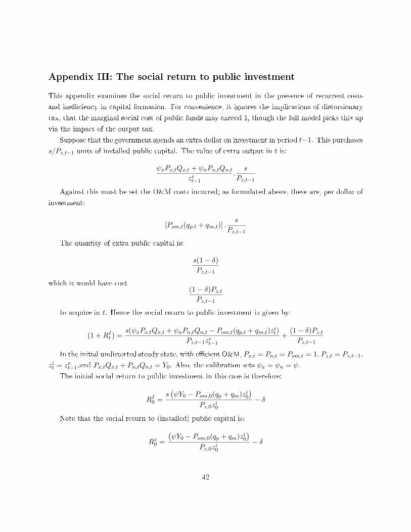
Appendix III: The social return to public investment

This appendix examines the social return to public investment in the presence of recurrent costs

and ine�ciency in capital formation. For convenience, it ignores the implications of distortionary

tax, that the marginal social cost of public funds may exceed 1, though the full model picks this up

via the impact of the output tax.

Suppose that the government spends an extra dollar on investment in period t−1. This purchases

s/Pz,t−1 units of installed public capital. The value of extra output in t is:

ψxPx,tQx,t + ψnPn,tQn,tzet−1

.s

Pz,t−1

Against this must be set the O&M costs incurred; as formulated above, these are, per dollar of

investment:

[Pom,t(qp.t + qm,t)] .s

Pz,t−1

The quantity of extra public capital is:

s(1− δ)Pz,t−1

which it would have cost(1− δ)Pz,tPz,t−1

to acquire in t. Hence the social return to public investment is given by:

(1 +RIt ) =s(ψxPx,tQx,t + ψnPn,tQn,t − Pom,t(qp,t + qm,t)z

it)

Pz,t−1zet−1

+(1− δ)Pz,tPz,t−1

In the initial undistorted steady state, with e�cient O&M, Px,t = Pn,t = Pom,t = 1, Pz,t = Pz,t−1,

zit = zet−1,and Px,tQx,t + Pn,tQn,t = Y0. Also, the calibration sets ψx = ψn = ψ.

The initial social return to public investment in this case is therefore:

RI0 =s(ψY0 − Pom,0(qp + qm)zi0

)Pz,0zi0

− δ

Note that the social return to (installed) public capital is:

Rz0 =

(ψY0 − Pom,0(qp + qm)zi0

)Pz,0zi0

− δ

42

Having s < 1 in�icts a double hit in lowering the return to investment relative to the return to

capital. First, it lowers the gross of depreciation return by the factor s, but, second, the deduction for

depreciation to get the net return is una�ected, rather than being similarly reduced. For example,

let(ψY0/Pz,0z

i0

)= 0.30, (Pom,0(qp + qm)) /Pz,0 = 0.05, δ = 0.05, and s = 0.6. Then Rz0 = 0.35 −

0.05−0.05 = 0.25. But RI0 = 0.6∗(0.35−0.05)−0.05 = 0.18−0.05 = 0.13. The gross of depreciation

rate falls to 60% of the e�cient value (0.18/0.30), but the net rate falls to only 52% of the e�cient

value (0.13/0.25).

43

Public Investment, Public Finance, and Growth: The Impact ... · PDF fileWP/14/73 Public...

Documents

Transcript of Public Investment, Public Finance, and Growth: The Impact ... · PDF fileWP/14/73 Public...