Public insurance and private savings: who is affected and by how much?
27
JOURNAL OF APPLIED ECONOMETRICS J. Appl. Econ. 24: 282–308 (2009) Published online 12 November 2008 in Wiley InterScience (www.interscience.wiley.com) DOI: 10.1002/jae.1039 PUBLIC INSURANCE AND PRIVATE SAVINGS: WHO IS AFFECTED AND BY HOW MUCH? ALEX MAYNARD a * AND JIAPING QIU b a Department of Economics, University of Guelph, Ontario, Canada b DeGroote School of Business, McMaster University, Hamilton, Ontario, Canada SUMMARY This paper employs a recently developed instrumental quantile regression method to investigate the effect of Medicaid on household savings across different wealth groups. It finds that the disincentive effect of Medicaid on household savings is heavily concentrated in the middle net-worth households. In contrast, the effects on the bottom and top net-worth households are quite small and insignificant. These heterogeneous incentive effects are partly explained by Medicaid asset tests. Our findings hold regardless of whether affluence is measured in terms of wealth or income. They suggest that despite generating substantial crowd-out for the mean household, Medicaid expansions are unlikely to discourage the savings of the poorest households. Copyright 2008 John Wiley & Sons, Ltd. 1. INTRODUCTION A central question concerning public insurance programs is the extent to which they crowd out private savings. Government insurance plans, such as Medicaid or Aid to Families with Dependent Children (AFDC), may crowd out savings in two primary ways. First, by insuring households against out-of-pocket medical expenses or income shocks, public insurance programs may reduce the household’s reliance on precautionary savings as an alternative form of insurance, as suggested by the simulation results in Kotlikoff (1989). Secondly, as demonstrated by Hubbard et al. (1995), asset test eligibility requirements act as an implicit tax on wealth and may encourage households to spend down assets in order to qualify for public insurance programs. 1 The effect of public insurance on private savings has been an active area of empirical research (e.g., Starr-McCluer, 1996; Palumbo, 1999; Chou et al., 2003; Powers, 1998). Using the quasi- exogenous component of the variation from the expansion of Medicaid coverage, Gruber and Yelowitz (1999) find empirical support for the contention that, on average, an increase in a household’s Medicaid coverage leads to a reduction in household wealth and that this effect is magnified in the presence of an asset test. A recent study by Hurst and Ziliak (2006) uses the 1996 Welfare reform to test whether welfare asset limits serve as a deterrent to savings for poor households. Interestingly, they find no effect of the welfare policy changes, which relaxed asset Ł Correspondence to: Alex Maynard, Department of Economics, University of Guelph, McKinnan Building, Guelph, Ontario, Canada N1G 2W1. E-mail: [email protected] 1 Since public insurance programs provide an in-kind transfer payment, the associated wealth effect provides a third channel whereby public insurance may affect savings. Copyright 2008 John Wiley & Sons, Ltd.
-
Upload
alex-maynard -
Category
Documents
-
view
213 -
download
0
Transcript of Public insurance and private savings: who is affected and by how much?

JOURNAL OF APPLIED ECONOMETRICSJ. Appl. Econ. 24: 282–308 (2009)Published online 12 November 2008 in Wiley InterScience(www.interscience.wiley.com) DOI: 10.1002/jae.1039
PUBLIC INSURANCE AND PRIVATE SAVINGS: WHO ISAFFECTED AND BY HOW MUCH?
ALEX MAYNARDa* AND JIAPING QIUb
a Department of Economics, University of Guelph, Ontario, Canadab DeGroote School of Business, McMaster University, Hamilton, Ontario, Canada
SUMMARYThis paper employs a recently developed instrumental quantile regression method to investigate the effect ofMedicaid on household savings across different wealth groups. It finds that the disincentive effect of Medicaidon household savings is heavily concentrated in the middle net-worth households. In contrast, the effects onthe bottom and top net-worth households are quite small and insignificant. These heterogeneous incentiveeffects are partly explained by Medicaid asset tests. Our findings hold regardless of whether affluence ismeasured in terms of wealth or income. They suggest that despite generating substantial crowd-out for themean household, Medicaid expansions are unlikely to discourage the savings of the poorest households.Copyright 2008 John Wiley & Sons, Ltd.
1. INTRODUCTION
A central question concerning public insurance programs is the extent to which they crowd outprivate savings. Government insurance plans, such as Medicaid or Aid to Families with DependentChildren (AFDC), may crowd out savings in two primary ways. First, by insuring householdsagainst out-of-pocket medical expenses or income shocks, public insurance programs may reducethe household’s reliance on precautionary savings as an alternative form of insurance, as suggestedby the simulation results in Kotlikoff (1989). Secondly, as demonstrated by Hubbard et al. (1995),asset test eligibility requirements act as an implicit tax on wealth and may encourage householdsto spend down assets in order to qualify for public insurance programs.1
The effect of public insurance on private savings has been an active area of empirical research(e.g., Starr-McCluer, 1996; Palumbo, 1999; Chou et al., 2003; Powers, 1998). Using the quasi-exogenous component of the variation from the expansion of Medicaid coverage, Gruber andYelowitz (1999) find empirical support for the contention that, on average, an increase in ahousehold’s Medicaid coverage leads to a reduction in household wealth and that this effectis magnified in the presence of an asset test. A recent study by Hurst and Ziliak (2006) uses the1996 Welfare reform to test whether welfare asset limits serve as a deterrent to savings for poorhouseholds. Interestingly, they find no effect of the welfare policy changes, which relaxed asset
Ł Correspondence to: Alex Maynard, Department of Economics, University of Guelph, McKinnan Building, Guelph,Ontario, Canada N1G 2W1.E-mail: [email protected] Since public insurance programs provide an in-kind transfer payment, the associated wealth effect provides a thirdchannel whereby public insurance may affect savings.
Copyright 2008 John Wiley & Sons, Ltd.

PUBLIC INSURANCE AND PRIVATE SAVINGS 283
test limits, on the savings of female-headed households with children, a demographic group whichtends to be at risk of taking up welfare and thus would seem likely to respond to the policy reform.
The fact that the savings effect of public insurance may vary across households of differentwealth or income levels is suggested by the theoretical contributions of Hubbard et al. (1995),who argue that public insurance, in combination with an asset test, provides stronger savingsdisincentives to low-than to high-income households. They use this heterogeneity to explain thesharp and rather puzzling disparity of savings rates observed across wealth and income groups.Most of the public insurance programs, such as Medicaid and AFDC, were originally designedas safety nets for poor households. Savings rates among these groups are already quite low.Thus, although the welfare implications are uncertain,2 to the extent that the savings crowd-outis concentrated among poor households, this may be of particular concern to policy makers. AsSherraden (1991) argues, savings are of crucial importance to the long-run economic status ofpoor households. With limited ability to borrow, a lack of savings may force these householdsto forgo important investments in education or down payments on home or business ownership.Ultimately, this may make it more difficult for the family, as well as their offspring, to exit frompoverty.
Therefore, both economic and policy considerations suggest the importance of examiningthe disincentive effects of public insurance programs across different segments of the wealthdistribution. Employing the data on the expansion of Medicaid in the late 1980s/early 1990s thatGruber and Yelowitz (1999) use to study population average effects, we ask whose savings areaffected by Medicaid and by how much. Specifically, we investigate the effect of Medicaid onsavings across households with different wealth levels, using a recently developed instrumentalvariable quantile regression approach. In this way, we can directly measure the savings effect ofMedicaid on the poorest households, who make the greatest use of Medicaid and whose savingsare lowest. Moreover, this allows us to assess the empirical predictions of Hubbard et al. (1995)on the differential effect of Medicaid asset tests across households of different means.
Our study yields interesting empirical results. We find a strong negative impact of Medicaidcoverage on median household wealth. We also find that the effect dissipates as we move into thetop quantiles and becomes insignificant in the top decile. This is an expected result that follows theprediction of Hubbard et al. (1995). In fact, if the results for the upper quantiles hold any surprise,it is rather that response does not dissipate more quickly. Perhaps most interestingly, the effectagain dissipates in the lower quantiles. In fact, for the poorest households, who have the highestparticipation rates in Medicaid, there is no evidence that Medicaid has any impact whatsoever onhousehold asset accumulation. As we argue below, this could be due to the fact that the net worthof the poorest households lies safely below asset test thresholds and their consumption–savingschoices may also be restrained by credit constraints.
We explore the explanation behind the heterogeneous savings effects uncovered here. Thedifferential impact of asset testing across net worth quantiles is found to be an important componentto this explanation. Like Medicaid spending itself, we find that Medicaid asset tests also have noeffect on the top and bottom net worth quantiles. The effect is strongest for the lower middlequantiles. For these households, asset levels tend to be only a few thousand dollars above theeligibility ceilings. Thus, any policy or family structure change that leads them to become eligibleon other grounds creates a strong savings disincentive in order to meet the asset test. By contrast,
2 Unlike the savings reductions due to Medicaid asset tests, reductions in precautionary savings may not cause distortions,as precautionary saving is itself an inefficient form of savings.
Copyright 2008 John Wiley & Sons, Ltd. J. Appl. Econ. 24: 282–308 (2009)DOI: 10.1002/jae

284 A. MAYNARD AND J. QIU
households in the top quantiles would have to spend down substantial assets in order to qualify forMedicaid. As argued by Hubbard et al. (1995), they are unlikely to find this an attractive option.Finally, the households in the bottom quantiles have few savings to begin with and thus qualifyautomatically on asset test grounds, without any need to further reduce their asset holdings.
Nevertheless, we find that the differential incentives caused by asset testing can explain onlypart of the overall heterogeneity in the savings response to Medicaid. Even in the absence of anasset test, the effect of Medicaid on savings still varies considerably across quantiles. This suggeststhat the strength of a household’s precautionary savings response to Medicaid also depends on itswealth level. In particular, households in the middle quantiles may have substantial precautionarysavings reserved for use in the event of a medical emergency, prior to their enrollment in Medicaid.After meeting eligibility requirements, such precautionary savings may no longer be necessary,suggesting a sharp drop in net assets. By contrast, the very poorest households have little to noprecautionary savings, regardless of whether they are eligible for Medicaid. Medical emergenciesoften entail large discrete costs, such as hospital stays, and, with limited economic opportunities,many of these households may have little prospect of accumulating sufficient net worth toprovide useful levels of precautionary medical savings in the absence of Medicaid. Similarly,they may not be able to increase consumption much in the presence of Medicaid due to creditconstraints.
In the quantile regression results discussed above, poverty is implicitly defined in terms of networth. However, it is possible that some households may have high incomes but few assets orvice versa. Examples would include newly minted doctors or lawyers with high starting salariesbut large student loans or a head of household facing a long stretch of unemployment after manyyears of high salary and savings. Therefore, we also examine the savings disincentive effectsof Medicaid and asset testing across the quantiles of labor income. This analysis indicates thatMedicaid has no effect on the bottom and top 20% of households as measured by labor income.Therefore, the same general conclusions hold regardless of whether we define poverty in terms ofassets or income.
Our findings have several important implications. Medicaid has traditionally targeted poorhouseholds, for whom savings rates are quite low. Although the welfare effects are uncertain,any tendency to further crowd out these already low savings may still be of concern in a programdesigned to address poverty. Yet, we find no evidence to suggest that Medicaid discouragessavings among the poorest households. Thus, among this demographic, any ex ante Medicaidsavings disincentives for healthy households appear second order relative to the ex post benefitsassociated with Medicaid coverage for households with disability or long-term illness.
Secondly, our findings potentially reconcile some of the results of the previous literature.For example, focusing on female-headed households with children, a disproportionately poorpopulation, Hurst and Ziliak (2006) find no evidence that asset tests affect savings, whereasGruber and Yelowitz (1999) find evidence of a strong effect when averaged across the positivenet worth Survey of Income and Program Participation (SIPP) population. Our results, which findno savings effects for households towards the bottom of the wealth distribution, yet strong effectsfor the median household, are consistent with the findings of both studies. More generally, thissuggests that the conclusions obtained from population average studies may show some sensitivityto the income and/or wealth composition of the sample employed. In fact, when controlling forlabor income, we also find that both the estimate and significance of the mean savings responsein the SIPP is sensitive to the inclusion of non-positive net worth households.
Copyright 2008 John Wiley & Sons, Ltd. J. Appl. Econ. 24: 282–308 (2009)DOI: 10.1002/jae

PUBLIC INSURANCE AND PRIVATE SAVINGS 285
Our study also sheds some light on the ability of public insurance programs to explain thepuzzling low savings rates among the poorest households. Standard consumption smoothing modelstend to have difficulty explaining the difference in savings rates between low-and high-incomehouseholds. This suggests that heterogeneity of some form is likely important in resolving thispuzzle. Public insurance programs, which are relevant to poor, but not to wealthy households,thus provide a promising explanation (Hubbard et al., 1995). Our results are supportive of thisexplanation in so far as it applies to the moderately poor households in the lower middle net worthquantiles. On the other hand, we do not find any evidence that public insurance helps to explainthe abnormally low savings rates found among the very poorest households. Simply put, thesehouseholds do not appear to maintain any significant savings, regardless of whether or not theyare on Medicaid.
Finally, our results imply that the percentage savings response to a one-dollar increase inMedicaid for a household in the eighth net worth decile is approximately the same as that ofa household in the third decile. This comparison is particularly stark when measured in dollarsavings responses, but seems somewhat less severe when viewed as elasticities. To the extent thatthe estimated saving disincentive effects in the upper-middle deciles (6–8) seem large relative toprior beliefs, they may suggest some caution regarding the empirical specification and thereforethe causal inference that Medicaid affects savings.3 We discuss this caveat further in Section 3.2.
The rest of the paper proceeds as follows. Section 2 describes the data and methodology. Section3 presents and explains the empirical results, and Section 4 summarizes and concludes.
2. DATA AND METHODOLOGY
2.1. Data
In this study, we employ data from the Survey of Income and Program Participation (SIPP),spanning 1984–1993. The SIPP consists of a series of overlapping panels initiated on a yearly basis,but lasting for a total of 24–32 months, during which time the same households are repeatedlyinterviewed at 4-month intervals in order to collect data on household income and Medicaidparticipation.
Data on household net worth was collected from each household as part of a special topicalmodule. Net worth is defined as the sum of financial assets and home, vehicle, and business equity,net of debt. In the SIPP database, assets are defined to include interest-earning assets,4 stocks andmutual fund shares, mortgages held from the sale of real estate, amount due from sale of businessor property, regular checking accounts, US Savings Bonds, real estate, IRAs and KEOGH accounts,and motor vehicles. Debts include both secured debt (mortgages, business or professional debt,vehicle loans, and margin and broker accounts) and unsecured debt (credit card and store bills,medical bills, educational loans, and loans from individuals and financial institutions).
Following Gruber and Yelowitz (1999), we employ the wealth information for each householdfrom the special topical module, together with an average of the other household characteristicsobtained from the interviews for that household prior to and including the wealth module. Thus,
3 We thank an anonymous referee for pointing this out.4 These include passbook savings accounts, money market funds, deposit accounts, certificates of deposit, interest earningchecking accounts, US government securities, and municipal and corporate bonds.
Copyright 2008 John Wiley & Sons, Ltd. J. Appl. Econ. 24: 282–308 (2009)DOI: 10.1002/jae

286 A. MAYNARD AND J. QIU
we employ a pooled cross-section with one observation for each household, spanning 10 yearsand 52,706 households, of which 40,442 have positive net worth.5,6
This is a particularly interesting period in which to study the effects of Medicaid. Prior to 1984,Medicaid had strict income and asset requirements, and was limited to female-headed householdsreceiving welfare benefits through the Aid to Families with Dependent Children (AFDC) program.However, over the next decade, Medicaid underwent a number of expansions, which relaxedfamily structure, income, and asset eligibility requirements. This policy change was the resultof separate legislative changes passed and implemented over several years and thus providessubstantial variability in Medicaid benefits across the time series dimension of the data. Althoughthe changes occurred at the federal level, the legislation left the states considerable flexibility asto the speed and, to some extent, the depth of the expansion. States also varied widely accordingto the age cut-off for children’s eligibility. Therefore, these changes also gave rise to considerablevariability across states. More importantly for our study, even within the same state and year,the value of the eligibility expansion varied considerably across households, depending on thehousehold family structure, age, and the local cost of medical services. The reader is referredto Gruber and Yelowitz (1999) and Currie and Gruber (1996a,b) for a detailed account of theseexpansions.
2.2. Methodology
Our primary interest lies in the response of household net worth to changes in the value ofthe Medicaid subsidy, which reflect changes to both Medicaid eligibility and generosity. Thedependent variable, net worth, is directly available from SIPP. The primary regressor, Medicaideligible dollars (MED), is a carefully constructed measure of the household’s expected Medicaidsubsidy proposed by Gruber and Yelowitz (1999) and Currie and Gruber (1996a,b). This measuretakes into account variation at the household level in both the probability of Medicaid eligibility(due to differences in family structure, income, assets, and eligibility requirements) and expectedhealth care costs (as a function of family composition, age, and state-specific medical costs). Thefull value of Medicaid to a household includes its value in both current and future years. Theexpected Medicaid benefit for family j in year t with family members indexed by i is thereforedefined as the discounted sum of expected future Medicaid benefits:7
MEDj,t D1∑
sD0
�1 C r��s∑
i
ELIGi,j,tCs ð SPENDi,j,tCs �1�
where ELIGi,j,tCs is the probability in year t that family member i is eligible for Medicaid inyear t C s, conditional on the continuation of the Medicaid eligibility rules in place in year t,SPENDi,j,tCs is the expected Medicaid subsidy conditional on eligibility, and r is the real interestrate set to 6%.
5 Households with imputed net worth (about 1/4 of households) are excluded from the sample on account of the reportedproblems with this imputation method (Curtin et al., 1989; Hurd et al., 1998). Likewise, the sample was restricted toheads of household aged 16–64 and a maximum household age of 64, in order to exclude Medicare recipients. Alsoomitted were households containing more than one family. See Gruber and Yelowitz (1999) for further details.6 Note that this pooled cross-section differs from a panel in that different households’ wealth information is sampled atdifferent points in time.7 Note that the expectations are implicit in the definitions of SPEND and ELIG.
Copyright 2008 John Wiley & Sons, Ltd. J. Appl. Econ. 24: 282–308 (2009)DOI: 10.1002/jae

PUBLIC INSURANCE AND PRIVATE SAVINGS 287
As discussed above, the large but uneven expansion of Medicaid gives rise to substantialvariation in both Medicaid eligibility and the expected value of Medicaid to households. However,this variability must be employed with care since policy changes are not true natural experimentsand some of this variation is likely endogenous. One potential source of endogeneity mayarise from the effects of lobbying or other political pressures affecting policy. This suggestscorrelation between policy changes and average yearly household characteristics due to politicaleconomy considerations at the federal level, and between policy and average state–year householdcharacteristics due to lobbying at the state level. Therefore, the exogeneity of policy changes acrossboth states, years, and state–year cells is questionable. For this reason, it seems preferable to focuson the within-state–year cell variability in Medicaid eligible dollars. This variation arises fromthe fact that the same policy change may have substantially different effects on eligibility acrosshouseholds due to the interaction between the policy change and the household characteristics.By including a full set of year, state, and year–state interaction dummy variables to absorb thevariation across year–state cells, we follow Gruber and Yelowitz (1999) in employing only thiswithin-cell variation.
A second potential source of endogeneity arises from the fact that eligibility also dependson both wealth levels (via asset tests) and income levels (via income tests), which themselvesdepend in part on net worth. This suggests that a substantial portion of the variability in eligibilitymay be endogenous and thus MED requires an instrument. A natural instrument in this contextis the exogenous component to Medicaid eligible dollars. This is constructed in Gruber andYelowitz (1999) as a second measure of expected Medicaid subsidies, simulated Medicaid eligibledollars (SIMMED), in which the probability of eligibility is conditioned on what they argueto be the factors determined exogenously to current savings decisions: education, age, state,and year. To be precise, the probability of eligibility, ELIG in (1), is replaced by SIMELIG,in which this probability is simulated using only the exogenous factors discussed above. Then,the expected Medicaid benefit for family j in year t conditional on exogenous factors only isgiven by
SIMMEDj,t D1∑
sD0
�1 C r��s∑
i
SIMELIGi,j,tCs ð SPENDi,j,tCs
which is defined in the same way as MED in (1), except that ELIG is replaced by SIMELIG.To examine the effect of Medicaid across different segments of wealth distribution, we employ
a quantile regression approach, which allows us to estimate the marginal effect of a givenMedicaid expansion for households at different points in the conditional wealth distribution. Thismakes it possible to separately assess the implication of Medicaid reform for poor, middle-class, and wealthy households. Since Medicaid eligible dollars requires an instrument, weemploy the instrumental variable quantile regression approach of Chernozhukov and Hansen(2004b, 2005). This method, which we briefly describe in the following section, provides oneof several recent solutions to the long-standing problem of quantile regression with endogenousregressors.8
Accordingly, the baseline specification consists of an instrumental quantile regression of log networth on Medicaid eligible dollars, together with a large number of control variates to account
8 See also Powell (1983), Chen and Portnoy (1996), Alberto et al. (2002), Chesher (2003), Ma and Koenker (2006),Chernozhukov and Hansen (2006), and Horowitz and Lee (2007) for alternative solutions to related problems involvingendogeneities in quantile regression.
Copyright 2008 John Wiley & Sons, Ltd. J. Appl. Econ. 24: 282–308 (2009)DOI: 10.1002/jae

288 A. MAYNARD AND J. QIU
for the other factors that enter the savings decision. These include state, year, and state–yearinteraction dummy variables and controls for education, family demographic structure and otherhousehold covariates.
2.3. Instrumental Quantile Regression
2.3.1 Quantile RegressionThe quantile regression, introduced by Koenker and Bassett (1978), estimates the � quantile,QY��jx�, of Y, conditional on X D x, where �ε�0, 1� indexes the quantile level and where capitalletters denote random variables and lower-case letters denote their realizations. In a linear quantileregression model, this is specified as QY��jx� D x0����. Under the asymmetric absolute deviationloss function ���u� D u�� � 1�u < 0��, Koenker and Bassett (1978) show that the expected loss isminimized by the conditional quantile QY��jx�. The quantile regression coefficients O���� are thenchosen to minimize the finite sample analog 1
n∑n
iD1 ���Yi � X0i��. For example, �1/2�u� D 1/2juj
is used for Laplace’s median regression function.The quantile regression is robust to the outliers that are often present in data on wealth. Most
importantly for our study, it offers a rich description of the manner in which the regressors influencethe dependent variable. Rather than restricting the influence of X to shifts in the conditional meanof Y, it allows for differential effects of X at different points in the distribution of Y. This isbecause the coefficients ���� are allowed to vary in a flexible manner according to the quantilelevel �. In particular, a linear quantile regression estimates the model
Y D X0��U� �2�
whereUjX ¾ Uniform(0,1) �3�
and Qy��jx� D x0���� is by design the � quantile of Y conditional on X D x. This provides aflexible description of the conditional distribution function.
In contrast, the standard regression model with homoscedastic errors restricts the influence of theregressors to parallel shifts in the distribution function, in which they have the same influence acrossthe entire distribution. In the current context, standard regression assumptions require Medicaidto have the same expected impact on the wealthiest household in the sample as on the poorest,whereas quantile regression allows us to estimate the impact on the wealthy separately from theimpact on the poor.
2.3.2 Instrumental Quantile RegressionWhen its econometric assumptions are satisfied, the model in (2)–(3) provides a causal interpre-tation for the quantile coefficients ����, which represent the effect of a one-unit change in theregressor on the � quantile of Y. The key identifying assumption underlying this interpretation isthe condition in (3) requiring the error term U to be independent of X. When one or more of theregressors is endogenous, this condition is violated. While the conditional quantile function canthen still be estimated as a descriptive statistic, it loses its causal interpretation. This is the case inthe current study since, as discussed above, Medicaid eligible dollars are endogenous and requirean instrument.
Copyright 2008 John Wiley & Sons, Ltd. J. Appl. Econ. 24: 282–308 (2009)DOI: 10.1002/jae

PUBLIC INSURANCE AND PRIVATE SAVINGS 289
We therefore employ the instrumental quantile regression of Chernozhukov and Hansen (2004b,2005). Denoting the endogenous regressors by D, the included exogenous regressors by X, andthe excluded exogenous instruments by Z, we estimate the structural quantile regression model:9
Y D D0˛�U� C X0ˇ�U� �4�
UjX, Z ¾ Uniform(0,1) �5�
D D υ�X, Z, V� �6�
The identifying assumption in (5) requires that U be independent of both X and Z, but there isno restriction on the dependence between U and V, the potentially endogenous component to D.
The interpretation of coefficients ˛��� and ˇ��� in (4) differs from those of the traditionalquantile regression coefficients, ���� in (2). In particular, they no longer describe the quantilefunction of the observed value of Y conditional on D, and X, a quantile function which confoundsthe influences of D and U in the presence of endogeneity. The coefficients ˛��� can instead beinterpreted as describing the hypothetical impact of an exogenous change in D on the quantiles ofY. This interpretation is formalized by defining the potential or latent outcome of Y for any givenfixed value of d as
Yd D d0˛�U� C X0ˇ�U� UjX, Z ¾ Uniform(0,1) �7�
The coefficients in ˛��� and ˇ��� can then be seen as describing the conditional quantile functionof the potential outcome Yd conditional on X, which Chernozhukov and Hansen (2004b, 2005)define as the structural quantile function, sY��jd, x�. They model it linearly as
sY��jd, x� D d0˛��� C x0ˇ��� �8�
Because d is fixed, the conditional (on X) quantile function of the latent outcomes Yd in(7) captures the effect of d on Y, uncontaminated by any feedback.
Since Yd is latent, the structural quantile function sY��jd, x� cannot be estimated directly byquantile regression. However, under suitable regularity conditions, Chernozhukov and Hansen(2005) show that it may be identified by the conditional moment condition
P[Y � sY��jD, X�jZ, X] D � �9�
using the instrument Z. The instrumental quantile regression of Chernozhukov and Hansen (2004b),which we employ below, provides a clever method of estimating the structural quantile using therestriction in (9). Moreover, their results apply also to the case in which the original instrumentZ is replaced by the fitted value from a standard first-stage linear regression of D on X and Z.
Although our study is the first to apply quantile regression methods to study the impactof Medicaid on savings behavior, quantile regression methods have recently been employedin a number of papers that consider the effect of government policy on savings incentives.
9 Although this is referred to as a structural quantile model, we have not explicitly derived our specification from aneconomic model and therefore our use of this method may also be viewed as a quantile regression analog to reduced-forminstrumental variable regression.
Copyright 2008 John Wiley & Sons, Ltd. J. Appl. Econ. 24: 282–308 (2009)DOI: 10.1002/jae

290 A. MAYNARD AND J. QIU
Employing eligibility as an instrument for participation, Chernozhukov and Hansen (2004a) applythe instrumental quantile regression described above to analyze the impact of 401(K) retirementplans on savings. Using standard quantile regression, Chou et al. (2003) study the savings effectof the introduction of National Health Insurance in Taiwan in 1995. Given the absence of meanstests, their study isolates the precautionary savings motive. Cagetti (2003) matches the parametersfrom a median regression to a wealth accumulation model with precautionary and retirementmotives. He finds that households are impatient but risk averse and concludes that most savingsare precautionary until age 45. Quantile regressions have also been employed in other contextsusing data on wealth and savings, particularly to study wealth gaps, including those between racialgroups (Hurst et al., 1998), across regions (Conley and Galenson, 1994, 1998), between nativesand immigrants (Cobb-Clark and Hildebrand, 2006), and between cohorts (Kapteyn et al., 2005).
3. EMPIRICAL RESULTS
3.1. Summary Statistics of Household Characteristics across Net Worth Quantiles
We focus first on households with positive net worth, both because we are particularly interestedin the savings effect of Medicaid, and also to facilitate comparison with the regression of Gruberand Yelowitz (1999). In order to provide summary statistics, we collect information from SIPP onhousehold asset compositions. In Tables I and II, we then divide the households into 10 decilesordered according to their total household net worth. For each household, we then calculate theaverage household characteristics within each decile. Table I focuses on household asset holdingsand Medicaid eligibility, while Table II describes the other household characteristics, includingage, race, marital status and education.10
Inspection of Table I reveals several interesting features. Row 1 shows average total net worthbroken down by decile. The distribution of total net worth has a wide range and is highly skewed.The mean net worth is $61,807, compared to a median of $26,698. The average net worth in thebottom decile is just $542, and, for the fifth decile, it is $20,875, whereas the average for the topdecile is $295,114. In the next two rows, we divide net worth into total assets and total debt. Row4 shows the percentage of households that have positive debt. One can see that this percentageis considerably lower among the bottom two deciles, 50% and 72% respectively, than it is forthe middle and upper deciles, for which it is generally about 90%. This suggests that many ofthe poorer households may face credit constraints and have little capacity to borrow, most likelybecause few of these households have home equity or other collateral to borrow against.11 Rows 5and 6 further divide total debt into secured and unsecured debt. Secured debts include mortgages,car loans, and other debts taken against collateral, while unsecured debts consist primarily of creditcard debt, store bills, and bank loans, which have no collateral attached and often require goodcredit ratings. In fact, the majority of debt is secured across all quantiles and may indicate a capon unsecured borrowing ability.
Rows 7–8 show net equity in home (i.e., home value net of mortgage) and net equity in vehicle(i.e., car value net of car loans). Next, Rows 9–10 show the value of net worth excluding home
10 The asset composition information, which we collect from SIPP, is not available in the Gruber and Yelowitz (1999)dataset that we use for the remaining tables.11 In results not reported in the table, the percentage of households having positive net equity in home is 0.03 and 0.11,respectively, for the bottom two deciles. This compares to 0.75 and 0.95 for the fifth and top decile, respectively.
Copyright 2008 John Wiley & Sons, Ltd. J. Appl. Econ. 24: 282–308 (2009)DOI: 10.1002/jae

PUBLIC INSURANCE AND PRIVATE SAVINGS 291
Tabl
eI.
Sum
mar
yst
atis
tics
ofho
useh
old
asse
tsan
dde
btac
ross
net
wor
thde
cile
s
Row
Var
iabl
eN
etw
orth
deci
les
(0,
1)(p
oore
st)
(1,
2)(2
,3)
(3,
4)(4
,5)
(5,
6)(6
,7)
(7,
8)(8
,9)
(9,
10)
(ric
hest
)Fu
llsa
mpl
e
1N
etw
orth
Dto
tal
asse
ts�
tota
lde
bt54
22,
251
5,40
811
,337
20,8
7533
,926
51,7
3976
,952
119,
963
295,
114
61,8
072
Tota
las
sets
4,08
89,
390
19,0
1235
,882
52,5
7669
,742
87,9
5611
6,68
116
5,34
436
8,89
892
,952
3To
tal
debt
Dse
cure
dde
btC
unse
cure
dde
bt3,
546
7,13
813
,603
24,5
4431
,700
35,8
1636
,216
39,7
2945
,381
73,7
8431
,145
4D
ebt
>0
0.50
0.72
0.80
0.87
0.89
0.93
0.91
0.91
0.90
0.88
0.83
5Se
cure
dde
bt2,
721
5,85
911
,896
22,2
3729
,308
33,1
6733
,601
36,6
9642
,596
69,8
6128
,793
6U
nsec
ured
debt
824
1,27
91,
707
2,30
62,
391
2,64
82,
615
3,03
22,
785
3,92
32,
351
7N
eteq
uity
inho
me
129
420
1,52
95,
265
12,2
1622
,117
34,1
8049
,517
70,9
5810
5,02
330
,134
8N
eteq
uity
inve
hicl
e91
42,
257
3,63
54,
404
4,62
74,
996
5,62
26,
662
7,84
310
,001
5,09
69
Net
wor
thex
clud
ing
hom
e41
21,
830
3,87
86,
072
8,65
911
,808
17,5
5827
,434
49,0
0419
0,09
031
,672
10N
etw
orth
excl
udin
gho
me
and
vehi
cle
�501
�427
242
1,66
74,
031
6,81
211
,936
20,7
7241
,160
180,
089
26,5
7611
Med
icai
del
igib
ledo
llars
5,57
93,
118
1,84
31,
298
1,13
182
974
965
663
859
21,
643
12M
edic
aid
elig
ible
dolla
rs/n
etw
orth
1029
.34%
138.
52%
34.0
8%11
.45%
5.42
%2.
44%
1.45
%0.
85%
0.53
%0.
20%
2.66
%13
Stan
dard
devi
atio
nof
Med
icai
del
igib
ledo
llars
9,69
87,
184
5,06
73,
968
3,59
62,
831
2,77
92,
506
2,27
42,
069
5,02
914
Med
icai
del
igib
ledo
llars
>0
0.45
0.35
0.28
0.24
0.21
0.19
0.18
0.16
0.16
0.16
0.24
15C
urre
ntly
cove
red
byM
edic
aid
25.1
%10
.9%
5.6%
4.8%
4.8%
3.4%
2.7%
1.6%
1.5%
0.9%
6.1%
Not
e:Fi
gure
sar
ein
1987
dolla
rs.T
hesa
mpl
ein
clud
esho
useh
olds
with
posi
tive
net
wor
thin
SIPP
.Ent
ries
inco
lum
ns3
–12
show
the
mea
n,pr
opor
tion
orst
anda
rdde
viat
ion
with
ina
give
nne
tw
orth
deci
le.
Ent
ries
inth
ela
stco
lum
nsh
owth
eov
eral
lav
erag
e,pr
opor
tion
orst
anda
rdde
viat
ion
usin
gth
efu
llsa
mpl
e.
Copyright 2008 John Wiley & Sons, Ltd. J. Appl. Econ. 24: 282–308 (2009)DOI: 10.1002/jae

292 A. MAYNARD AND J. QIU
Table II. Summary statistics of household characteristics across net worth deciles
Net worth deciles
(0, 1)(poorest)
(1, 2) (2, 3) (3, 4) (4, 5) (5, 6) (6, 7) (7, 8) (8, 9) (9, 10)(richest)
Fullsample
Head is female 0.45 0.38 0.32 0.27 0.23 0.23 0.22 0.19 0.17 0.16 0.26Head age 36 35 35 37 39 41 43 45 47 49 40Head black 0.19 0.15 0.11 0.09 0.09 0.07 0.06 0.04 0.03 0.01 0.08Head white 0.77 0.82 0.85 0.87 0.89 0.91 0.92 0.94 0.95 0.95 0.88Head high school diploma 0.39 0.42 0.39 0.38 0.36 0.38 0.37 0.36 0.30 0.26 0.36Head some college 0.17 0.21 0.23 0.22 0.22 0.22 0.19 0.22 0.22 0.19 0.21Head college diploma 0.09 0.14 0.20 0.23 0.24 0.24 0.28 0.29 0.36 0.47 0.25Head married 0.39 0.49 0.55 0.63 0.68 0.71 0.73 0.77 0.80 0.81 0.66Spouse high school diploma
(if present)0.43 0.46 0.47 0.44 0.46 0.46 0.45 0.46 0.40 0.35 0.44
Spouse some college 0.12 0.18 0.20 0.22 0.21 0.21 0.20 0.22 0.22 0.22 0.21Spouse college diploma 0.05 0.09 0.13 0.17 0.18 0.18 0.21 0.22 0.26 0.35 0.20
Note: The sample includes households with positive net worth in SIPP. Entries in columns 2–11 show the mean orproportion within a given net worth decile. Entries in the last column show the overall average or proportion using thefull sample.
and the value of net worth excluding both home and vehicle. This breakdown is important to ourstudy for two reasons. First, both home equity and part of the value of the vehicle are excludedfrom the Medicaid asset tests. Therefore, the value of the household’s net worth that is subjectto an asset test lies between the value of net worth excluding equity in home and the value ofnet worth excluding equity in both home and car. Thus, this range gives a better indication ofhousehold net worth relative to the asset tests ceilings, which, when in place, were generally setin the $1000–2000 range during this sample period. Secondly, excluding home and/or car equitymay also give a better indication of a household’s liquid assets, which may be more responsive tochanges in Medicaid generosity. For the bottom decile, the average value of net worth excludinghome equity is under $500, while the average value of net worth excluding both home and carequity is negative. These averages increase for the higher deciles, but still remain below $10,000and $5000 respectively up through the fifth decile. This suggests that a large portion of thepopulation either qualifies or is relatively close to qualifying (i.e., within a few thousand dollars)for the asset test restrictions. In fact, the percentages with net worth excluding home and vehicleunder $1000, $500, and zero are 44.36%, 40.25%, and 24.32%, respectively. Likewise, thesefigures also suggest relatively low liquid wealth among the lowest quantiles, and therefore perhapslittle flexibility in adjusting consumption/savings decisions.
Rows 11–12 show both the dollar value of Medicaid eligible dollars and Medicaid eligibledollars as a percentage of total net worth. The average value of Medicaid eligible dollars for thebottom decile is $5579 (1029.34% of net worth), as compared to $1131 (5.42% of net worth)for the fifth decile, and only $592 (0.20% of net worth) for the top decile. Not surprisingly, thissuggests that Medicaid comprises a far more important factor in the decisions of households inthe lower and middle deciles than in the top deciles. This might lead one to conjecture that thesavings response to changes in Medicaid policy may differ substantially across wealth groups.
Rows 13–14 show both the standard deviation of Medicaid eligible dollars and the proportionof households that have a positive value for Medicaid eligible dollars. One can see that both
Copyright 2008 John Wiley & Sons, Ltd. J. Appl. Econ. 24: 282–308 (2009)DOI: 10.1002/jae

PUBLIC INSURANCE AND PRIVATE SAVINGS 293
values decrease monotonically with an increase in household net worth. The standard deviationsof Medicaid eligible dollars are $9698, $3596, and $2069, respectively, for the bottom, fifth, andtop deciles. The percentage of households with positive Medicaid eligible dollars in the bottom,fifth, and top deciles are 0.45, 0.21, and 0.16, respectively. It is interesting to note that, even in thebottom decile, over 50% of households are not eligible for Medicaid and thus have no Medicaideligible dollars. This appears to be primarily due to family and income composition restrictions.
The final row of Table I shows the actual Medicaid participation rates based on a SIPP surveyquestion. Unlike the row above, which includes households that are eligible but not enrolled inMedicaid, as well as households with a positive probability of future eligibility, the rates shownin this row include only those households that are currently enrolled in Medicaid. Therefore, theseactual enrollment rates are considerably lower than the potential eligibility rates shown in therow above. They also exhibit a sharp decline as wealth levels increase. Interestingly, even in thetop three deciles, there are still some households enrolled in Medicaid (1.6%, 1.5%, and 0.9%,respectively). A casual examination suggests that these households tend either to have low or nolabor income (despite their wealth), a large number of dependants, a family member receivingSupplementary Security Income, and/or a relatively old head of household.
Table II presents some basic household characteristics averaged across net worth deciles. Thesecharacteristics also differ considerably across quantiles. On average, the heads of households withlower net worth tend to be younger and have less education than those with high net worth. Theyare also more likely to be female, black, and unmarried. When married, their spouses tend to haveless education. The difference in average characteristics across deciles also appears to becomesharper at either end of the spectrum. The bottom and top two deciles stand out relative to themiddle deciles, for which the characteristics tend to vary less across deciles. This suggests thatbehavior may be different across quantiles, particularly in the tails of the wealth distribution.
3.2. The Effect of Medicaid across Net Worth Quantiles
Gruber and Yelowitz (1999) estimate that a $1000 increase in Medicaid eligible dollars reducesaverage household savings by 2.51%. To facilitate comparison with the quantile regression resultsdiscussed below, these estimates are replicated in column 2 of Table III. Their results supportthe contention that increased Medicaid generosity tends to reduce average savings due either toreductions in precautionary savings and/or the effect of asset testing. While these results provideconvincing evidence on the average savings effects of Medicaid, they give little indication as tothe distribution of this effect across wealth groups. As discussed earlier, this issue is importantfrom the perspective of both a policy and economic standpoint. The considerable heterogeneityin both financial and household characteristics across different net worth quantiles, presented inthe previous section, also suggests that the savings effect of Medicaid may vary across wealthquantiles.
Table III presents the analogous quantile regression results using the instrumental variablequantile regression method of Chernozhukov and Hansen (2004b, 2005).12 The coefficients show
12 Recall that the first stage consists of the same OLS regression as in Gruber and Yelowitz (1999), which has an excellentfit, with an F-statistic over 7000. The t-statistic on the instrument, SIMMED, is 74.65. In results available upon request,we compare the instrumental quantile estimates to those from the standard estimates. The coefficients on Medicaid eligibledollars are substantially and uniformly more negative when employing standard quantile regression than when employinginstrumental quantile regression. This would be consistent with a reverse causality story in which increased wealth is
Copyright 2008 John Wiley & Sons, Ltd. J. Appl. Econ. 24: 282–308 (2009)DOI: 10.1002/jae

294 A. MAYNARD AND J. QIU
Table III. The effect of Medicaid on savings across net worth quantiles
2SLS 2-Stage IV quantile regressionsNet worth quantiles
Mean 0.1(poorest)
0.2 0.3 0.4 0.5(median)
0.6 0.7 0.8 0.9(richest)
Medicaid �0.0251 �0.0031 �0.0190 �0.0407 �0.0513 �0.0547 �0.0556 �0.0495 �0.0325 �0.0026eligibledollars/1000
(0.0054) (0.0119) (0.0097) (0.0074) (0.0062) (0.0062) (0.0060) (0.0067) (0.0091) (0.0106)
Head is female �0.3038 �0.5254 �0.4082 �0.3497 �0.2545 �0.2421 �0.1905 �0.1653 �0.1273 �0.1134(0.0294) (0.0757) (0.0521) (0.0438) (0.0361) (0.0326) (0.0298) (0.0286) (0.0294) (0.0299)
Head age 0.0577 0.0117 0.0321 0.0631 0.0935 0.1141 0.1159 0.1148 0.0906 0.0377(0.0065) (0.0150) (0.0109) (0.0092) (0.0084) (0.0077) (0.0070) (0.0068) (0.0074) (0.0078)
Head age2/100 �0.0131 0.0311 0.0206 �0.0116 �0.0444 �0.0666 �0.0717 �0.0758 �0.0528 �0.0021(0.0075) (0.0180) (0.0127) (0.0105) (0.0094) (0.0086) (0.0078) (0.0075) (0.0082) (0.0087)
Head black �0.5629 �0.4237 �0.5726 �0.6285 �0.5968 �0.5259 �0.5223 �0.5284 �0.4998 �0.5743(0.0580) (0.1295) (0.1101) (0.0811) (0.0729) (0.0729) (0.0675) (0.0649) (0.0626) (0.0678)
Head white 0.3492 0.5606 0.4916 0.3866 0.3850 0.3714 0.3076 0.2431 0.2202 0.1715(0.0514) (0.1119) (0.0975) (0.0705) (0.0615) (0.0625) (0.0586) (0.0565) (0.0550) (0.0610)
Head high 0.5409 0.6990 0.7164 0.6553 0.5637 0.5181 0.4366 0.3771 0.3490 0.3322schooldiploma
(0.0284) (0.0678) (0.0547) (0.0434) (0.0365) (0.0314) (0.0278) (0.0265) (0.0269) (0.0290)
Head some 0.7563 1.0418 1.0174 0.8701 0.7367 0.6491 0.5567 0.4964 0.4894 0.4826college (0.0325) (0.0758) (0.0596) (0.0475) (0.0404) (0.0350) (0.0313) (0.0306) (0.0319) (0.0350)
Head college 1.1259 1.4638 1.4447 1.2483 1.0809 0.977 0.8619 0.8027 0.7754 0.7635diploma (0.0334) (0.0779) (0.0600) (0.0477) (0.0410) (0.0358) (0.0324) (0.0311) (0.0317) (0.0343)
Head married 0.3272 0.2793 0.4606 0.4357 0.4162 0.2914 0.1922 0.2006 0.1768 0.2838(0.0494) (0.1146) (0.0903) (0.0806) (0.0747) (0.0682) (0.0598) (0.0558) (0.0540) (0.0546)
Spouse high 0.2167 0.4643 0.409 0.2917 0.2308 0.2326 0.2413 0.1510 0.1347 �0.0300schooldiploma
(0.0476) (0.1328) (0.0874) (0.0756) (0.0712) (0.0651) (0.0563) (0.0531) (0.0534) (0.0539)
Spouse some 0.3825 0.7437 0.5510 0.4555 0.3296 0.3367 0.3775 0.2872 0.2689 0.0912college (0.0530) (0.1485) (0.0969) (0.0820) (0.0751) (0.0694) (0.0600) (0.0574) (0.0583) (0.0599)
Spouse college 0.4121 0.7380 0.5269 0.4938 0.3743 0.3980 0.4770 0.4136 0.3822 0.2418diploma (0.0552) (0.1507) (0.0929) (0.0849) (0.0776) (0.0712) (0.0609) (0.0570) (0.0583) (0.0611)
Note: Also included, but not shown, are state and year fixed effects, state ð year interactions, dummy variables for thenumber of family members, linear controls for age–gender groups and age–education groups, and a constant term. Thesecond column shows the linear IV regression result. The remaining columns show the IV quantile regression results.Standard errors are in parentheses.
the effect of Medicaid on the conditional quantiles of net worth. We first consider the effectof Medicaid on the median household net worth shown in column 7. The results show that a$1000 increase in Medicaid eligible dollars leads to 5.47% drop in median net worth, statisticallysignificant at a 1% level. This confirms the robustness of the Gruber and Yelowitz (1999) resultthat Medicaid has a significantly negative effect on household savings. In fact, the median effectis stronger than the average effect.
We next investigate the effect of Medicaid spending on the remaining deciles. The estimatedcoefficients on Medicaid eligible dollars for the conditional quantiles of log net worth are given
associated with lower Medicaid eligibility, leading to a negative bias in quantile coefficients. This source of reversecausality is addressed by the instrumental quantile estimates via the use of an instrument in which Medicaid eligibilityprobabilities are not conditioned on wealth or income. The less strongly negative coefficients from the instrumentalvariable estimates would be consistent with the removal of this source of reverse causality and its resulting negative bias.
Copyright 2008 John Wiley & Sons, Ltd. J. Appl. Econ. 24: 282–308 (2009)DOI: 10.1002/jae
PUBLIC INSURANCE AND PRIVATE SAVINGS 295
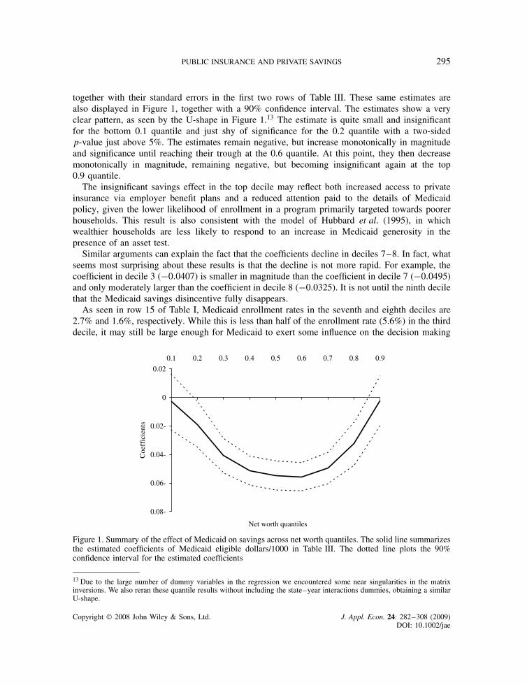
together with their standard errors in the first two rows of Table III. These same estimates arealso displayed in Figure 1, together with a 90% confidence interval. The estimates show a veryclear pattern, as seen by the U-shape in Figure 1.13 The estimate is quite small and insignificantfor the bottom 0.1 quantile and just shy of significance for the 0.2 quantile with a two-sidedp-value just above 5%. The estimates remain negative, but increase monotonically in magnitudeand significance until reaching their trough at the 0.6 quantile. At this point, they then decreasemonotonically in magnitude, remaining negative, but becoming insignificant again at the top0.9 quantile.
The insignificant savings effect in the top decile may reflect both increased access to privateinsurance via employer benefit plans and a reduced attention paid to the details of Medicaidpolicy, given the lower likelihood of enrollment in a program primarily targeted towards poorerhouseholds. This result is also consistent with the model of Hubbard et al. (1995), in whichwealthier households are less likely to respond to an increase in Medicaid generosity in thepresence of an asset test.
Similar arguments can explain the fact that the coefficients decline in deciles 7–8. In fact, whatseems most surprising about these results is that the decline is not more rapid. For example, thecoefficient in decile 3 (�0.0407) is smaller in magnitude than the coefficient in decile 7 (�0.0495)and only moderately larger than the coefficient in decile 8 (�0.0325). It is not until the ninth decilethat the Medicaid savings disincentive fully disappears.
As seen in row 15 of Table I, Medicaid enrollment rates in the seventh and eighth deciles are2.7% and 1.6%, respectively. While this is less than half of the enrollment rate (5.6%) in the thirddecile, it may still be large enough for Medicaid to exert some influence on the decision making
0.08-
0.06-
0.04-
0.02-
0
0.02
0.1 0.2 0.3 0.4 0.5 0.6 0.7 0.8 0.9
Net worth quantiles
Coe
ffic
ient
s
Figure 1. Summary of the effect of Medicaid on savings across net worth quantiles. The solid line summarizesthe estimated coefficients of Medicaid eligible dollars/1000 in Table III. The dotted line plots the 90%confidence interval for the estimated coefficients
13 Due to the large number of dummy variables in the regression we encountered some near singularities in the matrixinversions. We also reran these quantile results without including the state–year interactions dummies, obtaining a similarU-shape.
Copyright 2008 John Wiley & Sons, Ltd. J. Appl. Econ. 24: 282–308 (2009)DOI: 10.1002/jae
296 A. MAYNARD AND J. QIU
of households in these deciles. Moreover, the potential availability of Medicaid in future badstates, such as unemployment spells, may influence savings behavior in households not currentlyenrolled or eligible for Medicaid. As seen in row 14 of Table I, the percentage of householdswith a positive probability of future Medicaid eligibility is considerably higher than the currentenrollment: 0.18 and 0.16 in deciles 7 and 8, respectively. To the extent that moderately wealthyhouseholds view inter-vivos transfers as a potential mechanism for circumventing future Medicaideligibility requirements, this may further enhance the role of Medicaid policy in their savingsdecisions. Finally, if health is a normal good then wealthier households would demand morehealth services14 and might therefore keep a larger buffer stock available as precautionary savingsin the absence of Medicaid. Thus, it is not inconceivable that Medicaid would impact the savingsdecisions of these households.
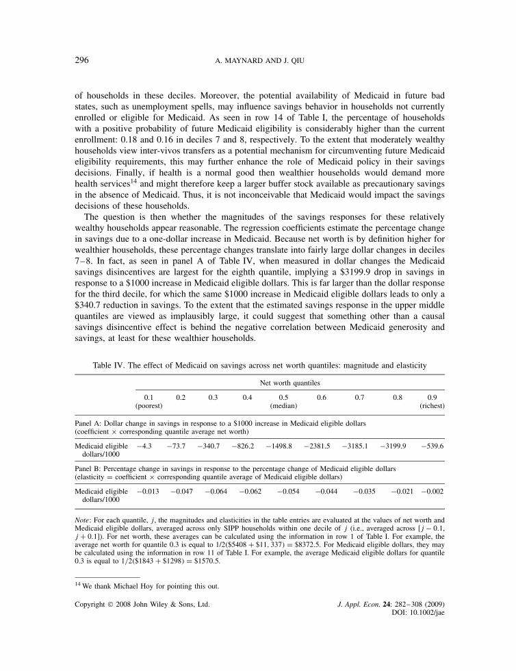
The question is then whether the magnitudes of the savings responses for these relativelywealthy households appear reasonable. The regression coefficients estimate the percentage changein savings due to a one-dollar increase in Medicaid. Because net worth is by definition higher forwealthier households, these percentage changes translate into fairly large dollar changes in deciles7–8. In fact, as seen in panel A of Table IV, when measured in dollar changes the Medicaidsavings disincentives are largest for the eighth quantile, implying a $3199.9 drop in savings inresponse to a $1000 increase in Medicaid eligible dollars. This is far larger than the dollar responsefor the third decile, for which the same $1000 increase in Medicaid eligible dollars leads to only a$340.7 reduction in savings. To the extent that the estimated savings response in the upper middlequantiles are viewed as implausibly large, it could suggest that something other than a causalsavings disincentive effect is behind the negative correlation between Medicaid generosity andsavings, at least for these wealthier households.
Table IV. The effect of Medicaid on savings across net worth quantiles: magnitude and elasticity
Net worth quantiles
0.1(poorest)
0.2 0.3 0.4 0.5(median)
0.6 0.7 0.8 0.9(richest)
Panel A: Dollar change in savings in response to a $1000 increase in Medicaid eligible dollars(coefficient ð corresponding quantile average net worth)
Medicaid eligibledollars/1000
�4.3 �73.7 �340.7 �826.2 �1498.8 �2381.5 �3185.1 �3199.9 �539.6
Panel B: Percentage change in savings in response to the percentage change of Medicaid eligible dollars(elasticity D coefficient ð corresponding quantile average of Medicaid eligible dollars)
Medicaid eligibledollars/1000
�0.013 �0.047 �0.064 �0.062 �0.054 �0.044 �0.035 �0.021 �0.002
Note: For each quantile, j, the magnitudes and elasticities in the table entries are evaluated at the values of net worth andMedicaid eligible dollars, averaged across only SIPP households within one decile of j (i.e., averaged across [j � 0.1,j C 0.1]). For net worth, these averages can be calculated using the information in row 1 of Table I. For example, theaverage net worth for quantile 0.3 is equal to 1/2�$5408 C $11, 337� D $8372.5. For Medicaid eligible dollars, they maybe calculated using the information in row 11 of Table I. For example, the average Medicaid eligible dollars for quantile0.3 is equal to 1/2�$1843 C $1298� D $1570.5.
14 We thank Michael Hoy for pointing this out.
Copyright 2008 John Wiley & Sons, Ltd. J. Appl. Econ. 24: 282–308 (2009)DOI: 10.1002/jae

PUBLIC INSURANCE AND PRIVATE SAVINGS 297
On the other hand, this comparison corresponds to a policy experiment in which the expectedvalue of Medicaid is expanded as much for wealthy households as for poor households. However,recall that the expected value of Medicaid (MED) equals the probability of eligibility times thevalue of benefits to eligible households. Given that the eligibility probabilities are much lower forwealthier households, such a policy would require a greater increase in the dollar value of benefitsto eligible wealthy households than to eligible poor households. An alternative policy experimentwould be one in which the value of Medicaid is expanded proportionally for each quantile ratherthan by an equal fixed dollar amount for the whole population. This experiment could have verydifferent implications because a $1000 increase in the expected value of Medicaid corresponds toa 133.5% increase in the average expected value for households in decile 7, but only a 54.3%increase in decile 3. Therefore, we next examine the percentage change in savings in response to aone-percentage change in the average value of Medicaid eligible dollars in each quantile. Panel Bof Table IV displays these elasticities, which show a similar U-shape as the coefficient estimates.However, the elasticities for deciles 7–8 are considerably lower than those for deciles 3–4.15
Most interesting is the effect of Medicaid on the lower net worth quantiles to whom Medicaidis generally targeted. For these households, the value of Medicaid is quite large relative tonet worth. Thus, one might have expected a more pronounced savings response to Medicaidin the bottom quantiles, whereas they in fact respond much less. As shown in Table III, thecoefficients on Medicaid eligible dollars for the bottom two deciles are �0.0031 (insignificant) and�0.0190 (nearly significant), respectively. The effect becomes strongly significant and increasesin magnitude to �0.0407 and �0.0513, respectively, for the third and fourth deciles.
Although this result may seem surprising given the importance of Medicaid to poorer households,two plausible explanations nevertheless present themselves. The first is that households in thelower quantile have little to no precautionary savings to draw down in response to an expansionin Medicaid eligibility. Average net worth excluding home and car equity, shown in Table I,are already negative for the bottom two deciles. Likewise, given their credit constraints, thesehouseholds may also have little capacity to borrow further. Presumably, in the absence of wealthand borrowing constraints, they would respond to the reduction of future medical expenditureuncertainties associated with increased Medicaid generosity by reducing their savings or increasingtheir borrowing. However, this precautionary saving channel may be blocked on account of lowwealth levels and borrowing constraints. As we explore below, a second possible explanation isthat the asset-testing channel may also become less important in the marginal savings decisionsof the poorest households.
3.3. Asset Testing across Quantiles
By including the interaction between Medicaid eligible dollars and asset testing in their regres-sion,16 Gruber and Yelowitz (1999) find that the average savings disincentive effect of Medicaid
15 Because the regressor, MED, enters in levels, the formula for the elasticity is given by ˛��� MED, where ˛��� is thequantile coefficient on MED and thus depends on the value of MED at which it is evaluated. For the regression it iscommon to evaluate this at the sample average, but since average values of MED differ substantially across low and highnet worth quantiles this would likely be misleading for quantiles other than the median. Instead, for each quantile, say�, we estimate the average value of MED across only those households whose net worth is within one decile of � (i.e.,within � š 0.1).16 Note that the state, year, and state–year interaction dummy variables, which absorb the asset test dummy variable,control for the independent effect of the asset test on net worth.
Copyright 2008 John Wiley & Sons, Ltd. J. Appl. Econ. 24: 282–308 (2009)DOI: 10.1002/jae
298 A. MAYNARD AND J. QIU
is doubled in the presence of an asset test. (Their regression results are reproduced in the secondcolumn of Table V.) In particular, households appear to substantially spend down their wealth togain Medicaid eligibility in the presence of an asset test, once other binding Medicaid eligibilityrequirements, such as income tests or demographic restrictions, are removed. This confirmed oneof the main predictions of Hubbard et al. (1995). A second important prediction of Hubbard et al.(1995), so far unaddressed, is that the effect of the asset test should differ substantially acrosshouseholds of different means. In this section, we investigate the differential impact of Medicaidasset tests across net worth quantiles through the inclusion of the asset test interaction in theinstrumental quantile regression.
While the average impact of Medicaid is found to be particularly strong in the presence ofan asset test, this tells us little about the variation of this effect across quantiles. One mightconjecture that the extent to which a household’s saving decision is affected by the assettest should depend, in part, on the level of its net worth relative to the asset test ceiling. Inparticular, it may depend on whether the household’s wealth is below or above the asset ceilingand, if above, then by how much. The stylized model in Hubbard et al. (1995) implies thathouseholds with initial wealth not too far above asset testing ceilings will react strongly tothe asset test, whereas very wealthy households should not react at all, since they are willingto forgo Medicaid benefits in order to avoid the asset test. In addition, we have argued abovethat households whose initial wealth lies below the asset test ceiling may also be less affectedby asset test interactions, since they require no further asset reductions in order to qualify forMedicaid.
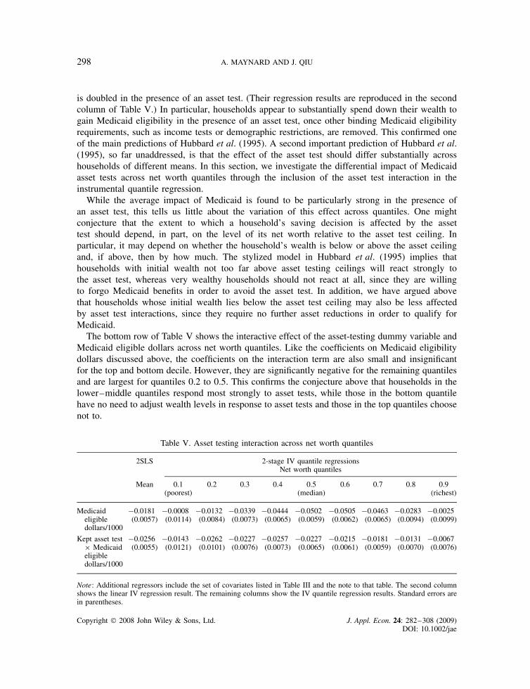
The bottom row of Table V shows the interactive effect of the asset-testing dummy variable andMedicaid eligible dollars across net worth quantiles. Like the coefficients on Medicaid eligibilitydollars discussed above, the coefficients on the interaction term are also small and insignificantfor the top and bottom decile. However, they are significantly negative for the remaining quantilesand are largest for quantiles 0.2 to 0.5. This confirms the conjecture above that households in thelower–middle quantiles respond most strongly to asset tests, while those in the bottom quantilehave no need to adjust wealth levels in response to asset tests and those in the top quantiles choosenot to.
Table V. Asset testing interaction across net worth quantiles
2SLS 2-stage IV quantile regressionsNet worth quantiles
Mean 0.1(poorest)
0.2 0.3 0.4 0.5(median)
0.6 0.7 0.8 0.9(richest)
Medicaid �0.0181 �0.0008 �0.0132 �0.0339 �0.0444 �0.0502 �0.0505 �0.0463 �0.0283 �0.0025eligibledollars/1000
(0.0057) (0.0114) (0.0084) (0.0073) (0.0065) (0.0059) (0.0062) (0.0065) (0.0094) (0.0099)
Kept asset test �0.0256 �0.0143 �0.0262 �0.0227 �0.0257 �0.0227 �0.0215 �0.0181 �0.0131 �0.0067ð Medicaideligibledollars/1000
(0.0055) (0.0121) (0.0101) (0.0076) (0.0073) (0.0065) (0.0061) (0.0059) (0.0070) (0.0076)
Note: Additional regressors include the set of covariates listed in Table III and the note to that table. The second columnshows the linear IV regression result. The remaining columns show the IV quantile regression results. Standard errors arein parentheses.
Copyright 2008 John Wiley & Sons, Ltd. J. Appl. Econ. 24: 282–308 (2009)DOI: 10.1002/jae

PUBLIC INSURANCE AND PRIVATE SAVINGS 299
The table also shows the coefficients on Medicaid eligible dollars after controlling for theinteraction between Medicaid eligible dollars and the asset test (top row). These coefficientsmay now be interpreted as showing the influence of Medicaid eligible dollars on the quantilesof net worth in the absence of the asset test. In other words, they are likely to capture thepure wealth or precautionary savings effects. It is interesting to compare these estimates to theequivalent coefficients on Medicaid eligible dollars in Table III (top row), in which we do notcontrol for the interaction with asset testing. This comparison is presented in Figure 2. The heightof the dark bars on the left shows the coefficients on Medicaid eligible dollars from Table III,where we do not control for asset testing. The gray bars in the middle show the coefficients onMedicaid eligible dollars from Table V after controlling for the asset-testing interaction. Finally,the white bars on the right show the value of the coefficient on the interaction term describedabove.
Inspection of Figure 2 reveals that, after controlling for the asset test interactions in Table V,the coefficients on Medicaid eligible dollars are uniformly reduced across quantiles relative to theoriginal estimates in Table III. This confirms that asset testing interactions can explain part ofthe net worth reductions associated with Medicaid. This appears to be true across all net worthdeciles.
Therefore, it is clear that asset testing plays an important role in the savings decision. On theother hand, although the coefficients on Medicaid eligible dollars in Table V are somewhat smallerin magnitude than those shown in Table III, they nonetheless remain significant for all but thetop decile and the bottom two deciles. In fact, for most of the middle deciles, they remain highlysignificant. Thus, as expected, asset testing explains part, but not all, of the negative effect ofMedicaid on net worth.
Likewise, after controlling for asset testing interactions, the coefficients on Medicaid eligibledollars in Table V, shown by the middle bars of Figure 2, show only a somewhat attenuated
-0.07
-0.05
-0.03
-0.01
0.01
0.1 0.2 0.3 0.4 0.5 0.6 0.7 0.8 0.9
Net worth quantiles
Coe
ffic
ient
s
Figure 2. Summary of the results in Tables III and V. The left (dark), middle (gray) and right (white)columns represent the estimated coefficients on Medicaid eligible dollars/1000 in Table III, Medicaid eligibledollars/1000 in Table V and Kept asset testing ð Medicaid eligible dollars/1000 in Table V, respectively.
Copyright 2008 John Wiley & Sons, Ltd. J. Appl. Econ. 24: 282–308 (2009)DOI: 10.1002/jae

300 A. MAYNARD AND J. QIU
version of the original U-shape found in the coefficients in Table III (the left bars in Figure 2).Even after accounting for asset testing, we still find a much stronger effect of Medicaid eligibledollars on the middle quantiles than we do on the top and bottom ends of the distribution. In otherwords, asset testing is again just part of the story. Differential responses to asset testing explainonly some of the differences across quantiles. The remaining differences must be explained byother channels. As discussed above, for the top decile this may simply reflect the fact that Medicaidplays a much smaller relative role in household finances. For the bottom quantiles, we have arguedabove that low existing precautionary savings and constraints on borrowing may limit the normalprecautionary savings effect.
3.4. Results Including Households with Negative Net Worth
In the results presented above, we excluded households with non-positive net worth. This allowedus to employ a log transformation of net worth, thereby providing a convenient interpretation ofthe coefficients in terms of percentage changes. It also allowed for a clean comparison to the earlierresults of Gruber and Yelowitz (1999), whose regression results are estimated using householdswith positive net worth. Nevertheless, in order both to ensure robustness to potential sampleselection concerns17 and also to estimate the effects of Medicaid on the very poorest households,it is necessary to include households with zero or negative net worth. As these households arerelatively likely to qualify for Medicaid and also have the least savings, it may be of interest toconsider this sub-population when analyzing the effect of Medicaid on savings.
We now expand our sample to include the households with zero or negative net worth in additionto the positive net-worth households employed above. This yields a total of 52,706 households,of which 7043 (or 13.36%) report zero net worth and 5221 (or 9.91%) report negative net worth.
Because the log transformation is defined only for positive values, we may no longer employlog net worth as our dependent variable. This issue arises often when working with wealth data.As a solution to this problem, Burbidge et al. (1988) and Pence (2006) suggest transforming networth by the inverse hyperbolic sine transformation
g�yt, �� D log��yt C ��2y2t C 1�1/2�/� D sinh�1��yt� �10�
which admits non-positive values of yt, in place of the more standard log transformation. Thistransformation of net worth has been employed in recent work by Cobb-Clark and Hildebrand(2006) using a value of � D 1, in which case it simplifies to
g�yt, 1� D log�yt C �y2t C 1�1/2� D sinh�1�yt� �11�
In the results discussed below, we also employ the specialized version of the inverse hyperbolicsine transformation given in (11).18
17 Gruber and Yelowitz (1999) also provide probit results on the probability of a household’s having positive net worthand use these results to convincingly argue that sample selection bias could not be large enough to undo their main results.18 The transformation in (10) is linear near the origin but approximates a vertically shifted log-function for large positiveyt values. The parameter � governs both the speed of this transition and the size of the shift. Using � D 1 we closelyapproximate (by less than a $1.0 difference) our previous log specification for positive net worth values as small as $100.By contrast, employing a value of � near zero approximates the regression in levels for all but very large values of jyj.
Copyright 2008 John Wiley & Sons, Ltd. J. Appl. Econ. 24: 282–308 (2009)DOI: 10.1002/jae

PUBLIC INSURANCE AND PRIVATE SAVINGS 301
Table VI shows the instrumental quantile regression results including households with positive,negative, and zero net worth. The dependent variable in both panels is the inverse hyperbolic sinetransformation of net worth. Panel A, which shows quantile coefficients describing the effect ofMedicaid on net-worth, employs the same regressor, instrument, and control variates as Table III.Likewise, panel B, which includes also the asset test dummy variable, includes the same regressors,instruments, and control variates as in Table V.
With the exception of the first two deciles, for which net worth (y) is zero, simple cal-culations show that the coefficient estimates in panel A of Table VI closely approximate the
quantity ∂y/∂MEDjyj that corresponds to the interpretation of the coefficient on MED in the pre-
vious log-level specification employed in Table III.19 This is expected since the transformationin (11) closely resembles the log transformation for all but the poorest positive net worthhouseholds (see footnote 18). Thus, the coefficients in Table VI using the inverse hyperbolictransform have (approximately) the same interpretation as those using the log specification inTable III.
On the other hand, due to the inclusion of non-positive net worth households, the � quantilein Table VI corresponds to a lower value of net worth than the same � quantile in Table III.Therefore, one cannot meaningfully compare the magnitudes of the coefficients across thesetables. Nevertheless we may still compare the overall shape and pattern of the quantile coef-ficients. In panel A, we again observe a U-shaped pattern to the quantile coefficients. Thisconfirms our earlier finding that the savings effect of Medicaid is strongest in the middle networth quantiles. However, because we no longer truncate the non-positive net worth house-holds, this U-shape is shifted somewhat to the right. For example, using this full sample,the bottom two quantile coefficients are insignificant, whereas in Table III only the bottomcoefficient turned up insignificant. Thus, we find no discernible effect of Medicaid on thesavings on the bottom 20% of households, when including households with non-positive networth.
The quantile coefficients in Table VI, panel B, also show a pattern similar to those in Table V.The top row shows the effect on the quantiles of net worth in the absence of an asset test,while the third row shows the quantile coefficients on the asset-test/Medicaid interaction term.Standard errors are given in parentheses below the estimates. The negative savings effect ofthe Medicaid/asset test interaction term is again strongest for the lower–middle net worthquantiles. As before, this effect dissipates in the top quantiles and it now disappears altogetherfor the bottom two deciles. In fact, somewhat surprisingly, these two coefficients have a positivesign.
To investigate the robustness of our choice, in results available upon request, we have also rerun our results using valuesof � ranging between 0.1 and 10, obtaining similar overall U-shaped patterns. Burbidge et al. (1988) and Pence (2006)develop methods for selecting � in mean and median regression, respectively, but we are not aware of existing selectionmethods for general quantile or IV regression.19 In fact, these approximations are accurate out to at least seven digits. The corresponding comparisons for the coefficientsin panel B apply up to a similar margin of approximation error. For large jyj, this close approximation can be understood
by the relation ∂y/∂MEDjyj D ˛����1/jyj�(
1∂g�y, 1�/∂y
)³ ˛���, where ∂g�y, 1�/∂y D �y2 C 1�1/2 C y
y�y2 C 1�1/2 C �y2 C 1�. For deciles
1 and 2 y D 0, so that ∂y/∂MEDjyj is not well defined.
Copyright 2008 John Wiley & Sons, Ltd. J. Appl. Econ. 24: 282–308 (2009)DOI: 10.1002/jae

302 A. MAYNARD AND J. QIU
Tabl
eV
I.R
esul
tsin
clud
ing
hous
ehol
dsw
ith
non-
posi
tive
net
wor
thqu
anti
les
2SL
S2-
stag
eIV
quan
tile
regr
essi
ons
Net
-wor
thqu
antil
es
Pane
lA
:T
heef
fect
ofM
edic
aid
onsa
ving
sac
ross
net
wor
thqu
antil
es
Mea
n0.
1(p
oore
st)
0.2
0.3
0.4
0.5
(med
ian)
0.6
0.7
0.8
0.9
(ric
hest
)
Med
icai
del
igib
ledo
llars
/100
0�0
.053
7�0
.006
80.
0013
�0.0
690
�0.0
900
�0.1
161
�0.1
274
�0.1
056
�0.0
786
�0.0
533
(0.0
135)
(0.0
606)
(0.0
245)
(0.0
132)
(0.0
109)
(0.0
081)
(0.0
077)
(0.0
097)
(0.0
082)
(0.0
083)
Pane
lB
:A
sset
test
ing
inte
ract
ion
acro
ssne
tw
orth
quan
tiles
Mea
n0.
1(p
oore
st)
0.2
0.3
0.4
0.5
(med
ian)
0.6
0.7
0.8
0.9
(ric
hest
)
Med
icai
del
igib
ledo
llars
/100
0�0
.050
6�0
.032
3�0
.017
6�0
.066
2�0
.079
8�0
.106
9�0
.115
6�0
.093
2�0
.070
4�0
.051
1(0
.014
1)(0
.055
8)(0
.027
9)(0
.013
5)(0
.010
8)(0
.008
7)(0
.009
0)(0
.010
8)(0
.007
9)(0
.008
6)
Kep
tas
set
test
ðM
edic
aid
�0.0
145
0.12
560.
0434
�0.0
292
�0.0
537
�0.0
455
�0.0
381
�0.0
372
�0.0
273
�0.0
183
elig
ible
dolla
rs/1
000
(0.0
128)
(0.0
379)
(0.0
225)
(0.0
129)
(0.0
095)
(0.0
079)
(0.0
076)
(0.0
073)
(0.0
062)
(0.0
059)
Not
e:T
hesa
mpl
ein
clud
esal
l(5
2,70
6)ho
useh
olds
with
posi
tive,
zero
and
nega
tive
net
wor
thin
SIPP
.The
depe
nden
tva
riab
leis
the
hype
rbol
icsi
gntr
ansf
orm
atio
nof
net
wor
th.
Add
ition
alre
gres
sors
incl
ude
the
set
ofco
vari
ates
liste
din
Tabl
eII
Ian
dth
eno
teto
that
tabl
e.T
hese
cond
colu
mn
show
sth
elin
ear
IVre
gres
sion
resu
lts.
The
rem
aini
ngco
lum
nssh
owth
eIV
quan
tile
regr
essi
onre
sults
.St
anda
rder
rors
are
inpa
rent
hese
s.
Copyright 2008 John Wiley & Sons, Ltd. J. Appl. Econ. 24: 282–308 (2009)DOI: 10.1002/jae

PUBLIC INSURANCE AND PRIVATE SAVINGS 303
3.5. The Interaction between Labor Income, Medicaid, and Asset Testing
Incorporating information on labor income provides two important robustness checks. First,following Gruber and Yelowitz (1999), our baseline specification excluded labor income under theassumption that labor income is orthogonal to the instrument (SIMMED). However, it is possiblethat this assumption could be violated in practice. For example, it would be unlikely to hold ifincome varies across household sizes. Labor income can also be used to assess the sensitivity ofour qualitative conclusions to the implicit use of net worth as the indicator of affluence. In the workpresented above, we examined the effect of Medicaid on savings across households with differentwealth levels. However, net worth is just one measure of a family’s affluence (or poverty). Somefamilies may have high income, but low or negative net worth. An example would be a head ofhousehold who recently graduated from college with a good job but large student loans. Therefore,we also consider the robustness of our findings when affluence/poverty is defined in terms of laborincome instead of wealth holdings. In other words, we consider the savings disincentive effectsof Medicaid as a function of household income rather than household wealth. In order to mitigateendogeneity between net worth and income, we focus exclusively on labor income.
In column 1 of Table VII, we re-estimate the mean results for households with positive networth shown in column 1 of Table III with the log of family labor income added as an additionalcontrol variate. The results confirm that labor income is important in explaining net worth, butits inclusion does not much change the regression coefficient on Medicaid eligible dollars.20 Incolumn 2, we estimate the mean effect for the households with positive and non-positive net worth,again controlling for labor income. For this population, the mean effect becomes insignificant,suggesting that the mean effect differs depending on the population under consideration. Thisis consistent with our earlier finding that savings disincentives are weaker and insignificant forpoorer households, many of whom are excluded from the regression including only householdswith positive net worth.
In order to explore these results further and also to assess the robustness of our findings whenaffluence is redefined in terms of income rather than wealth, we next consider the savings effectof Medicaid as a function of labor income. Since net worth is the dependent variable, the quantileregression is the appropriate approach when considering the savings effect of Medicaid as afunction of net worth. However, the quantile regression is no longer appropriate when consideringthe savings effect of Medicaid as a function of labor income, since labor income is not thedependent variable and must instead be treated as a regressor. Therefore, in column 3 of Table VII,we instead interact Medicaid with dummy variables corresponding to the five quintile rangesranges of labor income.21 The last four of these dummy variables are denoted by Labor incomequintile j, j D 2, 3 . . . 5 and shown in the bottom four rows of column 1.22 The five interactionterms, denoted by Medicaid eligible dollars/1,000 ð Labor income quintile j, j D 1, 2, . . . , 5, areshown in rows 3–7 of Table VII. We instrument the Medicaid interaction term variables in rows3–7 using the interaction of the labor quintile dummy variables with SIMMED, the instrumentemployed previously for Medicaid eligible dollars. We employ the same sample, dependent variable
20 In results available upon request, we also found IV quantile results similar to those in Table III when controlling forlabor income.21 Because approximately the bottom 20% of households in our sample have no labor income, we break labor incomeinto quintiles rather than deciles.22 Both the first labor income dummy variable and Medicaid eligible dollars themselves are excluded in order to avoidthe dummy variable trap.
Copyright 2008 John Wiley & Sons, Ltd. J. Appl. Econ. 24: 282–308 (2009)DOI: 10.1002/jae
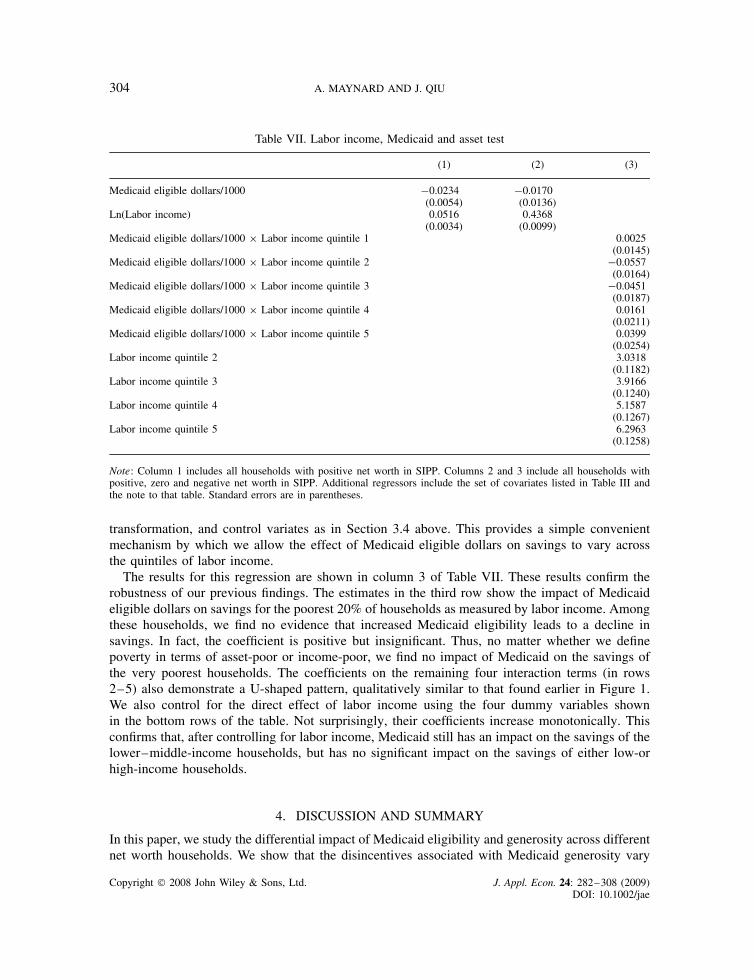
304 A. MAYNARD AND J. QIU
Table VII. Labor income, Medicaid and asset test
(1) (2) (3)
Medicaid eligible dollars/1000 �0.0234 �0.0170(0.0054) (0.0136)
Ln(Labor income) 0.0516 0.4368(0.0034) (0.0099)
Medicaid eligible dollars/1000 ð Labor income quintile 1 0.0025(0.0145)
Medicaid eligible dollars/1000 ð Labor income quintile 2 �0.0557(0.0164)
Medicaid eligible dollars/1000 ð Labor income quintile 3 �0.0451(0.0187)
Medicaid eligible dollars/1000 ð Labor income quintile 4 0.0161(0.0211)
Medicaid eligible dollars/1000 ð Labor income quintile 5 0.0399(0.0254)
Labor income quintile 2 3.0318(0.1182)
Labor income quintile 3 3.9166(0.1240)
Labor income quintile 4 5.1587(0.1267)
Labor income quintile 5 6.2963(0.1258)
Note: Column 1 includes all households with positive net worth in SIPP. Columns 2 and 3 include all households withpositive, zero and negative net worth in SIPP. Additional regressors include the set of covariates listed in Table III andthe note to that table. Standard errors are in parentheses.
transformation, and control variates as in Section 3.4 above. This provides a simple convenientmechanism by which we allow the effect of Medicaid eligible dollars on savings to vary acrossthe quintiles of labor income.
The results for this regression are shown in column 3 of Table VII. These results confirm therobustness of our previous findings. The estimates in the third row show the impact of Medicaideligible dollars on savings for the poorest 20% of households as measured by labor income. Amongthese households, we find no evidence that increased Medicaid eligibility leads to a decline insavings. In fact, the coefficient is positive but insignificant. Thus, no matter whether we definepoverty in terms of asset-poor or income-poor, we find no impact of Medicaid on the savings ofthe very poorest households. The coefficients on the remaining four interaction terms (in rows2–5) also demonstrate a U-shaped pattern, qualitatively similar to that found earlier in Figure 1.We also control for the direct effect of labor income using the four dummy variables shownin the bottom rows of the table. Not surprisingly, their coefficients increase monotonically. Thisconfirms that, after controlling for labor income, Medicaid still has an impact on the savings of thelower–middle-income households, but has no significant impact on the savings of either low-orhigh-income households.
4. DISCUSSION AND SUMMARY
In this paper, we study the differential impact of Medicaid eligibility and generosity across differentnet worth households. We show that the disincentives associated with Medicaid generosity vary
Copyright 2008 John Wiley & Sons, Ltd. J. Appl. Econ. 24: 282–308 (2009)DOI: 10.1002/jae

PUBLIC INSURANCE AND PRIVATE SAVINGS 305
considerably across household net worth quantiles. In fact, we uncover a clear U-shaped patternacross the quantile coefficients, with the disincentive effect peaking near the middle of the networth distribution, but becoming small and insignificant at both its top and bottom end.
Our results have several important implications. In particular, there is no evidence that Medicaidexpansions crowd out the savings of the very poorest households, whereas crowd-out may besubstantial for moderately poor households. Surprisingly, the crowd-out is also large for moderatelywealthy households (deciles 7–8), especially when responses are measured in dollar magnitudes.The crowd-out effect is generally heightened in the presence of an asset test, particularly for thelower–middle quantiles of the asset and income distributions. Yet, even with an asset test in place,there is still no evidence of savings crowd-out for the bottom quantiles.
This has interesting economic implications. We find that Medicaid generosity has little savingseffect for the wealthiest households (decile 9), but quite a strong effect on households in themiddle quantiles. Moreover, in the presence of an asset test, the effect appears to be strongest forthose households whose asset levels are not much above the asset test ceiling. This is generallysupportive of the central theoretical mechanism at work in Hubbard et al. (1995), in which theutility cost of the savings adjustment required to meet the asset test is moderate for poor householdsbut becomes prohibitive for wealthier households.
On the other hand, we find no evidence of Medicaid induced savings disincentives for householdsin the bottom quantiles of either the income or wealth distributions. This is also consistent with thefindings of Hurst and Ziliak (2006), who find no evidence of asset-test based savings disincentivesfor female-headed households with children, a demographic whose wealth and earnings areconcentrated in the lower quantiles. Several potential explanations for the lack of savings responseby poor households present themselves. First, since many of these households have virtually noprecautionary savings to spend down and little room to borrow on account of their low income,they may not be able to further reduce their precautionary savings in response to a Medicaidexpansion. Likewise, these same households have too few assets to be affected by the assettest limits. Secondly, the poorest households are likely to be eligible for other public insuranceprograms and may therefore be less responsive to changes in Medicaid coverage. For example, ahousehold might not increase its savings in response to the removal of the Medicaid asset test ifthey still need to satisfy asset tests to qualify for other government programs.23 This suggests that itmay be important to study the combined impact of public insurance programs on poor households.It may also be possible that some of these households are myopic (Feldstein, 1987), and thus donot respond to Medicaid incentives. Alternatively, given low incomes, they may envision littleprospect of accumulating precautionary savings substantial enough to be useful in the event oflarge discrete medical costs. More work may be required to fully understand their lack of savings.
Finally, we acknowledge some caveats associated with this reduced form approach.24 From theperspective of a life cycle model, what we attempt to capture is essentially the impact of solving themodel with and without Medicaid policy, holding all other aspects constant. Despite the carefullydeveloped instrument and the many control variates included in the empirical specifications, thereare still some reasons to suspect that the estimates from our reduced-form approach may differ incertain respects from the structural effects that are of ultimate interest.
23 Similarly, French and Jones (2004, see section 4.3 of their extended version) find an inverted U-shape to the value thathouseholds would be willing to pay for health insurance. They attribute this to the fact that the poorest households arealready protected by an implicit consumption floor.24 We thank the co-editor, John Rust, for several very thoughtful comments on these issues.
Copyright 2008 John Wiley & Sons, Ltd. J. Appl. Econ. 24: 282–308 (2009)DOI: 10.1002/jae

306 A. MAYNARD AND J. QIU
First, the identification strategy treats policy changes as if they were exogenous experimentsrather than outcomes of a policy process, which, while exogenous to individual level householdnet worth, may respond to larger trends in wealth or other household characteristics. For example,increases in average wealth may help accommodate more generous public insurance via anexpanded tax base. Likewise, trends in household composition, such as the proportion of single-headed households, may alter the political constituencies that support Medicaid. As discussed inSection 2.2, to some extent this endogeneity may be partially (but only partially) mitigated, via theinclusion of year–state interaction dummy variables that partial out the policy induced variationbetween state–year cells. The identification relies rather on the within state–year variation inhousehold responses to these policy changes that arise due to differences in the quasi-exogenoushousehold characteristics, such as family member ages, used in the instrumental variable.
A second potential concern is that we do not control for the value of other public insuranceprograms, such as Supplementary Security Income (SSI) and Aid to Families with DependentChildren (AFDC). This may bias the results in either direction by confounding changes in thegenerosity of other social insurance programs with those of Medicaid. In addition, complicatedinteractions between the asset tests of various programs could exist. For example, householdsenrolled in multiple programs may not increase their savings until all relevant asset tests are lifted.This issue could, in principle, be partially addressed in a reduced-form context by developinghousehold present expected value measures, similar to the Medicaid eligible dollars measureof Currie and Gruber (1996a,b), for programs such as SSI and AFDC. While this may be aninteresting line of future research, without the aid of a structural model, it is not clear whether thesimple inclusion of these measures as control variates would be sufficient to capture the complexinteractions between government programs.
Certain higher-level general equilibrium effects that might be expected from large changes inMedicaid policy may also be missed by our analysis. For example, in the absence of Medicaid, theremight be greater incentives for low-wage employers to provide medical insurance, or insurers mighttailor new private health insurance plans to low-income households. Likewise, the composition ofthe health care industry and thus health costs might also be affected by the removal of a largegovernment purchaser.
In future research, it might be interesting to further distinguish between the different channelsby which Medicaid impacts savings. For example, public insurance programs, particularly whencoupled with a means test, may also lead to reductions in labor income, which may in turn reducesavings. The savings disincentives which we estimate combine this indirect channel with the directimpact of Medicaid, whereas it might be useful in future work to disentangle the two. It wouldalso be interesting to distinguish between true reductions in savings and inter-vivos transfers.
ACKNOWLEDGEMENTS
We are grateful to Jonathan Gruber and Aaron Yelowitz for generously providing us with theirdata. We also thank Victor Chernozhukov and Christian Hansen for use of their instrumentalquantile regression code. This paper has benefited substantially from comments by John Rustand two anonymous referees. We also thank Varouj Aivazian, Michael Baker, Stacey Chen,Chuan Goh, Vincent Hildebrand, Kim Huynh, Michael Hoy, John Bailey Jones, Lonnie Magee,Robert McMillan, Christine Neill, Karen Pence, Eduardo Pontual Ribeiro, Jeff Racine, AloysiusSiow (discussant), Michael Smart, seminar participants at SUNY Albany and McMaster, and
Copyright 2008 John Wiley & Sons, Ltd. J. Appl. Econ. 24: 282–308 (2009)DOI: 10.1002/jae

PUBLIC INSURANCE AND PRIVATE SAVINGS 307
conference participants at the 2005 Canadian Economic Association Meetings and the 2006Midwest Econometrics Group Meeting, for useful comments. The authors acknowledge financialsupport from the Social Science and Humanities Research Council of Canada under grant numbers410-2001-1527 (Maynard) and 410-2005-0206 (Qiu). We take full responsibility for any remainingerrors.
REFERENCES
Abadie A, Angrist J, Imbens G. 2002. Instrumental variables estimates of the effect of subsidized trainingon the quantiles of trainee earnings. Econometrica 70: 91–117.
Burbidge JB, Magee L, Robb AL. 1988. Alternative transformations to handle extreme values of thedependent variable. Journal of the American Statistical Association 83: 123–127.
Cagetti M. 2003. Wealth accumulation over the life cycle and precautionary savings. Journal of Businessand Economic Statistics 21: 339–353.
Chen L-A, Portnoy S. 1996. Two-stage regression quantiles and two-stage trimmed least squares estimatorsfor structural equation models. Communications in Statistics: Theory and Methods 25: 1005–1032.
Chernozhukov V, Hansen C. 2004a. The effect of 401(k) participation on the wealth distribution: aninstrumental quantile regression analysis. Review of Economics and Statistics 86: 735–751.
Chernozhukov V, Hansen C. 2004b. Instrumental quantile regression. Mimeo, Department of Economics,MIT. Available: http://www.mit.edu/¾vchern/papers/ch IVQR 2001 rev Oct24 2004.pdf [accessed 21October 2008].
Chernozhukov V, Hansen C. 2005. An IV model of quantile treatment effects. Econometrica 73: 245–262.Chernozhukov V, Hansen C. 2006. Instrumental quantile regression inference for structural and treatment
effect models. Journal of Econometrics 132: 491–525.Chesher A. 2003. Identification in nonseparable models. Econometrica 71: 1405–1441.Chou S-Y, Liu J-T, Hammitt JK. 2003. National health insurance and precautionary savings: evidence from
Taiwan. Journal of Public Economics 87: 1873–1894.Cobb-Clark DA, Hildebrand VA. 2006. The wealth and asset holdings of US-born and foreign-born house-
holds: evidence from SIPP data. Review of Income and Wealth 52: 17–42.Conley TG, Galenson DW. 1994. Quantile regression analysis of censored wealth data. Historical Methods
27: 149–165.Conley TG, Galenson DW. 1998. Nativity and wealth in mid-nineteenth-century cities. Journal of Economic
History 58: 468–493.Currie J, Gruber J. 1996a. Health insurance eligibility, utilization of medical care, and child health. Quarterly
Journal of Economics 111: 431–466.Currie J, Gruber J. 1996b. Saving babies: the efficacy and cost of recent changes in the Medicaid eligibility
of pregnant women. Journal of Political Economy 104: 1263–1296.Curtin RT, Juster FT, Morgan JN. 1989. Survey estimates of wealth: an assessment of quality. In The
Measurement of Savings, Investment, and Wealth, Lipsey RE, Tice HS (ed.). University of Chicago Press(for NBER): Chicago, IL; 473–552.
Feldstein M. 1987. Should social security benefits be means tested? Journal of Political Economy 95:468–484.
French E, Jones JB. 2004. On the distribution and dynamics of health care costs. Journal of AppliedEconometrics 19: 705–722. Extended version available: http://www.albany.edu/¾jbjones/healc15.pdf [2October 2008].
Gruber J, Yelowitz A. 1999. Public health insurance and private savings. Journal of Political Economy 107:1249–1274.
Horowitz JL, Lee S. 2007. Nonparametric instrumental variables estimation of a quantile regression model.Econometrica 75: 1191–1208.
Hubbard RG, Skinner J, Zeldes SP. 1995. Precautionary saving and social insurance. Journal of PoliticalEconomy 103: 360–399.
Copyright 2008 John Wiley & Sons, Ltd. J. Appl. Econ. 24: 282–308 (2009)DOI: 10.1002/jae

308 A. MAYNARD AND J. QIU
Hurd MD, Hoynes H, Chand H. 1998. Household wealth of the elderly under alternative imputationprocedures. In Inquiries in the Economics of Aging, Wise D (ed.). University of Chicago Press: Chicago,IL; 229–257.
Hurst E, Ziliak J. 2006. Do welfare asset limits affect household saving? Evidence from welfare reform.Journal of Human Resources 41: 46–71.
Hurst E, Luoh MC, Stafford F, Gale W. 1998. The wealth dynamics of American families, 1984–94.Brookings Papers on Economic Activity 1998: 267–337.
Kapteyn A, Alessie R, Lusardi A. 2005. Explaining the wealth holdings of different cohorts: productivitygrowth and social security. European Economic Review 49: 1361–1381.
Koenker R, Bassett GS. 1978. Regression quantiles. Econometrica 46: 33–50.Kotlikoff LJ. 1989. Health expenditures and precautionary savings. In What Determines Savings, Kotlikoff LJ
(ed.). MIT Press: Cambridge, MA; 140–162.Ma L, Koenker R. 2006. Quantile regression methods for recursive structural equation models. Journal of
Econometrics 134: 471–506.Palumbo MG. 1999. Uncertain medical expenses and precautionary saving near the end of the life cycle.
Review of Economic Studies 66: 395–421.Pence KM. 2006. The role of wealth transformations: an application to estimating the effect of tax incentives
on saving. Contributions to Economic Analysis and Policy 5: Article 20. Available: http://www.bepress.com/bejeap/contributions/vol5/iss1/art20 [2 October 2008].
Powell JL. 1983. The asymptotic normality of two-stage least absolute deviations estimators. Econometrica51: 1569–1576.
Powers E. 1998. Does means-testing welfare discourage saving? Evidence from a change in AFDC policyin the United States. Journal of Public Economics 68: 33–53.
Sherraden M. 1991. Assets and the Poor: A New American Welfare Policy. ME Sharp: Armank, NY.Starr-McCluer M. 1996. Health insurance and precautionary savings. American Economic Review 86:
285–295.
Copyright 2008 John Wiley & Sons, Ltd. J. Appl. Econ. 24: 282–308 (2009)DOI: 10.1002/jae


![A Guide for Pensioners and their Dependants[1] Guide/a-guide... · 2020. 7. 22. · pension savings are likely to be adversely affected. If you think you may be affected by the new](https://static.fdocuments.us/doc/165x107/5ff897f48fb8ee74ee158e8c/a-guide-for-pensioners-and-their-dependants1-guidea-guide-2020-7-22.jpg)