Public good production in heterogeneous groups:

An experimental analysis on the relation between external return and

information∗

Gerlinde Fellner-Rohling†, Sabine Kroger‡, Erika Seki§

September 9, 2019

Abstract

In this article, we study voluntary contributions of heterogeneous groups to a public good in anexperiment. Members of the same group have either low or high external marginal returns. We varythe level of information about the heterogeneity and about a contributor’s type between groups.While controlling for the net costs of contributions, we find that the level of information determineshow types in heterogeneous groups vary in their contributions. When the type of a contributorcan be identified, types with high returns contribute more, otherwise the effect disappears or evenreverses with low types contributing more than high types. This result provides evidence for theso-called “poisoning-of-the-well” effect and demonstrates how it interacts with the informationstructure of the environment. Without any information about heterogeneity, there is no differencein contributions by types.

JEL classification: C9; H41Keywords: Public goods; Voluntary contribution mechanism; Heterogeneity in marginal per capitareturns; Internal and external return; Information on types and type specific contributions; Poisoning-of-the-well

∗Our special thanks go to Yoshio Iida from Kyoto Sangyo University, who has provided valuable insights and inputssince the inception of this research. We thank Bettina Bartels and Hakan Fink for their research assistance. We aregrateful to seminar participants at the Department of Economics, Technische Universitat Berlin, Osaka University, andparticipants at the Canadian Economics Association Meeting in Ottawa for their insights and discussion. We gratefullyacknowledge financial support by the Max Planck Institute of Economics in Jena, Germany, and the Kyoto SangyoUniversity, Japan, and the FQRSC (127568). Any errors remain our own.†Institute of Economics, Ulm University, Helmholtzstraße 18, 89081 Ulm, Germany‡Laval University, Department of Economics, Pavillon J.A.DeSeve, Quebec, Quebec G1V 0A6 Canada§Graduate School of Economics, Osaka University, 1-7 Machikanayamacho, Toyonaka-shi, Osaka, 560-0043, Japan

1

1 Introduction

Heterogeneity in general affects cooperation in many ways. Team members who contribute to joint

projects differ, for instance, in their talents, skills, and qualifications. In some cases, heterogeneous

abilities are even necessary to achieve a common goal (Papps et al. (2011)) or to be more productive

(Hamilton et al. (2003)). Although members in heterogeneous groups might be motivated to contri-

bute to a joint project because of concerns for social returns (e.g., Andreoni (1988 and 1990)) and

conditional cooperation (e.g., Fischbacher et al. (2003), Gachter (2007)), the channel through which

heterogeneity among group members affects individual contributions to a joint project is not clear, as

the heterogeneity affects not only the returns, but also the costs of cooperation. In a group with hete-

rogeneous abilities,1 normative conflicts may arise as social preferences themselves could be influenced

by the perception of heterogeneity, namely how individuals perceive their ability and that of others.

Role dependent preferences (as documented by Goeree et al. (2002), Gachter and Riedl (2005)

and Bellemare et al. (2008)) can lead to conflicting views on what contribution norm should apply in

heterogeneous groups, as an example of the Bonn orchestra illustrates. In this context, the rehearsal

time before the performance can be interpreted as the net contribution of each musician to the joint

project, the performances in front of the public. This net contribution varies amongst musicians.

Soloists spend less time rehearsing with the whole group compared to violinists while receiving the

same pay, thus earning a higher relative pay per joint rehearsal time. The management of the Bonn

orchestra justified the difference in the relative pay between violinists and soloists with the excellence

of soloists and their vital contribution to the joint project. The management referred to the high

pressure soloists face when performing and refused to adjust the pay according to the rehearsal time.

Violinists disagreed strongly and made a complaint.2 While violinists considered equal remuneration

of each musician’s nominal work hours as fair, management and soloists seemed to favor remuneration

according to the effective contributions to the joint project, the latter accounting for other factors such

as responsibility, stress, etc. This dispute in the Bonn orchestra illustrates that conflicting views on

fair contributions are likely to emerge in groups with heterogeneous abilities and plural values (Konow

(2000), Konow (2003), Cappelen et al. (2007)).

This example fits the standard conflict in public goods experiments, where contributions increase

the public good by more than what each member contributed. Contributions are costly and the

1In this paper, the term “ability” refers to the external return of a contribution. The external return indicates byhow much a group member’s contribution increases the public good. Other scholars have referred to the external returnalso as “productivity” (Tan (2008)) or “capacity” (Kolle (2015)).

2The case was eventually settled with hiring part-time student violinists for some rehearsals to fill in for the overworkedviolinists (Klassik News, March 24, 2004 and Kolner Stadt-Anzeiger, July 16, 2004 ).

2

returns of the joint project are shared equally among all group members, providing incentives to free

ride. This trade-off represents the social dilemma situation. In other words, contributing to the joint

project is socially efficient but not in the interest of the individual member. It becomes a source of

normative conflicts as multiple contribution norms may arise (Kingsley (2016) and Nikiforakis et al.

(2012)). Conflicting norms may even intensify when persons differ in their ability to contribute to the

public good, as in our example. Two factors that influence voluntary contributions, and thus may

exacerbate or mitigate such conflicts, are the efficiency of contributions and information about others

and their behavior.

In this article, we examine the relationship between information and heterogeneous abilities to

increase a public good. Thereby, we bridge two strands of public goods research. The first studies

the effect of returns on contributions, and the second is looking at how information conditions affect

contributions. The challenges we are confronted with in order to understand the effect of ability on the

contribution to public goods are threefold: first, the literature on groups with heterogeneous marginal

per capita returns does not control for the net costs of contributions. A higher marginal return makes

contributions more efficient and might trigger efficiency concerns or altruistic preferences. However, a

high return also decreases the net costs of contributions to the public good rendering contributions more

affordable, a consequence that has been overlooked so far in the literature that studies heterogeneity in

returns from public goods. Second, the literature on internal and external returns focuses exclusively

on homogeneous groups. This literature cannot address how individuals react when group members

differ in their return rates. And third, the literature on returns and the literature that explicitly

studies the effect of information on public goods focuses only on situations where all group members’

return rates are common knowledge. The literature on information in public goods experiments has

studied the effects of reporting individual or aggregate contribution levels, but has not considered

different types of contributors or varied the information about contributions of different types.

Our experimental design improves on these points. We vary the individual ability within groups

while controlling for the costs of contributing. This allows us to exclude lower net contribution costs

as a motive of high ability members to adjust their contributions in a heterogeneous environment.

We systematically change the information scenarios under which persons make their contribution

decisions, which allows us to better study conflicting social norms of contributing to the public good.

Thus, the novel contribution of this study to the literature is twofold. It is the first to isolate the effect

of external returns on contributions from the net costs of contributing in heterogeneous groups. And,

it presents the first analysis on how information on peers’ abilities affects contributions. In brief, this

is to the best of our knowledge the first study to investigate the effect of the ability to increase the

3

public good and the effect of information on cooperation in heterogeneous groups in a systematic way.

Our results can be summarized as follows. We find that in the absence of information about

heterogeneity in the ability to increase the public good, contributions of both ability types are identical.

When heterogeneity is known to be present, but contributions cannot be linked to the contributors’

types, group members with lower external returns tend to contribute more than those with higher

returns. When, additionally, contributions can be linked to the contributors’ types, individuals with

a higher external returns tend to contribute more than those with lower returns. Given our results,

we can attribute the positive relation between marginal per capita return and contributions reported

in the literature at least partly to the external return and conclude that the relation persists even

when controlling for the net costs of contribution. However, the positive relation of contributions and

the external return holds only as long as there is common knowledge about external returns and the

contributor’s type. As soon as both or only one part of information is lacking, this relation breaks

down. Without any information about the existence of heterogeneity, persons with different returns

make the same nominal contributions, i.e., ensure that they have the same contribution costs. When

individuals know about the heterogeneity, but cannot link contributions to a specific type, low types

contribute more than high types, while the inverse behavior is observed, i.e., high types contribute

more than low, when contributions can be linked to the types. This behavioral pattern resembles

what Fisher et al. (1995) presented as puzzle and named the “poisoning-of-the-well.”3 The results of

our study suggest that this effect is closely related to the information structure of the environment.

In addition, our results provide empirical support for a conjecture by Ledyard (1995, p.159-160)

that contributions to joint projects in heterogeneous groups are very likely to be influenced by the

information about heterogeneity. Our results indeed show that type specific contribution behavior is

not stimulated by heterogeneity per se – as would be suggested by efficiency concerns or altruism–,

but by heterogeneity in interaction with information.

The remainder of the article is organized as follows. Section 2 summarizes related research and pla-

ces the current study in the literature. Section 3 describes the experimental design and the procedure

and gives a descriptive overview of the data. We introduce our empirical model of individual contri-

bution behavior in section 4. Our results are presented in section 5 and discussed and summarized in

3Fisher et al. (1995) introduced the term “poisoning-of-the-well” to refer to persons who are better off due to theirhigh marginal per capita returns (“the well”), but who contribute less in heterogeneous groups than in homogeneousgroups that consist only of their own type. We discuss the relation to our results further in section 6.“Poisoning-of-the-well” resembles the rhetoric expression “poisoning the well,” the latter referring to the action of deli-berately presenting adverse information about a person with the aim to discredit this person. Whether the resemblancewas intended by Fisher et al. (1995) is not clear, however, even though the meaning of both expressions is very distinct,they refer to deliberate negative actions.

4

section 6, highlighting our contribution to the literature. We conclude in section 7.

2 Literature

In this section, we summarize related results from the (linear) public goods literature and position

our paper. Thereby, we focus on two aspects of public goods: returns and information setting. For

comprehensive surveys on public goods in experimental economics beyond this subset of the literature

see Ledyard (1995) and Camerer (2003).

2.1 Returns from public goods

The effect of public good returns on contributions is of constant interest and has been investigated

extensively. Thereby, returns of public goods have many dimensions that can vary between groups or

across members within a group. Whatever the focus of interest, linear public goods are all structured

in a similar way. Public goods experiments usually study behavior of groups with 3 to 10 members.

Each group member has a monetary endowment w and can contribute to the public good that will be

shared equally amongst its members. For instance, if member i contributes ci to the public good, i

receives the return Gi generated by the public good. What i does not contribute, i.e., the difference

between i’s endowment (w) and contribution (ci), stays in a private account. The marginal return

from the private account is usually normalized to one.4 This general structure can be summarized as

follows:

πi = w − ci + Gi (1)

The literature varies the way the return from the public good Gi is modeled. The most general

representation of Gi, that nests several models in the literature, is

Gi = ιici + µi∑∀j 6=i

εjcj (2)

and is presented in line (1) of Table 2. In this general version, the contribution of member i has

several effects. First, member i benefits from the own contribution to the public good by ιi · ci,

also referred to as “internal return”, usually with 0 < ιi < 1. The marginal net cost of member i

contributing to the public good (1 − ιi) is larger than zero, because of ιi being smaller than one,

4We concentrate on returns from the public good and, for simplicity, we ignore that the marginal return of investmentsin the private account might differ between members. For research that has looked into the effect of varying returns toprivate and public accounts see Palfrey and Prisbrey (1997).

5

which provides the monetary incentive for free-riding. Second, i’s contribution generates a surplus

for other group members, the “external return.” Vice versa, others’ contributions generate external

returns for i, denoted by εj ,∀j 6= i for each unit contributed by member j. We interpret the external

return as “ability,” which is similar to other interpretations of ε, such as “productivity” (Tan (2008))

or “capacity to contribute” (Kolle (2015)). Ability determines the effective contribution (εj · cj)

by which member j’s contribution increases the public good. Contributions of persons with higher

ability thus increase the public good more effectively. For example, to achieve the same effective

contributions regardless of ability, members with high ability will have to contribute less than members

with low ability (εh · ch = εl · cl with εh > εl → ch < cl). Another example constitutes that the same

nominal contributions lead to higher effective contributions by persons with higher ability (ch = cl

with εh > εl → εh · ch > εl · cl).

However, by how much i benefits from others’ contributions depends not only on the effective

contributions of other members, but also on how much member i values the public good times the

share it receives from the public good, denoted by µi with usually 0 < µi < 1. The combination

of the own valuation for the public good, µi, and the ability of others to increase the public good,

εj , constitutes the “external individual return” from the public good for member i, with usually

1/N < µi · εj < 1,∀j 6= i, and with N denoting the number of group members with whom i shares the

return of the public good.

Several researchers studied the effect of returns from public goods on contributions. We will present

these studies now in order, explain in detail how they vary one or more of the three parameters, ι, µ

and ε, and the restrictions they impose on these parameters. Table 1 summarizes this discussion.

In a standard public goods game, presented in line (2) of Table 1, all members have the same ability

to increase the public good, meaning the same external return εi = εj = ε, and the same valuation

for the public good µi = µj = µ, with an internal return for i being equal to ι = µε. The term

µε is referred to in the literature as “marginal per-capita return” (hereafter MPCR) and indicates

the marginal return from contributing one monetary unit to the public good relative to the marginal

return of keeping the money in the private account, the latter is normalized to one. The marginal

net cost of contributing to the public good is the same for each member (1 − µε). Isaac and Walker

(1988) use this standard version of the public good and vary the MPCR in order to study its effect on

contributions. They compare homogeneous groups with high MPCR to those with low MPCR. One

main result of this study and others is that groups with higher MPCR have a higher propensity to

contribute. This finding squares with persons having concerns for efficiency in other contexts (e.g.,

in dictator games (Engelmann and Strobel (2004), Andreoni and Miller (2002)) and is robust across

6

Individual return Gi Restrictions Examplesfrom the public good

(1) ιici + µi

∑∀j 6=i εjcj general representation

(2) µε∑∀j cj µi = µ; εj = ε; ιi = µε IW88 (Standard game)

(3) µiε∑∀j cj εj = ε; ιi = µiε FISW95, PP97, RR13, FST14, R16

(4) µ∑∀j εjcj µi = µ; ιi = µεi T08

(5) µi

∑∀j εjcj ιi = µiεi K15

(6) ιci + µε∑∀j 6=i cj ιi = ι; µi = µ; εj = ε GG89, CDP92, PIB01, GHL02

(7) µ∑∀j 6=i εjcj ιi = 0; µi = µ this experiment

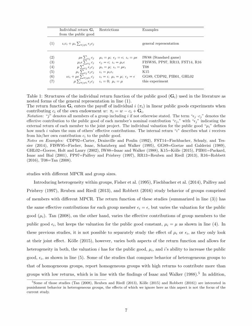
Table 1: Structures of the individual return function of the public good (Gi) used in the literature asnested forms of the general representation in line (1).The return function Gi enters the payoff of individual i (πi) in linear public goods experiments whencontributing ci of the own endowment w: πi = w − ci + Gi.Notation: “j” denotes all members of a group including i if not otherwise stated. The term “εj · cj” denotes theeffective contribution to the public good of each member’s nominal contribution “cj ,” with “εj” indicating theexternal return of each member to the joint project. The individual valuation for the public good “µi” defineshow much i values the sum of others’ effective contributions. The internal return “ι” describes what i receivesfrom his/her own contribution ci to the public good.Notes on Examples: CDP92=Carter, Drainville and Poulin (1992), FST14=Fischbacher, Schudy, and Tes-sier (2014), FISW95=Fischer, Isaac, Schatzberg and Walker (1995), GG89=Goetze and Galderisi (1989),GHL02=Goeree, Holt and Laury (2002), IW88=Isaac and Walker (1988), K15=Kolle (2015), PIB01=Packard,Isaac and Bial (2001), PP97=Palfrey and Prisbrey (1997), RR13=Reuben and Riedl (2013), R16=Robbett(2016), T08=Tan (2008).

studies with different MPCR and group sizes.

Introducing heterogeneity within groups, Fisher et al. (1995), Fischbacher et al. (2014), Palfrey and

Prisbrey (1997), Reuben and Riedl (2013), and Robbett (2016) study behavior of groups comprised

of members with different MPCR. The return function of these studies (summarized in line (3)) has

the same effective contributions for each group member εi = ε, but varies the valuation for the public

good (µi). Tan (2008), on the other hand, varies the effective contributions of group members to the

public good εi, but keeps the valuation for the public good constant, µi = µ as shown in line (4). In

these previous studies, it is not possible to separately study the effect of µi or εi, as they only look

at their joint effect. Kolle (2015), however, varies both aspects of the return function and allows for

heterogeneity in both, the valuation i has for the public good, µi, and i’s ability to increase the public

good, εi, as shown in line (5). Some of the studies that compare behavior of heterogeneous groups to

that of homogeneous groups, report homogeneous groups with high returns to contribute more than

groups with low returns, which is in line with the findings of Isaac and Walker (1988).5 In addition,

5Some of those studies (Tan (2008), Reuben and Riedl (2013), Kolle (2015) and Robbett (2016)) are interested inpunishment behavior in heterogeneous groups, the effects of which we ignore here as this aspect is not the focus of thecurrent study.

7

these studies observe that in heterogeneous groups, members with high ability contribute more than

those with low ability. Finally, Kolle (2015) observes that groups with heterogeneous abilities (εi)

contribute more on average than those with heterogeneous valuations (µi). These differences are driven

by low valuation types who reduce their contributions to less than half of the amount of high valuation

types. However, when members differ in their ability to contribute, low ability types contribute more

than double compared to low valuation types, but still slightly less than high ability types. Given this

empirical evidence, one might conclude that individuals react positively to an increase in the MPCR.

The drawback of these studies is that it is impossible to identify whether the motivation to increase

contributions originates from higher returns or from lower costs of contributing. This identification

problem arises because internal and external returns are perfectly correlated, i.e., a higher MPCR

(µiεi) directly implies lower marginal net costs of contributing (1-µiεi). In our experimental design,

we aim at solving this identification problem and investigate the effect of returns in heterogeneous

groups isolated from the costs of contribution. To achieve this goal, we build on the public goods

literature that varies independently the internal and external returns and is summarized in line (6) of

Table 1. Contrary to the literature presented so far, this stream of research makes a precise distinction

between the “internal return” and the “external return” from the public good. Yet, the existing studies

examine the separate effect of internal and external returns only in homogeneous groups, where all

members have the same internal and the same external return (ιi = ι; µi = µ; εi = ε).

Goetze and Galderisi (1989) and Carter et al. (1992) compare groups that have either low or high

internal and low or high external returns in a 2x2 between-subjects design. Both studies find larger

contributions when external returns are high, suggesting that subjects react positively to the return

of the public good even when it only benefits others. Carter et al. (1992) find this effect to be present

in the last 5 periods of the experiment at a significance level of 0.01 but to have disappeared in the

last period.6 Packard et al. (2001) partly replicate Carter et al. (1992) and report that even when

internal returns are zero, behavior follows the general qualitative pattern in standard public goods of

substantial contributions in the first rounds followed by a decay in later rounds. They also find that

initial contributions of groups whose members have zero internal and non-zero external returns are

the same as those of groups with the same (non-zero) internal and external returns. However, the

contributions decay faster and contribution levels in the final rounds are significantly lower for groups

with zero internal return.

These three experiments employed low and high returns of similar magnitude across experiments

6Conditional on external returns, contributions are higher when internal returns are higher, although only Carteret al. (1992) find this effect to be significant.

8

– around 0.3 and 0.8 (and 0 for the internal return in Packard et al. (2001)) in a between-subjects

design with groups comprising four members. Subjects interacted only once, either in a one-shot

experiment or with rematching groups every period in all experiments, with the exception of Packard

et al. (2001), where the group composition remained the same for 10 periods. Finally, Goeree et al.

(2002) study one-shot within-subjects designs with 12 treatments combining internal returns similar

to previous studies (either 0.4 and 0.8) but a wider range of external returns (0.4, 0.8, 1.2, and 2.4)

and groups with 2 and 4 members. They confirm earlier results that subjects react to an increase of

the external return by contributing more. To sum up, these four studies provide evidence that persons

in homogeneous groups react positively to external returns, even when internal returns are low – even

as low as zero.

The current article bridges the two branches of literature – (i) group heterogeneity in MPCR and

(ii) separating internal from external returns in homogeneous groups – by looking at heterogeneity in

external returns within groups. We keep the internal return constant for all group members and vary

only the external return that the contribution of a member generates for others, as shown in line (7)

of Table 1. Thus, different members in the same group vary in their external returns (εi 6= εj), but

have the same internal return (ιi = ι = 0). The important point of our design is that the internal

return is kept constant for all members which implies the same net costs of contributions. This design

allows us to isolate the effect of ability on contributions from that on own well-being in heterogeneous

groups. Importantly, it eliminates the confound of lower net costs for high ability types present in

previous studies and elucidates the driving force of contribution behavior in a heterogeneous public

goods environment.

Coming back to our orchestra example from the introduction, we can draw some links to our

design. If soloists and violinists participate in as many rehearsals and are paid the same for each

performance regardless of the time actually spent in rehearsals, their internal return of contributing

is the same as well as are their marginal net costs of rehearsal time. In reality, however, soloists did

not participate in as many rehearsal as violinists. They received the same pay for fewer hours of

rehearsing, compared to violinists. This relatively higher salary created tensions with the violinists,

even though management thought it to be justified because of the more effective contribution of the

soloists. The orchestra management argued that soloists are more vital for a performance. Actually,

whereas violinists took the point of equal net contribution costs as argument for demanding the same

pay per hour of rehearsal time, management questioned this assumption and brought into consideration

that net costs of soloists might be higher than that of violinists, due to, for example, higher stress and

thus needed compensation.

9

2.2 Information settings in public goods

External returns may affect contributions via the own preferences that arise solely as reaction to

changed incentives (e.g., efficiency concerns, altruism) or via more complex reflection taking own

and others’ incentives and contributions into account. As a consequence, information might very

likely affect the channel through which heterogeneity in external returns affects contribution behavior.

Therefore, in our study, we vary the information group members have about the return rates of others

to generate insight in contribution behavior in heterogeneous groups. Up to this point in time, little

is known about the effect that information has on contributions in public goods experiments. A few

studies exist that vary the aggregation level of the information that group members receive after each

round on others’ contributions (Sell and Wilson (1991), Croson and Marks (1998), Andreoni and Petrie

(2004)).7 Complementary, Marks and Croson (1999) look at the information about the distribution

of valuations for the public good in groups whose members vary in their valuations.

Sell and Wilson (1991) find that information on individual contributions of other group members

increases average contributions – compared to providing information on aggregate contributions, or

no information at all – and suggest that such behavior can partly be explained by the fact that trigger

strategies and positive reinforcement can be better applied when information on individual contribu-

tions is available. These strategies can only be applied when group members interact repeatedly, thus

with a partner matching protocol, where the same group members interact over several periods, but

not with stranger matching, where group composition changes after every period. Supporting evidence

for such behavior is reported in Cox and Stoddard (2015) who find more extreme behavior in a partner

matching compared to stranger matching when information on individual behavior is available instead

of aggregate contributions. Andreoni and Petrie (2004) and Croson and Marks (1998) find signifi-

cantly larger contributions when – in addition to providing information on individual contributions of

other group members – individual contributors can be identified, either by a digital photograph or by

subject ID numbers. Marks and Croson (1999) study threshold public goods games with three levels of

information that group members have about the valuations of others.8 Their results suggest that wit-

hout information on individual contributions of other group members, information on heterogeneous

valuations of the public good does not alter the aggregate level of contributions.

In contrast to this literature, we investigate the effect of various levels of information in a systematic

way. More precisely, we look at three conditions in which we vary the information group members have

7In the field, Ayres et al. (2012) look at the effect of information about energy usage of peers on energy consumption.They report high energy consumers to reduce their consumption after learning about others’ consumption.

8In all conditions, subjects only knew whether the sum of all contributions was above the threshold, in which casethe public good was provided. Otherwise, every contributor was reimbursed his or her contribution.

10

about the heterogeneity of the external returns in the group, but always provide information about

individual (nominal) contributions of others. In the baseline treatment, group members are informed

about their own internal and external return as well as individual nominal contributions of others in the

previous periods. In the other two treatments, participants are additionally informed about the internal

and external returns of other group members. Furthermore, only in the third treatment, participants

are informed about which type made a particular contribution. This design allows us to control the

level of information about heterogeneity in the external return and to systematically examine how the

structure of information affects voluntary contributions in a heterogeneous environment.

3 The experiment

The experiment was designed to uncover the effect of the external return on contributions to public

goods in heterogeneous groups. We exploit the variation in the information about the heterogeneity

that group members have to isolate the social norms applied in heterogeneous environments. We

explain the payoff function in more detail in section 3.1. Each group faces one of three information

conditions about the external returns in the group, which we present in section 3.2 below.

3.1 Payoff function

In the experiment, each of the n group members has to decide how to divide the personal endowment

w between a private account and a group account. Each unit that a member i allocates to the private

account generates a return of one, and each unit that i contributes to the public good ci generates an

internal return from the public good of ι for i. Thus, the net costs for i of contributing a unit to the

public good are 1− ι. But i’s contribution also generates an external return for other group members.

And vice versa, i benefits from the external returns generated by other group members’ contributions

to the public good. Thereby, we distinguish between the external return εj that indicates by how

much a unit contributed by member j increases the public good for others, and the external individual

return µεj , that refers to how much i (and others except j) benefit from another group member’s

contribution. There are two external return types with equal representation of each type in the group:

a low ability type (εL), hereafter referred to as L-types, and a high ability type (εH), hereafter referred

to as H -type. The payoff function of group member i can be summarized as follows:

πi = w − ci + ιci + µn∑

∀j 6=i,kεjcj

with ε ∈ {εH , εL}, H ∈ {1, . . . , n/2}, L ∈ {n/2 + 1, . . . , n}, εi 6= εk; i, k ∈ {1, . . . , n}

11

As pointed out in section 2.1, in standard public goods experiments, internal returns equal external

individual returns and are referred to as marginal per capita return (hereafter referred to as MPCR =

ιi = µ · εi). Heterogeneity in MPCR introduces also heterogeneity in the costs of contributing to the

public good. For example, one unit contributed by a person with a high MPCR increases the public

good more than a one unit contribution from a person with a low MPCR as MPCRH > MPCRL.

At the same time, the net costs of the same effective contribution to the public good is lower for a

person with a high MPCR compared to a person with a low MPCR (1−MPCRH < 1−MPCRL).

These two simultaneous effects of heterogeneity in MPCR make it difficult to identify whether persons

with high returns contribute more because they increase the public good more effectively or because

their costs are lower. The separation of MPCR in internal and external return enables us to introduce

variation in the ability to contribute to the public good via the external return while keeping the

internal return and thus the costs of contribution constant across types.9

It is important to notice, however, that keeping the internal returns constant across types, but

allowing each member to benefit from the contributions of all other group members would lead to an

asymmetric payoff structure, as each member always benefits from contributions of fewer members

of the own type, and more members of the other type.10 Kolle (2015) emphasizes the importance of

symmetry in the payoff function in public goods games when every member contributes the same net

amount of tokens, which would not be the case in our experiment when a member benefits from all

other members’ contributions. As we want contributions not to be influenced by an asymmetric payoff

function but solely by the change in the external return, we exclude the contributions of a person

with an opposite type such that every member benefits from the contributions of an equal number of

both types. Thus, we assure a symmetric payoff structure in our experiment. In addition, we set the

internal return to zero ι = 0 for all members in all groups.11

9In fact, Carter et al. (1992) and Goeree et al. (2002) have shown in the case of homogeneous groups that contribu-tions are sensitive to both, external and internal returns. We concentrate solely on the effect of external returns, i.e.,contributions benefiting only others, and vary those marginal benefits within groups while we keep private costs via theprivate benefits of contributing constant across individuals.

10If all members contributed the same nominal amount in our experiment, then H-types would have lower payoffs, asthey benefit from contributions by less H-types, whereas L-types would receive a larger return from the public good, asthey benefit from the external return of one more H-type’s contribution. Consider a group composed of six members;three L-types and three H -types. While all would benefit the same from their own contribution when the internal returnis the same across types, in addition, H-types would benefit from contributions of three L-types and only two H-types, incontrast to L-types who would benefit from contributions of two L-types and three H-types. As the marginal contributionof H-type members increases the public good by more than that of L-types, L-types receive a larger return from thepublic good.

11Surely, this feature creates a discrepancy between our design and the orchestra example. As explained before, wemake this design choice purely in order to isolate the effect of ability on increasing the public good from the net costsof contributing. Packard et al. (2001) also studied such boundary case with ι = 0 in homogeneous groups. As internalreturns were zero, they interpreted contributions as purely altruistic and reciprocal because they exclusively benefitothers. Packard et al. (2001) emphasize the importance of such boundary designs, which are not necessarily meant

12

These considerations explain the particularity of how we set up the payoff function and calculated

external returns. The sum of the effective contributions to the public good from other group members,∑∀j 6=i,k εjcj , restricts i to benefit from contributions of n−2 members. The two members from whose

contribution i is excluded are, first, the member i itself, because of an internal return of zero and,

second, another member k with a type opposite to that of i (εi 6= εk), because of the symmetry of the

payoff function. Restricting the benefits to contributions from fewer members but the same number

of L-types and H-types ensures symmetry of the payoff structure for the returns from the public good

across members.

In the experiment, there are n = 6 group members, three members per type. The external returns

are εL = 1.33 for L-types and εH = 3.99 for H-types. All members have the same valuation and benefit

from effective contributions of four other group members (µ = 1/4) (excluding themselves and another

randomly selected group member with an opposite type). Therefore, external individual returns for a

nominal contribution of L-types and H-types are µεL = 0.3325 and µεH = 0.9975, respectively. These

external individual returns are comparable to those employed by the other experiments reviewed in

section 2.1, which lay in the range between 0.3 and 2.4.

3.2 Information treatments

A group member stays the same type and interacts in the same group repeatedly over 15 periods.

After each period, all group members’ individual nominal contributions to the project are revealed

anonymously to the whole group. Our treatment variable, the level of information, varies in two ways:

first, subjects either do or do not receive information on the distribution of types within the group,

and second, the feedback information about the nominal contributions of all group members does or

does not identify contributors by their type. We study the following information scenarios that are

summarized in the top part of Table 2.

In the No-info treatment, subjects know their own type, i.e., they are informed about their own

external return, but not the distribution of external return types within their group.12 In the Part-info

and Full-info treatments, the distribution of types is explicitly stated in the instructions. Additionally,

to replicate 100% of a real world situation, rather to isolate and focus on particular factors of interest. Nevertheless,Packard et al. (2001) provide a real world example with zero internal returns of public good contributions: They figurea homeowner who cleans up parts of her garden that is in sight of her neighbors, but not in her own, implying internalreturns of zero for cleaning up this part of her garden. However, if everybody cleans also these spots of the garden thatare not visible to the owner but to their neighbors, everybody in the neighborhood will be better off.

12The instructions never used the word “ability” or “external return” and left open the possibility that differences inthe external return between group members may exist. While this approach implies loosing some control over groupmembers’ beliefs concerning other members’ types, it implements the No-info treatment, our benchmark treatment, ina way that is as close as possible to the other two treatments.

13

Informationabout ...

Treatments (between-subjects design)

No-Info Part-Info Full-Info

... externalreturns

Own type Own type and distribution ofexternal returns in group

... type ofcontributors

without identification ofcontributor’s type

with identification ofcontributor’s type

Descriptive Statistics: contributions

Mean 0.42 0.54 0.56(0.25) (0.28) (0.29)

Mean L-type 0.42 0.59 0.50(0.22) (0.28) (0.28)

Mean H-type 0.43 0.50 0.62(0.28) (0.27) (0.28)

Periods 15 15 15N subjects 54 54 54Total Nobs 810 810 810

Table 2: Summary of experimental design and descriptive statistics (mean contributions of both typesand by type - all as proportion of endowment, standard deviations in parenthesis, number of periods,number of subjects, and total number of observations.)

the feedback information in the Full-info treatment allows subjects to link an individual nominal

contribution to the contributor’s type. In sum, the three treatments gradually change the level of

information about the heterogeneity in the external return within the group and whether the type of

an individual contributor is known or not.

3.3 Experimental procedure

The computerized experiment (zTree, Fischbacher, 2007) took place at the laboratory of the Max

Planck Institute of Economics in Jena, Germany. A total of 162 undergraduate students (54 per infor-

mation treatment) from Jena University were recruited using an online recrutement system (ORSEE,

Greiner, 2004). Participants were on average 24 years old and 43% of them were men. In order to

capture some of the individual heterogeneity amongst participants that might influence the behavior

in the experiment, participants completed a standard personality questionnaire after the experiment,

resulting in a personality index for each participant.13 The personality index of our participants ranges

13We administered the revised version of the Sixteen Personality Factor Questionnaire (Cattell et al., 1993) in its officialGerman version by Schneewind and Graf (1998). In particular, our personality index is derived from the individual scorein the global personality scale that captures conscientiousness or self-control. This personality index reflects several

14

from one to nine with a mean value of 4.35.

Upon arrival and random seating in the lab, subjects received written instructions.14 Once all

subjects had finished studying the instructions, they answered some control questions to check their

understanding of the interaction in the experiment. After the questions had been correctly answered

by everyone, the experiment started. All group members decided about their contribution to the public

good, after which the computer calculated individual payoffs and informed group members about their

payoffs. Additionally, a history table was displayed containing the list of nominal contributions by

each group member in all previous periods. The order of individual contributions in the history table

was randomized so that contributions could not be attributed to a specific group member.15 In the

Full-info treatment, the history table also displayed the type of each contributor.

At the end of a session, subjects received their payoff from the experiment and a show-up fee of

2.5 Euros in cash. Experimental earnings were counted in points and exchanged for Euros, with 80

points corresponding to 1 Euro. Subjects earned on average 5.7 Euros for the 15 rounds, which lasted

on average 30 minutes.16

3.4 Descriptive Statistics

In total, we observe 2,430 contribution decisions for the whole experiment, breaking down into 3 tre-

atments with 9 groups per treatment, each with 6 members who decide in every of the 15 periods how

much to contribute to the joint project. The bottom part of Table 2 reports the mean of the average

individual contributions over 15 periods as a proportion of the endowment. Across the treatments,

participants contribute about 50 percent of their endowment. The average contributions in the tre-

atments Part-info and Full-info appear to be slightly higher than that in the No-info treatment.17

Mean contributions by type appear to be similar for both types in the No-info treatment (L-type: 0.42,

H-type: 0.43, Signed ranks test: p-value = 0.51), but appear to differ for the other two treatments.

traits that are associated with the tendency to rely on rules and socially accepted behavior (Conn and Rieke, 1994). Theindex is expressed in sten-scores that can range from one to ten. Sten values are derived from comparing test scores tothe results of a norm population. The average (expected) sten-value in the German population is 5.5 with a standarddeviation of 2, whereby higher sten-values indicate higher awareness and personal reliance on societal norms and rules.

14A presents a translation of the original German instructions.15Participants were informed that they benefit from contributions of “four other group members” (No-info treatment)

and “two of each type” (Part-info and Full-info treatment), but they were not informed about which of the displayednominal contributions they benefited from. Therefore, in the Part-info treatment, it was hardly possible to infer thetype of the contributor from displayed nominal contributions, or, similarly, to deduce in the No-info treatment that therewere different types.

16Each session consisted of two phases each lasting 15 periods. In the second phase, groups were confronted with oneof the two other treatments in order to study path dependency of contribution behavior. In this article, we consider onlythe first phase. Average earnings for the whole experiment (including both phases) were about 11 Euros.

17Ranksum tests comparing contributions of Part-info and No-info, and those in Full-info and No-info result in p-valuesof 0.23 and 0.20, respectively.

15

Aggregated average contributions of L-types are higher in the Part-info treatment and lower in the

Full-info treatment compared to those of H -types.18

The dynamics in the experiment are shown in Figure 1. The upper panel plots the average con-

tribution as a share of the endowment by treatment across the 15 periods. In all three treatments,

the average contribution generally decreases over the course of the experiment, with a stronger decay

towards the end. There are noticeable differences across the treatments in how contribution behavior

evolves over time. In the No-info treatment, the general trend of contributions is downward sloping,

a behavior that is in line with observations in other public goods experiments. In contrast, in the

other two treatments with information about heterogeneity, average contributions seem to increase

initially before following the general trend of decay. The lower panel of Figure 1 shows the average

contribution as a share of the endowment by types across the 15 periods, separately for each treatment.

Again, contributions of the two types appear to be similar in the No-info treatment. In Part-Info,

L-types contribute slightly more than H-types in nearly every round, while in Full-info the pattern is

reversed.19 In the following, we estimate an empirical model of contribution behavior that allows us

to exploit the information at the individual level.

4 Empirical model of contribution behavior

In this section, we present a random effects Tobit model in order to quantify the effect of information

and external return on contribution behavior over time while controlling for individual heterogeneity.

The choice of the empirical model is guided by the dynamic nature of the data and the fact that

contributions are bounded below and on top. Our model allows individual contributions to depend

not only on the treatment variables, but also on observable and unobservable personal characteristics

as well as time. This way, we are able to provide statistical evidence of how information about

heterogeneity affects behavior and to gain more insight on how individual contributions evolve over

time.

In our model, we describe the share that individual i contributes from his or her own endowment

18Aggregation of contributions per group leaves us with 9 observations per treatment and allows us to perform standardnon-parametric tests. Wilcoxon signed ranks tests that account for the dependencies of types within groups, however,cannot reject the null hypothesis that types make the same contributions at conventional levels of significance ( p = 0.11 inPart-info treatment and p = 0.26 in Full-info treatment). The lack of significant variation in the analysis of aggregateddata is not surprising. Though necessary for appropriate non-parametric testing, aggregation neglects informationcontained in individual data. It is very likely that information exerts its effect through dynamic interaction over time.

19B includes supplementary analyses of the group average contributions of the three treatments for each period (Table4) and of the group average contributions by type for each period in each treatment (Table 5).

16

No-info Part-info, Full-info,

0 5 10 15

0.25

0.50

0.75

1.00No-info Part-info, Full-info,

No-info, High No-info, Low

0 5 10 15

0.25

0.50

0.75

1.00No-info, High No-info, Low Part-info, High Part-info, Low

0 5 10 15

0.25

0.50

0.75

1.00Part-info, High Part-info, Low Full-info, High Full-info, Low

0 5 10 15

0.25

0.50

0.75

1.00Full-info, High Full-info, Low

Figure 1: Upper panel: Average nominal contributions as share of the endowment for the threetreatments (No-info, Part-info and Full-info) Lower panels: Average nominal contributions as shareof the endowment for the external return types (High- and Low -types)

in period t, y?it, as a function:

y?it = γ0 + γ1Part-infoi + γ2Full-infoi + hiω + f(t) + xiβ + uit (3)

where γ0 indicates the basic contribution level. We capture the influence of different levels of informa-

tion about heterogeneity in the external return by treatment dummies, with the No-info treatment as

a baseline. Parameter γ1 measures the influence of information about heterogeneity and γ2 measures

the effect when external return can be additionally linked to specific contributions. Part-infoi (Full-

infoi) are dummy variables indicating the treatment in which i participated. The vector h contains a

dummy variable for the type (Highi = 1 if i is a H -type and zero otherwise) and interaction terms of

the type with the treatments. The parameter vector ω measures the effect of types across treatments.

We control for time trends by including f(t), a function of time. The vector xi represents individual

observable characteristics (age, gender, personality index). Their influence on contributions is captu-

red by the parameter vector β. Idiosyncratic errors, uit, are assumed to be independent of type and

17

other individual characteristics in xi.

Given the design of the experiment, individual contributions to the joint project are doubly censo-

red, first at the lowest contribution level of 0 units and second at the highest contribution level of 17

units, the endowment in each period.20 As we define our variable of interest, the contribution to the

public good as a share of the endowment, censoring is between 0 and 1. We therefore use a standard

regression doubly censored Tobit model to estimate the relation for the latent proportions y?it that a

group member i contributed (ci/w) described in model (3) with

yit

= 0 if y?it ≤ 0,

= y?it if 0 < y?it < 1,

= 1 if y?it ≥ 1.

(4)

We estimate four specifications of the model in equation (3).21 The first specification includes only

treatment dummies for the different information conditions. The second looks only at the two types.

The last two specifications control for both treatments, types, and their interaction. All specifications

include the same set of background characteristics. The first three specifications model the time

trend non-parametrically by including dummy variables for each period (f(t) = δt1t with 1t being an

indicator function for period t, for t > 1 and f(1) = 0). We find an inverse-U relation between time

and the contributions to the joint project. Therefore, in the last specification, we model the time

trend as a quadratic polynomial that includes interaction effects with types and the three information

conditions:22

f(t) = τ10 · t+ τ20 · t2 + Interaction(t,Highi,Part-infoi,Full-infoi). (5)

Parameterizing the time as quadratic polynomial allows us to account for both linear and non-linear

effects of time as well as to include interactions with the different information conditions while mini-

mizing the loss of degrees of freedom.

20In fact, 23% and 21% of all contribution decisions are at the upper and lower limits, respectively.21We thank Charles Bellemare for providing his tobit model OX code.22The detailed time function is given by:

f(t) = τ10 · t+ τ11 · t · Part-infoi + τ12 · t · Full-infoi+ τ13 · t ·Highi + τ14 · t ·Highi · Part-infoi + τ15 · t ·Highi · Full-infoi+ τ20 · t2 + τ21 · t2 · Part-infoi + τ22 · t2 · Full-infoi+ τ23 · t2 ·Highi + τ24 · t2 ·Highi · Part-infoi + τ25 · t2 ·Highi · Full-infoi

18

5 Results

In this section, we present the estimation results of the four specifications introduced above. Specifica-

tion (1) estimates the effect of the information conditions on contributions without controlling for the

type. Specification (2) complements these results and estimates only the effect of types. Specification

(3) controls for both, information conditions and types as well as their interaction. Specification (4)

models the time trend as a quadratic polynomial, instead of using time dummies as did the Specifi-

cations (1) to (3), and adds interaction effects with the treatment variables and time. Furthermore,

we present in this section the marginal effects of type and information on contributions. We also

investigate whether and how types react differently to the distinct levels of information.

5.1 Parameter estimates

Parameter estimates of the main variables are presented in Table 3 and parameter estimates for the

time trend of Specifications (1) to (3) in Table 6 in C. Specification (1) indicates that contributions are

significantly smaller in the No-info treatment than in the other two treatments. However, there seems

to be no difference in contributions between the two treatments with more information. Specification

(2) singles out the effect of the external return on contributions, which is positive. However, even

though the effect is significantly different from zero, it is rather small.

The estimated parameters of Specification (3) indicate that information about heterogeneity has

a significantly positive impact on contributions (γ1, γ2 > 0).23 Whereas the general propensity to

contribute with little information (γ0) and the increase to contribute with partial information (γ1)

remain almost of the same magnitude as in Specification (1), the increase of nominal contributions in

the Full-info treatment is now only half of the increase in the Part-info treatment. Controlling for

information reveals that the positive effect of external returns on contributions comes exclusively from

the Full-info treatment environment.

The three specifications control for background characteristics and for the time trend with period

dummies. We find that women tend to make significantly lower contributions (β2 < 0) and that age

and the personality index have significant but relatively small negative effects on contributions. All

effects are significant at p = 2.5% or less. The influence of background characteristics on contributions

is robust across specifications. The period dummy coefficients reveal an inverse U-shaped time trend,

23In the Full-info treatment, this increase is almost exclusively driven by the H -type (γ2 < ω2). In the No-infotreatment, H -types contribute significantly less than their L-type peers (ω0 < 0), but the size of the effect is relativelysmall and there is practically no difference in this respect when looking at the Part-info treatment (ω1 not significantlydifferent from zero).

19

indicating an increase in contribution levels until period three and a strong decrease over the last three

periods of the experiment. Specifications (1) and (2) are nested in Specification (3). The loglikelihood

values of the three models indicate that the model of Specification (3) fits much better our experimental

observations.24

Specification (4) models the time trend as a quadratic polynomial, as in equation (5), allowing us

to control for more interaction effects while minimizing the loss in degrees of freedom. The unobserved

heterogeneity in Specifications (1) and (2) is about twice the size of the one in the other two Specifica-

tions (3) and (4), where we control separately for the influence of information and external return as

well as their interaction and time effects. However, Specification (4) still seems to fit better our expe-

rimental observations than Specification (3). The Akaike Information Criterion (AIC) (Akaike (1974))

allows us to compare the goodness-of-fit between the two specifications: the AIC of Specification (3)

is 66391.4 and the AIC of Specification (4) is 66353.4. Thus, the relative likelihood of Specification

(3) is very low compared to Specification (4).25,26 We continue to work with the latter.

Specification (4) has the advantage of controlling for the interaction of the time trend and the

information conditions. The results reveal that the effect of information materializes largely through

dynamic interactions over time and that this effect varies by type. More precisely, information about

heterogeneity has a non-linear effect on individual contributions of both types. Instead of the standard

monotonic decay, contributions increase before they diminish (τ11, τ12 > 0 and τ21, τ22 < 0). Moreover,

additional information counterbalances the declining trend for contributions of H -types (τ24, τ25 > 0).

These parameter estimates are not individually significant. In order to test whether their joint effect

is significant and to assess the global picture of these individual interactions, we compute expected

contributions and calculate marginal effects using our estimated parameters.

5.2 Marginal effects on contributions

In this section, we present the marginal effects estimations based on the parameter estimates from

Specification (4). The details of how we computed the marginal effects are presented in D.

24Loglikelihood ratio tests: Specification (1) vs (3): p = 0.00, Specification (2) vs (3): p = 0.00.25The relative likelihood of Specification (3) is exp((66353.4 − 66391.4)/2) = 0.00056 · 10−5.26In section 5.2, we present our marginal effects analysis of Specification (4). Additionally, we present the marginal

effects based on Specification (3) in E. A comparison of the marginal effects predictions of both specifications with theempirical observations confirms also visually a better fit of Specification (4) with the data.

20

Sp

ecifi

cati

on1

Sp

ecifi

cati

on2

Sp

ecifi

cati

on3

Sp

ecifi

cati

on4

Var

iab

leP

ara

met

erC

oeffi

cien

tT

-val

ue

Coeffi

cien

tT

-val

ue

Coeffi

cien

tT

-val

ue

Coeffi

cien

tT

-val

ue

Con

stant

γ0

0.86

9.69

1.02

10.7

70.

848.

950.

935.

93P

art

-in

foγ1

0.20

16.8

90.

2112

.30

0.09

0.43

Fu

ll-i

nfo

γ2

0.24

21.7

20.

105.

960.

020.

12H

-typ

eω0

0.05

4.33

-0.0

4-2

.42

-0.0

3-0

.12

H-t

yp

eP

art

-in

foω1

-0.0

1-0

.50

0.04

0.12

H-t

yp

eF

ull

-in

foω2

0.29

12.8

00.

331.

20li

nea

rte

rmof

the

Tim

etr

end

τ 10

0.01

0.28

Part

-in

foτ 1

10.

061.

02F

ull

-in

foτ 1

20.

050.

89H

-typ

eτ 1

30.

010.

14H

-typ

eP

art

-in

foτ 1

4-0

.07

-0.7

6H

-typ

eF

ull

-in

foτ 1

5-0

.03

-0.3

9qu

adra

tic

term

ofth

eT

ime

tren

dτ 2

0-0

.00

-0.8

6P

art

-in

foτ 2

1-0

.00

-1.2

5F

ull

-in

foτ 2

2-0

.00

-1.1

7H

-typ

eτ 2

3-0

.00

-0.2

9H

-typ

eP

art

-in

foτ 2

40.

001.

11H

-typ

eF

ull

-in

foτ 2

50.

000.

55A

geβ1

-0.0

1-5

.35

-0.0

1-6

.64

-0.0

1-4

.85

-0.0

1-4

.84

Gen

der

β2

-0.2

5-2

2.83

-0.2

4-2

1.01

-0.2

4-1

9.91

-0.2

4-1

9.84

Per

son

alit

yin

dex

β3

-0.0

3-1

0.56

-0.0

3-1

0.29

-0.0

3-9

.24

-0.0

3-9

.28

Tim

ed

um

mie

sY

esY

esY

esN

oN

um

ber

ofO

bse

rvati

on

s24

3024

3024

3024

30N

um

ber

ofP

aram

eter

s21

1923

21

σε

-1.0

7-6

3.5

-1.0

3-6

1.38

0.58

62.5

40.

5864

.14

Log

-Lik

elih

ood

valu

e-3

3431

-339

31-3

3173

-331

56

Tab

le3:

Est

imati

on

resu

lts

for

nom

inal

contr

ibu

tion

beh

avio

r(d

epen

den

tva

riab

le:

nom

inal

contr

ibu

tion

asa

shar

eof

the

end

owm

ent)

.

21

External return

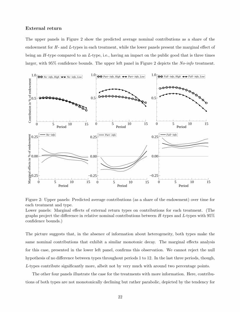
The upper panels in Figure 2 show the predicted average nominal contributions as a share of the

endowment for H - and L-types in each treatment, while the lower panels present the marginal effect of

being an H-type compared to an L-type, i.e., having an impact on the public good that is three times

larger, with 95% confidence bounds. The upper left panel in Figure 2 depicts the No-info treatment.

0 5 10 15

0.5

1.0

Period

Full−info, High Full−info, Low

0 5 10 15

0.5

1.0

Period

Part−info, High Part−info, Low

0 5 10 15

0.5

1.0

Period

Con

trib

utio

n in

% o

f en

dow

men

t No−info, High No−info, Low

0 5 10 15

−0.25

0.00

0.25

Period

Mar

gina

l eff

ects

in %

of

endo

wm

ent No−info

0 5 10 15

−0.25

0.00

0.25

Period

Part−info

0 5 10 15

−0.25

0.00

0.25

Period

Full−info

Figure 2: Upper panels: Predicted average contributions (as a share of the endowment) over time foreach treatment and type.Lower panels: Marginal effects of external return types on contributions for each treatment. (Thegraphs project the difference in relative nominal contributions between H -types and L-types with 95%confidence bounds.)

The picture suggests that, in the absence of information about heterogeneity, both types make the

same nominal contributions that exhibit a similar monotonic decay. The marginal effects analysis

for this case, presented in the lower left panel, confirms this observation. We cannot reject the null

hypothesis of no difference between types throughout periods 1 to 12. In the last three periods, though,

L-types contribute significantly more, albeit not by very much with around two percentage points.

The other four panels illustrate the case for the treatments with more information. Here, contribu-

tions of both types are not monotonically declining but rather parabolic, depicted by the tendency for

22

average contributions to increase initially before following the standard pattern of decay. Moreover,

from the lower middle and lower right panels, we learn that contribution behavior differs significantly

between types and also between the Part-info and the Full-info treatments.

The upper and lower middle panels illustrate behavior in the Part-info treatment. There, the

predicted average contribution of L-types is higher than that of H -types by about 5% to 10% of the

endowment. The difference in contribution behavior between H - and L-types is reversed in the Full-info

treatment, which is illustrated in the upper and lower right panels of Figure 2. When contributions can

be linked to the type of the contributor, H -types give significantly more than L-types. The difference

amounts to around 15% of the endowment and remains constant over time as contributions of both

types follow the same time trend.

Information by type

Providing information about heterogeneity obviously affects contribution behavior of types in different

ways. To test the significance of information on contributions separately for both types, we compute

marginal effects presented in Figure 3, for H -types in the upper panels and for L-types in the lower

panels.

The upper left panel shows that H -types contribute more in the second half of the experiment

when they have information about the heterogeneity than in case they do not have this information.

When all group members can additionally link contributions to types as shown in the upper right

panel, H -types contribute between 10 and 20 percent more of their endowment. However, this effect is

decreasing over time, and in the last two periods, contributions no longer differ significantly. Finally,

the upper middle panel indicates that H -types’ contributions are around 20 percent higher when they

have information about heterogeneity and contributions can be linked to types than in case where

they have no information. This effect is relatively stable over time.

We find very different marginal effects for L-types, shown in the lower panels of Figure 3. The lower

left and middle panels indicate that information on heterogeneity generally increases the contributions

of L-types. The effect is about two times stronger when only information about heterogeneity (lower

left panel) is available than in the situation where contributions can be linked to the type (lower middle

panel). The difference between both effects is significant and visualized in the lower right panel that

depicts the difference between the two treatments with partial and full information.

Finally, we repeated the marginal effects analysis using parameter estimates from Specification

(3). We present these two figures, Figures 4 and 5, in E together with a third set of figures, Figures 6

23

0 5 10 15

−0.25

0.00

0.25M

argi

nal e

ffec

ts in

% o

f en

dow

men

t

Period

High: Part vs. No−info

0 5 10 15

−0.25

0.00

0.25

Period

High: Full vs. No−info

0 5 10 15

−0.25

0.00

0.25

Period

High: Full vs. Part−info

0 5 10 15

−0.25

0.00

0.25

Period

Mar

gina

l eff

ects

in %

of

endo

wm

ent Low: Part vs. No−info

0 5 10 15

−0.25

0.00

0.25

Period

Low: Full vs. No−info

0 5 10 15

−0.25

0.00

0.25

Period

Low: Full vs. Part−info

Figure 3: Marginal effects of information on contributions separately for H -types and L-types. (Thegraphs project the difference in relative nominal contributions between two information scenarios with95% confidence bounds.)

and 7, in F presenting the same differences based on average data. A comparison of these three sets

of figures demonstrates that Specification (4) captures the dynamic evolution of contributions over

time much better than Specification (3). These comparisons confirm our choice of Specification (4)

as the main model for our analysis and underline the importance of the interaction of time with the

treatment variable and the type.

6 Summary of the results and discussion

In this section, we summarize our three main results and discuss them in more detail in light of the

existing literature. Our first finding is that (1) heterogeneity in the ability to provide the public good

does not affect nominal contributions when no information on heterogeneity is provided. Second, we

observe that (2) nominal contributions increase with ability when members are aware of the heteroge-

neity and contributions can be linked to the ability type. Yet, we find, third, (3) nominal contributions

to be inversely related to ability, when group members are only aware of the heterogeneity but cannot

24

link contributions to the type.

Our first result in connection with our second indicates that contributions vary by type and in-

formation scenario, a finding which expands our knowledge about the effects of return rates in hete-

rogeneous groups in the literature. This literature presumed so far that members of heterogeneous

groups react solely to their own marginal per capita return. Such evidence is provided by individual

decision experiments on altruism (Andreoni and Miller (2002), Karlan and List (2007)) and public

goods experiments with different marginal per capita return between homogeneous groups and within

heterogeneous groups (see Section 2.1). These papers demonstrate that individuals react to changes in

the efficiency of their contributions. Their findings are qualitatively in line with ours when members

have information on the heterogeneity in the group and the contributor’s type, which in fact are the

information conditions used in the literature. However, if solely altruism or warm glow are driving

the behavior in public goods experiments, group members should react exclusively to their external

return, i.e., by how much their contributions benefit others, independent of their knowledge about the

environment. We find, however, that H-types contribute more in the most transparent information

condition. Thus, information about the heterogeneity in the external return is important and drives

behavior in such environments. Furthermore, social norms in connection with efficiency concerns are at

play rather than altruism alone when members with high external returns make larger contributions.

The findings in this paper are – to the best of our knowledge – the first evidence that group

members react to the external returns their peers have and not only to the external returns of their own

contributions. In a way, our results push the concept of conditional cooperation (Fischbacher et al.

(2003)) a bit further, suggesting that persons have multiple dimensions of conditional cooperation.

They not only condition on others’ nominal contributions, but also on other factors, in our case

ability, in other words, how efficiently contributions affect the joint project. The findings suggest

that peer pressure exists on the most able types, when sufficient information is available. This result

enhances our understanding of behavior in groups whose members vary in their ability to contribute

to a joint project and finds no equivalent in the existing public goods literature.

Our second result states that the positive effect of external returns in heterogeneous groups is

grounded in sufficient information on the environment. This result corroborates and extends findings

of a strand of the existing public goods literature that is concerned about the effect of returns on

contributions. This literature looks exclusively at environments in which group members have full

information on contributions and return rates of other members (see section 2.1). One main result

of this literature constitutes that individuals react to external and internal returns. Some researchers

vary the marginal per capita return for individuals in a group, i.e., internal and external return are

25

the same for an individual but vary between members of a group. Others vary internal and external

returns separately and study their variation in homogeneous groups. Our experiment combines both

approaches in that we allow internal and external returns to be distinct for individual members of

heterogeneous groups. Thereby, we avoid the confounding effect of diverging net contribution costs

among heterogeneous group members, which the hitherto literature has neglected. From our second

result we can add to the literature the insight that the existing finding of a positive relation between

external returns and contributions is in part due to the full information structure employed in these

experiments. We can add further that the established finding on the effects of heterogeneous marginal

per capita returns is robust to the cost of contribution.

Our third result, probably the most surprising one, indicates that only an environment with rather

detailed information induces efficient contributions. Thus, the finding in the previous literature that

high ability types contribute more than low types does not always hold and even reverses when less

information is provided, i.e., when members are informed about the heterogeneity in the group, but

it is not possible to link individual contributions to the ability type. In this case, low ability types

contribute significantly more than high types. This evidence, together with the observation that

H-types contribute more when information on the contributor’s type is available than when it is

not, seems to accord with the “poisoning-of-the-well” effect introduced by Fisher et al. (1995).This

effect refers to lower contributions of types with high marginal per capita return in heterogeneous

groups compared to their contributions in homogeneous groups.27 Under our different information

scenarios, we find that partial information about heterogeneity results in the “poisoning-of-the-well”

effect, whereas it is ceased under full information. Hence, we replicate what Fisher et al. (1995) call

a “curious phenomenon” that the “poisoning-of-the-well” effect disappeared when the experimenters

emphasized more strongly the heterogeneity in the groups to their participants, highlighting themselves

the importance of information (p.265, footnote 11). Despite this anecdotal evidence, our study is to

the best of our knowledge the first systematic investigation with heterogeneous groups under different

information scenarios, hence, the first to report such reversion in contribution patterns by different

types of external returns.

In a nutshell, we find an effect of external returns on contributions to joint projects in heterogene-

ous groups when group members have full information about each other. There is strong evidence in

27In Fisher et al. (1995) “the well” are types with a high rate of marginal per capita return, i.e., those with highinternal and high external rates of return. They are “well” or “better off” than others as they benefit from their owncontribution via the high internal rate of return and have, hence, lower relative costs to contribute compared to lowtypes. The “well” characterizes less precisely high types in our experiment, who have higher external returns but zerointernal returns, hence they are “only” more “able” to increase the public good for others, but cannot benefit from theirown contribution.

26

laboratory experiments and field studies that information about others affects contribution to public

goods (see section 2.2). In observing homogeneous groups, Andreoni and Petrie (2004) find an increase

in contributions when individual contributions can be identified. They suggest that individuals com-

pare their own contributions to some standard that can be established when contributions of others

are known. As information is likely to foster social comparisons and to clarify a standard, it is not

surprising that individuals react to available information. Such a standard may represent a social

norm, but which norm is established in groups with heterogeneous agents is an empirical question, to

which our paper provides some evidence.

Our results complement those of Andreoni and Petrie (2004) by adding the aspect of heteroge-

neity. We find that in heterogeneous groups types react differently to changes in the information

about heterogeneity and to changes in the information about the type of the contributor. From the

literature on fairness and justice norms one can derive different contribution norms for heterogeneous

environments, based either on efficiency or equity (Konow (2003)). By revealing the type-identity of

contributors, type specific standards or norms can arise more easily, which gives an idea – at least

empirically – of what norm is in place in groups with members who differ in their abilities. Given our

results, it seems that the standard emerging in our setting is that of efficient contributions, with high

ability types making higher nominal, hence, effective contributions. Our experimental results suggest

that efficiency motives emerge with sufficient information and social exposure: when identification of

ability is linked to individual contributions, high ability types contribute more compared to a situation

when group members are not informed about the heterogeneous abilities in the group.

7 Conclusion

This study explores the relationship between external returns, or the ‘ability to increase the value of a

joint project for others,’ and the level of available information on the return type of all group members

in the context of public goods production by groups whose members vary in their external return. Our

results not only extend the literature but shed new light on the existing results. We conjecture from

our findings that efficient contributions by high ability group members represent a social norm rather

than a reaction to increased incentives to contribute. Thus, efficient contributions are more likely in

environments with social approval or social pressure, for example when the identity of the contributor

is revealed. Whether efficiency is the most desirable norm from the point of view of a policy maker or

group members themselves is another important question left for future research.

We conclude by noting that the level of information about heterogeneity is crucial to understand

27

how heterogeneity in groups affects the provision of public goods. We consider our findings important

when deciding on the information to be transmitted in teams, for example about the (nominal) per-

formance of individual team members, or when evaluating different disclosure practices of fund raising

agencies.

References

Akaike, H.: 1974, A new look at the statistical model identification, IEEE Transactions on AutomaticControl 19, 716–723.

Andreoni, J.: 1988, Privately provided public goods in a large economy: The limits of altruism, Journalof Public Economics 35, 57–73.

Andreoni, J.: 1990, Impure altruism and donations to public goods: A theory of warm-glow giving,Economic Journal 100, 464–477.

Andreoni, J. and Miller, J.: 2002, Giving according to garp: An experimental test of the consistencyof preferences for altruism, Econometrica 70(2), 737–753.

Andreoni, J. and Petrie, R.: 2004, Public goods experiments without confidentiality: A glimpse intofund-raising, Journal of Public Economics 88, 1605–1623.

Ayres, I., Raseman, S. and Shih, A.: 2012, Evidence from two large field experiments that peercomparison feedback can reduce residential energy usage, The Journal of Law, Economics, andOrganisation. 29(5), 992–1022.URL: http://jleo.oxfordjournals.org/content/early/2012/08/18/jleo.ews020.full.pdf+html

Bellemare, C., Kroger, S. and van Soest, A.: 2008, Measuring inequality aversion in a heterogeneouspopulation using experimental decisions and subjective probabilities, Econometrica 76, 815–839.

Camerer, C. F.: 2003, Behavioral game theory, Princeton University Press, New Jersey.

Cappelen, A. W., Hole, A. D., Sørensen, E. Ø. and Tungodden, B.: 2007, The pluralism of fairnessideals: An experimental approach, American Economic Review 97(3), 818–827.

Carter, J. R., Drainville, B. J. and Poulin, R. P.: 1992, A test for rational altruism in a public-goodsexperiment, Working Paper Collage of the Holy Cross, Worcester, Massachusetts 01610, retrived inApril 2013 at: http://www.dklevine.com/archive/1a test f.pdf .

Cattell, R. B., Cattell, A. K. and Cattell, H. E. P.: 1993, 16 Personality Factors, Fifth Edition,Institute for Personality and Ability Testing, Champaign, Illinois.

Conn, S. R. and Rieke, M. L.: 1994, The 16PF Fifth Edition Technical Manual, Institute for Personalityand Ability Testing, Inc., Illinois.

Cox, C. A. and Stoddard, B.: 2015, Framing and feedback in social dilemmas with partners andstrangers, Games 6, 394–412.

Croson, R. T. A. and Marks, M. B.: 1998, Identifiability of individual contributions in a thresholdpublic goods experiment, Journal of Mathematical Psychology 42, 167–190.

28

Engelmann, D. and Strobel, M.: 2004, Inequality aversion, efficiency, and maximin preferences insimple distribution experiments, The American Economic Review 94(4), 857–869.

Fischbacher, U.: 2007, z-Tree: Zurich toolbox for readymade economic experiments, ExperimentalEconomics 10, 171–178.

Fischbacher, U., Gachter, S. and Fehr, E.: 2003, Are people conditionally cooperative? evidence froma public goods experiment, Economics Letters 71, 397–404.

Fischbacher, U., Schudy, S. and Teyssier, S.: 2014, Heterogeneous reactions to heterogeneity in returnsfrom public goods, Social Choice and Welfare 43, 195–217.

Fisher, J., Isaac, R. M., Schatzberg, J. W. and Walker, J. M.: 1995, Heterogenous demand for publicgoods: Behavior in the voluntary contributions mechanism, Public Choice 85, 249–266.

Gachter, S.: 2007, Conditional cooperation. behavioral regularities from the lab and the field, inB. Frey and A. Stutzer (eds), Economics and Psychology: A Promising New Cross-DisciplinaryField, CESIfo Seminar Series, Munchen.

Gachter, S. and Riedl, A.: 2005, Moral property rights in bargaining with infeasible claims, Manage-ment Science 51, 249–263.

Goeree, J. K., Holt, C. A. and Laury, S. K.: 2002, Private costs and public benefits: unraveling theeffects of altruism and noisy behavior, Journal of Public Economics 83, 255–276.

Goetze, D. and Galderisi, P.: 1989, Explaining collective action with rational models, Public Choice62(1), 25–39.URL: http://dx.doi.org/10.1007/BF00168012

Greiner, B.: 2004, The online recruitment system ORSEE 2.0 – A guide for the organization ofexperiments in economics, Working Paper Series in Economics 10. University of Cologne.

Hamilton, B. H., Nickerson, J. A. and Hideo, O.: 2003, Team incentives and worker heterogeneity:An empirical analysis of the impact of teams on productivity and participation, Journal of PoliticalEconomy 111, 465–497.

Isaac, R. M. and Walker, J. M.: 1988, Group size effects in public goods provision: The voluntarycontribution mechanism, Quarterly Journal of Economics 103, 179–199.

Judd, K. L.: 1999, Numerical Methods in Economics, MIT.

Karlan, D. and List, J. A.: 2007, Does price matter in charitable giving? evidence from a large-scalenatural field experiment, American Economic Review 97(5), 1774–1793.

Kingsley, D. C.: 2016, Endowment heterogeneity and peer punishment in a public good experiment:Cooperation and normative conflict, Journal of Behavioral and Experimental Economics 60, 49–61.

Kolle, F.: 2015, Heterogeneity and cooperation: The role of capability andvaluation on public goodsprovision, Journal of Economic Behavior & Organization 105, 120–134.

Konow, J.: 2000, Fair shares: Accountability and cognitive dissonance in allocation decisions, Ameri-can Economic Review 90(4), 1072–1091.

Konow, J.: 2003, Which is the fairest one of all? a positive analysis of justice theories, Journal ofEconomic Literature 41(4), 1188–1239.

29

Ledyard, J.: 1995, Public goods: A survey of experimental research, in J. Kagel and A. Roth (eds),Handbook of Experimental Economics, Princeton University Press, Princeton, pp. 111–194.

Marks, M. B. and Croson, R. T. A.: 1999, The effects of incomplete information in a threshold publicgoods experiment, Public Choice 99, 103–118.

Nikiforakis, N., Noussiar, C. N. and Wilkening, T.: 2012, Normative con?ict and feuds: The limits ofself-enforcement, Journal of Public Economics 96, 797–807.

Packard, D., Isaac, R. M. and Bial, J.: 2001, Asymmetric benefits in the voluntary contribution me-chanism: A boundary experiment, in R. M. Isaac and D. A. Norton (eds), Research in ExperimentalEconomics, Emerald Group Publishing Limited, Bingley, pp. 99–115.

Palfrey, T. R. and Prisbrey, J. E.: 1997, Anomalous behavior in public goods experiment: how muchand why?, American Economic Review 87, 829–846.

Papps, K. L., Bryson, A. and Gomez, R.: 2011, Heterogeneous worker ability and team-based pro-duction: Evidence from major league baseball, 19202009, Labour Economics 18, 310–319.

Reuben, E. and Riedl, A.: 2013, Enforcement of contribution norms in public good games withheterogeneous populations, Games and Economic Behavior 77, 122–137.

Robbett, A.: 2016, Community dynamics in the lab, Social Choice and Welfare 46, 543–568.

Schneewind, K. A. and Graf, J.: 1998, 16-Persoenlichkeitsfaktoren-Test – Revidierte Fassung, Huber,Bern, Goettingen.

Sell, J. and Wilson, R. K.: 1991, Levels of information and contributions to public goods, Social Forces70, 107–124.

Tan, F.: 2008, Punishment in a linear public good game with productivity heterogeneity, De Economist156, 269–293.

Train, K. E.: 2003, Discrete Choice Methods with Simulation, Cambridge University Press.

30

Appendices

A Instructions

This is a translated version of the German instructions used for the experiment. We provide here theversion for H-types in the No-info treatment. Differences between treatments are denoted as commentsin the text. Comments by the authors included here as information to the reader but not in the originalinstructions can be found in square brackets and footnotes.

Welcome to this experiment! These instructions are for your private information. Please read theinstruction carefully. Please do not talk to the other participants. If you have any questions, pleaseraise your hand. We will come to you and answer your questions privately.All amounts are displayed in Points. The exchange rate is: 80 points = 1 Euro.The experiment consists of two phases of 15 periods each. Before each phase, all participants are rand-omly assigned to groups of six. The group’s composition remains the same throughout the experiment.

Detailed InformationYou are a member of a group of six. At the beginning of each period, every group member receives17 points. In every period each group member decides how to split the 17 points. You can transferpoints to a private account or to a group project. Your period payoff is the sum of your income fromthe private account and the income from the group project.

Your payoff from the private account:For each point you transfer to the private account, you receive a payoff of one point. Thismeans that if you transfer an amount of x points to your private account, your payoff increases by xpoints. Nobody except you benefits from your private account.Your payoff from the group project:The payoff you receive from the project is derived as follows. You receive one quarter of the project’soutcome generated by four other members of your group. The project’s outcome is the sum of alltransfers, whereby each transfer to the project is multiplied by an individual factor[, either 1.33 or3.99. Two of the four members of your group whose transfers will benefit you have a factor of 1.33,and the other two have a factor of 3.99. Individual factors were randomly assigned to each groupmember in the beginning of the experiment such that three members were assigned a factor of 1.33and three were assigned a factor of 3.99. Each member retains the same factor throughout the wholeexperiment.]28 The payoffs are calculated in the same manner for all six group members.Each point you transfer to the group project generates 3.99 points.29

Please note that four other members of your group benefit from your transfer to the project, but youdo not.

One period proceeds as follows:In each period, you receive 17 points. You decide how many of your 17 points to transfer to yourprivate account and how many to the project. You will make this decision by simply deciding howmany points you wish to transfer to the project. The points you transfer to your private accountare automatically calculated as the difference of the 17 points and the points you transferred to theproject. After every group member has made a decision, the payoff for this period is calculated.

28The information between square brackets was not given in the No-info treatment but was given in the Part-infoand Full-info treatments.

29This was the factor for H -types. L-types had a factor of 1.33.

31

At the end of each period, you will receive the following information:

• The number of points that each member in your group transferred to the project (Please notethat the numbers of points are listed in random order, i.e. the sequence of transfers is differentin each period.)

• Your payoff from the private account

• Your payoff from the project

• Your payoff from the period

• Your total payoff from all previous periods in this phase

Then, the next period will start. In the second period, you will be shown a table (like the one below)with the following information for all previous periods: your transfer to the group project, your payoffin a period, and transfers made by the other 5 members of your group [with the information abouttheir individual factors (H for 3.99 and L for 1.33)].30 For each period, the transfers of group membersare presented in random order, so columns showing the contributions of the other 5 group memberswill not correspond to the same person for all periods.

Transfer to the joint projectYou Other group members

[H] [H] [L] [L] [L]

Period 1 2 3 4 5 Payoff

1 ... ... ... ... ... ... ...... ... ... ... ... ... ... ...

In total, you will interact over 15 periods in each phase. You will receive more detailed informationon phase 2 after phase 1 ends.We will ask you to complete a questionnaire after the experiment is completed. At the end of theexperiment, your final payoff will be converted into Euros and paid to you immediately. Please remainseated until we call the number of your computer.

Thank you very much for your participation!

30Only participants in the Full-info treatment received the information allowing them to link a contribution to thecontributor’s type.

32

B Group (and type-specific) average contributions in each period

We calculate the averages of group average contributions for each period and test their differencesbetween the information treatments. Table 4 summarizes these results. The joint test of differencesin all periods is not significantly different between treatments (No- vs Part-info, p−value: 0.23; No-vs Full-info, p-value: 0.20; and Part- vs Full-info, p-value=0.89). There are some differences for someperiods; period 2: No- vs Full-info, p-value=0.07; period 3: No- vs Part-info, p-value=0.08; period4:No- vs Full-info, p-value =0.06; and period 5: No- vs Full-info p-value=0.04. The last three columnsreport the p-values of non-parametric tests of these differences that can be interpreted as marginaleffects with group averages as independent observations. However, these results need to be takenwith caution, as the necessary conditions to conduct non-parametric tests are not satisfied. Perioddifferences are not independent, but very likely to be correlated over time.

No-info Part-info Full-info p-value of Rank Sum test

(T0) (T1) (T2) T0 vs T1 T0 vs T2 T1 vs T2

nr. obs. 9 9 9 18 18 18

Period 1 0.4760 0.4956 0.5468 0.7907 0.2888 0.3299

Period 2 0.5065 0.6122 0.6645 0.2594 0.0701 0.8253

Period 3 0.5294 0.6939 0.6906 0.0848 0.2327 1.0000

Period 4 0.5022 0.6372 0.7200 0.2508 0.0576 0.5074

Period 5 0.4346 0.6405 0.6993 0.1116 0.0420 0.5961

Period 6 0.4891 0.6078 0.6034 0.3311 0.2888 0.8597

Period 7 0.4553 0.5327 0.6209 0.5961 0.1575 0.4797

Period 8 0.5131 0.5577 0.5959 0.8252 0.3536 0.7573

Period 9 0.4651 0.5795 0.5991 0.3301 0.1707 0.9648

Period 10 0.3900 0.5566 0.5370 0.1711 0.2159 0.9296

Period 11 0.3932 0.5501 0.5131 0.2332 0.2332 0.6587

Period 12 0.3366 0.5098 0.4793 0.2330 0.2694 0.8253

Period 13 0.3290 0.4804 0.4434 0.1990 0.3536 0.8597

Period 14 0.3083 0.4205 0.4020 0.3094 0.4011 0.6908

Period 15 0.2527 0.3246 0.2810 0.3770 0.9296 0.4790

All periods 0.4254 0.5466 0.5597 0.2332 0.2004 0.8946

Table 4: The averages of the group average contributions in each period and pairwise tests on diffe-rences between information treatments.

33

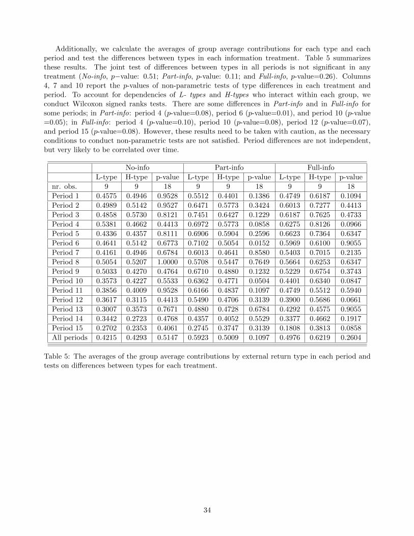
Additionally, we calculate the averages of group average contributions for each type and eachperiod and test the differences between types in each information treatment. Table 5 summarizesthese results. The joint test of differences between types in all periods is not significant in anytreatment (No-info, p−value: 0.51; Part-info, p-value: 0.11; and Full-info, p-value=0.26). Columns4, 7 and 10 report the p-values of non-parametric tests of type differences in each treatment andperiod. To account for dependencies of L- types and H-types who interact within each group, weconduct Wilcoxon signed ranks tests. There are some differences in Part-info and in Full-info forsome periods; in Part-info: period 4 (p-value=0.08), period 6 (p-value=0.01), and period 10 (p-value=0.05); in Full-info: period 4 (p-value=0.10), period 10 (p-value=0.08), period 12 (p-value=0.07),and period 15 (p-value=0.08). However, these results need to be taken with caution, as the necessaryconditions to conduct non-parametric tests are not satisfied. Period differences are not independent,but very likely to be correlated over time.

No-info Part-info Full-info

L-type H-type p-value L-type H-type p-value L-type H-type p-value

nr. obs. 9 9 18 9 9 18 9 9 18

Period 1 0.4575 0.4946 0.9528 0.5512 0.4401 0.1386 0.4749 0.6187 0.1094

Period 2 0.4989 0.5142 0.9527 0.6471 0.5773 0.3424 0.6013 0.7277 0.4413

Period 3 0.4858 0.5730 0.8121 0.7451 0.6427 0.1229 0.6187 0.7625 0.4733

Period 4 0.5381 0.4662 0.4413 0.6972 0.5773 0.0858 0.6275 0.8126 0.0966

Period 5 0.4336 0.4357 0.8111 0.6906 0.5904 0.2596 0.6623 0.7364 0.6347

Period 6 0.4641 0.5142 0.6773 0.7102 0.5054 0.0152 0.5969 0.6100 0.9055

Period 7 0.4161 0.4946 0.6784 0.6013 0.4641 0.8580 0.5403 0.7015 0.2135

Period 8 0.5054 0.5207 1.0000 0.5708 0.5447 0.7649 0.5664 0.6253 0.6347

Period 9 0.5033 0.4270 0.4764 0.6710 0.4880 0.1232 0.5229 0.6754 0.3743

Period 10 0.3573 0.4227 0.5533 0.6362 0.4771 0.0504 0.4401 0.6340 0.0847

Period 11 0.3856 0.4009 0.9528 0.6166 0.4837 0.1097 0.4749 0.5512 0.5940

Period 12 0.3617 0.3115 0.4413 0.5490 0.4706 0.3139 0.3900 0.5686 0.0661

Period 13 0.3007 0.3573 0.7671 0.4880 0.4728 0.6784 0.4292 0.4575 0.9055

Period 14 0.3442 0.2723 0.4768 0.4357 0.4052 0.5529 0.3377 0.4662 0.1917

Period 15 0.2702 0.2353 0.4061 0.2745 0.3747 0.3139 0.1808 0.3813 0.0858

All periods 0.4215 0.4293 0.5147 0.5923 0.5009 0.1097 0.4976 0.6219 0.2604

Table 5: The averages of the group average contributions by external return type in each period andtests on differences between types for each treatment.

34

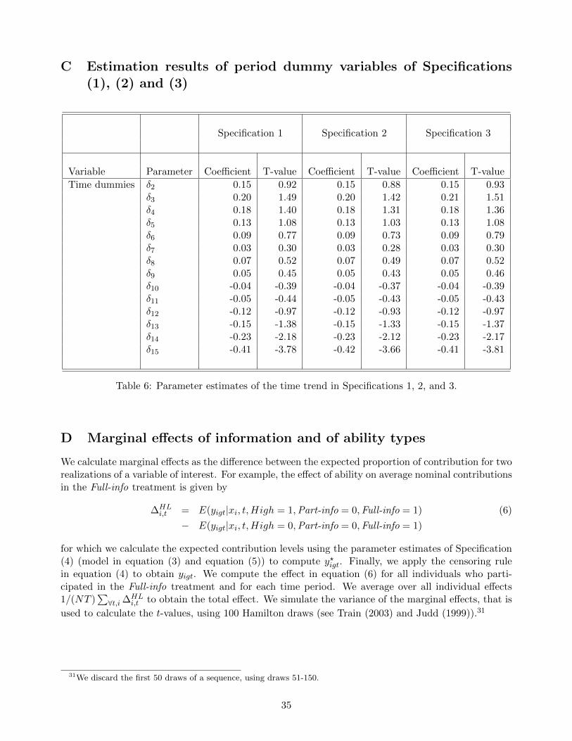
C Estimation results of period dummy variables of Specifications(1), (2) and (3)

Specification 1 Specification 2 Specification 3

Variable Parameter Coefficient T-value Coefficient T-value Coefficient T-value

Time dummies δ2 0.15 0.92 0.15 0.88 0.15 0.93δ3 0.20 1.49 0.20 1.42 0.21 1.51δ4 0.18 1.40 0.18 1.31 0.18 1.36δ5 0.13 1.08 0.13 1.03 0.13 1.08δ6 0.09 0.77 0.09 0.73 0.09 0.79δ7 0.03 0.30 0.03 0.28 0.03 0.30δ8 0.07 0.52 0.07 0.49 0.07 0.52δ9 0.05 0.45 0.05 0.43 0.05 0.46δ10 -0.04 -0.39 -0.04 -0.37 -0.04 -0.39δ11 -0.05 -0.44 -0.05 -0.43 -0.05 -0.43δ12 -0.12 -0.97 -0.12 -0.93 -0.12 -0.97δ13 -0.15 -1.38 -0.15 -1.33 -0.15 -1.37δ14 -0.23 -2.18 -0.23 -2.12 -0.23 -2.17δ15 -0.41 -3.78 -0.42 -3.66 -0.41 -3.81

Table 6: Parameter estimates of the time trend in Specifications 1, 2, and 3.

D Marginal effects of information and of ability types

We calculate marginal effects as the difference between the expected proportion of contribution for tworealizations of a variable of interest. For example, the effect of ability on average nominal contributionsin the Full-info treatment is given by

∆HLi,t = E(yigt|xi, t,High = 1,Part-info = 0,Full-info = 1) (6)

− E(yigt|xi, t,High = 0,Part-info = 0,Full-info = 1)

for which we calculate the expected contribution levels using the parameter estimates of Specification(4) (model in equation (3) and equation (5)) to compute y?igt. Finally, we apply the censoring rulein equation (4) to obtain yigt. We compute the effect in equation (6) for all individuals who parti-cipated in the Full-info treatment and for each time period. We average over all individual effects1/(NT )

∑∀t,i ∆HL

i,t to obtain the total effect. We simulate the variance of the marginal effects, that is

used to calculate the t-values, using 100 Hamilton draws (see Train (2003) and Judd (1999)).31

31We discard the first 50 draws of a sequence, using draws 51-150.

35

E Replication of Figures 2 and 3 based on Specification (3)

The two figures below replicate the marginal effects analysis of Figures 2 and 3 for Specification (3).Whereas average contributions are relatively well captured by Specification (3), the predicted marginaleffects based on Specification (3) do not capture very well the non-linearity present in the empiricaldifferences between types as shown in Figures 6 and 7 in F.

No-info, High No-info, Low

0 5 10 150.00.10.20.30.40.50.60.70.80.91.0

No-info, High No-info, Low Part-info, High Part-info, Low

0 5 10 150.00.10.20.30.40.50.60.70.80.91.0

Part-info, High Part-info, Low Full-info, High Full-info, Low

0 5 10 150.00.10.20.30.40.50.60.70.80.91.0

Full-info, High Full-info, Low

No-info

0 5 10 15-0.25

-0.15

-0.05

0.05

0.15

0.25No-info Part-info

0 5 10 15-0.25

-0.15

-0.05

0.05

0.15

0.25Part-info Full-info

0 5 10 15-0.25

-0.15

-0.05

0.05

0.15

0.25Full-info

Figure 4: Upper panels: Predicted average contributions (as a share of the endowment) over time foreach treatment and type.Lower panels: Marginal effects of external return types on contributions for each treatment. (Thegraphs project the difference in relative nominal contributions between H -types and L-types with 95%confidence bounds.)

High: Part vs. No-info

0 5 10 15-0.25

0.00

0.25 High: Part vs. No-info High: Full vs. No-info

0 5 10 15-0.25

0.00

0.25 High: Full vs. No-info High: Full vs. Part-info

0 5 10 15-0.25

0.00

0.25 High: Full vs. Part-info

Low: Part vs. No-info

0 5 10 15-0.25

0.00

0.25Low: Part vs. No-info Low: Full vs. No-info

0 5 10 15-0.25

0.00

0.25Low: Full vs. No-info Low: Full vs. Part-info

0 5 10 15-0.25

0.00

0.25Low: Full vs. Part-info

Figure 5: Marginal effects of information on contributions separately for H -types and L-types. (Thegraphs project the difference in relative nominal contributions between two information scenarios with95% confidence bounds.

36

F Replication of Figures 2 and 3 with empirical data

The two figures below (6 and 7) present average group contributions separately by type and informationtreatments as well as differences between these treatment groups and types over time. Thus theyreplicate with empirical data the marginal effects predictions of Figures 2 and 3 in the text (p. 22 andp. 24), and 4 and 5 in E.

.2.4

.6.8

0 5 10 15 0 5 10 15 0 5 10 15

No-info Part-info Full-info

Low High

Av. c

ontr.

as

% o

f w

Period

-.20

.2.4

0 5 10 15 0 5 10 15 0 5 10 15

No-info Part-info Full-info

Difference 95% confidence bounds

Dis

tanc

e H

-L in

% o

f w

Period

Figure 2 replicated with observed group averages

Figure 6: Observed average contributions (as a share of the endowment) over time for each treatmentand type (top panels) and differences between types (bottom panels) with 95% confidence bounds.

-.3-.2

-.10

.1.2

.3-.3

-.2-.1

0.1

.2.3

0 5 10 15

High

Low

Difference

95% conf.bounds

Diff

eren

ce(P

art-N

o-In

fo) i

n %

of w

Period

-.3-.2

-.10

.1.2

.3-.3

-.2-.1

0.1

.2.3

0 5 10 15

High

Low

Difference

95% conf.bounds

Diff

eren

ce(F

ull-N

o-In

fo) i

n %

of w

Period

-.3-.2

-.10

.1.2

.3-.3

-.2-.1

0.1

.2.3

0 5 10 15

High

Low

Difference

95% conf.bounds

Diff

eren

ce(F

ull-P

art-I

nfo)

in %

of w

Period

Figure 3 replicated with observed group averages

Figure 7: Observed differences in average contributions (as share of the endowment) separately forH -types and L-types. (The graphs project the difference in relative nominal contributions betweentwo information scenarios with 95% confidence bounds.)

37