
Public economics for development - UNU-WIDER · grateful to Jose Anchorena, Diego Schleser, Daniela...
36
DRAFT This is a draft version of a conference paper submitted for presentation at UNU-WIDER’s conference, held in Maputo on 5-6 July 2017. This is not a formal publication of UNU-WIDER and may reflect work-in-progress. Public economics for development 5-6 July 2017 | Maputo, Mozambique THIS DRAFT IS NOT TO BE CITED, QUOTED OR ATTRIBUTED WITHOUT PERMISSION FROM AUTHOR(S). WIDER Development Conference
-
Upload
nguyenthien -
Category
Documents
-
view
216 -
download
0
Transcript of Public economics for development - UNU-WIDER · grateful to Jose Anchorena, Diego Schleser, Daniela...

DRAFT
This is a draft version of a conference paper submitted for presentation at UNU-WIDER’s conference, held in Maputo on 5-6 July 2017. This is not a formal publication of UNU-WIDER and may refl ect work-in-progress.
Public economics for development5-6 July 2017 | Maputo, Mozambique
THIS DRAFT IS NOT TO BE CITED, QUOTED OR ATTRIBUTED WITHOUT PERMISSION FROM AUTHOR(S).
WIDER Development Conference
The Response of Salaried Workers to the Personal Income Tax:
Evidence from a Regression Discontinuity Design in Argentina ∗†
Santiago AfonsoMinistry of Treasury
Guillermo CrucesCEDLAS-UNLP, IZA
Victoria CastilloMTEySS
Dario TortaroloUC Berkeley
Abstract
This paper exploits a novel natural experiment to identify labor supply responsesto the personal income tax. In August 2013, the President of Argentina passed anExecutive Order that exempted from the income tax all wage earners with grossmonthly earnings between January and August 2013 below $AR 15,000, regardlessof subsequent earnings. This resulted in a large and salient discontinuity in taxliabilities for upper earning workers above and below 15k that were otherwise verysimilar. Using a regression discontinuity design and administrative employer-employeedata, we estimate a precisely measured zero change in earnings of salaried workers afterthe reform. Being more internally valid, this result challenges previous estimates ofreported income elasticities and the response of wage earners to tax cuts.
1 Introduction
The response of wage earners to taxes and tax reforms has long been of interest to economists
and policymakers. The magnitude of this response is of critical importance in the formulation
of tax and transfer policies, and for welfare analysis. However, the empirical literature has
not yet reached a consensus on the magnitude of the elasticity of earnings with respect to
∗We would like to thank Emmanuel Saez, Pat Kline, David Card, Hilary Hoynes, Alex Gelber, DannyYagan, Alan Auerbach, and Enrico Moretti for very helpful comments and discussions. We are especiallygrateful to Jose Anchorena, Diego Schleser, Daniela Guariniello, Moira Ohaco from the MTEySS of Argentinafor granting us access to the data and processing the codes making this work possible. The views expressedare those of the authors alone and do not necessarily reflect the views of the MTEySS.†Santiago Afonso, Ministry of Treasury and Public Finance, Buenos Aires, Argentina; Victoria Castillo,
Ministry of Labor, Employment, and Social Security, Buenos Aires, Argentina; Guillermo Cruces, CEDLAS- Universidad Nacional de La Plata, Argentina; Corresponding author: Dario Tortarolo, Department ofEconomics, UC Berkeley, 522 Evans Hall, Berkeley, CA. Email: [email protected]
1
tax rates. The empirical estimates are not fully compelling and range from no effect to very
sizeable responses.
In this article, we exploit a unique natural experiment that took place in Argentina in
the year 2013 to estimate earnings supply responses of salaried workers to the personal
income tax which overcomes identification difficulties that have plagued previous work.
Argentina has a progressive income tax schedule with seven brackets that has been fixed in
nominal terms since the year 2000. During this period, the country suffered an accumulated
inflation of approximately 1385% and nominal wages followed inflation over time. As a
result, a lot of people started paying the income tax in the last 15 years, and the system
lost a lot of progressivity since inflation reduced the significance of taxable thresholds.1 To
alleviate the increasing tax burden on wage earners, the president implemented in 2013
a permanent and large tax break for a group of workers based on prior earnings. This
unexpected reform was announced through an Executive Order in August 2013 and had the
following features: (i) wage earners whose highest gross monthly salary accrued between
January-August 2013 was below AR$ 15,000 were fully exempt from the income tax starting
in September 2013, regardless of subsequent earnings; (ii) wage earners whose highest gross
monthly salary accrued between January-August 2013 was between AR$ 15,001 and AR$
25,000 received a 20% increase in personal exemptions; (iii) workers earning +AR$ 25,001
between January-August 2013 continued paying the income tax normally. This tax break
was repealed by the new administration in February 2016.
As a result, in September 2013, about 1.5 million of wage earners suddenly stopped
paying the income tax regardless of subsequent earnings for two and a half years. This
reform implied that very similar workers ended up with very different tax liabilities from
September 2013 onwards, depending on whether their earnings from January to August
2013 were above or below 15k or 25k. Thus, the reform effectively created groups of workers
who coexist in the same labor market but face sharply different tax liabilities. Comparing
workers below and above these cutoffs using a regression discontinuity (RD) design offers a
unique opportunity to estimate the impact of a large and salient tax cut on earnings and
labor supply. We use administrative employer-employee data provided by the Ministry of
Labor, Employment and Social Security, the labor agency in Argentina. The data include
all private and public wage earners registered in the social security of Argentina.
Three main results are presented in the analysis. First, the first stage shows a large
discontinuity in tax liabilities for upper earning workers above and below 15k after the
reform. Second, we show that there is no discontinuity in the distribution of gross earnings
1In a companion paper we estimate the elasticity of earnings supply in Argentina using the “bracket creep”design by Saez (2003) as a natural experiment. The idea of bracket creep is that a taxpayer near the top-endof a bracket is likely to creep to the next bracket even if her income did not change in real terms.
2
between January and August 2013 around 15k or 25k. This suggests that individuals could
not game the law by underreporting earnings after the law was enacted to take advantage of
the tax break. This finding is crucial for the validity of the subsequent RD analysis. Third,
we find no evidence of earning responses to the tax cut along the intensive margin. Many
robustness checks confirm this result. Anecdotal evidence suggests that the reform and its
implementation were indeed very salient. The zero response of wage earners strikes us as
remarkable given the size and saliency of the tax cut. This finding could imply low efficiency
costs of income taxes for upper wage earners.
This paper complements a large empirical literature estimating the responses of reported
income to the personal income tax (see Saez, Slemrod, and Giertz 2012a for a recent
survey). Most of the existing work in this literature, however, is based on developed
countries. This paper, therefore, represents an effort at analyzing tax-driven responses of
wage earners in a developing country context. Moreover, a variety of estimation methods
have been employed, including difference-in-differences based on repeated cross sections,
share analysis, panel-based difference-in-differences, and instrumental variables. But none
of them used a regression discontinuity design, as we do, which is known to have stronger
internal validity. Finally, this paper is also connected to a recent strand of literature that
has challenged conventional wisdom by finding precisely measured zero effects of different
taxes on economic outcomes. For example, using a cohort-based reform in Greece, Saez,
Matsaganis, and Tsakloglou (2012b) find no responses of labor supply to payroll taxes along
the extensive and intensive margins around a discontinuity, suggesting low efficiency costs
of payroll taxes. Bastani and Selin (2014) obtain a precise zero response of wage earners to
a large kink point of the Swedish tax schedule using the bunching method. In a different
context, Yagan (2015) estimates that the 2003 dividend tax cut in the U.S. caused zero
change in corporate investment and employee compensation. This paper contributes to this
literature by documenting that in contrast to numerous other tax reforms studied, a large
and salient tax cut had no detectable near-term impact on the earnings of salaried workers.
The article is organized as follows. Section 2 describes the institutional details and the
conceptual framework. Section 3 introduces the administrative data and summary statistics.
Section 4 presents the empirical strategy and results. Section 5 concludes.
3
2 Institutional Setting and Conceptual Framework
2.1 Overview of the Argentine tax system
Argentina levies taxes at the federal, provincial, and municipal level. The federal tax system
is based on the following main taxes: corporate and personal income tax, payroll tax, value
added tax, import and export taxes, tax on financial transactions, and net worth tax. The
fiscal pressure (total revenue/GDP) has increased substantially in the last years, from 20%
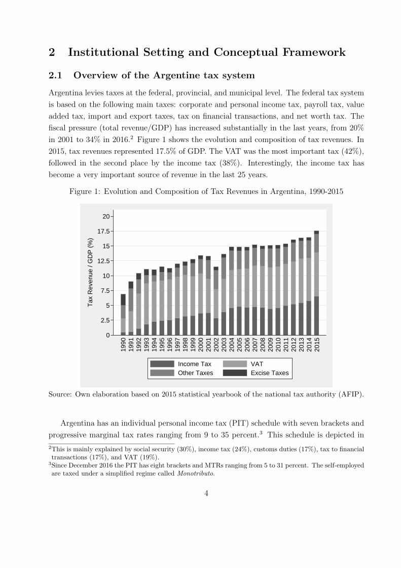
in 2001 to 34% in 2016.2 Figure 1 shows the evolution and composition of tax revenues. In
2015, tax revenues represented 17.5% of GDP. The VAT was the most important tax (42%),
followed in the second place by the income tax (38%). Interestingly, the income tax has
become a very important source of revenue in the last 25 years.
Figure 1: Evolution and Composition of Tax Revenues in Argentina, 1990-2015
0
2.5
5
7.5
10
12.5
15
17.5
20
Tax
Rev
enue
/ G
DP
(%
)
1990
1991
1992
1993
1994
1995
1996
1997
1998
1999
2000
2001
2002
2003
2004
2005
2006
2007
2008
2009
2010
2011
2012
2013
2014
2015
Income Tax VATOther Taxes Excise Taxes
Source: Own elaboration based on 2015 statistical yearbook of the national tax authority (AFIP).
Argentina has an individual personal income tax (PIT) schedule with seven brackets and
progressive marginal tax rates ranging from 9 to 35 percent.3 This schedule is depicted in
2This is mainly explained by social security (30%), income tax (24%), customs duties (17%), tax to financialtransactions (17%), and VAT (19%).
3Since December 2016 the PIT has eight brackets and MTRs ranging from 5 to 31 percent. The self-employedare taxed under a simplified regime called Monotributo.
4
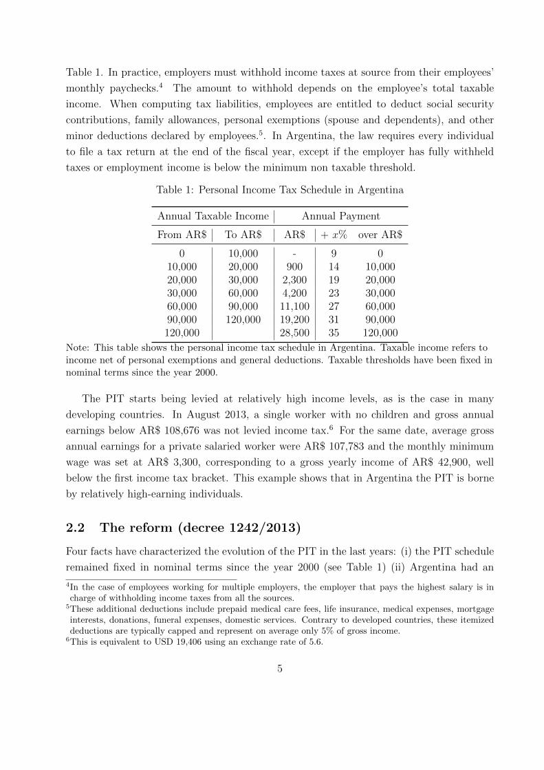
Table 1. In practice, employers must withhold income taxes at source from their employees’
monthly paychecks.4 The amount to withhold depends on the employee’s total taxable
income. When computing tax liabilities, employees are entitled to deduct social security
contributions, family allowances, personal exemptions (spouse and dependents), and other
minor deductions declared by employees.5. In Argentina, the law requires every individual
to file a tax return at the end of the fiscal year, except if the employer has fully withheld
taxes or employment income is below the minimum non taxable threshold.
Table 1: Personal Income Tax Schedule in Argentina
Annual Taxable Income Annual Payment
From AR$ To AR$ AR$ + x% over AR$
0 10,000 - 9 010,000 20,000 900 14 10,00020,000 30,000 2,300 19 20,00030,000 60,000 4,200 23 30,00060,000 90,000 11,100 27 60,00090,000 120,000 19,200 31 90,000120,000 28,500 35 120,000
Note: This table shows the personal income tax schedule in Argentina. Taxable income refers toincome net of personal exemptions and general deductions. Taxable thresholds have been fixed innominal terms since the year 2000.
The PIT starts being levied at relatively high income levels, as is the case in many
developing countries. In August 2013, a single worker with no children and gross annual
earnings below AR$ 108,676 was not levied income tax.6 For the same date, average gross
annual earnings for a private salaried worker were AR$ 107,783 and the monthly minimum
wage was set at AR$ 3,300, corresponding to a gross yearly income of AR$ 42,900, well
below the first income tax bracket. This example shows that in Argentina the PIT is borne
by relatively high-earning individuals.
2.2 The reform (decree 1242/2013)
Four facts have characterized the evolution of the PIT in the last years: (i) the PIT schedule
remained fixed in nominal terms since the year 2000 (see Table 1) (ii) Argentina had an
4In the case of employees working for multiple employers, the employer that pays the highest salary is incharge of withholding income taxes from all the sources.
5These additional deductions include prepaid medical care fees, life insurance, medical expenses, mortgageinterests, donations, funeral expenses, domestic services. Contrary to developed countries, these itemizeddeductions are typically capped and represent on average only 5% of gross income.
6This is equivalent to USD 19,406 using an exchange rate of 5.6.
5
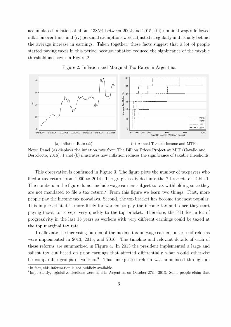
accumulated inflation of about 1385% between 2002 and 2015; (iii) nominal wages followed
inflation over time; and (iv) personal exemptions were adjusted irregularly and usually behind
the average increase in earnings. Taken together, these facts suggest that a lot of people
started paying taxes in this period because inflation reduced the significance of the taxable
threshold as shown in Figure 2.
Figure 2: Inflation and Marginal Tax Rates in Argentina
0
10
20
30
40
%
1/1/2004 1/1/2006 1/1/2008 1/1/2010 1/1/2012 1/1/2014 1/1/2016
(a) Inflation Rate (%)
9
14
19
23
27
31
35
Mar
gina
l Tax
Rat
es (%
)
0 10k 20k 30k 60k 90k 120kTaxable Income (2003 AR pesos)
2003200720112014
(b) Annual Taxable Income and MTRs
Note: Panel (a) displays the inflation rate from The Billion Prices Project at MIT (Cavallo andBertolotto, 2016). Panel (b) illustrates how inflation reduces the significance of taxable thresholds.
This observation is confirmed in Figure 3. The figure plots the number of taxpayers who
filed a tax return from 2000 to 2014. The graph is divided into the 7 brackets of Table 1.
The numbers in the figure do not include wage earners subject to tax withholding since they
are not mandated to file a tax return.7 From this figure we learn two things. First, more
people pay the income tax nowadays. Second, the top bracket has become the most popular.
This implies that it is more likely for workers to pay the income tax and, once they start
paying taxes, to “creep” very quickly to the top bracket. Therefore, the PIT lost a lot of
progressivity in the last 15 years as workers with very different earnings could be taxed at
the top marginal tax rate.
To alleviate the increasing burden of the income tax on wage earners, a series of reforms
were implemented in 2013, 2015, and 2016. The timeline and relevant details of each of
these reforms are summarized in Figure 4. In 2013 the president implemented a large and
salient tax cut based on prior earnings that affected differentially what would otherwise
be comparable groups of workers.8 This unexpected reform was announced through an
7In fact, this information is not publicly available.8Importantly, legislative elections were held in Argentina on October 27th, 2013. Some people claim that
6
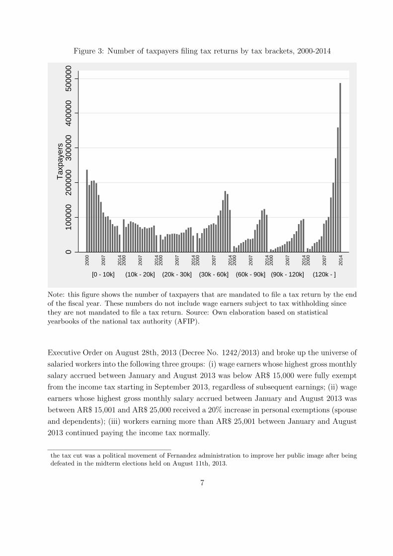
Figure 3: Number of taxpayers filing tax returns by tax brackets, 2000-2014
010
0000
2000
0030
0000
4000
0050
0000
Tax
paye
rs
[0 - 10k] (10k - 20k] (20k - 30k] (30k - 60k] (60k - 90k] (90k - 120k] (120k - ]
2000
20
07
2014
2000
20
07
2014
2000
20
07
2014
2000
20
07
2014
2000
20
07
2014
2000
20
07
2014
2000
20
07
2014
Note: this figure shows the number of taxpayers that are mandated to file a tax return by the endof the fiscal year. These numbers do not include wage earners subject to tax withholding sincethey are not mandated to file a tax return. Source: Own elaboration based on statisticalyearbooks of the national tax authority (AFIP).
Executive Order on August 28th, 2013 (Decree No. 1242/2013) and broke up the universe of
salaried workers into the following three groups: (i) wage earners whose highest gross monthly
salary accrued between January and August 2013 was below AR$ 15,000 were fully exempt
from the income tax starting in September 2013, regardless of subsequent earnings; (ii) wage
earners whose highest gross monthly salary accrued between January and August 2013 was
between AR$ 15,001 and AR$ 25,000 received a 20% increase in personal exemptions (spouse
and dependents); (iii) workers earning more than AR$ 25,001 between January and August
2013 continued paying the income tax normally.
the tax cut was a political movement of Fernandez administration to improve her public image after beingdefeated in the midterm elections held on August 11th, 2013.
7
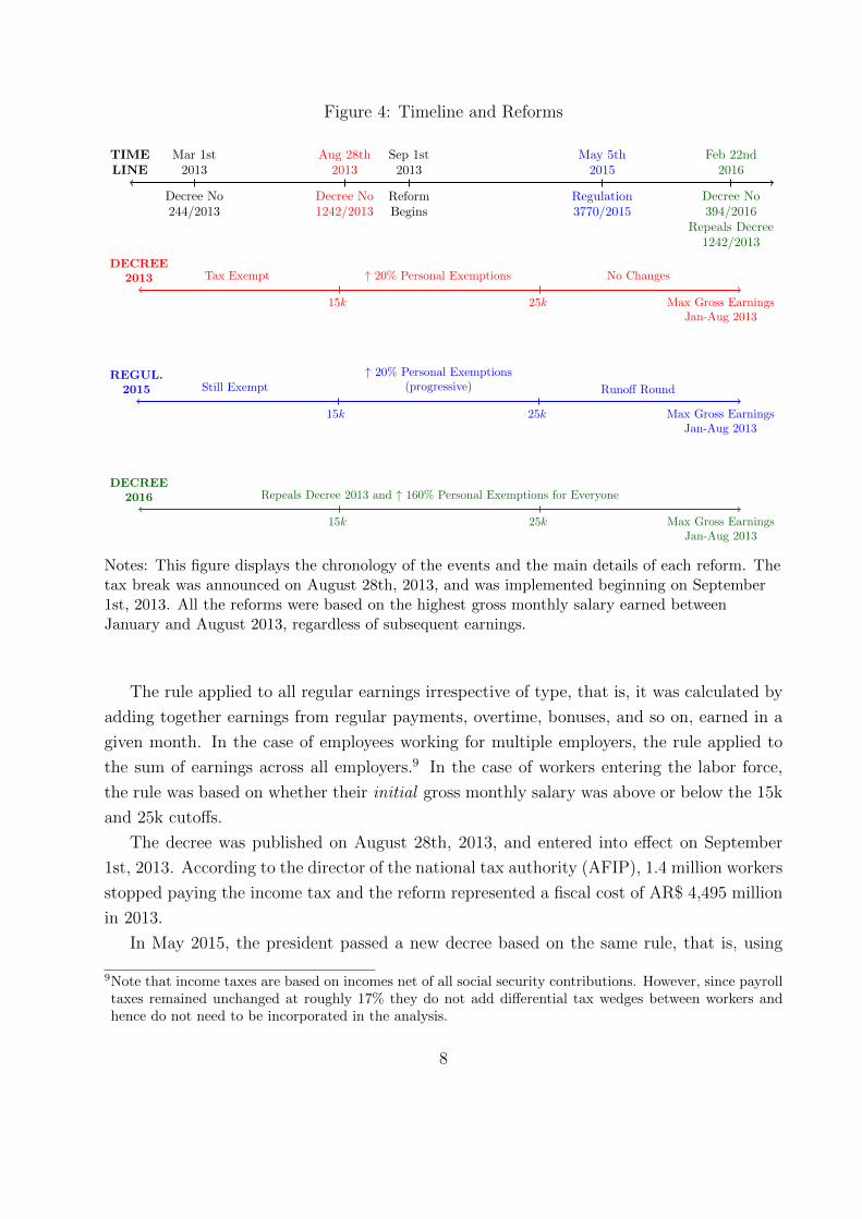
Figure 4: Timeline and Reforms
TIMELINE
Decree No244/2013
Mar 1st2013
Decree No1242/2013
Aug 28th2013
ReformBegins
Sep 1st2013
Regulation3770/2015
May 5th2015
Decree No394/2016
Repeals Decree1242/2013
Feb 22nd2016
DECREE2013 Tax Exempt
15k
↑ 20% Personal Exemptions
25k
No Changes
Max Gross EarningsJan-Aug 2013
REGUL.2015 Still Exempt
15k
↑ 20% Personal Exemptions(progressive)
25k
Runoff Round
Max Gross EarningsJan-Aug 2013
DECREE2016
15k
Repeals Decree 2013 and ↑ 160% Personal Exemptions for Everyone
25k Max Gross EarningsJan-Aug 2013
1
Notes: This figure displays the chronology of the events and the main details of each reform. Thetax break was announced on August 28th, 2013, and was implemented beginning on September1st, 2013. All the reforms were based on the highest gross monthly salary earned betweenJanuary and August 2013, regardless of subsequent earnings.
The rule applied to all regular earnings irrespective of type, that is, it was calculated by
adding together earnings from regular payments, overtime, bonuses, and so on, earned in a
given month. In the case of employees working for multiple employers, the rule applied to
the sum of earnings across all employers.9 In the case of workers entering the labor force,
the rule was based on whether their initial gross monthly salary was above or below the 15k
and 25k cutoffs.
The decree was published on August 28th, 2013, and entered into effect on September
1st, 2013. According to the director of the national tax authority (AFIP), 1.4 million workers
stopped paying the income tax and the reform represented a fiscal cost of AR$ 4,495 million
in 2013.
In May 2015, the president passed a new decree based on the same rule, that is, using
9Note that income taxes are based on incomes net of all social security contributions. However, since payrolltaxes remained unchanged at roughly 17% they do not add differential tax wedges between workers andhence do not need to be incorporated in the analysis.
8
the highest monthly earnings accrued between January and August 2013. In this case, the
decree only increased personal exemptions by 20% for the group of workers with earnings
between 15k and 25k. Finally, in February 2016 the new administration put an end to the
tax break and increased personal exemptions for everyone by 160%.
The reform of 2013 implied that very similar workers ended up with very different tax
liabilities from September 2013 onwards, depending on whether their earnings from January
to August 2013 were above or below 15k or 25k. Comparing workers below and above these
cutoffs using a regression discontinuity design offers a unique opportunity to estimate the
impact of a large and salient tax cut on earnings and labor supply.
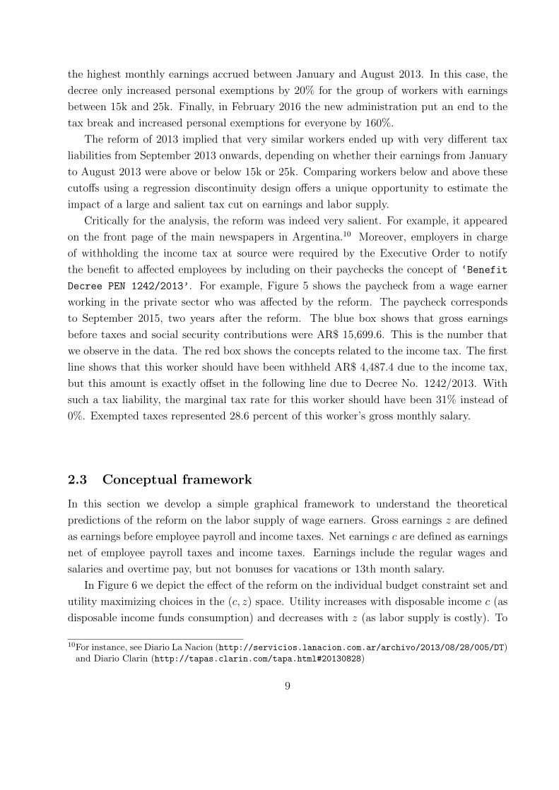
Critically for the analysis, the reform was indeed very salient. For example, it appeared
on the front page of the main newspapers in Argentina.10 Moreover, employers in charge
of withholding the income tax at source were required by the Executive Order to notify
the benefit to affected employees by including on their paychecks the concept of ‘Benefit
Decree PEN 1242/2013’. For example, Figure 5 shows the paycheck from a wage earner
working in the private sector who was affected by the reform. The paycheck corresponds
to September 2015, two years after the reform. The blue box shows that gross earnings
before taxes and social security contributions were AR$ 15,699.6. This is the number that
we observe in the data. The red box shows the concepts related to the income tax. The first
line shows that this worker should have been withheld AR$ 4,487.4 due to the income tax,
but this amount is exactly offset in the following line due to Decree No. 1242/2013. With
such a tax liability, the marginal tax rate for this worker should have been 31% instead of
0%. Exempted taxes represented 28.6 percent of this worker’s gross monthly salary.
2.3 Conceptual framework
In this section we develop a simple graphical framework to understand the theoretical
predictions of the reform on the labor supply of wage earners. Gross earnings z are defined
as earnings before employee payroll and income taxes. Net earnings c are defined as earnings
net of employee payroll taxes and income taxes. Earnings include the regular wages and
salaries and overtime pay, but not bonuses for vacations or 13th month salary.
In Figure 6 we depict the effect of the reform on the individual budget constraint set and
utility maximizing choices in the (c, z) space. Utility increases with disposable income c (as
disposable income funds consumption) and decreases with z (as labor supply is costly). To
10For instance, see Diario La Nacion (http://servicios.lanacion.com.ar/archivo/2013/08/28/005/DT)and Diario Clarin (http://tapas.clarin.com/tapa.html#20130828)
9
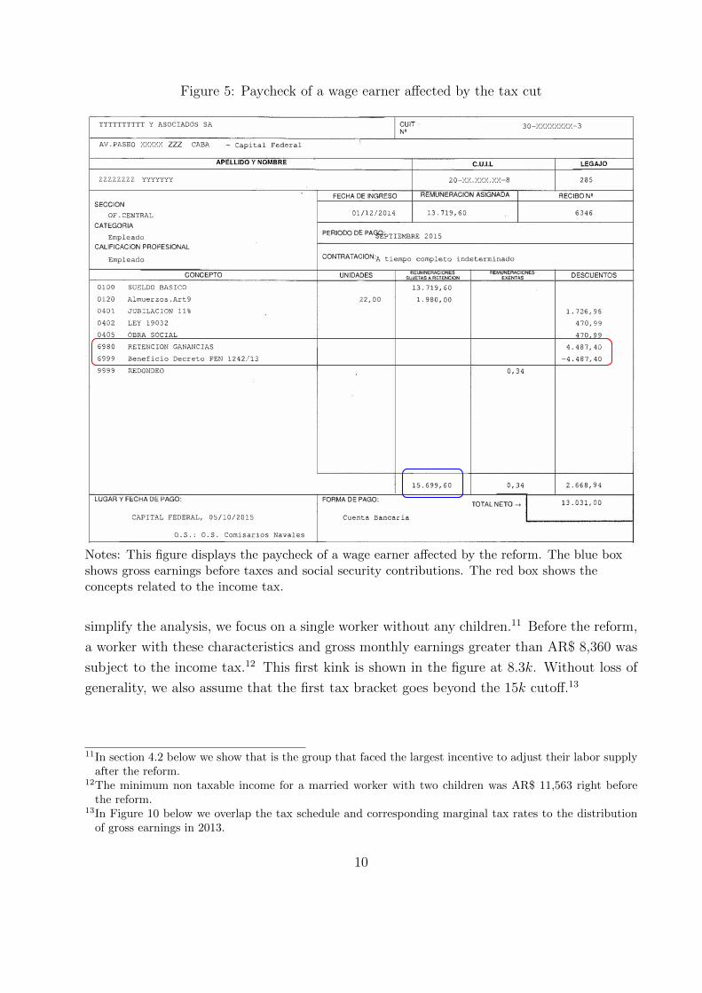
Figure 5: Paycheck of a wage earner affected by the tax cut
TTTTTTTTTT Y ASOCIADOS SA
AV. PASEO XXXXX ZZZ CABA Capital Federal
APELLIDO Y NOMBRE
ZZZZZZZZ YYYYYYY
SECCION
OF.CENTRAL
CATEGORIA
Empleado CALIFICACiON PROFESIONAL
Empleado
CONCEPTO
0100 SU:i'.:LDO BASICO
0.1.20 Almuerzos.Art9
0401. JOBI LAC ION 11%
0402 LEY 19032
0405 OBRA SOCIAL
6980 RETENCION GANANCIAS
6999 Beneficio Decreto PEN 1242/13
9999 REDON�EO
LUGAR Y FECHA DE PAGO:
CAPITAL FEDERAL, 05/10/2015
0. S.: o.s. Comisarios Navales
SON PESOS: Trece Mil Treinta y Uno
Los haberes ae depositaran en la cuenta :Nro.
ART. 12 LEY 17250
MES AGOSTO 2015
BANCO HSBC
FECHA DEPOSITO 24/09/2015
CUIT 30-XXXXXXXX-3N'
C.U.I.L
FECHA DE INGRESO
20-XX.XXX.XX-8
REMUNERACION ASIGNADA
01/12/2014 13.719,60
PERIODO DE PA�?TIEMBRE 2015
CONTRATACION:A tiempo completo indeterminado
UNIDADES REUMNERACIONES REMUNEAACIONES
SUJETAS A RETENCION EXENTAS
13' 719,60
22, 00 1.980,00
0,34
15.699,60 0,34
FORMA DE PAGO: TOTAL NETO--+
Cuenta Bancaria
3046054578 del Banco HSBC
--
LEGAJO
285
AECIBO N2
6346
DESCUENTOS
1.726,96
470,99
470,99
4.487,40
-4.487,40
2.668,94
13.031,00
(;{�t···
. ii,
.•• .
FIRMA DEL
-·--··-'"
PDF processed with CutePDF evaluation edition www.CutePDF.com
Notes: This figure displays the paycheck of a wage earner affected by the reform. The blue boxshows gross earnings before taxes and social security contributions. The red box shows theconcepts related to the income tax.
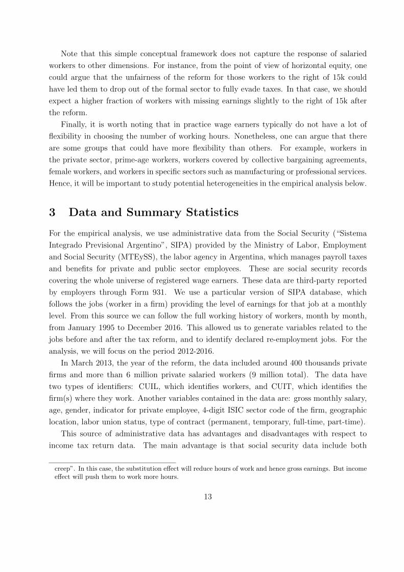
simplify the analysis, we focus on a single worker without any children.11 Before the reform,
a worker with these characteristics and gross monthly earnings greater than AR$ 8,360 was
subject to the income tax.12 This first kink is shown in the figure at 8.3k. Without loss of
generality, we also assume that the first tax bracket goes beyond the 15k cutoff.13
11In section 4.2 below we show that is the group that faced the largest incentive to adjust their labor supplyafter the reform.
12The minimum non taxable income for a married worker with two children was AR$ 11,563 right beforethe reform.
13In Figure 10 below we overlap the tax schedule and corresponding marginal tax rates to the distributionof gross earnings in 2013.
10
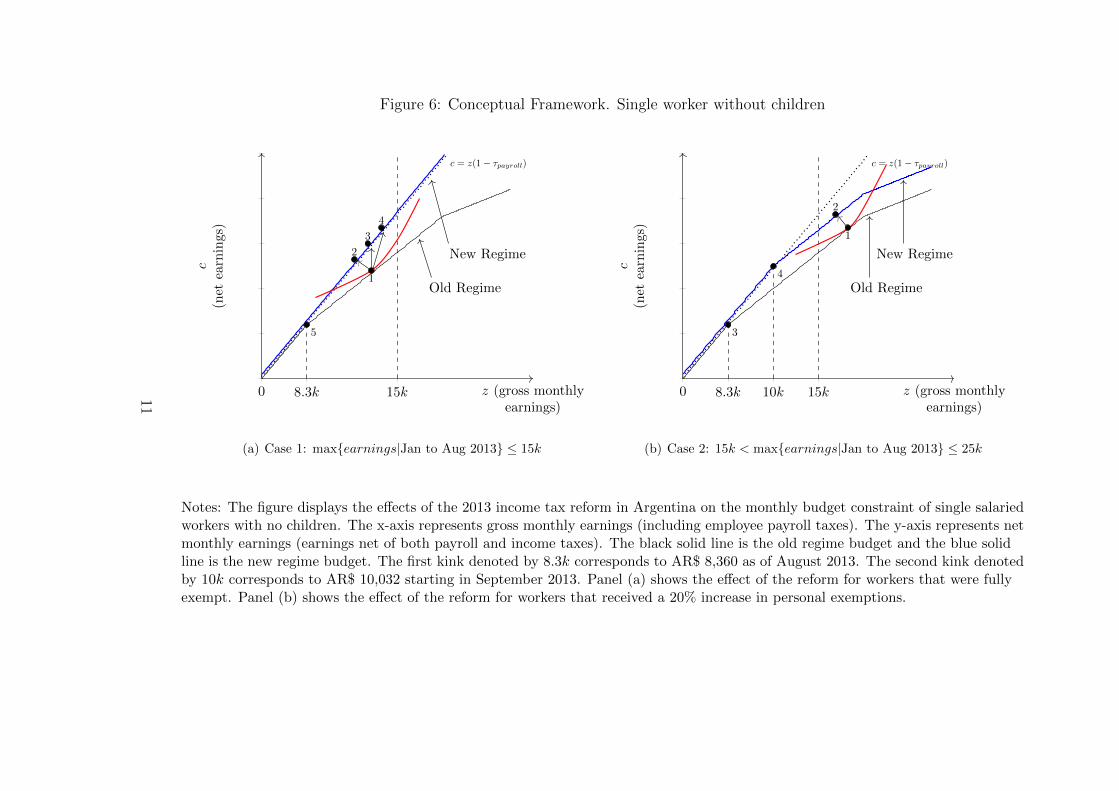
Figure 6: Conceptual Framework. Single worker without children
0 8.3k 15k
c = z(1− τpayroll)
New Regime
Old Regime1
2
3
4
5
z (gross monthlyearnings)
c(net
earnings)
(a) Case 1: max{earnings|Jan to Aug 2013} ≤ 15k
0 8.3k 10k 15k
c = z(1− τpayroll)
New Regime
Old Regime
1
2
3
4
z (gross monthlyearnings)
c(net
earnings)
(b) Case 2: 15k < max{earnings|Jan to Aug 2013} ≤ 25k
Notes: The figure displays the effects of the 2013 income tax reform in Argentina on the monthly budget constraint of single salariedworkers with no children. The x-axis represents gross monthly earnings (including employee payroll taxes). The y-axis represents netmonthly earnings (earnings net of both payroll and income taxes). The black solid line is the old regime budget and the blue solidline is the new regime budget. The first kink denoted by 8.3k corresponds to AR$ 8,360 as of August 2013. The second kink denotedby 10k corresponds to AR$ 10,032 starting in September 2013. Panel (a) shows the effect of the reform for workers that were fullyexempt. Panel (b) shows the effect of the reform for workers that received a 20% increase in personal exemptions.
11

Figure 6 panel (a) shows the predicted effects of the reform for individuals whose highest
gross monthly salary accrued between January and August 2013 was less than AR$ 15,000.
These wage earners were fully exempt from the income tax from September 2013 onwards,
regardless of subsequent earnings. Along the intensive margin, workers below 8.3k were not
paying income taxes before the reform and thus are unaffected. Workers with pre-reform
earnings between 8.3k and 15k experience a decrease in marginal income tax rates from
τ > 0 to τ = 0 so that their net-of-income-tax rate increases from 1− τ to 1. Their budget
set shifts upwards from the black solid line to the blue solid line. This creates substitution
and income effects.
The substitution effect pushes individuals to work more hours increasing gross earnings.
Intuitively, individuals have incentives to work more hours, accept promotions, or job offers
at a different place, because they can keep the full payment. However, holding everything
else constant, workers maximizing utility in z ∈ (8.3k, 15k] will get a higher take-home pay
now. Thus, the income effect pushes individuals to work less hours reducing gross earnings.
Hence, a worker maximizing utility at point 1 could end up in points like 2, 3, or 4. Thus,
the effect of the tax break on earnings for this group of workers is ambiguous. Finally,
note that workers bunching at the first kink 8.3k (i.e. maximizing at point 5) experience a
substitution effect that will push them to work more hours (or report higher earnings). This
implies that after the reform we should expect bunching at the first kink (if any) to decrease
substantially.
Figure 6 panel (b) shows the predicted effects of the reform for individuals whose highest
gross monthly salary accrued between January and August 2013 was between AR$ 15,001
and AR$ 25,000. In this case, the reform increased the minimum non taxable income 20%
from 8.3k to 10k, hence shifting outward the first kink point in the budget set.14 Workers
with pre-reform earnings between 15k and 25k experience no changes in marginal income
tax rates and therefore the substitution effect is zero. However, holding everything else
constant, workers maximizing utility in z ∈ (15k, 25k] will get a higher take-home pay now.
Thus, income effect reduces hours of work and hence gross earnings. For example, a worker
maximizing utility at point 1 would go to a point like 2. Finally, note that the first kink
moved from 8.3k to 10k (point 3 to 4). However, this change should not matter for the
analysis as, by definition, this group of workers were making more than 15k before the
reform.
Finally, workers whose highest gross monthly salary accrued between January and August
2013 was greater than AR$ 25,001 were not affected by the reform.15
14The 20% increase in personal exemptions corresponds to deductions for spouse, children, and a specialdeduction for wage earners.
15In fact, this group of workers experience an increase in average tax rates due to inflation and the “bracket
12
Note that this simple conceptual framework does not capture the response of salaried
workers to other dimensions. For instance, from the point of view of horizontal equity, one
could argue that the unfairness of the reform for those workers to the right of 15k could
have led them to drop out of the formal sector to fully evade taxes. In that case, we should
expect a higher fraction of workers with missing earnings slightly to the right of 15k after
the reform.
Finally, it is worth noting that in practice wage earners typically do not have a lot of
flexibility in choosing the number of working hours. Nonetheless, one can argue that there
are some groups that could have more flexibility than others. For example, workers in
the private sector, prime-age workers, workers covered by collective bargaining agreements,
female workers, and workers in specific sectors such as manufacturing or professional services.
Hence, it will be important to study potential heterogeneities in the empirical analysis below.
3 Data and Summary Statistics
For the empirical analysis, we use administrative data from the Social Security (“Sistema
Integrado Previsional Argentino”, SIPA) provided by the Ministry of Labor, Employment
and Social Security (MTEySS), the labor agency in Argentina, which manages payroll taxes
and benefits for private and public sector employees. These are social security records
covering the whole universe of registered wage earners. These data are third-party reported
by employers through Form 931. We use a particular version of SIPA database, which
follows the jobs (worker in a firm) providing the level of earnings for that job at a monthly
level. From this source we can follow the full working history of workers, month by month,
from January 1995 to December 2016. This allowed us to generate variables related to the
jobs before and after the tax reform, and to identify declared re-employment jobs. For the
analysis, we will focus on the period 2012-2016.
In March 2013, the year of the reform, the data included around 400 thousands private
firms and more than 6 million private salaried workers (9 million total). The data have
two types of identifiers: CUIL, which identifies workers, and CUIT, which identifies the
firm(s) where they work. Another variables contained in the data are: gross monthly salary,
age, gender, indicator for private employee, 4-digit ISIC sector code of the firm, geographic
location, labor union status, type of contract (permanent, temporary, full-time, part-time).
This source of administrative data has advantages and disadvantages with respect to
income tax return data. The main advantage is that social security data include both
creep”. In this case, the substitution effect will reduce hours of work and hence gross earnings. But incomeeffect will push them to work more hours.
13
workers paying the income tax and not paying the income tax. This feature is crucial for the
analysis which requires to follow workers that were fully exempt after the reform, and this
is the reason why we chose SIPA. Ideally, one would also want to observe the marital status
and number of dependents in every year and calculate the response of salaried workers for
single and married workers separately. Such administrative data are typically available in
income tax return data, but this is not the case for the SIPA database.16 Finally, it is worth
mentioning that in the SIPA database it is not possible to decompose the gross salary into
its different components such as bonuses, overtime pay, vacations, and 13th salary. Income
tax data typically allow to decompose taxable income into different margins.17
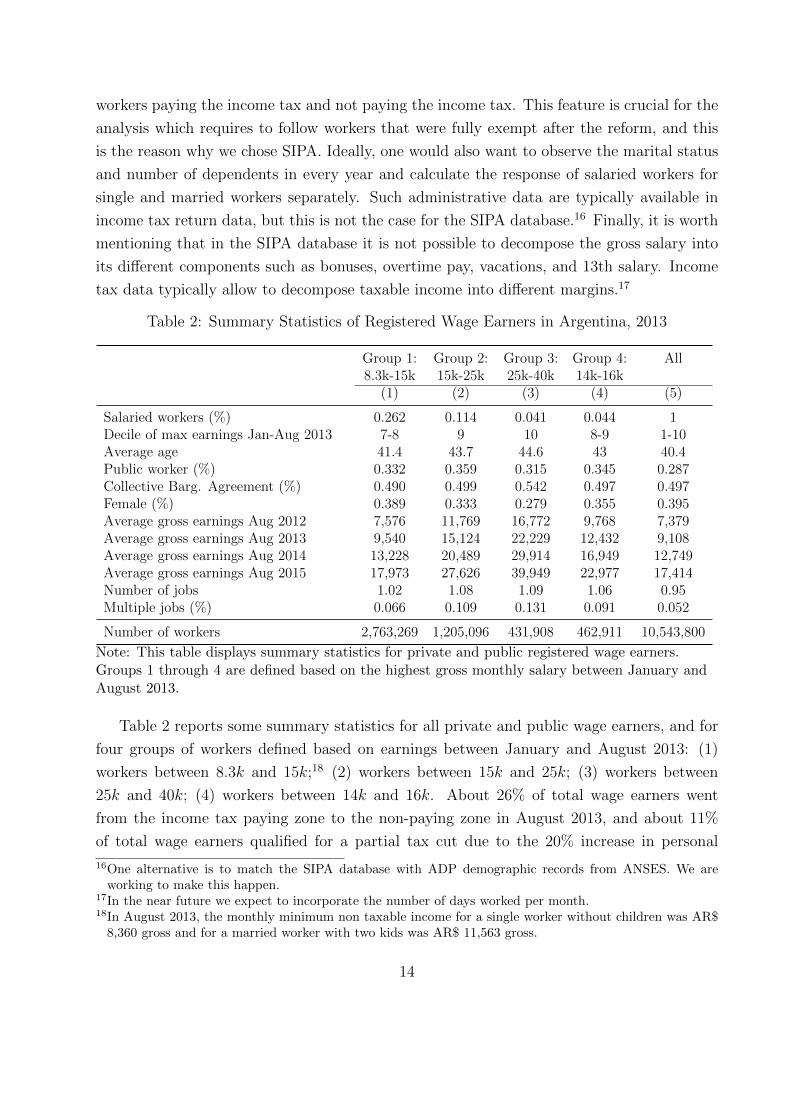
Table 2: Summary Statistics of Registered Wage Earners in Argentina, 2013
Group 1: Group 2: Group 3: Group 4: All8.3k-15k 15k-25k 25k-40k 14k-16k
(1) (2) (3) (4) (5)
Salaried workers (%) 0.262 0.114 0.041 0.044 1Decile of max earnings Jan-Aug 2013 7-8 9 10 8-9 1-10Average age 41.4 43.7 44.6 43 40.4Public worker (%) 0.332 0.359 0.315 0.345 0.287Collective Barg. Agreement (%) 0.490 0.499 0.542 0.497 0.497Female (%) 0.389 0.333 0.279 0.355 0.395Average gross earnings Aug 2012 7,576 11,769 16,772 9,768 7,379Average gross earnings Aug 2013 9,540 15,124 22,229 12,432 9,108Average gross earnings Aug 2014 13,228 20,489 29,914 16,949 12,749Average gross earnings Aug 2015 17,973 27,626 39,949 22,977 17,414Number of jobs 1.02 1.08 1.09 1.06 0.95Multiple jobs (%) 0.066 0.109 0.131 0.091 0.052
Number of workers 2,763,269 1,205,096 431,908 462,911 10,543,800
Note: This table displays summary statistics for private and public registered wage earners.Groups 1 through 4 are defined based on the highest gross monthly salary between January andAugust 2013.
Table 2 reports some summary statistics for all private and public wage earners, and for
four groups of workers defined based on earnings between January and August 2013: (1)
workers between 8.3k and 15k;18 (2) workers between 15k and 25k; (3) workers between
25k and 40k; (4) workers between 14k and 16k. About 26% of total wage earners went
from the income tax paying zone to the non-paying zone in August 2013, and about 11%
of total wage earners qualified for a partial tax cut due to the 20% increase in personal
16One alternative is to match the SIPA database with ADP demographic records from ANSES. We areworking to make this happen.
17In the near future we expect to incorporate the number of days worked per month.18In August 2013, the monthly minimum non taxable income for a single worker without children was AR$
8,360 gross and for a married worker with two kids was AR$ 11,563 gross.
14
exemptions.19 These two groups of workers belong to the 7th, 8th, and 9th deciles. Hence,
the reform studied mainly affected upper earning workers.
Narrowing the attention to the group of workers located around 15k, which is the main
discontinuity introduced by the reform, we can see that they are prime-age workers, 34%
work in the public sector, half of them are covered by a collective bargaining agreement,
35% are female workers, and around 9% have more than one job. It is worth noting that
in August 2013 average earnings for this group were AR$ 12,432, well below the cutoff that
determined who was exempt from that point onwards.
4 Empirical Strategy and Results
To analyze the response of individuals to the income tax, one could estimate a regression of
the change in reported income on the change in the net-of-tax rate. This regression is clearly
endogenous because the marginal tax rate is a function of taxable income.20 Hence, the
literature has typically relied on exogenous variation provided by tax reforms and a variety
of (imperfect) estimation techniques to identify the elasticity of income to taxes (see Saez et
al. 2012a for a recent survey). In this paper, we use a regression discontinuity design (RDD)
which is known to be more internally valid and thus overcomes identification difficulties that
have plagued previous work.
As the August 2013 reform was based on gross monthly earnings accrued between January
and August of that year, the strategy is to compare labor market outcomes after the reform
based on these earnings. The reform created a sharp discontinuity on tax liabilities depending
on whether wage earners were below or above the 15k and 25k cutoffs. This feature leads
naturally to a regression discontinuity design. The basic idea is to compare wage earners
just above and just below the thresholds (15k and 25k) to infer the causal effect of the tax
cut. This design is appealing because it is relatively simple and transparent. Therefore, we
will identify tax effects by running regressions of the form:
Yi = α + β · 1(Ri ≤ c) +K∑k=1
γ0k · (Ri − c)k +K∑k=1
γ1k · 1(Ri ≤ c)(Ri − c)k + ei (1)
where Yi denotes gross earnings for worker i in any month after the reform, Ri is the running
19In practice, the number of workers that effectively went from paying the income tax to being tax exemptis lower because personal deductions vary by marital status and number of dependents.
20Another two threats typically considered by the literature are mean reversion and heterogenous incometrend.
15
variable defined as
Ri ≡ max{Yi in January to August 2013} (2)
and c = 15k, 25k are the cutoffs of interest. The coefficient of interest capturing the effect
of the discontinuity at c = 15k is β. A simple way to illustrate the RD is to plot average
outcome Yi by disjoint bins of the running variable Ri and draw a polynomial fit below
and above the cutoffs. Intuitively, the treatment may be as good as randomly assigned for
individuals in the neighborhood of Ri = c, so comparing treated and non-treated workers
reveals a treatment effect (i.e. the effect of a large tax cut on earnings labor supply). The
outcomes considered in the analysis below include: average gross earnings, percentiles of
earnings, fraction of workers with multiple jobs, fraction of workers with missing earnings,
percentage change in gross earnings, probability that the increase in earnings is greater than
inflation.
4.1 Identification Checks
A fundamental RD identifying assumption is that 1(Ri ≤ c) must be as good as randomly
assigned in the neighborhood of Ri = c. This may be violated if individuals can exactly
control the value of Ri and therefore the location relative to the threshold. If individuals
are strategically locating above or below the threshold to benefit from the tax cut, we would
expect bunching on whichever side of the discontinuity is preferable (in this case the left
side).
Figure 7 presents a visual test for this threat. The figure plots the distribution of the
highest gross monthly salary between January and August 2013. Reassuringly, wage earners
did not sort in the neighborhood of the thresholds. Specifically, we observe no spike in the
number of wage earners just below 15k and 25k. Another important observation is that
wage earners do not seem to bunch at the first kink point of the income tax denoted by MNI
in the figure. The absence of bunching at the first kink already suggests that the overall
response of salaried workers to the income tax ought to be small in Argentina.21 However,
the earnings distribution does show bunching at 7k due to the family allowance program
(AA.FF.).22 This bunching suggests that wage earners do have some space or flexibility to
21This result is at odd with empirical findings in other countries such as the U.S. where Saez (2010) findsevidence of bunching at the threshold of the first income tax bracket where tax liability starts (but noevidence of bunching at any other kink point). However, it is worth noting that bunching at the first kinkwas particularly strong in the 1960s when the tax schedule was stable and very simple. Hence, the resultfor Argentina could be partly explained by the context of high inflation and regular adjustment of nominallabor incomes.
22This is a transfer that the government gives to individuals and families. It includes a monthly transferper child, and non-regular transfers for marriage, pregnancy, maternity, and birth. The transfer decreases
16
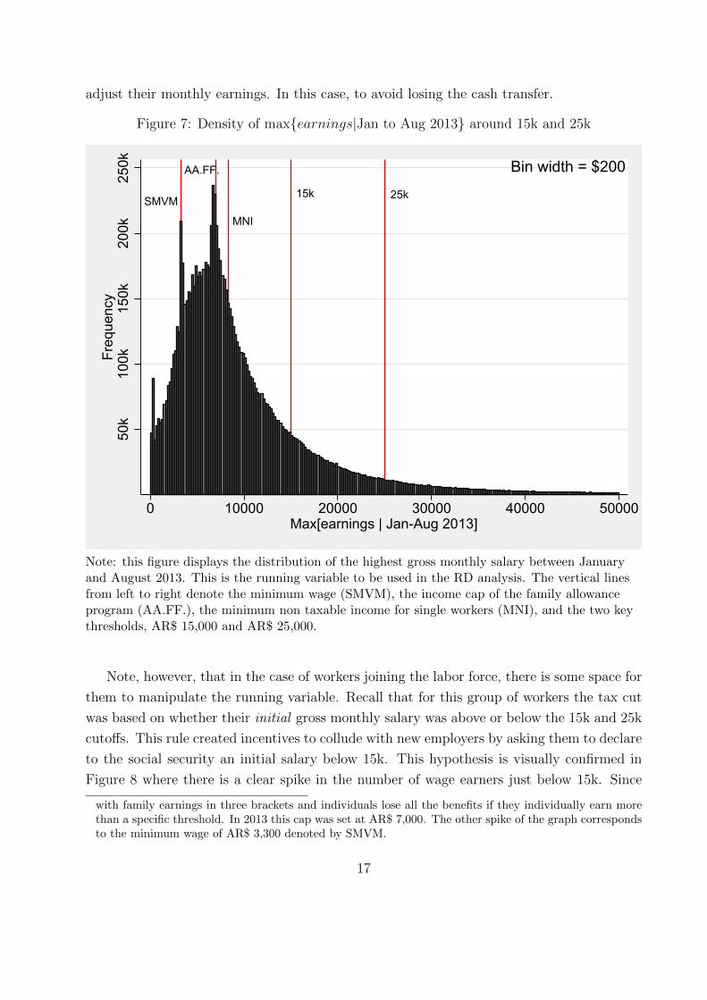
adjust their monthly earnings. In this case, to avoid losing the cash transfer.
Figure 7: Density of max{earnings|Jan to Aug 2013} around 15k and 25k50
k10
0k15
0k20
0k25
0kFr
eque
ncy
0 10000 20000 30000 40000 50000Max[earnings | Jan-Aug 2013]
Bin width = $200
25k15kSMVM
MNI
AA.FF.
Note: this figure displays the distribution of the highest gross monthly salary between Januaryand August 2013. This is the running variable to be used in the RD analysis. The vertical linesfrom left to right denote the minimum wage (SMVM), the income cap of the family allowanceprogram (AA.FF.), the minimum non taxable income for single workers (MNI), and the two keythresholds, AR$ 15,000 and AR$ 25,000.
Note, however, that in the case of workers joining the labor force, there is some space for
them to manipulate the running variable. Recall that for this group of workers the tax cut
was based on whether their initial gross monthly salary was above or below the 15k and 25k
cutoffs. This rule created incentives to collude with new employers by asking them to declare
to the social security an initial salary below 15k. This hypothesis is visually confirmed in
Figure 8 where there is a clear spike in the number of wage earners just below 15k. Since
with family earnings in three brackets and individuals lose all the benefits if they individually earn morethan a specific threshold. In 2013 this cap was set at AR$ 7,000. The other spike of the graph correspondsto the minimum wage of AR$ 3,300 denoted by SMVM.
17
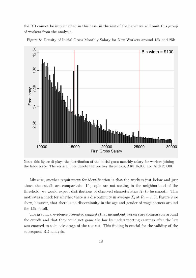
the RD cannot be implemented in this case, in the rest of the paper we will omit this group
of workers from the analysis.
Figure 8: Density of Initial Gross Monthly Salary for New Workers around 15k and 25k
2.5k
5k7.
5k10
k12
.5k
Freq
uenc
y
10000 15000 20000 25000 30000First Gross Salary
Bin width = $100
Note: this figure displays the distribution of the initial gross monthly salary for workers joiningthe labor force. The vertical lines denote the two key thresholds, AR$ 15,000 and AR$ 25,000.
Likewise, another requirement for identification is that the workers just below and just
above the cutoffs are comparable. If people are not sorting in the neighborhood of the
threshold, we would expect distributions of observed characteristics Xi to be smooth. This
motivates a check for whether there is a discontinuity in average Xi at Ri = c. In Figure 9 we
show, however, that there is no discontinuity in the age and gender of wage earners around
the 15k cutoff.
The graphical evidence presented suggests that incumbent workers are comparable around
the cutoffs and that they could not game the law by underreporting earnings after the law
was enacted to take advantage of the tax cut. This finding is crucial for the validity of the
subsequent RD analysis.
18
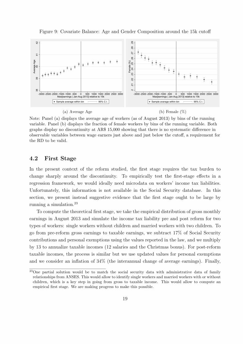
Figure 9: Covariate Balance: Age and Gender Composition around the 15k cutoff38
3940
4142
Aver
age
Age
-3000 -2500 -2000 -1500 -1000 -500 0 500 1000 1500 2000 2500 3000Max[earnings | Jan-Aug 2013] relative to 15k
Sample average within bin 95% C.I.
(a) Average Age
.2.2
1.2
2.2
3.2
4.2
5.2
6.2
7.2
8.2
9Fe
mal
e (%
)
-3000 -2500 -2000 -1500 -1000 -500 0 500 1000 1500 2000 2500 3000Max[earnings | Jan-Aug 2013] relative to 15k
Sample average within bin 95% C.I.
(b) Female (%)
Note: Panel (a) displays the average age of workers (as of August 2013) by bins of the runningvariable. Panel (b) displays the fraction of female workers by bins of the running variable. Bothgraphs display no discontinuity at AR$ 15,000 showing that there is no systematic difference inobservable variables between wage earners just above and just below the cutoff, a requirement forthe RD to be valid.
4.2 First Stage
In the present context of the reform studied, the first stage requires the tax burden to
change sharply around the discontinuity. To empirically test the first-stage effects in a
regression framework, we would ideally need microdata on workers’ income tax liabilities.
Unfortunately, this information is not available in the Social Security database. In this
section, we present instead suggestive evidence that the first stage ought to be large by
running a simulation.23
To compute the theoretical first stage, we take the empirical distribution of gross monthly
earnings in August 2013 and simulate the income tax liability pre and post reform for two
types of workers: single workers without children and married workers with two children. To
go from pre-reform gross earnings to taxable earnings, we subtract 17% of Social Security
contributions and personal exemptions using the values reported in the law, and we multiply
by 13 to annualize taxable incomes (12 salaries and the Christmas bonus). For post-reform
taxable incomes, the process is similar but we use updated values for personal exemptions
and we consider an inflation of 34% (the interannual change of average earnings). Finally,
23One partial solution would be to match the social security data with administrative data of familyrelationships from ANSES. This would allow to identify single workers and married workers with or withoutchildren, which is a key step in going from gross to taxable income. This would allow to compute anempirical first stage. We are making progress to make this possible.
19
we take pre- and post-reform annual taxable incomes to Table 1 in order to compute the
income tax and corresponding marginal tax rate.
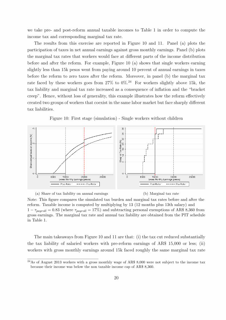
The results from this exercise are reported in Figure 10 and 11. Panel (a) plots the
participation of taxes in net annual earnings against gross monthly earnings. Panel (b) plots
the marginal tax rates that workers would face at different parts of the income distribution
before and after the reform. For example, Figure 10 (a) shows that single workers earning
slightly less than 15k pesos went from paying around 10 percent of annual earnings in taxes
before the reform to zero taxes after the reform. Moreover, in panel (b) the marginal tax
rate faced by these workers goes from 27% to 0%.24 For workers slightly above 15k, the
tax liability and marginal tax rate increased as a consequence of inflation and the “bracket
creep”. Hence, without loss of generality, this example illustrates how the reform effectively
created two groups of workers that coexist in the same labor market but face sharply different
tax liabilities.
Figure 10: First stage (simulation) - Single workers without children
(a) Share of tax liability on annual earnings (b) Marginal tax rate
Note: This figure compares the simulated tax burden and marginal tax rates before and after thereform. Taxable income is computed by multiplying by 13 (12 months plus 13th salary) and1− τpayroll = 0.83 (where τpayroll = 17%) and subtracting personal exemptions of AR$ 8,360 fromgross earnings. The marginal tax rate and annual tax liability are obtained from the PIT schedulein Table 1.
The main takeaways from Figure 10 and 11 are that: (i) the tax cut reduced substantially
the tax liability of salaried workers with pre-reform earnings of AR$ 15,000 or less; (ii)
workers with gross monthly earnings around 15k faced roughly the same marginal tax rate
24As of August 2013 workers with a gross monthly wage of AR$ 8,000 were not subject to the income taxbecause their income was below the non taxable income cap of AR$ 8,360.
20
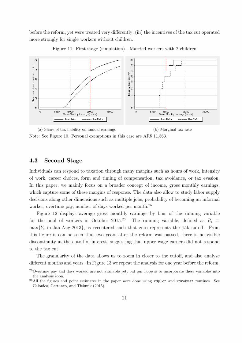
before the reform, yet were treated very differently; (iii) the incentives of the tax cut operated
more strongly for single workers without children.
Figure 11: First stage (simulation) - Married workers with 2 children
(a) Share of tax liability on annual earnings (b) Marginal tax rate
Note: See Figure 10. Personal exemptions in this case are AR$ 11,563.
4.3 Second Stage
Individuals can respond to taxation through many margins such as hours of work, intensity
of work, career choices, form and timing of compensation, tax avoidance, or tax evasion.
In this paper, we mainly focus on a broader concept of income, gross monthly earnings,
which capture some of these margins of response. The data also allow to study labor supply
decisions along other dimensions such as multiple jobs, probability of becoming an informal
worker, overtime pay, number of days worked per month.25
Figure 12 displays average gross monthly earnings by bins of the running variable
for the pool of workers in October 2015.26 The running variable, defined as Ri ≡max{Yi in Jan-Aug 2013}, is recentered such that zero represents the 15k cutoff. From
this figure it can be seen that two years after the reform was passed, there is no visible
discontinuity at the cutoff of interest, suggesting that upper wage earners did not respond
to the tax cut.
The granularity of the data allows us to zoom in closer to the cutoff, and also analyze
different months and years. In Figure 13 we repeat the analysis for one year before the reform,
25Overtime pay and days worked are not available yet, but our hope is to incorporate these variables intothe analysis soon.
26All the figures and point estimates in the paper were done using rdplot and rdrobust routines. SeeCalonico, Cattaneo, and Titiunik (2015).
21
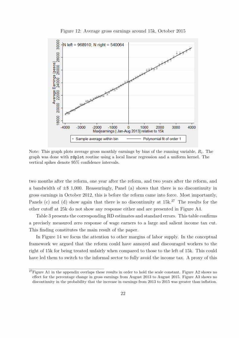
Figure 12: Average gross earnings around 15k, October 2015
Note: This graph plots average gross monthly earnings by bins of the running variable, Ri. Thegraph was done with rdplot routine using a local linear regression and a uniform kernel. Thevertical spikes denote 95% confidence intervals.
two months after the reform, one year after the reform, and two years after the reform, and
a bandwidth of ±$ 1,000. Reassuringly, Panel (a) shows that there is no discontinuity in
gross earnings in October 2012, this is before the reform came into force. Most importantly,
Panels (c) and (d) show again that there is no discontinuity at 15k.27 The results for the
other cutoff at 25k do not show any response either and are presented in Figure A4.
Table 3 presents the corresponding RD estimates and standard errors. This table confirms
a precisely measured zero response of wage earners to a large and salient income tax cut.
This finding constitutes the main result of the paper.
In Figure 14 we focus the attention to other margins of labor supply. In the conceptual
framework we argued that the reform could have annoyed and discouraged workers to the
right of 15k for being treated unfairly when compared to those to the left of 15k. This could
have led them to switch to the informal sector to fully avoid the income tax. A proxy of this
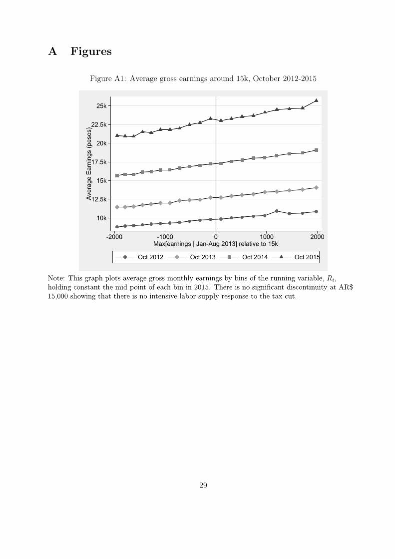
27Figure A1 in the appendix overlaps these results in order to hold the scale constant. Figure A2 shows noeffect for the percentage change in gross earnings from August 2013 to August 2015. Figure A3 shows nodiscontinuity in the probability that the increase in earnings from 2013 to 2015 was greater than inflation.
22
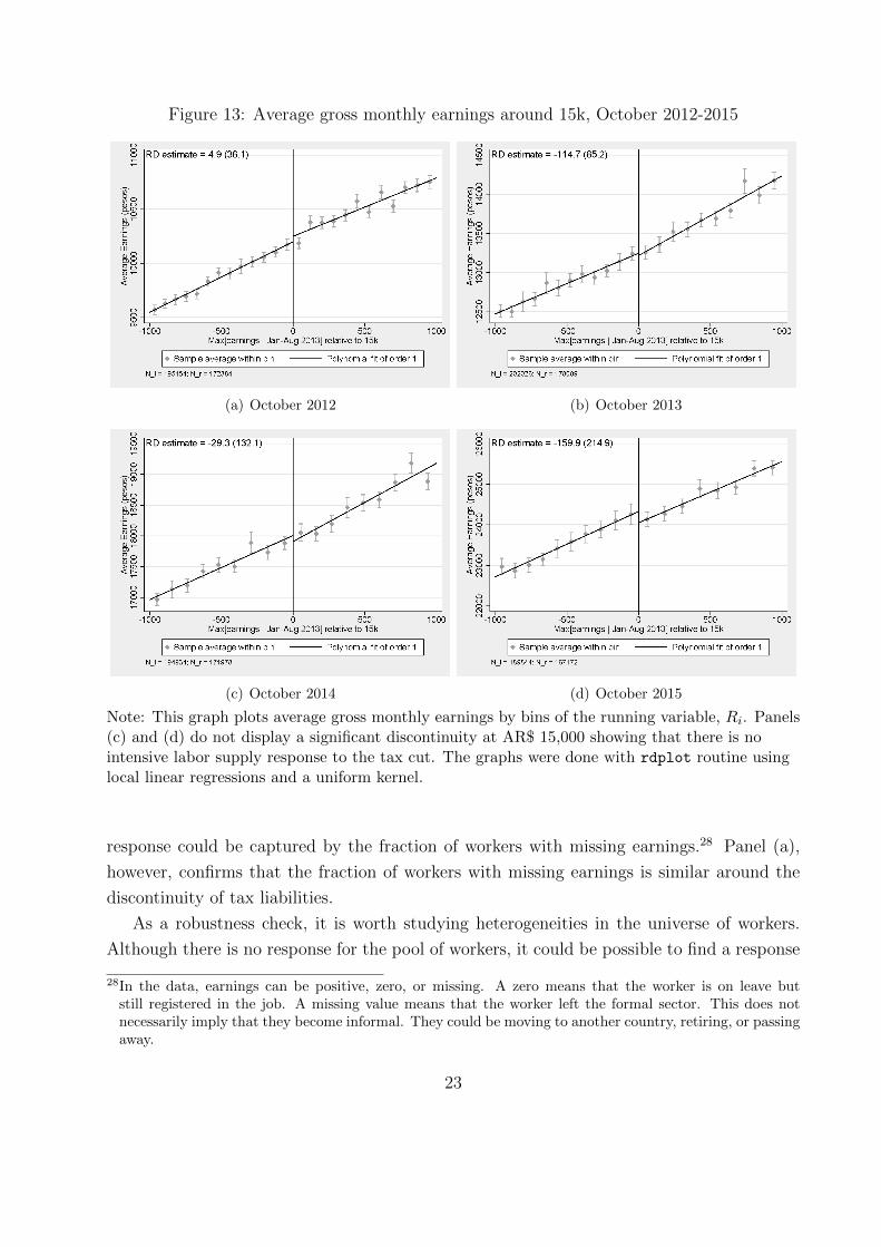
Figure 13: Average gross monthly earnings around 15k, October 2012-2015
(a) October 2012 (b) October 2013
(c) October 2014 (d) October 2015
Note: This graph plots average gross monthly earnings by bins of the running variable, Ri. Panels(c) and (d) do not display a significant discontinuity at AR$ 15,000 showing that there is nointensive labor supply response to the tax cut. The graphs were done with rdplot routine usinglocal linear regressions and a uniform kernel.
response could be captured by the fraction of workers with missing earnings.28 Panel (a),
however, confirms that the fraction of workers with missing earnings is similar around the
discontinuity of tax liabilities.
As a robustness check, it is worth studying heterogeneities in the universe of workers.
Although there is no response for the pool of workers, it could be possible to find a response
28In the data, earnings can be positive, zero, or missing. A zero means that the worker is on leave butstill registered in the job. A missing value means that the worker left the formal sector. This does notnecessarily imply that they become informal. They could be moving to another country, retiring, or passingaway.
23
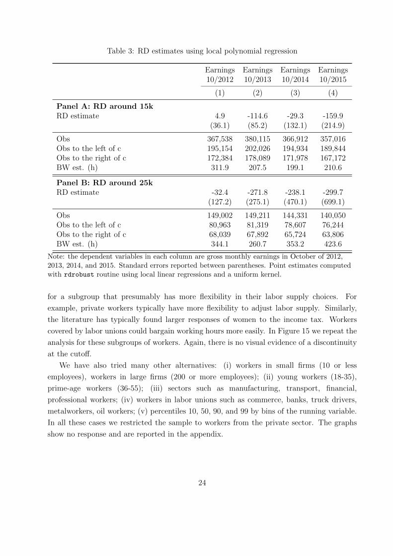
Table 3: RD estimates using local polynomial regression
Earnings Earnings Earnings Earnings10/2012 10/2013 10/2014 10/2015
(1) (2) (3) (4)
Panel A: RD around 15kRD estimate 4.9 -114.6 -29.3 -159.9
(36.1) (85.2) (132.1) (214.9)
Obs 367,538 380,115 366,912 357,016Obs to the left of c 195,154 202,026 194,934 189,844Obs to the right of c 172,384 178,089 171,978 167,172BW est. (h) 311.9 207.5 199.1 210.6
Panel B: RD around 25kRD estimate -32.4 -271.8 -238.1 -299.7
(127.2) (275.1) (470.1) (699.1)
Obs 149,002 149,211 144,331 140,050Obs to the left of c 80,963 81,319 78,607 76,244Obs to the right of c 68,039 67,892 65,724 63,806BW est. (h) 344.1 260.7 353.2 423.6
Note: the dependent variables in each column are gross monthly earnings in October of 2012,2013, 2014, and 2015. Standard errors reported between parentheses. Point estimates computedwith rdrobust routine using local linear regressions and a uniform kernel.
for a subgroup that presumably has more flexibility in their labor supply choices. For
example, private workers typically have more flexibility to adjust labor supply. Similarly,
the literature has typically found larger responses of women to the income tax. Workers
covered by labor unions could bargain working hours more easily. In Figure 15 we repeat the
analysis for these subgroups of workers. Again, there is no visual evidence of a discontinuity
at the cutoff.
We have also tried many other alternatives: (i) workers in small firms (10 or less
employees), workers in large firms (200 or more employees); (ii) young workers (18-35),
prime-age workers (36-55); (iii) sectors such as manufacturing, transport, financial,
professional workers; (iv) workers in labor unions such as commerce, banks, truck drivers,
metalworkers, oil workers; (v) percentiles 10, 50, 90, and 99 by bins of the running variable.
In all these cases we restricted the sample to workers from the private sector. The graphs
show no response and are reported in the appendix.
24
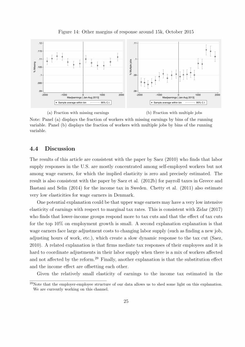
Figure 14: Other margins of response around 15k, October 2015
.09
.095
.1
.105
.11
.115
.12
% M
issi
ng
-2000 -1000 0 1000 2000Max[earnings | Jan-Aug 2013]
Sample average within bin 95% C.I.
(a) Fraction with missing earnings
.08
.09
.1
.11
% M
ultip
le jo
bs
-2000 -1000 0 1000 2000Max[earnings | Jan-Aug 2013]
Sample average within bin 95% C.I.
(b) Fraction with multiple jobs
Note: Panel (a) displays the fraction of workers with missing earnings by bins of the runningvariable. Panel (b) displays the fraction of workers with multiple jobs by bins of the runningvariable.
4.4 Discussion
The results of this article are consistent with the paper by Saez (2010) who finds that labor
supply responses in the U.S. are mostly concentrated among self-employed workers but not
among wage earners, for which the implied elasticity is zero and precisely estimated. The
result is also consistent with the paper by Saez et al. (2012b) for payroll taxes in Greece and
Bastani and Selin (2014) for the income tax in Sweden. Chetty et al. (2011) also estimate
very low elasticities for wage earners in Denmark.
One potential explanation could be that upper wage earners may have a very low intensive
elasticity of earnings with respect to marginal tax rates. This is consistent with Zidar (2017)
who finds that lower-income groups respond more to tax cuts and that the effect of tax cuts
for the top 10% on employment growth is small. A second explanation explanation is that
wage earners face large adjustment costs to changing labor supply (such as finding a new job,
adjusting hours of work, etc.), which create a slow dynamic response to the tax cut (Saez,
2010). A related explanation is that firms mediate tax responses of their employees and it is
hard to coordinate adjustments in their labor supply when there is a mix of workers affected
and not affected by the reform.29 Finally, another explanation is that the substitution effect
and the income effect are offsetting each other.
Given the relatively small elasticity of earnings to the income tax estimated in the
29Note that the employer-employee structure of our data allows us to shed some light on this explanation.We are currently working on this channel.
25
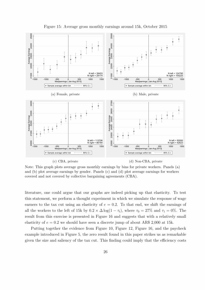
Figure 15: Average gross monthly earnings around 15k, October 201521
000
2200
023
000
2400
025
000
Aver
age
Earn
ings
-1500 -1000 -500 0 500 1000 1500Max[earnings | Jan-Aug 2013]
Sample average within bin 95% C.I.
N left = 39453N right = 29174
(a) Female, private
2100
022
000
2300
024
000
2500
0Av
erag
e Ea
rnin
gs
-1500 -1000 -500 0 500 1000 1500Max[earnings | Jan-Aug 2013]
Sample average within bin 95% C.I.
N left = 124795N right = 100225
(b) Male, private
2000
021
000
2200
023
000
2400
0Av
erag
e Ea
rnin
gs
-1500 -1000 -500 0 500 1000 1500Max[earnings | Jan-Aug 2013]
Sample average within bin 95% C.I.
N left = 113706N right = 86784
(c) CBA, private
2200
023
000
2400
025
000
2600
027
000
Aver
age
Earn
ings
-1500 -1000 -500 0 500 1000 1500Max[earnings | Jan-Aug 2013]
Sample average within bin 95% C.I.
N left = 50550N right = 42623
(d) Non-CBA, private
Note: This graph plots average gross monthly earnings by bins for private workers. Panels (a)and (b) plot average earnings by gender. Panels (c) and (d) plot average earnings for workerscovered and not covered by collective bargaining agreements (CBA).
literature, one could argue that our graphs are indeed picking up that elasticity. To test
this statement, we perform a thought experiment in which we simulate the response of wage
earners to the tax cut using an elasticity of e = 0.2. To that end, we shift the earnings of
all the workers to the left of 15k by 0.2×∆ log(1− τt), where τ0 = 27% and τ1 = 0%. The
result from this exercise is presented in Figure 16 and suggests that with a relatively small
elasticity of e = 0.2 we should have seen a discrete jump of about AR$ 2,000 at 15k.
Putting together the evidence from Figure 10, Figure 12, Figure 16, and the paycheck
example introduced in Figure 5, the zero result found in this paper strikes us as remarkable
given the size and saliency of the tax cut. This finding could imply that the efficiency costs
26
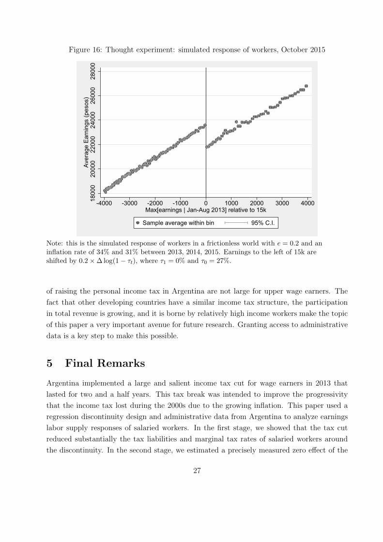
Figure 16: Thought experiment: simulated response of workers, October 2015
1800
020
000
2200
024
000
2600
028
000
Aver
age
Earn
ings
(pes
os)
-4000 -3000 -2000 -1000 0 1000 2000 3000 4000Max[earnings | Jan-Aug 2013] relative to 15k
Sample average within bin 95% C.I.
Note: this is the simulated response of workers in a frictionless world with e = 0.2 and aninflation rate of 34% and 31% between 2013, 2014, 2015. Earnings to the left of 15k areshifted by 0.2×∆ log(1− τt), where τ1 = 0% and τ0 = 27%.
of raising the personal income tax in Argentina are not large for upper wage earners. The
fact that other developing countries have a similar income tax structure, the participation
in total revenue is growing, and it is borne by relatively high income workers make the topic
of this paper a very important avenue for future research. Granting access to administrative
data is a key step to make this possible.
5 Final Remarks
Argentina implemented a large and salient income tax cut for wage earners in 2013 that
lasted for two and a half years. This tax break was intended to improve the progressivity
that the income tax lost during the 2000s due to the growing inflation. This paper used a
regression discontinuity design and administrative data from Argentina to analyze earnings
labor supply responses of salaried workers. In the first stage, we showed that the tax cut
reduced substantially the tax liabilities and marginal tax rates of salaried workers around
the discontinuity. In the second stage, we estimated a precisely measured zero effect of the
27
tax cut on labor earnings around the discontinuity two years after the reform. This finding
suggests that upper wage earners (about decile 8) were not responsive to a large and salient
tax cut. Anecdotal evidence from newspapers and paychecks confirm saliency and relevance
of the reform. Our findings could imply that the costs of raising income taxes in developing
countries are not large, at least for the intensive margin and upper income earners. External
validity remains an open question.
References
Bastani, S., Selin, H., (2014). Bunching and non-bunching at kink points of the Swedish taxschedule. Journal of Public Economics, 109 (C), 36–49.
Calonico, S., M. D. Cattaneo, and R. Titiunik. (2015). Optimal Data-Driven RegressionDiscontinuity Plots. Journal of the American Statistical Association 110(512): 1753-1769.
Cavallo, A., and M. Bertolotto. (2016). Filling the Gap in Argentina’s Inflation Data.mimeo.
Chetty, R., Friedman, J., Olsen, T., Pistaferri, L., (2011). Adjustment costs, firm responses,and micro vs. macro labor supply elasticities: evidence from Danish tax records. QuarterlyJournal of Economics, 126, 749–804.
Saez, E. (2003). The Effect of Marginal Tax Rates on Income: A Panel Study of ‘BracketCreep’. Journal of Public Economics, 87: 1231-1258.
Saez, E. (2010). Do Taxpayers Bunch at Kink Points?, American Economic Journal:Economic Policy, American Economic Association, vol. 2(3), pages 180-212, August.
Saez, E., Slemrod, J., and Giertz, S. H. (2012a). The Elasticity of Taxable Income withRespect to Marginal Tax Rates: A Critical Review. Journal of Economic Literature, 50(1):3–50.
Saez, E., Matsaganis, M., and Tsakloglou, P. (2012b). Earnings Determination andTaxes: Evidence From a Cohort-Based Payroll Tax Reform in Greece, Quarterly Journalof Economics, 127 (1), 493-533.
Weber, C. E. (2014). Toward Obtaining a Consistent Estimate of the Elasticity of TaxableIncome using Difference-in-Differences. Journal of Public Economics, 117:90–103.
Yagan, D. (2015). Capital tax reform and the real economy: The effects of the 2003 dividendtax cut. The American Economic Review, 105(12), 3531-3563.
Zidar, O. M. (2017). Tax Cuts For Whom? Heterogeneous Effects of Income Tax Changeson Growth and Employment,NBER Working Paper No. 21035.
28
A Figures
Figure A1: Average gross earnings around 15k, October 2012-2015
10k
12.5k
15k
17.5k
20k
22.5k
25k
Aver
age
Earn
ings
(pes
os)
-2000 -1000 0 1000 2000Max[earnings | Jan-Aug 2013] relative to 15k
Oct 2012 Oct 2013 Oct 2014 Oct 2015
Note: This graph plots average gross monthly earnings by bins of the running variable, Ri,holding constant the mid point of each bin in 2015. There is no significant discontinuity at AR$15,000 showing that there is no intensive labor supply response to the tax cut.
29
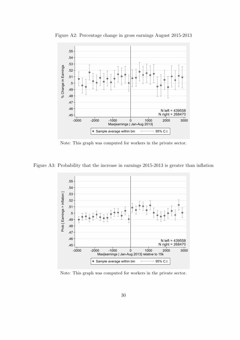
Figure A2: Percentage change in gross earnings August 2015-2013
.45
.46
.47
.48
.49
.5
.51
.52
.53
.54
.55
% C
hang
e in
Ear
ning
s
-3000 -2000 -1000 0 1000 2000 3000Max[earnings | Jan-Aug 2013]
Sample average within bin 95% C.I.
N left = 439558N right = 268470
Note: This graph was computed for workers in the private sector.
Figure A3: Probability that the increase in earnings 2015-2013 is greater than inflation
.45
.46
.47
.48
.49
.5
.51
.52
.53
.54
.55
Prob
[ Ea
rnin
gs >
infla
tion
]
-3000 -2000 -1000 0 1000 2000 3000Max[earnings | Jan-Aug 2013] relative to 15k
Sample average within bin 95% C.I.
N left = 439558N right = 268470
Note: This graph was computed for workers in the private sector.
30
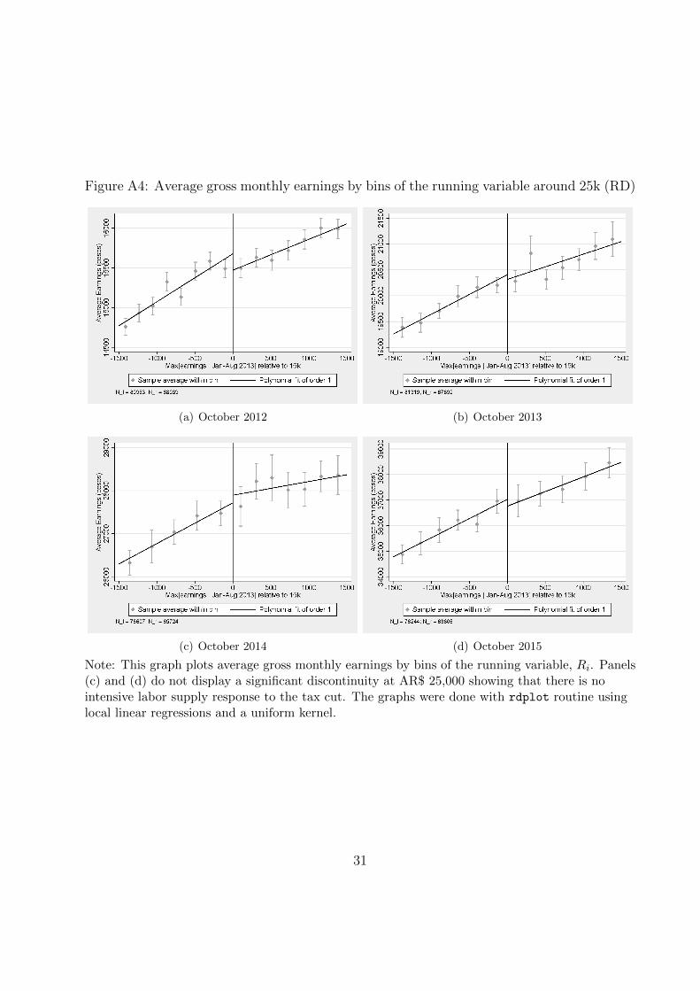
Figure A4: Average gross monthly earnings by bins of the running variable around 25k (RD)
(a) October 2012 (b) October 2013
(c) October 2014 (d) October 2015
Note: This graph plots average gross monthly earnings by bins of the running variable, Ri. Panels(c) and (d) do not display a significant discontinuity at AR$ 25,000 showing that there is nointensive labor supply response to the tax cut. The graphs were done with rdplot routine usinglocal linear regressions and a uniform kernel.
31
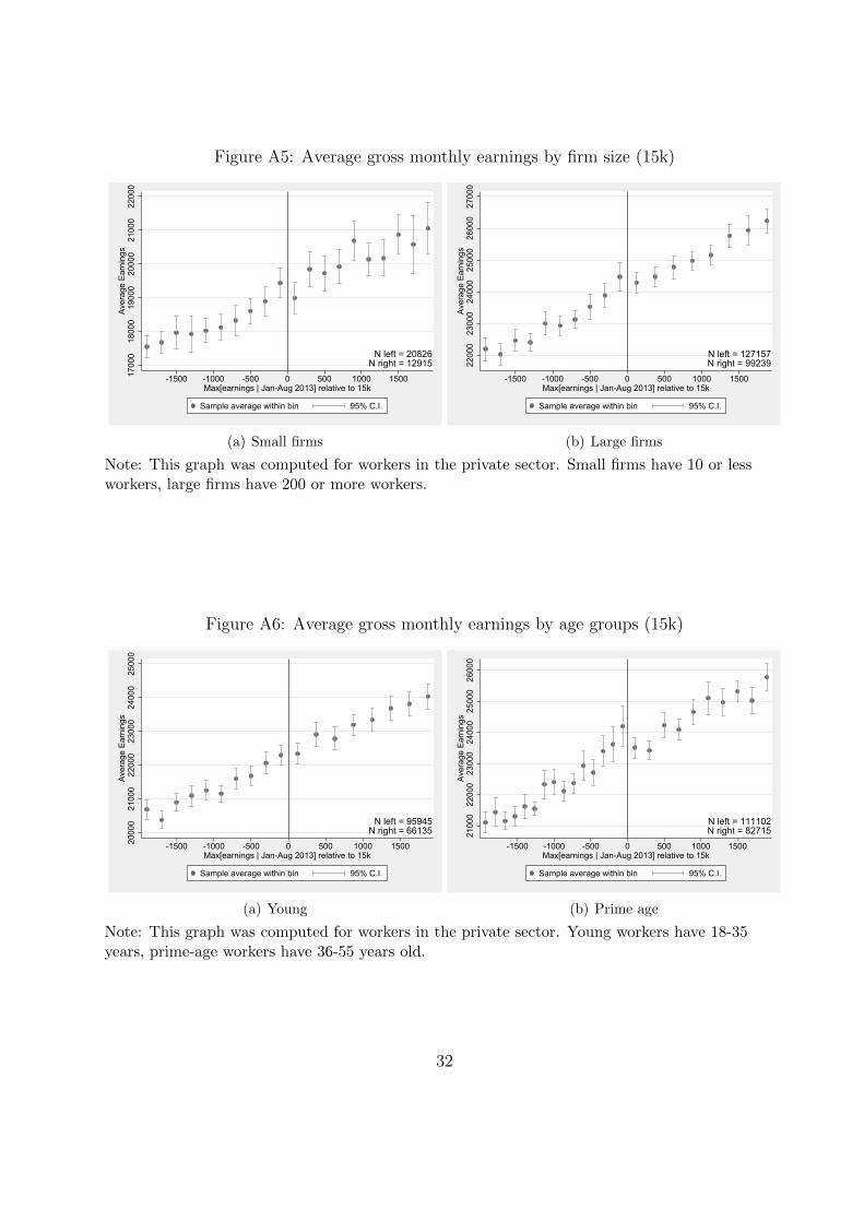
Figure A5: Average gross monthly earnings by firm size (15k)
1700
018
000
1900
020
000
2100
022
000
Aver
age
Earn
ings
-1500 -1000 -500 0 500 1000 1500Max[earnings | Jan-Aug 2013] relative to 15k
Sample average within bin 95% C.I.
N left = 20826N right = 12915
(a) Small firms
2200
023
000
2400
025
000
2600
027
000
Aver
age
Earn
ings
-1500 -1000 -500 0 500 1000 1500Max[earnings | Jan-Aug 2013] relative to 15k
Sample average within bin 95% C.I.
N left = 127157N right = 99239
(b) Large firms
Note: This graph was computed for workers in the private sector. Small firms have 10 or lessworkers, large firms have 200 or more workers.
Figure A6: Average gross monthly earnings by age groups (15k)
2000
021
000
2200
023
000
2400
025
000
Aver
age
Earn
ings
-1500 -1000 -500 0 500 1000 1500Max[earnings | Jan-Aug 2013] relative to 15k
Sample average within bin 95% C.I.
N left = 95945N right = 66135
(a) Young
2100
022
000
2300
024
000
2500
026
000
Aver
age
Earn
ings
-1500 -1000 -500 0 500 1000 1500Max[earnings | Jan-Aug 2013] relative to 15k
Sample average within bin 95% C.I.
N left = 111102N right = 82715
(b) Prime age
Note: This graph was computed for workers in the private sector. Young workers have 18-35years, prime-age workers have 36-55 years old.
32
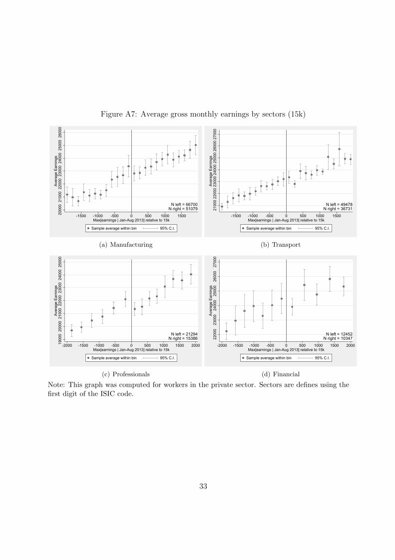
Figure A7: Average gross monthly earnings by sectors (15k)
2000
021
000
2200
023
000
2400
025
000
2600
0Av
erag
e Ea
rnin
gs
-1500 -1000 -500 0 500 1000 1500Max[earnings | Jan-Aug 2013] relative to 15k
Sample average within bin 95% C.I.
N left = 66700N right = 51079
(a) Manufacturing
2100
022
000
2300
024
000
2500
026
000
2700
0Av
erag
e Ea
rnin
gs-1500 -1000 -500 0 500 1000 1500
Max[earnings | Jan-Aug 2013] relative to 15k
Sample average within bin 95% C.I.
N left = 49478N right = 36731
(b) Transport
1900
020
000
2100
022
000
2300
024
000
2500
0Av
erag
e Ea
rnin
gs
-2000 -1500 -1000 -500 0 500 1000 1500 2000Max[earnings | Jan-Aug 2013] relative to 15k
Sample average within bin 95% C.I.
N left = 21294N right = 15386
(c) Professionals
2200
023
000
2400
025
000
2600
027
000
Aver
age
Earn
ings
-2000 -1500 -1000 -500 0 500 1000 1500 2000Max[earnings | Jan-Aug 2013] relative to 15k
Sample average within bin 95% C.I.
N left = 12452N right = 10347
(d) Financial
Note: This graph was computed for workers in the private sector. Sectors are defines using thefirst digit of the ISIC code.
33
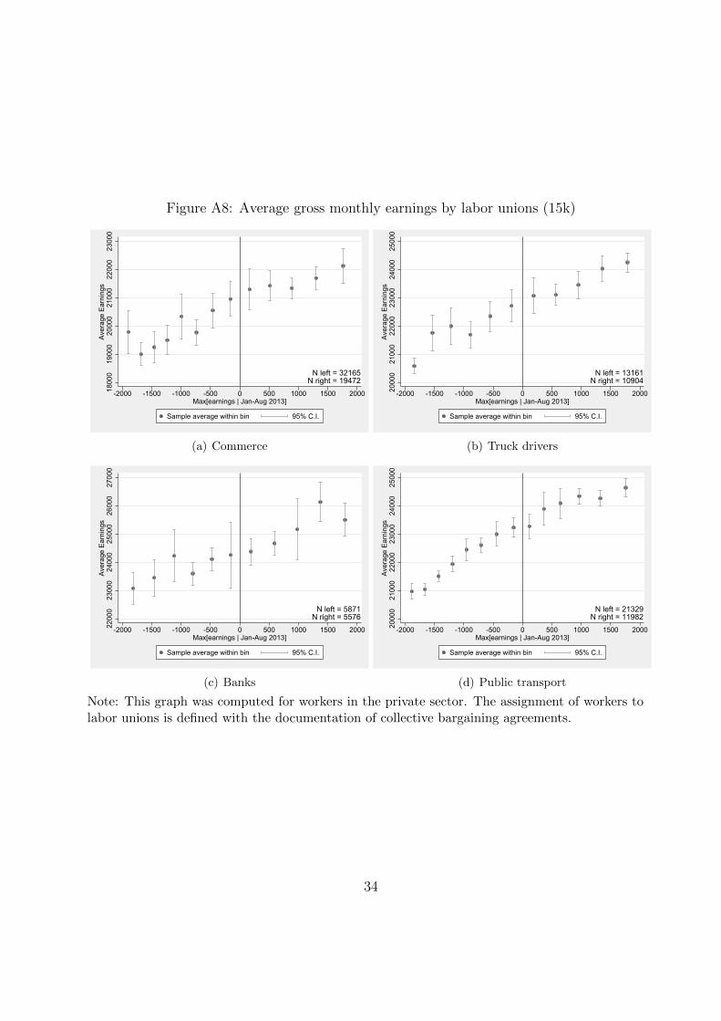
Figure A8: Average gross monthly earnings by labor unions (15k)
1800
019
000
2000
021
000
2200
023
000
Aver
age
Earn
ings
-2000 -1500 -1000 -500 0 500 1000 1500 2000Max[earnings | Jan-Aug 2013]
Sample average within bin 95% C.I.
N left = 32165N right = 19472
(a) Commerce
2000
021
000
2200
023
000
2400
025
000
Aver
age
Earn
ings
-2000 -1500 -1000 -500 0 500 1000 1500 2000Max[earnings | Jan-Aug 2013]
Sample average within bin 95% C.I.
N left = 13161N right = 10904
(b) Truck drivers
2200
023
000
2400
025
000
2600
027
000
Aver
age
Earn
ings
-2000 -1500 -1000 -500 0 500 1000 1500 2000Max[earnings | Jan-Aug 2013]
Sample average within bin 95% C.I.
N left = 5871N right = 5576
(c) Banks
2000
021
000
2200
023
000
2400
025
000
Aver
age
Earn
ings
-2000 -1500 -1000 -500 0 500 1000 1500 2000Max[earnings | Jan-Aug 2013]
Sample average within bin 95% C.I.
N left = 21329N right = 11982
(d) Public transport
Note: This graph was computed for workers in the private sector. The assignment of workers tolabor unions is defined with the documentation of collective bargaining agreements.
34
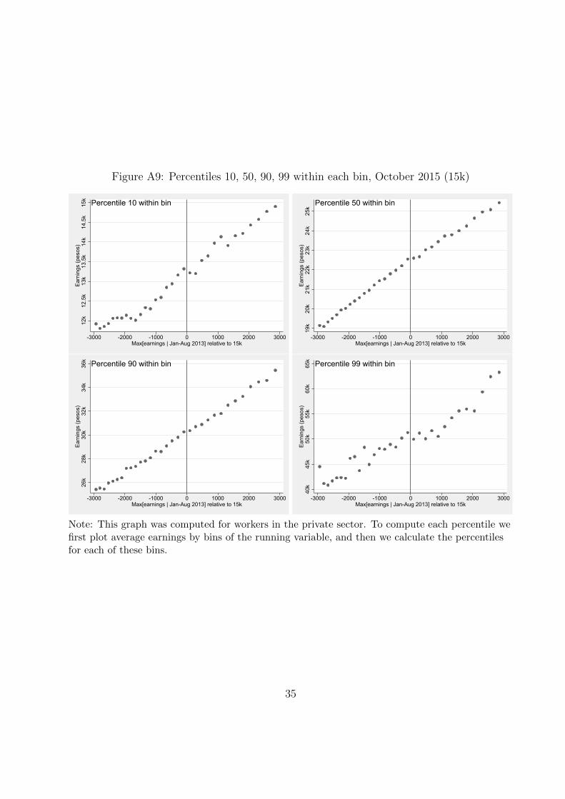
Figure A9: Percentiles 10, 50, 90, 99 within each bin, October 2015 (15k)
12k
12.5
k13
k13
.5k
14k
14.5
k15
kEa
rnin
gs (p
esos
)
-3000 -2000 -1000 0 1000 2000 3000Max[earnings | Jan-Aug 2013] relative to 15k
Percentile 10 within bin
19k
20k
21k
22k
23k
24k
25k
Earn
ings
(pes
os)
-3000 -2000 -1000 0 1000 2000 3000Max[earnings | Jan-Aug 2013] relative to 15k
Percentile 50 within bin
26k
28k
30k
32k
34k
36k
Earn
ings
(pes
os)
-3000 -2000 -1000 0 1000 2000 3000Max[earnings | Jan-Aug 2013] relative to 15k
Percentile 90 within bin
40k
45k
50k
55k
60k
65k
Earn
ings
(pes
os)
-3000 -2000 -1000 0 1000 2000 3000Max[earnings | Jan-Aug 2013] relative to 15k
Percentile 99 within bin
Note: This graph was computed for workers in the private sector. To compute each percentile wefirst plot average earnings by bins of the running variable, and then we calculate the percentilesfor each of these bins.
35