Pollcy, Research, and External Affairs

WORKING PAPERS

Debt and International Finance

International Economics DepartmentThe World Bank

July 1991WPS 721

The Demand for Moneyin Developing Countries

Assessing the Roleof Financial Innovation

Patricio ArrauJosb De GregorioCarmen Reinhart

andPeter Wickham

Financial innovation is important in determining the demand formoney and its fluctuations, importance that increases with therate of inflation.

ThePolicy,Research, and Extemal Affairs Complex d.stnbutes PRE Working Papers todisserunatethe ftndungsof work in progress andto eneourage the exchange of ideas among Bank staff and all others interested in development issues. These papers carry the names ofthe authors, rflect only their views, and should be used and cited accordingly. The findings, interpretations, and conclusions are theauthors' own. Itey should not be attributed to the World Bank, its Board of Directors, its managanent, or any of its memner countries.

Pub

lic D

iscl

osur

e A

utho

rized

Pub

lic D

iscl

osur

e A

utho

rized

Pub

lic D

iscl

osur

e A

utho

rized

Pub

lic D

iscl

osur

e A

utho

rized

Pub

lic D

iscl

osur

e A

utho

rized

Pub

lic D

iscl

osur

e A

utho

rized

Pub

lic D

iscl

osur

e A

utho

rized

Pub

lic D

iscl

osur

e A

utho

rized

Poiy, Research, and External Affairs

Debt and International Finance

WPS 721

This paper - a joint product of the Debt and International Finance Division, International EconomicsDepartnent and the International Monetary Fund - is part of a largereffort in PRE to apply new monetaryapproaches to developing countries. It is also being distributed as an IMF working paper. Copies areavailable free from the World Bank, 1818 H Street NW, Washington DC 20433. Please contact SheilahKing-Watson, room S8-040, extension 31047 (44 pages, with figures and tables).

Traditional specifications of money demand financial innovation. They also assess thehave commonly been plagued by persistent relative importance of this variable.overprediction, implausible parameter estimates,and highly autocorrelated errors. They find that financial innovation can be

better modeled as a stochastic (random-walk)Arrau, Dc Gregorio, Reinhart, and Wickham trend rather than a deterministic (time) trend.

argue that some of these problems stem from the Financial innovation plays an important role infailure to account for the impact of financial determining fluctuations of the demand forinnovation. money. The importance of this role increases

with the rate of inflation.They estimate money demand for ten

developing countries, using various proxies for

The PRE Working Paper Scries disseminates the findings of work under way in the Bank's Policy. Research, and ExtemalAffairsComplex. Anobjectiveoftheseries is toget thesefindingsoutquickly, even if presentations are less than fullypolished.T'he findings, interpretations, and conclusions in these papers do not necessarily represent official Bank policy.

Produced by the PRE Dissemination Center

The Demand for Money in Developing Countries:Assessing the Role of Financial Innovation

byPatricio Arrau, Jose De Gregorio,

Carmen Reinhart, and Peter Wickham*

Table of Contents

I. Introduction 1

II. Theoretical Framework 3

1. Households' demand for money 42. Firms' demand for money: A transactions cost model 63. Aggregation issues 84. The opportunity cost of money 9

III. Failure of Traditional Approaches 11

1. Data and specification issues 132. Empirical results 14

IV. The Extended Model: Alternative Approaches to Modeling Financial 16Innovation

1. Is a deterministric trend a good proxy for financial innovation? 172. Is a stochastic trend a good proxy for financial innovation? 193. Is the role of financial innovation large or small? 23

V. Concluding Remarks 27

Appendix A: Discussion on Aggregation and the Regression Error 31

Appendix B: Estimation with a Time-Varying Intercept 34

References 36

* The authors would like to thank Bela Balassa and Greg Hess for valuablecomments to a previous version. This paper is also being distributed as an IMF workingpaper.

I. INTRODUCTION

From standard IS-LM models and their extension to open economies in the

Mundell-Fleming manner to international monetary models and "new" classical

models, money plays a central role. The demand for money serves as a

conduit in the transmission mechanism for both monetary and fiscal policy in

these types of models, so that the stability of the money demand function is

critical if monetary and fiscal policy are to have predictable effects over

time on real output and the price level. As well as being at the heart of

the issue of monetary policy effectiveness, the demand for money is

important in assessing the welfare implications of policy changes and for

determining the role of seignorage in an economy.

In criticisms of the various analytical approaches commonly used in

policy assessments, it is frequently questioned whether the demand for money

is indeed stable and predictable, particularly in developing countries.

This questioning resulted from findings that traditional specifications of

the demand for money function in a number of industrial countries displayed

temporal instability in the 1970s. 1 And it intensified as empirical work

on developing countries found that standard specifications encountered

similar problems. There have been difficulties with: persistent

overprediction of money demand, resulting in so-called "missing money"

episodes; paraweter estimates that are often not plausible; and highly

autocorrelated errors.

To deal with serial correlation in the residuals, a standard

econometric procedure is to assume that the error term in the structural

equation is a first order autoregressive process (AR(l)) and to re-estimate

1 See, for example, Goldfeld (1976).

2

the equation using the Cochrane-Orcutt method; however, the validity of the

implied non-linear restriction is seldom tested. 2 Another response to the

problems with residuals is to include short-run dynamics in the

specification; thus, a common procedure is to invoke some form of partial

adjustment scheme (generally first-order) to justify inclusion of a lagged

dependent variable in the hope that the residuals become white noise.

Nevertheless, the other types of problems tend to remain; in particular,

parameter values tend to vary with the sample period and often remain in a

range that suggests misspecification is still present.

These problems suggesting misspecification appear to be most severe in

developing countries experiencing relatively high inflation rates or

inflationary episodes. Often, inspection of raw data indicate shifts or

even continuing movements in holdings of money balances that are unrelated

to the behavior of the explanatory variables chosen. And the shifts are

nearly always in the direction of firms and households finding ways or being

offered means to economize on their holdings of money balances, lending them

the appearance of being irreversible in nature. For these reasons, the

process is usually dubbed "financial innovation".

The purpose of the present paper is to revisit traditional money demand

specifications. First, we consider issues relating to the appropriate

choice of scale and opportunity cost variables that should be included in

the money demand function. As well as analyzing the demand for money by

households, the paper puts forward a new transaction-cost model of firm's or

business money demand. An implication of considering specific models of

household and firm's demand for money is that the transaction variables are

2 See, for example, the critique in Hendry and Mizon (1978).

3

likely to be different between the two sectors; in other words, the choice

of the appropriate scale variable will be sector dependent. This

implication suggests that in modeling aggregate money demand, the relative

size of money holdings between the two sectors is likely to be an ir.mportant

factor in determining which scale variable performs better empirically. The

models also suggest that failure to specify the opportunity cost variable in

a particular form may result in making incorrect inferences about the

associated elasticity of money demand. Second, we consider how the process

of financial innovation can be expected to affect the demand for money by

households and firms. And we explore ways in which such a process can be

modeled, in particular whether a deterministic trend or a stochastic trend

in the form of a random walk can be useful. Section II presents the

theoretical framework while Section III examines the time series properties

of data drawn from a sample of developing countries and provides evidence

indicating misspecification of money demand functions. Section IV looks at

alternative approaches to modeling financial innovation and assesses the

relative importance of this variable, while Section V considers the policy

implications of the findings.

II. THEORETICAL FRAMEWORK

The aggregate demand for money is the result of money demanded by

different sectors: households, firms, and government. The assumptions

commonly employed in the literature are that this aggregate demand for money

balances depends positively on a scale variable, most frequently GDP,

negatively on one or more opportunity cost variables, usually some nominal

interest rate and/or the inflation rate, and that all parameters that

4

characterize money demand (intercept and slope coefficients) are time-

invariant. In the remainder of this section, the aggregate demand for money

is derived from the optimizing bonavior of households and firms under

certainty. The model considered also expands on the usual assumptions by

allowing for the impact of financial innovation on money holdings. The

section concludes with a discussion of the relative merits of the

alternative meas-ares of the opportunity cost and scale variables implied by

theoty and considers some of the aggregation problems that may arise. The

different specifications presented provide the basis for the empirical part

of the paper.

1. Households' demand for money

Households are characterized by an infinitely-lived representative

consumer who faces transaction costs. 3 The consumer maximizes the utility

function:

E t1-8 U(Co),(1

where the subscript s denotes time, c is censumption of the only perishable

good, P the discount factor and u(-) is a concave utility function. For

every unit of the consumption good bought by the consumer, he/she must spend

"h" units of the consumption good, which we represent below by the function

h(mh/c, 0). Transactions costs decrease as the ratio mh/c rises, which

explains the existence of the non-interest bearing asset called money. This

function can be interpreted as the resources spent in shopping activities

associated with transactions. The more units of consumption held in the

3 This section is based on Arrau and De Gregorio (1991), where the modelis described in greater detail.

form of money per unit of consumption bought, the lower the cost of per unit

transactions. The transactions technology must be convex in its first term

in order to obtain a well-defined demand for money. Finally, the term et

tepresents the state of the art of the transactions technology. I We assume

tne cost function to be increasing in Gt; therefore, a reduction in this

parameter reduces the cost of transactions and is associated with (positive)

financial innovation.

The household can save by acquiring interest-bearing bonds, bt, which

pay a nominal return between end-of-period t and end-of-period (t+l) equal

to it. With these assumptions and measuring all flows and stocks at the nd

of each period, the budget constraint in real terms can be expressed as:

bt+ 1h+ Ct+ h ( GtJ Ct a bt-l (1+ rt-)+ Mt _ I ' (2)

where wt is the inflation rate between end-of-period t and end-of-period

(t+l), rt is the real interest rate ([l+it]/(l+rt] - 1) and yh is household

income from wages and dividends. 5

Let At be the lagrange muitiplier for (2); maximization with respect to

bt leads to At/At+, - (1 + rt). Using this result and maximizing with respect

to mPt we obtain:

4 See De Gregorio (1991) for a discussion of financial innovation asshifts in the transactions technology.

s Dividends will be defined later when we discuss the firm's problem.Now we only need to note that dividends are not a decision variable forhouseholds.

6

hl °t it (3)

Equation (3) is a relation between money held by households, the opportunity

cost of holding money, and consumption. This first order condition states

that the consumer allocates resources to money until the marginal cost of

the last unit of money (interest lost as money is not an interest bearing

asset) is equal to the marginal benefit associated with the reduction of the

cost of transactions today. The relevant cost of holding money is the

nominal interest rate, as holding money not only implies losing the real

return on the interest bearing asset but also its erosion of value through

inflation. In this formulation, the interest rate it is discounted by

(l+it), an issue we will return to later.

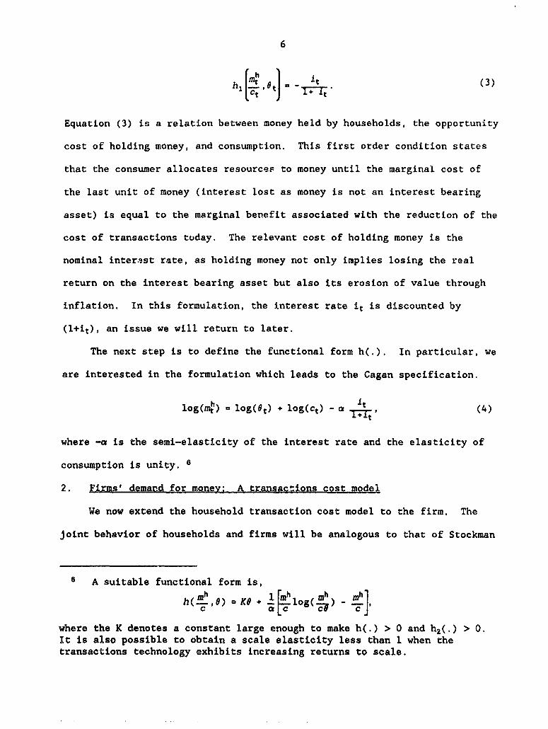
The next step is to define the functional form h(.). In particular, we

are interested in the formulation which leads to the Cagan specification.

log(mn4) a log(9t) + log(ct) - a= 4

where -a is the semi-elasticity of the interest rate and the elasticity of

consumption is unity. 6

2. Firms' demar_d for money; A transactions cost model

We now extend the household transaction cost model to the firm. The

joint behavior of households and firms will be analogous to that of Stockman

6 A suitable functional form is,

h( Ph, ) X KO + 1 hlog() ch ]

where the K denotes a constant large enough to make h(.) > 0 and h2(.) > 0.It is also possible to obtain a scale elasticity less than 1 when thetransactions technology exhibits increasing returns to scale.

7

(1981). 7

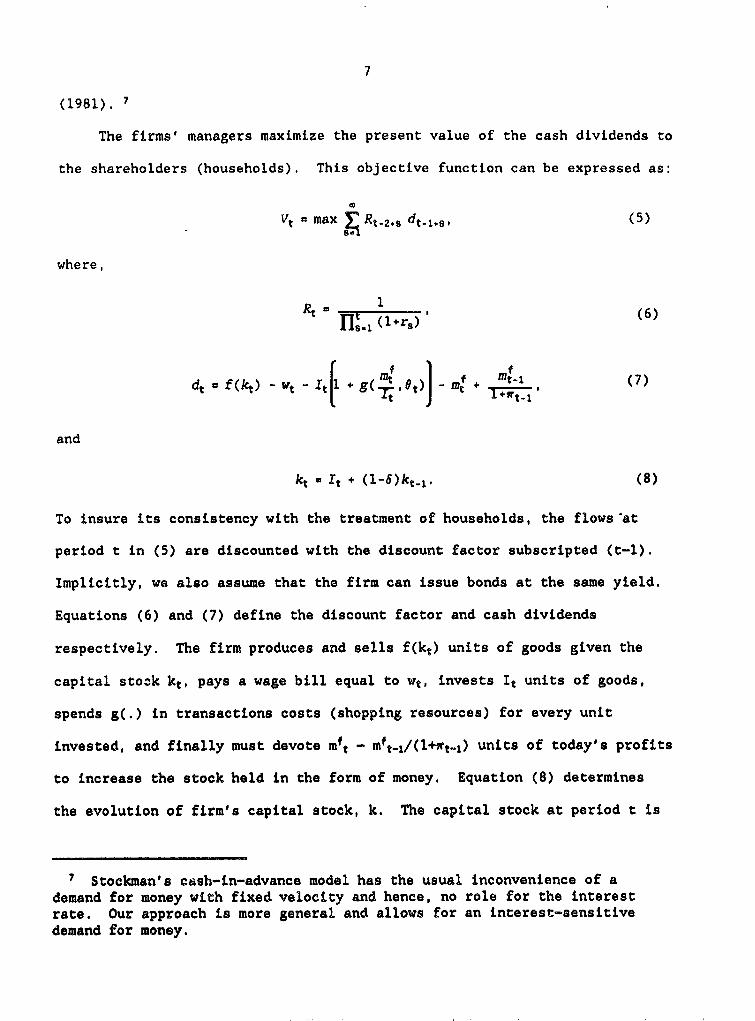
The firms' managers maximize the present value of the cash dividends to

the shareholders (households). This objective function can be expressed as:

Vt max Rt-2#s dt_1,6 , (5)

where,

Rt t r1 (6)

M n f mIt1 (7)d-t f (kt)- g( 14a):1

and

kt * It + (l-6)k-1. (8)

To insure its consistency with the treatment of households, the flows at

period t in (5) are discounted with the discount factor subscripted (t-l).

Implicitly, we also assume that the firm can issue bonds at the same yield.

Equations (6) and (7) define the discount factor and cash dividends

respectively. The firm produces and sells f(kt) units of goods given the

capital stock kt, pays a wage bill equal to wt, invests It units of goods,

spends g(.) in transactions costs (shopping resources) for every unit

invested, and finally must devote mft - mft t./(l+Wt_i) units of today's profits

to increase the stock held in the form of money. Equation (8) determines

the evolution of firm's capital stock, k. The capital stock at period t is

7 Stockman's cish-in-advance model has the usual inconvenience of ademand for money with fixed velocity and hence, no role for the interestrate. Our approach is more general and allows for an interest-sensitivedemand for money.

8

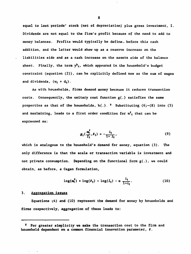
equal to last periods' stock (net of depreciation) plus gross investment, I.

Dividends are not equal to the firm's profit because of the need to add to

money balances. Profits would typically be define~. before this cash

addition, and the latter would show up as a reserve increase on the

liabilities side and as a cash increase on the assets side of the balance

sheet. Finally, the term Yht, which appeared in the household's budget

constraint (equation (2)), can be explicitly defined now as the sum of wages

and dividends, (wt + dt).

As with households, firms demand money because it reduces transaction

costs. Consequently, the unitary cost function g(.) satisfies the same

properties as that of the households, h(.). 8 Substituting (6j-(8) into (5)

and maximizing, leads to a first order condition for mft that can be

expressed as:

91( at) a -. (9)

which is analogous to the household's demand for money, equation (3). The

only difference is that the scale or transaction variable is investment and

not private consumption. Depending on the functional form g(.), we could

obtain, as before, a Cagan formulation,

f ~~~~~~~~itlog(z4) a log(Ot) + log(*T) - a . (10)

3. Aggregation issues

Equations k4) and (10) represent the demand for money by households and

firms respectively, aggregation of these leads to:

8 For greater simplicity we make the transaction cost to the firm andhousehold dependent on a common financial innovation parameter, 0.

9

log(nm) a log(O) + log(It + ct) - a (11)

To obtain (4) and (10), however, we used the simplifying assumption of

a common scale e'asticity equal to unity. However, the model can yield

money demand functions where the scale elasticities are less than one.

Aggregation in the more general case is discussed in Appendix A.

In our empirical implementation we will estimate the following

equation:

10g(nk) - 7t + f1 it + p2 log(Qt)+&t- (12)

-here it represents some measurement of ;he opportunity cost (whether it is

i or i/(l+i) will be discussed later), Qt some measurement of the scale

variable, log(et) - et, and vt is the error term introduced into (12) to have

the equation in a regression form. This error may have different sources,

some of which are discussed in Appendix A.

4. The oRRortunity cost of money

While the specifications yield i/(l+i) as the relevant opportunity cost

measure, most of the empirical literature on money demand employs i. The

difference is not trivial from the empirical point of view, as the variable

i has higher variability than i/(l+i). Further, in the case of high

inflation countries (which constitute half of our sample), the difference

between these two measures can be considerable.

In what follows, we explain why i/(l+i) is the relevant opportunity

cost variable: At the end of period t, the household must decide how much

to hold in the form of money and how much to spend on consumption. The last

unit allocated to money represents a loss of the interest rate it, a cash

flow which would be realized at the end of period (t+l). The benefit of the

10

last unit allocated to money, however, reduces the unitary cost of

consumption transactions by hj(.) at the end of period t. Consequently, to

make benefits and costs comparable at a point in time, the nominal flow it

must be discounted by the factor (l+it).

The model presented here can, with some alterations, also produce i as

the opportunity cost of holding money. The key difference in the results

rests directly on the timing of the services associated to the current money

decision. If current money decisions yield services next period (mt,, is

decided at t), i is the relevant opportunity cost variable. To illustrate

chis in the case of the consumer, we modify the budget constraint, (2), in

the following way:

bt.,1 (l+irt)mh.'i c. hllth ejct bt(l+ rt)+ h Yh (13)

where stocks and flows are now betrer understood as occurring at the

beginning of period. Now mht is a state variable and the consumer chooses ct

and mht+l at the beginning of period t. Money, therefore, must be chosen one

period before it yields transaction services. Analogous maximization to

section 2 would yield the relation,

h, [mt+^ °e ]u _it(14)

In what follows, we argue that the assumption that produces a specification

such as equation (13) does not lend itself well to application using

quarterly or lower frequency data. The beginning-of-period measurement

introduces a wedge between the time when the money decision is made (since

mht+l is chosen at time t) and the transaction services that decision

11

produces, which occur at t+l. Perhaps such time interval is less arbitrary

when the data in question are available at a frequency similar to the actual

transactions period (say one month or higher), but with quarterly data or

annual data it appears more plausible to think that decisions to consume and

hold money are made simultaneously. In the end, we conduct broad

specification searches that consider, in turn, both measures of opportunity

cost and allow the data to determine the choice.

The theoretical framework assigns a well-defined role to "financial

innovation" in the determination of money demand, indicating that its

omission would result in a misspecified relationship. In the section that

follows we illustrate the failure of approaches that ignore the role of

financial innovation. In Section IV we consider a variety of alternatives

in modeling financial innovation.

III. FAILURE OF TRADITIONAL APPROACHES

Empirical studies of money demand typically rely on a specification

such as (12) as a starting point. However, empirical applications of this

basic model have been commonly plagued by a variety of problems, among which

the more serious have been: persistent overprediction, frequently referred

to as "missing money" episodes;9 implausible parameter estimates, commonly

in the form of income elasticities well in excess of unity; and, highly

autocorrelated errors. To deal with the problem of serially correlated

errors and ir.corporate "short-run" dynamics, most commonly under the

assumption of some form of partial adjustment scheme, specifications such as

9 A period of "missing money" ocurred in Chile after 1984 where actualmoney was consistently below money demand predictions.

12

(12) are frequently extended to include a lagged dependent variable. Even

then, the basic problems tend to persist, particularly if the sample

considered covers a broad time period, thus suggesting that the traditional

model may be misspecified. As the previous section illustrates,

misspecification could arise because of failure to account explicitly for

financial innovation or, in the case of the countries where only industrial

production is available, the use of an inappropriate scale variable.

In addition to basic misspecification problems, the estimation of money

demand may be further complicated by the time series properties of the

variables themselves. The theoretical relationship among real money

balances, a scale variable, and an opportunity cost variable is most

commonly specified in terms of levels. As a consequence, empirical studies

of money demand have most often involved the estimation of a linear or log-

linear versions of (12). However, it has been commonly found that income,

interest rates, and real money balances are non-stationary processes. 10

If these variables are all individually non-stationary, lnferences about the

income and interest elasticities of money demand can only be made if a

linear combination of these variables exists that is stationary; namely, if

cointegration has been established (see, for instance, Engle and Granger

(1987)). If a cointegrating vector is found, then the error term associated

with that vector is a stationary well-defined process and ordinary least

squares (OLS) provides consistent estimates of the true parameters and

10 The most common variety of nonstationarity found in economic timeseries is integration of order one (i.e., I(1)), which implies that thedlfferenced variable is stationary (i.e., I(O)) and therefore has a well-defined, finlte variance.

13

inference-making can proceed as usual. 11 Alternatively, absence of

cointegration in a traditional money demand specification would indicate

that while a scale variable and interest rates may still be necessary for

'pinning down" the steady state demand for money-they are not sufficient.

As Section II highlights, the missing variable could be financial

innovation.

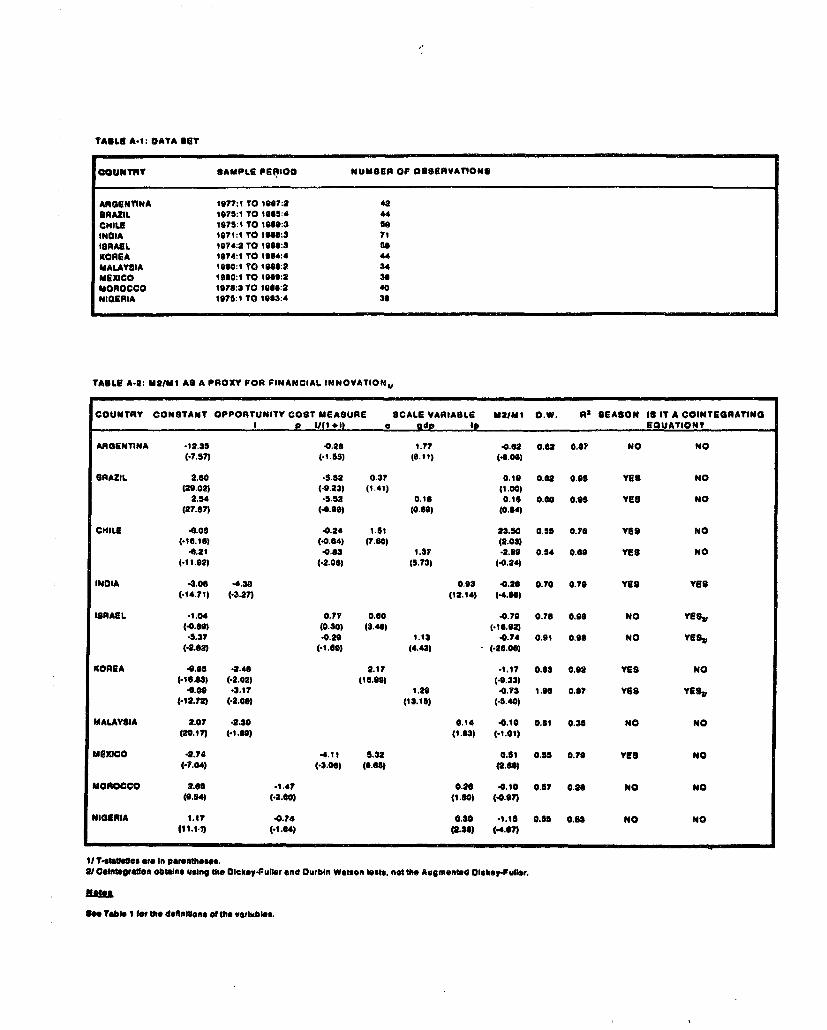
1. Data and aRecification issues

The empirical work outlined in subsequent sections employs quarterly

data for ten diverse developing countries. The sample period varies across

countries and was dictated by data availability; Table A.1 in Appendix B

details the period of coverage for each country. Real money balances are

defined as the narrow monetary aggregate, Ml, deflated by consumer prices.

When possible, quarterly time series on household consumption and GDP were

employed as scale variables. In the absence of large external imbalances,

we can expect GDP to be a good proxy for the scale variable when both firms

and households have similar transactions technology, and the government

behaves as a household when consuming and as a firm when investing. In the

other extreme, when firms are more efficient than households in making

transactions (see equation A.1 in Appendix A), we expect consumption to be a

better proxy for the scale variable. In the absence of quarterly

consumption and GDP data, industrial production was used as a proxy. 12

11 The small-sample properties of the OLS estimator when all variables areI(1) and coir.tegration obtains are examined via Monte Carlo simulations inBanerjee, et. al. (i986).

12 The countries where industrial production was the only available scalevariable (at a quarterly frequency) are: India, Malaysia, Morocco, andNigeria.

14

Real balances as well as the scale variables are expressed in per

capita terms. The quarterly population series was constructed from the

annual observations under the assumption that population growth is evenly

distributed throughout the year. Nominal interest rates on deposits were

used, when possible, as a measure of opportunity cost. For countries where

such rates were regulated and virtually constant over the sample period,

however inflation, as measured by consumer prices, was the preferred choice. 1

The theoretical model outlined in the previous section indicates that

i/(l+i) is perhaps a more appropriate measurement of opportunity cost.

Consequently, for the five high-inflation countries in our sample, where

this distinction acquires importance, all subsequent estimation uses

i/(l+i). For the relatively low inflation countries the more conventional

measure is retained, as it generally provided superior results. Seasonal

dummies were included when appropriate.

2. EmRirical results

To assess the time series properties of the variables of interest the

Dickey-Fuller test (D.F.) outlined in Dickey and Fuller (1981), and the

augmented Dickey-Fuller (A.D.F.) were employed. As is commonly the case,

the null hypothesis of a unit root in money, income, and the opportunity

cost variables could not be rejected. 14 Having thus established that the

variables in question are I(1) (unit root tests were also performed on the

differenced variables), traditional money demand specifications were

13 Inflation was used as a more relevant measure of opportunity cost inMorocco, and Nigeria.

14 The tests performed tested both the null hypothesis of a simple randomwalk as well a random walk with a constant drift. While the results ofthese tests are not reported in the paper, to economize on space, these areavailable upon request.

15

estimated by applying OLS to a variety of specifications that included

alternative sets of scale and opportunity cost variables. To test for

cointegration, the residuals of these equations were subjected to the

D.F. and A.D.F. tests making the appropriate adjustments in the critical

values (see Engle and Yoo (1987)).

The results summarized in Table 1 have a number of common

characteristics worth noting. With the exception of Israel, the scale and

opportunity cost variables have the anticipated signs, However, the

magnitudes of several elasticity estimates lack economic meaning (for

instance, Mexico and Argentina). 15 The Durbin-Watson (D.W.) statistics

are uniformly low. In many previous studies of money demand the low

D.W. statistics were taken as evidence that portfolio changes occurred

gradually, and a partial adjustment schenme was warranted (for surveys see

Goldfeld and Sichel (1990) and Judd and Scadding (1982)). More recently,

the D.W. statistic has been reinterpreted as yet another way of assessing

whether individual variables are stationary (Bhargava (1986)) or whether a

cointegrating vector has been found (Engle and Granger (1987)). Thus, the

low D.W. of these traditional money demand equations are consistent with the

D.F. and A.D.F. test results on the residuals which indicate that with the

exception of India and Korea, the null hypothesis of no cointegration cannot

be rejected. 16 The lack of cointegration in the remaining eight

countries, irrespective of which scale variable or opportunity cost variable

was used, may be a product of the low power of these tests when the

15 This is a different result from that of Melnick (1989), who findscointegration in the case of Argentina during the 1978-85 period.

16 In the case of Korea the test results are mixed. The D.W. and D.F.tests indicate cointegration but the A.D.F. does not.

16

autocorrelation coefficient is close to one. 17 An equally plausible and

perhaps more probable explanation is that traditional specifications

routinely fail to account for the ongoing process of financial innovation.

To the extent that the financial innovation process has any Rgrmgnent

effects on desired money holdings, specifications such as those presented in

Table 1 would be misspecified and not expected to cointegrate.

IV. THE EXTENDED MODEL: ALTERNATIVE APPROACHES TO MODELLING

FINANCIAL INNOVATION

The arguments in favor of incorporating a role for financial innovation

or technological change in the demand for money have long been considered in

the money demand literature. Gurley and Shaw (1955 and 1960), argued that

the creation and growth of money substitutes made the demand for money more

interest elastic. Lieberman (1977), argues that increased use of credit,

better synchronization of receipts and expenditures, reduced mail float,

more intensive use of money substitutes, and more efficient payments

mechanisms will tend to permanently decrease the transaction demand for

money over time. Estimating the demand for narrow money in the United

States, Lieberman incorporates a time trend in the money demand equation as

a proxy for the unobservable variable-technological change. More recently,

Ochs and Rush (1983), focusing on the demand for currency, argue that once

innovations that economize on the use of currency have taken place, the

impact on the demand for currency is likely to be permanent since these

innovations require long-lived capital investments with very substantial

17 If the error terms are stationary but highly autocorrelated and thenumber of observations are small these tests would = rejectnonstationarity a high proportion of the time.

17

sunk costs but low operating costs. In similar spirit Moore, Porter and

Small (1988), include a time trend in the "long-run" demand for Ml in the

United States.

Despite empirical evidence from the industrial countries supporting

inclusion of a financial innovation proxy in the demand for money, most of

the literature does not rely on such a specification for developing

countries where there is also evidence of money demand instability.

Evidence of instability is to be found in the work of Darrat (1986), who

tests the stability of money demand for four Latin American countries; in

Sundararajan and Balifio (1990), who test for and find shifts in money demand

in several developing countries during periods of banking crises; and in

Rossi (1989), who identifies a downward shift in the demand for money during

the 1980s for Brazil. Exceptions to this neglect of the impact of financial

innovation on money demand are Darrat and Webb (1986), who test the Gurley-

Shaw thesis for India, and Arrau and De Gregorio (1991), who model financial

innovation via a time-varying intercept for Chile and Kexico: this approach

is used later. In the sections that follow the demand for money is

reestimated by considering a variety of proxies for financial innovation.

1. Is a deterministic trend a good proxy for financial innovation?

To the extent that financial innovation can be characterized by fairly

smooth improvements in cash management techniques, a negative time trend

would appear to be a reasonable proxy. Equation (12), with the relevant

variations in scale and opportunity cost variables was estimated for all the

countries in the sample and the results are summarized in Table 2, where the

choice of variables is also detailed.

18

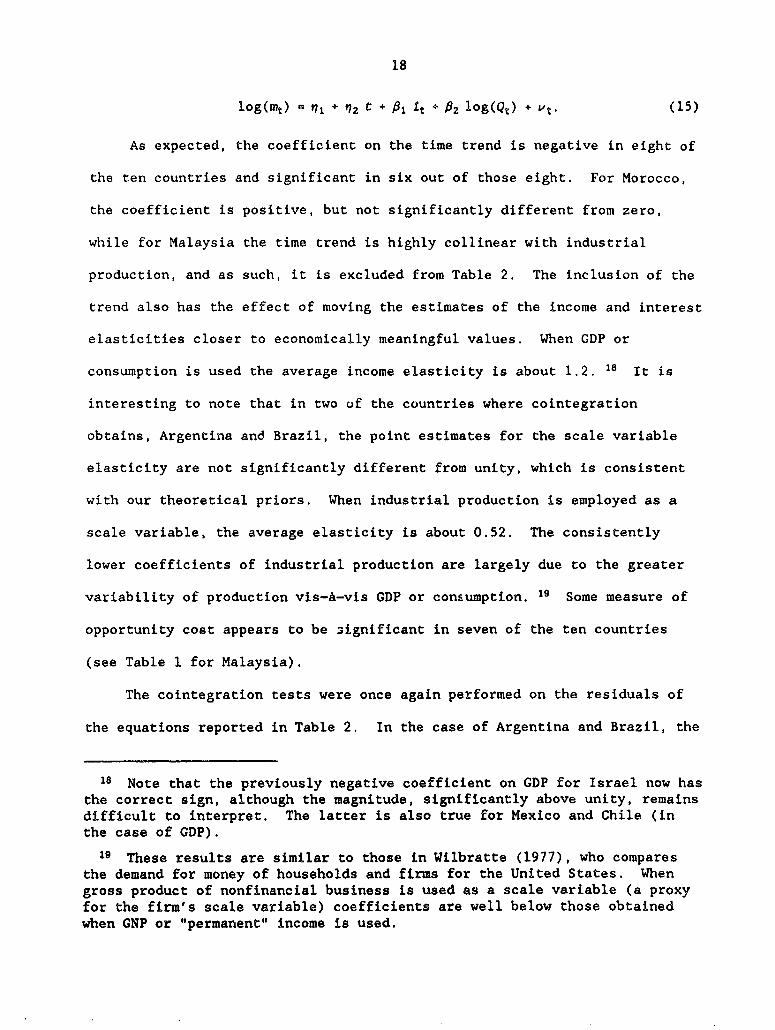
10og(mt) n71 + '72 t + 1 1t + 02 log(Q) + vt. (15)

As expected, the coefficient on the time trend is negative in eight of

the ten countries and significant in six out of those eight. For Morocco,

the coefficient is positive, but not significantly different from zero,

while for Malaysia the time trend is highly collinear with industrial

production, and as such, it is excluded from Table 2. The inclusion of the

trend also has the effect of moving the estimates of the income and interest

elasticities closer to economically meaningful values. When GDP or

consumption is used the average income elasticity is about 1.2. 18 It is

interesting to note that in two of the countries where cointegration

obtains, Argentina and Brazil, the point estimates for the scale variable

elasticity are not significantly different from unity, which is consistent

with our theoretical priors. When industrial production is employed as a

scale variable, the average elasticity is about 0.52. The consistently

lower coefficients of industrial production are largely due to the greater

variability of production vis-a-vis GDP or consumption. 19 Some measure of

opportunity cost appears to be 3ignificant in seven of the ten countries

(see Table 1 for Malaysia).

The cointegration tests were once again performed on the residuals of

the equations reported in Table 2. In the case of Argentina and Brazil, the

18 Note that the previously negative coefficient on GDP for Israel now hasthe correct sign, although the magnitude, significantly above unity, remainsdifficult to interpret. The latter is also true for Mexico and Chile (inthe case of GDP).

19 These results are similar to those in Wilbratte (1977), who comparesthe demand for money of households and firms for the United States. Whengross product of nonfinancial business is used as a scale variable (a proxyfor the firm's scale variable) coefficients are well below those obtainedwhen GNP or "permanent" income is used.

19

inclusion of the time trend had the effect of making the residuals

stationary-that is, cointegration was achieved. In the case of India,

cointegration obtains with and without a time trend, while in the case of

Korea, where a traditional money demand equation did not appear to be

misspecified, the inclusion of the time trend increased the serial

correlation in the errors. In the remaining six countries, with no

cointegrating vector, it would appear the financial innovation process

cannot be adequately proxied by a deterministic trend.

The log of the ratio of M2 to Ml was also used as a proxy for financial

innovation. The rationale is that the greater the array of money

substitutes (reflected in the quasi-money component of M2) the lower the

demand for narrow money. The results, presented in Table A-2 in Appendix B,

indicate that in eight of the ten countries M2/Ml had the anticipated sign.

In the case of Korea and Israel, the inclusion of M2/Ml produced a

cointegrating vector.20 However in most instances, M2/Ml was found to be

collinear with the opportunity cost variable, as such, less weight is given

to these results. In the section that follows financial innovation is

modelled as a stochastic trend.

2. Is a stochastic trend a good proxy for financial innovation?

This section presents an alternative approach to deal with financial

innovation. We assume that technological changes in transactions (financial

innovation) can be described by a stochastic trend process, and therefore

they are permanent shocks to money demand. As in Arrau and De Gregorio

(1991), the assumption is that the technological parameter evolves as the

20 In the case of Israel, this specification also yielded plausible valuesfor the income (and consumption) elasticities.

20

simplest stochastic trend process, a random walk. It is also assumed that

the permanent shocks are orthogonal to the stationary shocks affecting money

demand.

These assumptions can be written as:

't e7t-1 4 Et (16)

where,

et-N(O,u2), and cov(et,vt)uO. (17)

We also define ui - yo2 and a2 - (1-")U2, where the parameter I represents

the relative importance of the permanent shocks (financial innovation) to

money demand vis-&-vis the transitory shocks.

Therefore, the demand for money becomes:

l0g(Md) - t - 1 It P a2 log(Q1 ) + vt, (18)

which is a standard regression equation except that the intercept evolves as

a random walk.

Note that this definition for financial innovation is "everything that

affects permanently the demand for money other than the scale and

opportunity cost variables." Therefore, it may include other permanent

changes besides pure technology. For example, permanent changes in

regulatory policy that affect the banking system's ability to provide the

medium of exchange would be included in our estimation of financial

innovation. This would explain why periods of "negative innovations" can be

observed. Other sources of permanent shocks could also be included, as for

example, people's expectations about policies that affect the costs of

holding money. It is beyond the scope of this paper to disentangle the

21

different explanations for permanent shifts in money demand, so we associate

all such effects in our broad concept of financial innovation.

The estimation technique employed here was first applied by Cooley and

Prescott (1973a,b, 1976) and a brief outline of it appears in Appendix B.

This three-step procedure, which allows for a time-varying intercept,

provides estimates for: the time-invariant parameters, here the elasticities

of the scale and opportunity cost variables as well as the seasonal factors;

the relative importance of the permanent shocks (financial innovation) to

money demand (i.e., e); the sequence (tt), which traces the whole path of

financial innovation and; the variance-covariance matrix of the residuals.

When 7 - 1, only permanent shocks appear in the money demand equation.

In this case, all changes in money demand are due to financial innovation.

The estimation of this case is equivalent to estimating equation (12) in

first differences. On the other extreme, y - 0 implies that qt is a

constant and OLS applied to equation (12) in levels would be the appropriate

method.

The preferred specifications for each country are shown in Table 3.

Two equations are reported by country, the first one is for the maximum

likelihood estimator of y while the second uses a value for I which is

30 percent smaller than the maximum likelihood estimate. This alternative

is presented because, as shown in Arrau and De Gregorio (1991) with Monte

Carlo simulations, misspecification of the true process followed by et and ut

may produce an upward bias in the estimation of 7.

India is the only country where the assumption of a time-varying

intercept did not produce reasonable results. This, however, is not

22

surprising since the cointegration results of the traditional specifications

indicate that there was no nonstationary variable omitted.

The method used in this section provides quite a good fit. The reason

for this is that it allows maximum flexibility (through the choice of nt) in

explaining the behavior of the dependent variable. In the extreme case that

y-1, the R2 is equal to 1, since all the residual is identified with

financial innovation. In the regressions reported in Table 3 the R2 are, in

general, above 0.98. Under a correct specification of this model we also

obtain unbiased estimates of the elasticities of the scale and opportunity

cost variables. The tight fit, however, does not imply that money demand

can be forecast with precision, since the change in ,t can not be forecast,

and these changes can have a large variance.

There are no clear cut criteria to evaluate whether or not a time-

varying intercept is a reasonable assumption, as in the case where a time

trend or M2/M1 is used as a proxy for financial innovation, there the first

test is to establish whether the inclusion produces cointegration. In any

event, the estimations presented in Table 3 show that except for Malaysia

and Nigeria, where the income elasticities are not significant, the

parameter estimates fall in line with economic priors. As discussed

previously, the problem with Malaysia and Nigeria may be the use of

industrial production as a "proxy" of the true scale variable. Income

elasticities fluctuate between 0.2 and 1, which are consistent not only in

sign but also in magnitude with our theoretical presumptions. Thus, one of

the traditional anomalies of money demand estimations, income elasticities

larger than one, is not present in these estimations. Except for Argentina,

consumption perforus better than GDP as a scale variable when both variables

23

where available. Interest rate elasticities range from -0.2 to -3.1, which

are also in the feasible range. Although, for some countries, the value of

the interest rate elasticity is statistically insignificant.

Comparing the estimations with those that are analogous when a

deterministic trend is used, it is observed that in most cases the

elasticities are smaller, in absolute value, under the assumption that the

intercept is stochastic. Another important result is that whenever the

deterministic time trend was included with a time varying intercept, the

former never appears to be significant. 21 This suggests that one, but not

both, can be used to approximate financial innovation. This, in turn,

suggests that when financial innovation is modeled as a random walk, the

process does not have a drift. Table 4 suwmmarizes the choice of variables

and estimation technique that gave the best results.

3. Is the role of financial innovation lar&e or_smal

After using several alternatives to estimate financial innovation, it

is useful to discuss quantitatively how important its effects on the demand

for money are. We present two basic approaches. The first one consists of

looking at the value of y. This measure tells us how much of the

(unexplained) shocks to money demand are due to financial innovation. The

second one is to look at the role of financial innovation in the exRlaingd

variation of money demand. For this purpose some variance decompositions

are performed.

21 This is consistent with the results of Monte Carlo simulationspresented in Cooley and Prescott (1973b), which indicate it isobservationally difficult to distinguish a time trend and a time varyingintercept with OLS. Using a time varying intercept, however, is moresuccessful in identifying the presence of time trends.

24

The maximum likelihood estimations of y show that its value is quite

large in all the countries. For the cases of Argentina, Israel and Mexico

the maximum likelihood estimation of I was at the extreme value of 1. For

the rest of the countries, the value of y is higher than 0.66. This implies

that more than 2/3 of the variance of the total residual in the money demand

equation is accounted for by financial innovation. In other words, most of

the shocks to money demand have permanent effects.

It is interesting to note that in the high inflation countries, the

value of 7 is larger than in low-to-moderate inflation countries. Figure 1

illustrates in a scatterplot between 7 and average inflation this positive

correlation. In fact, the three countries where 7 is one have been

characterized by high inflation during the sample period. This would seem

to indicate that the shocks to money demand have a larger permanent

component in high inflation countries. This result, is in part due to our

broad definition of financial innovation, which is also capturing the

secular "dollarization" that has taken place in most of the high inflation

countries in our sample. 2 However, this is not the only way to quantify

the importance of financial innovation on changes in money demand. We

should also compare its explanatory power with respect to the other

regressors, an issue that is addressed in what follows.

The next way of evaluating the importance of financial innovation in

money demand is to determine how much of the explained variation in money

demand is due to financial innovation vis-&-vis its traditional

2 To isolate the effects of currency substitution from financialinnovation a money demand function, such as the one derived in Guidotti(1989), would have to be estimated. There, a foreign interest rate affectsthe demand for money in addition to the domestic rate, the scale variable,and the financial technology parameter.

25

determinants. Although it was found that a time trend does not wholly

capture the financial innovation process in the majority of the countries,

it is still useful to investigate what share of the explained variation in

money demand is traced to this proxy of technological change. Let us

consider the case where a time trend is included in the demAand for money and

define m as the fitted value of m. The ga=lp variance of m can be

decomposed as follows:

Var(m't) = #12Var(1t) + 2

2Var(log(Qt)) + j 32 Var(t) + Covs, (19)

where Covs represents the sum of the three covariances (appropriately

weighed by the nj's). Equation (12) can be used to approximate a variance

decomposition. We consider that the relative explanatory power of each term

in the total variance is the share of the variance in the total variance

discounted by the covariance terms. This is equivalent to assuming that the

covariances are proportionately distributed according to these shares.

Three remarks are worth emphasizing with respect to this procedure.

First, this decomposition is conditional on a given sample, since variables

with unit roots, as is the case with the variables in our data set, have

infinite unconditional variance. For this same reason the sample variance

of time is considered. Although the trend is a deterministic variable, it

has variation in the sample and contributes to the variance of m*. Finally,

as most variance decompositions, the estimates of 's are treated as the

true values of the parameters, without considering their own variance.

Table 5 presents this variance decomposition. Two striking results

emerge. First, the time trend accounts for an average of 68 percent of the

explained variation in the high inflation countries (Argentina, Brazil,

Israel, and Mexico) while accounting for only 14 percent in the remaining

26

six moderate-to-low inflation countries. Second, in three of the four high

inflation countries (Brazil, Israel, and Mexico), the opportunity cost

variable accounts for a higher percentage of the explained variance than the

scale variable-the opposite being true in the low-to-moderate inflation

countries (see Figure 2). The first of these observations lends support to

the view that high inflation speeds the process of financial innovation, as

ways to economize on the use of cash balances are more intensively sought.

In the case that financial innovation is modeled as a stochastic

process, the last remark made for the time trend case is quite relevant.

The estimated path of nt has two sources of variability, first the variance

of the true ,'s and second the variance of the estimators. Because we

assume that the estimates of the 's are nonstochastic and equal to their

true value, we should discount the first component in the variance

decomposition. Hence, when computing m° at t we should consider nt-, as

known and non random, therefore the variability explained by financial

innovation is the variability explained by the shock et. Thus, the

counterpart to equation (20) for the case of stochastic financial innovation

is:

Var(mwt) _ A 12 Var(It) + 2

2Var(log(Qt)) + j'2 + Covs, (20)

The rest of the procedure is analogous to the one used for the deterministic

time trend case. Columns (5) to (7) of Table 5 present the results of the

variar.e decompositions exercise in the case of the stochastic trend. The

results show that, except for Brazil, financial innovation is a very

important component of the variability of the fitted value of m. The

results are, however, not as striking as those of the previous three

columns, in fact, there is no observed clear correlation between the

27

explanatory power of financial innovation and inflation (see Figure 3). The

difference with column (1) is that although the estimate of y is larger in

inflationary countries, the estimate of a is larger in low inflation

countries. Therefore, since as was already pointed out, this method tends

to produce an almost perfect fit, the variance decomposition will assign a

larger share for financial innovation in countries that started with a very

poor fit. These include, for example, the cases of Malaysia, Morocco and

Nigeria, in which R2 in the equations without proxying financial innovation

(Table 1) are on average 0.26, due in large part to a bad proxy for the

scale variable. In contrast, in Argentina, Brazil, Israel, and Mexico the

average (for the relevant equations) is 0.78.

The results of this section highlight that in all countries,

irrespective of how it is modelled, financial innovation plays a

quantitatively important role in determining money demand and its

fluctuations. Although the evidence is less definite, among other reasons,

because the number of countries examined is too small to obtain strong

patterns, it can also be concluded that the importance of financial

innovation in explaining shocks to money demand as well as its variability

is increasing with the rate of inflation.

V. CONCLUDING REMARKS

This paper has revisited the question of the appropriate specification

of money demand functions, with a primary focus on developing countries. It

was pointed out that the transmission mechanism for monetary and fiscal

policy in a variety of economic models depends on the stability and

predictability of the demand for money. Nevertheless, empirical work done

28

by others, as well as that presented herein, indicate that traditional

approaches tend to suffer from a number of problems which suggest

misspecification.

We see two principal contributions in the present paper. First, by

examining theoretical models of the demand for money by firms as well as

households we find that the scale variable is likely to be different between

the two sectors. Thus, in estimating the aggregate demand for money the

appropriate scale variable may well depend on the relative size of each

sector's holdings of money balances, which in turn can depend on the

transactions "technology" and possible differences between the sectors in

efficiently utilizing the technology. Second, observed shifts, or movements

over time, in money holdings which are often difficult to account for

satisfactorily may be attributable to shifts or movements in the

transactions technology. By this, we mean firms and households finding ways

and/or being offered means to economize on money holdings, a process usually

referred to as "financial innovation".

In the empirical section of the paper, we examined the time series

properties of data drawn from a sample of developing countries and found

that the key variables are generally not stationary, or more precisely, they

are not integrated of order zero. Having established this fact, the

analysis proceeded to test for cointegration which, if established,

determines that the variables have a well-determined relationship to one

another. Despite the use of a variety of specifications, cointegration was

established in a minority of cases, and, where cointegration did not obtain,

the parameter estimates suggested continuing misspecification.

29

As it was posited that the above results could be the result of

ignoring the role of financial innovation, the paper then examined how such

a process could be introduced into estimation procedures. Considered first

was the possibility of modeling financial innovation as a deterministic

drift process, or in other words, incorporating a time trend into

regressions. In general the results of incorporating a time trend were

favorable in terms of a significant parameter for the trend itself.

However, despite obtaining more plausible parameter estimates for the other

explanatory variables, in six of the ten countries examined the continued

lack of a cointegrating vector suggested that a time trend was not an

adequate proxy for financial innovation. An alternative proxy variable, the

ratio of Ml to M2, was also considered, but the results were even less

clearcut. We then considered whether financial innovation could be modeled

as permanent shocks to money demand by assuming that the technological or

innovation process follows a random walk. In general, the results were

again an improvement in terms of deriving time-invariant parameters of the

money demand function, and indeed better than modeling innovation as a time

trend.

Consideration was then given to ascertaining how important financial

innovation is in determining the demand for money. We found that, in the

sample of developing countries chosen, the role of financial innovation

(however modeled) was quantitatively important in determining money demand.

It was also established that, although the sample was relatively small,

there seems to be a positive relationship between the importance of

financial innovation and the average rate of inflation that a country is

experiencing. This finding is consistent with the prior that the costs of

3.)

failing to innovate will be higher as the inflation rate rises. Whether or

not this process is reversible and a reduction in average inflation reduces

the importance of financial innovation for a given country is an open

question.

The findings of the paper suggest that while it may be difficult to

forecast the path of financial innovation, it may well be beneficial to

model the process in some way, so as to recover better estimates of the

deeper parameters in the money demand function. Failure to do so may lead

to such policy difficulties as misreading the path and speed of policy

transmission, financial programming errors, and incorrect estimates (with

fiscal implications) as to seigniorage yields.

31

Appendix A: Discuss1on on Aggregation and the Regression Error

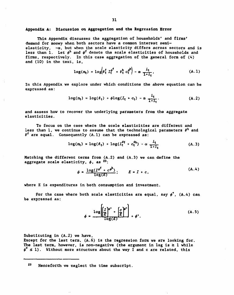
This Appendix discusses the aggregation of households' and firms'demand for money when both sectors have a common interest semi-elasticity, -a, but when the scale elasticity differs across sectors and isless than 1. Let oh and of denote the scale elasticities of households andfirms, respectively. In this case aggregation of the general form of (4)and (10) in the text, is,

log(ot) 0 0k lof + oh ch) _ 'a it (A.1)

In this Appendix we explore under which conditions the above equation can beexpressed as:

log(mn) log(et) + 4log(It + Ct) - a it (A.2)

and assess how to recover the underlying parameters from the aggregateelasticities.

To focus on the case where the scale elasticities are different andless than 1, we continue to assume that the technological parameters oh andOf are equal. Consequently (A.l) can be expressed as:

log(mt) = log(Ot) + log(I4 C c) - a = (A.3)

Matching the dlfferent terms from (A.2) and (A.3) we can define theaggregate scale elasticity, 0, as 23:

a log(I f c O); E Ilc, (A.4)

where E is expenditures in both consumption and investment.

For the case where both scale elasticities are equal, say 0*, (A.4) canbe expressed as:

log + [EC |. (A.5)

Substituting in (A.2) we have,Except for the last term, (A.6) is the regression form we are looking for.The last term, however, is non-negative (the argument in log is 2 1 while

:* 1). Without more structure about the way I and c are related, this

23 Henceforth we neglect the time subscript.

32

log(mt) a log(0t) +01log(It+Ct)- it logl' +[ ' (A.6)

term will part of the regression error and is assumed to be homoscedastic

and uncorrelated. The mean of this term will affect the level of the

intercept (log(GO) for a sample from t - 0,..,T, if the intercept is time-

varying), but not the other elasticities.

When the elasticities are not equal, however, we cannot express the

term *log(E) as homogenous of degree 1 in log(E) for the case of

proportional increases in consumption and investment (unlike A.5 above).

This means that the aggregate elasticity is not invariant with respect to

the level of E (for proportional increase in consumption and investment) and

therefore (A.2) is not a suitable regression equation. The intuition behind

this result is that with different scale elasticities, that is with

different scale economies associated to the transaction technologies from

households and firms, proportional increases in both scale variables have

different proportional increases in their respective money demands, so that

we cannot make the aggregate elasticity independent of the individual

levels.

In short, we conclude that to obtain a regression equation like (A.2)

we need to make both transaction functions g(.) and h(.) identical. If the

scale elasticities are equal to unity, the regression error is not due to

aggregation problems but stem from other sources (e.g. measurement errors).

However, in the case where scale elasticities are equal but less than 1, a

regression error, which stems from aggregation, appears.

TAILe A-I: DATA SET

COUNTRY SAMPLE PERIOD NUMBER OF OSSERVATIONS

ARGENTINA 1977:t TO 1987:2 48BRAZIL 1975:1 TO 1965:4 44CHILE 1975:1 TO 1t89:3 SoINDIA 1071:1 TO 1961:3 IsISRAEL 1974:2 TO 1968:3 D9KOREA 1974:1 TO ¶084:4 44MALAYSIA 10,1:1 TO 1986:2 34MEXICO 1060:1 TO 1089:2 36MOROCCO 1907:3 TO 1984:2 40NIGERIA 1975:1 TO 1903:4 36

TABLE A-2: M2IMI AS A PROXY FOR FINANCIAL INNOVATION,

COUNTRY CONSTANT OPPORTUNITY COST MEASURE SCALE VARIABLE M21AI O.W. AS SEASON IS IT A COINTEGRATINGI P U(I+1) a ado Ip EQUATION?

ARGENTINA *12.35 .0.26 1.77 40.62 0.62 0.67 NO NO(-7.57) (-1.55) (6.11 (4.06)

BRAZIL 2.60 *5.S2 0.37 0.19 0.62 0.95 YES NO(29.02) (-0.23) (1.41) (1.00)

2.54 *s.5sa C.li 0.1 0.60 0.85 YES NO(27.57) (4.00) (0.69) (0.64)

CHILE 4.05 4.24 1.51 23.50 0.55 0.76 YES NO(.16.16) (4.64) (7.60) (2.03)

4.21 -0.63 1.37 -2.69 0.54 0.69 YES NO(. 1.02) (-2.06) (5.73) (4.24)

INOIA 4.08 -4.38 0.93 4.26 0.70 0.70 YES YES(.4.71) (-3.27) (12.14) (-4.96)

ISRAEL .1.04 0.77 0.60 4.79 0.76 0.96 NO YES,(4.60) (0.30) (3.46) (416.02)*5.37 40.29 1.13 40.74 0.91 0.90 NO YES3

(-2.82) (1.60) (4.42) (-26.00)

KOREA 4.96 -2.48 2.17 -1.17 0.63 0.02 YES NO(-16.63) (-2.02) (6.00) (-0.33)

4.00 43.17 1.29 4.73 1.06 0.67 YES YESt-12.72) (-2.00) (13.16) (-5.40)

MALAYSIA 2.07 .2.30 0.14 -0.10 0.61 0.36 NO NO(20-17) (. (1.3) -1.01)

MEXICO *2.74 4.11 5.32 0.61 0.65 0.76 YES NO(-7.04) (-3.08) (6.6) (2.61)

MOROCCO 2.65 -1.47 0.20 -0.10 0.67 0.29 NO NO(6.14) (-2.40) (1.60) (4.07)

NIlGIA 1.17 -0.74 0.30 *1.10 0.56 o.6a NO NO(11.14) (*e.14) (2.38) (4.67)

1/ T-tagelas *re In parentheses.21 Cotegraon ObtWne ugIna the Olokep-Fuler and Ourbin Watson tests, not the Augmented Olokey-Fuller.

Oft Table I fet Me definition of the vaeIabIes.

34

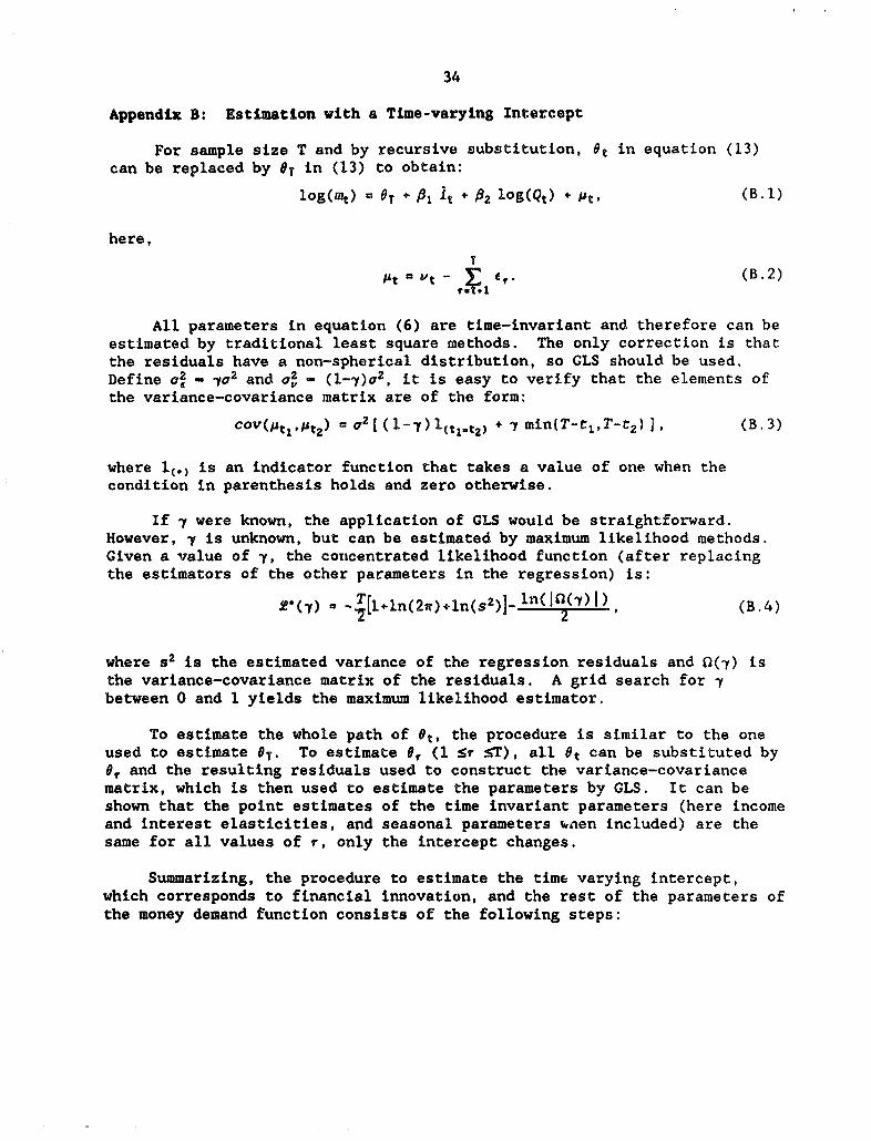
Appendix B: Estimation with a Time-varying Intercept

For sample size T and by recursive substitution, Ot in equation (13)can be replaced by PT in (13) to obtain:

log(m) a 9T 4 it log(Q9) Pt' (B.l)

here,T

M't - E. (B.2)

All parameters in equation (6) are time-invariant and therefore can beestimated by traditional least square methods. The only correction is thatthe residuals have a non-spherical distribution, so GLS should be used.Define a2 - YO2 and o2 - (1-)g2, it is easy to verify that the elements ofthe variance-covariance matrix are of the form:

COV(At1At2) -a v2[ (1-7) 1tlt 2) + -y min(T-t1 ,T-t2)], (B.3)

where 1(.) is an indicator function that takes a value of one when thecondition in parenthesis holds and zero otherwise.

If -y were known, the application of GLS would be straightforward.However, 7 is unknown, but can be estimated by maximum likelihood methods.Given a value of y, the concentrated likelihood function (after replacingthe estimators of the other parameters in the regression) is:

(7) T[l+ln(2t)+ln(S2)]- ln(1In(z) I) (B.4)

where s2 is the estimated variance of the regression residuals and 0(z) isthe variance-covariance matrix of the residuals. A grid search for -between 0 and 1 yields the maximum likelihood estimator.

To estimate the whole path of °t. the procedure is similar to the oneused to estimate 9 T. To estimate 0, (1 Sr ST), all Pt can be substituted by°, and the resulting residuals used to construct the variance-covariancematrix, which is then used to estimate the parameters by GLS. It can beshown that the point estimates of the time invariant parameters (here incomeand interest elasticities, and seasonal parameters unen included) are thesame for all values of r, only the intercept changes.

Summarizing, the procedure to estimate the time varying intercept,which corresponds to financial innovation, and the rest of the parameters of

the money demand function consists of the following steps:

35

(i) Estimation of equation (6) by GLS for all y in [0,1].

(ii) Choice of the 7 that maximizes the concentrated likelihood. 24

This stage also provides the estimators of the time invariantparameters.

(iii) Recovering the whole path of Ot by estimating, with GLS, anequation similar (6) with 6, as intercept for all r.

24 Note that the estimation of y is for the equation with eT as theintercept. This could be done for other values of the intercept, but theresults do not change significantly.

36

REFERENCES

Arrau, Patricio and Jos6 De Gregorio, "Financial Innovation and MoneyDemand: Theory and Empirical Implementation," Working Paper No. 585,World Bank, (1991).

Bhargava, A., "On the Theory of Testing for Unit Roots in Observed TimeSeries," Reviw of Economic Studes, (1986), pp. 369-384.

Cagan, P., "The Dynamics of Hyper-Inflation", in M. Friedman (ed.)Studip of the Ouantity Theory of Money, Chicago: Chicago UniversityPress, (1956).

Cooley, T.F. and E. Prescott, "An Adaptive Regression Model," IntgernationalEconomic Review, (1973a), pp. 364-371.

, "Test of an Adaptive Regression Model," Revieof Economics and Statistics, (1973b), pp. 248-256.

, "Estimation in the Presence of StochasticParameter Variation," E£onomtXic-a, (1976), pp. 167-184.

Darrat, Ali F., "Monetization and Stability of Money Demand in DevelopingCountries: The Latin American Case," Savines and Development, (1986),pp. 59-72.

Darrat, Ali F. and Michael A. Webb, "Financial Changes and InterestElasticity of Money Demand: Further Tests of the Gurley Shaw Thesis,"Jounual of DeveloDment Studies, (1986), pp. 724-730.

De Gregorio, Jos6, "Welfare Costr of Inflation, Seignorage, and FinancialInnovation," IMF Working Paper Number WP/91/1, (1991).

Dickey D.A. and W.A. Fuller, "Likelihood Ratio Statistics for AutoregressiveTime Series with a Unit Root," Econ2metrica, (1981), pp. 1057-1072.

Engle, Robert F. and C.W.J. Granger, "Co-integration and Error Correction:Representation, Estimation, and Testing," Econometrica, (1987),pp. 251-276.

Engle, Robert F. and B.S. Yoo, "Forecasting and Testing Co-integratedSystems," Journal f Econometrics, (1987), pp. 143-159.

Goldfeld, Stephen H., "The Case of Missing Money," Brookings Papers onEconoMic Activity, (1976), pp. 633-730.

Goldfeld, Stephen M. and Daniel E. Sichel, "The Demand for Money," in B.Friedman and F. Hanhn, (eds.) Handbook of Monetary Economigs, Vol. I,(1990).

37

Guidotti, P.E., "Currency Substitution and Financial Innovation," IMFWorking Paper WP/89/39, (1989).

Hendry, D.F. and G.E. Mizon, "Serial Correlation as a ConvenientSimplification, Not a Nuisance: A Comment on a Study of the Demand forMoney by the Bank of England," EgonomLc Journal, (1978), pp. 549-563.

Judd, John P. and John L. Scadding, "The Search for a Stable Money DemandFunction," Josnal of Economic Literature, (1982), pp. 993-1023.

Lieberman, Charles, "The Transaction Demand for Money and TechnologicalChange," Review of Economics and Statistics, (1977), pp. 307-317.

Melnick, Rafi, "The Demand for Money in Argentina 1978-87: Before and afterthe Austral Program," mimeo, (1989).

Moore, George R., Richard Porter, and David H. Small, "Modelling theDisaggregated Demand for M2 and Ml: The U.S. Experience in the 1980s,"in Board of Governors of the Federal Reserve System, Financial Sectorsin Open Economies: Empirical Analysis and Policy Issues, (Washington:Board of Governors), (1990).

Ochs, Jack and Mark Rush, "The Persistence of Interest-Rate Effects on theDemand for Currency," Journal of Money Credit and Banking, (1983),pp.499-505.

Rossi, Jose W., "The Demand for Money in Brazil: What Happened in the1980s," JournAl of Develogment Economics, (1989), pp. 357-367.

Stockman, A. C., "Anticipated Inflation and the Capital Stock in aCash-in-Advance Economy", Journal of Monetary Economics 8, (1981),pp. 387-393.

Sundararajan, V. and TomiAs J.T. Baliftio, "Issues in Recent Banking Crises inDeveloping Countries," IMF Working Paper Number WP/90/19, (1990).

Wilbratte, Barry J., "Some Essential Differences in the Demand for Money byHouseholds and by Firms," Journal of Finance, (1977), pp. 1091-1099.

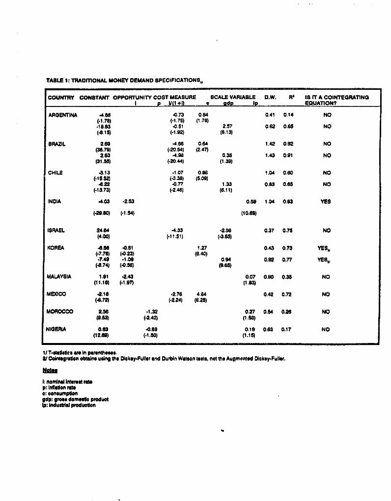
TABLE 1: TRADMONAL MONEY DEMiAND SPECIFICATIONSU

COUNTRY CONSTANT OPPORTUNITY COST MEASURE SCALE VARIABLE D.W. R' 18 rr A COINnERATING_eI p /(1 +Q a - dp IG EOUATION?

AGENTINA .4.86 40.73 0.84 0.41 0.14 NO(.1.78) (.1.75) (1.76)*18.83 .0.51 2.57 0.62 0.65 NO(4.15) (1. (8.13)

BRAZIL 2.69 .4.86 0.64 1.42 0.92 NO(36.79) (-20.54) (2.47)

2.63 4.98 0.35 1.43 0.91 NO(31.55) (.20.44) (1.39)

CHILE J5.13 *1.07 0.96 1.04 0.60 NO(.15.52) (-3.38) (5.09)

4.22 .0.77 1.33 0.83 0.65 NO(.13.73) (-2.48) (6.11)

INDIA 4.03 *2.53 0.59 1.04 0.63 YES

(.29.80) (.1.54) (10.

ISPAEL 24.64 *4.33 *2.98 0.37 0.75 NO(4.00) (.1 1.51) (46M)

KOREA 4.56 4.051 1.27 0.43 0.73 YES,(.7.76) (40.23) (8.40)*7.49 *1.09 0.94 0.92 0.77 YES,

(8.74) (.0.56) (9.

MALAYSIA 1.91 *2.43 0.07 0.60 0.35 NO(11.16) (.1.97) (1.93)

MEXCO .2.18 .2.76 4.84 0.42 0.72 NO(4-72) (.2.24) (6.28)

MOROCCO 2.56 -1.32 0.27 0.54 0.26 NO(9.83) (-2.4.T) (1.8)

NIGERIA 0.69 .0.89 0.19 0.63 0.17 NO(12.6 (1.50) (1.15)

1/T.st dtlfcse am In parentheses.2/ Cointegraon obtWne using the Dickey-Puller and Ourbin Watson tests, not the Augm.nted Olokey-Fuller.

1: nomMW Inter" raep: Iaion ratec: coneumpongdp: gom" domedo productIp: Industial producUon

TABLE 2: A OETEINISC TREND AS A PROXY FOR FIANCIAL INNOVATION,,

COUNTRY OONSTANT OPPORTUNffY COST MEASURE SCALE VARIABLE TOME .W. RW SEASON IS IT A COINEORATINGI ' D /(1+0 a gdp la E(UATION?

AFAHNW .9.02 -.047 1.31 4001 1.00 0.77 NO YES(407) (2.14) (&35) (.4.38)

BRAZL Z.90 -1.44 1.48 40.02 1.45 0.90 YES NO(35.91) (4Z49) (57 (4

Z83 217 1.04 40. 1.01 0.97 YES YES29.53) (4.50) (4.04) (477)

CHILE -.151 -0.95 128 -0.00 0.42 0.74 YES NO(18.53) (447) (7.58) (447)

4.48 t1.45 1.60 400 0.74 0.74 YES NO(.14.90) (3.93) (7.33) (a97)

:DIA 299 .2.83 1.00 .0.00 1.30 0.75 YES YES(-9.a (.1.98) (8.19) (442)

SPAL 25.64 497 380 .0.03 1.09 0.94 YES YE-.(-08 (.13.70) (5.63) (.128

TAREA .11.74 49-7 2.3 .0.01 0.63 0.75 YES YES,,(3.64) (.1.14) (3.49) (.1.

S5.74 .1.84 1.09 4.00 1.11 0.78 YES NO(4.74) (481) (4.35) (4.6)

.A.ALAYSIA

.DW0C 1.02 .0.27 1.8 40.0 1.24 0.96 YES NO(471) (46.7) (6.41) (.109

AOROCC0 2.54 -123 0.21 0.00 0.S2 0.27 NO NO(OA (.201) (1.88 (0.46)

'lGERIA Q.72 4089 0.a 0.00 0.68 022 NO NO(12.42) (1. (1.4 (.1.43)

T-st"as wo In p.s*wsn.Coint obtina uslng te Oky-lr and Durbin Wabon sta, not le Aumntad Doloy.Fuler.

NM*

See Table 1 bIte de*dfotn of1t1 variables.

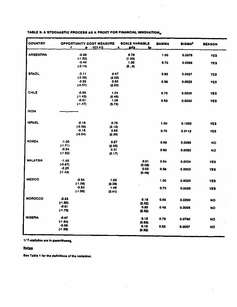
TABLE 3: A STOCHASTIC PROCESS AS A PROXY FOR FINANCIAL INNOVATIONO

COUNTRY OPPORTUNITY COST MEASURE SCALE VARIABLE GAMMA IOGMA SEASONI p II(14d) a gdo Ip

ARGENTINA -0.29 0.76 1.00 0.0078 YES(.1.52) (1.93).0.44 1.00 0.70 0.0062 YES

(.2.14) (2..9)

BRAZIL .3.11 0.47 0.63 0.0027 YES(.3.36) (2.02)-3.26 0.60 0.5 0.0025 YES

(-4.07) (2.60)

CHILE .0.50 1.04 0.75 0.0035 YES(.1.45) (5.46)*0.51 1.06 0.53 0.0033 YES

(.1.47) (5.79)

INDIA

ISRAEL .0.16 0.76 1.00 0.1255 YES(.0.58) (2.15)*0.15 0.89 0.70 0.0112 YES

(40.54) (2.36)

KOREA t1.00 0.27 0.86 0.0058 NO(.1.71) (2.05)*0.94 0.31 0.60 0.0053 NO

(.1.52) (2.17)

MALAYSIA *1.69 0.01 0.84 0.0004 YES(0.97) (0.09)-2.25 0.03 0.59 0.0003 YES

(.1.43) (0.49)

MEXICO -0.54 1.02 1.00 0.0025 YES(.09) (2.39)-0.83 1.46 0.70 0.0026 YES

(.1.56) (3.41)

MOROCCO 40.53 0.19 0.68 0.0200 NO(.1.90) (2.62)

0.51 0.20 0.48 0.0006 NO(.1.75) (2.52)

NIGEfRA .0.67 0.12 0.79 0.0790 NO(.1.84) (0.63).0.59 0.10 0.55 0.0057 NO

(.1.56) (0.55

1/T-stalIs are In poernthnset.

Be* Table I for he defin Wons of the varisble.

TABLE 4: MOST *PLAUSIBLE SPECIFICAllON

COUNTRY OPPORUJNITY COST SCALE VARIABLE liME METHOD OF ESTIMAllONI p 1/(1+n c gdp ip OLS TV1 BOTH NEITHER

ARGENTnNA X X X X

BRAZIL X X X X X

CHILE X X X

INDIA X X X

ISRAEL, X X X X

KOREAv X X X X

MALAYSIA X X X

MEXICO X X X

MOROCCO X X X

NIGERIA X X X

1/ If M2fMI Is used as a proxy for finaial lnnovaUon, coineon oban

Note

See Table for te defI of die variabls.WI: tunevarying frtee

TABLE 5: HOW MUCH OF THE EXPLAINED VARIATION IS ACCOUNTED BY FINANCIAL INNOVATION?(Shares)

COUNTRY GAMMA .-.- OLS WITH TREND -~ -TIME-VARYING INTERCEPT- AVERAGEOpportunity Scale Financial Opportunity Scale Financial INFLATION

Cost Variable Variable Innovation Cost Variable Variable Innovation(1) (2) (3) (4) (5) (6) (7) 8

ARGENTINA 1.00 0.06 0.34 0.59 0.06 0.30 0.64 261.1

BRAZIL 0.83 0.31 0.07 0.62 0.94 0.02 0.04 95.3

CHILE 0.75 0.26 0.60 0.14 0.06 0.76 0.18 49.8

INDIA - 0.01 0.65 0.14 -.------ *8.7

ISRAEL 1.00 0.29 0.10 0.61 0.01 0.37 0.61 106.2

KOREA 0.86 0.04 0.81 0.15 0.10 0.24 0.66 15.6

MALAYSIA 0.64 ---- 0.22 0.00 0.78 15.4

MEXICO 1.00 0.11 0.00 0.89 0.06 0.51 0.43 75.3

MOROCCO 0.68 0.33 0.64 0.03 0.11 0.14 0.75 8.2

NIGERIA 0.79 0.31 0.42 0.26 0.10 0.04 0.85 18.6

Figure 1: GAMMA

1.1 1_I

Mexico Israel Argentina1 1 ~~o oo

E 9 Korea

E I c Malaysia BrazilCD

0.8 o Nigeria

° Chile

0.7 _ Morocco

0.6 - -0 40 80 120 160 200 240 280

Average Inflation (yearly)

Figure 2: Share of Financial Innovation(time trend equations)

0.9 -'Mexico

0.8 -

0.7 -Brazil Argentina

0.6- ° Israel

0.5-

" 0.4-

0.3 - c) Nigeria

0.2- : Korea Chile

0.1- ° India

o Morocco0- I 1 , I , I

0 40 80 120 160 200 240 280Average Inflation

Figure 3: Share of Financial Innovation(time-varing intercept equations)

0.9a Nigeria

0.8- 0 Malaysia0.7 - Morocco Argentina

0.6 - °Korea O Israel

* 0.5-0 Mexico

'' 0.4-

0.3 -

0.2 - Chile

0.1 - Brazil0~~~~~~

0 40 80 120 160 200 240 280Average Inflation

PRE Working Paper Series

Contactliv Aufthor 1a for 1aper

WPS702 Should Price Reform Proceed Sweder van Wijnbergen June 1991 M. StroudeGradually or in a 'Big Bang?" 38831

WPS703 The Political Economy of Fiscal Sebastian Edwards June 1991 A. BhallaPolicy and Inflation in Developing Guido Tabellini 37699Countries: An Empirical Analysis

WPS704 Costs and Finance of Higher Rosemary Bellew June 1991 C. CristobalEducation in Pakistan Joseph DeStefano 33640

WPS705 What Causes Differences in Abby Rubin Riddell June 1991 C. CristobalAchievement in Zimbabwe's Levi Martin Nyagura 33640Secondary Schools?

WPS706 Successful Nutrition Programs in Eileen Kennedy June 1991 0. NadoraAfrica: What Makes Them Work? 31091

WPS707 Population, Health, and Nutrition: Population, Health, June 1991 0. NadoraFiscal 1990 Sector Review and Nutrition Division, 31091

Population and HumanResources Department

WPS708 Nongovernmental Organizations and Jocelyn DeJong June 1991 0. NadoraHealth Delivery in Sub-Saharan Africa 31091

WPS709 An Empirical Macroeconomic Model Luis Serven June 1991 S. Jonnakutyfor Policy Design: The Case of Chile Andres Solimano 39074

WPS710 Urban Property 1ax Reform: William Dillinger June 1991 V. DavidGuidelines and Recommendations 33734

WPS711 Financial Reform in Socialist Millard Long June 1991 M. RaggambiEconomies in Transition Silvia B. Sagari 37657

WPS712 Foreign Direct Investment in Thomas L. Brewer June 1991 S. King-WatsonDeveloping Countries: Patterns, 31047Policies, and Prospects

WPS713 The Determination of Wages in Simon Commander June 1991 0. Del CidSocialist Economies: Some Karsten Staehr 39050Microfoundations

WPS714 Wornen in Forestry in India Ravinder Kaur July 1991 A. Sloan35108

WPS715 Promoting Girl's and Women's Rosemary Bellew July 1991 C. CristobalEducation: Lessons from the Past Elizabeth M. King 33640

WPS716 Financing Training: Issues and Christopher Dougherty July 1991 C, CristobalOptions Jee-Peng Tan 33640

PRE Working Paper Series

Contact1 AuthoDr

WPS717 Does Financial Liberalization Really Jacques Morisset July 1991 S. King-WatsonImprove Private Investment in 31047Developing Countries?

WPS718 Impact of Investment Policies on Andrea Gubitz July 1991 S. King-WatsonGerman Direct Investment in Developing 31047Countries: An Empirical Investigation

WPS719 How Trade and Economic Policies Ramon Lopez July 1991 M. GunasekaraAffect Agriculture: A Framework for Ridwan Ali 32261Analysis Applied to Tanzania and Bjorn LarsenMalawi

WPS720 The Outlook for Commercial Bank Ellen Johnson Sirleaf July 1991 S. King-WatsonLending to Sub-Saharan Africa Francis Nyirjesy 31047

WPS721 The Demand for Money in Developing Patricio Arrau July 1991 S. King-WatsonCountries: Assessing the Role Jos6 De Gregorio 31047of Financial Innovation Carmen Reinhart

Peter Wickham