On Exports and Economic Growth

SWP508

World Bank Staff Working Paper No. 508

Februa 1962

'"-w? FUND

"H[ 2 1Q^22

jfjL " !.1 -U*{, D. C' -

_ tr5hxi FederDeve4lent Researh Cnter

N.W.

Wast*on D.C. 20433, USAU

Theewald5hd>l*oiFIgLE COPYThes v4ew. tvd kbwepr.Wlom in ft doarmwt arm ftho of the &Ahorsan shid iiot be sautzed to Xw V%AId Ba to b afilWido.prt~zMm, or to any hndM adbi k behff.

Pub

lic D

iscl

osur

e A

utho

rized

Pub

lic D

iscl

osur

e A

utho

rized

Pub

lic D

iscl

osur

e A

utho

rized

Pub

lic D

iscl

osur

e A

utho

rized

Pub

lic D

iscl

osur

e A

utho

rized

Pub

lic D

iscl

osur

e A

utho

rized

Pub

lic D

iscl

osur

e A

utho

rized

Pub

lic D

iscl

osur

e A

utho

rized

The views and interpretations in this document are those of the authors andshould not be attributed to the World Bank, to its affiliated organizationsor to any individual acting in their behalf.

WORLD BANK

Staff Working Paper No. 508

February 1982

ON EXPORTS AND ECONOMIC GROWTH

The paper analyses the sources of growth in the period 1964-1973 for agroup of semi-industrialized less developed countries. An analyticalframework is developed, incorporating the possibility that marginal factorproductivities are not equal in the export and non-export sectors of theeconomy. Econometric analysis utilizing this framework indicates thatmarginal factor productivities are significantly higher in the exportsector. The difference seems to derive, in part, from inter-sectoralbeneficial externalities generated by the export sector. The conclusionis therefore that growth can be generated not only by increases in theaggregate levels of labor and capital, but also by the reallocation ofexisting resources from the less efficient non-export sector to the higherproductivity export sector.

Prepared by:Gershon Feder, Development Research Center

Copyright ( 1982The World Bank1818 H Street, N.W.Washington, D.C. 20433U.S.A.

ON EXPORTS AND ECONOMIC GROWTH

I. Introduction

The relation between export performance and economic growth has

been a subject of considerable interest to development economists in

recent years. Empirical observations across countries tended to demonstrate

that developing countries with a favorable export growth record tended

to enjoy higher rates of growth of national income. Obviously, since

exports are a component of aggregate output, one would expect a positive

association in terms of the correlation coefficient [Kravis (1970)]. But

several empirical studies argued that exports contribute to GDP growth more

than just the change in the volume of exports [Balassa (1978), Heller and

Porter (1978), Michaely (1977), Michalopoulos and Jay (1973)].

Explanations for these observations were discussed by a number

V of economists, highlighting various beneficial aspects of exports, such as

greater capacity utilization, economies of scale, incentives for techno-

logical improvements and efficient management due to competitive pressures

abroad [see Balassa (1978), Keesing (1967, 1969), Krueger (1980), and

Bhagwati and Srinivasan (1978)]. The implication of these discussions is

that there are substantial differences between marginal factor productivities

in export-oriented and non-export-oriented industries, such that the former

have higher factor productivity. It follows, then, that countries which

have adopted policies less biased against exports benefitted from closer-

to-optimal resource allocation and higher growth.

The present paper develops an analytical framework for the

quantitative assessment of factor productivity differentials between

exports and non-exports using aggregate data. This framework is utilized

-2-

in an empirical study of sources of growth in a sample of semi-industrialized

less developed countries within the decade 1964-1973. The analysis allows

an estimate of the sectoral marginal productivities. Furthermore, the

extent of inter-sectoral beneficial externalities generated by exports can

be specifically identified. The results highlight the role of export

performance in explaining the growth record of the sample countries.

II Framework of Analysis

The analysis in this paper adopts a supply side description of

changes in aggregate output. In so doing, it follows a practice widely

used in the empirical study of sources of growth [see, e.g., Hagen and

Hawrylyshyn (1969) and Robinson (1971)]. Within such a framework, where

aggregate growth is related to changes in capital and labor through an

underlying production function, the studies of Balassa (1978), Chenery

et al (1970), and Michalopoulos and Jay (1973) have included an indicator

of export performance among the variables explaining growth.-/ In the

following, a framework is developed which provides a formal rationalization

for the incorporation of export variables in the sources of growth equation.

Furthermore, starting from the sectoral production functions, a proper

specification of export variables is indicated and a non-conventional inter-

pretation of parameters is implied.

Since the present analysis focuses on the potential non-optimality

of resource allocation between export and non-export sectors, the economy

is viewed as if it consists of two distinct sectors: one producing export

1/ Chenery et al represent exports performance by export growth multipliedby export share; the other works include exports growth.

-3-

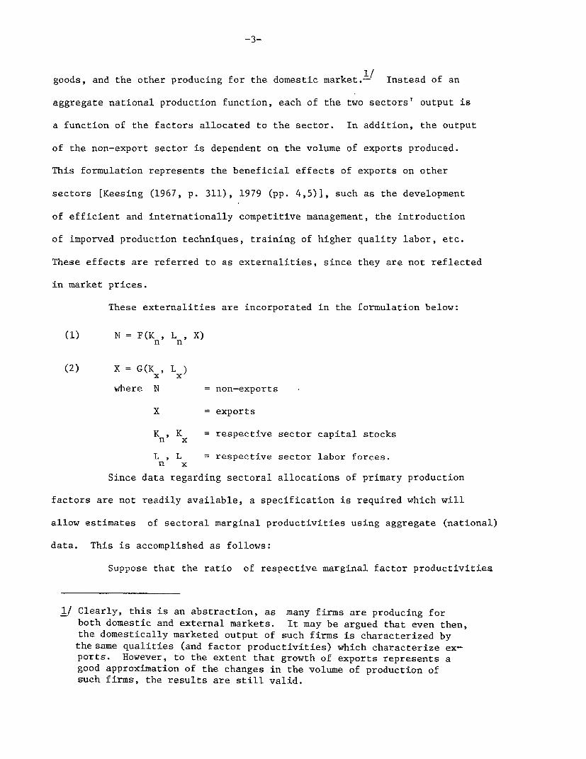
goods, and the other producing for the domestic market.-/ Instead of an

aggregate national production function, each of the two sectors' output is

a function of the factors allocated to the sector. In addition, the output

of the non-export sector is dependent on the volume of exports produced.

This formulation represents the beneficial effects of exports on other

sectors [Keesing (1967, p. 311), 1979 (pp. 4,5)], such as the development

of efficient and internationally competitive management, the introduction

of imporved production techniques, training of higher quality labor, etc.

These effects are referred to as externalities, since they are not reflected

in market prices.

These externalities are incorporated in the formulation below:

(1) N = F(K , Ln, X)

(2) X = G(K , Lx)

where N = non-exports

X = exports

Kn, Kx = respective sector capital stocks

L , L = respective sector labor forces.n x

Since data regarding sectoral allocations of primary production

factors are not readily available, a specification is required which will

allow estimates of sectoral marginal productivities using aggregate (national)

data. This is accomplished as follows:

Suppose that the ratio of respective marginal factor productivities

1/ Clearly, this is an abstraction, as many firms are producing for

both domestic and external markets. It may be argued that even then,

the domestically marketed output of such firms is characterized by

the same qualities (and factor productivities) which characterize ex-

ports. However, to the extent that growth of exports represents a

good approximation of the changes in the volume of production of

such firms, the results are still valid.

-4-

in the two sectors deviates from unity by a factor 6 s i.e.,

(3) (Gk/Fk) (GL/FL) 1 + 6

where the subscripts denote partial derivatives.

Under certain ideal conditions (competition9 profit motivated

entrepreneurs 9 absence of various regulations and constraints, perfect

information, perfect mobility of factors), market forces would lead to a

situtation such that 6 = 0. In the absence of externalities, and for a

given set of prices, this situation would reflect an allocation of resources

which maximizes national output. However, the ideal conditions mentioned

above are not likely to obtain in most LDCs. Rather, due to a number of

reasons, marginal factor productivities are likely to be lower in the non-

export sector (i.e., 6 > 0). One important reason is the more competitive

environment in which export-oriented firms operate. Competition induces in-

novativeness, adaptability, efficient management of firms' resources, etc.

Another reason for deviations between sectoral marginal factor productivities

are various regulations and constraints such as credit and foreign exchange

rationing [Balassa, 1977]. The higher perceived uncertainty associated with

export enterprises may be another factor contributing to deviations in marginal

productivity. Productivity differentials which are due to externalities

are not included in 6 , as they will be specifically identified.

A differentiation of equations (1) and (2) yields

(4) N = Fk *I F L + F *X

(5) X = G I +G Lx

where In and I are respective sectoral gross investments, Ln and

-5-

L are sectoral changes in labor force, and F describes the marginal

externality effect of exports on the output of non-exports.

Denoting Gross Domestic Product by Y , and since by definition

Y = N+X , it follows

(6) Y = N + X

Using equations (3)-(5) in equation (6) yields

(7) Y Fk* In+ FL * Ln + Fx *X + (1 + 6) Fk Ix+( ) FL L

k n x L nx x k x L x-Fk* (In+ I )+FL (Ln + L + F *X +6 (Fk Ix +FL *L )

Define total investment I(=- I n I ) and total growth of labor

L (E L +L ). Recall that equations (3) and (5) imply

n x~~~~~~

(8) F ' I + F '~~~ L x 1+ (G I +G *L ) = (8) F *k I +F *L = +6 k x L x 1+6

Using this result in equation (7) finally yields

(9) Y Fk I + FL L + ( 1+6 x

Following arguments similar to those presented by Bruno (1968),

suppose that a linear relationship exists between the real marginal

productivity of labor in a given sector and average output per laborer

in the economy, say

(10) FL = * (Y/L)-

Then, dividing equation (9) through by Y and denoting Fk i a

yields, after some manipulation

(11) y I+ L + F X . X= +y jjL 1 +6 +x] x y

-6-

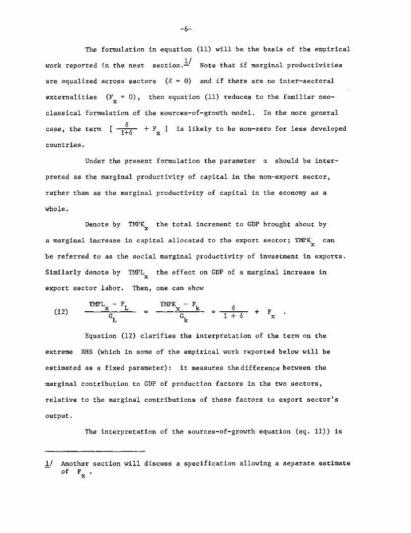
The formulation in equation (11) will be the basis of the empirical

work reported in the next section.-/ Note that if marginal productivities

are equalized across sectors (6 = 0) and if there are no inter-sectoral

externalities (F = 0), then equation (11) reduces to the familiar neo-

classical formulation of the sources-of-growth model. In the more general

case, the term 6 + F ] is likely to be non-zero for less developed1+6 x

countries.

Under the present formulation the parameter a should be inter-

preted as the marginal productivity of capital in the non-export sector,

rather than as the marginal productivity of capital in the economy as a

whole.

Denote by TMPKx the total increment to GDP brought about by

a marginal increase in capital allocated to the export sector; TMPK can

be referred to as the social marginal productivity of investment in exports.

Similarly denote by TMPLx the effect on GDP of a marginal increase in

export sector labor. Then, one can show

TMPLx FL TNPK -Fk 6(12) = _ + FGL Gk 1+ 6 x

Equation (12) clarifies the interpretation of the term on the

extreme RHS (which in some of the empirical work reported below will be

estimated as a fixed parameter): it measures the difference between the

marginal contribution to GDP of production factors in the two sectors,

relative to the marginal contributions of these factors to export sector's

output.

The interpretation of the sources-of-growth equation (eq. 11)) is

1/ Another section will discuss a specification allowing a separate estimateof F

x

-7-

then straightforward: the rate of growth of GDP is composed of the

contribution of factor accumulation (i.e., growth of capital and labor)

and the gains brought about by shifting factors from a low productivity

sector (non-exports) to a high real productivity sector (exports).

II B. Econometric Formulation

Equation (11) was used for a cross-country regression relating the

rate of growth of GDP (in constant prices) to the share of investment in

GDP, growth of labor (proxi for labor growth) and to the growth of exports

(in constant prices) multiplied by exports share in GDP.

The study focuses on a group of less developed countries defined by

Chenery (1980) as semi-industrialized. The definition involves both relative

and absolute indicators (such as the share of industrial output in GNP

and the level of per capita industrial output). Since the indicators do

not necessarily overlap, Chenery (1980) distinguishes between those countries

which are only "marginally" semi-industrialized, and those which qualify

under a stricter definition. Accordingly, the study provides estimates

for the sample defined by the strict definition (19 countries) as well as

a larger sample (31 observations) including also marginal cases.

An issue which needs to be addressed is the length of time to

be covered by any single country observation. Earlier studies used 5-10

year averages, since annual data include substantial random effects which

tend to be eliminated by the procedure of averaging. The existence of

lagged responses is another element which becomes less severe when averages

rather than annual data are used. This study uses averages defined over the

decade 1964-1973.

-8-

There are a host of econometric problems related to cross-

country aggregate analysis of growth (e.g., possibility of simultaneous

determination of both dependent and explanatory variables). Some of

these complications are discussed by Hagen and Hawrylyshyn (1969) and by

Chenery et al (1970), and will not be repeated here. The constancy

of parameters across observations merits, however, some further elabor-

ation. Any cross-country study assumes implicitly that parameters

are in some general way similar across countries. In a production

function context, different countries are thus assumed to operate with

identical production functions. In studies where the production function

framework is complicated further by the existence of non-optimal allo-

cation, an additional assumption is involved, namely, that the degree of

misallocation (as indicated by the RHS of equation (12)) is similar across

countries.

These problems need to be borne in mind when parameters are

interpreted. It is probably better to treat the estimated coefficients

as average values which provide a general order of magnitude within the

sample but are not applicable to any specific country. An attempt will

be made in a latter section to allow for a possibility of variation

across observations in the externality effect Fx . We set out now,

however, to estimate equation (11) in the form

(13) Y a.I + L+ y XY Y L prti)

where the parameter y represents the differential productivities of

-9-

factors, as explained earlier. It is expected that a , the marginal

productivity of capital in the non-export sector, will be positive but

it's magnitude should be less than the figures in the range 0.2-0.35

which were reported by earlier studies-/ based on an aggregate

macro production function. The reason is that in such studies the estimated

parameter is some average (although not necessarily properly weighted) of

marginal productivities in the two sectors, and is thus likely to be higher

than a specific estimate of marginal productivity in the low productivity

sector. The hypothesis that marginal productivities in the export sector

are higher and that exports generate beneficial externalities suggests

that the parameter y should be positive and significantly different from

zero. The parameter 5 , related to labor growth, should also be signifi-

cantly more than zero if labor surplus was not the prevalent situation in

sample countries during the period covered.

III. Empirical Analysis

III.A. Empirical Results of the Basic Formulation

Table 1 reports the results of two specifications of the re-

gression equation: One, referred to as the conventional neoclassical

model,assumes that y = 0 , and thus presents GDP growth as the result

of capital and labor growth only. The second specification follows

equation (13). Comparison of the two specifications highlights,

therefore, the superior explanatory power of equation (13). For both

samples, the adjusted R is almost doubled when the specification

1/ For example, Humphries (1976) reports figures in the range 0.25-0.33;Pesmazoglu (1972) reports estimates in the range 0.17-0.35.

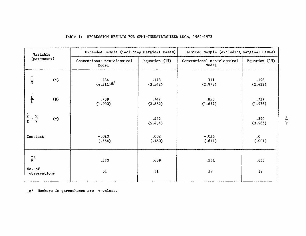
Table 1: REGRESSION RESULTS FOR SEMI-INDUSTRIALIZED LDCs, 1964-1973

Variable Extended Sample (including Marginal Cases) LImited Sample (excluding Marginal Cases)_]

(parameter) Conventional neo-classical Equation (15) Conventional neo-classical Equation (15)

Model Model

I~~~~~~~~~~~~~~~~~~~~~~~~~~~~~~~~~~~~~~~~~~~~~~~~~~~~~~~~~~~~~~~~~~~~~~~~~~~~~~~~~~~~~~

I (a) e284 .178 .311 .196

(4.311)a/ (3.542) (2.973) (2.432)

L .739 .747 .853 .737

L (1.990) (2.862) (1.652) (1.976)

x x .(Y) 0422 .390

(5.454) (3.985)

Constant -.010 .002 -.016 .0

(.554) (.180) (.611) (.001)

F2R2 .370 .689 .331 .653

No. of 31 31 19 19

observations

a/ Numbers in parentheses are t-values.

-11-

allowing for differences in marginal productivities is used. The

results lend strong support to the hypothesis that marginal factor

productivities in the export sector are higher than in the non-export

sector, as the coefficient of X -Xy is positive and significantly

different from zero. The sign and magnitude of the coefficient related

to investment are within the range expected. Specifically, when the

conventional neo-classical formulation is used, the estimated parameter

is within the range observed in earlier studies. When the formulation

of equation (13) is adopted, the parameter declines sharply.

The parameter associated with labor growth (which, as explained

earlier, reflects the relation between marginal labor productivity and

average output per laborer) is significantly greater than zero.-/ This

may be taken as an indication that surplus labor was not the general case for

sample countries in the period under investigation.

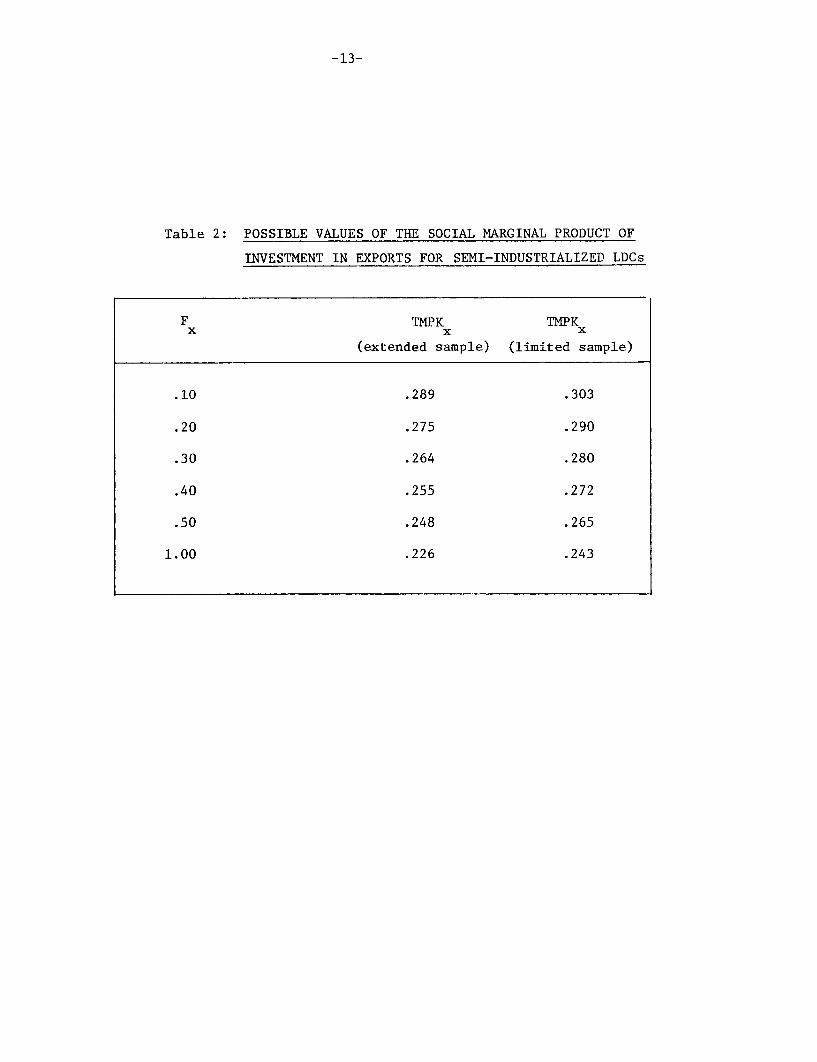
The point estimate for y can be used further to provide some

information on the social marginal productivity of capital in export

(TMPK ). Recalling equation (12), it is noted that TMPK = (1 + F)* Gk

thus

(14) TMPK = Fk ' (1 + F )/(l - y + FX)

While Fk and y were estimated, F is not known (in a later section

of this chapter some direct estimates of Fx will be obtained). For a

plausible range of Fx values one can, however, calculate the corresponding

values of the social marginal product of investment in exports, using equation (14).

1/ With a 5% one-tailed test.

-12-

These are presented in Table 2.

It should be emphasized that the estimates reported in Table 2

are strictly consistent for only one particular (and unknown) value of

F . This follows from the fact that y incorporates Fx , and thus

varying the latter while holding y fixed is not strictly legitimate.

However, it is evident from these calculations that the marginal value

to the economy from a unit investment in exports expansion is substantially

higher than that of investment in non-exports. While these numbers

correspond to sample averages, they provide strong support to the view

that the success story of export-led economies such as Korea

is due in large part to the enormous shift of resources into the higher

productivity export sector.

III B. Specifying the Externality Effect and Empirical Results

So far we were not able to decompose the factor productivity

differential y into its components. One can identify the specific inter-

sectoral externality effect by adopting a plausible specification for the

term Fx . Suppose that exports affect the production of non-exports

with constant elasticity, i.e.,

(15) N = F(Kn Ln X) = X e (K , L )

where e is a parameter. One can show

(16) aN F x0-DX x X

Equation (11) can now be rewritten

(17) y= I * c + N X X

But N a N/Y = . [l-(X/Y)l = 0=0 /Y(XIY) (X/Y)

-13-

Table 2: POSSIBLE VALUES OF THE SOCIAL MARGINAL PRODUCT OF

INVESTMENT IN EXPORTS FOR SEMI-INDUSTRIALIZED LDCs

F TMPK TMPKx x x

(extended sample) (limited sample)

.10 .289 .303

.20 .275 .290

.30 .264 .280

.40 .255 .272

.50 .248 .265

1.00 .226 .243

-14-

ITsing this result, equation (17) is rearranged, obtaining

(18 I L (SX x x(18) Y = a y + ff °- +( - -e) X ° Y + 0 °

Note that if it is assumed 0 = e 9 the model reduces to

y I + a L + XY Y L X

which is essentially the equation adopted by Michaelopoulos and Jay (1973)

and Balassa (1977).-/

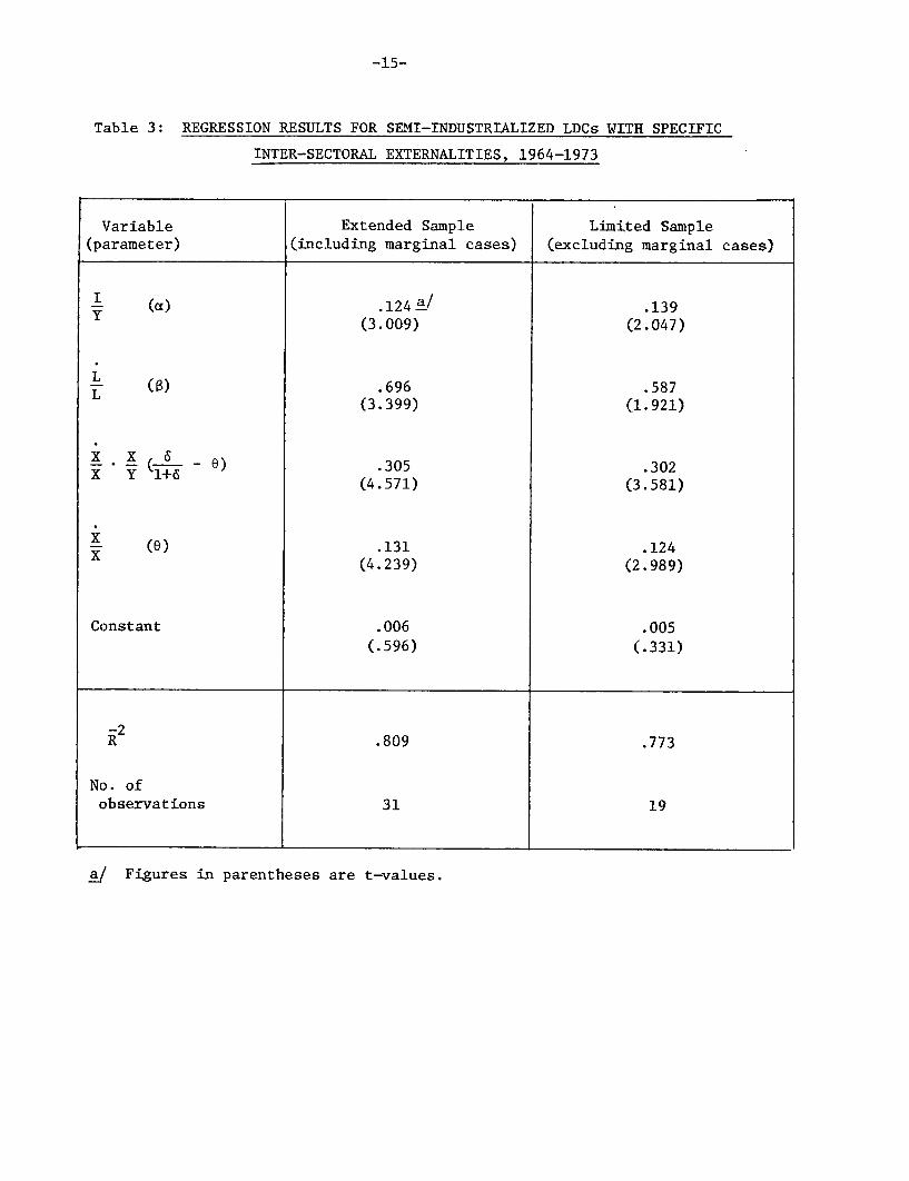
Results of regressions adopting the specification of equation (18)

are reported in Table 3.

The modified formulation increases the explanatory power of the

model considerably. The results indicate that the inter-sector externality

parameter (0) is statistically significant in both samples. The mag-

nitude of the estimated parameter is quite substantial. If exports are

increased by 10% without withdrawing resources from the non-export-sector,

the latter grows by approximately 1.3%. The other component of productivity

differential (the parameter 6 ) can be calculated given the estimate of 0

and the parameter associated with X ° X . The result is 6 - .75

implying that there is a substantial productivity differential between exports

and non-exports in addition to the differential due to externalities.

The coefficients of investment share and labor growth are

within the same order of magnitude of the estimates obtained in Table 2,

and are statistically significant.-/

1/ These works make a distinction between domestic capital and foreigncapital flows. Such a distinction was experimented with in variousregressions under the present study, but no (statistically) significantdifference was indicated.

2/ At a 5% one-tailed test.

-15-

Table 3: REGRESSION RESULTS FOR SEMI-INDUSTRIALIZED LDCs WITH SPECIFIC

INTER-SECTORAL EXTERNALITIES, 1964-1973

Variable Extended Sample Limited Sample(parameter) (including marginal cases) (excluding marginal cases)

I (a) .124 a/ .139(3.009) (2.047)

L (U) .696 .587(3.399) (1.921)

_- _Y &d 0+ ) .305 .302X Y l+~~~~~S (4.571) (3.581)

X (0) .131 .124X (4.239) (2.989)

Constant .006 .005(.596) (.331)

-2R .809 .773

No. ofobservations 31 19

a/ Figures in parentheses are t-values.

-16-

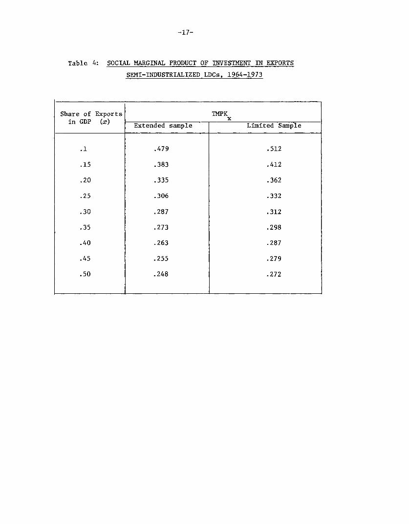
Using the results of Table 3, the social marginal product of

investment in exports (TMPK ) can be calculated. Recall from equation

(16) Fx = e x , where x is the share of exports in GDP. It

follows then,

y(x) = +6 + e ° and equation (14) can be written

(19) TMPK =F (1 + e l )° (1 +6)x k

Using the parameters reported in Table 3, equation (19) generates

the social marginal product of investment in exports for economies with

different values of x v These are presented in Table 4.

The calculations in Table 4 are free of the inconsistencies as-

sociated with the numbers presented in Table 2. Again, it is demonstrated

that, at the margin, investment in the export sector has a substantially

higher social marginal productivity than investment in non-exports. The

differential is smaller in economies where a large share of resources is

already allocated to the export sector, as in such economies the inter-sector

externality effect is smaller.

III C. Sources of Growth

Using the results of Table 3 and the mean values of sample variables,

the average rate of GDP growth in the period 1964-1973 can be decomposed

so as to identify the contributions of aggregate investment, labor force

growth and resource shifts into exports. This is done in Table 5 for both

samples. The results indicate that the gain in productivity due to closer-

to-optimal allocation associated with export expansion contributed more

than 2.2 percentage points to the growth of the strictly semi-industrialized

countries, and close to 108 percentage points if the less strict definition

-17-

Table 4: SOCIAL MARGINAL PRODUCT OF INVESTMENT IN EXPORTS

SEMI-INDUSTRIALIZED LDCs, 1964-1973

Share of Exports TMPKin GDP (x) _ xExtended sample Limited Sample

.1 .479 .512

.15 .383 .412

.20 .335 .362

.25 .306 .332

.30 .287 .312

.35 .273 .298

.40 .263 .287

.45 .255 .279

.50 .248 .272

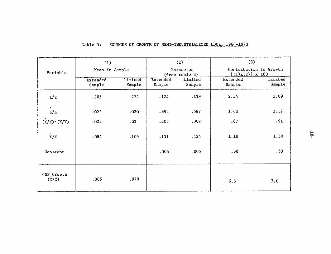
Table 5: SOURCES OF GROWTH OF SEMI-INDUSTRIALIZED LDCs, 1964-1973

(1) (2) (3)

Variable Mean in Sample Parameter Contribution to Growtha__________________________ (from table 3) [(l)x(2)] x 100

Extended Limited Extended Limited Extended LimitedSample Sample Sample Sample Sample Sample

I/Y .205 .222 .124 .139 2.54 3.09

L/L .023 .020 .696 .587 1.60 l117

(X/X) (X/Y) .022 .03 .305 .302 .67 .91

XI/X .084 .105 .131 .124 1.10 1.30

Constant .006 .005 .60 .53

GDP Growth(Y/Y) .065 .070 6.5 7.0

-19-

of industrialization is used. The contribution of exports can be decom-

posed into two components: (i) The gain due to beneficial externalities

affecting the non-export sector (which equals e.(l-x).(X/X)); (ii) The

gain due other elements underlying higher factor productivity in the

export sector ((T-S) *X * y)

The calculations for the extended sample reveal that .81 of one

percentage point is due to inter-sectoral externalities, and .96 is due

to other effects. The corresponding figures for the limited sample are

.93 and 1.27. Thus, slightly less than half of the gain in growth due

to higher factor productivity in exports is due to inter-sectoral

externalities.

IV Concluding Remarks

This paper provides evidence supporting the view that the

success of economies which adopt export-oriented policies is due, at

least partially, to the fact that such policies bring the economy closer

to an optimal allocation of resources. The estimates show that there are,

on average, substantial differences in marginal factor productivities

between the export and non-export sectors. These differences derive in part

from the failure of entrepreneurs to equate marginal factor productivities

and in part due to externalities. The latter are generated because the

export sector confers positive effects on the productivity in the other

sector, but these are not reflected in market prices.

The results are such that social marginal productivities are higher

in the export-sector, and economies which shift resources into exports will

gain more than inward-oriented economies. The empirical findings suggest

-20-

that even when entrepreneurs optimize resource allocation given the prices

they face, there are substantial gains to be made due to the externality

effects.

Most of the countries covered by this sample have a relatively

high component of industrial goods in their exports, compared to the

average for less developed countries. This may be taken as an indication,

but not yet as solid evidence, to.support the view that externality effects

are generated largely by industrial exports.

The analytical framework developed in this study can be utilized

in studies using more detailed data such that the extent of productivity

differentials in specific groups of countries (with different policy

orientation) can be assessed. Similarly, the relation between inter-

sector externalities and export composition can be clarified further

using the same analytical framework.

-21-

APPENDIX

SOURCES OF DATA AND DEFINITIONS

1. Calculation of variables

All data were obtained from World Tables 1980. Variables were

calculated from time series for the period 1964-1973 in constant prices.

Average rates of growth were obtained by regressing kn Zt = a + b-t

where Zt is the economic variable under consideration and t is time.

The rate of growth, say r , is then calculated as r = e b- 1 . Average

ratios (Investment/GDP , Export/GDP) were calculated as simple averages

for the decade.

Table A.1 presents means and standard deviations of the variables

used in the study.

Table Al: Characteristics of the Samples of Semi-

Industrialized LDCs 1964-1973

Mean(Standard Devi ation)

Variable Extended LimitedSample Sample

GDP Growth .065 .070(.022) (.025)

Investment/GDP .205 .222(.050) (.047)

Population Growth .023 .020(.009) (.009)

Exports Growth .084 .105(.070) (.080)

Export Share .235 .266(.225) (.282)

(Export Growth) x .022 .030Export Share (.032) (.038)

-22-

2. Composition of Samples

Following Chenery (1980), the strict definition of semi-

industrialized LDCs applies to the following economies which are

included in the "limited sample": Argentina, Brazil, Chile, Taiwan (China),

Colombia, Costa Rica, Greece, Hong-Kong, Israel, Korea, Malaysia,

Mexico, Portugal, Singapore, South Africa, Spain, Turkey, Uruguay and

Yugoslavia. In addition, Ireland and Venezuela fall under the strict

definition but were excluded from the sample; the former is defined

by the World Bank as a developed country and the latter is a major

oil exporter. Countries which are considered as marginally semi-

industrialized were added to the limited sample creating the "extended

sample." These countries are: Dominican Republic, Ecuador, Egypt,

Guatemala, India, Ivory Coast, Kenya, Morocco, Peru, Philippines,

Syria, Thailand and Tunisia. In addition, Iran, Iraq and Algeria are

defined as marginal cases but were excluded from the sample, being major

oil exporters.

-23-

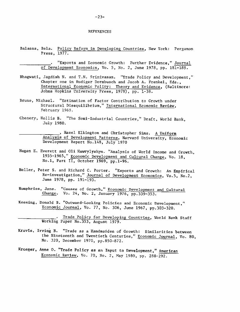
REFERENCES

Balassa, Bela. Policy Reform in Developing Countries, New York: PergamonPress, 1977.

. "Exports and Economic Growth: Further Evidence," Journalof Development Economics, Vo. 5, No. 2, June 1978, pp. 181-189.

Bhagwati, Jagdish N. and T.N. Srinivasan. "Trade Policy and Development,"Chapter one in Rudiger Dornbusch and Jacob A. Frenkel, Eds.,International Economic Polity: Theory and Evidence, (Baltimore:Johns Hopkins University Press, 1978), pp. 1-38.

Bruno, Michael. "Estimation of Factor Contribution to Growth underStructural Disequilibrium," International Economic Review,February 1968.

Chenery, Hollis B. "The Semi-Industrial Countries," Draft, World Bank,July 1980.

, Hazel Elkington and Christopher Sims. A UniformAnalysis of Development Patterns, Harvard University, EconomicDevelopment Report No.148, July 1970

Hagen E. Everett and Oli Hawrylyshyn. "Analysis of World Income and Growth,1955-1965," Economic Development and Cultural Change, Vo. 18,No.1, Part II, October 1969, pp.1-9 6.

Heller, Peter S. and Richard C. Porter. "Exports and Growth: An EmpiricalRe-investigation," Journal of Development Economics, Vo.5, No.2,June 1978, pp. 191-193.

Humphries, Jane. "Causes of Growth," Economic Development and CulturalChange. Vo. 24, No. 2, January 1976, pp.339-353.

Keesing, Donald B. "Outward-Looking Policies and Economic Development,"Economic Journal, Vo. 77, No. 306, June 1967, pp.303-320.

. Trade Policy for Developing Countries, World Bank StaffWorking Paper No.353, August 1979.

Kravis, Irving B. "Trade as a Handmaiden of Growth: Similarities betweenthe Nineteenth and Twentieth Centuries," Economic Journal, Vo. 80,No. 320, December 1970, pp.850-872.

Krueger, Anne 0. "Trade Policy as an Input to Development," AmericanEconomic Review, Vo. 70, No. 2, May 1980, pp. 288-292.

-24-

Michaely, Michael. "Exports and Growth: An Empirical Investigation,"Journal of Development Economics, Vo. 4, No. 1, March 1977, pp.49-53.

Michalopoulos, Constantine and Keith Jay. Growth of Exports and Income inthe Developing World: A Neoclassical View, A,I.D. DiscussionPaper No.28, Washington, D.C., NOvember 1973.

Pesmazoglu, John. Growth, Investment and Saving Ratios: Some Long andMedium Term Associations by Groups of Countries," Bulletin ofOxford University Institute of Economics and Statistics, Vo.34,No. 4, November 1972, pp. 30 9 - 32 8 .

Robinson, Sherman. "Sources of Growth in Less Developed Countries,"Quarterly Journal of Economics, Vo. 85, No. 3, August 1971,pp .391-408.

World Bank, World Tables, Washington, D.C., 1980.