Public Disclosure Authorized Christopher J. A ...
27
World Bank Reprint Series: Number 382 Christopher J. Heady and Pradeep K. Mitra A Computational Approach to Public Policies Reprinted with pennission from Mathenmatical Programming Study, vol. 23, (1985), pp. 95-120, published by North Holland, Amsterdam. Public Disclosure Authorized Public Disclosure Authorized Public Disclosure Authorized Public Disclosure Authorized Public Disclosure Authorized Public Disclosure Authorized Public Disclosure Authorized Public Disclosure Authorized
Transcript of Public Disclosure Authorized Christopher J. A ...

World Bank Reprint Series: Number 382
Christopher J. Heady and Pradeep K. Mitra
A Computational Approach toPublic Policies
Reprinted with pennission from Mathenmatical Programming Study, vol. 23, (1985), pp. 95-120,published by North Holland, Amsterdam.
Pub
lic D
iscl
osur
e A
utho
rized
Pub
lic D
iscl
osur
e A
utho
rized
Pub
lic D
iscl
osur
e A
utho
rized
Pub
lic D
iscl
osur
e A
utho
rized
Pub
lic D
iscl
osur
e A
utho
rized
Pub
lic D
iscl
osur
e A
utho
rized
Pub
lic D
iscl
osur
e A
utho
rized
Pub
lic D
iscl
osur
e A
utho
rized
Matlhematical Programming Study 23 (1985) 95-120North-Holland
A COMPUTATIONAL APPROACH TO OPTIMUMPUBLIC POLICIES
Christopher J. HEADYUniversity College London, Gower Street, WClE 6BT, UK
Pradeep K. MITRAThe World Bank, 1818 H Street, NW, Washington, DC 20433, USA
Received 25 June 1984Revised manuscript received 6 December 1984
This paper describes and illustrates the use of an algorithm that computes optimal taxes andpublic production in an economy where the government's tax powers are restricted. The specialfeatures of the optimal restricted tax problem required the solution of problems that have notarisen in previous applications of Scarfs algorithm. Indeed, these problems could only be dealtwith properly by developing two versions of the algorithm that can be used together.
This paper outlines the economic model and explains its special features. The two versions ofthe algorithm are then described and their convergence properties established. The combined useof the two versions of the algorithm is illustrated in a problem that involves the choice betweenpublic and private control of production and shows that domestic tax restrictions can makeinefficient public production desirable.
Key words: Optimal Taxation, Tax Restrictions, Public Production, Scarfs Algorithm.
1. Introduction
The problem
The fundamental theorem of welfare economics states that, under certain condi-tions, the maximum of a social welfare function which respects individual preferen-ces can be decentralized as a competitive equilibrium provided that the governmentcan redistribute endowments among individuals through a (nondistortionary) systemof lump-sum taxes and subsidies. (cf. Arrow and Hahn (1971)) The resulting prices,
Revised draft of an invited paper presented to a workshop on Tlhe Solution and Applicatiotn of EconomicEquilibrium Models held at Stanford University in June 1984. The work reported here was done whileHeady was visiting Queen's University at Kingston. The World Bank does not accept responsibility forthe views expressed herein which are those of the author(s) and should not be attributed to the WorldBank or to its affiliated organizations. The findings, interpretations, and conclusions are the results ofresearch supported by the Bank; they do not necessarily represent official policy of the Bank. T'hedesignations employed, the presentation of material, and any maps used in this document are solely forthe convenience of the reader and do not imply the expression of any opinion whatsoever on the partof the World Bank or its affiliates concerning the legal status of any country, territory, city, area, or ofits authorities, or concerning the delimitation of its boundaries, or national affiliation.
95
96 C.J. Heady, P.K. Mitra / A computational approach to optimum public policies
which are common to both consumers and producers, reflect social opportunitycosts while the lump sum transfers equate the margiinal social worth of the individualsin the economy. The so-called modern approach to public policy has (1) shownthat no agent in the eco.iomy will in general have any incentive to reveal to thegovernment information about his personal characteristics necessary to implementlump sum policies (Mirrlees (1981)) and (2) enquired what can be achieved whenthe only redistributive mechanisms potentially available to the government are(distortionary) taxes and subsidies on all goods and services. The most importantresult that can be established (Diamond and Mirrlees (1971)) states that themaximum of an individual preference-respecting social welfare function can bedecentralized via two sets of prices-consumer and producer prices with respect towhich consumers and producers respectively behave in a competitive way. Therelationship of those two prices with social opportunity costs (or 'shadow prices')is as follows. Producer prices equal shadow prices. The deviation of each consumerprice from the corresponding shadow price (or, equivalently, producer price) bal-ances two sets of considerations: (i) the efficiency loss arising from the distortionarytax and (ii) equity considerations as captured by the relative importance of thecommodity in the budgets of households in different circumstances (Atkinson andStiglitz (1980)). This result shows that the ability to tax all goods removes anyargument for interfering with the aggregate efficiency of production. Producer andshadow prices which guide private and public production decisions respectix ely arethe same so that there is no need to distinguish between the private and publicproduction sectors. All taxes act by driving a wedge between consumer prices andshadow prices, with the size of the wedge embodying the tradeoff, mentioned above,between efficiency and equity considerations. This is consistent with a generallyheld presumption (c.f. Bhagwati (1971)) that corrective policies (in this case, con-sumer taxation) should be targeted close to the area where the original 'distortion'was to be found, viz., the infeasibility of lump sum transfers capable of discriminatingamong consumers on the basis of their characteristics.
These results have led to an applicable set of prescriptions for cost benefit analysisin developing countries (Little and Mirrlees (1974)) and for tax-price reform (Drezeand Stern (1985)). However, some of these maxims depend critically on the assump-tion that it is possible to tax and subsidize all commodities in the economy, i.e., toinsert wedges between producer prices and consumer prices.' Casual empiricismsuggests, however, that the assumption, though fruitful for the development of thetheory, is unrealistic for most countries. Few countries have more than three differentrates of sales tax and we know of none that taxes different types of labour income(for example, skilled as compared to unskilled) at different rates. Furthermore,developing countries frequently find it impossible to tax transactions betweenagricultural producers and agricultural consumers in commodities such as food,
' The recommendation to evaluate a small country's tradeables at world prices for cost-benefit analysisdoes not depend on that assumption. (cf. Diamond and Mirrlees (1976)).

C.J. Heady, P.K. Mitra / A computational approach to optimum public policies 97
rural labour and land. Instead, taxes and subsidies are typically levied on theagricultural sector's net transactions with the rest of the economy and the outsideworld.
The introduction of tax restrictions implies that production efficiency ceases tobe desirable. This is because changes in the producer prices of goods subject to atax restriction will produce changes in their consumer prices. Thus, producer priceshave a role in determining consumer choice and utility, as well as in organizingproduction; in general, producer prices no longer equal shadow prices. (Stiglitz andDasgupta (1971)). This confers two potential social advantages on public production.The first, and more straightforward, is its ability to undertake activities that are notprofitable at private producer prices but profitable at shadow prices. The secondadvantage arises because the sole production of a good in the public sector, whenappropriate, no longer constrains private producer prices to satisfy zero privateprofitability in those activities (though positive profitability is of course ruled out).This degree of freedom can weaken the force of the tax restrictions (which linkproducer and consumer prices) by allowing the greater resulting variation in producerprices to be exploited with a view to obtaining better consumer prices.
Summary qf the paper
The restricted tax problem has a number of new features, both analytical andcomputational. It is necessary to keep track of three separate sets of prices: consumerprices, producer prices and shadow prices, as well as to distinguish clearly betweenprivate and public production possibilities. It also requires substantial modificationsto Scarf-type algorithms as applied to nonlinear programming probleni-s (Scarf(1973)) and extended by the authors to compute unrestricted optimal commoditytaxes (Heady and Mitra (1980)). The analytical aspects of the problem have beenexplored elsewhere, (Heady and Mitra (1982)), but, to make this presentationself-contained, are briefly repeated in Section 2. This paper concentrates primarilyon the computational issues and develops two algorithms which can be used tolocate restricted tax optima.
The computational difficulties will become clear in Section 3. However, to brieflyanticipate that discussion here, those difficulties derive from the fact that in therestricted tax problem, the customary complementary slackness relation betweenprivate sector activities and their profitability (that no activity make a positive profitat producer prices and that those activities in use make zero profit) cannot be deriv edas a first-order condition but must be imposed as a constraint. This is because it isthe shadowv prices that satisfy the complementary slackness of the first-order condi-tions, so that profits evaluated at producer prices need not automatically equal zero.The need to introduce complementary slackness at producer prices as a constraintintroduces two new features to the model: (1) the constraint set no longer has anon-empty interior; and (2) the constraint is discontinuous when the level ofoperation of a private sector activity is reduced to zero.

98 C.J. Heady, P.K. Mitra / A computational approach t:) optimum public policies
The first feature implies that the approach, standard in nonlinear programmingapplications of Scarf's algorithm (Hansen (1969), Hansen and Koopmans (1972),Scarf (1973)), of using the gradient of the objective functiorn to label feasible pointsand the gradient of the constraints to label infeasible points cannot be applied. Thesecond feature arises from the social advantage of exclusive public production towhich reference has already been made. However, this advantage has the nature ofan indivisibility because it only occurs at the point where the private sector activityceases operation, and thus at the point where the complementary slackness constraintis discontinuous. Thus the technical feature of a discontinuous constraint corre-sponds to an indivisibility in the ability of public production to alter private sectorproducer prices. This further exacerbates the underlying nonconcavity of the optimaltax problem and makes it all the more important to search for multiple solutionsto the first-order conditions.
Plan of the paper
Section 2 of the paper, which follows this introduction, outlines the basic generalequilibrium model and shows why the complementary slackness condition has tobe imposed. Section 3 describes the two versions of the algorithm. Section 4 reportson some computational experience and illustrates how the two versions of thealgorithm can be used together to solve the problem. Finally, Section 5 provides asummary and conclusion. Appendix 1 demonstrates the convergence properties ofthe algorithms. Appendix 2 describes some technical modifications of the algorithmthat improve its performance.2
2. The model
The basic general equilibrium model used in this paper distinguishes betweenhouseholds, the private production sector, the public production sector and thegovernment. There are n commodities.
Households
There are H households, indexed by h. Let:Xh: n-dimensional vector of household h's demands minus initial endowments,q: n-dimensional vector of consumer prices.Household h is assumed to choose xh to maximize its utility, Uh(Xh) subject to a
budget cornstraint:
qTxh -= ° (2.1)
2 Appendix 2 is available from the authors on request.
CJ. Heady, P.K. Mitra / A computational approach to optimum public policies 99
where 'T' denotes transpose operations; hence qT is a row vector. We shall write
vh(q) = Uh[X(q)] for h's indirect utility function.
Private production
Production is assumed to be organized into F industries (indexed by f) each of
which operates under constant returns V V scale. If every industry maximizes profitsat fixed producer prices, we may define a normalized supply function, Af(p), one
for each industry, which describes the inputs and outputs associated with operatingat unit level, where p: n-dimensional vector of private producer prices. Alternatively,we might regard each industry as having access to a continuously differentiablespectrum of techniques of production; A'(p) is then the technique chosen by industryf at prices p. Constant returns to scale allows the government to choose .he scale
at which each industry will operate.
Public production
Public production is described by an (n x I)-dimensional matrix G whose columns
represent the activities available to the public sector.
Government
The government's planning problem is one of choosing consumer and private
producer prices and the scale of private and pub!ic production to maximize socialwelfare subject to the tax restrictions and the constraint that all markets should
clear. The social welfare function is written
V(q) = W[vl(q),..., VH(q)l]
Let y ar 1 z be the vectors of private and public activity levels respectively andX H-_l xh, the vector of aggregate net trades of households
Formally, the government has to select q, p, y and z to maximize
V(q)
subject to
EAf(P) Yf + GZ - X (q) '_- O, (2.2)-lf
R(q, p)= 0, (
pTAf(p \oS0, f-1,,...,F (2.4
E pT Af(p).6 =O (2.5)
Vector notation is as follows: x --- v implies x, 3: v, all is x y implies x, v, but xvx > y impliesx, y,, all i.
100 C,J. Heady, P.K. Mitra / A compulational approach to optimum public policies
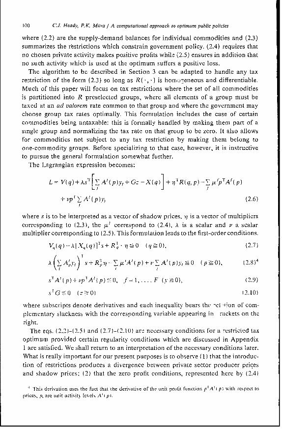
where (2.2) are the supply-demand balances for individual commodities and (2.3)summarizes the restrictions which constrain government policy. (2.4) requires thatno chosen private activity makes positive profits while (2.5) ensures in addition thatno such activity which is used at the optimum suffers a positive loss.
The algorithm to be described in Section 3 can be adapted to handle any taxrestriction of the form (2.3) so long as R(,) is hom.+teneous and differentiable.Much of this paper will focus on tax restrictions where the set of all commoditiesis partitioned into R preselected groups, where all elements of a group must betaxed at an ad valorem rate common to that group and where the government maychoose group tax rates optimally. This formulation includes the case of certaincommodities being untaxable: this is formally handled by making them part of asingle group and normalizing the tax rate on that group to be zero. It also allowsfor commodities not subject to any tax restriction by making them belong toone-commodity groups. Before specializing to that case, however, it is instructiveto pursue the general formulation somewhat further.
The Lagrangian expression becomes:
L =V(q)+AsI[y,Ai(p)yf +Gz-X(q)]+ 7 rR(q, p)- tLtpTA'(p)
+ p r A`( p)v1 (2.6)
where s is to be interpreted as a vector of shadow prices, -q is a vector of multiplierscorresponding to (2.3), the utl correspond to (2.4), A is a scalar and v a scalarmultiplier corresponding to (2.5). This formulation leads to the first-order conditions.
V,(q)A[-A q(q)] ts+ R"q - 77 0 (q 0), (2.7)
A(\ Ap)NR7 L 'P+' A'(Py,< (P=-°) (.)
SrAI(p)+ vp'A'(p)()_, t= 1. F (1-0), (2.9)
s' G c5- ( z ) (2.10)
where subscripts denote derivatives and each inequality bears thte -el tion of com-plementary slackness with the corresponding variable appearing in rackets on theright.
The eqs. (2.2)-(2.5) and (2.7)-(2.l0) are necessary conditions for a restricitcd taxoptimum provided certain regularity conditions which are discussed in Appendix1 are satisfied. We shall return to an interpretation of the necessary conditions later.What is really important for our present purposes is to observe (1) that the introduc-tion of restrictions produces a divergence between private sector producer pricesand shadow prices; (2) that the zero profit conditions, represented here by (2.4)
4 This derivation uses the fact that the derivative of the unit profit function p 'A'( p) with respect toprices, p, are unit activitv levels A'(pt.
CJ. Heady, P.K. Mitra / A computational approach to optimum public policies 101
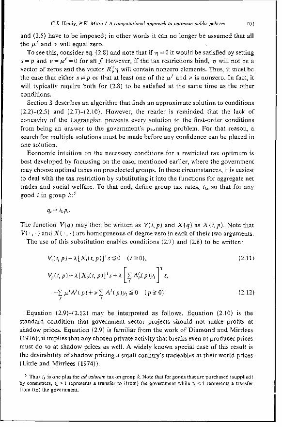
and (2.5) have to be imposed; in other words it can no longer be assumed that all
the ,^Lf and v will equal zero.To see this, consider eq. (2.8) and note that if 77 = 0 it would be satisfied by setting
s = p and -= =0 for all f However, if the tax restrictions bind, X will not be a
vector of zeros and the vector RTT1 will contain nonzero elements. Thus, it must be
the case that either s # p or that at least one of the pkf and v is nonzero. In fact, it
will typically require both for (2.8) to be satisfied at the same time as the otherconditions.
Section 3 describes an algorithm that finds an approximate solution to conditions
(2.2)-(2.5) and (2.7)-(2.10). However, the reader is reminded that the lack of
concavity of the Lagrangian prevents every solution to the first-order conditions
from being an answer to the government's pinning problem. For that reason, a
search for multiple solutions must be made before any confidence can be placed inone solution.
Economic intuition on the necessary conditions for a restricted tax optimum is
best developed by focussing on the case, mentioned earlier, where the government
may choose optimal taxes on preselected groups. In these circumstances, it is easiest
to deal with the tax restriction by substituting it into the functions for aggregate net
trades and social welfare. To that end, define group tax rates, tk, so that for any
good i in group k:5
qi = tk P,-
The function V(q) may then be written as V(t,p) and X(q) as X(t,p). Note that
V(*, * ) and X( , ) are homogeneous of degree zero in each of their two arguments.The use of this substitution enables conditions (2.7) and (2.8) to be written:
V,(t,p)-A[X 1 (t,p)]Ts,O (tO) (:2.11)
Ep t,p -A p( t, p )]Ts +A f ; ys
-' ,uA (p) + BvV A (p)yy_ CO (p 0O). (2.12)
Equation (2.9)-(2.12) may be interpreted as follows. Equation (2.10) is the
standard condition that government sector projects should not make profits at
shadow prices. Equation (2.9) is familiar from the work of Dianmond and Mirrlees
(1976); it implies that any chosen private activity that breaks even at producer prices
must do so at shadow prices as well. A widely known special case of this result is
the desirability of shadow pricing a small country's tradeables at their world prices
(Little and Mirrlees (1974)).
Thus tk is one plus the ad valorem tax on group k Note that for goods that are purchased (supplied)by consumers, rA >J 1 represents a transfer to (from) the government while tk <1 represents a transfer
from (to) the government.

102 CJ. Heady, P.K. Mitra / A computational approach to optimum public policies
Equations (2.11) and (2.12) may be used to generate restricted optimal tax rules.To this end it is best to regard the difference between consumer prices and shadowprices as taxes on consumers, 7, and the difference between producer prices andshadow prices as taxes on private producers, ct. Since shadow prices represent socialopportunity costs, it is natural to think of these differences as capturing the degreeof intervention in consumer and producer decisions respectively. Thus:
r= q-s, co =p-s. (2.13)
Typical eqs. (2.11) and (2.12) may then be written, on using the Slutsky equation,as (disregarding the inequality)
- ~ pi x r~, Z b px-Xj k h j kh , (2.14)
VL p, X, Z p1 X,*sk is k
£ v%a,,yf E u E Ef j 1' f ti X i h __ _ I __h
f - >+r -tXJ+ 1-AX s (2.15)ZA{yf A YA A zA-{yf x
where k, it will be recalled, is the group index and wherex,-h: the derivative of household h's compensated net demand for good i with
respect to the price of good j;aJ: the derivative of firm f's unit-level output of good i with respect to the price
of good j;Af: amount of the ith good (factor) produced (used) by firm f operating at unit
level;bh: the net social marginal utility of income for household h,
a W ai n aXhG-- + |A v t- iJ vh a Ml h v M I '
with Mh (possibly zero) being the lump sum income of household h.The left hand side of eq. (2.14) expresses the proportionate reduction in the value,
at private-sector producer prices, of compensated demand for the goods in tax groupk that would result from a small equiproportional intensification of consumertaxation if shadow prices remained constant.6 These reductions vary from group togroup, being higher for groups which contain commodities predominantly consumedby households with a low net social marginal utility of income.7
The fact that goods subject to tax restrictions cannot satisfy eq. (2.14) on anindividual, but only on an average, basis implies that some goods will be priced
' This is the many-person equivalent of the index of discouragement obtained by Munk (1980), exceptthat the present formulation aggregates over commodities within each group.
For a similar derivation in the unrestricted case see Atkinson and Stiglitz (1980).
C.J. Head}, P.K. Mitra / A computational approach to optimum public policies 103
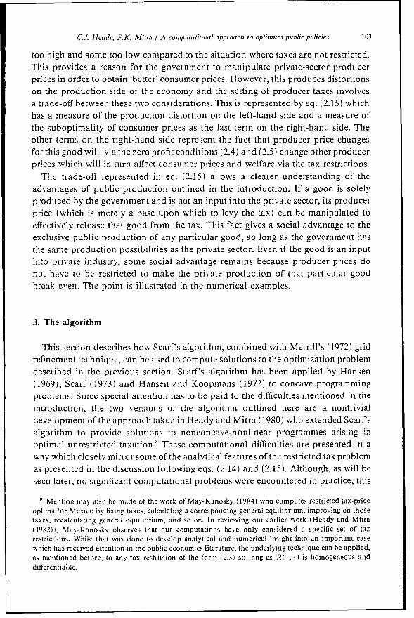
too high and some too low compared to the situation where taxes are not restricted.This provides a reason for the government to manipulate private-sector producerprices in order to obtain 'better' consumer prices. However, this produces distortionson the production side of the economy and the setting of producer taxes involvesa trade-off between these two considerations. This is represented by eq. (2.15) whichhas a measure of the production distortion on the left-hand side and a measure ofthe suboptimality of consumer prices as the last term on the right-hand side. Theother terms on the right-hand side represent the fact that producer price changesfor this good will, via the zero profit conditions (2.4) and (2.5) change other producerprices which will in turn affect consumer prices and welfare via the tax restrictions.
The trade-off represented in eq. (2.15) allows a clearer understailding of theadvantages of public production outlined in the introduction. If a good is solelyproduced by the government and is not an input into the private sector, its producerprice (which is merely a base upon which to levy the tax) can be manipulated toeffectively release that good from the tax. This fact gives a social advantage to theexclusive public pro(luction of anv particular good, so long as the government hasthe same production possibilities as the private sector. Even if the good is an inputinto private industry, some social advantage remains because producer prices donot have to be restricted to make the private production of that particular goodbreak even. The point is illustrated in the numerical examples.
3. The algorithm
This section describes how Scarf's algorithm, combined with Merrill's (1972) gridrefinement technique, can be used to compute solutions to the optimization problemdescribed in the previous section. Scarf's algorithm has been applied by Hansen(1969), Scarf (1973) and Hansen and Koopmans (1972) to concave programmingproblems. Since special attention has to be paid to the difficulties mentioned in theintroduction, the two versions of the algorithm outlined here are a nontrivialdevelopment of the approach takca in Heady and Mitra (1980) who extended Scarf'salgorithm to provide solutions to nonconcave-nonlinear programmes arising inoptimal unrestricted taxation.' These computational difficulties are presented in away which closely mirror some of the analytical features of the restricted tax problemas presented in the discussion following eqs. (2.14) and (2.15). Although, as will beseen later, no significant computational problems were encountered in practice, this
' Mention may also be made of the work of' May-Kanosky (1984) who computes restricted tax-priceoptima for Mexico by fixing taxes, calculating a corresponding general equilibrium, improving on thosetaxes, recalculating general equilibrium, and so on. In reviewing our earlier work (Heady and Mitra(1982)h, Mfav-Kanosklv observes that our computations have only considered a specific set of taxrestrictions. While that was done to develop analytical and numerical insight into an important casewhich has received attention in the public economics literature, the underlying technique can be applied,as mentioned before, to any tax restriction of the form (2.3) so long as R(-, ) is homogeneous anddiflerentiaOile.

104 C'J. Heady, P.K. Mitra / A computational approach to optimum puiblic policies
way of proceeding substantially enhances our understanding of the particulardifficulties that can arise in the restricted tax problem.
The first difficulty is that, if private production is required, the zero profit constraint(2.5) implies that the feasible set has no interior in the (p, t) space over which thealgorithm operates. This means that the grid over which the algorithm searches willnot in general contain any feasible points. Thus, the standard approach, shared byearlier applications of Scarfs algorithm to nonlinear programming problems, ofusing the gradient of the objective function to label feasible points and the gradientof the constraints to label infeasible points can no longer be applied.
One method of dealing with equality constraints is to substitute them out, as wasdone with the tax restrictions. However, this is nov practicable here because theconstraint:
pTAf(p)- = 0 for allf
is not continuous at v, = 0, the second feature discussed earlier in the paper. Thisparticular difficulty could be eliminated if the optimum set of private sector activities(call it L) is known and specified in advance. The complementarity restriction couldthen be transformed into the better behaved restriction:
pT A'(p) 0 for ali fB L, (3.1)
pTAf(p) =0 for all Jfe L. (3.2)
Even if this could be done, substitution would be difficult as the restriction is notat all simple.
For these reasons, the problem is handled differently and the gradient of theobjective function is used in labelling some points in the grid that do not actuallysatisfy all of the feasibility conditions. However, the labelling is modified to ensurethat all the feasibility conditions are satisfied when the algorithm terminates.
Two methods have been used to solve these problems and the results of both ofthem are presented. The first (Approach A) relaxes the zero-profit constraint byallowing small losses to be made. Thus, the algorithm solves a modified problemwith the restriction (2.5) replaced by:
v pTAf(p)yf -_6 (3.3)f
where 6 is a small positive number. The size of these losses can be reduced as thegrid density is increased, so that losses are very small at the limit. In many casesthe solution to the modified problem will be a good approximation to the solutionof the underlying problem, for 6 sufficiently small. This method has the clearadvantage that it simultaneously finds both optimal taxes and optimal public andprivate production. However, it has the disadvantage that the algorithm cannottheoretically be guaranteed to converge to a solution when 6 equals zero, in whichcase the approximation to the underlying problem will not be good. The difficulty

C.J. Headly, P.K. Mitra / A computational approach to optimum public policies 105
might arise if the solution to the modified problem includes a yf which is positivewhen the correct solution has that y, equal to zero. The solution to the modifiedproblem will then satisfy first-order conditions which include terms in that unwantedactivity. However, even after running a large number of examples, this problemremains to be encountered in practice and Approach A has proved capable oflocating an approximate solution to the first order conditions for a restricted taxoptimum.
The second method (Approach B) avoids the possible difficulties of Approach Aby specifying in advance the set (L) of private sector activities that are used at theoptimum. In this approach the zero profit constraints are ignored in assessingfeasibility but the labelling is modified to ensure that all the activities in L makezero profit (and the others make nonpositive profits) at the point where the algorithmterminates. The rationale behind Approach B is that it is often fairly easy to makean educated guess as to which private sector activities will be used at the optimum.For example, in a number of countries the government appropriates for itself the.commanding heights' of the economy, leaving the rest of manufacturing activity toth., private sector. Thus, there is very little choice as to which goods are producedprivately. Even when this is not the case, observation of the relative efficiencies ofpublic and private production in different industries might give a good idea of whichindustries should include private firms. In these circumstances, it is unnecessary touse the more complex Approach A and Approach B should be used.
The possibility of altering L gives Approach B a role even when the compositionof the set L is difficult to guess a priori: that of checking whether Approach A hasindeed found a global rather than a local optimum. This can be useful because theinherent nonconcavity of the optimal tax problem is exacerbated in the restrictedtax case by the indivisibility associated with the complementary slackness restriction.Thus, Approach A might find a solution to the first-order conditions involving aprivate production activity that is worthwhile given that its zero-profit conditionmust be satisfied, but which should be abandoned if its zero-profit condition couldalso be dropped. This possibility can be checked with Approach B by removing thesuspect activity from the set L. This point will be illustrated in the numerical examplesof Section 4.
Finally, mention may be made of the fact that Approach B can be used on itsown if Approach A does indeed encounter difficulties as 5 is reduced to zero). Insuch a case several computer runs can be used, each with a different set of L, andthe solution with the highest social wtI'aIre chosen. Hiowever, as stated above, thisparticular difficultv with Approach A has never arisen in our computationalexperience.
Labelling rules
We turn now to a description of the computational procedures. Since demandand supply functions are homogeneous of degree zero in both the private producer

106 C.J. Heady, P.K. Mitra / A computational approach to optimum public policies
prices p and the group tax rates t, we may normalize those variables to lie on the(n + R)-dimensional unit simplex S, + R, i.e.,
pT e, +tT eR =1 (3.4)
where ef denotes an M-column vector of unit entries.9 The Scarf algorithm is thenused to conduct a systematic search on S, + R.
The structure and argument underlying the two approaches are very similar. Wedescribe them below for A and later indicate precisely what changes are needed forB. Section 4 reports on the experiernce of using both approaches. Convergenceproperties for both algorithms are established in Theorems (A.2) and (A.3) ofAppendix 1.
Approach A
The rules used in Approach A to associate each element of the grid of vectorsI. 1.... 1k in Sn + R with an (n + R) dimensional column vector, b, are as follows.
(1) For a vector I containing its first zero clement in the jth position, b is givenby l ', the jth unit vector (j = 1, . .. , n + R).
(2) For all vectors not covered by rule (1) and for which
p enG_-0.4, h=eo)
(3) For all vectors not covered by rule (1) and for which
tTeR < 0.4, b = (
All other vectors are labelled as follows(4) If PTA-(p) > Q for somef
IA/
(5) If p1 A'(p) (, we calculate X(t, p) the vector of aggregate net trades. Twocases need to be distinguished.
(i) if X( t, p) satisfies the feasibility requirement:
v A'(p)yt+Gz-X(t,p)_O, b= eR+ V,.
' This normalization implies, since t is a v ector of one plus ad valoremil tax rates, that q - p. However,q< p, which implies nonnegative government subsidies all round, does not necessarily lead to a budgetdeficit. See footnote 5.

CJ. Heady, PK. Mitra / A computational approach to optimum public policies 107
(ii) If X(t, p) fails to satisfy the market clearance inequalities:
en + [E Af yf -XP]s+ E A'yj
b = ( ~+ [z _ XTs
The test of feasibility and the values (s, 'k, yf) are furnished by a pair of parametricprogrammes: for each (p, t) covered by rule (5) choose (s, k) to maximize
sTX _, (P)
subject to
(s + OP )A-f + Opt-: O for all f,
sTG ' O
s en+0=1, s,O-k-O,
and its dual: choose (w, yf, z) to minimize
w (P)
subject to
_Atvf+Gz+we, X,.f
(PTAfJ+ EJ)V X+ w -8,
Z -> 0.
In the programmes, 8 (>0) represents the permissible total loss from (3.3). TheFf (>O) represent permissible unit losses for each activity over and above the totalloss 8. The ej can be reduced to zero as the grid becomes infinitely dense so that(3.3), which bounds the total loss, is satisfied in the limit.
Rule (1) above associates unit vectors with the sides of Sn + R. Rule (2) [resp.(3)] is introduced to prevent difficulties that can arise with the definitions of theprivate sector's responses if all producer prices [resp. tax rates] go to zero. Rule (5)is directed at satisfying the first order conditions (2.11) and (2.12). The linearprogrammes (P) are of considerable economic interest as well. The dual minimizesthe largest deviation between demand and supply while attempting an approximatefulfillment of the zero profit conditions.
Approach B
In this approach labelling rules (1)-(4) remain unchanged. Rule (5) is altered to:(5') if pTA] (p) 'O0, we calculate X. Two cases need to be distinguished:(i) if X satisfies the feasibility requirement
eR + Vp+EA
b= eR + VI
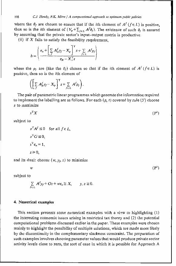
108 C.J Heady, P.K. Mitra / A computational approach to optimum public policies
where the Of are chosen to ensure that if the ith element of Af (fe L) is positive,
then so is the ith element of (VI +JfCL Af61). The existence of such 0j is assured
by assuming that the private sector's input-output matrix is productive.(ii) if X fails to satisfy the feasibility requirement,
I el+ZA'fXl Ts+ > Afp~.|en, + [ AYf Xp]s f vPf
bLf J f c L )eR-Xt S
where the pf are (like the 0,) chosen so that if the ith element of Af (f E L) is
positive, then so is the ith element of
([AJyf_xp1TS+zY Af'pf)
The pair of parametric linear programmes which generate the information required
to implement the labelling are as follows. For each (p, t) covered by rule (5') choose
s to maximize
ST X (PI)
subject to
sTA" ' O for all fE L,
STG 0,
sTe
s -- = ,smO,
and its dual: choose (w, yf, z) to minimize
w (P')
subject to
Afyf+Gz+ we,_ X, y, z >0.
4. Numerical examples
This section presents some numerical examples with a view to highlighting (1)
the interesting economic issues arising in restricted tax theory and (2) the potential
computational problems discussed earlier in the paper. These examples were chosen
mainly to highlight the possibility of multiple solutions, which are made more likely
by the discontinuity in the complementary slackness constraint. The preparation of
such examples involves choosing parameter values that would produce private sector
activity levels close to zero, the sort of case in which it is possible for Approach A
CJ. Heady, PK. Mitra / A computational approach to optimum public policies 109
to run into difficulties. However, despite the use of Approach A in about forty cases,this problem was never encountered.
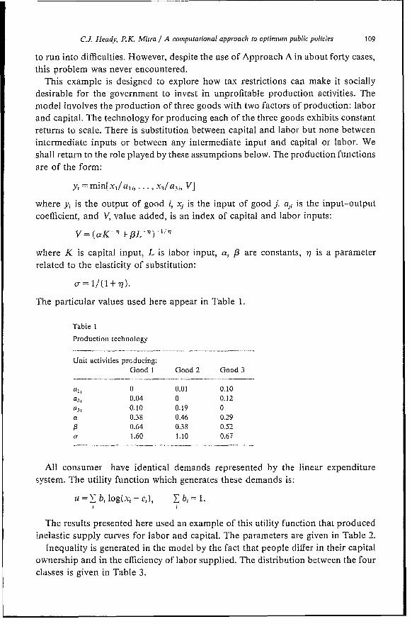
This example is designed to explore how tax restrictions can make it sociallydesirable for the government to invest in unprofitable production activities. Themodel involves the production of three goods with two factors of production: laborand capital. The technology for producing each of the three goods exhibits constantreturns to scale. There is substitution between capital and labor but none betweenintermediate inputs or between any intermediate input and capital or labor. Weshall return to the role played by these assumptions below. The production functionsare of the form:
y, = min[x/ a, j.., X 3/ a3 1 V]
where yi is the output of good i, xj is the input of good j. aji is the input-outputcoefficient, and V, value added, is an index of capital and labor inputs:
V= (aK-77 +,L--' ) - 1 T1
where K is capital input, L is labor input, a, ,B are constants, 'q is a parameterrelated to the elasticity of substitution:
o- = 1/(1 + X ).
The particular values used here appear in Table 1.
Table 1
Production technology
Unit activities producing:Good 1 Good 2 Good 3
al, 0 0.01 0.10a2, 0.04 0 0.12a3 , 0.10 0.19 0a 0.38 0.46 0.29,B 0.64 0.38 0.52Cr 1.60 1.10 0.67
All consumer have identical demands represented by the linear expendituresystem. The utility function which generates these demands is:
u = b, log( xi -c e), bi =- 1.
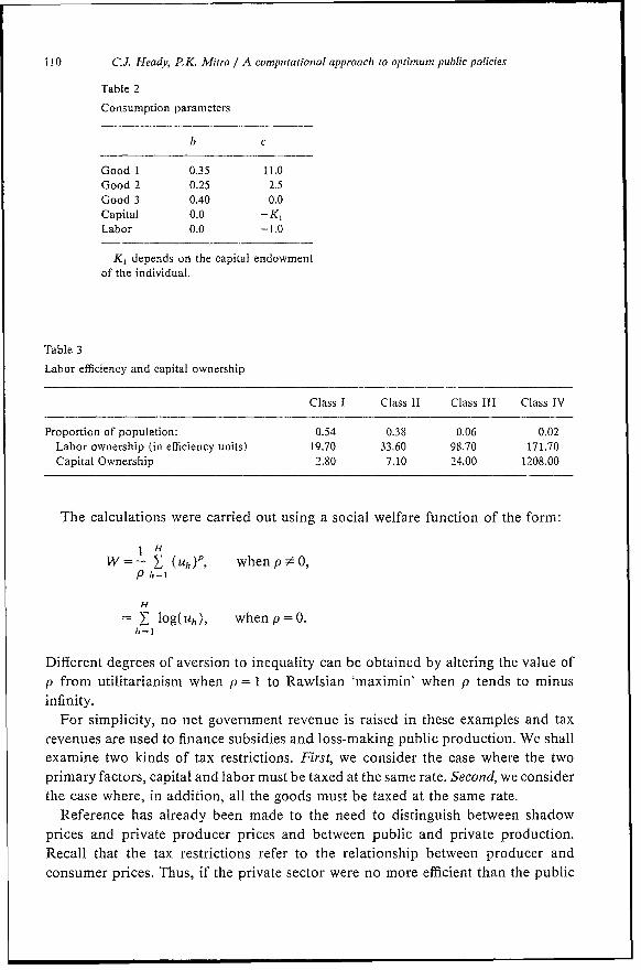
T'he results presented here used an example of this utility function that producedinelastic supply curves for labor and capital. The parameters are given in Table 2.
Inequality is generated in the model by the fact that people differ in their capitalownership and in the efficiency of labor supplied. The distribution between the fourclasses is given in Table 3.
110 C.J. Heady, P.K. Mitra / A computational approach to optimum public policies
Table 2
Consumption parameters
b c
Good 1 0.35 11.0Good 2 0.25 2.5Good 3 0.40 0.0Capital 0.0 -K,Labor 0.0 -1.0
K, depends on the capital endowmentof the individual.
Table 3
Labor efficiency and capital ownership
Class I Class 11 Class III Class IV
Proportion of population: 0.54 0.38 0.06 0.02Labor ownership (in efficiency units) 19.70 33.60 98.70 171.70Capital Ownership 2.80 7.10 24.00 1208.00
The calculations were carried out using a social welfare function of the form:
l HW=- E (uh)P, whenp$ O,
P h=l
H
= log(1uh), when p = O.h-1
Different degrees of aversion to inequality can be obtained by altering the value ofp from utilitarianism when p= 1 to Rawlsian 'maximin' when p tends to minusinfinity.
For simplicity, no net government revenue is raised in these examples and taxrevenues are used to finance subsidies and loss-making public production. We shallexamine two kinds of tax restrictions. First, we consider the case where the twoprimary factors, capital and labor must be taxed at the same rate. Second, we considerthe case where, in addition, all the goods must be taxed at the same rate.
Reference has already been made to the need to distinguish between shadowprices and private producer prices and between public and private production.Recall that the tax restrictions refer to the relationship between producer andconsumer prices. Thus, if the private sector were no more efficient than the public
C.J. Heads; P.K. Mitra / A computational approachi to optimum public policies
sector, all production would be in public hands because this would circumvent the
tax restrictions. To avoid this, it is assumed that the government can obtain only a
certain percentage of the efficiency of the private sector: the index of efficiency, as
represented by a shift parameter outside the production function is the same for all
three industries. It is then interesting to ask how much public production, relative
inefficiency notwithstanding, the furtherance of redistributive objectives requires
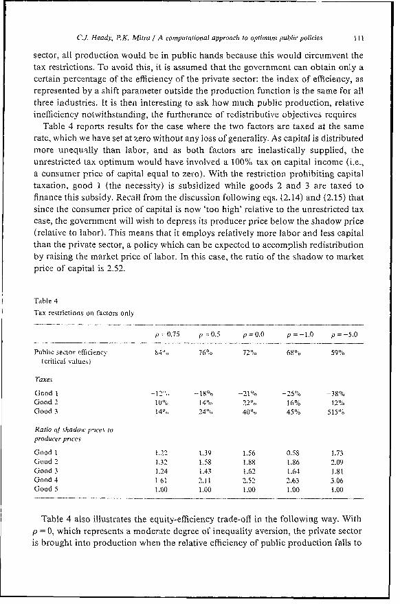
Table 4 reports results for the case where the two factors are taxed at the same
rate, which we have set at zero without any loss of generality. As capital is distributed
more unequally than labor, and as both factors are inelastically supplied, the
unrestricted tax optimum would have involved a 100% tax on capital income (i.e.,
a consumer price of capital equal to zero). With the restriction prohibiting capital
taxation, good I (the necessity) is subsidized while goods 2 and 3 are taxed to
finance this subsidy. Recall from the discussion following eqs. (2.14) and (2.15) that
since the consumer price of capital is now 'too high' relative to the unrestricted tax
case, the government will wish to depress its producer price below the shadow price
(relative to labor). This means that it employs relatively more labor and less capital
than the private sector, a policy which can be expected to accomplish redistribution
by raising the market price of labor. In this case, the ratio of the shadow to market
price of capital is 2.52.
Table 4
Tax restrictions on factors only
p O.75 p = 0.5 p - 0.0 p = -1.0 p -S5.0
Public sector efficiencv t 76% 72; 68% 59%
(critical values)
Taxes
Good 1 12" -18% -21% -25% - 38 0/
Good 2 10()° 14% 22% 16% 12%.o
Good 3 14% 24'% 40% 45°% 515%°
Ratio ol shadov prices toproducer prices
Good 1 1.22 1.39 1.56 0.58 1.73
Good 2 1.32 1.58 1.88 1.86 2.09
Good 3 1.24 1.43 1.62 1.64 1.81
Good 4 1.61 2.11 2.52 2.63 3.06
Good 5 1.00 1.00 1.00 1.00 1.00
Table 4 also illustrates the equity-efficiency trade-off in the following way. With
p = 0, which represents a moderate degree of inequality aversion, the private sector
is brought into production when the relative efficiency of public production falls to
112 C.J. Headv, P.K Mitra / A computational approachl to optimum public policies
72%. The higher degree of aversion to inequality, say, the lower the critical valueof the public-private efficiency index before private production is allowed. Giventhat the sole purpose of taxation is redistributive, the economy is prepared to giveup more and more efficiency for the sake of circumventing restrictions on its abilityto tax. The ratio of the shadow to market price of capital also moves in the expecteddirection.
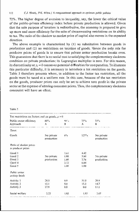
The above example is characterized by (1) no substitution between goods inproduction and (2) no restrictions on taxation of goods. Hence the only role forproducer prices of goods is to ensure that private sector production breaks even.This guarantees that there is no social cost to satisfying the complementary slacknesscondition on private production; its Lagrangian multiplier is zero. For this reason,its discontinuity at v = 0 causes no potential difficulties for computation. To illustratethis particular difficulty, it is necessary to introduce a tax restriction on the goods.Table 5 therefore presents where, in addition to the factor tax restriction, all thegoods must be taxed at a uniform rate. In this case, because of the tax restrictionon the goods, producer prices can only be set to achieve zero profit in the privatesector at the expense of altering consumer prices. Thus, the complementary slacknessconstraint will have an effect.
Table 5
Tax restrictions on factors and on goods, ,- 0
Public sector efficiency 80X, 73°O 739oApproach A B A B
Taxes
Goods No private 0% 127"A No privateproduction production
Ratio of shiadow pricesto producer prices
Good 1 1.61 4.42Good 2 No private 1.90 3.80 No privateGood 3 production 1.68 2.76 productionGood 4 2.72 6.84Good 5 1.00 1.00
Public sectoractivitv levels
Activity 1 29.0 0.() 31.0 29.9Activity 2 15.1 O.0 15.3 14.7Activity 3 17.9 (1.0 0.0 17.1
Social welfare 2.22 1.93 1.95 2.07
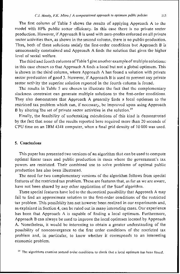
C.J. Heady, P.K. Mitra / A computational approach to optimum public policies 113
The first column of Table 5 shows the results of applying Approach A to themodel with 80% public sector efficiency. In this case there is no private sectorproduction. However, if Approach B is used with zero-profits enforced on all privatesector activities then, as shown in the second column, there is no public production.Thus, both of these solutions satisfy the first-order conditions but Approach B isunnecessarily constrained and Approach A finds the solution that gives the higherlevel of social welfare.
Thethirdand fourth columns of Table 5 give anotherexampleofmultiplesolutions:in this case chosen so that Approach A finds a local but not a global optimum. Thisis shown in the third column, where Approach A has found a solution with privatesector production of good 3. However, if Approach B is used to prevent any privatesector actil ity the superior solution reported in the fourth column is found.
The results in T'able 5 are chosen to illustrate the fact that the complementaryslackness constraint can generate multiple solutions to the first-order conditions.They also demonstrate that Approach A generally finds a local optimum to therestriceed tax problem which can, if necessary, be improved upon using ApproachB by altering 'the set of private sector activities in the solution."'
Finally, the feasibility of undertaking calculations of this kind is demonstratedby the fact that none of the results reported here required more than 20 seconds ofCPU time on an IBM 4341 computer, when a final grid density of 10 000 was used.
5. Conclusions
This paper has presented two versions of an algorithm that can be used to computeoptimal linear taxes and public production in cases where the government's taxpowers are restricted. Their combined use to solve problems of optimal publicproduction has also been illustrated.
The need for two complementary versions of the algorithm follows from specialfeatures of the restricted tax problem. These are features that, as far as we are aware,have not been shared by any other application of the Scarf algorithm.
These special features have led to the theoretical possibility that Approach A mayfail to find an approximate solution to the first-order conditions of the restrictedtax problem. This possibility has not however been realized in our experiments and,as explained in Section 4, can be ruled out in many interesting cases. Our experiencehas been that Approach A is capable of finding a local optimum. Furthermore,Approach B can always be used to improve the local optimum located by ApproachA. Nonetheless, it would be interesting to obtain a greater understanding of thepossibility of nonconvergence to the first order conditions of the restricted taxproblem and, in particular, to know whether it corresponds to an interestingeconomic problem.
"' The algorithms examine second order conditions to check that a local optimum has been found.

114 C.J. Heady, P.K. Mitra / A computational approach to optimum public policies
Appendix 1
The rules of association for both Approaches A and B lead to a matrix B whosecolumns correspond to the grid vectors I ....., l'.
I1 12 ln+R in+R+1 . . . Ik
-1
0 0 bi..+r b.* blk
B 0 1 * 0 b2 ,n+R+l b2k
n0 0 * 1 bI++R1 t- n+R,k-
The theorem which uniderlies Scarf s algorithm states;
Theorem A.1. Let li be associated with the jth column of the matrix B. Assume thatthe set of nonnegative solutions to the equations Bc = en+r is bounded. Then thereexists a primitive set lI, . . , P'-"i such that the columns ji, . . .,Jn+R form a feasiblebasis for Bc = e + R (i.e., these equations have a nonnegative solution, where c1 O fori Oil, * * * .in+R)-
This theorem may be used to solve our problem if it can be shown that theboundedness condition on which it relies is satisfied here. Consider a typical rowof the matrix B. The units in which social welfare (resp. goods) are measured canbe chosen so that the entries for any row under labelling rule 5(i) and 5'(i) [resp.(ii)] are positive for all (p, t). This bounds the weights c of the above theorem thatare associated with columns generated by rules (5) and (5'). This fact, together withthe assumption that some inputs are required to produce any output, also boundsthe weights associated with columns generated by rule (4). As all other entries inB are nonnegative, the boundedness condition is satisfied.
We first show for Approach A that the primitive set whose columns form a feasiblebasis for Bc = ef+R defines an approximate solution to the first order conditions fora restricted tax optimum, modified by allowing small losses, provided a certainregularity condition is satisfied.
We begin by stating the regularity condition (REG) which plays a role analogousto that of a constraint qualification in nonlinear programming.
Regularity Condition (REG): There do not exist vectors (p, q, s) (p, q, s • 0) wheres satisfies the programme (P) such that sTX 2 0 and
(XI) Ts -0 ( t 30). (A. 1)
The condition is very similar to the one introduced and interpreted in Heady andMitra (1980). We therefore confine ourselves to noting that the condition hassubstantial economic content. The regularity condition states that whenever thevalue of aggregate net trades is nonnegative at shadow prices, there exists a directionof movement in taxes which decreases the value of aggregate net trades measured
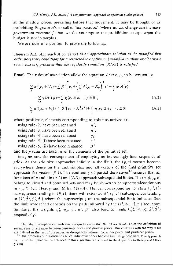
C.J. Heady, P.K. Mitra / A computational approach to optimum public policies 115
at the shadow prices prevailing before that movement. It may be thought of asprohibiting Edgeworth's so-called 'tax paradox' (where no tax change can increasegovernment revenue),"' but we do not impose the prohibition except when thebudget is not in surplus.
We are now in a position to prove the following:
Theorem A.2. Approach A converges to an approximate solution to the modified firstorder necessary conditions for a restricted tax optimum (modified to allow small privatesector losses), provided that the regularitY condition (REG) is satisJied.
Proof. The rules of association allow the equation Bc =-- e,,; R to be written as:
v i[e+V)+ E [ e, + ( At Y -- ,Yp s' +V JA']
y f yA'( p )+ 77,eie,= e,, p 0>), (A.2)
a' [eR-t V,]- [3[eR-X,s ]+) 7eRn eR (t->0) (A.3)
where positive c, elements corresponding to columns arrived at:using rule (2) have been renamedusing rule (3) have been renamedusing rule (4) have been renamed ,,using rule (5) (i) have been renamed a'',using rule (5) (ii) have been renamed ,B'
and the j-sums are taken over the elements of the primitive set.Imagine now the consequences of employing an increasinglv finer sequence of
grids. As the grid size approaches infinity in the limit, the (p, t) vectors becomeeverywhere dense on the unit simplex and all vectors of the final primitive setapproach the vector 'p t). The continuity of partial derivatives' 2 ensures that allfunctions of p and t in (A.2) and (A.3) approach subsequential limits. The (s5, !,v, z)belong to closed and bounded sets and may be shown to be uppersemicontinuousin (p, t) (cf. Heady and Mitra (1980)). Hence, corresponding to each (p', t')subseqtuence tending to (j$, t), there will exist (s", 03, v-', z') subsequences tendingto (.' ',4i, l') where the superscript j on the subsequential limit indicates thatthe limit aproached depends on the path followed by the (s', ;0', yl, zj) sequence.Similarly, the weights -, 7, y,', a', ,B' also tend to limits (J.' , ,I)respectively.
'1 One slight complication with this interpretation is that the 'taxes' which enter the definition ofrevenue are divergences between consumer prices and shadow prices. This contrasts with the way taxesare definied in the rest of the paper, as divergences between consumer prices and producer prices.
12 The problems of discontinuity when individual prices become small is ignored here. One approachto this problem, that can be extended to this algorithm is discussed in the Appendix to Heady and Mitra(1980).

116 C.J Headv, P.K. Mitra / A computational approach to optimum public policies
At the subsequential limits, (A.2) and (A.3) may be written as:
&[e+n P ] E _ en ( L' A P ' JA ) Af
ff- yf. Af + 7,e en e P 0- ), (A-4)J'
&[eR + V]+ 3 eR-Xt s]+ 2eR -eR (t-O) (A.5)
where
It needs to be shown that the subsequential limits satisfy the modified first orderconditions for the planning problem. Accordingly, the proof argues (1) that all unit(i.e., en-type) entries in (A.4) and (A.5) may be eliminated, (2) that each of thesubsequential limits (Si7', 2Q- --i) may be averaged using the weights J and (3)that a > 0, a result that implies all the first order conditions are satisfied.
Step (1). Suppose p,en < 0.4. Then 7j > 0 and i 2 = yJ = a = /' vi . (A.5) reads
('0).(X >)
Since tTeR = 0.6, not all ti are zero and the above violates complementary slackness.Hence, PTTen 2 0.4. Similarly, the supposition that ?TeR < 0.4 violates complementaryslackness, this time using (A.4). Hence, tTreR - 0.4.
Next multiply (A.4) (resp. (A.5)) by p (resp. F) and sum the n (resp. R) equations.Homogeneity of degree zero of demand and supply functions in p and t, together
with the earlier assurance that 'Te,, $ 0 and tTeR $ 0 yields
a+f3-+'q2-1. (A.7)
Subtract (A.7) from (A.6) to get
p2) = [ PT j f (A.8)
From the labelling rules (4) and (5), 5 f> 0 implies pTAf>0 and /j > 0 impliesITAf - 0, all f Hence the right hand side of (A.8) is nonnegative, i.e., j 11 27. Butinspection of labelling rules (2) and (3) reveals that 1 and 72 cannot both be

C.J. Heady, P.K. Mitra / A computational approach to optimum public policies 117
positive. Therefore r2 =0, whence (A.7) and (A.8) may be written
c ,l ji -1, (A.9)j
iFi
Since cx +>Yj ,Bi = 1, it is clear from the labelling rules (5) that pTAf O, all Fromthe parametric programme (P), at the limit where e 0 0 for all f:
Y jfpTAffj =- i (8 +
Hence
A T I i,B ( + ) (A. 11)
where we have used the fact that P Te, - 0.4. The size of 7, therefore depends onthe value of 8 to which we shall return presently. Meanwhile, eqs. (A.4) and (A.5)may be simplified to:
a: VP + T [( A-, f) + vfij
- A+ 77lefl-0 ( P 0 °0), (A. 12)
ceVt-< 'X'.s}< O t O)(A. 13)
where (A.7) and (A.11) hold true.Step (2). Equations (A.13) imply that so long as there exists some group of
commodities, r (possibly consisting of just one good), a rise in whose tax rate
improves social welfare, i.e., O) V/ltr > 0, it cannot be the case that ,3.' = 0, all j. Themonotonicity assumption of the previous sentence would be satisfied, for example,by a tax rate on a group consisting of different (or possibly one) kinds of labor ifconsumers appear solely as suppliers. Then define ,B and
A j t A/3 7 /3o -1'
Equations (A. 12 and i A.13) now simplify to:
A Ai ,e, 0 -$T O(,O ) (A. 14)
c~§PT~ t~ (A. 15)
118 C8.J. Heady, P.K. Mitra / A computational approach to optimum public po,icies
where
A 1 AA
l , O 1 04 ,(0 + 8). (A.16)
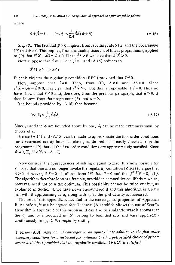
Step (3). The fact that /3 > 0 implies, from labelling rule 5 (ii) and the programme(P) that w - 0. This implies, from the duality theorem of linear programming appliedto (P) that sk - +5 = i > 0. Since k8 - 0 we have that gTX - 0.
Next suppose that 0 =0. Then :3 = 1 and (A.15) reduces to
But this violates the regularity condition (REG) provided that s • 0.Now suppose that g = 0. Then, from (P), k 50 and d, > 0. Since
sTX -_48 = w _ 0, it is clear that gTX > 0. But this is impossible if s = 0. Thus wehave shown that s # 0 and, therefore, from the previous paragraph, that a > 0. Itthen follows from the programme (P) that iw = 0.
The bounds provided by (A.16) then become
10 0 -fi:5 (A.17)
Since :3 and the b are bounded above by one, a, can be made extremely small bychoice of 8.
Hence (A.14) and (A.15) can be made to approximate the first order conditionsfor a restricted tax optimum as closely as desired. It is easily checked from theprogramme (P) that all the first order conditions are approximately satisfied. Since
Now consider the consequences of setting 8 equal to zero. It is now possible tors= 0, so that one can no longer invoke the regularity condition (REG) to argue that& > 0. However, if s = 0, if follows from (P) that iw =0 and that pTA. tQ = 0, all fThe algorithm therefore locates a feasible, tax-ridden competitive equilibrium which,however, need not be a tax optimum. This possibility cannot be ruled out but, asexplained in Section 4, we have never encountered it and this algorithm is alwaysrun with 8 approaching zero, along with Fy; as the grid density is increased.
The rest of this appendix is devoted to the convergenice properties of ApproachB. As before, it can be argued that Theorem (A.1) which allows the use of Scarf'salgorithm is applicable to this problem. It can also be straightforwardly shown thatthe 0, and pt introduced in (5') belong to bounded sets and vary uppersemi-continuously in (p, t). We begin by stating
Theorem (A.3). Approach B converges to an approximate solution to the first ordernecessary conditionsfor a restricted tax optimum (with a prespecafied choice of privatesector activities) provided that the regularity condition (REG) is satisfied.

C.J. Heady, P.K. Mitra / A computational approach to optimum public policies 119
Proof (sketch). We shall concentrate only on those features of the proof which aredifferent from that of Theorem A.2.
Thus, at the subsequential limit we have
c en±Vp+ f Aft ] + [en + ( Afyf -p) B + E AfPf]
- y A± + -q7e e (I P-0) (A.18)I
ci [R +V,] ,i[eRX, S + 72e eR t 0)(A.l19)
where the j superscripts have been omitted for simplicity; the omission, it will berecalled, is justified by Step (2) of the proof.
Step (1). The argument is as before except that we also show that 6TAf= 0, for
all fe L. Multiplying (A.18) and (A.19) by (p, t) and exploiting homogeneity, wehave:
aF[1fl + [ 1+P A f |- + I1 (A.20)
a + + i= 1 . (A.21)
Subtract (3.25) fron (3.24) to get
(+ +2) pTe[£ 9fP A - &i$ T o3 A'Of- Op *1 (A.22)fi nf f J
The argument used below (A.8) shows that the right hand side of (3.26) is nonnegativefrom which it follows that ' 2 =0. Equations (A.21) and (A.22) then simplify to
a +, (A.23)
1 IF A- _ Sp,,A f_~Ty'f77 l e [ ciJ3 > AJ-fi'>3 A'pf I. (A.24)pe.Lf f f J
(A.23) implies that pTTA-0. Suppose one of these inequalities to be strict and let,>0. Equation (A. 18) may be rearranged, using (A.24), to yield:
P+^ ] 3 AOfy - s+ Af P >- yA <O*p(*f,13 v ) AP f,I>3fAf<0. (A.25)ffL L\ / fc L Jf
Let the private industry producing good i bz the one which suffers losses. Considerthen the ith equation in (A.25). The first two terins are strictly positive by construc-tion. As industry i is making a loss, the third term is nonpositive. Hence the lefthand side cannot be strictly negative as (A.25) would require. Thus AlTAf = 0 for all
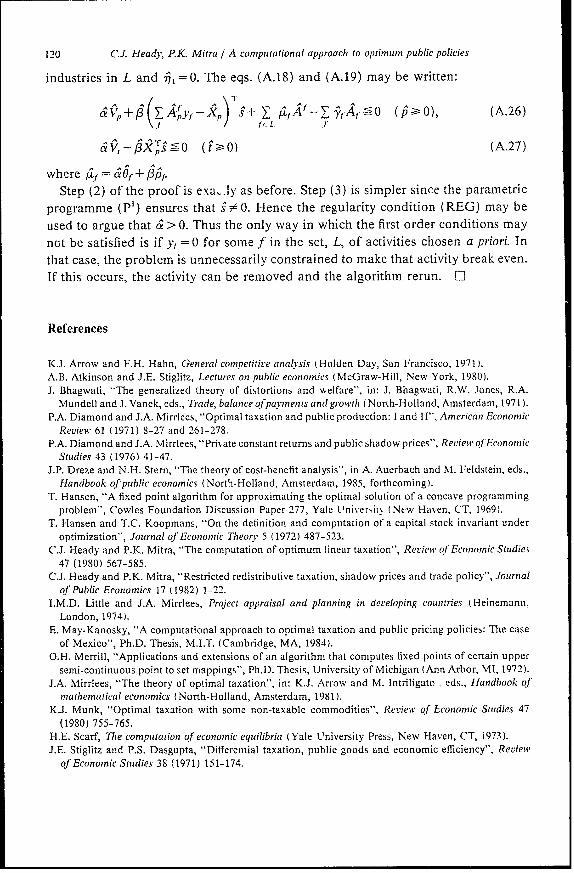
120 CJ. Heady, P.K. Mitra / A computational approach to optimum public policies
industries in L and i1.=O. The eqs. (A.18) and (A.19) may be written:
a; k 3(E4t p ) ;y1A ( p-2 0 ),(A.26)
a Tg X O (Nt 0) (A.27)
where bLt = Of+fpf
Step (2) of the proof is exaJ.y as before. Step (3) is simpler since the parametricprogramme (P') ensures that s.O 0. Hence the regularity condition (REG) may beused to argue that a > 0. Thus the only way in which the first order conditions maynot be satisfied is if yt, = 0 for some f in the set, L, of activities chosen a priori. Inthat case, the problem is unnecessarily constrained to make that activity break even.If this occurs, the activity can be removed and the algorithm rerun. O
References
K.J. Arrow and F.H. Hahn, General competitive analysis (Holden Day, San Francisco, 1971).A.B. Atkinson and J.E. Stiglitz, Lectures on public economic's (McGraw-Hill, New York, 1980).J. Bhagwati, "The generalized theory of distortions and welfare", in: J. Bhagwati, R.W. Jones, R.A.
Mundell and J. Vanek, eds., Trade, balance of pavnents andgrowth (North-Holland, Amsterdam, 1971).P.A. Diamond and J.A. Mirrlees, "Optimal taxation and public production: I and 11", American Economic
Review 61 (1971) 8-27 and 261-278.P.A. Diamond and J.A. Mirrlees, "Private constant returns and public shadow prices", Review ol Econornic
Studies 43 (1976) 41-47.J.P. Dreze and N.H. Stern, "The theory of cost-benefit analysis", in A. Auerbach and M. Feldstein, eds.,
Handbook ofpublic economics (North-Holland, Amsterdam, 1985, forthcoming).T. Hansen, "A fixed point algorithm for approximating the optimal solution of a concave programming
problem", Cowles Foundation Discussion Paper 277, Yale lUniver-ir, (New Haven, CT, 1969).T. Hansen and T.C. Koopmans, "On the definition and computation of a capital stock invariant under
optimization", Journal ot Economic Thaeor.y 5 (1972) 487-523.C.J. Heady and P.K. Mitra, "The computation of optimum linear taxation", Review of Economic Studies
47 (1980) 567-585.C.J. Heady and P.K. Mitra, "Restricted redistributive taxation, shadow prices and trade policy", Journal
of Public Economics 17 (1982) 1-22.I.M.D. Little and J.A. Mirrlees, Project appraisal and planning in developing countries (Heinemann,
London, 1974).E. May-Kanosky, "A computational approach to optimal taxation and public pricing policies: The case
of Mexico", Ph.D. Thesis, M.I.T. (Cambridge, MA, 1984).O.H. Merrill, "Applications and extensions of an algorithm that computes fixed points of certain upper
semi-continuous point to set mappings", Ph.D. Thesis, University of Michigan (Ann Arbor, MI, 1972).J.A. Mirrlees, "The theory of optimal taxation", in: K.J. Arrow and M. Intriligato . eds., Handbookl of
mathematical economics (North-Holland, Amsterdam, 1981).K.J. Munk, "Optimal taxation with some non-taxable commodities", Review of Ecotnomic Studies 47
(1980) 755-765.H.E. Scarf, Thae computation of economic equilibria (Yale LUniversity Press, New Haven, CT, 1973).J.E. Stiglitz and P.S. Dasgupta, "Differential taxation, public goods and economic efficiency", Review
of Economic Studies 38 (1971) 151-174.