Public Debt and Low Interest Rates

Olivier Blanchard ∗

September 24, 2018 – Version 1

∗Peterson Institute for International Economics and MIT (oblanchard@piie.com) Pre-liminary. Do not quote. AEA Presidential Lecture, to be given in January 2019. Spe-cial thanks to Larry Summers for many discussions and many insights. Thanks for com-ments, suggestions, and data to Simcha Barkai, Charles Bean, Philipp Barrett, John Camp-bell, John Cochrane, Carlo Cottarelli, Peter Diamond, Stanley Fischer, Francesco Giavazzi,Larry Kotlikoff, Lorenz Kueng, Thomas Philippon, Jim Poterba, Robert Solow, Jaume Ven-tura, Philippe Weil, Jeromin Zettelmeyer, and my PIIE colleagues. Thanks for outstandingresearch assistance to Thomas Pellet, Colombe Ladreit, and Gonzalo Huertas.

2

Abstract

The lecture focuses on the costs of public debt when safe interest

rates are low. I develop four main arguments.

First, I show that the current situation in which, in the United States,

safe interest rates are expected to remain below growth rates for a long

time, is more the historical norm than the exception. If the future is

like the past, this implies that debt rollovers, that is the issuance of debt

without a later increase in taxes may well be feasible. Put bluntly, public

debt may have no fiscal cost

Second, even in the absence of fiscal costs, public debt however re-

duces capital accumulation, and may have welfare costs. I show that

welfare costs may be smaller than typically assumed. The reason is that,

in effect, the safe rate is the risk-adjusted rate of return on capital. If it

is lower than the growth rate, it indicates that the risk-adjusted rate of

return to capital is in fact low. The average risky rate however also plays

a role. I show how both the average risky rate and the average safe rate

determine welfare outcomes.

Third, I look at the evidence on the average risky rate, i.e. the average

marginal product of capital. While the measured profit rate has been

and is still quite high, the evidence from asset markets suggests that the

marginal product of capital may be lower, with the difference reflecting

either mismeasurement of capital or rents. This matters for debt: The

lower the marginal product, the lower the welfare cost of debt.

Fourth, I discuss a number of arguments against high public debt,

and in particular the existence of multiple equilibria where investors

believe debt to be risky, and by requiring a risk premium, increase the

fiscal burden and make debt effectively more risky. This is a very rel-

evant argument, but it does not have straightforward implications for

the appropriate level of debt.

My purpose in the lecture is not to argue for more public debt, espe-

cially in the current political environment. It is to have a richer discus-

sion of the costs of debt and of fiscal policy than is currently the case.

3

Since 1980, interest rates on U.S. government bonds have decreased steadily.

They are now lower than the growth rate, and according to current forecasts,

this is expected to remain the case for the foreseeable future. For example,

10-year nominal rates hover around 3%. Given a target inflation rate of 2%

for the Fed, this implies real rates around 1%, substantially lower than the

forecasts of real growth over the next ten years. Inflation-indexed bonds

send a similar message, with yields on 10-year and even 30-year bonds around

1%.

The question this paper asks is what the implications of such low rates

should be for government debt policy. It reaches strong, and, I expect, sur-

prising, conclusions. Put (too) simply, the signal sent by low rates is that not

only debt may not have a substantial fiscal cost, but also that it may have

limited welfare costs.

Given that these conclusions are at odds with the widespread notion that

government debt levels are much too high and must urgently be decreased,

the paper considers several counterarguments, ranging from distortions, to

the possibility that the future may be very different from the recent past, to

multiple equilibria. All these arguments have merit, but they imply a differ-

ent discussion from that dominating current discussions of fiscal policy.

The lecture is organized as follows.

Section 1 looks at the past behavior of U.S. interest rates and growth rates.

It concludes that the current situation is actually not unusual. While interest

rates on public debt vary a lot, they have on average, and in most decades,

been lower than growth rates. If the future is like the past, the probability

that the US government can do a debt rollover, that is issue debt and achieve

a decreasing debt to GDP ratio without ever having to raise taxes later is high.

That debt rollovers may be feasible does not imply however that they are

desirable. Even if higher debt does not give rise later to a higher tax burden,

it still has effects on capital accumulation, and thus on welfare. Whether

4

and when higher debt increases or decreases welfare is taken up in Sections

2 and 3.

Section 2 takes a step back and looks at the effects of an intergenerational

transfer (a conceptually simpler policy than a debt rollover, but a policy that

shows most clearly the relevant effects at work) in an overlapping genera-

tion model with uncertainty. In the certainty context analyzed by Diamond

(1965), whether such an intergenerational transfer from young to old is wel-

fare improving depends on “the“ interest rate, which in that model is simply

the net marginal product of capital. If the interest rate is less than the growth

rate, then the transfer (which is what is achieved through debt issuance) is

welfare improving. Put simply, in that case, less capital, more public debt, is

good.

When uncertainty is introduced however, the question becomes what

interest rate we should look at to assess welfare effects of such a transfer.

Should it be the average safe rate, i.e. the rate on sovereign bonds (assuming

no default risk), or should it be the average marginal product of capital? The

answer turns out to be: Both.

As in the Diamond model, a transfer has two effects on welfare, an effect

through reduced capital accumulation, and an effect on the induced change

in the returns to labor and capital.

The welfare effect through capital accumulation depends on the safe rate.

It is positive if, on average, the safe rate is less than the growth rate. The in-

tuitive reason is that, in effect, the safe rate is the relevant risk-adjusted rate

of return on capital, thus it is the rate that must be compared to the growth

rate.

The welfare effect through the induced change in returns to labor and

capital depends instead on the marginal product of capital. It is negative if,

on average, the marginal product of capital exceeds the growth rate.

Thus, in the current situation where it indeed appears that the safe rate

5

is less than the growth rate, but the average marginal product of capital ex-

ceeds the growth rate, the two effects have opposite signs, and the effect of

the transfer on welfare is ambiguous. The section ends with an approxima-

tion which shows most clearly the relative role of each of the two rates. The

net effect may be positive, if the safe rate is sufficiently low, and the average

marginal product is not too high.

With these results in mind, Section 3 turns to numerical simulations based

on the Diamond model extended to allow for technological uncertainty. Peo-

ple live for two periods, working in the first, and retiring in the second. They

have separate preferences vis a vis intertemporal substitution and risk. This

allows to look at different combinations of risky and safe rates, depending on

the degree of uncertainty and the degree of risk aversion. Production is CES

in labor and capital, and subject to technological shocks: Being able to vary

the elasticity of substitution between the two turns out to be important as

this elasticity determines the strength of the second effect on welfare. There

is no technological progress, nor population growth, so the average growth

rate is equal to zero.

I show how the welfare effects of a transfer can be positive or negative,

and how they depend in particular on the elasticity of substitution between

capital and labor. In the case of a linear technology (equivalently, an infi-

nite elasticity of substitution between labor and capital), the rates of return,

while random, are independent of capital accumulation, so that only the

first effect is at work, and the safe rate is the only relevant rate in determin-

ing the effect of the transfer on welfare. I then show how a lower elasticity of

substitution implies a more negative second effect, leading to an ambiguous

welfare outcome.

I then turn to debt and show that a debt rollover differs in two ways from

a transfer scheme. First, with respect to feasibility. So long as the safe rate

remains less than the growth rate, debt to GDP decreases over time; a se-

6

quence of shocks may however increase the safe rate sufficiently so as to

lead to explosive dynamics, with higher debt increasing the safe rate, and

the higher safe rate in turn increasing debt over time. Second, with respect

to desirability: A successful debt rollover can yield positive welfare effects,

but less so than the transfer scheme. The reason is that a debt rollover pays

people a lower rate of return than the implicit rate in the transfer scheme.

The conclusions, and the welfare effects of debt in Section 3 depend not

only how on low the safe rate is, but also how high the average marginal

product is. With this in mind, Section 4 returns to the empirical evidence

on the marginal product of capital. It focuses on two facts. The first fact is

that the ratio of the profit rate of US corporations to their capital at replace-

ment cost has remained high and relatively stable over time. This suggests

a high marginal product, and thus, other things equal, a higher welfare cost

of higher debt. The second fact, however, is that the ratio of the profit rate

of US corporations to the market value of their capital has substantially de-

creased since the early 1980s. Put another way, Tobins q, which is the ratio

of the market value of capital to the value of capital at replacement cost,

has substantially increased. Two potential interpretations are that capital

at replacement cost is poorly measured and does not fully capture intangi-

ble capital. The other is that an increasing proportion of profit comes from

rents. Both explanations (which are the subject of much current research)

imply a lower marginal product for a given measured profit rate, and thus a

smaller welfare cost of debt.

Section 5 goes beyond the formal model and replaces the results in a

broader and informal discussion of the costs and benefits of public debt.

On one side, the model above has looked at debt issuance used to finance

transfers in a full employment economy; this does not do justice to current

policy discussions, which have focused on the role of debt finance to in-

crease demand and output if the economy is in recession, and on the use

7

of debt to finance public investment. This research has largely concluded

that there is indeed a strong case for using debt in those cases. The analysis

above suggests that the fiscal and welfare costs of higher debt may be lower

than has been assumed, reinforcing the case.

On the other side, (at least) three arguments can be raised against the

model above and its implications. The first is that the risk premium, and by

implication the low safe rate relative to the marginal product of capital, may

not reflect risk preferences but distortions, such as financial repression. Tra-

ditional financial repression, i.e. forcing banks to hold government bonds,

is gone in the United States, but one may argue that agency issues within

financial institutions or some forms of financial regulation such as liquidity

ratios, have similar effects. The second argument is that the future may be

very different from the present, and the safe rate may turn out much higher

than the past. The third argument is the possibility of multiple equilibria,

that if investors expect the government to be unable to fully repay the debt,

they may require a risk premium which makes debt harder to pay back and

makes their expectations self-fulfilling. I focus mostly on this third argu-

ment. It is relevant and correct as far as it goes, but it is not clear what it

implies for the level of public debt: Multiple equilibria typically hold for a

large range of debt, and a realistic reduction in debt while debt remains in

the range, does not rule out the bad equilibrium.

Section 6 concludes. The purpose of the lecture is not to advocate for

higher public debt, but to assess its costs. The hope is that this lecture leads

to a richer discussion of fiscal policy than is currently the case.

1. Interest rates, growth rates, and debt rollovers

Interest rates on U.S. bonds have been and are still unusually low, reflecting

in large part the after-effects of the Great Financial Crisis and Quantitative

8

Easing. The current (August 2018) 1-year T-bill nominal rate is 2.4%, sub-

stantially below the current nominal growth rate, 5% quarter over quarter.

The gap between the two is expected to narrow, but most forecasts and

market signals have interest rates remaining below growth rates for a long

time to come. Despite a strong fiscal expansion putting pressure on rates in

an economy close to full employment, the current 10-year nominal rate is

around 3%, while forecasts of nominal growth over the same period are be-

tween 4 and 5%.1 Looking at real rates instead, the current 10-year inflation-

indexed rate is around 1%, while most forecasts of real growth over the same

period range from 1.5 to 2.5%.2

These forecasts come with substantial uncertainty. Some argue that these

low rates reflect “secular stagnation” forces that are likely to remain relevant

for the foreseeable future (for example, Summers (2015), Rachel and Sum-

mers (2018)). Others point to factors such as aging in advanced economies,

better social insurance or lower reserve accumulation in emerging markets,

which may lead eventually to higher rates (for extensive surveys, see for ex-

ample Lukasz and Smith 2015, Lunsford and West (2017)).

Interestingly and importantly however, historically for the United States

government, interest rates lower than growth rates have been more the rule

than the exception, making the issue of what debt policy should be under

this configuration of more than temporary interest.3 ).

Evidence on past interest rates and growth rates has been put together

by, among others, Shiller (1992) and Jorda et al (2017). While the basic con-

1Some forecasts, reflecting the strong fiscal expansion in an economy close to potential,have the interest rate being roughly equal to or slightly higher than the growth rate for a fewyears in the near future.

2Since 1800, 10-year rolling sample averages of U.S. real growth have always been posi-tive, except for one observation, centered in 1930.

3Two other papers have examined the historical relation between interest rates andgrowth rates, both in the United States and abroad, and draw some of the implications fordebt dynamics: Mehrotra(2017), and Barrett (2018).

9

clusions reached below hold over longer periods, I shall limit myself here to

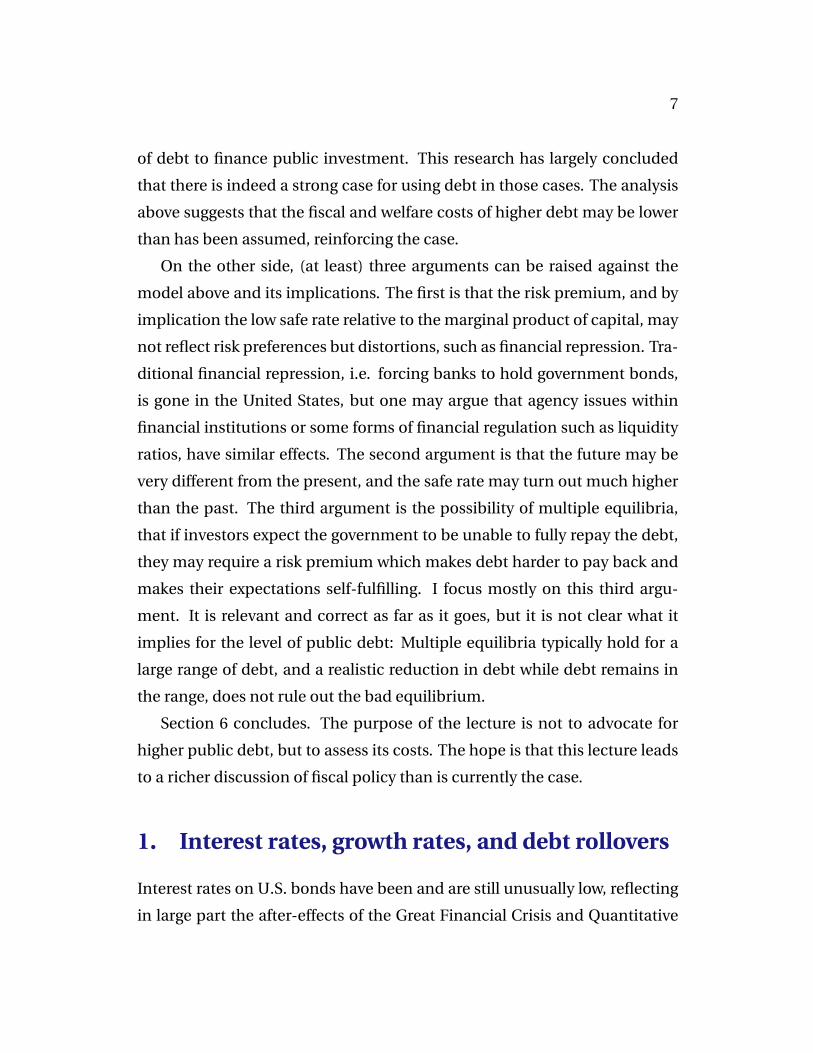
the post-1950 period.4 Figure 1 shows the evolution of nominal GDP growth

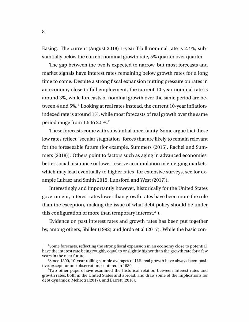
rate and the 1-year Treasury bill rate. Figure 2 shows the evolution of nomi-

nal GDP growth rate and the 10-year Treasury bond rate. Together, they have

two basic features:

Figure 1: Nominal growth rate and 1-year T-bill rate

‐4

‐2

0

2

4

6

8

10

12

14

16

Nominal growth rate and 1‐year T‐bill rate

1‐year T‐bill rate nominal growth rate

• On average, over the period, nominal interest rates have been lower

than nominal growth rates.5 The 1-year rate has averaged 4.7%, the 10-

year rate has averaged 5.6%, while nominal GDP growth has averaged

6.3%.6

4There is a striking difference not so much in the level but in the stochastic behavior ofrates pre- and post-1950, with a sharp decrease in volatility post-1950.

5Equivalently, if one uses the same deflator, real interest rates have been lower than thereal growth rate. Real interest rates are however often computed using CPI inflation ratherthan the GDP deflator.

6Using Shiller’s numbers for interest rates and historical BEA series for GDP, over thelonger period 1871 to 2018, the 1-year rate has averaged 4.6%, the 10-year rate 4.6% andnominal GDP growth 5.3%.

10

Figure 2: Nominal growth rate and 10-year bond rate

‐4

‐2

0

2

4

6

8

10

12

14

16Nominal growth rate and 10‐year bond rate

nominal 10‐year rate nominal growth rate

• Both the 1-year rate and the 10-year rate were consistently below the

growth rate until the disinflation of the early 1980s, Since then, both

nominal rates and nominal growth have declined, with rates declin-

ing faster than growth, even before the Great Financial Crisis. Over-

all, while nominal rates vary substantially from year to year, the 1-year

rate has been lower than the growth rate for all decades except for the

1980s. The 10-year rate has been lower than the growth rate for 4 out

of 7 decades.

Given that my focus is on the implications of the joint evolution of in-

terest rates and growth rates for debt dynamics, I must construct a series

for the relevant interest rate paid on public debt held by private investors.

I proceed in three steps, first taking into account the maturity composition

of the debt, second taking into account the tax payments on the interest re-

ceived by the holders of public debt, and third, taking into account Jensen’s

11

inequality. (Details of construction are given in appendix A.)

To take into account maturity, I use information on the average maturity

of the debt held by private investors (that is excluding public institutions

and the Fed.) This average maturity went down from 8 years and 4 months

in 1950 to 3 years and 4 months in 1974, with a mild increase since then to 5

years today.7 Given this series, I construct a maturity-weighted interest rate

as a weighted average of the 1-year and the 10-year rates using it = αt ∗ i1,t+(1− αt) ∗ i10,t with αt = (10− average maturity in years)/9.

Many, but not all, holders of government bonds pay taxes on the interest

paid, so the interest cost of debt is actually lower than the interest rate itself.

There is no direct measure of those taxes, and thus I proceed as follows.

I measure the tax rate of the marginal holder by looking at the difference

between the yield on AAA municipal bonds (which are exempt from Federal

taxes) and the yield on a corresponding maturity Treasury bond, for both 1-

year and 10-year bonds. Assuming that the marginal investor is indifferent

between holding the two, the implicit tax rate on 1-year treasuries is given

by τ1t = 1− imt1/i1t, and the implicit tax rate on 10-year Treasuries is given by

τ10t = 1− imt10/i10t.8 The tax rate on 1-year bonds peaks at about 50% in the

late 1970s (as inflation and nominal rates are high, leading to high effective

tax rates) down to close to zero until the Great Financial Crisis, and have

increased slightly since 2017. The tax rate on 10-year bonds follows a similar

pattern, down from about 40% in the early 1980s to close to zero, with a small

7Fed holdings used to be very small relative to total debt, and limited to short maturityT-bills. As a result of quantitative easing, they have become larger and skewed towards longmaturity bonds, implying a lower maturity of debt held by private investors than of totaldebt.

8This is an approximation. On the one hand, the average tax rate is likely to exceed thismarginal rate. On the other hand, to the extent that municipal bonds are also partially ex-empt from state taxes, the marginal tax rate may reflect in part the state tax rate in additionto the Federal tax rate.

12

increase since 2016. 9 Taking into account the maturity structure of the debt,

I then construct an average tax rate in the same way as I constructed the

interest rate above, by constructing τt = αt ∗ τ1,t + (1− αt) ∗ τ10,tNot all holders of Treasuries pay taxes however. Foreign holders, private

and public (such as central banks), Federal retirement programs and Fed

holdings are not subject to tax. The proportion of such holders has steadily

increased over time, reflecting the increase in emerging markets’ reserves (in

particular China’s), the growth of the Social Security Trust Fund, and more

recently, the increased holdings of the Fed, among other factors. From 15%

in 1950, it now accounts for 64% today.

Using the maturity adjusted interest rate from above, it, the implicit tax

rate, τt, and the proportion of holders likely subject to tax, βt, I construct an

“adjusted interest rate” series according to:

iadj,t = it(1− τt ∗ βt)

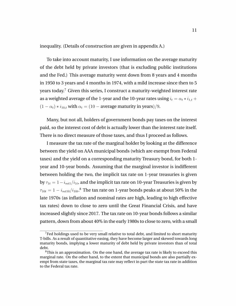
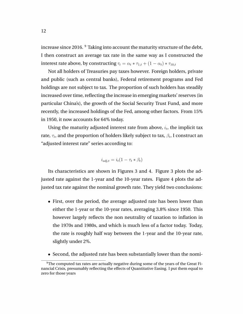
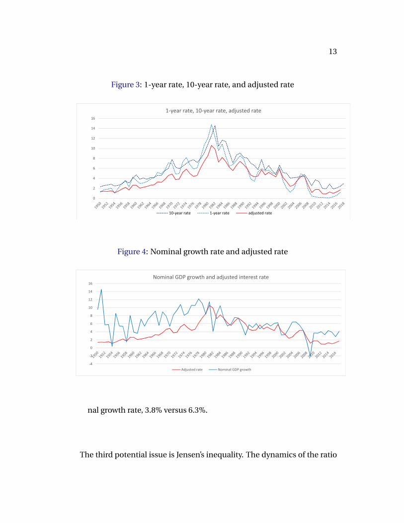
Its characteristics are shown in Figures 3 and 4. Figure 3 plots the ad-

justed rate against the 1-year and the 10-year rates. Figure 4 plots the ad-

justed tax rate against the nominal growth rate. They yield two conclusions:

• First, over the period, the average adjusted rate has been lower than

either the 1-year or the 10-year rates, averaging 3.8% since 1950. This

however largely reflects the non neutrality of taxation to inflation in

the 1970s and 1980s, and which is much less of a factor today. Today,

the rate is roughly half way between the 1-year and the 10-year rate,

slightly under 2%.

• Second, the adjusted rate has been substantially lower than the nomi-

9The computed tax rates are actually negative during some of the years of the Great Fi-nancial Crisis, presumably reflecting the effects of Quantitative Easing. I put them equal tozero for those years

13

Figure 3: 1-year rate, 10-year rate, and adjusted rate

0

2

4

6

8

10

12

14

16

1‐year rate, 10‐year rate, adjusted rate

10‐year rate 1‐year rate adjusted rate

Figure 4: Nominal growth rate and adjusted rate

‐4

‐2

0

2

4

6

8

10

12

14

16Nominal GDP growth and adjusted interest rate

Adjusted rate Nominal GDP growth

nal growth rate, 3.8% versus 6.3%.

The third potential issue is Jensen’s inequality. The dynamics of the ratio

14

of debt to GDP are given by:

dt =1 + radj,t1 + gt

dt−1 + xt

where dt is the ratio of debt to GDP (with both variables either in nominal

or in real terms if both are deflated by the same deflator), and xt is the ratio

of the primary deficit to GDP (again, with both variables either in nominal

or in real terms). The evolution of the ratio depends on the relevant product

of interest rates and growth rates (nominal or real) over time.

Given the focus on debt rollovers, that is the issuance of debt without a

later increase in taxes or reduction in spending, suppose we want to trace

debt dynamics under the assumption that xt remains equal to zero.10 Sup-

pose that ln[(1+ radj,t)/(1+ gt)] is distributed normally with mean µ and vari-

ance σ2. Then, the evolution of the ratio will depend not just on expµ but

on exp(µ + (1/2)σ2). We have seen that, historically, µ was between -1% and

-2%. The standard deviation of the log ratio over the same sample was equal

to 2.8%, implying a variance of 0.05%, thus too small to affect the conclu-

sions substantially. Jensen’s inequality is thus not an issue here.11

In short, if we assume that the future will be like the past (a big if admit-

tedly), debt rollovers—that is increases in debt without a change in the pri-

mary surplus—appear feasible. While the debt ratio may increase for some

time due to adverse shocks to growth or positive shocks to the interest rate,

it will eventually decrease over time. In other words, higher debt does not

imply a higher fiscal cost.

In this light, it is interesting to do the following counterfactual exercise.

Assume that the debt ratio in year t was what it actually was, but that the

10Given that we subtract taxes on interest from interest payments, the primary balancemust also be computed subtracting those tax payments.

11The conclusion is nearly the same if we do not assume log normality, but rather boot-strap from the actual distribution.

15

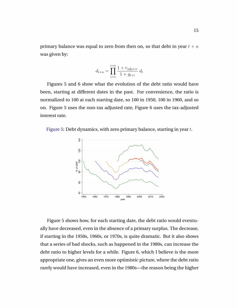
primary balance was equal to zero from then on, so that debt in year t + n

was given by:

dt+n =i=n∏i=1

1 + radj,t+i1 + gt+i

dt

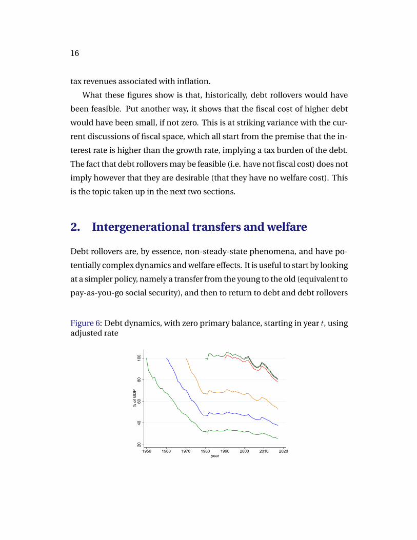
Figures 5 and 6 show what the evolution of the debt ratio would have

been, starting at different dates in the past. For convenience, the ratio is

normalized to 100 at each starting date, so 100 in 1950, 100 in 1960, and so

on. Figure 5 uses the non-tax adjusted rate, Figure 6 uses the tax-adjusted

interest rate.

Figure 5: Debt dynamics, with zero primary balance, starting in year t.

4060

8010

012

014

0%

of G

DP

1950 1960 1970 1980 1990 2000 2010 2020year

Figure 5 shows how, for each starting date, the debt ratio would eventu-

ally have decreased, even in the absence of a primary surplus. The decrease,

if starting in the 1950s, 1960s, or 1970s, is quite dramatic. But it also shows

that a series of bad shocks, such as happened in the 1980s, can increase the

debt ratio to higher levels for a while. Figure 6, which I believe is the more

appropriate one, gives an even more optimistic picture, where the debt ratio

rarely would have increased, even in the 1980s—the reason being the higher

16

tax revenues associated with inflation.

What these figures show is that, historically, debt rollovers would have

been feasible. Put another way, it shows that the fiscal cost of higher debt

would have been small, if not zero. This is at striking variance with the cur-

rent discussions of fiscal space, which all start from the premise that the in-

terest rate is higher than the growth rate, implying a tax burden of the debt.

The fact that debt rollovers may be feasible (i.e. have not fiscal cost) does not

imply however that they are desirable (that they have no welfare cost). This

is the topic taken up in the next two sections.

2. Intergenerational transfers and welfare

Debt rollovers are, by essence, non-steady-state phenomena, and have po-

tentially complex dynamics and welfare effects. It is useful to start by looking

at a simpler policy, namely a transfer from the young to the old (equivalent to

pay-as-you-go social security), and then to return to debt and debt rollovers

Figure 6: Debt dynamics, with zero primary balance, starting in year t, usingadjusted rate

2040

6080

100

% o

f GD

P

1950 1960 1970 1980 1990 2000 2010 2020year

17

in the next section.

The natural set-up to explore the issues is an overlapping generation model

under uncertainty. The overlapping generation structure implies a real effect

of intergenerational transfers or of debt, and the presence of uncertainty al-

lows to distinguish between the safe rate and the risky marginal product of

capital.

I proceed in two steps, first briefly reviewing the effects of a transfer un-

der certainty, following Diamond (1965), then extending it to uncertainty.

(Derivations are given in Appendix B)

Assume that the economy is populated by people who live for two peri-

ods, working in the first period, and consuming in both periods. Their utility

is given by:

U = (1− β)U(C1) + βU(C2)

where C1 and C2 are consumption in the first and the second period re-

spectively. (As I shall limit myself for the moment to looking at the effects

of the transfer on utility in steady state, there is no need for now for a time

index.) Their first and second period budget constraints are given by

C1 = W −K −D ;C2 = R K +D

,

where W is the wage, K is saving (equivalently, next period capital), D is

the transfer from young to old, and R is the rate of return on capital.

Production is given by a constant returns production function. I ignore

population growth and technological progress, so the growth rate is equal to

zero.

Y = F (K,N)

18

It is convenient to normalize labor to 1, so N = 1. Both factors are paid

their marginal product.

The first order condition for utility maximisation is given by:

(1− β) U ′(C1) = βR U ′(C2)

The effect of a small increase in the transfer D on utility is given by:

dU = [−(1− β)U ′(C1) + βU ′(C2)] dD + [(1− β)U ′(C1) dW + βKU ′(C2) dR]

The first term in brackets, call it dUa, represents the direct effect of the

transfer, the second term, call it dUb, the effect of the transfer through the

induced change in wages and rates of return.

Consider the first term, the effect of debt on utility given labor and capi-

tal prices. Using the first-order condition gives:

dUa = [β(−R U ′(C2) + U ′(C2))] dD = β(1−R)U ′(C2) dD (1)

So, if R < 1 (the case known as “dynamic inefficiency”), then, ignoring

the other term, a small increase in the transfer increases welfare. The expla-

nation is straightforward: If R < 1, the transfer gives a higher rate of return

to savers than does capital.

Take the second term, the effect of debt on utility through the changes in

W andR. An increase in debt decreases capital and thus decreases the wage

and increases the rate of return on capital. What is the effect on welfare?

Using the factor price frontier relation dW = −KdR, rewrite this second

term as:

19

dUb = −[(1− β)U ′(C1)− βU ′(C2)]K dR

Using the first order condition for utility maximization gives:

dUb = −[β(R− 1)U ′(C2)]K dR

Using the definition of the elasticity of substitution η ≡ (FKFN)/FKNF ,

the definition of the share of labor, α = FN/F , and the relation between

second derivatives of the production function, FNK = −KFKK , this second

term can be rewritten as:

dUb = [β(R− 1)U ′(C2)](1/η)αR dK (2)

Note the following three implications of equation (2):

• If R < 1, then a decrease in capital accumulation is good. This goes in

the same direction as the first effect.

• Putting the two effects together leads to the well known conclusion that

if the marginal product is less than the growth rate (which here is equal

to zero), an intergenerational transfer has a positive effect on welfare

in steady state.

• The strength of the second effect depends on the elasticity of substitu-

tion η. If for example η = ∞ so the production function is linear and

capital accumulation has no effect on either wages or rates of return to

capital, this second effect is equal to zero.

So far, I just replicated the analysis in Diamond.12 Now introduce uncer-

tainty in production, so the marginal product of capital is uncertain. If peo-

12Formally, Diamond looks at the effects of a change in debt rather than a transfer. But,under certainty and in steady state, the two are equivalent.

20

ple are risk averse, the average safe rate will be less than the average marginal

product of capital. The basic question becomes:

What is the relevant rate we should look at for welfare purposes? Put

loosely, is it the average marginal product of capital ER, or is it the average

safe rate ERf , or it is some other rate altogether?

The model is the same as before, except for the introduction of uncer-

tainty:

People born at time t have expected utility given by: (I now need time

subscripts as the steady state is stochastic):

U = (1− β)U(C1,t) + βEU(C2,t+1)

Their budget constraints are given by

C1t = Wt −Kt −D ;C2t+1 = Rt+1 Kt +D

Production is given by a constant returns production function

Yt = AtF (Kt−1, N)

whereN = 1 andAt is stochastic. (The capital at time t reflects the saving

of the young at time t− 1, thus the timing convention).

At time t, the first order condition for utility maximization is given by:

(1− β) U ′(C1,t) = βE[Rt+1 U′(C2,t+1)]

We can now define a shadow safe rate Rft+1, which must satisfy:

Rft+1E[U

′(C2,t+1] = E[Rt+1 U′(C2,t+1)]

21

Now consider a small increase in D on utility at time t:

dUt = [−(1−β)U ′(C1,t)+βEU′(C2,t+1)] dD+[(1−β)U ′(C1,t) dWt+βKtE(U

′(C2,t+1) dRt+1)]

As before, the first term in brackets, call it dUat, reflects the direct effect

of the transfer, the second term, call it dUbt, reflects the effect through the

change in wages and rates of return to capital.

Take the first term, the effect of debt on utility given prices. Using the

first order condition gives:

dUat = [−βE[Rt+1 U′(C2,t+1)] + βE[U ′(C2,t+1)]] dD

So:

dUat = β(1−Rft+1)EU

′(C2,t+1) dD (3)

So, to determine the sign effect of the transfer on welfare through this first

channel, the relevant rate is indeed the safe rate. In any period in whichRft+1

is less than one, the transfer is welfare improving.

The explanation is straightforward: The safe rate is, in effect, the risk

adjusted rate of return on capital.13 The intergenerational transfer gives a

higher rate of return to people than the risk adjusted rate of return on capi-

tal.

Take the second term, the effect on utility through prices:

13The low safe rate is sometimes explained as a result of a shift of the IS curve to theleft, requiring a lower rate to maintain output at potential (Summers 2018). It should beclear that this is another way of saying the same thing. The shift of the IS curve must bedue either to an increase in saving, or a decrease in investment due to either higher risk orhigher profitability.

22

dUbt = (1− β)U ′(C1,t) dWt + βKtEU′(C2,t+1) dRt+1

In general, this term will depend both on dKt−1 (which affects dWt) and

on dKt (which affects dRt+1). If we evaluate it at Kt = Kt−1 = K and dKt =

dKt+1 = dK, it can be rewritten, using the same steps as in the certainty case,

as:

dUbt = [β(1/η) α Rft+1 E[U

′(C2,t+1)]] (Rt − 1) dK (4)

Thus the relevant rate in assessing the sign of the welfare effect of the

transfer through this second term is the risky rate, the marginal product of

capital.

Putting the two sets of results together: If the safe rate is less than one,

and the risky rate is greater than one—the configuration which appears to

be relevant today—the two terms now work in opposite directions: The first

term implies that an increase in debt increases welfare. The second term

implies that an increase in debt instead decreases welfare. Both rates are

thus relevant.

To get a sense of relative magnitudes of the two effects, and therefore

which one is likely to dominate, the following approximation is useful: Eval-

uate the two terms at the average values of the safe and the risky rates, to

get:

dU/dD = [(1− ERf )− (1/η) α ERf (ER− 1)] βE[U ′(C2)](−dK/dD)

so that:

23

sign dU ≡ sign [(1− ERf )− (1/η)αERf (−dK/dD)(ER− 1)] (5)

where, from the accumulation equation, we have:

dK/dD = − 1

1− βα(1/η)ER

Note that, if the production is linear, and so η = ∞, the second term in

equation (6) is equal to zero, and the only rate that matters is ERf . Thus,

if ERf is less than one, a higher transfer increases welfare. As the elastic-

ity of substitution becomes smaller, the price effect becomes stronger, and,

eventually, the welfare effect changes sign and becomes negative.

In the Cobb-Douglas case, using the fact thatER ≈ (1−α)/(αβ), (the ap-

proximation comes from ignoring Jensen’s inequality) the equation reduces

to the simpler formula:

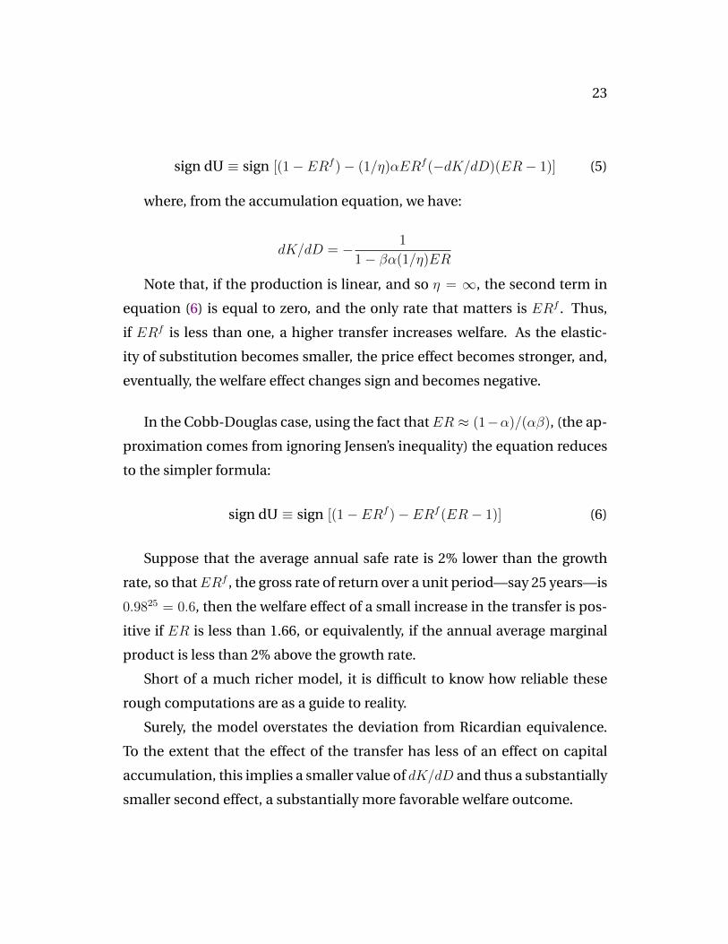
sign dU ≡ sign [(1− ERf )− ERf (ER− 1)] (6)

Suppose that the average annual safe rate is 2% lower than the growth

rate, so thatERf , the gross rate of return over a unit period—say 25 years—is

0.9825 = 0.6, then the welfare effect of a small increase in the transfer is pos-

itive if ER is less than 1.66, or equivalently, if the annual average marginal

product is less than 2% above the growth rate.

Short of a much richer model, it is difficult to know how reliable these

rough computations are as a guide to reality.

Surely, the model overstates the deviation from Ricardian equivalence.

To the extent that the effect of the transfer has less of an effect on capital

accumulation, this implies a smaller value of dK/dD and thus a substantially

smaller second effect, a substantially more favorable welfare outcome.

24

Surely also, the return to capital, given the price risk associated with hold-

ing shares, is substantially more risky than the return to labor, and this may

lead to a quantitatively different trade-off. Be that as it may, it suggests that

the welfare effects of a transfer may be not even be adverse, or, if adverse,

may not be very large.14

3. Simulations. Transfers, debt, and debt

rollovers

To get a more concrete picture, and turn to the effects of debt and debt

rollovers requires going to simulations.15 Within the structure of the model

above, I make the following specific assumptions: (Derivations are given in

Appendix C.)

I think of each of the two periods of life as equal to twenty five years.

Given the role of risk aversion in determining the gap between the average

safe and risky rates, I want to separate the elasticity of substitution across the

two periods of life and the degree of risk aversion. So I assume that utility has

an Epstein-Zin-Weil representation of the form (Epstein and Zin 2013), Weil

(1990)):

14Tentative: Note that the economy we are looking at is dynamically efficient in the senseof Zilcha (1991). Zilcha defined dynamic efficiency as the condition that there is no reallo-cation such that consumption of either the young or the old can be increased in at least onestate of nature and one period, and not decreased in any other; the motivation for the def-inition is that it makes the condition independent of preferences. He then showed that ina stationary economy, a necessary and sufficient condition for dynamic inefficiency is thatE lnR > 0. What the argument in the text has shown is that an intergenerational transfercan be welfare improving even if the Zilcha condition holds: As we saw, expected utility canincrease even if the average risky rate is large, so long as the safe rate is low enough. Thereallocation is such that consumption indeed decreases in some states, yet expected utilityis increased.

15One can make some progress analytically, and we did characterize the behavior of debtat the margin (that is when taking the no-debt prices as given) in Blanchard and Weil (1990),for a number of different utility and production functions. We only focused on debt dynam-ics however, and not on the normative implications.

25

(1− β) lnC1t + β1

1− γlnE(C1−γ

2t+1)

The log-log specification implies that the intertemporal elasticity of sub-

stitution is equal to 1. The coefficient of relative risk aversion is given by γ.

As the strength of the second effect above depends on the elasticity of

substitution between capital and labor, I assume a CES production function,

with multiplicative uncertainty:

Yt = At (bKρt−1 + (1− b)Nρ)1/ρ = At(bK

ρt−1 + (1− b))1/ρ

whereAt is white noise and is distributed log normally, with lnAt ∼ N (µ;σ2)

and ρ = (η−1)/η, where η is the elasticity of substitution. When η =∞, ρ = 1

and the production function is linear.

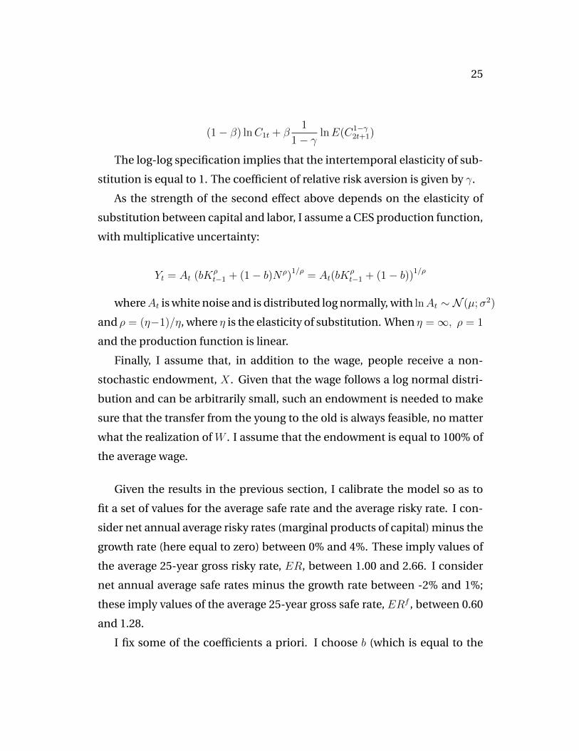
Finally, I assume that, in addition to the wage, people receive a non-

stochastic endowment, X. Given that the wage follows a log normal distri-

bution and can be arbitrarily small, such an endowment is needed to make

sure that the transfer from the young to the old is always feasible, no matter

what the realization of W . I assume that the endowment is equal to 100% of

the average wage.

Given the results in the previous section, I calibrate the model so as to

fit a set of values for the average safe rate and the average risky rate. I con-

sider net annual average risky rates (marginal products of capital) minus the

growth rate (here equal to zero) between 0% and 4%. These imply values of

the average 25-year gross risky rate, ER, between 1.00 and 2.66. I consider

net annual average safe rates minus the growth rate between -2% and 1%;

these imply values of the average 25-year gross safe rate, ERf , between 0.60

and 1.28.

I fix some of the coefficients a priori. I choose b (which is equal to the

26

capital share in the Cobb-Douglas case)to 1/3. For reasons explained below,

I choose the annual value of σa to be a high 4% a year, which implies a value

of σ of√25 ∗ 4% = 0.20.

Because the strength of the second effect above depends on the elastic-

ity of substitution, I consider two different values of η, η = ∞ which corre-

sponds to the linear production function case, and in which the price effects

of lower capital accumulation is equal to zero, and η = 1, the Cobb-Douglas

case, and the case which is generally seen as a good description of the pro-

duction function in the medium run.

The central parameters are, on the one hand, β and µ, and on the other,

γ.

The parameters β and µ determine (together with σ, which plays a mi-

nor role) the average level of capital accumulation and the average marginal

product of capital, the average risky rate. In general, both parameters matter.

In the linear production case however, the marginal product of capital is in-

dependent of the level of capital, and thus depends only on µ; thus, I choose

µ to fit the average value of the marginal product. In the Cobb-Douglas case,

the marginal product of capital is instead independent of µ and depends

only on β; thus I choose β to fit the average value of the marginal product of

capital.

The parameter γ determines, together with σ the spread between the

risky rate and the safe rate. In the absence of transfers, the following rela-

tion holds between the two rates:

lnRft+1 − lnERt+1 = −γσ2

This relation implies however that the model suffers from a strong case

of the equity premium puzzle (see for example Kocherlakota (1996)). If we

think of σ as the standard deviation of TFP growth, and assume that, in the

27

data, TFP growth is a random walk (with drift), this implies an annual value

of σa of about 2%, thus a value of σ over the 25-year period of 10%, and thus

a value of σ2 of 1%. Thus, if we think of the annual risk premium as, say,

5%, which implies a value of the right hand side of about 1.22, this implies

a value of γ, the coefficient of relative risk aversion of 122, which is clearly

implausible. One of the reasons why the model fails so badly is the symme-

try in the degree of uncertainty facing labor and capital, and the absence of

price risk associated with holding shares (as capital fully depreciates within

the 25-year period). If we take instead σ to reflect the standard deviation of

yearly rates of stock returns, say 15% a year (its historical mean), and assume

stock returns to be uncorrelated over time, then σ over the 25-year period is

equal to 75%, implying values of γ around 2.5. There is no satisfactory way to

deal with the issue within the model, so as an uneasy compromise, I choose

σ = 20%. Given σ, γ is determined for each pair of average risky and safe

rates.16

I then consider the effects on welfare of an intergenerational transfer.

The basic results are summarized in the four figures below.

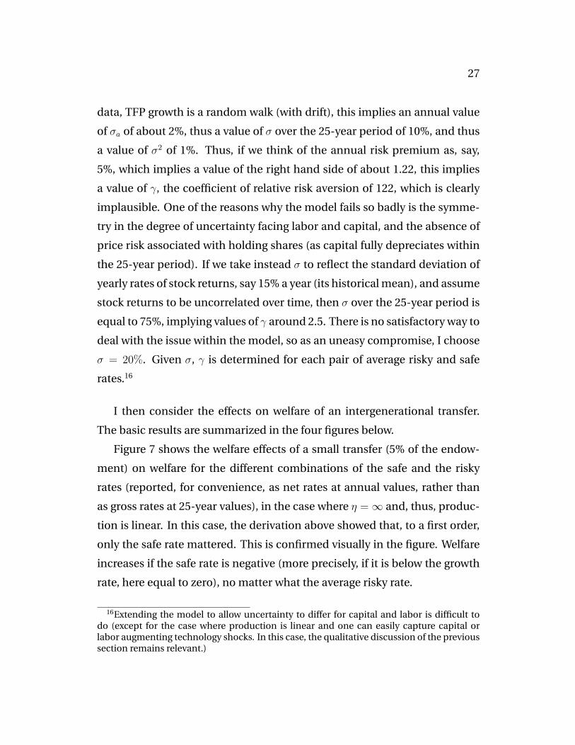
Figure 7 shows the welfare effects of a small transfer (5% of the endow-

ment) on welfare for the different combinations of the safe and the risky

rates (reported, for convenience, as net rates at annual values, rather than

as gross rates at 25-year values), in the case where η =∞ and, thus, produc-

tion is linear. In this case, the derivation above showed that, to a first order,

only the safe rate mattered. This is confirmed visually in the figure. Welfare

increases if the safe rate is negative (more precisely, if it is below the growth

rate, here equal to zero), no matter what the average risky rate.

16Extending the model to allow uncertainty to differ for capital and labor is difficult todo (except for the case where production is linear and one can easily capture capital orlabor augmenting technology shocks. In this case, the qualitative discussion of the previoussection remains relevant.)

28

Figure 7: Welfare effects of higher debt 5% (linear production function)

-1

-0.5

0

0.5

1

1.5

2

4 3.5 3 2.5 2 1.5 1 -2 -1.50.5 -1 -0.50 0 0.5 1

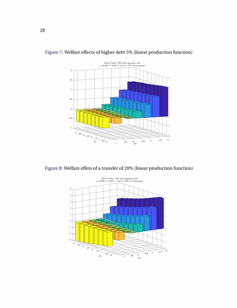
Figure 8: Welfare effets of a transfer of 20% (linear production function)

-3

-2

-1

0

1

2

3

4

4

5

3.53

2.52 -2 1.5 -1.51 -1 -0.50.5 0 0 0.5 1

29

Figure 8 looks at a larger transfer (20% of the endowment), again in the

linear production case. For a givenRf , a largerER leads to a smaller welfare

increase if welfare increases, and to a larger welfare decrease if welfare de-

creases. The reason is as follows: As the size of the transfer increases, second

period income becomes less risky, so the risk premium decreases, increas-

ing Rf for given average R. In the limit, a transfer which led people to save

nothing in capital would eliminate uncertainty about second period income,

and thus would lead to Rf = ER. The larger R, the faster Rf increases with

a large transfer; for ER high enough , and for D large enough, Rf becomes

larger than one, and the transfer becomes welfare decreasing.

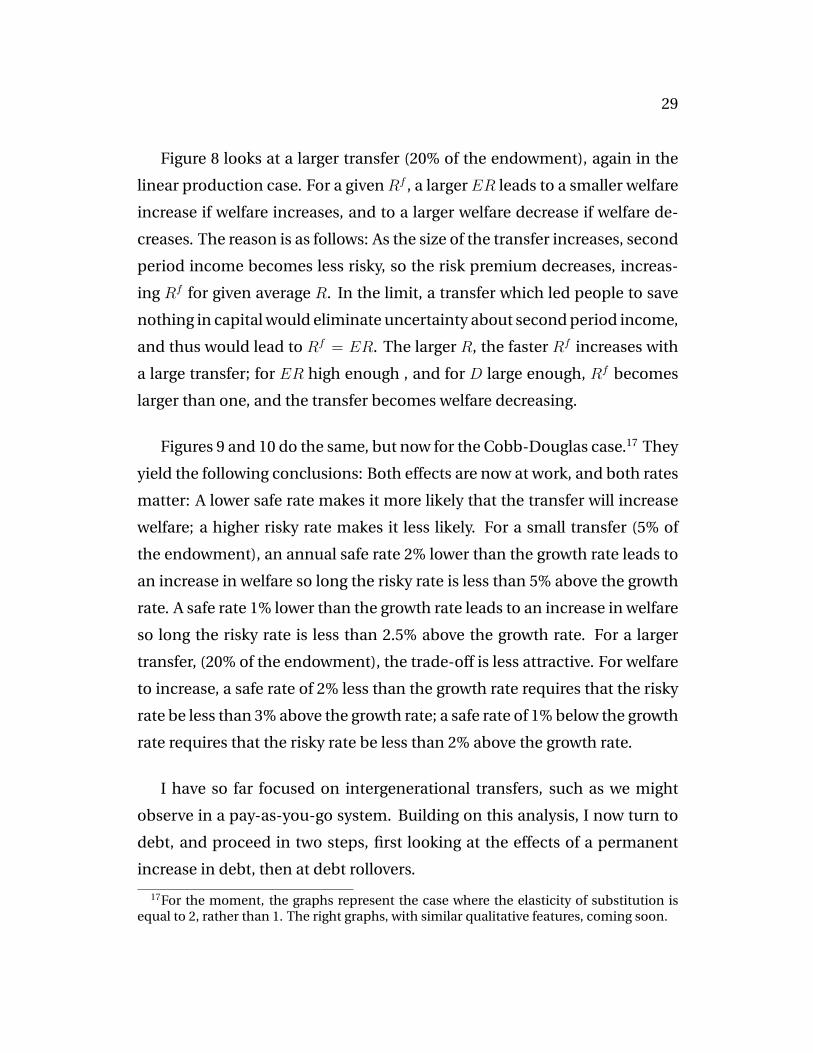
Figures 9 and 10 do the same, but now for the Cobb-Douglas case.17 They

yield the following conclusions: Both effects are now at work, and both rates

matter: A lower safe rate makes it more likely that the transfer will increase

welfare; a higher risky rate makes it less likely. For a small transfer (5% of

the endowment), an annual safe rate 2% lower than the growth rate leads to

an increase in welfare so long the risky rate is less than 5% above the growth

rate. A safe rate 1% lower than the growth rate leads to an increase in welfare

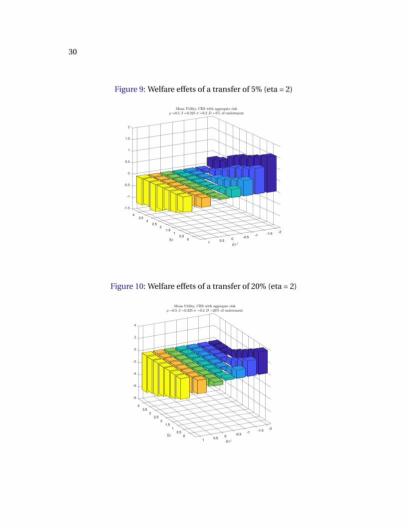
so long the risky rate is less than 2.5% above the growth rate. For a larger

transfer, (20% of the endowment), the trade-off is less attractive. For welfare

to increase, a safe rate of 2% less than the growth rate requires that the risky

rate be less than 3% above the growth rate; a safe rate of 1% below the growth

rate requires that the risky rate be less than 2% above the growth rate.

I have so far focused on intergenerational transfers, such as we might

observe in a pay-as-you-go system. Building on this analysis, I now turn to

debt, and proceed in two steps, first looking at the effects of a permanent

increase in debt, then at debt rollovers.

17For the moment, the graphs represent the case where the elasticity of substitution isequal to 2, rather than 1. The right graphs, with similar qualitative features, coming soon.

30

Figure 9: Welfare effets of a transfer of 5% (eta = 2)

-1.5

-1

-0.5

0

0.5

1

4

1.5

2

3.53

2.52

1.5 -2 1 -1.5-1 0.5 -0.50 0 0.5 1

Figure 10: Welfare effets of a transfer of 20% (eta = 2)

-8

-6

-4

-2

4

0

2

4

3.53

2.52

1.51 -2 -1.50.5 -1 -0.50 0 0.5 1

31

Suppose the government increases the level of debt and maintains it at

this higher level forever. Depending on the value of the safe rate every pe-

riod, this may require either issuing new debt when Rft < 1 and distribut-

ing the proceeds as benefits, or retiring debt, when Rft > 1 and financing

it through taxes. Following Diamond, assume that benefits and taxes are

paid to, or levied on, the young. In this case, the budget constraints faced by

somebody born at time t are given:

C1t = (Wt +X + (1−Rft )D)− (Kt +D) = Wt +X −Kt −DRf

t

C2t+1 = Rt+1Kt +DRft+1

So, a constant level of debt can be thought of as an intergenerational

transfer, with a small difference relative to the case developed earlier. The

difference is that a generation born at t makes a net transfer of DRft when

young, and receives, when old, a net transfer of DRft + 1, as opposed to the

one-for-one transfer studied earlier. Under certainty, in steady state, Rf is

constant and the two are equivalent. Under uncertainty, the variation about

the terms of the intertemporal transfer imply a smaller increase in welfare

than in the transfer case. Otherwise, the conclusions are very similar.

A debt rollover is somewhat different. As the government issues debt D0,

and never pays it back, there are neither taxes nor subsidies after the initial

issuance and associated transfer. The budget constraints faced by somebody

born at time t are given by:

C1t = (Wt +X − (Kt +Dt)

32

C2t+1 = Rt+1Kt +DtRft+1

And debt follows:

Dt = Rft Dt−1

First, consider sustainability. Even if debt decreases in expected value

over time, a debt rollover, i.e. the issuance of debt paying Rft , may fail with

positive probability. A sequence of realizations of Rft > 1 may increase debt

to the level where Rf becomes larger than one and remains so, leading to a

debt explosion. At some point, an adjustment will have to take place, either

through default, or through an increase in taxes. The probability of such a

sequence over a long but finite period of time is however likely to be small,

if Rf starts far below 1.18

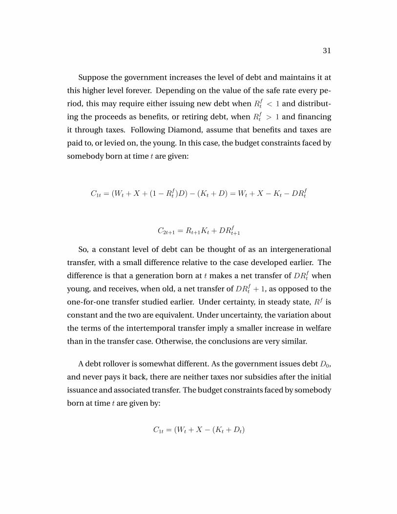
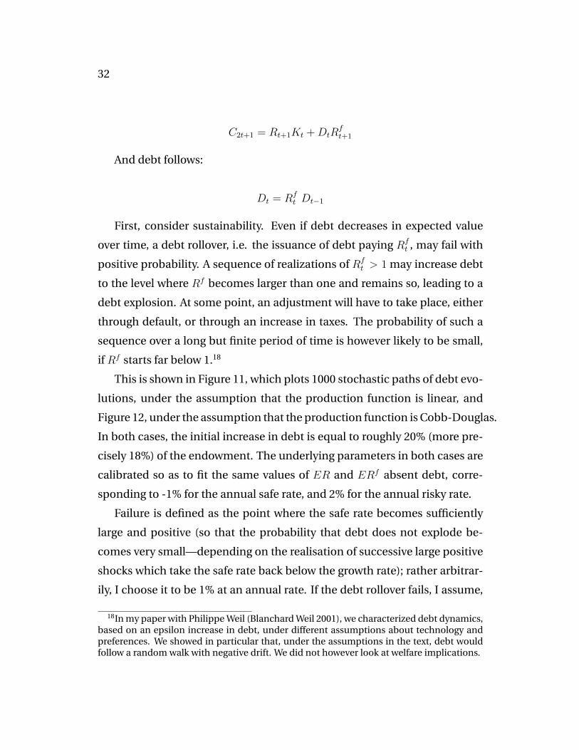
This is shown in Figure 11, which plots 1000 stochastic paths of debt evo-

lutions, under the assumption that the production function is linear, and

Figure 12, under the assumption that the production function is Cobb-Douglas.

In both cases, the initial increase in debt is equal to roughly 20% (more pre-

cisely 18%) of the endowment. The underlying parameters in both cases are

calibrated so as to fit the same values of ER and ERf absent debt, corre-

sponding to -1% for the annual safe rate, and 2% for the annual risky rate.

Failure is defined as the point where the safe rate becomes sufficiently

large and positive (so that the probability that debt does not explode be-

comes very small—depending on the realisation of successive large positive

shocks which take the safe rate back below the growth rate); rather arbitrar-

ily, I choose it to be 1% at an annual rate. If the debt rollover fails, I assume,

18In my paper with Philippe Weil (Blanchard Weil 2001), we characterized debt dynamics,based on an epsilon increase in debt, under different assumptions about technology andpreferences. We showed in particular that, under the assumptions in the text, debt wouldfollow a random walk with negative drift. We did not however look at welfare implications.

33

again arbitrarily and too strongly, that all debt is paid back through a tax on

the young.19 This exaggerates the effect of failure on the young in that pe-

riod, but is simplest to capture.

In the linear case, the higher debt and lower capital accumulation have

no effect on the risky rate, and a limited effect on the safe rate, and all paths

show declining debt. Four periods out (100 years), all of them have lower

debt than at the start.

Figure 11: Linear production function. Debt evolutions under a debt rolloverD0= 18% of endowment

en

-�rn

,,......_

<l)l:f:.... '----'

� en

�

Debt Share of Savings, Linear OLG With Uncertainty ER=2% ERf=-1% initdebt =16.875%

20 -----,f--------------'--------------'-------------'---------------+-

18

16

14

12

10

8

6-----,f-------------�------------r---------------r---------------+-

0 25 50 Time (year)

75 100

In the Cobb-Douglas case, with the same values of ER and ERf absent

debt, bad shocks, which lead to higher debt and lower capital accumulation,

lead to increases in the risky rate, and by implication, larger increases in the

safe rate. The result is that, for the same shocks, 5% of paths fail over the

first four periods. Are these Ponzi gambles—as Ball, Elmendorf and Mankiw

have called them—worth it at least from a fiscal viewpoint? If the probability

of failure is low enough, they might well be.

19The alternative would be a tax on the old. This however would make public debt riskythroughout, and lead to a much harder problem to solve.

34

Figure 12: Cobb-Douglas production function. Debt evolutions under a debtrollover D0= 18% of endowment

Debt Share of Savings, CB OLG With Uncertainty ER=2% ERf=-1% initdebt =16.875%

35 -----,f--------------'--------------'-------------'---------------+-

en b.() � -�rn

4-. o-

30

25

<l) i:f: 20 .... '----'

� en

..., ..0 <l)

� 15

10

5-----,f-------------�------------r--------------r---------------+-

0 25 50 Time (year)

75 100

Second, consider to welfare effects: Relative to a pay-as-you-go scheme,

debt rollovers are much less attractive. Remember the two effects of an inter-

generational transfer. The first effect comes from the fact that people receive

a rate of return of 1 on the transfer, a rate which is higher than Rft . In a debt

rollover, they receive a rate of return of only Rft < 1. At the margin, they are

indifferent to holding debt or capital. There is still an inframarginal effect, a

consumer surplus (taking the form of a less risky portfolio), but the positive

effect on welfare is smaller than in the straight transfer scheme. The sec-

ond effect, due to the change in wages and rate of return on capital, is still

present, so the net effect on welfare, while less persistent as debt decreases

over time, is more likely to be negative.

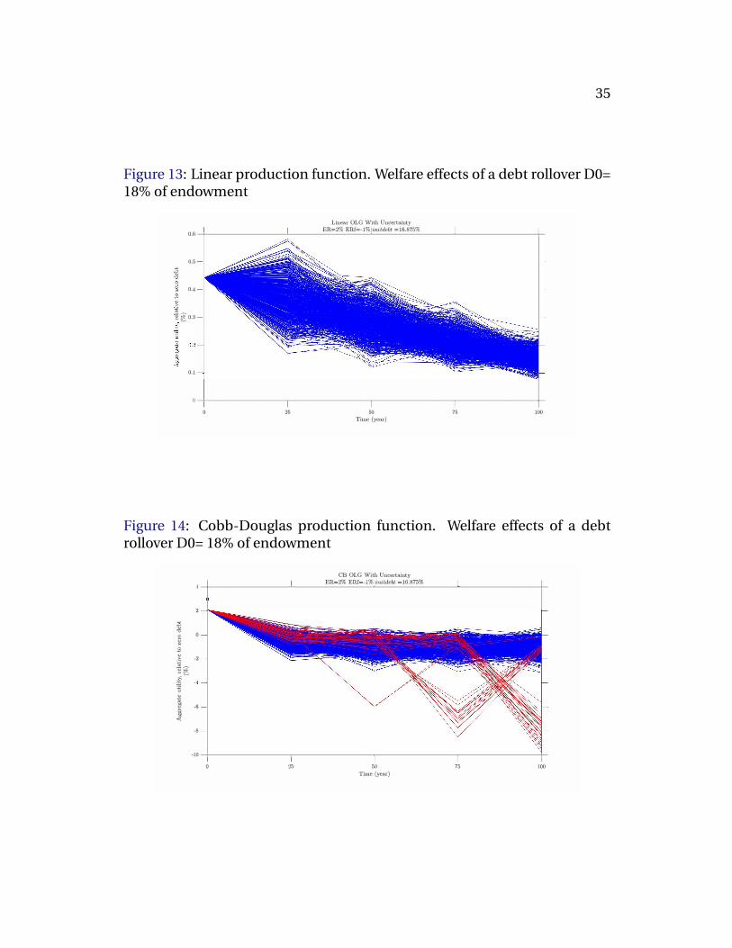
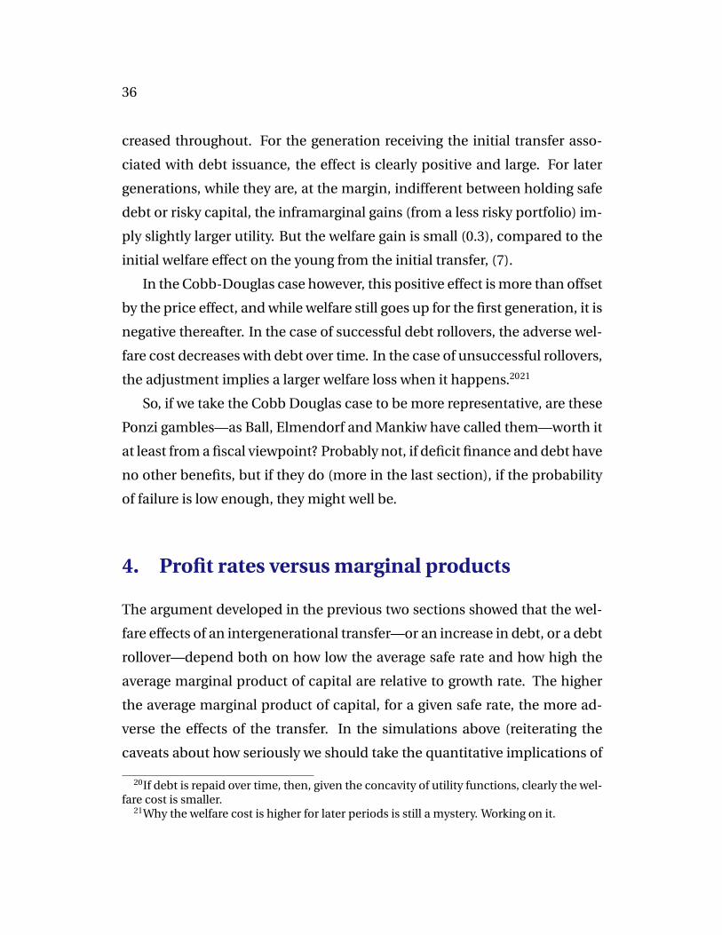
This is shown in Figures 13 and 14, which show the average welfare effects

of successful and unsuccessful debt rollovers, for the linear and the Cobb-

Douglas case.

In the linear case, debt rollovers typically do not fail and welfare is in-

35

Figure 13: Linear production function. Welfare effects of a debt rollover D0=18% of endowment

Linear OLG With Uncertainty ER=2% ERf=-1% initdebt =16.875%

0.6 -t-------------�------------�------------�------------+--

0.5

0.4

� �0.3

0.1

0-t-------------�------------�------------�------------+--

0 25 50 Time (year)

75 100

Figure 14: Cobb-Douglas production function. Welfare effects of a debtrollover D0= 18% of endowment

...., i; "::)

0 '"' (1) " 0 ...., (1)

,;:;...., o:l -

al � ...

;,:.;...., �....,;:I

(1) ...., o:l b.O (1) '"' b.O b.O

�

CB OLG With Uncertainty ER=2% ERf=-1% initdebt =16.875%

4-----,f--------------'--------------'-------------'---------------+-

2

0

-2

-4

-6

-8

-10 -----,f--------------r--------------r--------------r---------------+-

0 25 50 Time (year)

75 100

36

creased throughout. For the generation receiving the initial transfer asso-

ciated with debt issuance, the effect is clearly positive and large. For later

generations, while they are, at the margin, indifferent between holding safe

debt or risky capital, the inframarginal gains (from a less risky portfolio) im-

ply slightly larger utility. But the welfare gain is small (0.3), compared to the

initial welfare effect on the young from the initial transfer, (7).

In the Cobb-Douglas case however, this positive effect is more than offset

by the price effect, and while welfare still goes up for the first generation, it is

negative thereafter. In the case of successful debt rollovers, the adverse wel-

fare cost decreases with debt over time. In the case of unsuccessful rollovers,

the adjustment implies a larger welfare loss when it happens.2021

So, if we take the Cobb Douglas case to be more representative, are these

Ponzi gambles—as Ball, Elmendorf and Mankiw have called them—worth it

at least from a fiscal viewpoint? Probably not, if deficit finance and debt have

no other benefits, but if they do (more in the last section), if the probability

of failure is low enough, they might well be.

4. Profit rates versus marginal products

The argument developed in the previous two sections showed that the wel-

fare effects of an intergenerational transfer—or an increase in debt, or a debt

rollover—depend both on how low the average safe rate and how high the

average marginal product of capital are relative to growth rate. The higher

the average marginal product of capital, for a given safe rate, the more ad-

verse the effects of the transfer. In the simulations above (reiterating the

caveats about how seriously we should take the quantitative implications of

20If debt is repaid over time, then, given the concavity of utility functions, clearly the wel-fare cost is smaller.

21Why the welfare cost is higher for later periods is still a mystery. Working on it.

37

that model), the welfare effects of an average marginal product far above the

growth rate typically dominated the effects of an average safe slightly below

the growth rate, implying a negative effect of the transfer (or of debt) on wel-

fare.

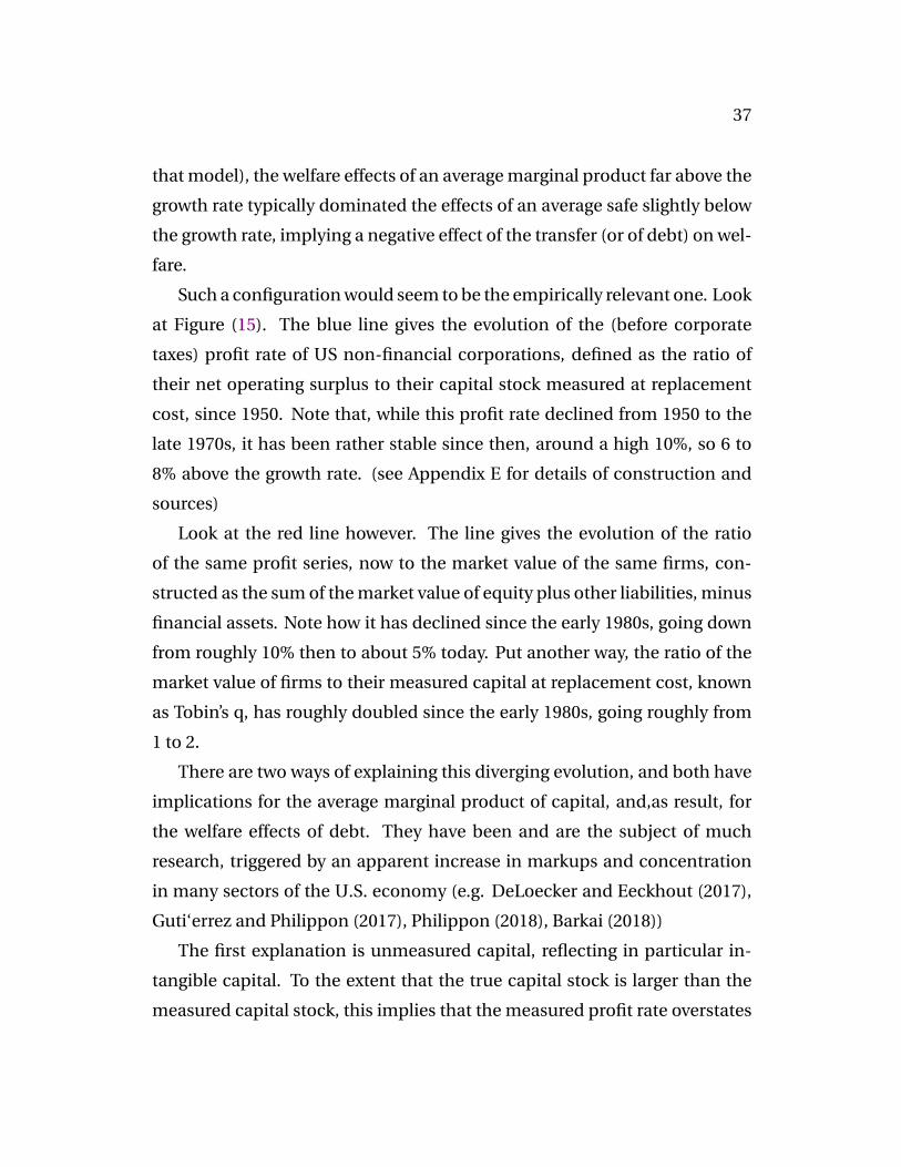
Such a configuration would seem to be the empirically relevant one. Look

at Figure (15). The blue line gives the evolution of the (before corporate

taxes) profit rate of US non-financial corporations, defined as the ratio of

their net operating surplus to their capital stock measured at replacement

cost, since 1950. Note that, while this profit rate declined from 1950 to the

late 1970s, it has been rather stable since then, around a high 10%, so 6 to

8% above the growth rate. (see Appendix E for details of construction and

sources)

Look at the red line however. The line gives the evolution of the ratio

of the same profit series, now to the market value of the same firms, con-

structed as the sum of the market value of equity plus other liabilities, minus

financial assets. Note how it has declined since the early 1980s, going down

from roughly 10% then to about 5% today. Put another way, the ratio of the

market value of firms to their measured capital at replacement cost, known

as Tobin’s q, has roughly doubled since the early 1980s, going roughly from

1 to 2.

There are two ways of explaining this diverging evolution, and both have

implications for the average marginal product of capital, and,as result, for

the welfare effects of debt. They have been and are the subject of much

research, triggered by an apparent increase in markups and concentration

in many sectors of the U.S. economy (e.g. DeLoecker and Eeckhout (2017),

Guti‘errez and Philippon (2017), Philippon (2018), Barkai (2018))

The first explanation is unmeasured capital, reflecting in particular in-

tangible capital. To the extent that the true capital stock is larger than the

measured capital stock, this implies that the measured profit rate overstates

38

0

2

4

6

8

10

12

14

16

18

1950 1953 1956 1959 1962 1965 1968 1971 1974 1977 1980 1983 1986 1989 1992 1995 1998 2001 2004 2007 2010 2013 2016

Profit over capital at replacement cost Profit over market value

Figure 15: Profit over replacement cost, Profit over market value since 1950

the true profit rate, and by implication overstates the marginal product of

capital. A number of researchers have explored this hypothesis, and their

conclusion is that, even if the adjustment already made by the Bureau of

Economic Analysis is insufficient, intangible capital would have to be im-

plausibly large to reconcile the evolution of the two series: Measured intan-

gible capital as a share of capital has increased from 6% in 1980 to 15% to-

day. Suppose it had in fact increased by 25%. This would only lead to a 10%

increase in measured capital, far from enough to explain the divergent evo-

lutions of the two series.22

The second explanation is increasing rents, reflecting in particular the

increasing relevance of increasing returns to scale and increased concentra-

tion. If, so the profit rate reflects not only the marginal product of capital,

but also rents. The market value of firms reflects not only the value of capital

but also the present value of rents. If we take all of the increase in the ratio of

the market value of firms to capital at replacement cost to reflect an increase

in rents, the doubling of the ratio implies that rents account for roughly half

22Further discussion can be found in Barkai 2018.

39

of profit.23

As on each of the issues raised in this lecture, many caveats are in order,

and they are being taken on by current research. Movements in Tobin’s q,

the ratio of market value to capital, are often difficult to explain.24 Yet, the

evidence is fairly consistent with a decrease in the average marginal product

of capital, and by implication, a smaller welfare cost of debt.

5. A broader view. Arguments and

counterarguments

So far, I have considered the effects of debt when debt was used to finance

intergenerational transfers in a full employment economy. This was in order

to focus on the basic mechanisms at work. But it clearly did not do justice

to the potential benefits of debt finance, nor does it address other potential

costs of debt left out of the model. The purpose of this last section is to dis-

cuss potential benefits and potential costs. As this touches on many aspects

of the economy and many lines of research, it is informal, more in the way

of remarks and research leads than definitive answers about optimal debt

policy.

Start with potential benefits. The standard argument for deficit finance

in a country like the United States is its potential role in increasing demand

and reducing the output gap when the economy is in recession. The Great

23A rough arithmetic exercise: Suppose V = qK + PDV (R), where V is the value offirms, q is the shadow price of capital, R is rents. The shadow price is in turn given byq = PDV (MPK)/K. Look at the medium run where adjustment costs have worked out,so q = 1. Then V/K − 1 = PDV (R)/PDV (MPK). If V/K doubles from 1 to 2, then thisimplies that PDV (R) = PDV (MPK), so rents account for half of total profits.

24In particular, what makes me slightly uncomfortable with the argument is the behaviorof Tobin’s q from 1950 to 1980, which roughly halved. Was it because of decreasing rentsthen?

40

Financial crisis, and the role of both the initial fiscal expansion and the later

turn to fiscal austerity, has led to a resurgence of research on the topic. Re-

search has been active on three fronts:

The first has revisited the size of fiscal multipliers. Larger multipliers im-

ply a smaller increase in debt for a given fiscal expansion. Looking at the

Great Financial crisis, two arguments have been made that multipliers were

higher during that time. First, lower ability to borrow by both households

and firms implied a stronger effect of current income as opposed to future

income on spending, and thus a stronger multiplier. Second, at the effective

lower bound, monetary authorities did not feel they should increase interest

rates in the response to the fiscal expansion. 25

The second front, explored by DeLong and Summers (2012) has revisited

the effect of fiscal expansions on output and debt in the presence of hys-

teresis. They have shown that even a small hysteretic effect of a recession

on later output might lead a fiscal expansion to actually reduce rather than

increase debt in the long run, with the effect being stronger, the stronger the

multipliers and the lower the safe interest rate.26 Note that this is a differ-

ent argument from the argument developed in this paper: The proposition

is that a fiscal expansion may not increase debt, while the argument of the

paper is that an increase in debt may have small fiscal and welfare costs. The

two arguments are clearly complementary however.

The third front has been that public investment has been too low, often

being the main victim of fiscal consolidation, and that the marginal prod-

uct of public capital is high. The relevant point here is that what should be

compared is the risk adjusted rate of return on public investment to the risk

25For a review of the empirical evidence up to 2010 see Ramey (2011). For more recentcontributions, see, for example, Mertens (2018) on tax multipliers, and the debate betweenAuerbach and Gorodnichenko (2012) and Ramey and Zubairy (2018.)

26I examined the evidence for or against hysteresis in Blanchard (2017). I concluded thatthe evidence was not strong enough to move priors, for or against, very much.

41

adjusted rate of return on private capital, i.e. the safe rate.

Let me however concentrate on potential costs of debt, and some coun-

terarguments to the earlier conclusions that debt may have low fiscal or wel-

fare costs. I can think of three main counterarguments:

The first is that the safe rate may be artificially low, so the welfare implica-

tions above may not hold. It is indeed generally agreed that US government

bonds benefit not only from low risk, but also from a liquidity discount, lead-

ing to a lower safe rate than would otherwise be the case. The issue however

is whether this discount reflect technology and preferences, or distortions in

the financial system. If they reflect liquidity services valued by households

and firms, then the logic of the earlier model applies: The safe rate is now

the liquidity-adjusted and risk-adjusted equivalent of the marginal product

of capital and is thus what must be compared to the growth rate. If how-

ever, the liquidity discount reflects distortions, for example financial repres-

sion forcing financial institutions to hold government bonds, then indeed

the safe rate is no longer the appropriate rate to compare to growth. It may

be welfare improving in this case to reduce financial repression even if this

leads to a higher safe rate, and a higher cost of public debt. Straight financial

repression is no longer relevant for the United States, but various agency is-

sues internal to financial institutions as well as financial regulations such as

liquidity requirements, may have some of the same effects.

The second counterargument is that the future may be different from

the past, and that, despite the long historical record, safe interest rates may

become consistently higher than the growth rate. This may be because to-

tal factor productivity growth remains very low, and combined with aging,

leads to an even lower growth rate than currently forecast.27 It may be be-

27In infinite horizon models a la Ramsey, the Euler equation leads to a tight relation be-tween growth rates and interest rates, so that if growth comes down, so does the interest

42

cause some of the factors underlying low rates fade over time. Or it may be

because public debt increases to the point where the equilibrium safe rate

actually exceeds the growth rate. In the formal model above, a high enough

level of debt, and the associated decline in capital accumulation, may well

lead to an increase in the safe rate above the growth rate, leading to positive

fiscal costs and higher welfare costs. Indeed, the trajectory of deficits under

current fiscal plans is indeed worrisome. Estimates by Sheiner (2018) for ex-

ample suggest, despite the assumption that the safe rate remains below the

growth rate, we may see an increase in the ratio of debt to GDP of close to

60% of GDP between now and 2043. If so, using a standard back of the enve-

lope number that an increase in debt of 1% of GDP increases the safe rate by

2-3 basis points, this would lead to an increase in the safe rate of 1.2 to 1.8%,

enough to reverse the inequality.

History may indeed not be a reliable guide to the future. As the debates

on secular stagnation and the level of the long run Wicksellian rate (the safe

rate consistent with unemployment remaining at the natural rate) indicate,

the future is indeed uncertain,and this uncertainty should be taken into ac-

count. The evidence on indexed bonds suggests however two reasons to

be relatively optimistic. The first is that, to the extent that the U.S. govern-

ment can finance itself through inflation-indexed bonds, it can lock in a rate

of 1% over the next 30 years, a rate far below even pessimistic forecasts of

growth over the same period. The second is that investors seem to give a

small probability to a major increase in rates. Looking at 10-year inflation-

indexed bonds, and using realized volatility as a proxy for implied volatility,

suggests that the market puts the probability that the rate will be higher than

200 bp in five years, at around 12%.28 Thus, debt may indeed be more costly

rate. In the data, the relation between growth rates and interest rates is much weaker.28The daily standard deviation is around 3bp, implying a 5-year standard deviation of√1250 ∗ 2 − 3bp = 70-105 bp. This implies that the probability that the rate, which today is

100bp, is larger than 200bp is about 15%.

43

in the future. The welfare results above however are continuous, and for rea-

sonably small positive differences between the interest rate and the growth

rate, the welfare effects may remain small. The basic intuition remains the

same: The safe rate is the risk adjusted rate of return on capital. If it is low,

lower capital accumulation may not have major adverse welfare effects.

The third counterargument relies on the existence of multiple equilibria

and may be the more difficult to counter.29 Suppose that the model above

is right, and that, indeed, investors believe debt to be safe and are willing

to hold it at the safe rate. In this case, the fiscal cost of debt may indeed be

zero, and the welfare cost small. If however, investors believe that debt is

risky and ask for a risk premium to compensate for that risk, debt payments

will be larger, and debt will indeed be risky, and investors’ expectations may

be self fulfilling.

The mechanics of such fiscal multiple equilibria were first characterized

by Calvo (1988), Giavazzi and Pagano (1990), and more recently by, among

others, Lorenzoni and Werning (2018)). In this case, over a wide range of

debt, there may be two equilibria, with the good one being the one where

the safe rate is low, and the bad one characterized by high risk, a high risk

premium on public debt, and a high interest rate.30

The question is what practical implications this has for debt levels. The

first question is whether there is a debt level sufficiently low as to elimi-

nate the multiplicity. If we ignore strategic default, there must be some low

enough debt level such that the debt is effectively safe and there is only one

29It feels less relevant for the United States than for other countries, emerging marketcountries in particular. But, as debt to GDP ratios increase, it may not be irrelevant.

30Under either formal or informal dynamics, the good equilibrium is stable, while the badequilibrium is unstable. However, what may happen in this case, is that the economy movesto a position worse than the bad equilibrium, with interest rates and risk premia increasingtowards infinity. A straightforward extension of the model above, showing the nature of thetwo equilibria, is sketched in Appendix F.

44

equilibrium. Suppose investors worry about risk and increase the required

rate. As the required rate goes to infinity, the state will default. But suppose

that, even if it defaults, debt is low enough that, while it cannot pay the stated

rate, it can pay the safe rate. This in turn implies that investors, if they are

rational, should not and will not worry about risk. This however raises two

issues. First, it may be difficult to assess what such a safe level of debt is: it

is likely to depend on the nature of the government, on its ability to increase

and maintain a primary surplus. Second, the safe level of debt may be very

low, much lower than current levels of debt in the United States and in Eu-

rope. If multiple equilibria are present at, say 100% of GDP, they are likely

to still be present at 90% as well; going however from 100% of GDP to 90%

requires a major fiscal contraction and potentially a large economic con-

traction, if, for example, it cannot be fully offset by expansionary monetary

policy. As Giavazzi and Pagano, and Lorenzoni and Werning have shown,

other dimensions of debt and fiscal policy, such as the maturity of debt or

the aggressiveness of the fiscal rule, are likely to be more important than the

level of debt itself, and allow to preserve the good equilibrium.

6. Conclusions

The lecture has looked at the fiscal and welfare costs of higher debt in an

economy where the safe interest rate is less than the growth rate. It has ar-

gued that this is a relevant empirical configuration, and indeed has been the

norm in the United States over the recent and more distant past. It has ar-

gued that both the fiscal and welfare costs of debt may then be small, smaller

than is generally taken as given in current policy discussions. It has consid-

ered a number of counterarguments, which are indeed valid, and may imply

larger fiscal and welfare costs. The purpose of this lecture is most definitely

not to argue for higher debt per se, but to allow for a richer discussion of debt

45

policy than is currently the case.

46

References

[1] Alan Auerbach and Yury Gorodnichenko. Measuring the output re-

sponses to fiscal policy. American Economic Journal: Economic Policy,

4(2):1–27, 2012.

[2] Laurence Ball, Douglas Emendorf, and N. Gregory Mankiw. The deficit

gamble. Journal of Money, Credit and Banking, 30(4):699–720, Novem-

ber 1998.

[3] Simcha Barkai. Declining labor and capital shares. 2018. ms, LSE.

[4] Philip Barrett. Interest-growth differentials and debt limits in advanced

economies. April 2018. IMF Working Paper.

[5] Olivier Blanchard. Should we reject the natural rate hypothesis? Journal

of Economic Perspectives, 32(1):97–120, Winter 2018.

[6] Olivier Blanchard and Philippe Weil. Dynamic efficiency, the riskless

rate, and debt ponzi games under uncertainty. Advances in Macroeco-

nomics, pages 1–23, November 2001.

[7] Guillermo Calvo. Servicing the public debt: The role of expectations.

American Economic Review, 78(4):647–661, September 1988.

[8] Jan De Loecker and Jan Eeckhout. The rise of market power and the

macroeconomic implications. August 2017. ms, Princeton.

[9] Brad deLong and Lawrence Summers. Fiscal policy in a depressed

economy. Brookings Papers on Economic Activity, 2012:233–297, Spring

2012.

[10] Peter Diamond. National debt in a neoclassical growth model. Ameri-

can Economic Review, 55(5-1):1126–1150, December 1965.

47

[11] Larry Epstein and Stanley Zin. Substitution, risk aversion, and the tem-

poral behavior of consumption and asset returns. a theoretical frame-

work. Handbook of the Fundamentals of Financial Decision Making,

pages 207–239, 2013.

[12] Francesco Giavazzi and Marco Pagano. Confidence crisis and pub-

lic debt management. 1990. Capital Markets and Debt Manage-

ment. Mario Draghi and Rudiger Dornbusch (eds.) Cambridge Univer-

sity Press.

[13] German Gutierrez and Thomas Philippon. Declining competition and

investment in the u.s. November 2017. ms, New York University.

[14] Oscar Jorda, Katharina Knoll, Dmitry Kuvshinov, Moritz Schularicl, and

Alan Taylor. The rate of return on everything, 1870-2015. December

2017. Federal Reserve Bank of San Francisco Working Paper 2017-25.

[15] Narayana Kocherlakota. The equity premium: It’s still a puzzle. Journal

of Economic Literature, 34(1):42–71, March 1996.

[16] Guido Lorenzoni and Ivan Werning. Slow moving debt crises. July 2018.

ms, MIT.

[17] Rachel Lukasz and Thomas Smith2015. Secular drivers of the global

real interest rate. 1(2), December 2015. Staff Working Paper, Bank of

England.

[18] Kurt Lunsford and Kenneth West. Some evidence on secular drivers of

us safe real rates. 2017. Federal Reserve Bank of Cleveland Working

Paper 17-23.

[19] Neil Mehrotra. Implications of low productivity growth for debt sus-

tainability. 1(2), November 2017. manuscript, Brown University.

48

[20] Karel Mertens. The near term growth impact of the tax cuts and jobs

act. March 2018. FRB Dallas.

[21] Thomas Philippon. A primer on concentration, investment, and

growth. August 2017. Prepared for the Jackson Hole Economic Policy

Symposium.

[22] Lukasz Rachel and Lawrence Summers. The equilibrium real interest

rate in advanced economies: The role of of government policies and

current account imbalances. July 2018. ms, Harvard and LSE.

[23] Valerie Ramey. Can government purchases stimulate the economy?

Journal of Economic Literature, 49(3):673–685, September 2011.

[24] Valerie Ramey and Sarah Zubairy. Government spending multipliers in

good times and in bad: Evidence from u.s. historical data. 2018. ms,

forthcoming, JPE.

[25] Louise Sheiner. The effects of low productivity growth on fiscal sustain-

ability. May 2018. ms, Peterson Institute for International Economics.

[26] Robert Shiller. Market Volatility. MIT Press, 1992.

[27] Lawrence Summers. Demand side secular stagnation. American Eco-

nomic Review Papers and Proceedings, 105:60–65, May 2001.

[28] Philippe Weil. Nonexpected utility in macroeconomics. Quarterly Jour-

nal of Economics, 105(1):29–42, February 1990.

[29] Itzhak Zilcha. Characterizing efficiency in stochastic overlapping gen-

erations models. Journal of Economic Theory, 55:1–16, 1991.