
Psychology 454: Latent Variable Modeling Week 4: … · Example data sets Thurstone 9 variable...
75
Example data sets Thurstone 9 variable problem Confirmatory fits Holzinger 14 cognitive variables Using lavaan References Psychology 454: Latent Variable Modeling Week 4: Latent models of real data William Revelle Department of Psychology Northwestern University Evanston, Illinois USA October, 2015 1 / 74
Transcript of Psychology 454: Latent Variable Modeling Week 4: … · Example data sets Thurstone 9 variable...

Example data sets Thurstone 9 variable problem Confirmatory fits Holzinger 14 cognitive variables Using lavaan References
Psychology 454: Latent Variable ModelingWeek 4: Latent models of real data
William Revelle
Department of PsychologyNorthwestern UniversityEvanston, Illinois USA
October, 2015
1 / 74

Example data sets Thurstone 9 variable problem Confirmatory fits Holzinger 14 cognitive variables Using lavaan References
Outline
Example data setsGetting real data – either from examples or your ownFirst, a brief diversion with simulation
Thurstone 9 variable problemFactor extraction: how many and what algorithmVarious Rotations or Transformations
Confirmatory fitsUsing semBifactor modelsConfirmatory Bifactor model
Holzinger 14 cognitive variables
Using lavaanTraditional analyses of the Holzinger Swineford data setSEM analysis of Holzinger Swineford data set
2 / 74
Example data sets Thurstone 9 variable problem Confirmatory fits Holzinger 14 cognitive variables Using lavaan References
Real data rather than simulated
1. Prior examples were all artificial data sets.• These have the advantage that we know truth.• They have the disadvantage that they don’t give us experience
with real data.
2. Some classic data sets are available in psych, lavaan and sem.
3. Using the data function to see what is available.• data(package="psych")
4. Eventually, you need to try your own data.
3 / 74

Example data sets Thurstone 9 variable problem Confirmatory fits Holzinger 14 cognitive variables Using lavaan References
Some of the psych data setsdata(package="psych")
Bechtoldt Seven data sets showing a bifactor solution.Bechtoldt.1 Seven data sets showing a bifactor solution.Bechtoldt.2 Seven data sets showing a bifactor solution.Chen (Schmid) 12 variables created by Schmid and Leiman to show the
Schmid-Leiman TransformationDwyer 8 cognitive variables used by Dwyer for an example.Gorsuch Example data set from Gorsuch (1997) for an example factor
extension.Harman.5 5 socio-economic variables from Harman (1967)Harman.8 Correlations of eight physical variables (from Harman, 1966)Harman.Burt (Harman) Two data sets from Harman (1967). 9 cognitive variables from
Holzinger and 8 emotional variables from BurtHarman.Holzinger (Harman) Two data sets from Harman (1967). 9 cognitive variables from
Holzinger and 8 emotional variables from BurtHolzinger Seven data sets showing a bifactor solution.Holzinger.9 Seven data sets showing a bifactor solution.Reise Seven data sets showing a bifactor solution.Schmid 12 variables created by Schmid and Leiman to show the
Schmid-Leiman TransformationThurstone Seven data sets showing a bifactor solution.Thurstone.33 Seven data sets showing a bifactor solution.Tucker 9 Cognitive variables discussed by Tucker and Lewis (1973)West (Schmid) 12 variables created by Schmid and Leiman to show the
Schmid-Leiman Transformationall.income (income) US family income from US census 2008bfi 25 Personality items representing 5 factorsblot Bonds Logical Operations Test - BLOTbock.table (bock) Bock and Liberman (1970) data set of 1000 observations of
the LSAT
4 / 74

Example data sets Thurstone 9 variable problem Confirmatory fits Holzinger 14 cognitive variables Using lavaan References
More of the psych data setsburt 11 emotional variables from Burt (1915)cities Distances between 11 US citiescity.location (cities) Distances between 11 US citiescubits Galtons example of the relationship between height and
cubit or forearm lengthcushny A data set from Cushny and Peebles (1905) on the effect of
three drugs on hours of sleep, used by Student (1908)epi.bfi 13 personality scales from the Eysenck Personality Inventory
and Big 5 inventoryflat (affect) Two data sets of affect and arousal scores as a function of
personality and movie conditionsgalton Galton Mid parent child height dataheights A data.frame of the Galton (1888) height and cubit data set.income US family income from US census 2008iqitems 16 multiple choice IQ itemslsat6 (bock) Bock and Liberman (1970) data set of 1000 observations of
the LSATlsat7 (bock) Bock and Liberman (1970) data set of 1000 observations of
the LSATmaps (affect) Two data sets of affect and arousal scores as a function of
personality and movie conditionsmsq 75 mood items from the Motivational State Questionnaire for
3896 participantsneo NEO correlation matrix from the NEO_PI_R manualpeas Galtons Peassat.act 3 Measures of ability: SATV, SATQ, ACTschmid.leiman (Schmid) 12 variables created by Schmid and Leiman to show the
Schmid-Leiman Transformationveg (vegetables) Paired comparison of preferences for 9 vegetableswithinBetween An example of the distinction between within group and
between group correlations5 / 74

Example data sets Thurstone 9 variable problem Confirmatory fits Holzinger 14 cognitive variables Using lavaan References
Data sets in sem and lavaan
data(package='sem')data(package ='lavaan')
Data sets in package 'sem':
Bollen Bollen''s Data on Industrialization and Political DemocracyCNES Variables from the 1997 Canadian National Election StudyKlein Klein''s Data on the U. S. Economy'Kmenta Partly Artificial Data on the U. S. Economy
Data sets in package 'lavaan':
Demo.growth Demo dataset for a illustrating a linear growth model.HolzingerSwineford1939 Holzinger and Swineford Dataset (9 Variables)PoliticalDemocracy Industrialization And Political Democracy Dataset
6 / 74

Example data sets Thurstone 9 variable problem Confirmatory fits Holzinger 14 cognitive variables Using lavaan References
Also can read in from clipboard, web, from hard drive and import
• To read from clipboard: read.clipboard()• read.clipboard(header = TRUE, ...) #assumes headers and
tab or space delimited• read.clipboard.csv(header=TRUE,sep=’,’,...) #assumes
headers and comma delimited• read.clipboard.tab(header=TRUE,sep=’�’,...) #assumes
headers and tab delimited• read.clipboard.lower(diag=TRUE,names=FALSE,...) #read in
a matrix given the lower off diagonal• read.clipboard.upper(diag=TRUE,names=FALSE,...)• read.clipboard.fwf(header=FALSE,widths=rep(1,10),...) #read
in data using a fixed format width (see read.fwf forinstructions)
• To read from a file• fn <- file.choose() #this opens the system directory – navigate
it to your file• my.data <- read.table(fn)
7 / 74

Example data sets Thurstone 9 variable problem Confirmatory fits Holzinger 14 cognitive variables Using lavaan References
More on getting your data
#specify the name and address of the remote filedatafilename <- "http://personality-project.org/r/datasets/maps.mixx.epi.bfi.data"#datafilename <- Desktop/epi.big5.txt #read from local directory or# datafilename <- file.choose() # use the OS to find the file#in all casesperson.data <- read.table(datafilename,header=TRUE) #read the data file
#Alternatively, to read in a comma delimited file:#person.data <- read.table(datafilename,header=TRUE,sep=",")
names(person.data) #list the names of the variables
library(foreign) #allows you to read SPSS files e.g.,datafilename <- "/Users/bill/Library/Favorites/R.tutorial/datasets/finkel.sav" #local fileeli.data <- read.spss(datafilename, use.value.labels=TRUE, to.data.frame=TRUE)
8 / 74

Example data sets Thurstone 9 variable problem Confirmatory fits Holzinger 14 cognitive variables Using lavaan References
Use the bifactor examples
The study of latent variable models in general and sem in particularis the combination of measurement models with structural models.The bifactor examples are useful to understand issues in reliabilityand estimating measurement models.data(Thurstone)data(Thurstone.33)data(Holzinger)data(Holzinger.9)data(Bechtoldt)data(Bechtoldt.1)data(Bechtoldt.2)data(Reise)data(Chen)data(West)
Two more data sets with similar structures are found in the Harman data set.
Bechtoldt.1: 17 x 17 correlation matrix of ability tests, N = 212.Bechtoldt.2: 17 x 17 correlation matrix of ability tests, N = 213.Holzinger: 14 x 14 correlation matrix of ability tests, N = 355Holzinger.9: 9 x 9 correlation matrix of ability tests, N = 145Reise: 16 x 16 correlation matrix of health satisfaction items. N = 35,000Thurstone: 9 x 9 correlation matrix of ability tests, N = 213Thurstone.33: Another 9 x 9 correlation matrix of ability items, N=4175
9 / 74

Example data sets Thurstone 9 variable problem Confirmatory fits Holzinger 14 cognitive variables Using lavaan References
Simulate a bifactor model using sim.structure
First, make up a bifactor model and then simulate it. We use thesim.structure function with a specified factor loadings matrix.
R code
f <- matrix(c(.8,.75,.7,.65,.6,.65,.7,.8,.9,.5,.6,.5,rep(0,9),.6,.5,.4, rep(0,9),.6,.5,.4),ncol=4)
f
[,1] [,2] [,3] [,4][1,] 0.80 0.5 0.0 0.0[2,] 0.75 0.6 0.0 0.0[3,] 0.70 0.5 0.0 0.0[4,] 0.65 0.0 0.6 0.0[5,] 0.60 0.0 0.5 0.0[6,] 0.65 0.0 0.4 0.0[7,] 0.70 0.0 0.0 0.6[8,] 0.80 0.0 0.0 0.5[9,] 0.90 0.0 0.0 0.4
10 / 74

Example data sets Thurstone 9 variable problem Confirmatory fits Holzinger 14 cognitive variables Using lavaan References
Simulate the dataR code
R <- sim.structure(f,n=500)R
Call: sim.structure(fx = f, n = 500)$model (Population correlation matrix)
V1 V2 V3 V4 V5 V6 V7 V8 V9V1 1.00 0.90 0.81 0.52 0.48 0.52 0.56 0.64 0.72V2 0.90 1.00 0.82 0.49 0.45 0.49 0.52 0.60 0.68V3 0.81 0.82 1.00 0.45 0.42 0.45 0.49 0.56 0.63V4 0.52 0.49 0.45 1.00 0.69 0.66 0.45 0.52 0.59V5 0.48 0.45 0.42 0.69 1.00 0.59 0.42 0.48 0.54V6 0.52 0.49 0.45 0.66 0.59 1.00 0.45 0.52 0.59V7 0.56 0.52 0.49 0.45 0.42 0.45 1.00 0.86 0.87V8 0.64 0.60 0.56 0.52 0.48 0.52 0.86 1.00 0.92V9 0.72 0.68 0.63 0.59 0.54 0.59 0.87 0.92 1.00$reliability (population reliability)[1] 0.89 0.92 0.74 0.78 0.61 0.58 0.85 0.89 0.97$r (Sample correlation matrix for sample size = 500 )
V1 V2 V3 V4 V5 V6 V7 V8 V9V1 1.00 0.91 0.83 0.52 0.47 0.54 0.61 0.66 0.74V2 0.91 1.00 0.85 0.49 0.44 0.51 0.57 0.62 0.70V3 0.83 0.85 1.00 0.45 0.40 0.45 0.54 0.59 0.66V4 0.52 0.49 0.45 1.00 0.73 0.65 0.48 0.55 0.60V5 0.47 0.44 0.40 0.73 1.00 0.64 0.50 0.54 0.58V6 0.54 0.51 0.45 0.65 0.64 1.00 0.48 0.54 0.61V7 0.61 0.57 0.54 0.48 0.50 0.48 1.00 0.87 0.88V8 0.66 0.62 0.59 0.55 0.54 0.54 0.87 1.00 0.93V9 0.74 0.70 0.66 0.60 0.58 0.61 0.88 0.93 1.00
11 / 74
Example data sets Thurstone 9 variable problem Confirmatory fits Holzinger 14 cognitive variables Using lavaan References
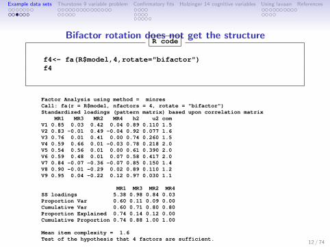
Bifactor rotation does not get the structureR code
f4<- fa(R$model,4,rotate="bifactor")f4
Factor Analysis using method = minresCall: fa(r = R$model, nfactors = 4, rotate = "bifactor")Standardized loadings (pattern matrix) based upon correlation matrix
MR1 MR3 MR2 MR4 h2 u2 comV1 0.85 0.03 0.42 0.04 0.89 0.110 1.5V2 0.83 -0.01 0.49 -0.04 0.92 0.077 1.6V3 0.76 0.01 0.41 0.00 0.74 0.260 1.5V4 0.59 0.66 0.01 -0.03 0.78 0.218 2.0V5 0.54 0.56 0.01 0.00 0.61 0.390 2.0V6 0.59 0.48 0.01 0.07 0.58 0.417 2.0V7 0.84 -0.07 -0.36 -0.07 0.85 0.150 1.4V8 0.90 -0.01 -0.29 0.02 0.89 0.110 1.2V9 0.95 0.04 -0.22 0.12 0.97 0.030 1.1
MR1 MR3 MR2 MR4SS loadings 5.38 0.98 0.84 0.03Proportion Var 0.60 0.11 0.09 0.00Cumulative Var 0.60 0.71 0.80 0.80Proportion Explained 0.74 0.14 0.12 0.00Cumulative Proportion 0.74 0.88 1.00 1.00
Mean item complexity = 1.6Test of the hypothesis that 4 factors are sufficient.
The degrees of freedom for the null model are 36 and the objective function was 8.96The degrees of freedom for the model are 6 and the objective function was 0
The root mean square of the residuals (RMSR) is 0The df corrected root mean square of the residuals is 0
Fit based upon off diagonal values = 1Measures of factor score adequacy
MR1 MR3 MR2 MR4Correlation of scores with factors 0.99 0.87 0.94 0.49Multiple R square of scores with factors 0.98 0.76 0.89 0.24Minimum correlation of possible factor scores 0.96 0.52 0.78 -0.53
12 / 74
Example data sets Thurstone 9 variable problem Confirmatory fits Holzinger 14 cognitive variables Using lavaan References
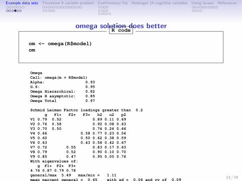
omega solution does betterR code
om <- omega(R$model)om
OmegaCall: omega(m = R$model)Alpha: 0.93G.6: 0.95Omega Hierarchical: 0.82Omega H asymptotic: 0.85Omega Total 0.97
Schmid Leiman Factor loadings greater than 0.2g F1* F2* F3* h2 u2 p2
V1 0.79 0.52 0.89 0.11 0.69V2 0.76 0.58 0.92 0.08 0.63V3 0.70 0.50 0.74 0.26 0.66V4 0.66 0.58 0.77 0.23 0.56V5 0.60 0.50 0.62 0.38 0.59V6 0.63 0.43 0.58 0.42 0.67V7 0.72 0.55 0.83 0.17 0.63V8 0.79 0.52 0.90 0.10 0.70V9 0.85 0.47 0.95 0.05 0.76With eigenvalues of:
g F1* F2* F3*4.76 0.87 0.79 0.78general/max 5.49 max/min = 1.11mean percent general = 0.65 with sd = 0.06 and cv of 0.09Explained Common Variance of the general factor = 0.66The degrees of freedom are 12 and the fit is 0.01The root mean square of the residuals is 0The df corrected root mean square of the residuals is 0Compare this with the adequacy of just a general factor and no group factorsThe degrees of freedom for just the general factor are 27 and the fit is 3.12The root mean square of the residuals is 0.13The df corrected root mean square of the residuals is 0.16
13 / 74

Example data sets Thurstone 9 variable problem Confirmatory fits Holzinger 14 cognitive variables Using lavaan References
lavaan gets the right answer (if we help)R code
library(lavaan)bi.mod <- 'g =~ V1 + V2 + V3 + V4 + V5 + V6 + V7 + V8 + V9
F1 =~ V1 + V2 + V3F2 =~ V4 + V5 + V6F3 =~ V7 + V8 + V9'
bi.cfa <- cfa(model=bi.mod,sample.cov=R$model,sample.nobs=500,orthogonal=TRUE,std.lv=TRUE)
summary(bi.cfa)
lavaan (0.5-19) converged normally after 42 iterations
Number of observations 500
Estimator MLMinimum Function Test Statistic 0.000Degrees of freedom 18P-value (Chi-square) 1.000
Parameter Estimates:
Information ExpectedStandard Errors Standard
14 / 74

Example data sets Thurstone 9 variable problem Confirmatory fits Holzinger 14 cognitive variables Using lavaan References
lavaan loadings are correct
But, we had to specify that we wanted an orthogonal solutionR code
bi.cfa <- cfa(model=bi.mod,sample.cov=R$model,sample.nobs=500,orthogonal=TRUE,std.lv=TRUE)
Latent Variables:Estimate Std.Err Z-value P(>|z|)
g =~V1 0.799 0.040 19.957 0.000V2 0.749 0.041 18.229 0.000V3 0.699 0.042 16.623 0.000V4 0.649 0.042 15.345 0.000V5 0.599 0.043 13.887 0.000V6 0.649 0.042 15.345 0.000V7 0.699 0.044 15.750 0.000V8 0.799 0.042 19.059 0.000V9 0.899 0.039 23.086 0.000
F1 =~V1 0.499 0.034 14.709 0.000V2 0.599 0.033 18.408 0.000V3 0.499 0.037 13.386 0.000
F2 =~V4 0.599 0.048 12.532 0.000V5 0.499 0.047 10.586 0.000V6 0.400 0.044 9.130 0.000
F3 =~V7 0.599 0.039 15.337 0.000V8 0.499 0.041 12.228 0.000V9 0.400 0.040 9.976 0.000
15 / 74

Example data sets Thurstone 9 variable problem Confirmatory fits Holzinger 14 cognitive variables Using lavaan References
Thurstone correlation matrix
> colnames(Thurstone) <- abbreviate(rownames(Thurstone),6)> Thurstone
Sntncs Vcblry Snt.Cm Frst.L 4.Lt.W Suffxs Lttr.S Pedgrs Lttr.GSentences 1.000 0.828 0.776 0.439 0.432 0.447 0.447 0.541 0.380Vocabulary 0.828 1.000 0.779 0.493 0.464 0.489 0.432 0.537 0.358Sent.Completion 0.776 0.779 1.000 0.460 0.425 0.443 0.401 0.534 0.359First.Letters 0.439 0.493 0.460 1.000 0.674 0.590 0.381 0.350 0.4244.Letter.Words 0.432 0.464 0.425 0.674 1.000 0.541 0.402 0.367 0.446Suffixes 0.447 0.489 0.443 0.590 0.541 1.000 0.288 0.320 0.325Letter.Series 0.447 0.432 0.401 0.381 0.402 0.288 1.000 0.555 0.598Pedigrees 0.541 0.537 0.534 0.350 0.367 0.320 0.555 1.000 0.452Letter.Group 0.380 0.358 0.359 0.424 0.446 0.325 0.598 0.452 1.000
The Thurstone 9 variable problem is taken from Bechtoldt (1961)who took data from Thurstone & Thurstone (1941) and split itinto two samples of 212 and 213. McDonald (1999) in turn tookthe 17 variables and chose 9 that show a clear bifactor structure.This example is used in the sem pacakge as well as PROC CALISin SAS.
16 / 74

Example data sets Thurstone 9 variable problem Confirmatory fits Holzinger 14 cognitive variables Using lavaan References
Better yet, use lowerMat
R code
lowerMat(Thurstone)
Sntnc Vcblr Snt.C Frs.L 4.L.W Sffxs Ltt.S Pdgrs Ltt.GSentences 1.00Vocabulary 0.83 1.00Sent.Completion 0.78 0.78 1.00First.Letters 0.44 0.49 0.46 1.004.Letter.Words 0.43 0.46 0.42 0.67 1.00Suffixes 0.45 0.49 0.44 0.59 0.54 1.00Letter.Series 0.45 0.43 0.40 0.38 0.40 0.29 1.00Pedigrees 0.54 0.54 0.53 0.35 0.37 0.32 0.56 1.00Letter.Group 0.38 0.36 0.36 0.42 0.45 0.32 0.60 0.45 1.00
17 / 74

Example data sets Thurstone 9 variable problem Confirmatory fits Holzinger 14 cognitive variables Using lavaan References
Or, if you like APA style tables in Latex use cor2latex
R code
cor2latex(Thurstone, font.size='tiny')
Table: cor2latex
A correlation table from the psych package in R.Variable Sntnc Vcblr Snt.C Frs.L 4.L.W Sffxs Ltt.S Pdgrs Ltt.GSentences 1.00Vocabulary 0.83 1.00Sent.Completion 0.78 0.78 1.00First.Letters 0.44 0.49 0.46 1.004.Letter.Words 0.43 0.46 0.42 0.67 1.00Suffixes 0.45 0.49 0.44 0.59 0.54 1.00Letter.Series 0.45 0.43 0.40 0.38 0.40 0.29 1.00Pedigrees 0.54 0.54 0.53 0.35 0.37 0.32 0.56 1.00Letter.Group 0.38 0.36 0.36 0.42 0.45 0.32 0.60 0.45 1.00
18 / 74

Example data sets Thurstone 9 variable problem Confirmatory fits Holzinger 14 cognitive variables Using lavaan References
Thurstone 9 variable problem cor.plot(Thurstone)
Thurstone 9 variable problem
Letter.Group
Pedigrees
Letter.Series
Suffixes
4.Letter.Words
First.Letters
Sent.Completion
Vocabulary
SentencesSntncs
Vcblry
Snt.Cm
Frst.L
4.Lt.W
Suffxs
Lttr.S
Pedgrs
Lttr.G
-1
-0.8
-0.6
-0.4
-0.2
0
0.2
0.4
0.6
0.8
1
19 / 74
Example data sets Thurstone 9 variable problem Confirmatory fits Holzinger 14 cognitive variables Using lavaan References
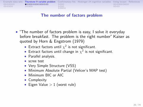
The number of factors problem
• “The number of factors problem is easy, I solve it everydaybefore breakfast. The problem is the right number” Kaiser asquoted by Horn & Engstrom (1979)
• Extract factors until χ2 is not significant.• Extract factors until change in χ2 is not significant.• Parallel analysis.• scree test• Very Simple Structure (VSS)• Minimum Absolute Partial (Velicer’s MAP test)• Minimum BIC or AIC• Complexity• Eigen Value > 1 (worst rule)
20 / 74
Example data sets Thurstone 9 variable problem Confirmatory fits Holzinger 14 cognitive variables Using lavaan References
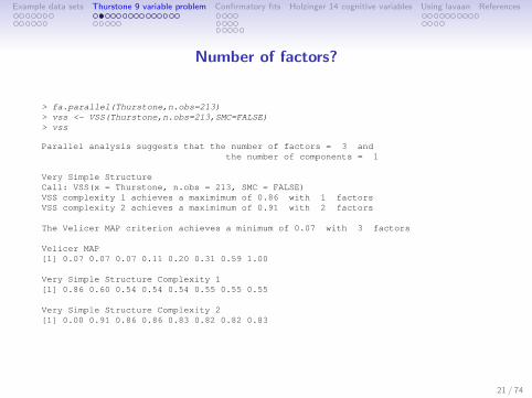
Number of factors?
> fa.parallel(Thurstone,n.obs=213)> vss <- VSS(Thurstone,n.obs=213,SMC=FALSE)> vss
Parallel analysis suggests that the number of factors = 3 andthe number of components = 1
Very Simple StructureCall: VSS(x = Thurstone, n.obs = 213, SMC = FALSE)VSS complexity 1 achieves a maximimum of 0.86 with 1 factorsVSS complexity 2 achieves a maximimum of 0.91 with 2 factors
The Velicer MAP criterion achieves a minimum of 0.07 with 3 factors
Velicer MAP[1] 0.07 0.07 0.07 0.11 0.20 0.31 0.59 1.00
Very Simple Structure Complexity 1[1] 0.86 0.60 0.54 0.54 0.54 0.55 0.55 0.55
Very Simple Structure Complexity 2[1] 0.00 0.91 0.86 0.86 0.83 0.82 0.82 0.83
21 / 74

Example data sets Thurstone 9 variable problem Confirmatory fits Holzinger 14 cognitive variables Using lavaan References
Parallel analysis of the Thurstone data set
2 4 6 8
01
23
45
Parallel Analysis Scree Plots
Factor Number
eige
nval
ues
of p
rinci
pal c
ompo
nent
s an
d fa
ctor
ana
lysi
s
PC Actual Data PC Simulated DataFA Actual Data FA Simulated Data
22 / 74

Example data sets Thurstone 9 variable problem Confirmatory fits Holzinger 14 cognitive variables Using lavaan References
VSS fit function
1
1
1 1 1 1 1 1
1 2 3 4 5 6 7 8
0.0
0.2
0.4
0.6
0.8
1.0
Number of Factors
Ver
y S
impl
e S
truc
ture
Fit
Very Simple Structure
2
2 22 2 2 2
3 3 3 3 3 34 4 4 4 4
23 / 74

Example data sets Thurstone 9 variable problem Confirmatory fits Holzinger 14 cognitive variables Using lavaan References
And many moreR code
nfactors{Thurstone,n.obs=213)
Number of factorsCall: vss(x = x, n = n, rotate = rotate, diagonal = diagonal, fm = fm,
n.obs = n.obs, plot = FALSE, title = title, use = use, cor = cor)VSS complexity 1 achieves a maximimum of 0.86 with 1 factorsVSS complexity 2 achieves a maximimum of 0.91 with 2 factorsThe Velicer MAP achieves a minimum of 0.07 with 3 factorsEmpirical BIC achieves a minimum of -63.76 with 3 factorsSample Size adjusted BIC achieves a minimum of -23.49 with 3 factors
Statistics by number of factorsvss1 vss2 map dof chisq prob sqresid fit RMSEA BIC SABIC complex eChisq SRMR eCRMS eBIC
1 0.86 0.00 0.075 27 2.3e+02 2.1e-34 3.63 0.86 0.19 86.8 172.3 1.0 1.9e+02 1.1e-01 0.128 42.52 0.60 0.91 0.067 19 8.3e+01 5.6e-10 2.26 0.91 0.13 -18.8 41.4 1.4 7.2e+01 6.9e-02 0.094 -29.63 0.54 0.86 0.066 12 2.8e+00 1.0e+00 1.15 0.96 0.00 -61.5 -23.5 1.5 5.8e-01 6.1e-03 0.011 -63.84 0.54 0.86 0.114 6 1.5e+00 9.6e-01 1.10 0.96 0.00 -30.7 -11.7 1.6 3.1e-01 4.5e-03 0.011 -31.95 0.54 0.83 0.195 1 2.4e-01 6.2e-01 1.02 0.96 0.00 -5.1 -1.9 1.7 7.5e-02 2.2e-03 0.013 -5.36 0.55 0.82 0.312 -3 4.8e-07 NA 0.98 0.96 NA NA NA 1.7 1.9e-07 3.6e-06 NA NA7 0.55 0.82 0.590 -6 4.2e-09 NA 0.94 0.96 NA NA NA 1.7 1.5e-09 3.1e-07 NA NA8 0.55 0.83 1.000 -8 0.0e+00 NA 0.86 0.97 NA NA NA 1.7 3.3e-19 4.6e-12 NA NA9 0.55 0.83 NA -9 0.0e+00 NA 0.86 0.97 NA NA NA 1.7 3.2e-27 4.6e-16 NA NA
24 / 74
Example data sets Thurstone 9 variable problem Confirmatory fits Holzinger 14 cognitive variables Using lavaan References
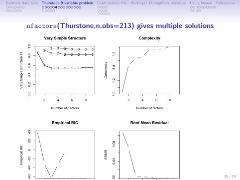
nfactors(Thurstone,n.obs=213) gives multiple solutions
1
11 1 1 1 1 1 1
2 4 6 8
0.0
0.2
0.4
0.6
0.8
1.0
Very Simple Structure
Number of Factors
Ver
y S
impl
e S
truct
ure
Fit 2
2 2 2 2 2 2 2
3 3 3 3 3 3 3
2 4 6 8
1.0
1.2
1.4
1.6
Complexity
Number of factorsComplexity
2 4 6 8
-60
-40
-20
020
40
Empirical BIC
Number of factors
Em
piric
al B
IC
2 4 6 8
0.00
0.04
0.08
Root Mean Residual
Number of factors
SRMR
25 / 74

Example data sets Thurstone 9 variable problem Confirmatory fits Holzinger 14 cognitive variables Using lavaan References
A Very Simple Structure Plot
1
1
1 1 1 1 1 1
1 2 3 4 5 6 7 8
0.0
0.2
0.4
0.6
0.8
1.0
Number of Factors
Ver
y S
impl
e S
truc
ture
Fit
Very Simple Structure
2
2 22 2 2 2
3 3 3 3 3 34 4 4 4 4
26 / 74
Example data sets Thurstone 9 variable problem Confirmatory fits Holzinger 14 cognitive variables Using lavaan References
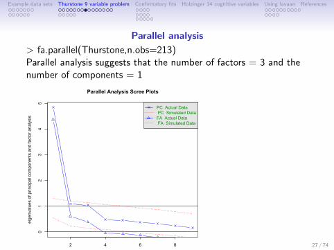
Parallel analysis
> fa.parallel(Thurstone,n.obs=213)Parallel analysis suggests that the number of factors = 3 and thenumber of components = 1
2 4 6 8
01
23
45
Parallel Analysis Scree Plots
Factor Number
eige
nval
ues
of p
rinci
pal c
ompo
nent
s an
d fa
ctor
ana
lysi
s
PC Actual Data PC Simulated DataFA Actual Data FA Simulated Data
27 / 74

Example data sets Thurstone 9 variable problem Confirmatory fits Holzinger 14 cognitive variables Using lavaan References
Minimal Residual FAfa(Thurstone,n.obs=213)
> fa(Thurstone,n.obs=213)Factor Analysis using method = minresCall: fa(r = Thurstone, n.obs = 213)Standardized loadings based upon correlation matrix
MR1 h2 u2V1 0.87 0.75 0.25V2 0.88 0.77 0.23V3 0.83 0.70 0.30V4 0.62 0.39 0.61V5 0.61 0.37 0.63V6 0.59 0.34 0.66V7 0.57 0.32 0.68V8 0.64 0.41 0.59V9 0.52 0.27 0.73
MR1SS loadings 4.32Proportion Var 0.48Test of the hypothesis that 1 factor is sufficient.The degrees of freedom for the null model are 36 and the objective function was 5.2 with Chi Square of 1081.97The degrees of freedom for the model are 27 and the objective function was 1.12The root mean square of the residuals is 0.08The df corrected root mean square of the residuals is 0.13The number of observations was 213 with Chi Square = 231.55 with prob < 2.1e-34Tucker Lewis Index of factoring reliability = 0.738RMSEA index = 0.191 and the 90 % confidence intervals are 0.19 0.194BIC = 86.79Fit based upon off diagonal values = 0.95Measures of factor score adequacy
MR1Correlation of scores with factors 0.96Multiple R square of scores with factors 0.92Minimum correlation of possible factor scores 0.85
28 / 74
Example data sets Thurstone 9 variable problem Confirmatory fits Holzinger 14 cognitive variables Using lavaan References
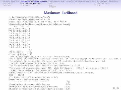
Maximum likelihood> fa(Thurstone,n.obs=213,fm="mle")Factor Analysis using method = mlCall: fa(r = Thurstone, n.obs = 213, fm = "mle")Standardized loadings based upon correlation matrix
ML1 h2 u2V1 0.88 0.78 0.22V2 0.90 0.80 0.20V3 0.85 0.72 0.28V4 0.59 0.35 0.65V5 0.57 0.33 0.67V6 0.57 0.32 0.68V7 0.54 0.29 0.71V8 0.63 0.40 0.60V9 0.49 0.24 0.76
ML1SS loadings 4.22Proportion Var 0.47Test of the hypothesis that 1 factor is sufficient.The degrees of freedom for the null model are 36 and the objective function was 5.2 with Chi Square of 1081.97The degrees of freedom for the model are 27 and the objective function was 1.1The root mean square of the residuals is 0.08The df corrected root mean square of the residuals is 0.14The number of observations was 213 with Chi Square = 228.59 with prob < 8e-34Tucker Lewis Index of factoring reliability = 0.742RMSEA index = 0.19 and the 90 % confidence intervals are 0.189 0.192BIC = 83.83Fit based upon off diagonal values = 0.94Measures of factor score adequacy
ML1Correlation of scores with factors 0.96Multiple R square of scores with factors 0.93Minimum correlation of possible factor scores 0.86 29 / 74

Example data sets Thurstone 9 variable problem Confirmatory fits Holzinger 14 cognitive variables Using lavaan References
Comparing min res and mle
Standardized loadings based upon correlation matrixMR1 h2 u2
V1 0.87 0.75 0.25V2 0.88 0.77 0.23V3 0.83 0.70 0.30V4 0.62 0.39 0.61V5 0.61 0.37 0.63V6 0.59 0.34 0.66V7 0.57 0.32 0.68V8 0.64 0.41 0.59V9 0.52 0.27 0.73
MR1SS loadings 4.32Proportion Var 0.48Chi Square = 231.55
with prob < 2.1e-34
ML1 h2 u2V1 0.88 0.78 0.22V2 0.90 0.80 0.20V3 0.85 0.72 0.28V4 0.59 0.35 0.65V5 0.57 0.33 0.67V6 0.57 0.32 0.68V7 0.54 0.29 0.71V8 0.63 0.40 0.60V9 0.49 0.24 0.76
ML1SS loadings 4.22Proportion Var 0.47Chi Square = 228.59
with prob < 8e-34
30 / 74

Example data sets Thurstone 9 variable problem Confirmatory fits Holzinger 14 cognitive variables Using lavaan References
2 maximum likelihood factors> f2 <- fa(Thurstone,2,n.obs=213,fm="mle")> f2
Factor Analysis using method = mlCall: fa(r = Thurstone, nfactors = 2, n.obs = 213, fm = "mle")Standardized loadings based upon correlation matrix
ML1 ML2 h2 u2V1 0.94 -0.05 0.83 0.17V2 0.89 0.03 0.82 0.18V3 0.85 0.02 0.73 0.27V4 -0.02 0.84 0.68 0.32V5 -0.04 0.84 0.66 0.34V6 0.13 0.59 0.46 0.54V7 0.28 0.35 0.32 0.68V8 0.50 0.17 0.39 0.61V9 0.12 0.49 0.32 0.68
ML1 ML2SS loadings 2.92 2.29Proportion Var 0.32 0.25Cumulative Var 0.32 0.58With factor correlations of
ML1 ML2ML1 1.00 0.64ML2 0.64 1.00 31 / 74

Example data sets Thurstone 9 variable problem Confirmatory fits Holzinger 14 cognitive variables Using lavaan References
2 factor goodness of fits
Test of the hypothesis that 2 factors are sufficient.
The degrees of freedom for the null model are 36 and the objective functionwas 5.2 with Chi Square of 1081.97
The degrees of freedom for the model are 19 and theobjective function was 0.4
The root mean square of the residuals is 0.05The df corrected root mean square of the residuals is 0.1The number of observations was 213 with Chi Square = 82.84
with prob < 6e-10
Tucker Lewis Index of factoring reliability = 0.884RMSEA index = 0.128 and the 90 % confidence intervals are 0.127 0.131BIC = -19.02Fit based upon off diagonal values = 0.98Measures of factor score adequacy
ML1 ML2Correlation of scores with factors 0.97 0.93Multiple R square of scores with factors 0.93 0.86Minimum correlation of possible factor scores 0.86 0.72
32 / 74

Example data sets Thurstone 9 variable problem Confirmatory fits Holzinger 14 cognitive variables Using lavaan References
3 MLE factors of Thurstone data
> f3 <- fa(Thurstone,3,n.obs=213,fm="mle")> f3
Call: fa(r = Thurstone, nfactors = 3, n.obs = 213, fm = "mle")Standardized loadings based upon correlation matrix
ML1 ML2 ML3 h2 u2V1 0.91 -0.04 0.04 0.83 0.17V2 0.89 0.06 -0.03 0.84 0.16V3 0.83 0.04 0.00 0.73 0.27V4 0.00 0.86 0.01 0.73 0.27V5 -0.01 0.74 0.10 0.63 0.37V6 0.18 0.63 -0.08 0.50 0.50V7 0.03 -0.01 0.84 0.72 0.28V8 0.37 -0.05 0.47 0.50 0.50V9 -0.06 0.21 0.64 0.53 0.47
ML1 ML2 ML3SS loadings 2.64 1.86 1.49Proportion Var 0.29 0.21 0.17Cumulative Var 0.29 0.50 0.67With factor correlations of
ML1 ML2 ML3ML1 1.00 0.59 0.54ML2 0.59 1.00 0.52ML3 0.54 0.52 1.00
33 / 74

Example data sets Thurstone 9 variable problem Confirmatory fits Holzinger 14 cognitive variables Using lavaan References
with fit statistics
Test of the hypothesis that 3 factors are sufficient.
The degrees of freedom for the null model are 36 and theobjective function was 5.2 with Chi Square of 1081.97
The degrees of freedom for the model are 12 and theobjective function was 0.01
The root mean square of the residuals is 0The df corrected root mean square of the residuals is 0.01The number of observations was 213 with
Chi Square = 2.82 with prob < 1
Tucker Lewis Index of factoring reliability = 1.027RMSEA index = 0 and the 90 % confidence intervals are 0 0.023BIC = -61.51Fit based upon off diagonal values = 1Measures of factor score adequacy
ML1 ML2 ML3Correlation of scores with factors 0.96 0.92 0.90Multiple R square of scores with factors 0.93 0.85 0.81Minimum correlation of possible factor scores 0.86 0.71 0.63
34 / 74

Example data sets Thurstone 9 variable problem Confirmatory fits Holzinger 14 cognitive variables Using lavaan References
Orthogonal Rotations and oblique Transformations
• Should the latent variables be allowed to correlate?• Factors as extracted are orthogonal.• Factors as interpreted typically are allowed to be oblique
• Consider five cases• unrotated: factors as extracted (rotate=“none”)• rotated using VARIMAX (or Quartimax)• transformed using PROCRUSTES• transformed using oblimin• transformed using geominQ
35 / 74

Example data sets Thurstone 9 variable problem Confirmatory fits Holzinger 14 cognitive variables Using lavaan References
Unrotated versus Varimax Rotation
> fa(Thurstone,3,n.obs=213,rotate="none")
Factor Analysis using method = minresCall: fa(r = Thurstone, nfactors = 3, n.obs = 213, rotate = "none")Standardized loadings based upon correlation matrix
MR1 MR2 MR3 h2 u2V1 0.87 -0.27 0.02 0.82 0.18V2 0.88 -0.24 -0.06 0.84 0.16V3 0.83 -0.22 -0.03 0.73 0.27V4 0.66 0.45 -0.32 0.73 0.27V5 0.63 0.43 -0.21 0.63 0.37V6 0.60 0.24 -0.29 0.50 0.50V7 0.60 0.32 0.50 0.72 0.28V8 0.65 0.05 0.29 0.50 0.50V9 0.54 0.38 0.30 0.53 0.47
MR1 MR2 MR3SS loadings 4.47 0.86 0.67Proportion Var 0.50 0.10 0.07Cumulative Var 0.50 0.59 0.67
> fa(Thurstone,3,n.obs=213,rotate="Varimax")
MR1 MR2 MR3 h2 u2V1 0.86 0.20 0.22 0.82 0.18V2 0.85 0.27 0.18 0.84 0.16V3 0.80 0.24 0.19 0.73 0.27V4 0.29 0.78 0.20 0.73 0.27V5 0.27 0.70 0.26 0.63 0.37V6 0.36 0.60 0.10 0.50 0.50V7 0.28 0.18 0.78 0.72 0.28V8 0.48 0.15 0.50 0.50 0.50V9 0.20 0.32 0.62 0.53 0.47
MR1 MR2 MR3SS loadings 2.73 1.78 1.48Proportion Var 0.30 0.20 0.16Cumulative Var 0.30 0.50 0.67
36 / 74

Example data sets Thurstone 9 variable problem Confirmatory fits Holzinger 14 cognitive variables Using lavaan References
Varimax versus Quartimax
> fa(Thurstone,3,n.obs=213,rotate="Varimax")
MR1 MR2 MR3 h2 u2V1 0.86 0.20 0.22 0.82 0.18V2 0.85 0.27 0.18 0.84 0.16V3 0.80 0.24 0.19 0.73 0.27V4 0.29 0.78 0.20 0.73 0.27V5 0.27 0.70 0.26 0.63 0.37V6 0.36 0.60 0.10 0.50 0.50V7 0.28 0.18 0.78 0.72 0.28V8 0.48 0.15 0.50 0.50 0.50V9 0.20 0.32 0.62 0.53 0.47
MR1 MR2 MR3SS loadings 2.73 1.78 1.48Proportion Var 0.30 0.20 0.16Cumulative Var 0.30 0.50 0.67
> fa(Thurstone,3,n.obs=213,rotate="quartimax")
MR1 MR2 MR3 h2 u2V1 0.91 0.02 0.05 0.82 0.18V2 0.91 0.09 0.01 0.84 0.16V3 0.85 0.07 0.03 0.73 0.27V4 0.47 0.71 0.11 0.73 0.27V5 0.45 0.63 0.18 0.63 0.37V6 0.48 0.51 0.01 0.50 0.50V7 0.45 0.12 0.71 0.72 0.28V8 0.58 0.05 0.40 0.50 0.50V9 0.37 0.27 0.56 0.53 0.47
MR1 MR2 MR3SS loadings 3.70 1.27 1.03Proportion Var 0.41 0.14 0.11Cumulative Var 0.41 0.55 0.67
37 / 74

Example data sets Thurstone 9 variable problem Confirmatory fits Holzinger 14 cognitive variables Using lavaan References
Varimax versus Quartimin
> fa(Thurstone,3,n.obs=213,rotate="Varimax")
MR1 MR2 MR3 h2 u2V1 0.86 0.20 0.22 0.82 0.18V2 0.85 0.27 0.18 0.84 0.16V3 0.80 0.24 0.19 0.73 0.27V4 0.29 0.78 0.20 0.73 0.27V5 0.27 0.70 0.26 0.63 0.37V6 0.36 0.60 0.10 0.50 0.50V7 0.28 0.18 0.78 0.72 0.28V8 0.48 0.15 0.50 0.50 0.50V9 0.20 0.32 0.62 0.53 0.47
MR1 MR2 MR3SS loadings 2.73 1.78 1.48Proportion Var 0.30 0.20 0.16Cumulative Var 0.30 0.50 0.67
> fa(Thurstone,3,n.obs=213,rotate="quartimin")
MR1 MR2 MR3 h2 u2V1 0.91 -0.04 0.04 0.82 0.18V2 0.89 0.06 -0.03 0.84 0.16V3 0.83 0.04 0.00 0.73 0.27V4 0.00 0.86 0.00 0.73 0.27V5 -0.01 0.74 0.10 0.63 0.37V6 0.18 0.63 -0.08 0.50 0.50V7 0.03 -0.01 0.84 0.72 0.28V8 0.37 -0.05 0.47 0.50 0.50V9 -0.06 0.21 0.64 0.53 0.47
MR1 MR2 MR3SS loadings 2.64 1.86 1.50Proportion Var 0.29 0.21 0.17Cumulative Var 0.29 0.50 0.67With factor correlations of
MR1 MR2 MR3MR1 1.00 0.59 0.54MR2 0.59 1.00 0.52MR3 0.54 0.52 1.00
38 / 74

Example data sets Thurstone 9 variable problem Confirmatory fits Holzinger 14 cognitive variables Using lavaan References
Visualizing the difference: Varimax versus quartimin
Orthogonal Rotation
V1
V2
V3
V4
V5
V6
V7
V9
V8
MR1
0.90.90.8
MR20.80.70.6
MR30.80.60.5
Oblique Transformation
V1
V2
V3
V4
V5
V6
V7
V9
V8
MR1
0.90.90.8
MR20.90.70.6
MR30.80.60.5
0.6
0.5
0.5
39 / 74

Example data sets Thurstone 9 variable problem Confirmatory fits Holzinger 14 cognitive variables Using lavaan References
Specifying the parameters in sem using the RAM notation
• Need to specify each path
• Need to specify the error variance paths as well• A short cut can be done by using psych• See the vignette ‘psych for sem‘” for more details
• Apply this to the Thurstone problem
40 / 74

Example data sets Thurstone 9 variable problem Confirmatory fits Holzinger 14 cognitive variables Using lavaan References
create the sem commands by using psychf3 <- fa(Thurstone,3,fm='mle')mod3 <- structure.diagram(f3,cut=.45,errors=TRUE)mod3
Path Parameter Value[1,] "ML1->V1" "F1V1" NA[2,] "ML1->V2" "F1V2" NA[3,] "ML1->V3" "F1V3" NA[4,] "ML2->V4" "F2V4" NA[5,] "ML2->V5" "F2V5" NA[6,] "ML2->V6" "F2V6" NA[7,] "ML3->V7" "F3V7" NA[8,] "ML3->V8" "F3V8" NA[9,] "ML3->V9" "F3V9" NA[10,] "V1<->V1" "x1e" NA[11,] "V2<->V2" "x2e" NA...[18,] "V9<->V9" "x9e" NA[19,] "ML2<->ML1" "rF2F1" NA[20,] "ML3<->ML1" "rF3F1" NA[21,] "ML3<->ML2" "rF3F2" NA[22,] "ML1<->ML1" NA "1"[23,] "ML2<->ML2" NA "1"[24,] "ML3<->ML3" NA "1" 41 / 74

Example data sets Thurstone 9 variable problem Confirmatory fits Holzinger 14 cognitive variables Using lavaan References
Running sem
> rownames(Thurstone) <- colnames(Thurstone) #to get the names to match the modle> sem3 <- sem(mod3,Thurstone,N=213)> summary(sem3,digits=2)
Model Chisquare = 38 Df = 24 Pr(>Chisq) = 0.033Chisquare (null model) = 1102 Df = 36Goodness-of-fit index = 0.96Adjusted goodness-of-fit index = 0.92RMSEA index = 0.053 90% CI: (0.015, 0.083)Bentler-Bonnett NFI = 0.97Tucker-Lewis NNFI = 0.98Bentler CFI = 0.99SRMR = 0.044BIC = -90
Normalized ResidualsMin. 1st Qu. Median Mean 3rd Qu. Max.-0.97 -0.42 0.00 0.04 0.09 1.63
42 / 74

Example data sets Thurstone 9 variable problem Confirmatory fits Holzinger 14 cognitive variables Using lavaan References
With parameter estimatesParameter Estimates
Estimate Std Error z value Pr(>|z|)F1V1 0.90 0.054 16.7 0.0e+00 V1 <--- ML1F1V2 0.91 0.054 17.0 0.0e+00 V2 <--- ML1F1V3 0.86 0.056 15.3 0.0e+00 V3 <--- ML1F2V4 0.84 0.061 13.8 0.0e+00 V4 <--- ML2F2V5 0.80 0.062 12.9 0.0e+00 V5 <--- ML2F2V6 0.70 0.064 10.9 0.0e+00 V6 <--- ML2F3V7 0.78 0.065 12.0 0.0e+00 V7 <--- ML3F3V8 0.72 0.067 10.7 0.0e+00 V8 <--- ML3F3V9 0.70 0.067 10.5 0.0e+00 V9 <--- ML3x1e 0.18 0.028 6.4 1.7e-10 V1 <--> V1x2e 0.16 0.028 5.9 3.0e-09 V2 <--> V2x3e 0.27 0.033 8.0 1.6e-15 V3 <--> V3x4e 0.30 0.051 5.9 2.7e-09 V4 <--> V4x5e 0.36 0.052 7.0 3.4e-12 V5 <--> V5x6e 0.51 0.060 8.4 0.0e+00 V6 <--> V6x7e 0.39 0.062 6.3 2.3e-10 V7 <--> V7x8e 0.48 0.065 7.4 1.8e-13 V8 <--> V8x9e 0.51 0.065 7.7 9.5e-15 V9 <--> V9rF2F1 0.64 0.051 12.6 0.0e+00 ML1 <--> ML2rF3F1 0.67 0.054 12.5 0.0e+00 ML1 <--> ML3rF3F2 0.64 0.059 10.7 0.0e+00 ML2 <--> ML3
Iterations = 36
43 / 74

Example data sets Thurstone 9 variable problem Confirmatory fits Holzinger 14 cognitive variables Using lavaan References
Exploratory bifactor modelomt <- omega(Thurstone)omega.diagram(omt,sl=FALSE)
OmegaCall: omega(m = Thurstone)Alpha: 0.89G.6: 0.91Omega Hierarchical: 0.74Omega H asymptotic: 0.79Omega Total 0.93
Schmid Leiman Factor loadings greater than 0.2g F1* F2* F3* h2 u2 p2
V1 0.71 0.57 0.82 0.18 0.61V2 0.73 0.55 0.84 0.16 0.63V3 0.68 0.52 0.73 0.27 0.63V4 0.65 0.56 0.73 0.27 0.57V5 0.62 0.49 0.63 0.37 0.61V6 0.56 0.41 0.50 0.50 0.63V7 0.59 0.61 0.72 0.28 0.48V8 0.58 0.23 0.34 0.50 0.50 0.66V9 0.54 0.46 0.53 0.47 0.56
With eigenvalues of:g F1* F2* F3*
3.58 0.96 0.74 0.71general/max 3.71 max/min = 1.35
44 / 74
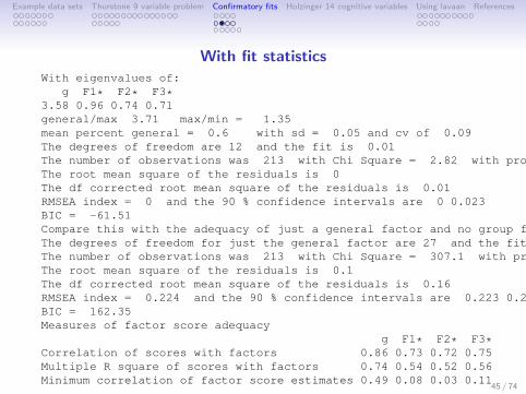
Example data sets Thurstone 9 variable problem Confirmatory fits Holzinger 14 cognitive variables Using lavaan References
With fit statisticsWith eigenvalues of:
g F1* F2* F3*3.58 0.96 0.74 0.71general/max 3.71 max/min = 1.35mean percent general = 0.6 with sd = 0.05 and cv of 0.09The degrees of freedom are 12 and the fit is 0.01The number of observations was 213 with Chi Square = 2.82 with prob < 1The root mean square of the residuals is 0The df corrected root mean square of the residuals is 0.01RMSEA index = 0 and the 90 % confidence intervals are 0 0.023BIC = -61.51Compare this with the adequacy of just a general factor and no group factorsThe degrees of freedom for just the general factor are 27 and the fit is 1.48The number of observations was 213 with Chi Square = 307.1 with prob < 2.8e-49The root mean square of the residuals is 0.1The df corrected root mean square of the residuals is 0.16RMSEA index = 0.224 and the 90 % confidence intervals are 0.223 0.226BIC = 162.35Measures of factor score adequacy
g F1* F2* F3*Correlation of scores with factors 0.86 0.73 0.72 0.75Multiple R square of scores with factors 0.74 0.54 0.52 0.56Minimum correlation of factor score estimates 0.49 0.08 0.03 0.11
45 / 74

Example data sets Thurstone 9 variable problem Confirmatory fits Holzinger 14 cognitive variables Using lavaan References
A correlation plot to show a general factor
Thurstone 9 variable problem
Letter.Group
Pedigrees
Letter.Series
Suffixes
4.Letter.Words
First.Letters
Sent.Completion
Vocabulary
SentencesSntncs
Vcblry
Snt.Cm
Frst.L
4.Lt.W
Suffxs
Lttr.S
Pedgrs
Lttr.G
-1
-0.8
-0.6
-0.4
-0.2
0
0.2
0.4
0.6
0.8
1
46 / 74

Example data sets Thurstone 9 variable problem Confirmatory fits Holzinger 14 cognitive variables Using lavaan References
Two ways of showing a hierarchical structure
Hierarchical (multilevel) Structure
Sentences
Vocabulary
Sent.Completion
First.Letters
4.Letter.Words
Suffixes
Letter.Series
Letter.Group
Pedigrees
F1
0.9
0.9
0.8
0.4
F2
0.9
0.7
0.6
0.2
F30.8
0.6
0.5
g
0.8
0.8
0.7
Omega
Sentences
Vocabulary
Sent.Completion
First.Letters
4.Letter.Words
Suffixes
Letter.Series
Letter.Group
Pedigrees
F1*
0.6
0.6
0.5
0.2
F2*
0.6
0.5
0.4
F3*0.6
0.5
0.3
g
0.7
0.7
0.7
0.6
0.6
0.6
0.6
0.5
0.6
47 / 74

Example data sets Thurstone 9 variable problem Confirmatory fits Holzinger 14 cognitive variables Using lavaan References
Exploratory versus confirmatory bifactor model
• omega will do exploratory bifactoring
• omegaSem will do exploratory and then confirmatory basedupon that solution.
• This is not true “confirmatory” in that the solution was decidedon in an exploratory fashion.
• True confirmatory tests a prior hypothesis
• omegaSem reports both exploratory and confirmatory results.
• The sem model is hidden as part of the structure but may befound from the str command
48 / 74

Example data sets Thurstone 9 variable problem Confirmatory fits Holzinger 14 cognitive variables Using lavaan References
omegaSem
Alpha: 0.89G.6: 0.91Omega Hierarchical: 0.74Omega H asymptotic: 0.79Omega Total 0.93
Schmid Leiman Factor loadings greater than 0.2g F1* F2* F3* h2 u2 p2
Sentences 0.71 0.57 0.82 0.18 0.61Vocabulary 0.73 0.55 0.84 0.16 0.63Sent.Completion 0.68 0.52 0.73 0.27 0.63First.Letters 0.65 0.56 0.73 0.27 0.574.Letter.Words 0.62 0.49 0.63 0.37 0.61Suffixes 0.56 0.41 0.50 0.50 0.63Letter.Series 0.59 0.61 0.72 0.28 0.48Pedigrees 0.58 0.23 0.34 0.50 0.50 0.66Letter.Group 0.54 0.46 0.53 0.47 0.56
With eigenvalues of:g F1* F2* F3*
3.58 0.96 0.74 0.71
Omega Hierarchical from a confirmatory modelusing sem = 0.79
Omega Total from a confirmatory modelusing sem = 0.93
With loadings ofg F1* F2* F3* h2 u2
Sentences 0.77 0.49 0.83 0.17Vocabulary 0.79 0.45 0.83 0.17Sent.Completion 0.75 0.40 0.73 0.27First.Letters 0.61 0.61 0.75 0.254.Letter.Words 0.60 0.51 0.61 0.39Suffixes 0.57 0.39 0.48 0.52Letter.Series 0.57 0.73 0.85 0.15Pedigrees 0.66 0.25 0.50 0.50Letter.Group 0.53 0.41 0.45 0.55
With eigenvalues of:g F1* F2* F3*
3.88 0.61 0.79 0.76
49 / 74

Example data sets Thurstone 9 variable problem Confirmatory fits Holzinger 14 cognitive variables Using lavaan References
The sem model is an object in omegaSem output
omts <- omegaSem(Thurstone,n.obs=213)omts$omegaSem$model
Path Parameter Initial Value[1,] "g->Sentences" "Sentences" NA[2,] "g->Vocabulary" "Vocabulary" NA[...[9,] "g->Letter.Group" "Letter.Group" NA
[10,] "F1*->Sentences" "F1*Sentences" NA[11,] "F1*->Vocabulary" "F1*Vocabulary" NA[12,] "F1*->Sent.Completion" "F1*Sent.Completion" NA[13,] "F2*->First.Letters" "F2*First.Letters" NA[14,] "F2*->4.Letter.Words" "F2*4.Letter.Words" NA[15,] "F2*->Suffixes" "F2*Suffixes" NA[16,] "F3*->Letter.Series" "F3*Letter.Series" NA[17,] "F3*->Pedigrees" "F3*Pedigrees" NA[18,] "F3*->Letter.Group" "F3*Letter.Group" NA[19,] "Sentences<->Sentences" "e1" NA[20,] "Vocabulary<->Vocabulary" "e2" NA...[27,] "Letter.Group<->Letter.Group" "e9" NA[28,] "F1*<->F1*" NA "1"[29,] "F2*<->F2*" NA "1"[30,] "F3*<->F3*" NA "1"[31,] "g <->g" NA "1"
50 / 74

Example data sets Thurstone 9 variable problem Confirmatory fits Holzinger 14 cognitive variables Using lavaan References
Using the sem model from omegaSem
> sem.t.om <- sem(omts$omegaSem$model,Thurstone,N=213)> summary(sem.t.om)
Model Chisquare = 24.216 Df = 18 Pr(>Chisq) = 0.14807Chisquare (null model) = 1101.9 Df = 36Goodness-of-fit index = 0.97578Adjusted goodness-of-fit index = 0.93944RMSEA index = 0.040361 90% CI: (NA, 0.077994)Bentler-Bonnett NFI = 0.97802Tucker-Lewis NNFI = 0.98834Bentler CFI = 0.99417SRMR = 0.034895BIC = -72.287
Normalized ResidualsMin. 1st Qu. Median Mean 3rd Qu. Max.
-0.8210 -0.3340 0.0000 0.0282 0.1560 1.8000
51 / 74

Example data sets Thurstone 9 variable problem Confirmatory fits Holzinger 14 cognitive variables Using lavaan References
sem parameter estimatesParameter Estimates
Estimate Std Error z value Pr(>|z|)Sentences 0.76787 0.072626 10.57291 0.0000e+00 Sentences <--- gVocabulary 0.79092 0.072418 10.92170 0.0000e+00 Vocabulary <--- gSent.Completion 0.75362 0.073402 10.26709 0.0000e+00 Sent.Completion <--- gFirst.Letters 0.60838 0.072201 8.42617 0.0000e+00 First.Letters <--- g4.Letter.Words 0.59733 0.073851 8.08843 6.6613e-16 4.Letter.Words <--- gSuffixes 0.57179 0.071492 7.99792 1.3323e-15 Suffixes <--- gLetter.Series 0.56689 0.074271 7.63282 2.2871e-14 Letter.Series <--- gPedigrees 0.66233 0.069321 9.55455 0.0000e+00 Pedigrees <--- gLetter.Group 0.52995 0.078985 6.70955 1.9522e-11 Letter.Group <--- gF1*Sentences 0.48787 0.085457 5.70898 1.1366e-08 Sentences <--- F1*F1*Vocabulary 0.45232 0.090422 5.00233 5.6640e-07 Vocabulary <--- F1*F1*Sent.Completion 0.40445 0.093402 4.33024 1.4895e-05 Sent.Completion <--- F1*F2*First.Letters 0.61405 0.085794 7.15733 8.2268e-13 First.Letters <--- F2*F2*4.Letter.Words 0.50581 0.084848 5.96130 2.5024e-09 4.Letter.Words <--- F2*F2*Suffixes 0.39432 0.078289 5.03671 4.7359e-07 Suffixes <--- F2*F3*Letter.Series 0.72730 0.159499 4.55988 5.1184e-06 Letter.Series <--- F3*F3*Pedigrees 0.24684 0.089011 2.77317 5.5513e-03 Pedigrees <--- F3*F3*Letter.Group 0.40915 0.122180 3.34875 8.1177e-04 Letter.Group <--- F3*e1 0.17236 0.034113 5.05265 4.3571e-07 Sentences <--> Sentencese2 0.16984 0.030037 5.65438 1.5641e-08 Vocabulary <--> Vocabularye3 0.26847 0.033188 8.08958 6.6613e-16 Sent.Completion <--> Sent.Completione4 0.25281 0.079472 3.18115 1.4669e-03 First.Letters <--> First.Letterse5 0.38735 0.063194 6.12960 8.8103e-10 4.Letter.Words <--> 4.Letter.Wordse6 0.51757 0.059639 8.67838 0.0000e+00 Suffixes <--> Suffixese7 0.14967 0.223242 0.67044 5.0257e-01 Letter.Series <--> Letter.Seriese8 0.50039 0.059655 8.38800 0.0000e+00 Pedigrees <--> Pedigreese9 0.55175 0.084725 6.51223 7.4044e-11 Letter.Group <--> Letter.Group
52 / 74

Example data sets Thurstone 9 variable problem Confirmatory fits Holzinger 14 cognitive variables Using lavaan References
14 cognitive variables from Holzinger
> lowerCor(Holzinger)
T1 T2 T3.4 T6 T28 T29 T32 T34 T35 T36a T13 T18 T25b T77T1 1.00T2 0.52 1.00T3.4 0.49 0.79 1.00T6 0.42 0.42 0.28 1.00T28 0.47 0.28 0.17 0.48 1.00T29 0.33 0.41 0.29 0.62 0.50 1.00T32 -0.44 -0.42 -0.31 -0.57 -0.52 -0.59 1.00T34 -0.11 -0.31 -0.40 0.11 -0.07 -0.13 0.13 1.00T35 -0.23 -0.56 -0.42 -0.15 -0.16 -0.39 0.14 0.41 1.00T36a -0.03 0.02 -0.22 0.20 -0.01 0.13 -0.15 0.40 0.01 1.00T13 0.04 0.59 0.47 0.07 -0.09 0.19 -0.29 -0.45 -0.71 0.02 1.00T18 -0.02 0.54 0.34 0.08 -0.15 0.22 -0.33 -0.46 -0.70 0.08 0.87 1.00T25b -0.03 0.47 0.42 0.01 -0.19 0.07 -0.26 -0.59 -0.68 -0.14 0.81 0.81 1.00T77 -0.01 0.44 0.35 -0.03 -0.15 0.10 -0.26 -0.61 -0.70 -0.13 0.79 0.82 0.79 1.00>
53 / 74

Example data sets Thurstone 9 variable problem Confirmatory fits Holzinger 14 cognitive variables Using lavaan References
14 cognitive variables from Holzinger and Swineford
T77
T25b
T18
T13
T36a
T35
T34
T32
T29
T28
T6
T3.4
T2
T1
T1 T2
T3.4 T6 T28
T29
T32
T34
T35
T36a T13
T18
T25b T77
-1
-0.8
-0.6
-0.4
-0.2
0
0.2
0.4
0.6
0.8
1
54 / 74
Example data sets Thurstone 9 variable problem Confirmatory fits Holzinger 14 cognitive variables Using lavaan References
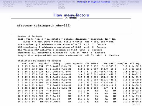
How many factorsR code
nfactors(Holzinger,n.obs=355)
Number of factorsCall: vss(x = x, n = n, rotate = rotate, diagonal = diagonal, fm = fm,
n.obs = n.obs, plot = FALSE, title = title, use = use, cor = cor)VSS complexity 1 achieves a maximimum of 0.75 with 1 factorsVSS complexity 2 achieves a maximimum of 0.83 with 2 factorsThe Velicer MAP achieves a minimum of 0.03 with 2 factorsEmpirical BIC achieves a minimum of -221.54 with 4 factorsSample Size adjusted BIC achieves a minimum of -69.03 with 4 factors
Statistics by number of factorsvss1 vss2 map dof chisq prob sqresid fit RMSEA BIC SABIC complex eChisq SRMR eCRMS eBIC
1 0.75 0.00 0.034 77 5.4e+02 2.6e-71 8.8 0.75 0.132 91.2 335.5 1.0 7.1e+02 1.0e-01 0.114 255.92 0.59 0.83 0.026 64 2.3e+02 7.3e-21 5.9 0.83 0.087 -144.0 59.1 1.4 2.3e+02 5.9e-02 0.070 -150.13 0.56 0.82 0.029 52 1.2e+02 4.7e-07 4.5 0.87 0.061 -187.3 -22.3 1.5 8.6e+01 3.7e-02 0.048 -218.94 0.51 0.77 0.036 41 4.2e+01 4.4e-01 3.6 0.90 0.011 -199.1 -69.0 1.7 1.9e+01 1.7e-02 0.026 -221.55 0.49 0.73 0.061 31 2.7e+01 6.6e-01 3.5 0.90 0.000 -154.9 -56.5 1.8 1.3e+01 1.4e-02 0.024 -169.56 0.48 0.70 0.071 22 1.4e+01 9.2e-01 3.0 0.91 0.000 -115.6 -45.8 1.9 6.0e+00 9.6e-03 0.020 -123.27 0.44 0.62 0.102 14 5.8e+00 9.7e-01 2.9 0.92 0.000 -76.4 -32.0 2.1 3.0e+00 6.8e-03 0.017 -79.28 0.44 0.61 0.141 7 2.7e+00 9.2e-01 2.8 0.92 0.000 -38.5 -16.2 2.1 1.6e+00 5.0e-03 0.018 -39.59 0.45 0.62 0.183 1 1.9e-01 6.6e-01 2.4 0.93 0.000 -5.7 -2.5 1.9 1.2e-01 1.4e-03 0.013 -5.810 0.46 0.67 0.235 -4 9.9e-02 NA 2.2 0.94 NA NA NA 1.9 5.1e-02 8.9e-04 NA NA11 0.43 0.61 0.369 -8 1.9e-07 NA 2.2 0.94 NA NA NA 2.1 1.0e-07 1.3e-06 NA NA12 0.43 0.65 0.529 -11 1.0e-08 NA 2.3 0.93 NA NA NA 2.1 5.1e-09 2.8e-07 NA NA13 0.43 0.64 1.000 -13 6.0e-13 NA 2.3 0.93 NA NA NA 2.2 3.5e-16 7.4e-11 NA NA14 0.43 0.64 NA -14 0.0e+00 NA 2.3 0.93 NA NA NA 2.2 2.3e-26 5.9e-16 NA NA
55 / 74

Example data sets Thurstone 9 variable problem Confirmatory fits Holzinger 14 cognitive variables Using lavaan References
Holzinger 14 variable problem
1
1
1 1 1 1 1 1
1 2 3 4 5 6 7 8
0.0
0.2
0.4
0.6
0.8
1.0
Number of Factors
Ver
y S
impl
e S
truct
ure
Fit
Very Simple Structure
2
2 22 2 2 2
3 3 3 3 3 34 4 4 4 4
56 / 74

Example data sets Thurstone 9 variable problem Confirmatory fits Holzinger 14 cognitive variables Using lavaan References
Parallel analysis of Holzinger 14 variables
> fa.parallel(Holzinger,n.obs=355) Parallel analysis suggests thatthe number of factors = 4 and the number of components = 3
2 4 6 8 10 12 14
01
23
45
Parallel Analysis Scree Plots
Factor Number
eige
nval
ues
of p
rinci
pal c
ompo
nent
s an
d fa
ctor
ana
lysi
s
PC Actual Data PC Simulated DataFA Actual Data FA Simulated Data
57 / 74

Example data sets Thurstone 9 variable problem Confirmatory fits Holzinger 14 cognitive variables Using lavaan References
Exploratory Omega solution for Holzinger 14 variable problem
Holzinger 14 cognitive variables
T18
T13
T77
T25b
T29
T28
T6
T34
T36a
T35
T32
T3.4
T2
T1
F1
0.90.70.70.7
0.3-0.2
0.2
F20.60.60.6
-0.3
0.20.4
F30.70.50.50.4
F40.80.50.4
g
0.7
0.7
0.4
0.7
Holzinger 14 cognitive variables
T18
T13
T77
T25b
T29
T28
T6
T34
T36a
T35
T32
T3.4
T2
T1
F1*
0.70.60.60.5
0.2 F2*0.50.40.4
-0.2
0.3
F3*0.70.40.40.4
F4*0.60.30.3
g
0.60.60.50.50.50.40.60.30.4
0.70.70.5
58 / 74
Example data sets Thurstone 9 variable problem Confirmatory fits Holzinger 14 cognitive variables Using lavaan References
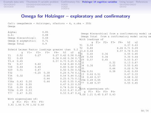
Omega for Holzinger – exploratory and confirmatory
Call: omegaSem(m = Holzinger, nfactors = 4, n.obs = 355)Omega
Alpha: 0.85G.6: 0.88Omega Hierarchical: 0.64Omega H asymptotic: 0.71Omega Total 0.9
Schmid Leiman Factor loadings greater than 0.2g F1* F2* F3* F4* h2 u2 p2
T1 0.52 0.27 0.27 0.42 0.58 0.64T2 0.69 0.34 0.66 0.34 0.72T3.4 0.65 0.57 0.75 0.25 0.56T6 0.57 0.42 0.54 0.46 0.59T28 0.44 0.44 0.40 0.60 0.49T29 0.51 0.47 0.50 0.50 0.54T32 -0.25 0.38 0.26 0.74 0.13T34 0.32 0.66 0.54 0.46 0.19T35 0.44 0.25 0.75 0.10T36a 0.43 0.20 0.44 0.45 0.55 0.41T13 0.59 0.55 0.67 0.33 0.52T18 0.55 0.65 0.74 0.26 0.42T25b 0.49 0.53 0.53 0.47 0.43T77 0.47 0.55 0.53 0.47 0.41
With eigenvalues of:g F1* F2* F3* F4*
3.41 1.44 0.78 1.02 0.58
Omega Hierarchical from a confirmatory model using sem = 0.75Omega Total from a confirmatory model using sem = 0.9
With loadings ofg F1* F2* F3* F4* h2 u2
T1 0.59 0.37 0.63T2 0.80 0.26 0.71 0.29T3.4 0.64 0.57 0.74 0.26T6 0.65 0.36 0.55 0.45T28 0.50 0.34 0.36 0.64T29 0.57 0.45 0.53 0.47T32 0.32 0.13 0.87T34 0.36 0.65 0.55 0.45T35 0.44 0.22 0.78T36a 0.51 0.38 0.41 0.59T13 0.64 0.51 0.67 0.33T18 0.60 0.57 0.68 0.32T25b 0.49 0.55 0.55 0.45T77 0.48 0.57 0.55 0.45
With eigenvalues of:g F1* F2* F3* F4*
4.06 1.21 0.45 0.87 0.43
59 / 74
Example data sets Thurstone 9 variable problem Confirmatory fits Holzinger 14 cognitive variables Using lavaan References
lavaan: Latent Variable Analysis
• The lavaan package Rosseel (2012) is a very powerful sem/cfamodeling package.
• Mimics input of LISREL and MPlus• Easier to set up than sem Fox, Nie & Byrnes (2013)• Clearly targets MPlus• Further help available at http://lavaan.ugent.be/• Example data sets from MPlus
60 / 74
Example data sets Thurstone 9 variable problem Confirmatory fits Holzinger 14 cognitive variables Using lavaan References
An example from lavaan
1. Holzinger Swineford data set from three schools• First describe the data• descriptive stats and graphics
2. Then consider the structure of the 9 variables• Using fa• Using sem/lavaan
61 / 74
Example data sets Thurstone 9 variable problem Confirmatory fits Holzinger 14 cognitive variables Using lavaan References
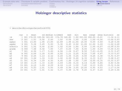
Holzinger descriptive statistics
> describe(HolzingerSwineford1939)
var n mean sd median trimmed mad min max range skew kurtosis seid 1 301 176.55 105.94 163.00 176.78 140.85 1.00 351.00 350.00 -0.01 -1.36 6.11sex 2 301 1.51 0.50 2.00 1.52 0.00 1.00 2.00 1.00 -0.06 -2.00 0.03ageyr 3 301 13.00 1.05 13.00 12.89 1.48 11.00 16.00 5.00 0.69 0.20 0.06agemo 4 301 5.38 3.45 5.00 5.32 4.45 0.00 11.00 11.00 0.09 -1.22 0.20school* 5 301 1.52 0.50 2.00 1.52 0.00 1.00 2.00 1.00 -0.07 -2.00 0.03grade 6 300 7.48 0.50 7.00 7.47 0.00 7.00 8.00 1.00 0.09 -2.00 0.03x1 7 301 4.94 1.17 5.00 4.96 1.24 0.67 8.50 7.83 -0.25 0.31 0.07x2 8 301 6.09 1.18 6.00 6.02 1.11 2.25 9.25 7.00 0.47 0.33 0.07x3 9 301 2.25 1.13 2.12 2.20 1.30 0.25 4.50 4.25 0.38 -0.91 0.07x4 10 301 3.06 1.16 3.00 3.02 0.99 0.00 6.33 6.33 0.27 0.08 0.07x5 11 301 4.34 1.29 4.50 4.40 1.48 1.00 7.00 6.00 -0.35 -0.55 0.07x6 12 301 2.19 1.10 2.00 2.09 1.06 0.14 6.14 6.00 0.86 0.82 0.06x7 13 301 4.19 1.09 4.09 4.16 1.10 1.30 7.43 6.13 0.25 -0.31 0.06x8 14 301 5.53 1.01 5.50 5.49 0.96 3.05 10.00 6.95 0.53 1.17 0.06x9 15 301 5.37 1.01 5.42 5.37 0.99 2.78 9.25 6.47 0.20 0.29 0.06
62 / 74

Example data sets Thurstone 9 variable problem Confirmatory fits Holzinger 14 cognitive variables Using lavaan References
Pairs panels of HolzingerSwineford1939
x12 5 8
0.30 0.44
0 2 4 6
0.37 0.29
0 2 4 6
0.36 0.07
3 6 9
0.22
260.39
25
8 x20.34 0.15 0.14 0.19 -0.08 0.09 0.21
x30.16 0.08 0.20 0.07 0.19
130.33
0246 x40.73 0.70 0.17 0.11 0.21
x50.72 0.10 0.14
1357
0.23
0246 x6
0.12 0.15 0.21
x70.49
246
0.34
36
9 x80.45
2 6 1 3 1 3 5 7 2 4 6 3 6 9
36
9x963 / 74

Example data sets Thurstone 9 variable problem Confirmatory fits Holzinger 14 cognitive variables Using lavaan References
Weaker correlations than the Thurstone data set
Holzinger Swineford datax9
x8x7
x6x5
x4x3
x2x1
x1 x2 x3 x4 x5 x6 x7 x8 x9
-1
-0.8
-0.6
-0.4
-0.2
0
0.2
0.4
0.6
0.8
1
64 / 74

Example data sets Thurstone 9 variable problem Confirmatory fits Holzinger 14 cognitive variables Using lavaan References
Parallel Analysis of the Holzlinger Swineford data set
2 4 6 8
0.0
0.5
1.0
1.5
2.0
2.5
3.0
Parallel Analysis Scree Plots
Factor Number
eige
nval
ues
of p
rinci
pal c
ompo
nent
s an
d fa
ctor
ana
lysi
s
PC Actual Data PC Simulated Data PC Resampled Data FA Actual Data FA Simulated Data FA Resampled Data
65 / 74
Example data sets Thurstone 9 variable problem Confirmatory fits Holzinger 14 cognitive variables Using lavaan References
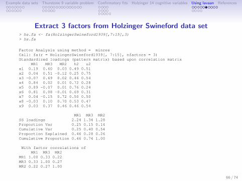
Extract 3 factors from Holzinger Swineford data set> hs.fa <- fa(HolzingerSwineford1939[,7:15],3)> hs.fa
Factor Analysis using method = minresCall: fa(r = HolzingerSwineford1939[, 7:15], nfactors = 3)Standardized loadings (pattern matrix) based upon correlation matrix
MR1 MR3 MR2 h2 u2x1 0.19 0.60 0.03 0.49 0.51x2 0.04 0.51 -0.12 0.25 0.75x3 -0.07 0.69 0.02 0.46 0.54x4 0.84 0.02 0.01 0.72 0.28x5 0.89 -0.07 0.01 0.76 0.24x6 0.81 0.08 -0.01 0.69 0.31x7 0.04 -0.15 0.72 0.50 0.50x8 -0.03 0.10 0.70 0.53 0.47x9 0.03 0.37 0.46 0.46 0.54
MR1 MR3 MR2SS loadings 2.24 1.34 1.28Proportion Var 0.25 0.15 0.14Cumulative Var 0.25 0.40 0.54Proportion Explained 0.46 0.28 0.26Cumulative Proportion 0.46 0.74 1.00
With factor correlations ofMR1 MR3 MR2
MR1 1.00 0.33 0.22MR3 0.33 1.00 0.27MR2 0.22 0.27 1.00
66 / 74

Example data sets Thurstone 9 variable problem Confirmatory fits Holzinger 14 cognitive variables Using lavaan References
With goodness of fit stats
Test of the hypothesis that 3 factors are sufficient.
The degrees of freedom for the null model are 36 and the objective function was 3.05 with Chi Square of 904.1The degrees of freedom for the model are 12 and the objective function was 0.08
The root mean square of the residuals (RMSR) is 0.01The df corrected root mean square of the residuals is 0.03The number of observations was 301 with Chi Square = 22.38 with prob < 0.034
Tucker Lewis Index of factoring reliability = 0.964RMSEA index = 0.055 and the 90 % confidence intervals are 0.015 0.088BIC = -46.11Fit based upon off diagonal values = 1Measures of factor score adequacy
MR1 MR3 MR2Correlation of scores with factors 0.94 0.84 0.85Multiple R square of scores with factors 0.89 0.71 0.72Minimum correlation of possible factor scores 0.78 0.42 0.45
67 / 74

Example data sets Thurstone 9 variable problem Confirmatory fits Holzinger 14 cognitive variables Using lavaan References
Weak evidence for hierarchical structure
Omega
x5
x4
x6
x3
x1
x2
x7
x8
x9
F1*
0.80.70.7
F2*0.50.50.4
0.3F3*
0.70.60.4
g
0.40.40.50.40.50.30.20.30.4
68 / 74
Example data sets Thurstone 9 variable problem Confirmatory fits Holzinger 14 cognitive variables Using lavaan References
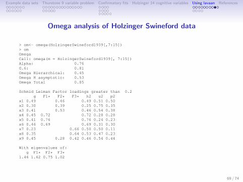
Omega analysis of Holzinger Swineford data
> om<- omega(HolzingerSwineford1939[,7:15])> omOmegaCall: omega(m = HolzingerSwineford1939[, 7:15])Alpha: 0.76G.6: 0.81Omega Hierarchical: 0.45Omega H asymptotic: 0.53Omega Total 0.85
Schmid Leiman Factor loadings greater than 0.2g F1* F2* F3* h2 u2 p2
x1 0.49 0.46 0.49 0.51 0.50x2 0.30 0.39 0.25 0.75 0.35x3 0.41 0.53 0.46 0.54 0.38x4 0.45 0.72 0.72 0.28 0.28x5 0.41 0.76 0.76 0.24 0.23x6 0.46 0.69 0.69 0.31 0.30x7 0.23 0.66 0.50 0.50 0.11x8 0.35 0.64 0.53 0.47 0.23x9 0.45 0.28 0.42 0.46 0.54 0.44
With eigenvalues of:g F1* F2* F3*
1.46 1.62 0.75 1.02
69 / 74

Example data sets Thurstone 9 variable problem Confirmatory fits Holzinger 14 cognitive variables Using lavaan References
Omega fit statistics for Holzinger Swineford
general/max 0.9 max/min = 2.15mean percent general = 0.31 with sd = 0.12 and cv of 0.38
The degrees of freedom are 12 and the fit is 0.08The number of observations was 301 with Chi Square = 22.38 with prob < 0.034The root mean square of the residuals is 0.01The df corrected root mean square of the residuals is 0.03RMSEA index = 0.055 and the 90 % confidence intervals are 0.015 0.088BIC = -46.11
Compare this with the adequacy of just a general factor and no group factorsThe degrees of freedom for just the general factor are 27 and the fit is 1.75The number of observations was 301 with Chi Square = 517.18 with prob < 4.4e-92The root mean square of the residuals is 0.14The df corrected root mean square of the residuals is 0.23
RMSEA index = 0.248 and the 90 % confidence intervals are 0.227 0.264BIC = 363.09
Measures of factor score adequacyg F1* F2* F3*
Correlation of scores with factors 0.68 0.84 0.67 0.78Multiple R square of scores with factors 0.46 0.71 0.44 0.61Minimum correlation of factor score estimates -0.07 0.43 -0.11 0.22
70 / 74

Example data sets Thurstone 9 variable problem Confirmatory fits Holzinger 14 cognitive variables Using lavaan References
The lavaan commands
# The Holzinger and Swineford (1939) exampleHS.model <- ' visual =~ x1 + x2 + x3
textual =~ x4 + x5 + x6speed =~ x7 + x8 + x9 '
fit <- lavaan(HS.model, data=HolzingerSwineford1939,auto.var=TRUE, auto.fix.first=TRUE,auto.cov.lv.x=TRUE)
summary(fit, fit.measures=TRUE)
71 / 74

Example data sets Thurstone 9 variable problem Confirmatory fits Holzinger 14 cognitive variables Using lavaan References
lavaan output
lavaan (0.4-14) converged normally after 41 iterations
Number of observations 301
Estimator MLMinimum Function Chi-square 85.306Degrees of freedom 24P-value 0.000
Chi-square test baseline model:Minimum Function Chi-square 918.852Degrees of freedom 36P-value 0.000
Full model versus baseline model:Comparative Fit Index (CFI) 0.931Tucker-Lewis Index (TLI) 0.896
Loglikelihood and Information Criteria:Loglikelihood user model (H0) -3737.745Loglikelihood unrestricted model (H1) -3695.092Number of free parameters 21Akaike (AIC) 7517.490Bayesian (BIC) 7595.339Sample-size adjusted Bayesian (BIC) 7528.739
Root Mean Square Error of Approximation:RMSEA 0.09290 Percent Confidence Interval 0.071 0.114P-value RMSEA <= 0.05 0.001
72 / 74
Example data sets Thurstone 9 variable problem Confirmatory fits Holzinger 14 cognitive variables Using lavaan References
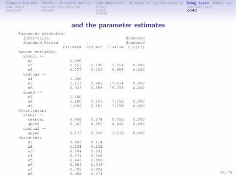
and the parameter estimatesParameter estimates:
Information ExpectedStandard Errors Standard
Estimate Std.err Z-value P(>|z|)Latent variables:
visual =~x1 1.000x2 0.553 0.100 5.554 0.000x3 0.729 0.109 6.685 0.000
textual =~x4 1.000x5 1.113 0.065 17.014 0.000x6 0.926 0.055 16.703 0.000
speed =~x7 1.000x8 1.180 0.165 7.152 0.000x9 1.082 0.151 7.155 0.000
Covariances:visual ~~
textual 0.408 0.074 5.552 0.000speed 0.262 0.056 4.660 0.000
textual ~~speed 0.173 0.049 3.518 0.000
Variances:x1 0.549 0.114x2 1.134 0.102x3 0.844 0.091x4 0.371 0.048x5 0.446 0.058x6 0.356 0.043x7 0.799 0.081x8 0.488 0.074x9 0.566 0.071visual 0.809 0.145textual 0.979 0.112speed 0.384 0.086
73 / 74
Example data sets Thurstone 9 variable problem Confirmatory fits Holzinger 14 cognitive variables Using lavaan References
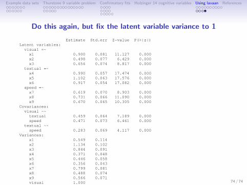
Do this again, but fix the latent variable variance to 1
Estimate Std.err Z-value P(>|z|)Latent variables:
visual =~x1 0.900 0.081 11.127 0.000x2 0.498 0.077 6.429 0.000x3 0.656 0.074 8.817 0.000
textual =~x4 0.990 0.057 17.474 0.000x5 1.102 0.063 17.576 0.000x6 0.917 0.054 17.082 0.000
speed =~x7 0.619 0.070 8.903 0.000x8 0.731 0.066 11.090 0.000x9 0.670 0.065 10.305 0.000
Covariances:visual ~~
textual 0.459 0.064 7.189 0.000speed 0.471 0.073 6.461 0.000
textual ~~speed 0.283 0.069 4.117 0.000
Variances:x1 0.549 0.114x2 1.134 0.102x3 0.844 0.091x4 0.371 0.048x5 0.446 0.058x6 0.356 0.043x7 0.799 0.081x8 0.488 0.074x9 0.566 0.071visual 1.000textual 1.000speed 1.000
74 / 74

Example data sets Thurstone 9 variable problem Confirmatory fits Holzinger 14 cognitive variables Using lavaan References
Bechtoldt, H. (1961). An empirical study of the factor analysisstability hypothesis. Psychometrika, 26(4), 405–432.
Fox, J., Nie, Z., & Byrnes, J. (2013). sem: Structural EquationModels. R package version 3.1-3.
Horn, J. L. & Engstrom, R. (1979). Cattell’s scree test in relationto bartlett’s chi-square test and other observations on thenumber of factors problem. Multivariate Behavioral Research,14(3), 283–300.
McDonald, R. P. (1999). Test theory: A unified treatment.Mahwah, N.J.: L. Erlbaum Associates.
Rosseel, Y. (2012). lavaan: An R package for structural equationmodeling. Journal of Statistical Software, 48(2), 1–36.
Thurstone, L. L. & Thurstone, T. G. (1941). Factorial studies ofintelligence. Chicago, Ill.: The University of Chicago press.
74 / 74