Psy B07 Chapter 9Slide 1 CORRELATION & REGRESSION.
44
Chapter 9 Chapter 9 Slide Slide 1 Psy B07 CORRELATION & REGRESSION CORRELATION & REGRESSION
-
Upload
liliana-alexander -
Category
Documents
-
view
226 -
download
1
Transcript of Psy B07 Chapter 9Slide 1 CORRELATION & REGRESSION.
Chapter 9Chapter 9 Slide Slide 11
Psy B07
CORRELATION & CORRELATION & REGRESSIONREGRESSION
Chapter 9Chapter 9 Slide Slide 22
Psy B07
Correlation vs. RegressionCorrelation vs. Regression
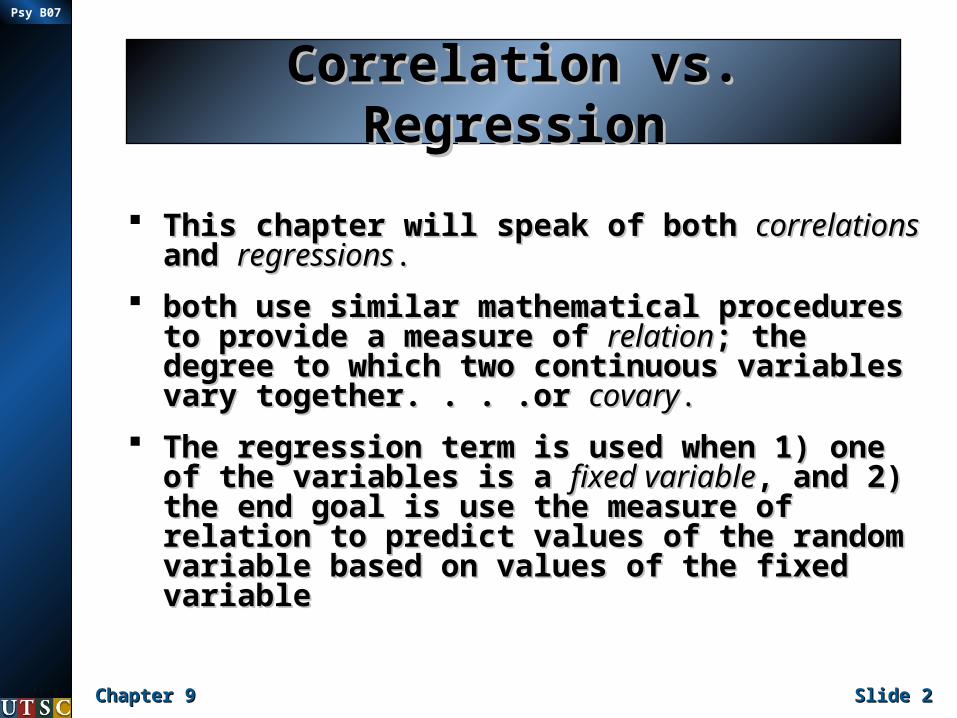
This chapter will speak of both This chapter will speak of both correlationscorrelations and and regressionsregressions..
both use similar mathematical procedures both use similar mathematical procedures to provide a measure of to provide a measure of relationrelation; the ; the degree to which two continuous variables degree to which two continuous variables vary together. . . .or vary together. . . .or covarycovary..
The regression term is used when 1) one The regression term is used when 1) one of the variables is a of the variables is a fixed variablefixed variable, and 2) , and 2) the end goal is use the measure of relation the end goal is use the measure of relation to predict values of the random variable to predict values of the random variable based on values of the fixed variablebased on values of the fixed variable
Chapter 9Chapter 9 Slide Slide 33
Psy B07
Correlation vs. RegressionCorrelation vs. Regression
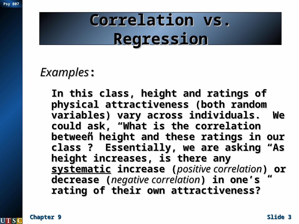
ExamplesExamples::
In this class, height and ratings of In this class, height and ratings of physical attractiveness (both random physical attractiveness (both random variables) vary across individuals. We variables) vary across individuals. We could ask, “What is the correlation could ask, “What is the correlation between height and these ratings in our between height and these ratings in our class”? Essentially, we are asking “As class”? Essentially, we are asking “As height increases, is there any height increases, is there any systematicsystematic increase (increase (positive correlationpositive correlation) or decrease ) or decrease ((negative correlationnegative correlation) in one’s rating of ) in one’s rating of their own attractiveness?”their own attractiveness?”
Chapter 9Chapter 9 Slide Slide 44
Psy B07
Correlation vs. RegressionCorrelation vs. Regression
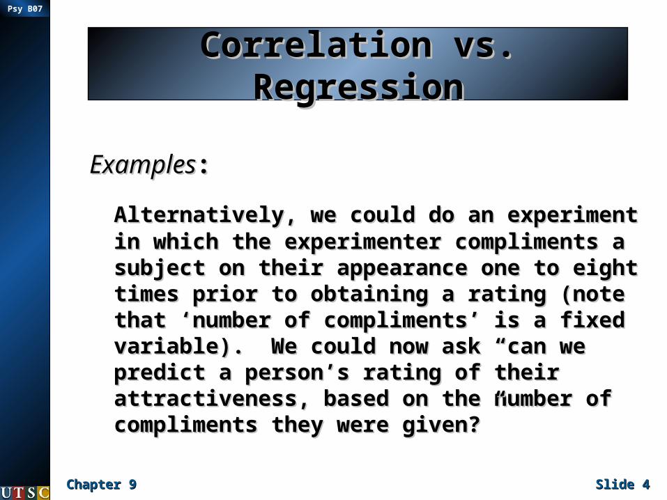
ExamplesExamples::
Alternatively, we could do an experiment Alternatively, we could do an experiment in which the experimenter compliments a in which the experimenter compliments a subject on their appearance one to eight subject on their appearance one to eight times prior to obtaining a rating (note times prior to obtaining a rating (note that ‘number of compliments’ is a fixed that ‘number of compliments’ is a fixed variable). We could now ask “can we variable). We could now ask “can we predict a person’s rating of their predict a person’s rating of their attractiveness, based on the number of attractiveness, based on the number of compliments they were given?”compliments they were given?”
Chapter 9Chapter 9 Slide Slide 55
Psy B07
ScatterplotsScatterplots
The first way to get some idea The first way to get some idea about a possible relation between about a possible relation between two variables is to do a scatterplot two variables is to do a scatterplot of the variables.of the variables.
Let’s consider the first example Let’s consider the first example discussed previously where we discussed previously where we were interested in the possible were interested in the possible relation between height and relation between height and ratings of physical attractiveness.ratings of physical attractiveness.
Chapter 9Chapter 9 Slide Slide 66
Psy B07
ScatterplotsScatterplots
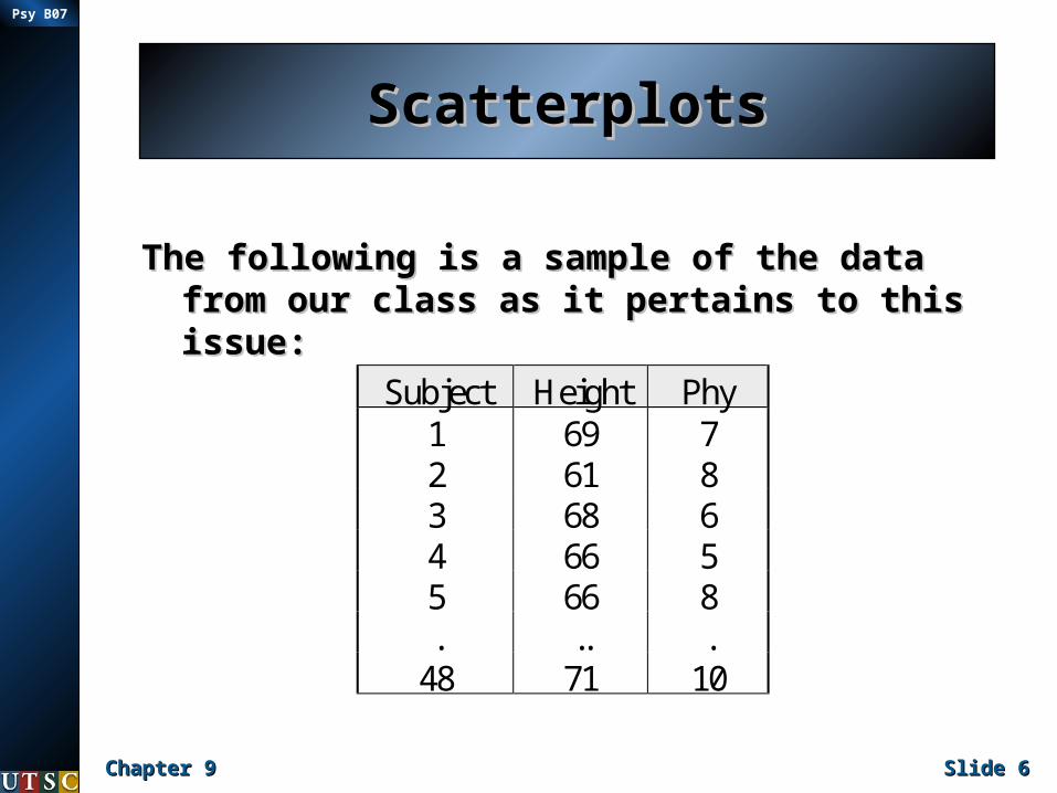
The following is a sample of the data from The following is a sample of the data from our class as it pertains to this issue:our class as it pertains to this issue:
Subject Height Phy1 69 72 61 83 68 64 66 55 66 8. .. .
48 71 10
Chapter 9Chapter 9 Slide Slide 77
Psy B07
ScatterplotsScatterplots
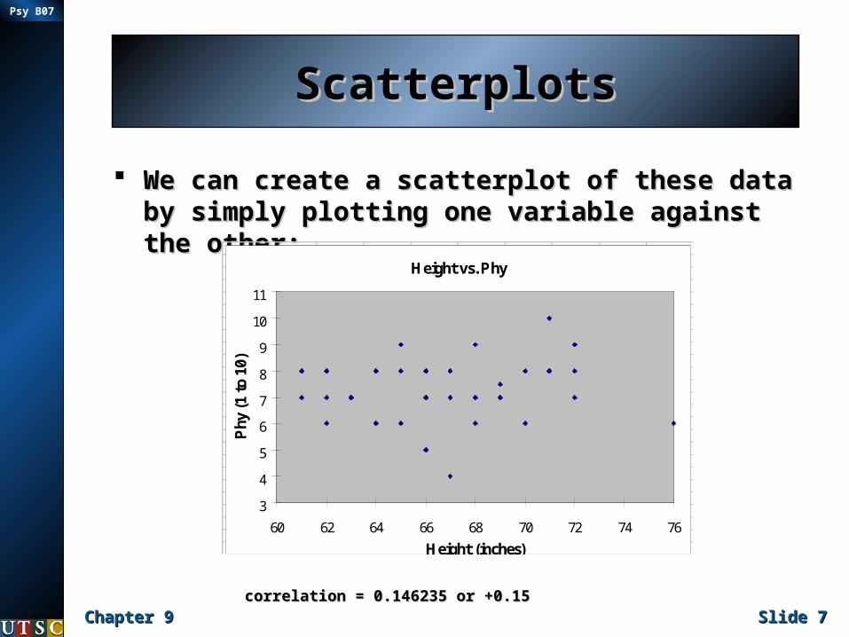
We can create a scatterplot of these data We can create a scatterplot of these data by simply plotting one variable against the by simply plotting one variable against the other:other:
correlation = 0.146235 or +0.15correlation = 0.146235 or +0.15
69 761 868 666 566 863 772 962 762 867 866 563 767 465 672 761 763 766 768 762 868 972 867 766 766 8
Height vs. Phy
3
4
5
6
7
8
9
10
11
60 62 64 66 68 70 72 74 76
Height (inches)
Phy
(1
to 1
0)
Chapter 9Chapter 9 Slide Slide 88
Psy B07
ScatterplotsScatterplots
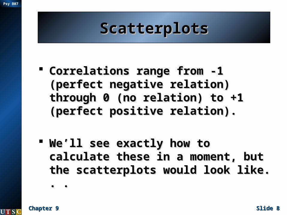
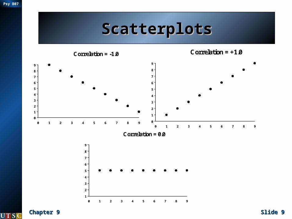
Correlations range from -1 (perfect Correlations range from -1 (perfect negative relation) through 0 (no negative relation) through 0 (no relation) to +1 (perfect positive relation) to +1 (perfect positive relation).relation).
We’ll see exactly how to calculate We’ll see exactly how to calculate these in a moment, but the these in a moment, but the scatterplots would look like. . .scatterplots would look like. . .
Chapter 9Chapter 9 Slide Slide 99
Psy B07
ScatterplotsScatterplots Correlation = -1.0
0
1
2
3
4
5
6
7
8
9
0 1 2 3 4 5 6 7 8 9
Correlation = +1.0
0
1
2
3
4
5
6
7
8
9
0 1 2 3 4 5 6 7 8 9
Correlation = 0.0
1
2
3
4
5
6
7
8
9
0 1 2 3 4 5 6 7 8 9
Chapter 9Chapter 9 Slide Slide 1010
Psy B07
CovarianceCovariance
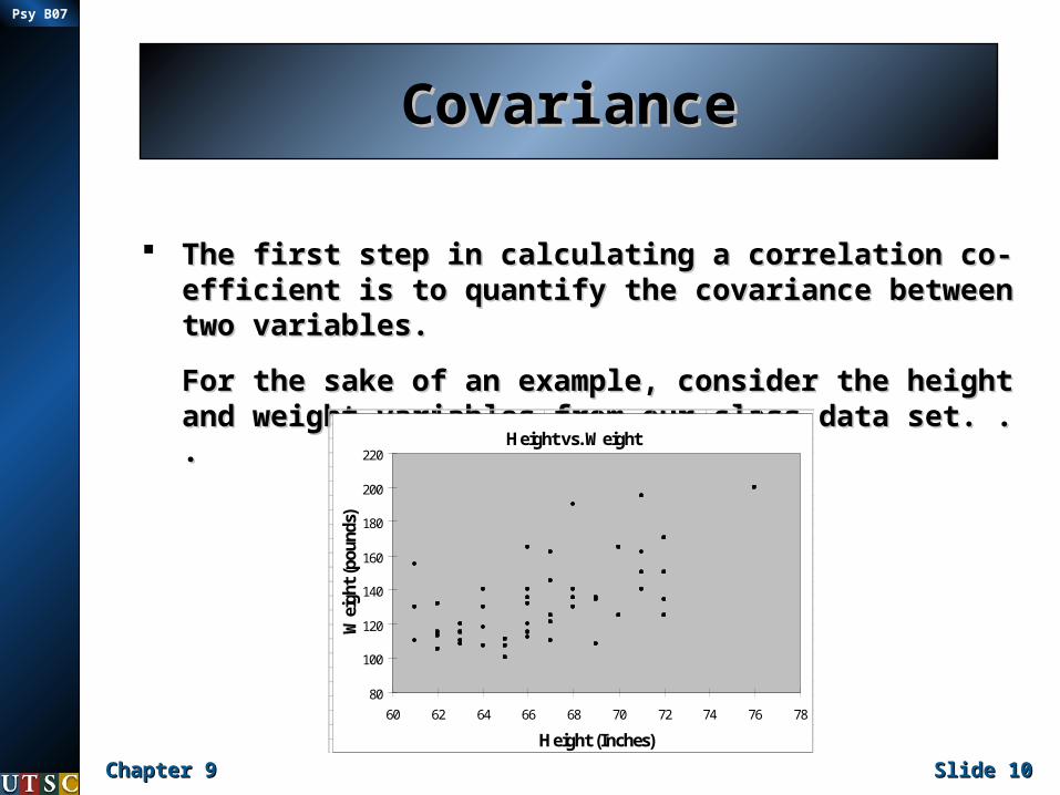
The first step in calculating a correlation co-The first step in calculating a correlation co-efficient is to quantify the covariance between efficient is to quantify the covariance between two variables.two variables.
For the sake of an example, consider the height For the sake of an example, consider the height and weight variables from our class data set. . .and weight variables from our class data set. . .1 1 19 69 108 1 2.5 1.5 7
2 0 18 61 130 1 4 0 83 1 20 68 135 3 5 1 64 0 21 66 135 3 6 0 55 0 26 66 120 1 0 0 86 0 21 63 115 2 4 0 77 1 18 72 150 3 40 0 98 0 19 62 105 1 5 3 79 0 23 62 115 1 8 0 8
10 0 20 67 145 2 5 4 811 0 21 66 132 1 6 1 512 0 20 63 120 2 5 0 713 0 20 67 110 4 4 3 414 0 21 65 100 1 2 0 615 0 19 72 125 1 3 1 716 0 19 61 110 1 2 2 717 0 20 63 110 1 2 1 718 0 21 66 115 1 4 0 719 1 20 68 140 1 3 2 720 0 20 62 113 1 0.5 0 821 1 20 68 190 3 8 22 922 1 20 72 170 2 2 0 823 1 22 67 162 1 6 0 724 0 19 66 140 2 5 5 7
Height vs. Weight
80
100
120
140
160
180
200
220
60 62 64 66 68 70 72 74 76 78
Height (Inches)
Wei
ght
(pou
nds)
Chapter 9Chapter 9 Slide Slide 1111
Psy B07
CovarianceCovariance
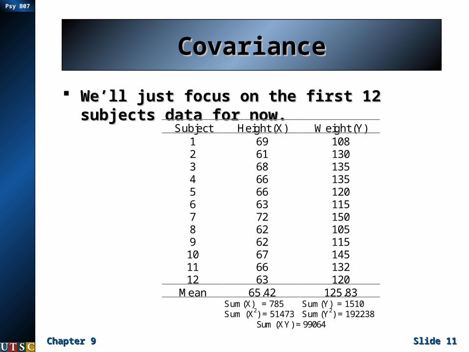
We’ll just focus on the first 12 subjects We’ll just focus on the first 12 subjects data for now.data for now.
Subject Height (X) Weight (Y)1 69 1082 61 1303 68 1354 66 1355 66 1206 63 1157 72 1508 62 1059 62 115
10 67 14511 66 13212 63 120
Mean 65.42 125.83Sum(X) = 785 Sum(Y) = 1510Sum (X2) = 51473 Sum(Y2) = 192238
Sum (XY) = 99064
Chapter 9Chapter 9 Slide Slide 1212
Psy B07
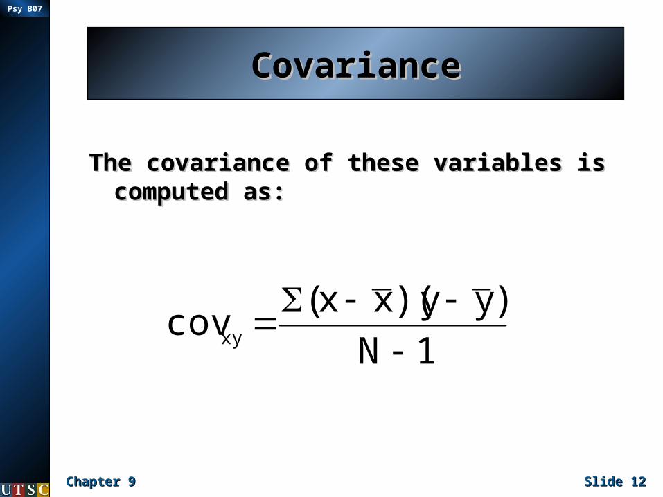
CovarianceCovariance
The covariance of these variables is The covariance of these variables is computed as:computed as:
1N
)yy)(xx(covxy
Chapter 9Chapter 9 Slide Slide 1313
Psy B07
CovarianceCovariance
The covariance formula should look The covariance formula should look familiar to you. If all the Ys were familiar to you. If all the Ys were exchanged for Xs, the covariance exchanged for Xs, the covariance formula would be the variance formula would be the variance formula.formula.
Note what this formula is doing, Note what this formula is doing, however, it is capturing the degree to however, it is capturing the degree to which pairs of points systematically which pairs of points systematically vary around their respective means.vary around their respective means.

Chapter 9Chapter 9 Slide Slide 1414
Psy B07
CovarianceCovariance
If paired X and Y values tend to both be If paired X and Y values tend to both be above or below their means at the same above or below their means at the same time, this will lead to a high positive time, this will lead to a high positive covariance.covariance.
However, if the paired X and Y values tend However, if the paired X and Y values tend to be on opposite sides of their respective to be on opposite sides of their respective means, this will lead to a high negative means, this will lead to a high negative covariance.covariance.
If there is no systematic tendencies of the If there is no systematic tendencies of the sort mentioned above, the covariance will sort mentioned above, the covariance will tend towards zero.tend towards zero.
Chapter 9Chapter 9 Slide Slide 1515
Psy B07
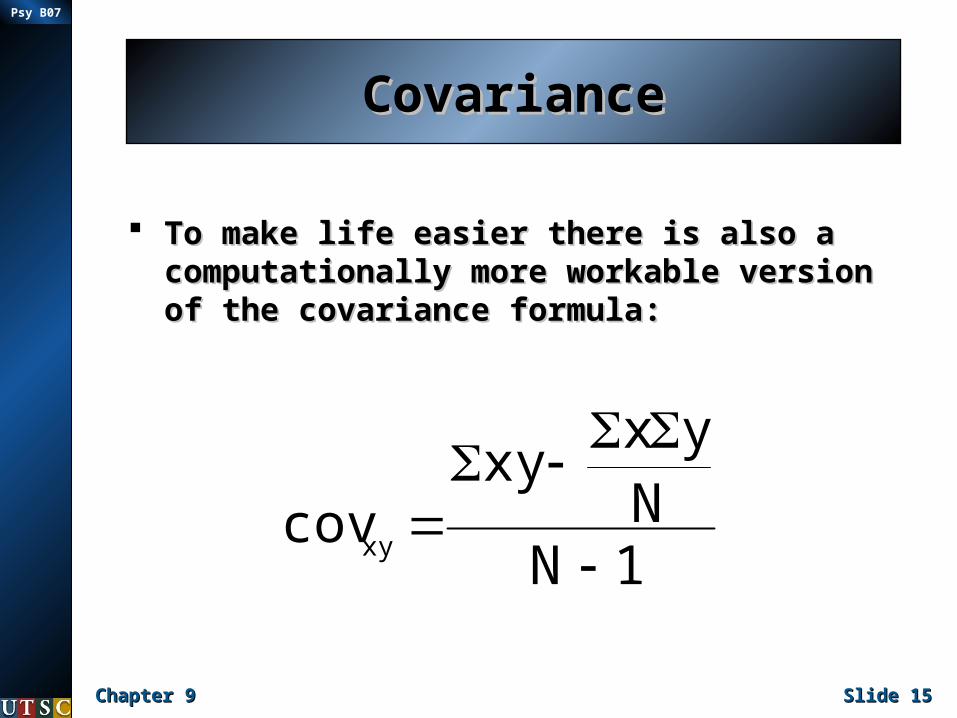
CovarianceCovariance
To make life easier there is also a To make life easier there is also a computationally more workable version computationally more workable version of the covariance formula:of the covariance formula:
1NN
yxxy
covxy
Chapter 9Chapter 9 Slide Slide 1616
Psy B07
CovarianceCovariance
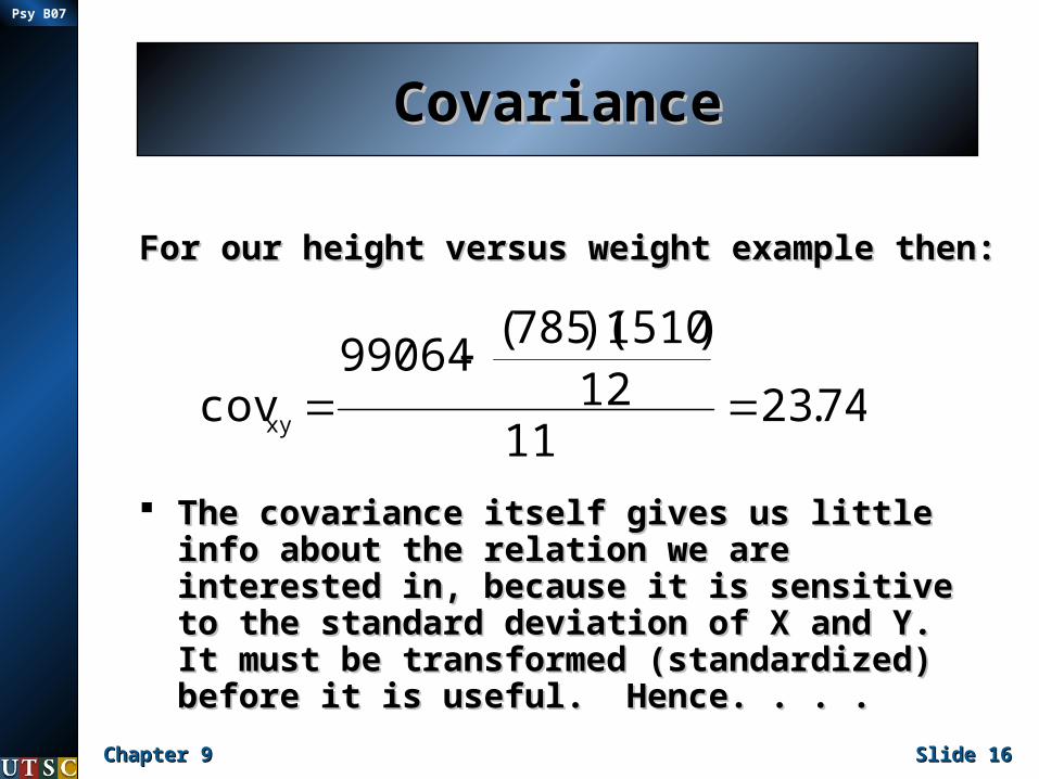
For our height versus weight example then:For our height versus weight example then:
The covariance itself gives us little info The covariance itself gives us little info about the relation we are interested in, about the relation we are interested in, because it is sensitive to the standard because it is sensitive to the standard deviation of X and Y. It must be deviation of X and Y. It must be transformed (standardized) before it is transformed (standardized) before it is useful. Hence. . . .useful. Hence. . . .
74.2311
12)1510)(785(
99064covxy
Chapter 9Chapter 9 Slide Slide 1717
Psy B07
The Pearson Product-The Pearson Product-Moment Correlation Moment Correlation
Coefficient (r)Coefficient (r)
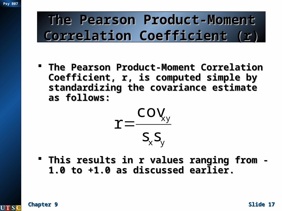
The Pearson Product-Moment Correlation The Pearson Product-Moment Correlation Coefficient, r, is computed simple by Coefficient, r, is computed simple by standardizing the covariance estimate as standardizing the covariance estimate as follows:follows:
This results in r values ranging from -1.0 This results in r values ranging from -1.0 to +1.0 as discussed earlier.to +1.0 as discussed earlier.
yx
xy
ss
covr
Chapter 9Chapter 9 Slide Slide 1818
Psy B07
The Pearson Product-The Pearson Product-Moment Correlation Moment Correlation
Coefficient (r)Coefficient (r)
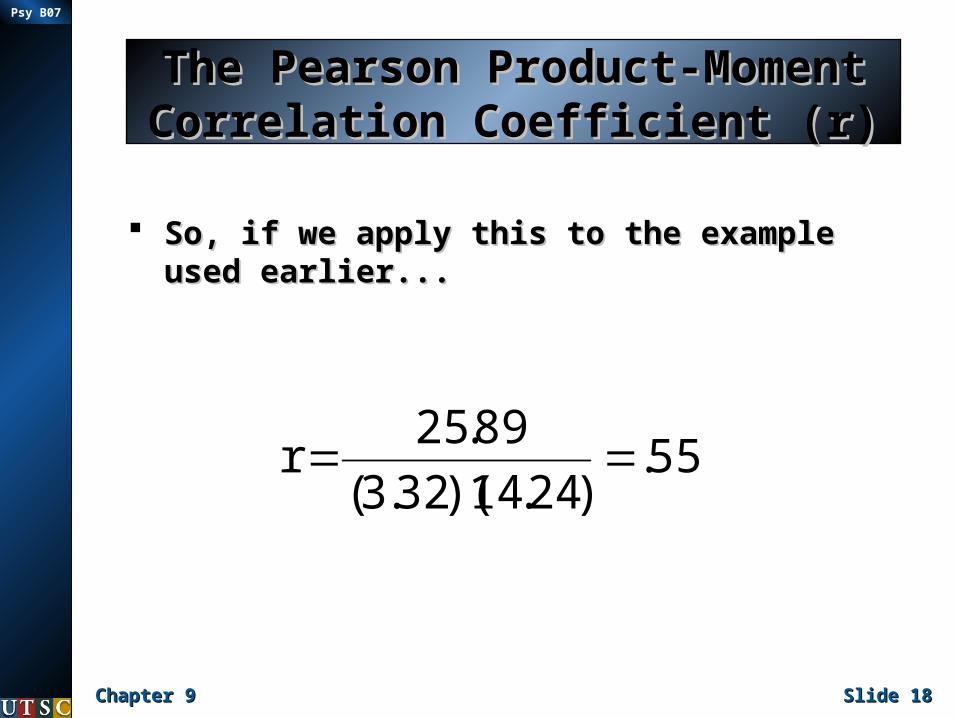
So, if we apply this to the example used So, if we apply this to the example used earlier...earlier...
55.)24.14)(32.3(
89.25r
Chapter 9Chapter 9 Slide Slide 1919
Psy B07
Adjusted rAdjusted r
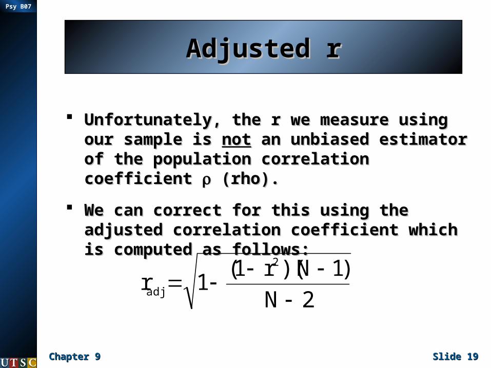
Unfortunately, the r we measure using Unfortunately, the r we measure using our sample is our sample is notnot an unbiased estimator an unbiased estimator of the population correlation coefficient of the population correlation coefficient (rho).(rho).
We can correct for this using the We can correct for this using the adjusted correlation coefficient which is adjusted correlation coefficient which is computed as follows:computed as follows:
2N
)1N)(r1(1r
2
adj
Chapter 9Chapter 9 Slide Slide 2020
Psy B07
Adjusted rAdjusted r
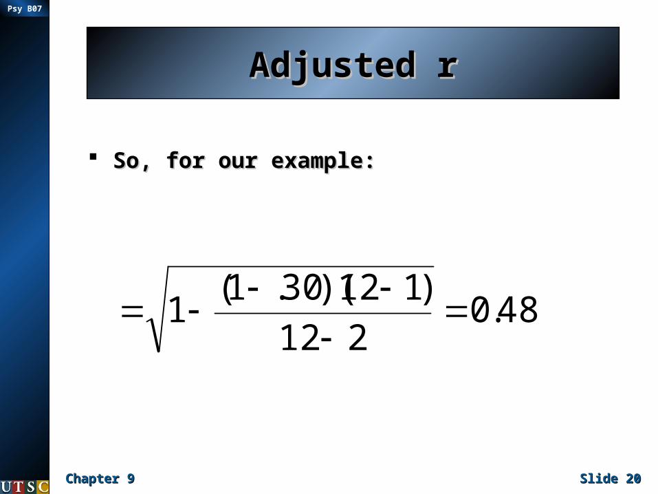
So, for our example:So, for our example:
48.0212
)112)(30.1(1

Chapter 9Chapter 9 Slide Slide 2121
Psy B07
The Regression LineThe Regression Line
Often scatter plots will include a Often scatter plots will include a ‘regression line’ that overlays the points ‘regression line’ that overlays the points in the graph:in the graph:1 1 19 69 108 1 2.5 1.5 7
2 0 18 61 130 1 4 0 83 1 20 68 135 3 5 1 64 0 21 66 135 3 6 0 55 0 26 66 120 1 0 0 86 0 21 63 115 2 4 0 77 1 18 72 150 3 40 0 98 0 19 62 105 1 5 3 79 0 23 62 115 1 8 0 8
10 0 20 67 145 2 5 4 811 0 21 66 132 1 6 1 512 0 20 63 120 2 5 0 713 0 20 67 110 4 4 3 414 0 21 65 100 1 2 0 615 0 19 72 125 1 3 1 716 0 19 61 110 1 2 2 717 0 20 63 110 1 2 1 718 0 21 66 115 1 4 0 719 1 20 68 140 1 3 2 720 0 20 62 113 1 0.5 0 821 1 20 68 190 3 8 22 922 1 20 72 170 2 2 0 823 1 22 67 162 1 6 0 724 0 19 66 140 2 5 5 7
Height vs. Weight
80
100
120
140
160
180
200
220
60 62 64 66 68 70 72 74 76 78
Height (Inches)
Wei
ght
(pou
nds)
Chapter 9Chapter 9 Slide Slide 2222
Psy B07
The Regression LineThe Regression Line
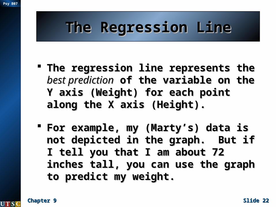
The regression line represents the The regression line represents the best predictionbest prediction of the variable on the of the variable on the Y axis (Weight) for each point along Y axis (Weight) for each point along the X axis (Height).the X axis (Height).
For example, my (Marty’s) data is For example, my (Marty’s) data is not depicted in the graph. But if I not depicted in the graph. But if I tell you that I am about 72 inches tell you that I am about 72 inches tall, you can use the graph to tall, you can use the graph to predict my weight.predict my weight.
Chapter 9Chapter 9 Slide Slide 2323
Psy B07
The Regression LineThe Regression Line
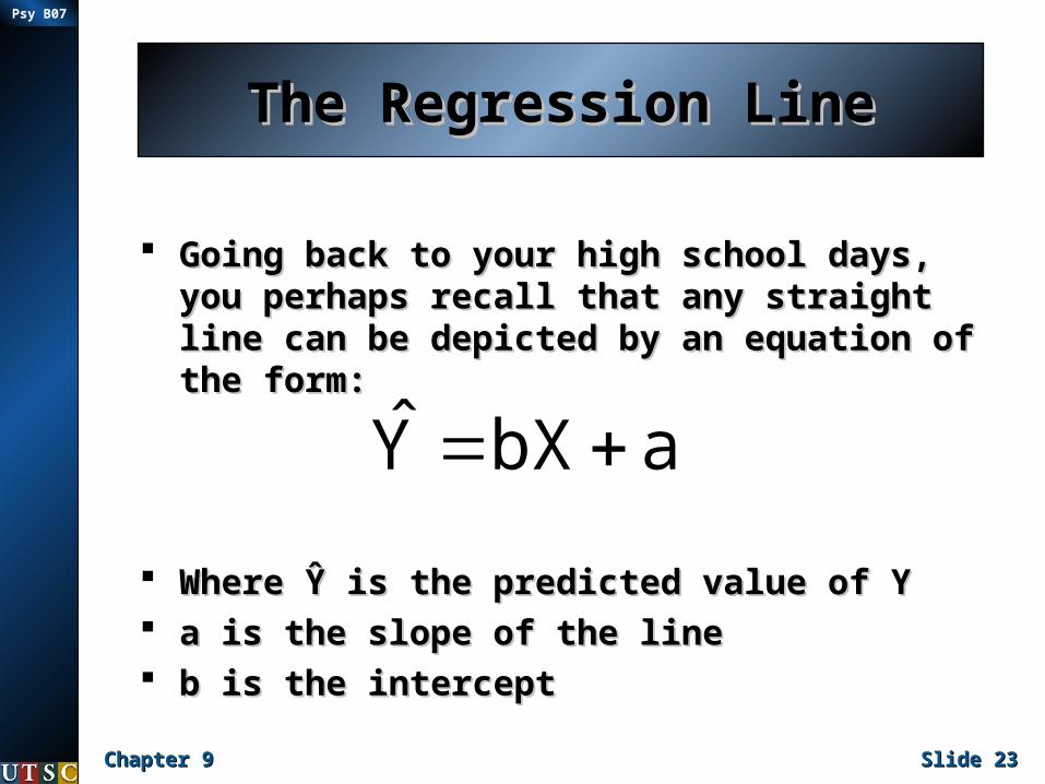
Going back to your high school days, you Going back to your high school days, you perhaps recall that any straight line can perhaps recall that any straight line can be depicted by an equation of the form:be depicted by an equation of the form:
Where Ŷ is the predicted value of YWhere Ŷ is the predicted value of Y a is the slope of the linea is the slope of the line b is the interceptb is the intercept
abXY

Chapter 9Chapter 9 Slide Slide 2424
Psy B07
The Regression LineThe Regression Line
Since the regression line is supposed Since the regression line is supposed to be the line that provides the to be the line that provides the bestbest prediction of Y, given some value of prediction of Y, given some value of X, we need to find values of X, we need to find values of aa & & bb that produce a line that will be the that produce a line that will be the best-fittingbest-fitting linear function (i.e., the linear function (i.e., the predicted values of Y will come as predicted values of Y will come as close as possible to the obtained close as possible to the obtained values of Y).values of Y).
Chapter 9Chapter 9 Slide Slide 2525
Psy B07
The Regression LineThe Regression Line
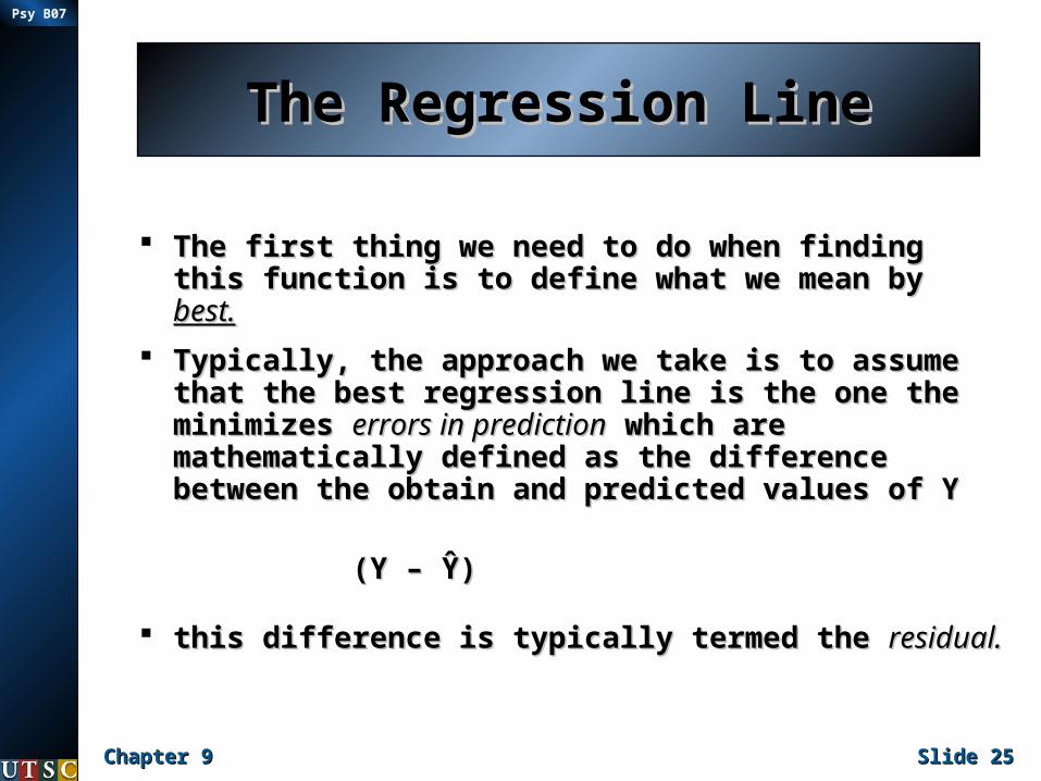
The first thing we need to do when finding this The first thing we need to do when finding this function is to define what we mean by function is to define what we mean by best.best.
Typically, the approach we take is to assume Typically, the approach we take is to assume that the best regression line is the one the that the best regression line is the one the minimizes minimizes errors in predictionerrors in prediction which are which are mathematically defined as the difference mathematically defined as the difference between the obtain and predicted values of Ybetween the obtain and predicted values of Y
(Y – Ŷ)(Y – Ŷ)
this difference is typically termed the this difference is typically termed the residual.residual.

Chapter 9Chapter 9 Slide Slide 2626
Psy B07
The Regression LineThe Regression Line
For reasons similar to those For reasons similar to those involved in computations of involved in computations of variance, we cannot simply variance, we cannot simply minimize minimize ΣΣ(Y-Ŷ) (Y-Ŷ) because that sum because that sum will equal zero for any line passing will equal zero for any line passing through the point (X, Y).through the point (X, Y).
Instead, we must minimize Instead, we must minimize ΣΣ(Y-Ŷ)(Y-Ŷ)22

Chapter 9Chapter 9 Slide Slide 2727
Psy B07
The Regression LineThe Regression Line
At this point, the text book goes through a At this point, the text book goes through a bunch of mathematical stuff showing you bunch of mathematical stuff showing you how to solve for how to solve for aa and and bb by substituting by substituting the equation for a line in for Ŷ in the the equation for a line in for Ŷ in the equation equation ΣΣ(Y-Ŷ)(Y-Ŷ)22, and then minimizing the , and then minimizing the result.result.
You don’t have to know any of that, just You don’t have to know any of that, just the result, which is:the result, which is:
2
x
xy
s
covb XbYa
Chapter 9Chapter 9 Slide Slide 2828
Psy B07
The Regression LineThe Regression Line
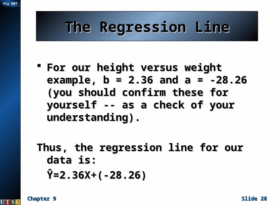
For our height versus weight For our height versus weight example, b = 2.36 and a = -28.26 example, b = 2.36 and a = -28.26 (you should confirm these for (you should confirm these for yourself -- as a check of your yourself -- as a check of your understanding).understanding).
Thus, the regression line for our data Thus, the regression line for our data is:is:
Ŷ=2.36X+(-28.26)Ŷ=2.36X+(-28.26)
Chapter 9Chapter 9 Slide Slide 2929
Psy B07
Residual (or error) Residual (or error) variancevariance
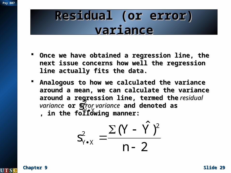
Once we have obtained a regression line, the next Once we have obtained a regression line, the next issue concerns how well the regression line issue concerns how well the regression line actually fits the data.actually fits the data.
Analogous to how we calculated the variance Analogous to how we calculated the variance around a mean, we can calculate the variance around a mean, we can calculate the variance around a regression line, termed thearound a regression line, termed the residual residual variancevariance or or error varianceerror variance and denoted as , in and denoted as , in the following manner:the following manner:
2
XYs
2n
)YY(s
22
XY
Chapter 9Chapter 9 Slide Slide 3030
Psy B07
Residual (or error) Residual (or error) variancevariance
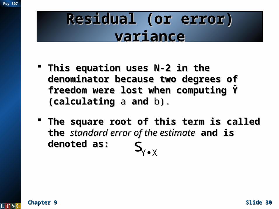
This equation uses N-2 in the This equation uses N-2 in the denominator because two degrees of denominator because two degrees of freedom were lost when computing Ŷ freedom were lost when computing Ŷ (calculating (calculating aa and and b).b).
The square root of this term is called the The square root of this term is called the standard error of the estimatestandard error of the estimate and is and is denoted as:denoted as:
XYs
Chapter 9Chapter 9 Slide Slide 3131
Psy B07
Residual (or error) Residual (or error) variancevariance
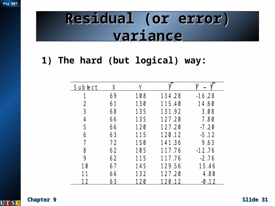
S u b j e c t X Y Y Y – Y1 6 9 1 0 8 1 3 4 . 2 8 - 1 6 . 2 82 6 1 1 3 0 1 1 5 . 4 0 1 4 . 6 03 6 8 1 3 5 1 3 1 . 9 2 3 . 0 84 6 6 1 3 5 1 2 7 . 2 0 7 . 8 05 6 6 1 2 0 1 2 7 . 2 0 - 7 . 2 06 6 3 1 1 5 1 2 0 . 1 2 - 5 . 1 27 7 2 1 5 0 1 4 1 . 3 6 9 . 6 38 6 2 1 0 5 1 1 7 . 7 6 - 1 2 . 7 69 6 2 1 1 5 1 1 7 . 7 6 - 2 . 7 6
1 0 6 7 1 4 5 1 2 9 . 5 6 1 5 . 4 61 1 6 6 1 3 2 1 2 7 . 2 0 4 . 8 01 2 6 3 1 2 0 1 2 0 . 1 2 - 0 . 1 2
1) The hard (but logical) way:

Chapter 9Chapter 9 Slide Slide 3232
Psy B07
Residual (or error) Residual (or error) variancevariance
18.11510
82.11512n
)YY(s
22
XY
Chapter 9Chapter 9 Slide Slide 3333
Psy B07
Residual (or error) Residual (or error) variancevariance
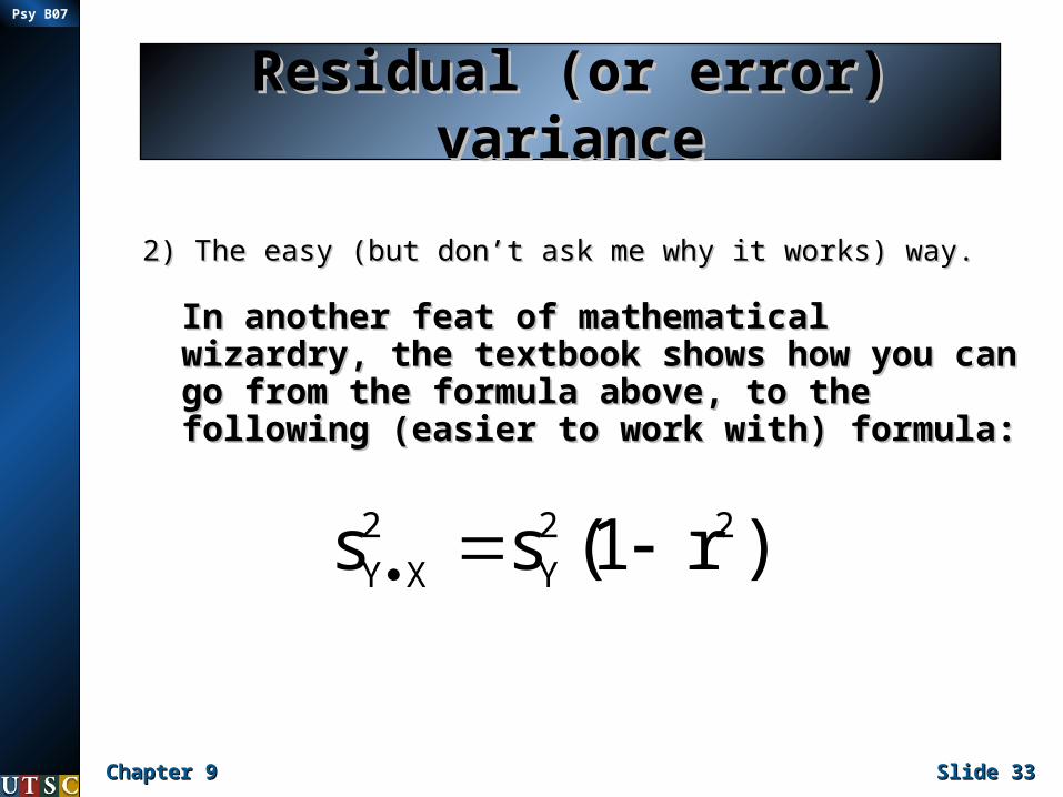
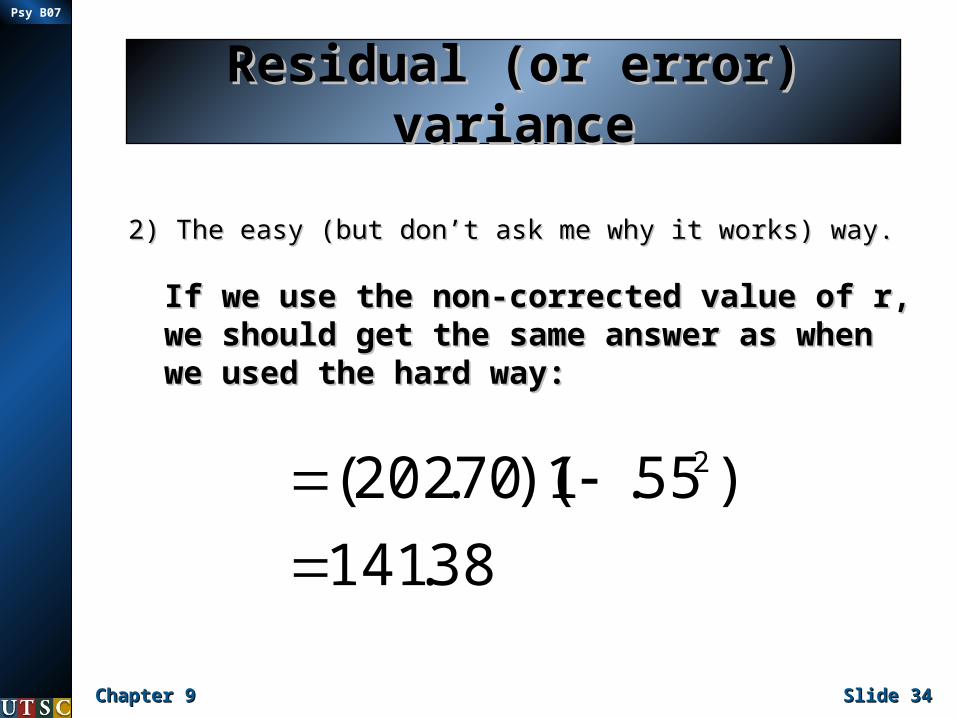
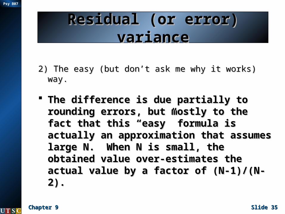
2) The easy (but don’t ask me why it works) way.2) The easy (but don’t ask me why it works) way.
In another feat of mathematical wizardry, In another feat of mathematical wizardry, the textbook shows how you can go from the textbook shows how you can go from the formula above, to the following the formula above, to the following (easier to work with) formula:(easier to work with) formula:
)r1(ss 22
Y
2
XY
Chapter 9Chapter 9 Slide Slide 3434
Psy B07
Residual (or error) Residual (or error) variancevariance
2) The easy (but don’t ask me why it works) way.2) The easy (but don’t ask me why it works) way.
If we use the non-corrected value of r, we If we use the non-corrected value of r, we should get the same answer as when we should get the same answer as when we used the hard way:used the hard way:
38.141
)55.1)(70.202( 2
Chapter 9Chapter 9 Slide Slide 3535
Psy B07
Residual (or error) Residual (or error) variancevariance
2) The easy (but don’t ask me why it works) way.2) The easy (but don’t ask me why it works) way.
The difference is due partially to The difference is due partially to rounding errors, but mostly to the rounding errors, but mostly to the fact that this “easy” formula is fact that this “easy” formula is actually an approximation that actually an approximation that assumes large N. When N is small, assumes large N. When N is small, the obtained value over-estimates the obtained value over-estimates the actual value by a factor of (N-the actual value by a factor of (N-1)/(N-2).1)/(N-2).

Chapter 9Chapter 9 Slide Slide 3636
Psy B07
Hypothesis TestingHypothesis Testing
The text discusses a number of The text discusses a number of hypothesis testing situations relevant hypothesis testing situations relevant to r and b, and gives the test to be to r and b, and gives the test to be performed in each situation.performed in each situation.
I only expect you to know how to test I only expect you to know how to test 1) whether a computed correlation 1) whether a computed correlation coefficient is significantly different coefficient is significantly different from zero, and 2) whether two from zero, and 2) whether two correlations are significantly correlations are significantly different.different.
Chapter 9Chapter 9 Slide Slide 3737
Psy B07
Hypothesis TestingHypothesis Testing
One of the most common reasons One of the most common reasons one examines correlations is to see one examines correlations is to see if two variables are related.if two variables are related.
If the computed correlation If the computed correlation coefficient is significantly different coefficient is significantly different from zero, that suggests that there from zero, that suggests that there is a relation ... the sign of the is a relation ... the sign of the correlation describes exactly what correlation describes exactly what that relation is.that relation is.
Chapter 9Chapter 9 Slide Slide 3838
Psy B07
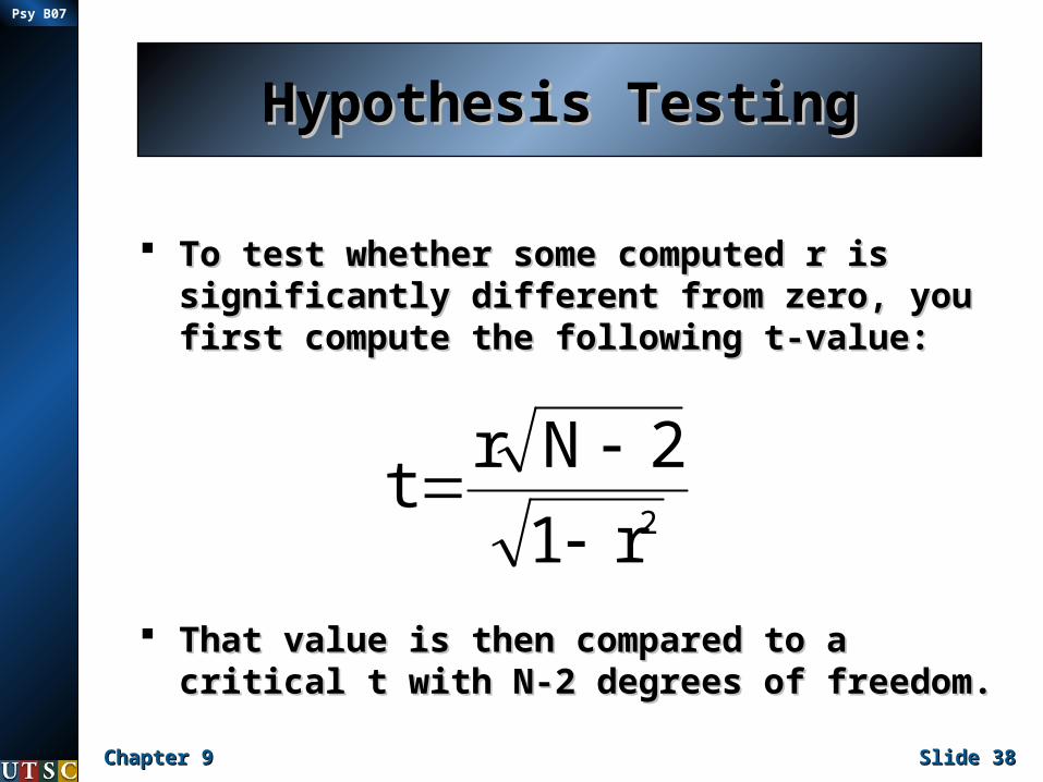
Hypothesis TestingHypothesis Testing
To test whether some computed r is To test whether some computed r is significantly different from zero, you first significantly different from zero, you first compute the following t-value:compute the following t-value:
That value is then compared to a critical t That value is then compared to a critical t with N-2 degrees of freedom.with N-2 degrees of freedom.
2r1
2Nrt
Chapter 9Chapter 9 Slide Slide 3939
Psy B07
Hypothesis TestingHypothesis Testing
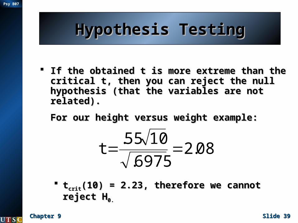
If the obtained t is more extreme than the If the obtained t is more extreme than the critical t, then you can reject the null critical t, then you can reject the null hypothesis (that the variables are not hypothesis (that the variables are not related).related).
For our height versus weight example:For our height versus weight example:
ttcritcrit(10) = 2.23, therefore we cannot (10) = 2.23, therefore we cannot reject Hreject H0.0.
08.26975.
1055.t

Chapter 9Chapter 9 Slide Slide 4040
Psy B07
Hypothesis TestingHypothesis Testing
Testing for a difference between two independent rs Testing for a difference between two independent rs (i.e. does r(i.e. does r11-r-r22=0?) turns out to be a trickier issue, =0?) turns out to be a trickier issue, because the sampling distribution of the difference because the sampling distribution of the difference in two r values is not normally distributed.in two r values is not normally distributed.
Fisher has shown that this problem can be Fisher has shown that this problem can be compensated for by first transforming each of the r compensated for by first transforming each of the r values using the following formula:values using the following formula:
r1
r1log)5.0('r e
Chapter 9Chapter 9 Slide Slide 4141
Psy B07
Hypothesis TestingHypothesis Testing
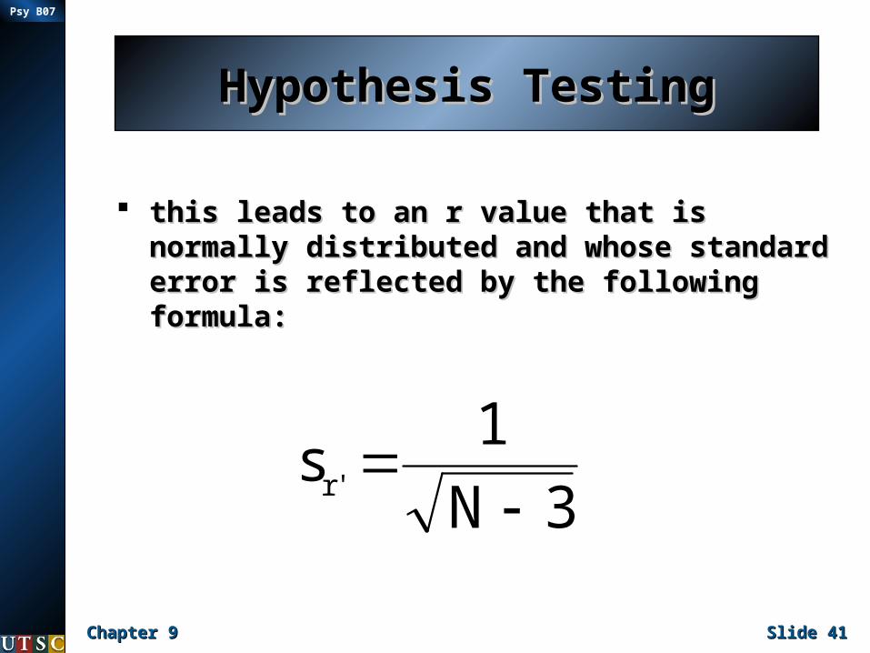
this leads to an r value that is normally this leads to an r value that is normally distributed and whose standard error is distributed and whose standard error is reflected by the following formula:reflected by the following formula:
3N
1s 'r
Chapter 9Chapter 9 Slide Slide 4242
Psy B07
Hypothesis TestingHypothesis Testing
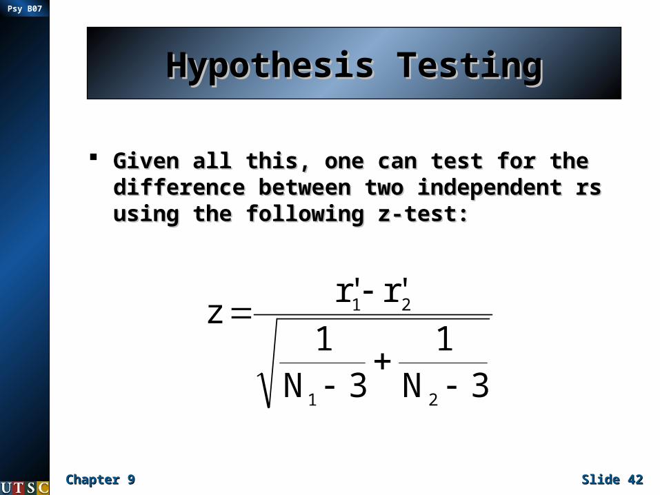
Given all this, one can test for the Given all this, one can test for the difference between two independent rs difference between two independent rs using the following z-test:using the following z-test:
3N1
3N1
'r'rz
21
21
Chapter 9Chapter 9 Slide Slide 4343
Psy B07
Hypothesis TestingHypothesis Testing
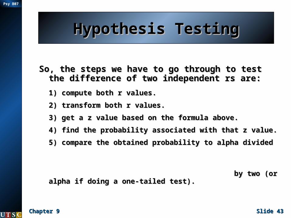
So, the steps we have to go through to test So, the steps we have to go through to test the difference of two independent rs are:the difference of two independent rs are:
1) compute both r values.1) compute both r values.
2) transform both r values.2) transform both r values.
3) get a z value based on the formula above.3) get a z value based on the formula above.
4) find the probability associated with that z value.4) find the probability associated with that z value.
5) compare the obtained probability to alpha 5) compare the obtained probability to alpha divided divided by two (or alpha if by two (or alpha if doing a one-tailed test).doing a one-tailed test).
Chapter 9Chapter 9 Slide Slide 4444
Psy B07
Hypothesis TestingHypothesis Testing
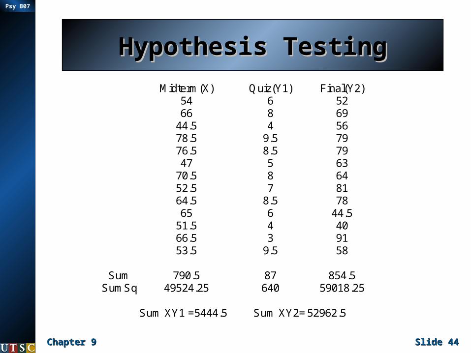
Midterm(X) Quiz(Y1) Final(Y2) 54 6 52 66 8 69 44.5 4 56 78.5 9.5 79 76.5 8.5 79 47 5 63 70.5 8 64 52.5 7 81 64.5 8.5 78 65 6 44.5 51.5 4 40 66.5 3 91 53.5 9.5 58
Sum 790.5 87 854.5 SumSq 49524.25 640 59018.25
Sum XY1 =5444.5 Sum XY2= 52962.5