Pseudo-Rigid-Body Models for Approximating Spatial ...

University of South FloridaScholar Commons

Graduate Theses and Dissertations Graduate School

11-13-2014

Pseudo-Rigid-Body Models for ApproximatingSpatial Compliant Mechanisms of RectangularCross SectionIssa Ailenid RamirezUniversity of South Florida, [email protected]

Follow this and additional works at: https://scholarcommons.usf.edu/etd

Part of the Mechanical Engineering Commons

This Dissertation is brought to you for free and open access by the Graduate School at Scholar Commons. It has been accepted for inclusion inGraduate Theses and Dissertations by an authorized administrator of Scholar Commons. For more information, please [email protected].

Scholar Commons CitationRamirez, Issa Ailenid, "Pseudo-Rigid-Body Models for Approximating Spatial Compliant Mechanisms of Rectangular Cross Section"(2014). Graduate Theses and Dissertations.https://scholarcommons.usf.edu/etd/5562

https://scholarcommons.usf.edu?utm_source=scholarcommons.usf.edu%2Fetd%2F5562&utm_medium=PDF&utm_campaign=PDFCoverPages

https://scholarcommons.usf.edu/etd?utm_source=scholarcommons.usf.edu%2Fetd%2F5562&utm_medium=PDF&utm_campaign=PDFCoverPages

https://scholarcommons.usf.edu/grad?utm_source=scholarcommons.usf.edu%2Fetd%2F5562&utm_medium=PDF&utm_campaign=PDFCoverPages

https://scholarcommons.usf.edu/etd?utm_source=scholarcommons.usf.edu%2Fetd%2F5562&utm_medium=PDF&utm_campaign=PDFCoverPages

http://network.bepress.com/hgg/discipline/293?utm_source=scholarcommons.usf.edu%2Fetd%2F5562&utm_medium=PDF&utm_campaign=PDFCoverPages

mailto:[email protected]

Pseudo-Rigid-Body Models for Approximating Spatial Compliant Mechanisms of Rectangular

Cross Section

by

Issa A. Ramirez

A dissertation submitted in partial fulfillment

of the requirements for the degree of

Doctor of Philosophy

Department of Mechanical Engineering

College of Engineering

University of South Florida

Major Professor: Craig P. Lusk, Ph.D.

Fernando Burgos, Ph.D.

Nathan Crane, Ph.D.

Delcie Durham, Ph.D.

Jing Wang, Ph.D.

Date of Approval:

November 13, 2014

Keywords: Large-deflections, Kinematics, Cantilever beams,

Three-dimensional deflections, Axisymmetric deflections

Copyright © 2014, Issa A. Ramirez

Dedication

To my parents.

Acknowledgments

I would like to express my deep appreciation and gratitude for my advisor, Dr. Craig

Lusk, for his mentorship, patience and guidance thought the completion of this degree. I would

also like to thank my committee members Dr. Burgos, Dr. Crane, Dr. Durham and, Dr. Wang for

their time and helping me to accomplish the doctoral program. I am grateful for the financial

assistance from the McKnight Doctoral Fellowship Program, the Alfred P. Sloan Foundation

Minority Ph.D. program and the National Science Foundation Grant # CMMI-1000138. I wish to

express my gratitude to Mr. Batson for his support and guidance since I started my graduate

studies and throughout all the years at USF. Finally, I would like to thank my mom Dinelia, my

father Isaias, my sister Natasha and my husband Julio, thanks for supporting me and encouraging

me to follow my dreams.

i

Table of Contents

List of Tables ................................................................................................................................. iii

List of Figures ................................................................................................................................ iv

Abstract ......................................................................................................................................... vii

Chapter 1 Introduction .....................................................................................................................1 1.1 Motivation ..................................................................................................................... 1

1.2 Scope ............................................................................................................................. 2 1.3 Goals ............................................................................................................................. 2 1.4 Dissertation Overview .................................................................................................. 2

Literature Review ............................................................................................................5 Chapter 2

2.1 Compliant Mechanisms ................................................................................................ 5

2.1.1 Modeling ........................................................................................................ 6

2.1.1.1 Elliptic Integrals .............................................................................. 7 2.1.1.2 Optimization ................................................................................... 8

2.2 Pseudo-Rigid-Body Model ......................................................................................... 10 2.2.1 End-Force Loading ...................................................................................... 10

2.2.1.1 Stiffness Coefficient...................................................................... 13

2.2.2 End-Moment Loading .................................................................................. 16 2.2.3 Combined Loading: End-Loads and Moments ............................................ 19

Governing Equations of a Flexible Beam .....................................................................22 Chapter 3

3.1 Rotation ....................................................................................................................... 22

3.2 Curvature..................................................................................................................... 25

3.3 Stiffness....................................................................................................................... 27 3.4 Moments Due to Force................................................................................................ 27 3.5 Governing Equations Summary .................................................................................. 29 3.6 Numerical Validation .................................................................................................. 30

3.6.1 Validation of Planar Force in the Y-direction.............................................. 30

3.6.2 Validation of Forces in the XY-plane .......................................................... 30 3.6.3 Validation of Force in Z-direction ............................................................... 32 3.6.4 Validation of Force in the YZ-plane ............................................................ 33 3.6.5 Validation of General XYZ Forces .............................................................. 33

ii

Axisymmetric Pseudo-Rigid-Body Model ....................................................................36 Chapter 4

4.1 Axisymmetric Pseudo-Rigid-Body Model ................................................................. 36 4.2 Force-Loading ............................................................................................................. 39 4.3 Moment Input.............................................................................................................. 43

4.3.1 Out-of-Plane Moment Only (My only) ........................................................ 43 4.3.1.1 Energy Methods Using PRBMs .................................................... 49

4.3.2 Multiple Loading: My and Mz ...................................................................... 52 4.3.2.1 Relative Deflection Error for a Spatial Beam ............................... 54 4.3.2.2 Stiffness for Multiple Moment Loading ....................................... 56

4.4 Conclusion .................................................................................................................. 58

Rectangular Pseudo-Rigid-Body Model with Bending Moment Loads .......................60 Chapter 5

5.1 Governing Equations of a Beam ................................................................................. 60 5.2 Rectangular Pseudo-Rigid-Body Model ..................................................................... 63

5.2.1 Virtual Work ................................................................................................ 65

5.2.2 Virtual Work of the PRBM .......................................................................... 67 5.3 Derivation of PRBM Parameters ................................................................................ 69

5.4 Verification ................................................................................................................. 72 5.5 Approximations of the PRBM Constants ................................................................... 73

5.5.1 Approximation of the Characteristic Radius Factor .................................... 78

5.5.2 Approximation of the Parametric Angle Coefficients ................................. 80 5.5.3 Approximation of the Stiffness Coefficients ............................................... 85

5.6 Summary of PRBM Equations.................................................................................... 89

5.7 Conclusion .................................................................................................................. 90

Conclusions and Recommendations ..............................................................................91 Chapter 6

6.1 Recommendations for Future Work............................................................................ 92

References ......................................................................................................................................93

Appendices .....................................................................................................................................97

Appendix A. Copyright Clearance .................................................................................... 98 Appendix B. Matlab M-file............................................................................................... 99

iii

List of Tables

Table 4.1. Parameters used in the validation of the axisymmetric spatial PRBM. ....................... 43

Table 4.2. PRBM parameters used in the stiffness study. ............................................................ 57

Table 5.1. Limits of the PRBM parameters for different aspect ratios. ........................................ 77

Table 5.2. Approximated values of the characteristic radius factor as a function of the

aspect ratio of the beam. .......................................................................................... 79

Table 5.3. Approximated values of the bending parametric angle coefficient (cθ) as a

function of the aspect ratio of the beam. ................................................................. 82

Table 5.4. Approximated values of cΩa as a function of the aspect ratio of the beam. ................. 84

Table 5.5. Approximated values of the bending stiffness coefficient Kθ and the standard

deviation as a function of the aspect ratio of the beam. .......................................... 86

Table 5.6. Approximated values of the bending stiffness coefficient Kϒ and the standard

deviation as a function of the aspect ratio of the beam. .......................................... 88

Table 5.7. Approximated values of the torsion stiffness coefficient KΣ as a function of the

aspect ratio of the beam. .......................................................................................... 89

iv

List of Figures

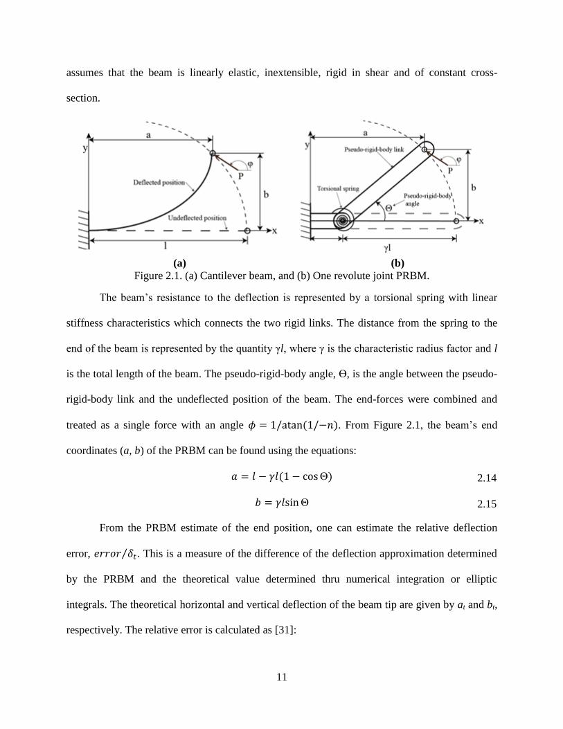
Figure 2.1. (a) Cantilever beam, and (b) One revolute joint PRBM. ............................................ 11

Figure 2.2. 2R PRBM. .................................................................................................................. 15

Figure 2.3. One revolute joint PRBM for end-moment loading. .................................................. 18

Figure 2.4. 3R PRBM. .................................................................................................................. 19

Figure 3.1. Schematic representation of an XZX Euler angle rotation. ........................................ 23

Figure 3.2. Deformed (XYZ) and undeformed (xyz) frames of the cantilever beam. .................. 24

Figure 3.3. Comparison of a spatial cantilever beam results with applied vertical end load

thru numerical integration and FEA. ....................................................................... 31

Figure 3.4. Plot of different values of N with the same force magnitude. .................................... 31

Figure 3.5. Comparison of a spatial cantilever beam results with applied axial end load

thru numerical integration and FEA. ....................................................................... 32

Figure 3.6. Deformation results of a beam in the (a) y-direction and (b) z-direction with

inclined load via integration (line) and FEA (dots). ................................................ 34

Figure 3.7. Nondimensional deformation of beam subjected to the same force at different

N and ζ angles in the (a) y-direction and (b) z-direction. ........................................ 35

Figure 4.1. Axisymmetric PRBM of a cantilever beam................................................................ 38

Figure 4.2. Angles of the applied force in the cantilever beam. ................................................... 39

Figure 4.3. Path results for FEA and spatial PRBM in the (a) y-direction and (b) z-

direction. .................................................................................................................. 42

Figure 4.4. PRBM for an axisymmetric beam with an applied out-of-plane moment.................. 44

Figure 4.5. Nondimensional path results from the 1R PRBM and numerical equations for

a beam with an applied moment in the y-direction, My. .......................................... 45

v

Figure 4.6. Relative deflection error of a cantilever beam versus the tip angle. .......................... 45

Figure 4.7. Exact value of the characteristic radius factor for different tip angles. ...................... 46

Figure 4.8. Exact value of the parametric angle coefficient for various tip angles. ..................... 47

Figure 4.9. Nondimensional path results for the optimized 1R PRBM and numerical

equations for a beam with an applied moment in the y-direction, My. .................... 48

Figure 4.10. Relative deflection error between the theoretical and the governing equations

of a cantilever beam. ............................................................................................... 49

Figure 4.11. Relative deflection error of a cantilever beam versus the input angle of the

applied moment load. .............................................................................................. 50

Figure 4.12. Horizontal versus in-plane deflection for various cases.. ......................................... 53

Figure 4.13. Horizontal versus out-of-plane deflection for varius cases. ..................................... 54

Figure 4.14. Relative deflection error of the optimized 1R PRBM versus the tip slope

angle. ....................................................................................................................... 55

Figure 4.15. Plot of the magnitude of the moment versus the ratio of the in-plane to the

out-of-plane input moment, ε. ................................................................................. 57

Figure 4.16. Percentage error between the applied moment at the end of the beam and the

spring torque. ........................................................................................................... 58

Figure 5.1. Diagram of a cantilever beam with applied moment-loading. ................................... 63

Figure 5.2. PRBM of a cantilever beam with moment loads. ....................................................... 64

Figure 5.3. The frames and the PRBM angles from the fixed to the free-end of the beam. ......... 65

Figure 5.4. Flow chart with the process to derive the PRBM parameters. ................................... 74

Figure 5.5. Angles of the applied moment in the fixed frame. ..................................................... 75

Figure 5.6. Perturbation ratio as a function of the angles of the applied moment 𝜉 and 𝜂

for the 2.5 aspect ratio. ............................................................................................ 77

Figure 5.7. Exact values of the characteristic radius factor, γ, as a function of the tip

angles ϕ and θ and the beam aspect ratio. ................................................................ 78

Figure 5.8. Theoretical and approximated horizontal deflections versus tip angles for

aspect ratio equal to 2. ............................................................................................. 80

vi

Figure 5.9. Exact values of the parametric angle coefficient, cθ, as a function of the tip

angles θ for aspect ratios ranging from 1.25 to 4. .................................................... 81

Figure 5.10. Exact values of the PRB-link parametric angle coefficient, cΩ, as a function

of the tip angles ϕ and θ. .......................................................................................... 83

Figure 5.11. Exact values of the parametric angle coefficient, cΨ, as a function of the tip

angles ϕ and θ. ......................................................................................................... 84

Figure 5.12. Bending stiffness coefficient Kθ as a function of the tip angles ϕ and θ. ................. 85

Figure 5.13. Stiffness parameter Kϒ as a function of the tip angles ϕ and θ. ................................ 87

Figure 5.14. Stiffness parameter KΣ as a function of the tip angles ϕ and θ and the beam

aspect ratio. .............................................................................................................. 88

vii

Abstract

The objective of the dissertation is to develop and describe kinematic models (Pseudo-

Rigid-Body Models) for approximating large-deflection of spatial (3D) cantilever beams that

undergo multiple bending motions thru end-moment loading. Those models enable efficient

design of compliant mechanisms, because they simply and accurately represent the bending and

stiffness of compliant beams.

To accomplish this goal, the approach can be divided into three stages: development of

the governing equations of a flexible cantilever beam, development of a PRBM for axisymmetric

cantilever beams and the development of spatial PRBMs for rectangular cross-section beam with

multiple end moments.

The governing equations of a cantilever beam that undergoes large deflection due to force

and moment loading, contains the curvature, location and rotation of the beam. The results where

validated with Ansys, which showed to have a Pearson’s correlation factor higher than 0.91.

The resulting deflections, curvatures and angles were used to develop a spatial pseudo-

rigid-body model for the cantilever beam. The spatial pseudo-rigid-body model consists of two

links connected thru a spherical joint. For an axisymmetric beam, the PRB parameters are

comparable with existing planar PRBMs. For the rectangular PRBM, the parameters depend on

the aspect ratio of the beam (the ratio of the beam width over the height of the cross-section).

Tables with the parameters as a function of the aspect ratio are included in this work.

1

Chapter 1

Introduction

A compliant mechanism is a device that transforms or transfers motion or energy, which

gains mobility by undergoing elastic deformation on its members. Because they rely on the

deflection of flexible members, they store strain energy in their flexible members. The optimal

compliant mechanism is a compromise between stiffness and flexibility. Because many

applications compliant mechanisms undergo large deformations, linearized beam equations are

no longer valid. Current methods of designing planar compliant mechanisms include elliptic

integrals and the pseudo-rigid-body model.

The pseudo-rigid-body model (PRBM) is a simple method of analyzing systems that

undergo large, nonlinear deflections. It is a simplified form used to model the deflection of

flexible members by using rigid-body joints, links, and springs, that have equivalent force-

deflection characteristics.

1.1 Motivation

Accurate PRBMs that predict the motion of planar beams have been developed. PRBMs

are often used as a first trial in the design phase of different devices and subsequent refinement

can be done using a finite elements program. The PRBM has been used to design medical

devices [1, 2] and MEMS [3-6]. However, spatial compliant mechanisms currently are designed

by trial and error. The motivation of this work is to develop an accurate spatial PRBM to

expedite the design and analysis process for three-dimensional compliant mechanisms.

2

1.2 Scope

Beam analysis can be separated into planar (two-dimensional) beams, axisymmetric and

spatial beams. Analysis of planar PRBMs have been developed in the past with force, moment

and combined loading conditions. Axisymmetric beams are a special case because they are three-

dimensional beams with equal thickness and width. Accurate PRBMs for axisymmetric and

rectangular cross-section spatial beams with moment-loading were developed in this dissertation.

1.3 Goals

The objective of this study is to describe kinematic models (Pseudo-Rigid-Body Models)

for approximating large-deflection of spatial (3D) cantilever beams that undergo in-plane and

out-of-plane bending motions thru end-moment loading. The aims of the present work are:

1. Development of large deflection, non-linear kinematic equations for a cantilever beam,

consisting of curvature, location and rotation equations.

2. Development of pseudo-rigid-body models for an axisymmetric cantilever beam with in-plane

and out-of-plane moment loading:

i. Kinematic parameters: characteristic length and pseudo-rigid-body angle

ii. Stiffness parameters: stiffness coefficients

3. Development of pseudo-rigid-body models for a rectangular cantilever beam with in-plane and

out-of-plane moment loading:

i. Kinematic parameters: characteristic length and pseudo-rigid-body angles

ii. Stiffness parameters: stiffness coefficients

1.4 Dissertation Overview

The motivation of this work is to develop accurate spatial (3D) Pseudo-Rigid-Body

Models (PRBMs) to expedite the design and analysis process of three-dimensional compliant

3

mechanisms. The scope of this study is to describe kinematic models, PRBMs, for approximating

large-deflection of spatial cantilever beams that undergo in-plane and out-of plane bending

motions thru end-moment loading. To accomplish this goal, the approach can be divided into

five stages: development of the governing equations of a flexible cantilever beam, development

of a PRBM for axisymmetric cantilever beams for multiple loads and multiple end-moment

loading, and the development of spatial PRBMs for a rectangular cross-section beam with

multiple end moments.

Chapter 2 presents an overview of the different analysis methods to study large-deflection

of planar and spatial beams, and, analysis methods for compliant mechanisms. Also, an extensive

review of existing pseudo-rigid-body models for cantilever beams is presented.

In Chapter 3, the governing equations of a flexible beam that undergoes large deflection

are derived. The approach used is similar to that found in [7], but the reference frames and

nomenclature selected here facilitates comparison with compliant mechanisms literature. These

equations are validated and used to develop the spatial pseudo-rigid-body models.

Chapter 4 describes the development of a pseudo-rigid-body model for an axisymmetric

multiple force loaded cantilever beam and also a PRBM for an axisymmetric beam with in-plane

and out-of-plane moment loading. The effect of the direction of the loading condition is also

described. The approximated PRB parameters are evaluated to find a PRBM with a relative

deflection error less of 0.5%.

Chapter 5 describes the development of a pseudo-rigid-body model for a rectangular

cantilever beam that undergoes in-plane and out-of-plane moment loading. The kinematic and

stiffness parameters for a beam with rectangular cross-section and bending moments are

described. The perturbation method is used as a measure of the magnitude of the applied out-of-

4

plane moment with respect to the planar moment. With this information, the exact PRBM

parameters for a cantilever beam with multiple end-moments loading were developed. The

PRBM parameters approximations and equations will aid the development of fast and accurate

PRBM’s for spatial cantilever beams.

The dissertation is concluded with a summary and accomplishments of the present work.

Also, recommendations for future work are stated.

5

Chapter 2

Literature Review

This chapter presents an introduction to compliant mechanisms, the advantages and

disadvantages and different design and analysis methods, with emphasis on the pseudo-rigid-

body model.

2.1 Compliant Mechanisms

Compliant mechanisms gain mobility by undergoing elastic deformation of their

members. Because they rely on their deflection of flexible members, energy is stored in form of

strain energy in their flexible links. The optimal compliant mechanism is a balance between

stiffness and flexibility, if too flexible, it will not transmit energy sufficient to do useful work; if

too stiff, it will not deform easily.

The advantages of compliant mechanisms can be divided in two parts: cost reduction and

increased performance [8]. Reduction of the part elements results in reduced assembly time and

simplified manufacturing processes. Part reduction and simplified manufacture processes in

compliant mechanisms are because many of them can be manufactured from an injection-

moldable material or can be constructed in a single piece. Because compliant mechanisms have

fewer movable joints, such as pin and sliding joints, this results in reduced wear and lubrication.

Because of the aforementioned advantages of compliant mechanisms, they may be used for:

Surgical tools and medical devices: compliant mechanisms have been used in medical

devices as forceps-scissors, which is a compliant mechanism end effector that acts as

6

both a forceps and a scissors, and as suturing instruments. Examples of surgical devices

and tools are presented in [1, 9-11].

MEMS devices: compliant mechanisms can be miniaturized and fabricated using

microfabrication techniques such as in MEMS devices. Compliant mechanisms fabricated

at the micro level presents several advantages such as: can be fabricated on plane, require

no assembly, are less complex, have less need for lubrication, have reduced friction and

wear, integrate energy storage elements (like springs) with the other components, and

have higher precision (they have less clearance due to pin joints). Examples of MEMS

devices include an actuator for out-of-plane displacements [12], crash sensors [13], and

compliant stroke amplification mechanisms [14].

Applications in which the mechanism in not easily accessible or for operation in harsh

environments that may adversely affect joints [8].

Aerospace industry: in deployable wings for small unmanned aerial vehicles [15-17] and

flapping wings for micro aerial vehicles [18].

Despite the aforementioned advantages of compliant mechanisms in several applications,

there are disadvantages in the design of compliant mechanisms which include [19]: difficulty of

analysis and design, potential for undesired energy stored in the flexible segments, design for

fatigue is critical, limited rotational ability of flexible links and stress relaxation or creep.

2.1.1 Modeling

Many compliant mechanisms have been designed through trial and error in the past.

These mechanisms are very simple and are not cost efficient for many applications. Knowledge

and synthesis of the compliant members and the interaction with other parts needs to be properly

understood in order to improve and simplify the design of such devices. Because in many

7

applications the flexible members undergo large deformations, linearized beam equations are no

longer valid. Methods for designing planar compliant mechanisms include elliptic integrals [20],

topology optimization [21] and the pseudo-rigid-body model [8].

2.1.1.1 Elliptic Integrals

Elliptic integral solutions can provide rapid feedback in early stages of design to aid the

selection of an appropriate design [22]. The definition of the first and second kind elliptic

integral respectively is:

𝐹(𝜙, 𝑘) = ∫

𝑑𝜃

√1 − 𝑘2𝑠𝑖𝑛2 𝜃

𝜙

0

2.1

𝐸(𝜙, 𝑘) = ∫ √√1 − 𝑘2𝑠𝑖𝑛2𝜃 𝑑𝜃

𝜙

0

2.2

where ϕ is called the magnitude and k is the modulus. Elliptic integral solutions for large

deflection of a cantilever beam with a vertical load at the free end are presented in [20]. The

derivation of a large-deflection solution for a cantilever beam with multiple forces at the free end

is presented in [8]. In the derivation, combined forces are applied to the beam at an angle:

𝜙1 = atan (

1

−𝑛)

2.3

The solution of the nondimensional horizontal and vertical deflection of the beams tip is

[8]:

𝑎

𝑙=

1

𝛼𝜂5/2 {−𝑛𝜂[𝐹(𝑡) − 𝐹(𝛾, 𝑡) + 2(𝐸(𝛾, 𝑡) − 𝐸(𝑡))] + √2𝜂(𝜂 + 𝜆)𝑐𝑜𝑠𝛾} 2.4

𝑏

𝑙=

1

𝛼𝜂5/2 {𝜂[𝐹(𝑡) − 𝐹(𝛾, 𝑡) + 2(𝐸(𝛾, 𝑡) − 𝐸(𝑡))] + 𝑛√2𝜂(𝜂 + 𝜆)𝑐𝑜𝑠𝛾} 2.5

where:

𝛼 =1

√𝜂(𝐹(𝑡) − 𝐹(𝛾, 𝑡)) 2.6

𝛾 = asin√𝜂 − 𝑛

𝜂 + 𝜆 2.7

8

𝑡 = √𝜂 + 𝜆

2𝜂

2.8

𝜂 = √1 + 𝑛2

2.9

𝜆 = 𝜂 cos(𝜃0 − 𝜙1) 2.10

Elliptic integrals solutions for thin beams that undergoes large deflection with multiple

inflection points are presented in [23]. Chen et.al [24] presented the solution of elliptic integrals

and compared them to the PRBM to evaluate its accuracy. Disadvantages of using elliptic

integrals in the design process includes: the derivations are complicated, the solutions can be

found only for relatively simple geometries and loadings, and moreover, this method requires

several simplifying assumptions like linear material properties and inextensible members [8].

2.1.1.2 Optimization

Optimization is the process of finding the conditions that give the maximum or minimum

value of a function, to be able to find the optimum solution depending on a particular set of

design variables [25]. The purpose of optimization is to choose the best design of many

acceptable designs available. The general constrained optimization problem can be stated as

[25]:

Find 𝑋 = {

𝑥1

𝑥2

⋮𝑥𝑛

} which minimizes f(X) 2.11

Subject to the constraints:

𝑔𝑗(𝑋) ≤ 0, 𝑗 = 1,2, … ,𝑚 2.12

lj(𝑋) = 0, 𝑗 = 1,2, … , 𝑝 2.13

where X is an n-dimensional vector called the design vector, f(X) is the objective function, 𝑔𝑗(𝑋)

is known as the inequality term and lj(𝑋) is known as the equality term. The number of

constraints m and p and the number of variables does not have to be related. The objective

9

function is the criterion with respect to which the design is optimized when expressed as a

function of the design problem. It is also called the cost function or energy function. The choice

of the governing function is governed by the nature of the problem.

Sizing, shape and topology optimization addresses different aspects of the design

problem. The definition and design variables characterize the types of optimization such as [26]:

Sizing: in sizing optimization, a typical size of a structure such as the thickness of a beam

and shell elements and material properties such as density are optimized without

changing meshes.

Shape: in shape optimization, the shape of a structure (boundary of design domain such

as the length of a beam and boundary shell) is optimized so that the meshes are varied as

the design changes. The shape optimization problem may have multiple solutions,

because the domain in which to look for the final design is not determined yet.

Topology: the topology of a structure is optimized so that the shape and connectivity of

design domain are altered. Topology optimization is the most general form of structural

optimization.

The most popular design method is topology optimization. Sigmund et al.[27] presented

an energy-based topology optimization. Lee et al.[28] presented a strain-based topology

optimization method that avoids localized high strain in compliant joints of the compliant

mechanism. Pedersen et al.[29] presented the design of a large displacement compliant

mechanism. Compliant mechanisms design through topology optimization includes a conceptual

design of a wing-flapping mechanism [30].

10

2.2 Pseudo-Rigid-Body Model

It was observed that in cantilever beams undergoing large deflections, the path of the

beam end is nearly circular, with a center of curvature at some point on the undeflected part of

the beam. This observation served as the catalyst that leads to the development of the pseudo-

rigid-body model, which allows the motion of the end of the cantilever beam to be accurately

predicted [8].

The pseudo-rigid-body model (PRBM) is a simple method of analyzing systems that

undergo large, nonlinear deflections. It is a simplified form used to model the deflection of

flexible members by using rigid-body joints that have the equivalent force-deflection

characteristics. The PRBM predicts the deflection path and force-deflection relationship of

flexible segments, modeling them as rigid links attached at the pin joints. Springs are added to

predict the force-displacement relationship of the flexible members.

Existing PRBMs differ in the number and the location of the links and joints. Also, the

pseudo-rigid-body parameters depend on the loading conditions: end-forces, end-moments and

combined loading. Planar PRBMs that predict the location of the free-end of the beam for

different loading conditions are presented in the following section.

2.2.1 End-Force Loading

Because the path of the free end of a cantilever beam end is nearly circular, with a center

of curvature at some point on the undeflected part of the beam, it can be modeled as two links

connected by a pivot. The first model of a PRBM for a cantilever beam consists of 2 rigid-body

links connected through a revolute (1R) joint [31], as shown in Figure 2.1. The approximate

equations for nonlinear, large deflection cantilever beams with end-forces and no moments,

11

assumes that the beam is linearly elastic, inextensible, rigid in shear and of constant cross-

section.

(a) (b)

Figure 2.1. (a) Cantilever beam, and (b) One revolute joint PRBM.

The beam’s resistance to the deflection is represented by a torsional spring with linear

stiffness characteristics which connects the two rigid links. The distance from the spring to the

end of the beam is represented by the quantity γl, where γ is the characteristic radius factor and l

is the total length of the beam. The pseudo-rigid-body angle, ϴ, is the angle between the pseudo-

rigid-body link and the undeflected position of the beam. The end-forces were combined and

treated as a single force with an angle 𝜙 = 1/atan (1/−𝑛). From Figure 2.1, the beam’s end

coordinates (a, b) of the PRBM can be found using the equations:

𝑎 = 𝑙 − 𝛾𝑙(1 − cos Θ) 2.14

𝑏 = 𝛾𝑙sin Θ 2.15

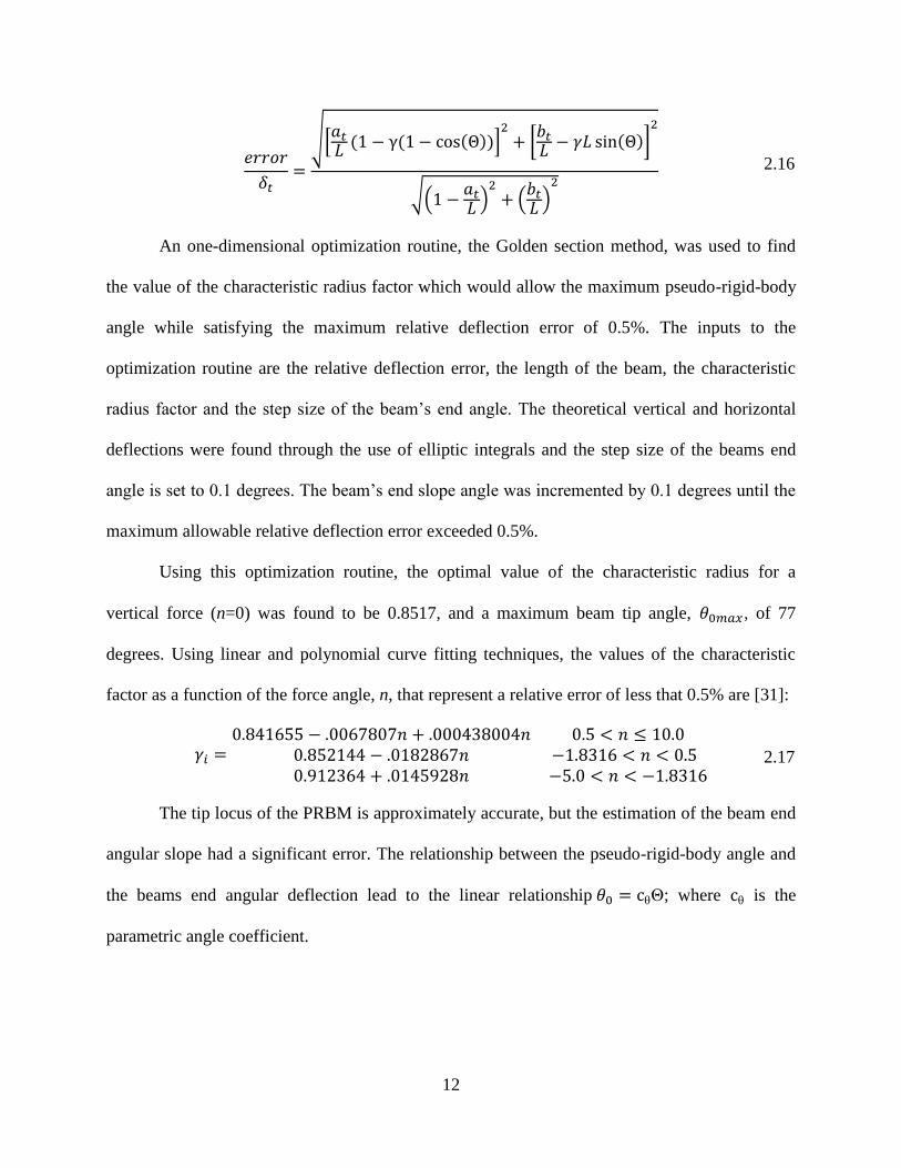
From the PRBM estimate of the end position, one can estimate the relative deflection

error, 𝑒𝑟𝑟𝑜𝑟 𝛿𝑡⁄ . This is a measure of the difference of the deflection approximation determined

by the PRBM and the theoretical value determined thru numerical integration or elliptic

integrals. The theoretical horizontal and vertical deflection of the beam tip are given by at and bt,

respectively. The relative error is calculated as [31]:

12

𝑒𝑟𝑟𝑜𝑟

𝛿𝑡=

√[𝑎𝑡

𝐿 (1 − γ(1 − cos(Θ))]2

+ [𝑏𝑡

𝐿 − 𝛾𝐿 sin(Θ)]2

√(1 −𝑎𝑡

𝐿 )2

+ (𝑏𝑡

𝐿 )2

2.16

An one-dimensional optimization routine, the Golden section method, was used to find

the value of the characteristic radius factor which would allow the maximum pseudo-rigid-body

angle while satisfying the maximum relative deflection error of 0.5%. The inputs to the

optimization routine are the relative deflection error, the length of the beam, the characteristic

radius factor and the step size of the beam’s end angle. The theoretical vertical and horizontal

deflections were found through the use of elliptic integrals and the step size of the beams end

angle is set to 0.1 degrees. The beam’s end slope angle was incremented by 0.1 degrees until the

maximum allowable relative deflection error exceeded 0.5%.

Using this optimization routine, the optimal value of the characteristic radius for a

vertical force (n=0) was found to be 0.8517, and a maximum beam tip angle, 𝜃0𝑚𝑎𝑥, of 77

degrees. Using linear and polynomial curve fitting techniques, the values of the characteristic

factor as a function of the force angle, n, that represent a relative error of less that 0.5% are [31]:

𝛾𝑖 =0.841655 − .0067807𝑛 + .000438004𝑛 0.5 < 𝑛 ≤ 10.0

0.852144 − .0182867𝑛 −1.8316 < 𝑛 < 0.5 0.912364 + .0145928𝑛 −5.0 < 𝑛 < −1.8316

2.17

The tip locus of the PRBM is approximately accurate, but the estimation of the beam end

angular slope had a significant error. The relationship between the pseudo-rigid-body angle and

the beams end angular deflection lead to the linear relationship 𝜃0 = cθΘ; where cθ is the

parametric angle coefficient.

13

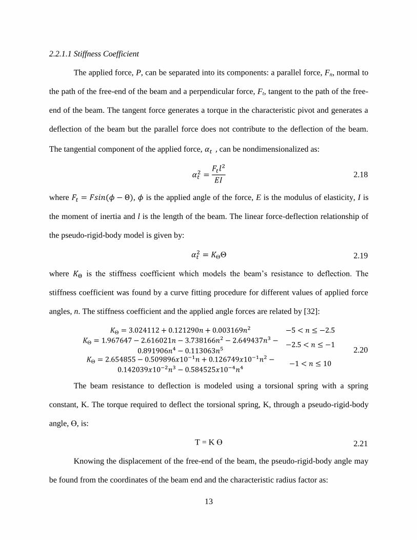
2.2.1.1 Stiffness Coefficient

The applied force, P, can be separated into its components: a parallel force, Fn, normal to

the path of the free-end of the beam and a perpendicular force, Ft, tangent to the path of the free-

end of the beam. The tangent force generates a torque in the characteristic pivot and generates a

deflection of the beam but the parallel force does not contribute to the deflection of the beam.

The tangential component of the applied force, 𝛼𝑡 , can be nondimensionalized as:

𝛼𝑡2 =

𝐹𝑡𝑙2

𝐸𝐼 2.18

where 𝐹𝑡 = 𝐹𝑠𝑖𝑛(𝜙 − Θ), 𝜙 is the applied angle of the force, E is the modulus of elasticity, I is

the moment of inertia and l is the length of the beam. The linear force-deflection relationship of

the pseudo-rigid-body model is given by:

𝛼𝑡2 = 𝐾ΘΘ 2.19

where 𝐾Θ is the stiffness coefficient which models the beam’s resistance to deflection. The

stiffness coefficient was found by a curve fitting procedure for different values of applied force

angles, n. The stiffness coefficient and the applied angle forces are related by [32]:

𝐾Θ = 3.024112 + 0.121290𝑛 + 0.003169𝑛2 −5 < 𝑛 ≤ −2.5

𝐾Θ = 1.967647 − 2.616021𝑛 − 3.738166𝑛2 − 2.649437𝑛3 −

0.891906𝑛4 − 0.113063𝑛5−2.5 < 𝑛 ≤ −1

𝐾Θ = 2.654855 − 0.509896𝑥10−1𝑛 + 0.126749𝑥10−1𝑛2 −

0.142039𝑥10−2𝑛3 − 0.584525𝑥10−4𝑛4−1 < 𝑛 ≤ 10

2.20

The beam resistance to deflection is modeled using a torsional spring with a spring

constant, K. The torque required to deflect the torsional spring, K, through a pseudo-rigid-body

angle, ϴ, is:

T = K ϴ 2.21

Knowing the displacement of the free-end of the beam, the pseudo-rigid-body angle may

be found from the coordinates of the beam end and the characteristic radius factor as:

14

Θ = atanb

a − l(1 − γ) 2.22

The torsional spring stiffness, K, can be found as:

K = 𝛾𝐾ΘEI

l⁄ 2.23

Pauly et al. [33] modified Howell’s 1R PRBM optimization routine for end-loaded

cantilever beams. A change in the beam’s end slope, 𝜃0, equal to 0.1 degrees was adequate for

loads in the range of 45≤ 𝜙. In order to ensure that the relative deflection error is less than 0.5%,

in forces that are nearly axial, tensile end loads, were modified to have the change of the end

angular deflection, ∆𝜃0, equal to 1 x 10-5

degrees. The Golden section technique was used to

solve the optimization problem with values of the change of the end angular deflection of 1 x

10-5

degrees and a relative deflection error of 0.5%. The pseudo-rigid-body model parameter as a

function of the load parameter (n) was modified to accommodate the changes [33]:

𝛾 =

0.855651 − .016438𝑛 −4.0 < 𝑛 ≤ −1.50.852138 − .018615𝑛 −1.5 < 𝑛 ≤ 0.5

0.851892 − 0.020805𝑛 + 0.005867𝑛2 − 0.000895𝑛3 + 0.000069𝑛4 − 0.000002𝑛5 0.5 < 𝑛 ≤ 10

2.24

Dado et al. [34] presented a variable parametric pseudo-rigid-body model for large

deflection beams with end-loads based on the 1R PRBM. The model finds correlation equations

that relate the stiffness and the load in terms of the characteristic radius and the pseudo-rigid-

body angle through regression analysis. A disadvantage of this model is the need of an

interactive procedure to find the values of the beam’s end (a and b).

Feng et al. [35] presented a two revolute joint (2R) PRBM that can simulate the tip locus

and the tip deflection angle, and showed that the 2R model has superior kinematics than the 1R

model. The 2R PRBM consists of 3 rigid links connected thru 2 revolute joints and 2 torsion

springs as shown in Figure 2.2.

15

Figure 2.2. 2R PRBM.

The slope angle for the 2R PRBM is equal to 𝜃0 = Θ = Θ1 + Θ2, as shown in Figure 2.2.

The characteristic radius factor satisfies the equation:

𝛾0 + 𝛾1 + 𝛾2 = 1 2.25

A two-dimensional search process is used to find the optimal characteristic radius factor.

The inputs to the optimization are the length of the beam, a set of three characteristic radius

factors, a step size of the beam’s end angle of 0.02 and a maximum angle error of 1%. The

relationship between the characteristic radius and the force angle is given by [35]:

𝛾𝑖(𝑖 = 1,2,3) =

0.08,0.52,0.40 0 < 𝜙 ≤ 63. 4𝑜

0.10,0.54,0.36 63. 4𝑜 < 𝜙 ≤ 116.6𝑜, 153.4𝑜 < 𝜙 < 180𝑜

0.12,0.56,0.32 116.6𝑜 < 𝜙 ≤ 153. 4𝑜 2.26

Using a linear regression process, the approximated values of the spring stiffness

coefficients (𝐾Θi) are found. The relation between the spring stiffness coefficients and the

applied force angle is given by [35]:

𝐾Θ1 = −1.4584𝜙2 + 4.5794𝜙 − 0.0421

𝐾Θ2 = −0.6133𝜙2 + 1.9403𝜙 − 0.0982 2.27

For a vertical force (n=0), the results represents an error smaller than 1% with a

parametric maximum angle 𝜃0𝑚𝑎𝑥 = 83.5 degrees. Because the error between the slope angle of

16

the 2R PRBM (Θ), and the link tip deflection (𝜃0) is less than 1%, there is no need for a

parametric angle coefficient (𝑐𝜃) and the link tip deflection angle can be equal to the slope of the

2R PRBM (𝜃0 = Θ).

The advantages of Feng’s 2R PRBM is that there is no need of a parametric coefficient

because it simulates the tip locus and the tip angle, because the error between the beam’s tip

deflection and the slope of the 2R PRBM is less than 1%. Another advantage is that the

maximum angular slope was increased from 77 degrees in the 1R PRBM to 88.5 degrees in the

2R PRBM. A disadvantage of the model is that it only takes in consideration end-beam loading

and there are no cases for input moments.

2.2.2 End-Moment Loading

Compliant mechanisms undergo large deflections which introduces geometric

nonlinearities. The major difference between small and large deflection analysis lies in the

assumptions made to solve the Bernoulli-Euler equations [8]. The Bernoulli–Euler theory is a

simplified theory for the calculation of the deflection of beams. The basic assumptions of the

theory are [36]: 1) the beam is elastic and isotropic, 2) the beam deformation is dominated by

bending, and, 3) the beam is long and slender with a constant cross section along the axis.

The Bernoulli-Euler equation of a cantilever beam subjected to a moment end-load states

that the bending moment is proportional to the beam’s curvature, such as:

𝑀 = 𝐸𝐼𝑑𝜃

𝑑𝑠 2.28

where M is the applied moment, E is the Young’s modulus, I is the moment of inertia and,

𝑑𝜃 𝑑𝑠⁄ is the rate of angular deflection along the beam, also known as curvature. For a planar

beam with an applied moment at the free end, M, the internal moment is constant along the

beam. The angular deflection of the beams end, 𝜃0, is found by separating variables,

17

∫ 𝑑𝜃𝜃0

0

= ∫𝑀

𝐸𝐼𝑑𝑠

𝐿

0

2.29

And integrating, the angular deflection of the beam is:

𝜃0 =𝑀𝐿

𝐸𝐼 2.30

where the angular deflection of the beam’s end, 𝜃0, is in radians. The rate of vertical deflection

along the beam’s length is 𝑑𝑦 𝑑𝑠⁄ = sin 𝜃. The vertical deflection, b, can be found by the chain

rule of differentiation, and substituting, such as:

𝑀

𝐸𝐼=

𝑑𝜃

𝑑𝑠=

𝑑𝜃

𝑑𝑦

𝑑𝑦

𝑑𝑠=

𝑑𝜃

𝑑𝑦sin 𝜃 2.31

Separating variables,

∫ 𝑑𝑦𝑏

0

=𝐸𝐼

𝑀∫ sin 𝜃 𝑑𝜃

𝜃0

0

2.32

And integrating, the vertical deflection of the beam is:

𝑏 =𝐸𝐼

𝑀(1 − cos 𝜃0) 2.33

Substituting into Equation 2.30:

𝑏 =𝑙 − 𝑙 𝑐𝑜𝑠 𝜃0

𝜃0 2.34

In the same manner, the horizontal deflection of the free end of the beam can be found.

The rate of horizontal deflection along the beam’s length is 𝑑𝑥 𝑑𝑠⁄ = cos 𝜃. The horizontal

deflection of the free end of the beam, a, can be found by the chain rule of differentiation,

substituting, and separating into variables such as:

∫ 𝑑𝑥𝑎

0

=𝐸𝐼

𝑀∫ cos 𝜃 𝑑𝜃

𝜃0

0

2.35

Integrating, the horizontal deflection of the beam is:

18

𝑎 =𝐸𝐼

𝑀sin 𝜃0 2.36

Substituting in Equation 2.30:

𝑎 =l sin 𝜃0

𝜃0 2.37

The nondimensional large-deflection equations of a cantilever beam with a moment load

can be found [8]:

𝑎

𝑙=

sin (M0LEI )

M0lEI

2.38

𝑏

𝑙=

EI

M0l [1 − cos (θ0)] 2.39

where a and b are the horizontal and vertical coordinates of the free-end of the beam, M0 is the

applied moment, I is the moment of inertia, l is the length of the beam and E is the modulus of

elasticity.

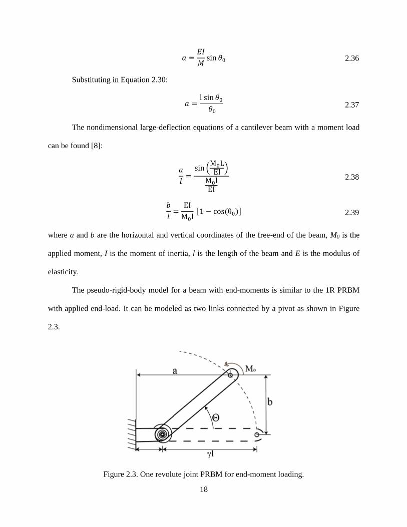
The pseudo-rigid-body model for a beam with end-moments is similar to the 1R PRBM

with applied end-load. It can be modeled as two links connected by a pivot as shown in Figure

2.3.

Figure 2.3. One revolute joint PRBM for end-moment loading.

19

The optimal value of the characteristic radius for an applied moment that gives a relative

deflection error less than 0.5% was found to be 0.7346, the maximum beam tip slope angle,

𝜃0𝑚𝑎𝑥, of 124.4 degrees and the parametric angle coefficient, 𝑐θ, was found to be 1.5164. The

spring constant for the case of an end-moment is given by [8]:

𝐾 = 𝑐θ

EI

L 2.40

2.2.3 Combined Loading: End-Loads and Moments

Su et al. [37] developed a 3 revolute (3R) PRBM for a planar, initially straight beam

which consists of 4 rigid links connected thru three revolute joints as shown in Figure 2.4. A

three-dimensional search routine was used to find the optimal set of the characteristic radius and

the spring stiffness. This model can be used to for different types of loading conditions: end-

moment only, end-force and combined loading.

Figure 2.4. 3R PRBM.

20

For a pure moment load, the maximum error of the tip deflection was found to be 2.3% of

the beams length for beam tip slopes less than 270 degrees. The approximated values of the

spring stiffness computed are [37]:

𝑘1 = 3.51933 EIl⁄ 𝑘2 = 2.78518 EI

l⁄ 𝑘3 = 2.79756 EIl⁄ 2.41

The effect of the force angle, 𝜙, was neglected in finding the optimized PRBM because

the spring stiffness was only correlated slightly to the direction of the force. The error was found

to be minimized with the 3R PRBM. With a pure vertical force, 𝜙 = 90 degrees, the model has

an error of 1.2% when 𝜃0 = 90 degrees compared to 3.6% for the 1R PRBM. The approximated

values of the spring stiffness computed are [37]:

𝑘1 = 3.71591 EIl⁄ 𝑘2 = 2.87128 EI

l⁄ 𝑘3 = 2.26417 EIl⁄ 2.42

For a straight cantilever beam subjected to an end-force, P, and an end-moment, M, the

nondimensional force index, α, and load ratio, κ, equations are:

α =Pl2

2EI β =

Ml

EI κ =

β2

4α 2.43

The effect of the angle of the force is neglected because it is shown that the spring

stiffness is only slightly correlated to the direction of the applied force. The maximum deflection

error is 2.2% of the beam’s length. The characteristic radius for combined loading with a

nondimentional load ratio, κ, between 0-25 with vertical loads are:

𝛾0 = 0.1 𝛾1 = 0.35 𝛾2 = 0.40 𝛾3 = 0.15 2.44

The spring stiffnesses for combined loading with a nondimentional load ratio, κ, between

0-25 with vertical loads are:

𝑘1 = 3.51 EIl⁄ 𝑘2 = 2.99 EI

l⁄ 𝑘3 = 2.58 EIl⁄ 2.45

21

The benefits of the 3R PRBM are [25, 37, 38]: load independence, high accuracy for

large deflection beams and explicit kinematic and static constraint equations. Disadvantages of

the 3R PRBM include [37]: assumed no inflection point in the beam and the force angle, 𝜙, is

limited to 9 − 171 degrees to have an accurate approximation.

The earlier section presented the literature review of various PRBMs for different types

of loading. To develop a spatial pseudo-rigid-body model, the kinematic equations of the beam

are derived. Chapter 3 presents the governing equations of a flexible beam that undergoes large

deflection.

22

Chapter 3

Governing Equations of a Flexible Beam1

The governing equations of a flexible beam are derived in this chapter. The approach

used is similar to the one presented in [7]. However, the reference frames and nomenclature

selected for this derivation facilitates the analysis and comparison with compliant mechanisms

literature. The derived equations will be validated using a finite element analysis program.

The equations that describe the large deflection of a spatial cantilever beam are derived in

four steps. First, the rotation angles describing the bending and twisting of the beam are given.

Next, equations for the curvature of the beam are derived. Thirdly, the stiffness properties of the

beam are described. Fourthly, the internal moments due to applied forces are described. Finally,

the equations are summarized in a form suitable for numerical integration.

3.1 Rotation

The equations describing the deformation of the beam from its unstressed coordinates,

xyz, to its deformed coordinates, x’y’z’, may be found using three rotations matrices. The first

two rotations describe the change in the orientation of a segment, ds, of the neutral axis. The

third rotation describes the twisting of the beam about the deflected orientation of the neutral

axis.

_________________________ 1Portions of this chapter were previously published in [44]. Permission is included in Appendix A.

23

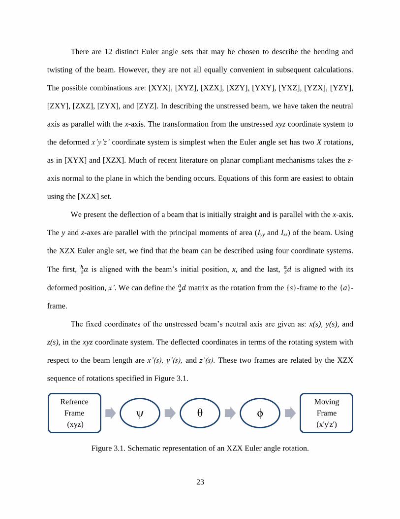
There are 12 distinct Euler angle sets that may be chosen to describe the bending and

twisting of the beam. However, they are not all equally convenient in subsequent calculations.

The possible combinations are: [XYX], [XYZ], [XZX], [XZY], [YXY], [YXZ], [YZX], [YZY],

[ZXY], [ZXZ], [ZYX], and [ZYZ]. In describing the unstressed beam, we have taken the neutral

axis as parallel with the x-axis. The transformation from the unstressed xyz coordinate system to

the deformed x’y’z’ coordinate system is simplest when the Euler angle set has two X rotations,

as in [XYX] and [XZX]. Much of recent literature on planar compliant mechanisms takes the z-

axis normal to the plane in which the bending occurs. Equations of this form are easiest to obtain

using the [XZX] set.

We present the deflection of a beam that is initially straight and is parallel with the x-axis.

The y and z-axes are parallel with the principal moments of area (Iyy and Izz) of the beam. Using

the XZX Euler angle set, we find that the beam can be described using four coordinate systems.

The first, 𝑎𝑠ℎ is aligned with the beam’s initial position, x, and the last, 𝑑𝑠

𝑎 is aligned with its

deformed position, x’. We can define the 𝑑𝑠𝑎 matrix as the rotation from the {s}-frame to the {a}-

frame.

The fixed coordinates of the unstressed beam’s neutral axis are given as: x(s), y(s), and

z(s), in the xyz coordinate system. The deflected coordinates in terms of the rotating system with

respect to the beam length are x’(s), y’(s), and z’(s). These two frames are related by the XZX

sequence of rotations specified in Figure 3.1.

Figure 3.1. Schematic representation of an XZX Euler angle rotation.

Refrence

Frame

(xyz)

ψ θ ϕ Moving

Frame

(x'y'z')

24

It is also useful to define another coordinate system at the free-end of the deflected

cantilever as the XYZ frame: X(s), Y(s), and Z(s) as shown in Figure 3.2.

Figure 3.2. Deformed (XYZ) and undeformed (xyz) frames of the cantilever beam.

For an initially straight beam, we can choose to align the neutral axis of the unstressed

beam with the x-axis in the xyz coordinate system. Thus:

x(s) = s 3.1

y(s) = 0 3.2

z(s) = 0 3.3

The coordinate frame 𝑑𝑠𝑎 , describes the orientation of the neutral axis and the beams twist

about the neutral axis. The transformation coordinates from the deformed ( 𝑑𝑠𝑎 ) to the undeformed

( 𝑎𝑠ℎ ) frame is given by:

𝑑𝑠𝑎 = 𝑅𝑝

𝑎 (𝜙) 𝑅𝑞𝑝 (θ) 𝑅ℎ

𝑞 (𝜓) 𝑎𝑠ℎ = 𝑅𝑝

𝑎 (𝜙) 𝑅𝑞𝑝 (θ) 𝑏𝑠

𝑞 = 𝑅𝑝𝑎 (𝜙) 𝑐𝑠

𝑝 3.4

where 𝑎𝑠ℎ , 𝑏𝑠

𝑞, 𝑐𝑠

𝑝, and 𝑑𝑠

𝑎 are matrices of unit vectors, and the [XZX] Euler angle matrices are:

25

𝑎𝑠

ℎ = [1 0 00 1 00 0 1

] [𝑥𝑦𝑧] 3.5

𝑅(𝑝𝑎 𝜙) = [

1 0 00 cos𝜙 sin𝜙0 −sin𝜙 cos𝜙

] 3.6

𝑅(𝑞

𝑝 𝜃) = [cos 𝜃 sin 𝜃 0

− sin 𝜃 cos 𝜃 00 0 1

]

3.7

𝑅(ℎ𝑞 𝜓) = [

1 0 00 cos𝜓 sin𝜓0 −sin𝜓 cos𝜓

] 3.8

The rotation matrix, 𝑑ℎ𝑎 , is:

𝑑ℎ𝑎

= [

cos 𝜃 sin 𝜃 cos𝜓 sin 𝜃 sin𝜓−sin 𝜃 cos𝜙 cos 𝜃 cos𝜓 cos𝜙 − sin𝜓 sin𝜙 cos 𝜃 sin𝜓 cos𝜙 + cos𝜓 sin 𝜙sin 𝜃 sin𝜙 −cos 𝜃 cos𝜓 sin𝜙 − sin𝜓 cos𝜙 −cos 𝜃 sin𝜓 sin𝜙 + cos𝜓 cos𝜙

] 3.9

3.2 Curvature

The Euler angles 𝜃, 𝜓 and 𝜙 are functions of the arclength parameter, s. Therefore, the

curvature at a given point along the beam can be expressed as a vector quantity:

𝜅ℎ𝑗 =

𝑑𝜙

𝑑𝑠𝑑𝑗1 +

𝑑𝜃

𝑑𝑠𝑐𝑗3 +

𝑑𝜓

𝑑𝑠𝑏𝑗1 3.10

where j = 1, 2, 3. Which can be expressed in the deformed frame ( 𝑑𝑠𝑎 ) by multiplying Equation

3.10 with 3.4, resulting in:

𝜅𝑎𝑖 =

𝑑𝜙

𝑑𝑠𝛿𝑖1 +

𝑑𝜃

𝑑𝑠𝑅𝑝

𝑎𝑖3 +

𝑑𝜓

𝑑𝑠𝑅𝑝

𝑎𝑖𝑗 𝑅ℎ

𝑝𝑗1 3.11

where δij is the Kronecker delta symbol. Note that δij is equal to one (1) when i is equal to j and is

zero (0) otherwise [39]. Therefore:

26

𝜅1 = τ𝑥, =

𝑑𝜙

𝑑𝑠+ cos 𝜃

𝑑𝜓

𝑑𝑠 3.12

𝜅2 = κ𝑦, = sin𝜙

𝑑𝜃

𝑑𝑠− cos𝜙 sin 𝜃

𝑑𝜓

𝑑𝑠 3.13

𝜅3 = κ𝑧 , = cos𝜙𝑑𝜃

𝑑𝑠+ sin𝜙 sin 𝜃

𝑑𝜓

𝑑𝑠 3.14

The inverse expressions for the rate of change of the angles 𝜙, 𝜃, and 𝜓 in terms of the

curvature components (τ𝑥,, κy’, and κz’) are given by:

𝑑𝜙

𝑑𝑠= τ𝑥, + 𝜅𝑦, cos𝜙

cos 𝜃

sin 𝜃− 𝜅𝑧 , sin 𝜙

cos 𝜃

sin 𝜃 3.15

𝑑θ

𝑑𝑠= 𝜅𝑦, sin 𝜙 + 𝜅𝑧 , cos 𝜙 3.16

𝑑𝜓

𝑑𝑠= −𝜅𝑦,

cos𝜙

sin 𝜃+ 𝜅𝑧 ,

sin𝜙

sin 𝜃 3.17

A section of the deformed beam, ds, is parallel with the di1 unit vector, the expressions

for the coordinates of the beam in any coordinate system are the inner product of di1 with the

basis vectors of the coordinate system. Thus, in the unstressed, xyz coordinate frame:

𝑑 𝑥𝑖

ℎ

𝑑𝑠= 𝑅(𝜓, 𝜃, 𝜙)𝑎

ℎ 𝑑𝑖1𝑎 3.18

Thus,

𝑑X

𝑑𝑠= cos 𝜃 3.19

𝑑Y

𝑑𝑠= sin 𝜃 cos𝜓 3.20

𝑑Z

𝑑𝑠= sin 𝜃 sin𝜓 3.21

27

3.3 Stiffness

The effect of applied loads on the beam may be calculated from the Euler beam equation,

which states that the internal moment resultant is proportional to the curvature of the beam:

𝑀𝑖 = 𝑆 𝜅𝑖 3.22

This equation takes on its simplest form when expressed in the deformed frame, which is

the frame of the principal bending stiffnesses of the beam.

[

𝑀𝑥′𝑎

𝑀𝑦′𝑎

𝑀𝑧′𝑎

] = [

𝐺𝐼𝑥𝑥 0 00 𝐸𝐼𝑦𝑦 0

0 0 𝐸𝐼𝑧𝑧

] [

𝜏𝑥′𝑎

𝜅𝑦′𝑎

𝜅𝑦′𝑎

] 3.23

where G is the shear modulus, E is the elastic modulus and Ixx, Iyy and Izz are the second moments

of area with respect to the x, y and z axis, respectively. When the stiffnesses are constants, the

derivative of Equation 3.23 with respect to arclength, s, expressed in the deformed frame, yields

to:

𝑑𝑀𝑥′

𝑑𝑠= GI𝑥𝑥

𝑑𝜏𝑥′

𝑑𝑠+ (𝐼𝑧𝑧 − 𝐼𝑦𝑦)𝐸𝜅𝑦,𝜅𝑧, 3.24

𝑑𝑀𝑦′

𝑑𝑠= EI𝑦𝑦

𝑑𝜅𝑦′

𝑑𝑠+ (𝐺𝐼𝑥𝑥 − 𝐸𝐼𝑧𝑧)τ𝑥′𝜅𝑧 ,′ 3.25

𝑑𝑀𝑧′

𝑑𝑠= EI𝑧𝑧

𝑑𝜅𝑧′

𝑑𝑠+ (𝐸𝐼𝑦𝑦 − 𝐺𝐼𝑥𝑥)τ𝑥′𝜅𝑦,′ 3.26

3.4 Moments Due to Force

The direction of an applied load, Fk, is not a function of the arclength, s. Therefore, it is

most naturally expressed in the undeformed frame, as the orientations of the other frames are

functions of s. We assume that the applied load is located at a point with coordinates (a, b, c) in

the XYZ coordinate system. Thus, the internal moment caused by an applied load at position, s,

can be expressed as:

28

XY

ZX

YZ

Z

Y

X

FbsYFasX

FasXFcsZ

FcsZFbsY

F

F

F

csZ

bsY

asX

sM

))(())((

))(())((

))(())((

)(

)(

)(

)( 3.27

Or,

�� ℎ = 𝑟(𝑠) × 𝐹 ℎ 3.28

where �� ℎ is the moment vector in the {h}-frame. The derivative of the moment is:

⌈⌈⌈⌈⌈⌈ 𝑑 𝑀ℎ

𝑋

𝑑𝑠𝑑 𝑀ℎ

𝑌

𝑑𝑠𝑑 𝑀ℎ

𝑍

𝑑𝑠 ⌉⌉⌉⌉⌉⌉

=

[⌈⌈⌈⌈ 𝑑𝑌

𝑑𝑠𝐹𝑍 −

𝑑𝑍

𝑑𝑠𝐹𝑌

𝑑𝑍

𝑑𝑠𝐹𝑋 −

𝑑𝑋

𝑑𝑠𝐹𝑍

𝑑𝑋

𝑑𝑠𝐹𝑌 −

𝑑𝑌

𝑑𝑠𝐹𝑋]

⌉⌉⌉⌉

3.29

When is expressed in the deformed frame, Equation 3.29 simplifies to:

𝑑 𝑀𝑖′

𝑎

𝑑𝑠= 𝑅(𝜓, 𝜃, 𝜙)ℎ

𝑎𝑑 𝑀𝑖

ℎ

𝑑𝑠 3.30

where Fk’ is the force expressed in the x’y’z’ frame. To express the forces in the xyz frame, the

forces are multiplied by the rotation matrix 𝑑𝑠𝑎

:

𝐹𝑦′ = [cos 𝜃 cos𝜓 sin𝜙 + sin𝜓 cos𝜙]𝐹𝑦 − sin 𝜃 sin𝜙 𝐹𝑥 +

[cos 𝜃 sin𝜓 sin𝜙 − cos𝜓 cos𝜙]𝐹𝑧

3.31

𝐹𝑧′ = [cos 𝜃 cos𝜓 cos𝜙 − sin𝜓 sin𝜙]𝐹𝑦 − sin 𝜃 cos𝜙 𝐹𝑥 +

[cos 𝜃 sin𝜓 cos𝜙 − cos𝜓 sin 𝜙]𝐹𝑧

3.32

Or,

𝐹𝑘′𝑎 = 𝑅(𝜓, 𝜃, 𝜙)ℎ

𝑎 𝐹𝑘ℎ 3.33

29

3.5 Governing Equations Summary

Thru the use of a numerical integration program (i.e. Matlab), Equations 3.34-3.42 can be

used to find the Euler angles (𝜙, 𝜃, and 𝜓), the curvatures (𝜏𝑥, 𝜅𝑦 and 𝜅𝑧), and the coordinates

(x, y and z) with respect to the arclength (s).

𝑑𝜙

𝑑𝑠=τ𝑥, + 𝜅𝑦, cos𝜙

cos 𝜃

sin 𝜃− 𝜅𝑧 , sin 𝜙

cos 𝜃

sin 𝜃

3.34

𝑑θ

𝑑𝑠= 𝜅𝑦, sin𝜙 + 𝜅𝑧 , cos 𝜙

3.35

𝑑𝜓


cos𝜙


sin𝜙

sin 𝜃

3.36

𝑑𝜏𝑥

𝑑𝑠=

1

GI𝑥𝑥(𝐼𝑦𝑦 − 𝐼𝑧𝑧)𝐸𝜅𝑦,𝜅𝑧 , 3.37

𝑑𝜅𝑦

𝑑𝑠=

1

EI𝑦𝑦

[(𝐸𝐼𝑧𝑧 − 𝐺𝐼𝑥𝑥)τ𝑥,𝜅𝑧, + 𝐹𝑧′] 3.38

𝑑𝜅𝑧

𝑑𝑠=

1

EI𝑧𝑧[(𝐺𝐼𝑥𝑥 − 𝐸𝐼𝑦𝑦)τ𝑥,𝜅𝑦, + 𝐹𝑦′]

3.39

𝑑X

𝑑𝑠= cos 𝜃

3.40

𝑑Y

𝑑𝑠= sin 𝜃 cos𝜓

3.41

𝑑Z

𝑑𝑠= sin 𝜃 sin𝜓

3.42

The ODE45 command in Matlab was used to numerically integrate the above differential

equations. These differential equations are derived with s=0 at the free-end of the cantilever

beam, assuming no torques and no displacements or rotations in the XYZ-frame. The Matlab file

is included in the Appendix B.

A follower force retains the same orientation to the actual configuration of the structure

of motion [40]. Because the force is applied to the free-end of the beam, the applied force is a

30

follower load which will always be at an angle ϕ, in the XY-frame and an angle ζ, in the YZ-frame

with respect to the beam tip. The force from the fixed frame of the beam, xyz, can be found by a

rotation of π about the z-axis multiplied by the rotation matrix 𝑑𝑠𝑎 . In a similar manner, the

coordinates of the free tip end (a, b, and c) in the xyz frame are found.

3.6 Numerical Validation

A Finite Element Analysis (FEA) program was used to validate the derived equations of a

spatial cantilever beam with different input loads and directions. A follower load was used in the

FEA compare the approximated results to those obtained thru the numerical integration. The

width (z-dimension) to height (y-dimension) ratio for this analysis was chosen to be 10. The

validation consists of five case studies. These cases are when the applied force is in the Y-

direction, in the XY-plane, in the Z-direction, in the YZ-plane and general XYZ forces.

3.6.1 Validation of Planar Force in the Y-direction

The approximated values of the normalized deflections a/l and b/l, for different loads in

the Y-direction are plotted in Figure 3.3. As can be observed, both the deflection at the end of the

beam and the tip slope increase as the forces increases.

The Pearson’s correlation coefficient is a summary statistic that represents the strength

and nature of linear association between two variables [41]. The Pearson’s correlation coefficient

for the FEA and numerical integration ranged from 0.9309-0.9915. In this case, the spatial beam

behaves as a planar model with an applied force in the Y-direction.

3.6.2 Validation of Forces in the XY-plane

The beam deformation with an inclined load in the XY-plane is shown in Figure 3.4. The

dots represent the results via FEA and the line represents the results via numerical integration.

31

Figure 3.3. Comparison of a spatial cantilever beam results with applied vertical end load thru

numerical integration and FEA.

.

Figure 3.4. Plot of different values of N with the same force magnitude. a/l and b/l are not drawn

to the same scale.

32

The color of the line represents the applied force angles N as shown in the legend. The

legend nomenclature is similar to the one presented in [8], where N corresponds to the load angle

in the XY-plane, such that:

𝑁 =−1

tan𝜙 3.43

The same force magnitude was applied over different angles ϕ of the force. The Pearson’s

correlation factor between the FEA and numerical integration is 0.9395.

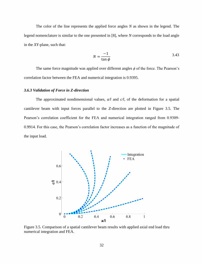
3.6.3 Validation of Force in Z-direction

The approximated nondimensional values, a/l and c/l, of the deformation for a spatial

cantilever beam with input forces parallel to the Z-direction are plotted in Figure 3.5. The

Pearson’s correlation coefficient for the FEA and numerical integration ranged from 0.9309-

0.9914. For this case, the Pearson’s correlation factor increases as a function of the magnitude of

the input load.

Figure 3.5. Comparison of a spatial cantilever beam results with applied axial end load thru

numerical integration and FEA.

33

3.6.4 Validation of Force in the YZ-plane

The results a/l versus b/l and a/l versus c/l for an applied load in the YZ-plane at different

angles are plotted in Figure 3.6a and Figure 3.6b, respectively. For both plots, the magnitude of

the force remained constant as the input angles of the load varied in the YZ-plane. In these plots,

the dots represent the results via FEA while the lines represent the results obtained by numerical

integration. The color of the line represents the applied force angle. The Pearson’s correlation

coefficient for the FEA and numerical integration for the displacement in the y-direction ranged

from 0.9454-0.9895 and for the z-direction displacement is 0.8858 - 0.9191.

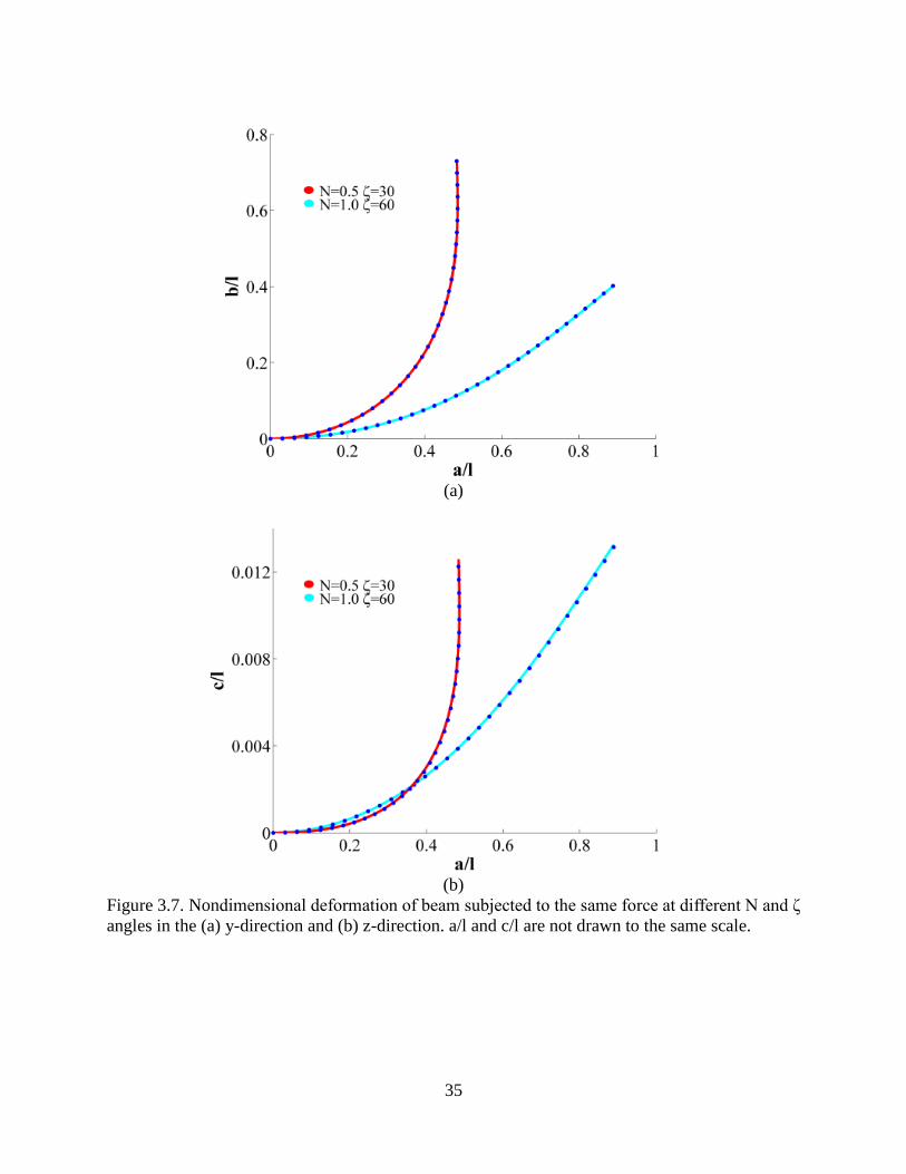
3.6.5 Validation of General XYZ Forces

To validate the equations, the same force magnitude was applied to a beam at two

different angles as shown in Figure 3.7a and Figure 3.7b. At N=116.6 and ζ=30 degrees, the

Pearson’s correlation factor is 0.7506 in the x-direction, 0.9556 in the y-direction and 0.8870 in

the z-direction. At N=153 and ζ=60 degrees, the Pearson’s correlation factor is 0.9957 in the x-

direction, 0.9168 in the y-direction and 0.9149 in the z-direction.

34

(a)

(b)

Figure 3.6. Deformation results of a beam in the (a) y-direction and (b) z-direction with inclined

load via integration (line) and FEA (dots). a/l and c/l are not drawn to the same scale.

35

(a)

(b)

Figure 3.7. Nondimensional deformation of beam subjected to the same force at different N and ζ

angles in the (a) y-direction and (b) z-direction. a/l and c/l are not drawn to the same scale.

36

Chapter 4

Axisymmetric Pseudo-Rigid-Body Model2

The objective of this chapter is to describe kinematic models, pseudo-rigid-body models

(PRBMs), for approximating the spatial deflection of an elastic beam with axisymmetric cross-

section. The equations that predict the rotation, curvature and location of the beam’s neutral axis

as function of the arclength were derived in Chapter 3. PRBMs modeling the kinematics and

stiffness of an axisymmetric cantilever beam with force end-loads and with moment end-loads

are presented. Also, approximations for the characteristic radius factor and the parametric

coefficient for moment loading as a function of the tip angle are presented.

4.1 Axisymmetric Pseudo-Rigid-Body Model

In an axisymmetric cantilever beam, Izz is equal to Iyy. The change in the curvature of the

beam can be expressed as follows:

𝑑𝜏𝑥

𝑑𝑠=

1


𝑑𝜅𝑦

𝑑𝑠=

1

EI𝑦𝑦

[(𝐸𝐼𝑧𝑧 − 𝐺𝐼𝑥𝑥)τ𝑥,𝜅𝑧 , + 𝐹𝑧′] 4.2

𝑑𝜅𝑧

𝑑𝑠=

1

EI𝑧𝑧[(𝐺𝐼𝑥𝑥 − 𝐸𝐼𝑦𝑦)τ𝑥,𝜅𝑦, + 𝐹𝑦′]

4.3

_________________________ 2Portions of this chapter were previously published in [44]. Permission is included in Appendix A.

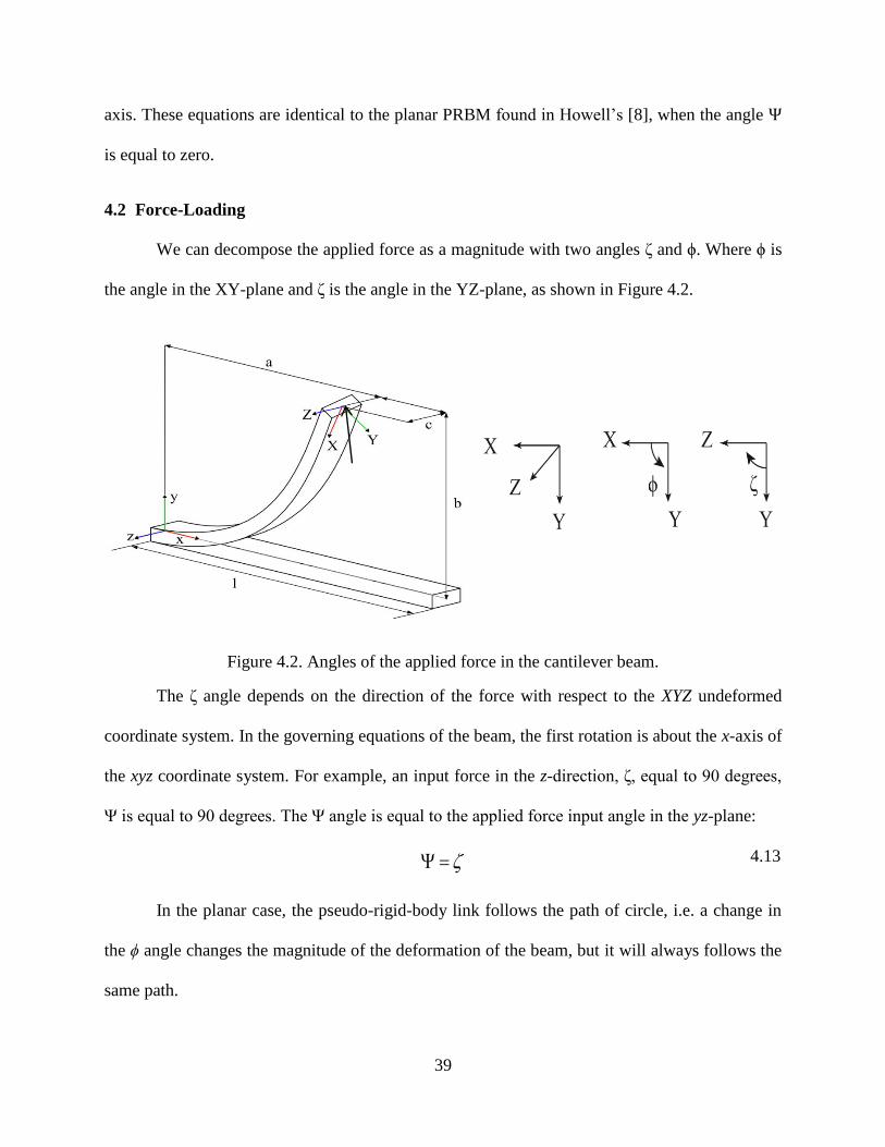
37

Thus, the change in torsion, dtx/ds, is zero because the moment of inertia Izz is equal to Iyy,

Therefore, the torsion is constant throughout the beam. When there is no applied torque on the

free-end (τx(s=0) = 0), the torsion (twisting of the beam about the neutral axis) is equal to zero

(τx(s) = 0). The governing curvature equations for an axisymmetric beam with no torsion become:

𝑑𝜏𝑥

𝑑𝑠= 0

4.4

𝑑𝜅𝑦

𝑑𝑠=

𝐹𝑧′

EI𝑒𝑞 4.5

𝑑𝜅𝑧

𝑑𝑠=

𝐹𝑦′

EI𝑒𝑞 4.6

where Ieq = Iyy = Izz, E is the Young’s Modulus, and 𝐹𝑦′ and 𝐹𝑧′ is the force expressed in the x’y’z’

frame, as stated in Chapter 3, such that:

𝐹𝑦′ = [cos 𝜃 cos𝜓 sin𝜙 + sin𝜓 cos𝜙]𝐹𝑦 − sin 𝜃 sin𝜙 𝐹𝑥 +

[cos 𝜃 sin𝜓 sin𝜙 − cos𝜓 cos𝜙]𝐹𝑧

4.7

𝐹𝑧′ = [cos 𝜃 cos𝜓 cos𝜙 − sin𝜓 sin𝜙]𝐹𝑦 − sin 𝜃 cos𝜙 𝐹𝑥 +

[cos 𝜃 sin𝜓 cos𝜙 − cos𝜓 sin 𝜙]𝐹𝑧

4.8

where 𝜙, 𝜃, and 𝜓 are the Euler angles and Fx, Fy and, Fz are the forces applied to the beam with

respect to the xyz coordinate system, as discussed in Chapter 3. Because the 𝜙 rotation is defined

by the amount that the {p}-frame must be rotated about the neutral axis, so that Izz is the smallest

principal moment of area and Iyy is the larger principal moment of area. Because in an

axisymmetric beam the moments of area are equal, 𝜙 becomes arbitrary and may be chosen as

𝜙(𝑠) = 0. Thereby, Equation 3.12 requires that:

𝑑𝜙

𝑑𝑠= −

𝑑𝜓

𝑑𝑠cos 𝜃 4.9

38

Thus 𝜓(𝑠) is constant. This means that the beam stays in the same plane because the

rotations of each beam segment are about parallel axes.

One can assume a PRBM for an axisymmetric cantilever beam similar to the one

presented in [8], attaching a spherical joint instead of a revolute joint, to allow rotation about the

x, y and z-axes. The PRBM consists of two rigid links connected by a spherical joint, as shown in

Figure 4.1. The spherical joint is located at γl distance from the free-end of the cantilever beam,

allowing the rotation of the pseudo-rigid-body link, and thus, the displacement of its tip.

Figure 4.1. Axisymmetric PRBM of a cantilever beam.

The kinematic equations of the cantilever beam can be found by means of spherical

trigonometry. The tip coordinates (as, bs, cs) of the spatial PRBM of a cantilever beam with end

loads are given by:

𝑎𝑠 = 𝑙 − 𝛾𝑙(1 − cos Θ) 4.10

𝑏𝑠 = 𝛾𝑙 sinΘ cosΨ 4.11

𝑐𝑠 = 𝛾𝑙 sinΘ sinΨ 4.12

where l is the length of the beam, γ is the characteristic radius factor, Θ is the rotation angle of

the beam with respect to the z-axis, and Ψ is the rotation angle of the beam with respect to the x-

39

axis. These equations are identical to the planar PRBM found in Howell’s [8], when the angle Ψ

is equal to zero.

4.2 Force-Loading

We can decompose the applied force as a magnitude with two angles ζ and ϕ. Where ϕ is

the angle in the XY-plane and ζ is the angle in the YZ-plane, as shown in Figure 4.2.

Figure 4.2. Angles of the applied force in the cantilever beam.

The ζ angle depends on the direction of the force with respect to the XYZ undeformed

coordinate system. In the governing equations of the beam, the first rotation is about the x-axis of

the xyz coordinate system. For example, an input force in the z-direction, ζ, equal to 90 degrees,

Ψ is equal to 90 degrees. The Ψ angle is equal to the applied force input angle in the yz-plane:

4.13

In the planar case, the pseudo-rigid-body link follows the path of circle, i.e. a change in

the ϕ angle changes the magnitude of the deformation of the beam, but it will always follows the

same path.

40

The governing equations of the beam employ a follower load at the end of the beam, to

acquire the deflection of the beam’s tip and the non-follower forces of the beam. The governing

equations are convenient to analyze beams subjected to follower loads; to obtain the non-

follower loads requires to know the rotations of the Euler angles which makes the comparison

with non-follower results difficult. In order to compare with non-follower based PRBM, a Finite

Element Analysis (FEA) program was used to calculate the deflection of the beam instead of the

governing equations. In the FEA program, the main input are the non-follower forces, whereas in

the governing equation model of the beam, only follower forces yields the exact results for an

applied force load, as shown in Chapter 3. Therefore, an FEA program (Ansys) was used to

obtain non-follower load results.

Inclined non-follower forces in the xy and yz-plane were applied to the cantilever beam in

a finite element analysis program. The non-follower forces applied to the cantilever ranged from

3.0 x103

N to 3.0 x105

N in increments of 3.0 x103

N, keeping a constant angle of inclination of

ϕ=116.6 degrees. The force angle in the xy-plane was kept at ϕ=116.6 degrees, but the force

angle in the yz-plane was changed.

With the exact values of the deflection of the beam obtained thru FEA analysis, the exact

values of the pseudo-rigid-body parameters are found through an optimization routine solving

Equations 4.10 - 4.12. For example, a force magnitude of 7.5 x 104 N was applied to the beam at

an angle of ϕ=116.6 degrees in the xy-plane, and ζ=30 degrees in the yz-plane. The

nondimensional deflection coordinates of the beam’s tip are a/l= 0.47190, b/l= 0.67509 and, c/l=

0.38976. The PRBM parameters found via the optimization routine are γ= 0.8394, ϴ= 1.1909

radians (68.2326 degrees) and, Ψ= 0.523599 radians (30.0 degrees). One can notice that the

angle Ψ is equal to the input angle ζ in the yz-plane, as stated in Equation 4.13.

41

The one revolute joint (1R) PRBM parameters from Howell’s [8], can be used to find the

axisymmetric spatial PRBM. The 1R PRBM equations from [8] are:

𝑎𝑝 = 𝑙 − 𝛾𝑙(1 − cos Θ) 4.14

𝑏𝑝 = 𝛾𝑙 sinΘ 4.15

This set of equations can be used to find the horizontal and vertical coordinates of the

beam (ap, bp) given the magnitude and the angle of inclination of the force in the xy-plane and

the geometric parameters. These coordinates were rotated from their planar position by a rotation

of the x-axis:

[

𝑎𝑠

𝑏𝑠

𝑐𝑠

] = [1 0 00 cosΨ − sinΨ0 sinΨ cosΨ

] [

𝑎𝑝

𝑏𝑝

0

] 4.16

Figure 4.3 shows the path of the spatial PRBM and the FEA when an inclined non-

follower load in the xyz coordinate system is applied to the beam. The angle in the xy-plane was

kept at n=0.5 (ϕ=116.6 degrees). For the PRBM calculation, the characteristic radius used was

the approximation for 0.5 < 𝑛 ≤ 10.0 is [8]:

𝛾 = 0.841655 − .0067807𝑛 + .000438004𝑛 4.17

Three cases were studied: when ζ=30, 45, and 60 degrees. The dots represent the PRBM

results and the line represents the FEA results. The parameters are shown in Table 4.1.

Therefore, the planar PRBM parameters work for an axisymmetric beam when the planar

results are multiplied by a rotation in the x-direction.

42

(a)

(b)

Figure 4.3. Path results for FEA and spatial PRBM in the (a) y-direction and (b) z-direction.

43

Table 4.1. Parameters used in the validation of the axisymmetric spatial PRBM.

Parameters Value

w (m) 0.1

h (m) 0.1

l (m) 10

E (GPa) 207 x109

ν 0.33

ΔF 3.0 x103

ϕ (degrees) 116.6°

4.3 Moment Input

Non-follower in-plane moments, Mz, and out-of-plane moments, My, were applied in the

governing equations of the axisymmetric beam. With multiple moments, the pseudo-rigid-body

angle with respect to the z-axis is ϴ, and the rotation of the xy-plane about the x-axis is the

pseudo-rigid-body angle Ψ, as shown in Figure 4.1. The PRBM parameters for a planar beam

with an in-plane applied moment are found as shown in [8].

4.3.1 Out-of-Plane Moment Only (My only)

The pseudo-rigid-body model for a planar axisymmetric beam with an out-of-plane

moment, My, is shown in Figure 4.4. The PRBM is similar to the one found in [8], but applying

an out-of-plane moment My, which consists of two links connected through a revolute joint.

The kinematic equations of the cantilever beam can be found by setting the value Ψ equal

to 90 degrees in Equations 4.10-4.12. The end-tip coordinates of the spatial PRBM (as, cs) of a

cantilever beam with a My load are given by:

𝑎𝑠 = 𝑙 − 𝛾𝑙(1 − cosΘ) 4.18

44

𝑏𝑠 = 0

4.19

𝑐𝑠 = 𝛾𝑙 sinΘ 4.20

where l is the length of the beam, γ is the characteristic radius factor and, ϴ is the rotation angle

of the beam with respect to the z-axis.

Figure 4.4. PRBM for an axisymmetric beam with an applied out-of-plane moment.

A series of out-of-plane moments were applied to a cantilever beam in order to calculate

the exact deflection of the beam. Figure 4.5 presents the nondimensional path of the one revolute

joint (1R) PRBM and the results of the kinematic equations, using Howell’s pseudo-rigid-body

parameters [8], where γ = 0.7346 and cθ = 1.5164. With these parameters, the relative deflection

error (Equation 2.16), between the results of the kinematic equations and the 1R PRBM at the tip

angle of 124 degrees is 1.4070%, as shown in Figure 4.6.

45

Figure 4.5. Nondimensional path results from the 1R PRBM and numerical equations for a beam

with an applied moment in the y-direction, My.

Figure 4.6. Relative deflection error of a cantilever beam versus the tip angle.

46

To minimize the relative deflection error, the exact values of the characteristic radius

parameter and the parametric angle coefficient can be found through optimization of the

coordinates. The nondimensional theoretical coordinates from the Bernoulli-Euler large-

deflection equations depend only on the tip slope of the beam’s end, as stated in Equations 2.34

and 2.37. Substituting tip angles from 0 to 124.4 degrees, the theoretical coordinates of the

deflection of the beam can be found. Knowing the deflection of the beam’s end, the exact PRB

parameters can be calculated by replacing the theoretical coordinates into Equations 4.18 and

4.20. A polynomial fitting routine was implemented to find the governing equation that describes

the characteristic radius factor and the parametric coefficient as a function of the tip angle as

shown in Figure 4.7 and Figure 4.8, respectively.

Figure 4.7. Exact value of the characteristic radius factor for different tip angles.

y = -0.0047x2 + 0.0006x + 0.7499

R² = 0.9999

0.725

0.73

0.735

0.74

0.745

0.75

0.755

0 0.5 1 1.5 2 2.5

γ

θo (rad)

47

Figure 4.8. Exact value of the parametric angle coefficient for various tip angles.

From the polynomial fitting curve, the equation that relates the approximated value of the

characteristic radius factor as a function of the tip angle for planar beams is given by:

𝛾𝑎 = −0.0047 𝜃02 + 0.0006𝜃0 + 0.7499 4.21

The relation between the tip angle and the approximated parametric angle coefficient is:

𝑐𝜃𝑎 = 0.0063 𝜃02 + 0.0010𝜃0 + 1.5002 4.22

where the tip angle is measured in radians. Substituting the approximated values of the

characteristic radius factor and the approximated values of the parametric angle coefficient in

Equations 4.18 and 4.20, the path results of the 1R PRBM are plotted in Figure 4.9. Moment

loads of 0 to 5x105

Nm, increased by 1x104 Nm were applied to the cantilever beam. These sets

of loads have tip angles ranging from 0 to 172.71 degrees. The squares in Figure 4.9 represent

the results from the kinematic equations, and the dots stand for the results given by the

y = 0.0063x2 - 0.0010x + 1.5002

R² = 0.9999

1.495

1.5

1.505

1.51

1.515

1.52

1.525

1.53

0 0.5 1 1.5 2 2.5

c θ

θo (rad)

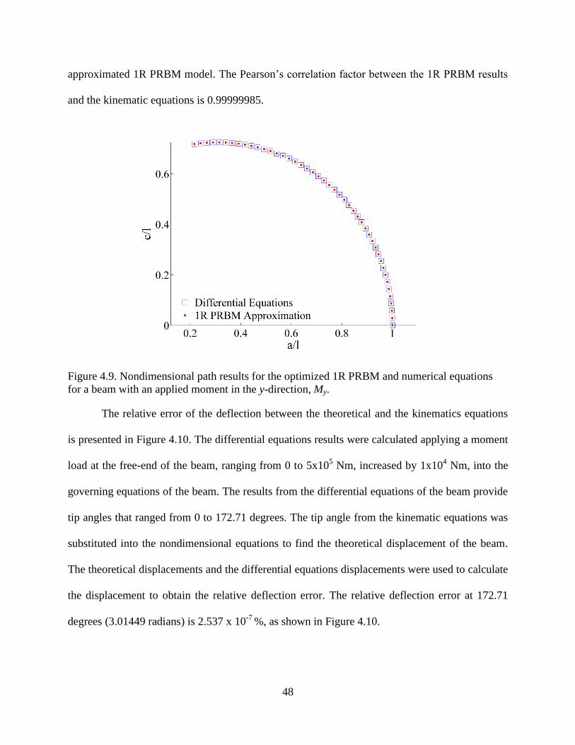
48

approximated 1R PRBM model. The Pearson’s correlation factor between the 1R PRBM results

and the kinematic equations is 0.99999985.

Figure 4.9. Nondimensional path results for the optimized 1R PRBM and numerical equations

for a beam with an applied moment in the y-direction, My.

The relative error of the deflection between the theoretical and the kinematics equations

is presented in Figure 4.10. The differential equations results were calculated applying a moment

load at the free-end of the beam, ranging from 0 to 5x105 Nm, increased by 1x10

4 Nm, into the

governing equations of the beam. The results from the differential equations of the beam provide

tip angles that ranged from 0 to 172.71 degrees. The tip angle from the kinematic equations was

substituted into the nondimensional equations to find the theoretical displacement of the beam.

The theoretical displacements and the differential equations displacements were used to calculate

the displacement to obtain the relative deflection error. The relative deflection error at 172.71

degrees (3.01449 radians) is 2.537 x 10-7

%, as shown in Figure 4.10.

49

Figure 4.10. Relative deflection error between the theoretical and the governing equations of a

cantilever beam.

In previous compliant mechanisms work, the maximum tip angle for a 1R PRBM to

achieve a relative deflection error of 0.5% was 124.4 degrees [8]. The relative deflection error

for a beam with a single moment applied at the end, using the approximated values of the

characteristic radius factor and the approximated parametric coefficient, for a tip angle of 124.4

degrees, is 0.011%, as shown in Figure 4.11. This approximation provides an improvement to

previous published parameters, increasing the tip angle to 169.76 degrees (2.96294 radians),

where the relative error is 0.5%.

4.3.1.1 Energy Methods Using PRBMs

In force loaded pseudo-rigid-body models (PRBMs) the energy stored in the torsional

spring is equal to the energy stored in the deformed beam. This is not true in moment loaded

beams as shown in this section.

50

Figure 4.11. Relative deflection error of a cantilever beam versus the input angle of the applied

moment load.

The PRBM with a single applied out-of-plane end-moment is shown in Figure 4.4.

Assuming no energy is loss in the system, the potential energy of a spring is given by:

𝑉 =1

2𝐾𝑠Θ

2 4.23

where the spring constant, Ks, and the beam end angle. The relationship between the end-slope

angle and the spring constant in terms of the PRBM parameters are given by:

𝐾𝑠 = 𝛾𝐾𝜃𝐸𝐼/𝑙 4.24

where 𝛾 is the characteristic radius factor, 𝐾𝜃 is the stiffness coefficient, E is the Young’s

Modulus, I is the moment of inertia and l is the length of the beam. For a moment end-load, the

relationship can be simplified to:

𝐾𝑠 = 𝑐𝜃𝐸𝐼/𝑙 4.25

𝜃0 = 𝑐𝜃Θ 4.26

51

where 𝑐𝜃 is the parametric angle coefficient. In the case of a single spring, the potential energy is

equal to the strain energy. After substitution of Equations 4.25 and 4.26 in the spring potential

energy formula (Equation 4.23), the energy due to a spring is given by:

𝑉 =𝐸𝐼θ0

2

2𝑙𝑐𝜃 4.27

Using elastic theory, the strain energy of stored in a beam given an input moment is given

by:

𝑈 = ∫𝑀0

2𝑑𝑠

2𝐸𝐼 4.28

where the moment at the end of the beam is given by:

𝑀0 =𝐸𝐼θ0

𝑙 4.29

Substituting Equation 4.29 of the moment at the end of the beam in the strain energy

Equation 4.28 and integrating, the potential energy of a flexible beam is found to be:

𝑈 =𝐸𝐼θ0

2

2𝑙 4.30

Combining Equations 4.27 and 4.30, the potential energy of the spring, V, and the strain

energy stored in the beam, U, for a beam with end-moment loading, are related as:

𝑈 = 𝑐𝜃𝑉 4.31

The stiffness of a beam depends in the material properties and the geometry. The stiffness

of a beam is the product of the moment of inertia and the Young’s Modulus. The stiffness of a

beam in relation with the one of the PRBM can be derived in a similar manner that the potential

energy. The stiffness of a flexible beam, Kf, and stiffness of the PRBM are related by:

𝐾𝑓 = 𝑐𝜃𝐾𝑠 4.32

52

Following the nomenclature of compliant mechanisms, the stiffness coefficient, Kϴ is:

𝐾Θ = 𝑐𝜃𝐾𝑠 4.33

The difference in the PRBM spring energy and the beams strain energy means that

caution must be used in evaluating PRBMs using moment loaded segments.

4.3.2 Multiple Loading: My and Mz

Non-follower in-plane and out-of-plane moments, Mz and My, respectively, were applied

to the axisymmetric beam. The torsion (twisting of the beam about the neutral axis) is constant

throughout the beam. The curvature equations in the follower frame become:

0

ds

d x

4.34

0

ds

d y 4.35

0ds

d z 4.36

The change of the curvature of an axisymmetric cantilever beam with applied multiple

moments is zero. Thus, the curvature remains constant through the beam.

The pseudo-rigid-body angle with respect to the z-axis is ϴ, and the pseudo-rigid-body

angle with respect to the x-axis is Ψ, are shown in Figure 4.1. For axisymmetric beams, the Ψ

angle depends on the direction of the applied moment with respect to the xyz undeformed

coordinate system.

Figure 4.12 and Figure 4.13 shows the path of the spatial PRBM and the differential

equations when an inclined non-follower load in the xyz coordinate system is applied to the

beam. Three different paths were studied, when Mz is 4.0 x104 Nm (cyan), 2.0 x10

5 Nm (green)

and 3.6 x105 Nm (magenta).

53

Figure 4.12 presents the horizontal deflection versus the in-plane bending. The dots

represent the approximated 1R PRBM results, and the line represents the differential equations

results. The Pearson’s correlation factor between the differential equations and the 1R PRBM is

0.999823.

Figure 4.12. Horizontal versus in-plane deflection for various cases. Line represents the

differential equations results and the dots the deflection of the 1R PRBM.

Figure 4.13 presents the horizontal deflection (as/l) versus the out-of-plane bending (cs/l).

The dots represent the 1R PRBM results and the line represents the differential equations results.

The Pearson’s correlation factor between the optimized parameters of the PRBM and the results

from the spatial differential equations is 0.9997.

54

Figure 4.13. Horizontal versus out-of-plane deflection for varius cases. Line represents the

differential equations results and the dots the deflection of the 1R PRBM.

4.3.2.1 Relative Deflection Error for a Spatial Beam

The relative deflection error for a spatial beam can be found in a similar manner to the

relative deflection error for a planar beam. The true value of the deflection (at, bt, ct) can be

found thru numerical integration of the deflection of the beam. The theoretical value of the

deflection, 𝛿𝑡, where at is the deflection with respect to the x-axis, bt is the deflection with

respect to the y-axis, ct is the deflection with respect to the z-axis and L is the length of the beam,

can be found as:

𝛿𝑡 = √(𝐿 − 𝑎𝑡)2 + 𝑏𝑡

2 + 𝑐𝑡2 4.37

The pseudo-rigid-body model deflection approximated value, 𝛿𝑎, can be found by:

𝛿𝑎 = √[𝛾𝐿(1 − cosΘ]2 + [𝛾𝐿 sinΘ cosΨ]2 + [𝛾𝐿 sinΘ sinΨ]2 4.38

where γ is the characteristic radius factor and ϴ and Ψ are the pseudo-rigid-body angles with

respect to the z-axis and x-axis, respectively. The error in the deflection is:

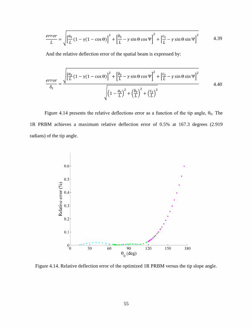
55


𝐿= √[

𝑎𝑡

𝐿(1 − γ(1 − cosΘ)]

2

+ [𝑏𝑡

𝐿− 𝛾 sinΘ cosΨ]

2

+ [𝑐𝑡

𝐿− 𝛾 sinΘ sinΨ]

2

4.39

And the relative deflection error of the spatial beam is expressed by:


𝛿𝑡=

√[𝑎𝑡𝐿

(1 − γ(1 − cosΘ)]2+ [

𝑏𝑡𝐿

− 𝛾 sinΘ cosΨ]2

+ [𝑐𝑡𝐿

− 𝛾 sinΘ sinΨ]2

√(1 −𝑎𝑡𝐿

)2+ (

𝑏𝑡𝐿

)2

+ (𝑐𝑡𝐿)2

4.40

Figure 4.14 presents the relative deflections error as a function of the tip angle, θ0. The

1R PRBM achieves a maximum relative deflection error of 0.5% at 167.3 degrees (2.919

radians) of the tip angle.

Figure 4.14. Relative deflection error of the optimized 1R PRBM versus the tip slope angle.

56

4.3.2.2 Stiffness for Multiple Moment Loading

Non-follower in-plane moments, Mz, and out-of-plane moments, My, were applied to the

beam. The magnitude of the applied moment is equal to:

|𝑀0| = √𝑀𝑧2 + 𝑀𝑦

2 4.41

The in-plane to the out-of-plane moments can be related by means of the nondimensional

factor ε, using the following relation:

휀 =𝑀𝑧

𝑀𝑦 4.42

Substituting Equation 4.42 into Equation 4.43, the magnitude of the applied moment the

end of the beam can be written as:

|𝑀0| = 𝑀𝑧√1 + 휀2 4.43

The beams resistance to deflection is modeled by the torsional spring, Ks. Because the

geometric and material properties are considered in the in-plane torsional constant, Ks, in

Equation 4.25, the value of the magnitude of the combined torsion spring, Ksc, can be defined as:

𝐾𝑠𝑐 = 𝐾𝑠√1 + 휀2 4.44

The magnitude of the torque in the spring can be found by rotating Ψ around the x-axis,

simplifying:

𝑇𝑐 = (cosΨ − sinΨ) 𝐾𝑠𝑐Θ 4.45

The magnitude of the spring torque, Equation 4.45, was compared to the magnitude of

the input moment. An input in-plane moment, Mz, was applied to the end of the beam, and an

out-of-plane moment My was increased by the nondimensional factor, ε. Three cases were

studied: (1) when Mz is 0.8x105 Nm, (2) when Mz is 2.0 x10

5 Nm and, (3) when Mz is 4.0 x10

5

Nm. The PRBM parameters used are specified in Table 4.2.

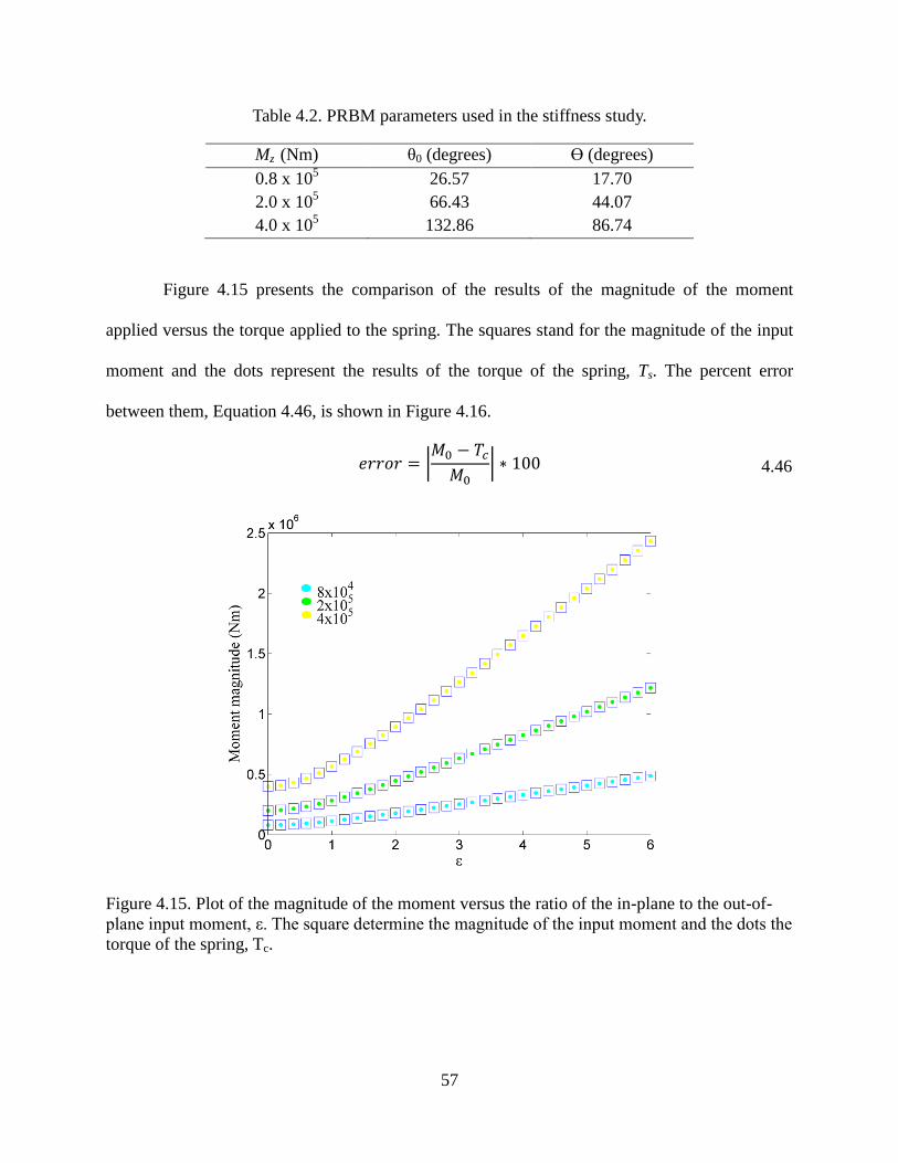
57

Table 4.2. PRBM parameters used in the stiffness study.

Mz (Nm) θ0 (degrees) ϴ (degrees)

0.8 x 105 26.57 17.70

2.0 x 105 66.43 44.07

4.0 x 105 132.86 86.74

Figure 4.15 presents the comparison of the results of the magnitude of the moment

applied versus the torque applied to the spring. The squares stand for the magnitude of the input

moment and the dots represent the results of the torque of the spring, Ts. The percent error

between them, Equation 4.46, is shown in Figure 4.16.

𝑒𝑟𝑟𝑜𝑟 = |𝑀0 − 𝑇𝑐

𝑀0| ∗ 100 4.46

Figure 4.15. Plot of the magnitude of the moment versus the ratio of the in-plane to the out-of-

plane input moment, ε. The square determine the magnitude of the input moment and the dots the

torque of the spring, Tc.

58

Figure 4.16. Percentage error between the applied moment at the end of the beam and the spring

torque.

4.4 Conclusion

For a cantilever beam with no torques, the planar PRBM results from Howell [8], Feng

[35] and Su [37] can be used to define an axisymmetric PRBM. The force vector and the

moment applied at the beam tip and the axis of the beam itself are used to define a plane whose

angular deviation from the xy-plane is described by the angle Ψ. An axisymmetric PRBM is then

given when the planar results are multiplied by a rotation in the x-direction:

𝑅𝑥 = [1 0 00 cosΨ − sinΨ0 sinΨ cosΨ

] 4.47

The characteristic radius factor and the PRB angle coefficient for a beam with a single

moment applied at the end were optimized to minimize the error incurred using the deflection

formulas of the PRBM. This approximation provides an improvement to previous published

parameters, providing a relative error of 0.5% at a tip slope angle to 169.76 degrees (2.96294

radians).

59

In force loaded Pseudo-Rigid-Body Models (PRBMs) the energy stored in the torsional

spring is equal to the energy stored in the deformed beam. In moment loaded beams, the PRBM

spring energy and the beams strain energy are related by the parametric angle coefficient. This is

because the parametric angle coefficient is the ratio between the tip angle and the PRB angle Θ.

This means that caution must be used in evaluating PRBMs using moment loaded segments.

60

Chapter 5

Rectangular Pseudo-Rigid-Body Model with Bending Moment Loads

The objective of this chapter is to develop a pseudo-rigid-body model (PRBM) for a

rectangular cantilever beam that undergoes planar and out-of-plane bending moments. The

governing equations of the beam that were derived in Chapter 3 are used to calculate the

deflection, rotation and curvature of the beam’s neutral axis as a function of the arclength. A

PRBM modeling the kinematics and stiffness of a spatial cantilever beam with bending moment

loads is presented. With the governing equations of the beam, the PRBM and equations from

virtual work, the PRBM parameters were developed.

5.1 Governing Equations of a Beam

The equations that describe deflection, rotation and curvature of a beam that experiences

forces and moments were derived in Chapter 3. Because in the analysis presented in this chapter

force loads are not considered, 𝐹𝑦′ and 𝐹𝑧′ are set to zero in the {h}-frame. The differential

equations were derived with s=0 at the free-end of the cantilever beam, assuming no

displacements or rotations in the {a}-frame. Equations 5.1-5.9 can be used to find the Euler

angles (𝜙, 𝜃, and 𝜓) the curvatures (𝜏𝑥, 𝜅𝑦 and 𝜅𝑧), and the coordinates (X, Y and Z) with respect

to the arclength (s) for a beam that undergoes bending moments at the free-end.

𝑑𝜙

𝑑𝑠= τ𝑥, + 𝜅𝑦, cos𝜙

cos 𝜃

sin 𝜃− 𝜅𝑧 , sin𝜙

cos 𝜃

sin 𝜃 5.1

61

𝑑θ

𝑑𝑠= 𝜅𝑦, sin𝜙 + 𝜅𝑧 , cos 𝜙 5.2

𝑑𝜓


cos𝜙


sin𝜙

sin 𝜃 5.3

𝑑𝜏𝑥

𝑑𝑠=

1


𝑑𝜅𝑦

𝑑𝑠=

1

EI𝑦𝑦

(𝐸𝐼𝑧𝑧 − 𝐺𝐼𝑥𝑥)τ𝑥,𝜅𝑧 , 5.5

𝑑𝜅𝑧

𝑑𝑠=

1

EI𝑧𝑧(𝐺𝐼𝑥𝑥 − 𝐸𝐼𝑦𝑦)τ𝑥,𝜅𝑦, 5.6

𝑑X

𝑑𝑠= cos 𝜃 5.7

𝑑Y

𝑑𝑠= sin 𝜃 cos𝜓 5.8

𝑑Z

𝑑𝑠= sin 𝜃 sin𝜓 5.9

The ODE45 command in Matlab was used to numerically integrate the differential

equations, where the interval of integration from the negative of the length of the beam to zero.

The planar moment (Mz) and the out-of-plane moments (My) are applied in the free-end of the

beam as follower loads, thus both moments are at 90 degrees of each other in the {h}-frame. The

non-follower moments at the fixed frame are found by rotating the follower moments by the

angles 𝜙, 𝜃, and 𝜓:

�� 𝑎 = 𝑅𝑝𝑎 ( 𝑥𝑎 , 𝜙 ) 𝑅𝑞

𝑝 ( 𝑧𝑝 , θ ) 𝑅ℎ𝑞 ( 𝑥𝑞 , 𝜓 ) �� ℎ 5.10

where the {a}-frame is the fixed frame and the {h}-frame is the follower frame at the beams tip.

Similarly, the coordinates of the beam tip (a,b,c) with respect to the fixed end of the beam can be

found as:

62

[ 𝑥𝑎 , 𝑦𝑎 , 𝑧𝑎 ]′ = 𝑅𝑝𝑎 ( 𝑥𝑎 , 𝜙 ) 𝑅𝑞

𝑝 ( 𝑧𝑝 , θ ) 𝑅ℎ𝑞 ( 𝑥𝑞 , 𝜓 )[ 𝑋ℎ , 𝑌ℎ , 𝑍ℎ ]′ 5.11

The governing equations of the beam are valid for any magnitude of applied loads; this

means that the tip can undergo more than 360 degrees rotation. Because we are only interested in

solutions to the Equations 1.1-1.9 that can be reasonably approximated with a two-link pseudo-

rigid-body model, the rotation of the beam tip with respect to the fixed end was restricted. The

magnitude of the applied planar moment (Mz) in the follower frame was calculated as follows:

𝑀𝑧ℎ =

𝜃𝑖𝐸𝐼𝑧𝑧𝑙⁄

5.12

where 𝜃𝑖 is the initial tip angle, l is the length of the beam, E is the Elastic modulus and Izz is the

moment of inertia with respect to the z-axis. The initial tip angle was restricted to 120 degrees,

which ensures that the PRBM parameters can be related to the planar PRBM parameters

developed by Howell [8].

Perturbation theory can be used to apply the out-of-plane moment (My) such that it

ensures the applied load does not produce excessive out-of-plane deflection. The perturbation

method provides a simple method to find the approximate solution to a difficult problem in terms

of a power series. In the perturbation method, the effect of a dimensionless small parameter, 휀, is

introduced in the differential equations to find a solution to the problem. Three steps are

fundamental in a perturbation analysis [42]:

1. Convert the original problem into a perturbation problem by introducing a small parameter,

휀.

2. Assume an expression for the answer in the form of a perturbation series and compute the

coefficients of that series. In this step, the unperturbed problem is solved by obtaining the

solution when 휀 =0 in the problem.

63

3. Recover the answer to the original problem by assuming the perturbation series for the

appropriate value of 휀.

Using the perturbation method, a follower out-of-plane end-moment load will be applied

to a cantilever beam with in-plane moments.

𝑀𝑦ℎ = 휀 𝑀𝑧

ℎ 5.13

The small parameter, 휀, will give a measure of the magnitude of the applied out-of-plane

moment with respect to the in-plane moment, as shown in Figure 5.1.

Figure 5.1. Diagram of a cantilever beam with applied moment-loading.

5.2 Rectangular Pseudo-Rigid-Body Model

One can assume a PRBM for a rectangular cantilever beam similar to the one presented

in Chapter 4 for the axisymmetric beam. The PRBM consists of two rigid links connected by a

spherical joint and a spherical cap, as shown in Figure 5.2. The spherical joint is located at γl

distance from the free-end of the cantilever beam and allows the rotation of the pseudo-rigid-

body link, and thus the displacement of its tip.

64

Figure 5.2. PRBM of a cantilever beam with moment loads.

The position of the tip end (as, bs, cs) of the spatial PRBM of a cantilever beam with end

loads is given by:

𝑎𝑠 = 𝑙 − 𝛾𝑙(1 − cos Θ) 5.14


𝑐𝑠 = 𝛾𝑙 sinΘ sinΨ 5.16

where l is the length of the beam, γ is the characteristic radius factor, ϴ is the characteristic bend

angle of the beam with respect to the z-axis and, Ψ is the characteristic twist angle of the beam

with respect to the x-axis.

In Chapter 4, we presented a PRBM for a beam that undergoes planar motion that allows

the rotation of the pseudo-rigid-body link, and thus, the displacement of its tip. Two frames were

sufficient to specify the deflection of the free-end of the beam. However, in order to describe the

orientation of the beam end, a spherical cap in the tip of the beam was added to the PRBM.

To specify the orientation of the beam, we can assume another set of XZX rotations, by

the angles Σ, Ω, and Φ. As shown in Figure 5.3, the {a}-frame, which is located at the fixed end

65

of the beam, is twisted by the characteristic twist angle Ψ. The characteristic bend angle Θ is the

intersection of the plane XY-plane which contains the PRB link. The Σ angle can be viewed as

the torsion in the longer PRB link. The rotation angles Ω and Φ are the rotation in the z-direction

and the x-direction of the beams tip, respectively.

Figure 5.3. The frames and the PRBM angles from the fixed to the free-end of the beam.

The twisting components of is composed of two angles Γ and Υ:

𝑅𝑎

𝑐 ( 𝑥𝑎 , Ψ) = 𝑅𝑏𝑐 ( 𝑥𝑏 , Γ) ∗ 𝑅𝑎

𝑏 ( 𝑥𝑎 , Υ) 5.17

Because Γ and Υ have the same axis,

Ψ𝑎

𝑐 = Γ𝑏𝑐 + Υ𝑎

𝑏 5.18

where ϒisthe torsion of the shorter PRB segment and is the orientation of the bend direction.

Because there are five kinematic variables ( , , , and , and only three load

variables (Mx, My, and Mz), the kinematic variables are not all independent and cannot all be used

as generalized coordinates for virtual work equations. By comparison with the planar model and

inspection of the data, we find that is dependent on , such that:

Ω = 𝑐ΩΘ 5.19

where 𝑐Ω is the PRB-link parametric angle coefficient. The angle Φ is also dependent, bot has a

more complicated relationship to the independent variables Γ, Σ, Θ, and Ψ.

5.2.1 Virtual Work

The principle of virtual work states that “the net virtual work of all active forces is zero if

and only if an ideal mechanical system is in equilibrium”[8]. The method of virtual works is a

a-Frame (Fixed)

Ψ Θ Σ Ω Φ h-Frame

(Tip)

a c d e f h

66

useful tool to develop force and deflection relationships. Using the method of virtual work, the

equilibrium positions of a system acted on a pure moment is given by:

�� ∙ 𝑑𝜃 − ∑𝑑𝑉𝑃𝑅𝐵𝑀

𝑑𝑞𝛿𝑞 = 0 5.20

where �� is the moment, 𝜃 is the virtual displacement, 𝑉𝑃𝑅𝐵𝑀 is the potential energy of the

PRBM, and 𝑞 is a generalized coordinate. The virtual angular displacement 𝑑𝜃 is given by:

𝑑𝜃 = 𝑑Ψ x𝑎 𝑑Θ z𝑐 + 𝑑Σ x𝑑 + 𝑑Ω z𝑒 + 𝑑Φ x𝑓

5.21

The virtual work due to the moment is expressed by:

�� ∙ 𝑑𝜃 = 𝑀𝑥𝑎 𝑑Ψ + 𝑀𝑧

𝑐 𝑑Θ + 𝑀𝑥𝑑 𝑑Σ + 𝑀𝑧

𝑒 𝑑Ω + 𝑀𝑥𝑓

𝑑Φ 5.22

The derivative of the angular dependencies in Equations 5.18 and 5.19 are:

𝑑Ψ = 𝑑Υ + 𝑑Γ 5.23

𝑑Ω = 𝑐Ω𝑑Θ 5.24

Substituting Equations 5.23-5.24 into 5.22, yields to:

�� ∙ 𝑑𝜃 = 𝑀𝑥𝑎 (𝑑Υ + 𝑑Γ) + 𝑀𝑧

𝑐 𝑑Θ + 𝑀𝑥𝑑 𝑑Σ + 𝑐Ω 𝑀𝑧

𝑒 𝑑Θ + 𝑀𝑥𝑓

𝑑Φ 5.25

Applying the follower moment only on the y and the z-direction, and setting the moment

in x-direction on the {f}-frame ( 𝑀𝑥𝑓

) equal to zero, because there are no applied torques about

the beam axis at the tip, Equation 5.25 can be expressed as:

�� ∙ 𝑑𝜃 = 𝑀𝑥𝑎 (𝑑Υ + 𝑑Γ) + 𝑀𝑧

𝑐 𝑑Θ + 𝑀𝑥𝑑 𝑑Σ + 𝑐Ω 𝑀𝑧

𝑒 𝑑Θ 5.26

We can arrange the similar terms of the Equation 5.26 as follows:

𝑑Υ: 𝑀𝑥𝑎 5.27

𝑑Γ: = 𝑀𝑥𝑎 5.28

𝑑Θ: 𝑀𝑧𝑐 𝑑Θ + 𝑐Ω 𝑀𝑧

𝑒 𝑑Θ 5.29

67

𝑑Σ: 𝑀𝑥𝑑 5.30

5.2.2 Virtual Work of the PRBM

In the PRBM, we assume the potential energy associated with torsion in the beam is:

𝑉𝑇 =𝐺𝐼𝑥𝑥Υ

2

2(1 − 𝛾)𝑙𝐾Υ +

𝐺𝐼𝑥𝑥Σ2

2𝛾𝑙𝐾Σ 5.31

where G is the shear modulus, Ixx is the polar moment of area, l is the length of the beam, γ is the

characteristic radius factor, 𝐾Υ and 𝐾Σ are the torsion stiffness factors for the straight part of the

beam and the pseudo-rigid-body link, respectively. The equations reduce to standard torsion

formulas for beams of length (1-γ)l and γl, respectively when 𝐾Υ and 𝐾Σ are equal to one. Thus,

𝐾Υ and 𝐾Σ measures how the stiffness of the curved beam differs from the straight one.

The potential energy associated with bending of the PRBM is:

𝑉𝐵 =𝐼𝑧𝑧

𝑐 𝐸𝛾𝐾𝜃Θ2

2𝑙 5.32

where 𝐾𝜃 is the bending stiffness factor, 𝐸 is the Modulus of elasticity and Θ is the characteristic

bend angle. CIZZ is the second moment of area of the beam cross-section about the z-axis.

Because CIZZ occurs in a rotating frame, it depends on G and the area moment invariants:

𝐼𝑧𝑧𝑐 = 𝐼 − 𝐼𝑅𝑐𝑜𝑠2Γ 5.33

where:

𝐼 =𝐼𝑦𝑦 + 𝐼𝑧𝑧

2 5.34

𝐼𝑅 =𝐼𝑦𝑦 − 𝐼𝑧𝑧

2 5.35

where Γ is the angle of the bending at the end of the beam, Iyy and Izz are the moments of inertia

with respect to the y and z axis, respectively. The potential energy due to bending is a function of

the angle Θ and Γ, and is given by:

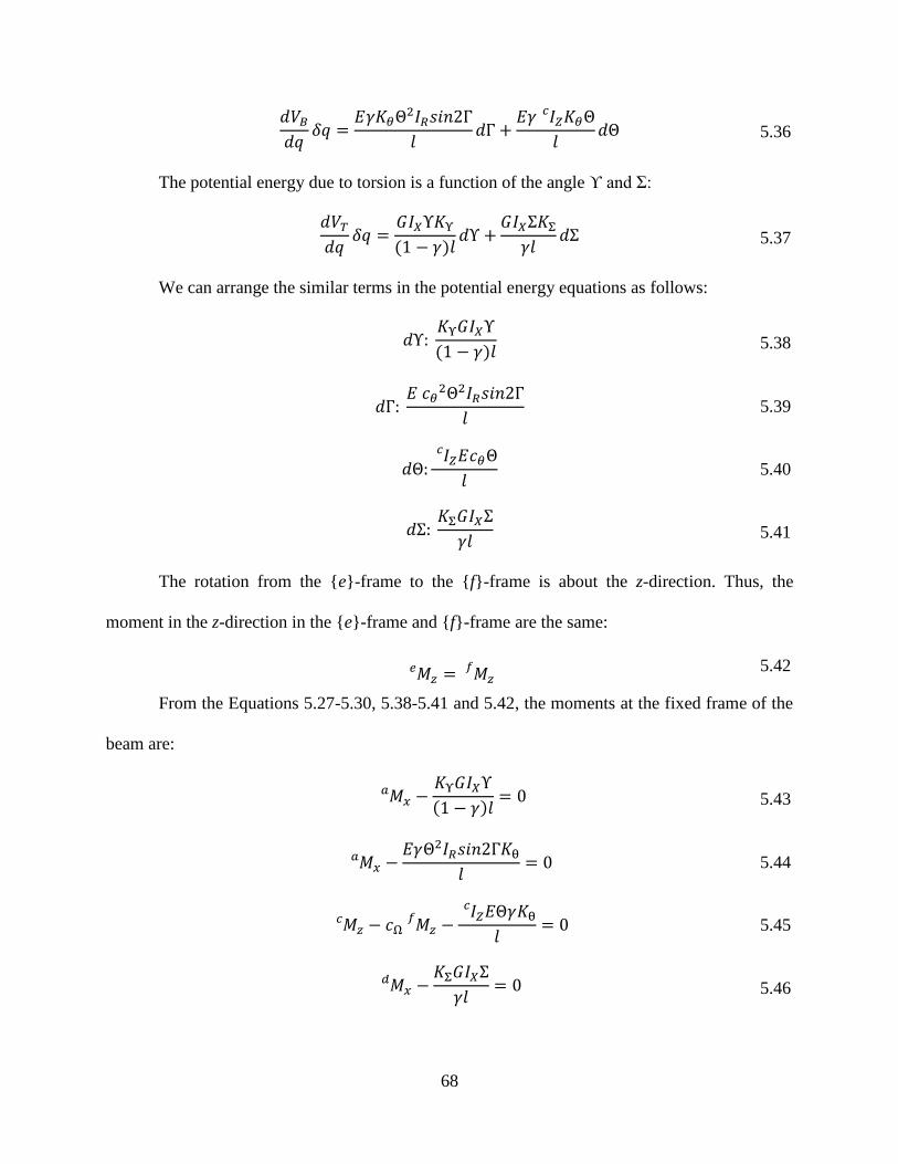
68

𝑑𝑉𝐵

𝑑𝑞𝛿𝑞 =

𝐸𝛾𝐾𝜃Θ2𝐼𝑅𝑠𝑖𝑛2Γ

𝑙𝑑Γ +

𝐸𝛾 𝐼𝑍𝑐 𝐾𝜃Θ

𝑙𝑑Θ 5.36

The potential energy due to torsion is a function of the angle ϒ and Σ:

𝑑𝑉𝑇

𝑑𝑞𝛿𝑞 =

𝐺𝐼𝑋Υ𝐾Υ

(1 − 𝛾)𝑙𝑑Υ +

𝐺𝐼𝑋Σ𝐾Σ

𝛾𝑙𝑑Σ 5.37

We can arrange the similar terms in the potential energy equations as follows:

𝑑Υ: 𝐾Υ𝐺𝐼𝑋Υ

(1 − 𝛾)𝑙 5.38

𝑑Γ: 𝐸 𝑐𝜃

2Θ2𝐼𝑅𝑠𝑖𝑛2Γ

𝑙 5.39

𝑑Θ:𝐼𝑍

𝑐 𝐸𝑐𝜃Θ

𝑙 5.40

𝑑Σ: 𝐾Σ𝐺𝐼𝑋Σ

𝛾𝑙 5.41

The rotation from the {e}-frame to the {f}-frame is about the z-direction. Thus, the

moment in the z-direction in the {e}-frame and {f}-frame are the same:

𝑀𝑧

𝑒 = 𝑀𝑧𝑓

5.42

From the Equations 5.27-5.30, 5.38-5.41 and 5.42, the moments at the fixed frame of the

beam are:

𝑀𝑥𝑎 −

𝐾Υ𝐺𝐼𝑋Υ

(1 − 𝛾)𝑙= 0 5.43

𝑀𝑥𝑎 −

𝐸𝛾Θ2𝐼𝑅𝑠𝑖𝑛2Γ𝐾θ

𝑙= 0 5.44

𝑀𝑧𝑐 − 𝑐Ω 𝑀𝑧

𝑓−

𝐼𝑍𝑐 𝐸Θ𝛾𝐾θ

𝑙= 0 5.45

𝑀𝑥𝑑 −

𝐾Σ𝐺𝐼𝑋Σ

𝛾𝑙= 0 5.46

69

Thus, using Equations 5.43-5.46 the PRBM parameters 𝛾, 𝐾Υ, 𝐾θ, 𝐾Σ and 𝑐Ω are known.

The deflection of a beam with parameters E, I, l subjected to a moment can be found.

5.3 Derivation of PRBM Parameters

In this section, the results from the differential equations and the virtual work are

combined to obtain the equations for the parameters of the PRBM. We expect these parameters

to be nearly constant across a large range of values allowing for Equations 5.43-5.46 to be used

to predict the beam’s motion. From the governing equations of the beam, the orientation of the

beam from the free to the fixed end of the beam is given by the Euler angles 𝜙, θ, and ψ. The

rotation can also be found with thru the set of kinematic variables , , , and . The

rotation of the free-end ({h}-frame) with respect to the fixed-end ({a}-frame) can be expressed

using the compliant beam data and the PRBM angles as:

𝑅𝑞ℎ ( 𝑥𝑞 , 𝜓 ) 𝑅𝑝

𝑞 ( 𝑧𝑝 , θ ) 𝑅𝑎𝑝 ( 𝑥𝑎 , 𝜙 )

= 𝑅𝑓ℎ ( 𝑥

𝑓, Φ) 𝑅𝑒

𝑓( 𝑧𝑒 , Ω) 𝑅𝑑

𝑒 ( 𝑥𝑑 , Σ) 𝑅𝑐𝑑 ( 𝑧𝑐 , Θ) 𝑅𝑎

𝑐 ( 𝑥𝑎 , Ψ)

5.47

The angles 𝜙, θ, and ψ are obtained from the governing equations of the beam. Thus, the

rotation angles Σ, Ω, and Φ can be expressed by:

𝑅ΣΩΦ = 𝑅𝑥(Σ) 𝑅𝑧(Ω) 𝑅𝑥(Φ) = 𝑅𝑧(Θ)−1 𝑅𝑥(Ψ)−1𝑅𝑥(𝜓) 𝑅𝑧(θ) 𝑅𝑥(𝜙) 5.48

The exact value of the angle Ψ is calculated by solving Equations 5.15 and 5.16, and

given by:

Ψ = acot (𝑏𝑠

𝑐𝑠⁄ ) 5.49

The values of the characteristic bend angle Θ and the characteristic radius factors are

found by solving Equations 5.14-5.16, such that the characteristic radius factor is:

70

γ =

(1 −𝑎𝑠

𝑙⁄ )2

+ (𝑏𝑠

𝑙⁄ )

2

+ (𝑐𝑠

𝑙⁄ )2

2(1 −𝑎𝑠

𝑙⁄ )2

5.50

Solving Equations 5.14 and 5.15, the characteristic bend angle is expressed by:

Θ = atan(𝑏𝑠

𝑎𝑠 + 𝑙(1 − 𝛾)⁄ ) 5.51

where as, bs, and cs is the position of the beam tip with respect to the x, y and z direction,

respectively. From the coefficients of the multiplication of Equation 5.48, the coefficients of Σ,

Ω and Φ angles are calculated as follows:

Ω = acos [𝑅ΣΩΦ(1,1)] 5.52

Φ = atan(𝑅𝛴𝛺𝛷(1,3)

𝑠𝑖𝑛(𝛺)

−𝑅𝛴𝛺𝛷(1,2)

𝑠𝑖𝑛(𝛺)⁄ ) 5.53

𝛴 = atan(𝑅𝛴𝛺𝛷(3,1)

𝑠𝑖𝑛(𝛺)

𝑅𝛴𝛺𝛷(2,1)

𝑠𝑖𝑛(𝛺)⁄ ) 5.54

Equations 5.52-5.54 are sufficient to solve for the angles Ω and Φ. To solve Equations

5.43-5.46, one can assume that:

𝑀𝑅 =𝐸𝛾𝐼𝑅Θ𝐾𝜃

𝑙 5.55

�� =

𝐸𝛾𝐼Θ𝐾𝜃

𝑙

5.56

Equations 5.44 and 5.45 become:

𝑀𝑥𝑎 − Θ𝑀𝑅𝑠𝑖𝑛2Γ = 0 5.57

𝑀𝑧𝑐 + 𝑐Ω 𝑀𝑧

𝑓− (M − 𝑀𝑅 cos 2Γ) = 0 5.58

Solving the Equations 5.57 and 5.58:

71

sin 2Γ =𝑀𝑥

𝑐

𝑀𝑅Θ 5.59

cos 2Γ =�� − ( 𝑀𝑧

𝑐 + 𝑐Ω 𝑀𝑧𝑓

)

𝑀𝑅 5.60

Using the trigonometric identity: sin2 2Γ + cos2 2Γ = 1, and because 𝑀𝑅 = �� (𝐼𝑅

𝐼),

Equations 5.59-5.60 can be combined into a quadratic formula of the form 𝐴��2 + 𝐵�� + 𝐶 = 0,

where:

𝐴: 1 − (𝐼𝑅

𝐼 )

2

5.61

𝐵: − 2( 𝑀𝑧𝑐 + 𝑐Ω 𝑀𝑧

𝑓) 5.62

𝐶: ( 𝑀𝑧

𝑑 + 𝑐Ω 𝑀𝑧𝑓

)2+ (

𝑀𝑥𝑎

Θ)

2

5.63

The quadratic formula can be solved using Matlab to calculate the value of ��. Knowing

the values of ��, the angle Γ can be obtained by dividing Equation 5.59 over Equation 5.60:

tan 2Γ =𝑀𝑥

𝑐

Θ[�� − ( 𝑀𝑧𝑐 + 𝑐Ω 𝑀𝑧

𝑓)]

5.64

The bending stiffness 𝐾θ can be calculated from Equation 5.56:

𝐾𝜃 =��𝑙

𝐸𝛾𝐼Θ 5.65

From Equation 5.46, the stiffness coefficient 𝐾Σ:

𝐾Σ =𝛾𝑙 𝑀𝑥

𝑑

𝐺𝐼𝑋Σ 5.66

Because Equations 5.43 and 5.44 contain the same moment 𝑀𝑥𝑎 , the stiffness coefficient

𝐾Υ can be found by equating the two equations and solving for 𝐾Υ:

𝐸𝛾Θ2𝐼𝑅𝑠𝑖𝑛2Γ𝐾θ

𝑙=

𝐾Υ𝐺𝐼𝑋Υ

(1 − 𝛾)𝑙

5.67

72

𝐾Υ =𝐸𝛾Θ2𝐼𝑅𝑠𝑖𝑛2Γ𝐾θ(1 − 𝛾)

𝐺𝐼𝑋Υ

5.68

5.4 Verification

The equations presented in the previous sections can be partially verified by showing that

they reduce to the equations of a planar beam under planar loading. For planar beams, the in-

plane moment (Mz) in the follower frame is equal to the moment as in the fixed frame. There is

no twist of the PRB or the straight beam, which means that the rotation angles in the x-direction

Φ, Σ and Ψ are equal to zero. The Euler angles ϕ and 𝜓 remain at 180 and -180 degrees thru the

length of the beam while the tip angle θ increases. The relationship between the beams tip angle

θ and the variables Θ and Ω is equal to:

θ = Ω + Θ 5.69

When an out-of-plane moment (My) is applied in the follower frame of the beam, the

straight part of the beam experiences a twist about the x-axis by the angle Ψ of 90 degrees,

followed by an angle Θ which rotates the PRB link in the y-axis. There will be no twisting of the

PRB link, which means that the angles Γ and Σ are equal to zero, but the angle at the beam tip

Φ= -ϒ= -Ψ, rotates the tip in the negative x-direction to reposition direction of the beam. The

relationship between the slope angle θ and the variables Θ and Ω is equal to Equation 5.69.

For a planar beam with an in-plane applied moment, the moments in the y and x-direction

are equal to zero, therefore, Equations 5.43, 5.44 and 5.46 are also equal to zero. The moment in

the z-direction remains the same through the beam, thereby, Equation 5.45 reduces to:

𝑀𝑧𝑐 = 𝑀𝑧

𝑓= 𝑀𝑧 5.70

Because no moments are applied in the y and x-direction, the stiffness parameter is:

𝑐Ω = 𝑐θ − 1 5.71

Because there is no twist along the beam, Γ=0. Thus, for a planar beam:

73

𝐼𝑍𝑍𝑐 = 𝐼𝑍𝑍 5.72

And from Chapter 4, Equation 4.33:

𝐾θ = 𝑐θ𝐾s 5.73

where 𝐾s is the spring constant. Applying Equations 5.70-5.73 into 5.45 reduces to:

𝑀𝑧 =𝛾𝐸𝐼𝑍𝐾s

𝑙Θ 5.74

For the axisymmetric beam, the moments of inertia with respect to the y and z directions

on the {a}-frame are equal. Therefore,

Because there is no rotation in the pseudo-rigid-body link, Σ=0, the moments in the {c}-

frame and the {f}-frame remain constant. Applying this, we have obtained the same derivation as

with the planar beam, validating the equations of the rectangular pseudo-rigid-body model.

5.5 Approximations of the PRBM Constants

The flow chart in Figure 5.4 shows the procedure to find the exact values of the PRBM

for a rectangular cantilever beam. The process can be divided in five parts: (1) an in-plane and

out-of-plane moment were applied in the follower frame (2) using the governing equations of the

beam, we obtain the displacement coordinates, curvature and the rotation of the beam for a given

aspect ratio with Equations 5.1-5.9 (3) find the rotation angles Σ, Ω and Φ from Equations 5.52-

5.54, (4) calculate the parametric angle coefficients 𝑐𝜃, 𝑐Ω from Equation 5.19 and the moment

vector at the different frames ( �� 𝑐 , �� 𝑑 , �� 𝑒 , �� 𝑓

) with the rotations obtained in step 3, (5)

calculate �� with Equations 5.61-5.63, (6) calculate the twist angles Γ and Υ with Equations 5.33

and 5.18, respectively and the stiffness parameters 𝐾𝜃, 𝐾Υ and 𝐾Σ from Equations 5.65, 5.66 and

5.68, respectively.

𝐼𝑍𝑐 = 𝐼𝑍 5.75

74

Figure 5.4. Flow chart with the process to derive the PRBM parameters.

With the exact values of the PRBM, this section presents the approximations of the

characteristic radius factor γ, the parametric angle coefficients 𝑐𝜃 and 𝑐Ω, the stiffness

coefficients 𝐾𝜃, 𝐾Υ, 𝐾Σ and the rotation angles Ψ, Θ, Σ, Ω, Φ, Γ and ϒ as a function of the aspect

ratio of the beam.

When the perturbation ratio is less than one, the angle between the in-plane and the out-

of-plane moment is less than 45 degrees. The process to obtain the PRBM parameters is similar

to the one in the preceding section, with the difference that the perturbation ratio was limited to

values ranging from 0.1 to 1.0.

Knowing: |M|, ε, υ, AR

From the governing equations of a beam:

𝜏𝑥, 𝜅𝑦, 𝜅𝑧 , 𝜙, 𝜃, 𝜓, 𝑎, 𝑏, 𝑐

Calculate: 𝛾, Θ,Ψ

Calculate: Σ, Ω,Φ

𝑐𝜃

Calculate: 𝑐𝜃, 𝑐Ω, �� 𝑐 , �� 𝑑 , �� 𝑒 , �� 𝑓

Calculate: ��, 𝐾𝜃

Calculate: Γ, Υ, 𝐾Υ,𝐾Σ

75

The moments in the fixed frame from rectangular ( 𝑀𝑎𝑥, 𝑀𝑎

𝑦, 𝑀𝑎𝑧) can be expressed in

spherical coordinates as [43]:

𝑀𝑎

𝑥 = |𝑀| sin 𝜂 sin 𝜉 5.76

𝑀𝑎

𝑦 = |𝑀| cos 𝜂 5.77

𝑀𝑎𝑧 = |𝑀| sin 𝜂 cos 𝜉 5.78

where |M| is the magnitude of the non-follower moment, 𝜉 is the azimuth angle (the angle of the

moment in the xz-plane) and, 𝜂 is the angle inclination angle (angle of the moment in the xy-

plane), as shown in Figure 5.5.

Figure 5.5. Angles of the applied moment in the fixed frame.

Because the angle of the moment changes with the perturbation ratio, we can obtain the

radius and the angle and find the location where the maximum coordinates are valid. The angle

of the moment in the non-follower frame 𝜉 and 𝜂 can be used to obtain the limits where the

PRBM parameters are valid.

For example, a moment in the follower frame 𝑀ℎ𝑧 and a perturbed moment of 𝑀ℎ

𝑦 =

휀 𝑀ℎ𝑧 was applied to the beam with a cross section of 2.5. Using the governing equations of the

beam, the Euler angles 𝜙, 𝜃 and 𝜓 are found. The moments in the fixed frame ( �� 𝑎 ) is found by

η

ξ

76

multiplying the moment in the follower frame ( 𝑀ℎ𝑧) by the XZX matrix of Euler rotations 𝑅ℎ

𝑎

such as:

�� 𝑎 = 𝑅𝑝𝑎 ( 𝑥𝑎 , 𝜙) 𝑅𝑞

𝑝 ( 𝑧𝑝 , θ) 𝑅ℎ𝑞 ( 𝑥𝑞 , 𝜓) �� ℎ 5.79

From Equations 5.76-5.78, the inclination and azimuth angle (η and ξ, respectively) of

the moment in the fixed frame are:

𝜉 = atan(

𝑀𝑎𝑥

𝑀𝑎𝑧) 5.80

𝜂 = acos (

𝑀𝑎𝑦

|𝑀|) 5.81

As shown in Figure 5.6, the simplified parameters are not valid in the entire area of the

quadrant. We can approximate the area that covers the applied moments with a radius (ρ) and an

angle (Λ). Figure 5.6 shows the area where the perturbation factor is less than one for the 2.5

aspect ratio as a function of the angles at the fixed frame 𝜉 and 𝜂. For this case, the radius would

be the distance between point A and point B in the figure and the angle Λ is the angle between

the horizontal and the point A. With this information, we can obtain the maximum inclination

and azimuth angle (η and ξ, respectively) where the model is valid.

Table 5.1 contains the limit area of the simplified PRBM parameters for different aspect

ratios when non-follower moments are applied to the cantilever beam. When the aspect ratio is

higher than 2.75, the simplification is valid for the entire quadrant.

The maximum inclination and azimuth angle (η and ξ, respectively) for the aspect ratios

presented in Table 5.1 are calculated as:

𝜉𝑚𝑎𝑥 = 𝜌 sin Λ + 𝜋/2 5.82

𝜂𝑚𝑎𝑥 = 𝜌 cosΛ 5.83

The approximation of the PRBM parameters for perturbation ratios less than 1 is below.

The maximum tip slope angle for the approximation is 120 degrees.

77

Figure 5.6. Perturbation ratio as a function of the angles of the applied moment 𝜉 and 𝜂 for the

2.5 aspect ratio.

Table 5.1. Limits of the PRBM parameters for different aspect ratios.

AR ρ Λ (radians)

1.25 0.97 0.79

1.50 1.02 1.02

1.75 0.99 1.16

2.00 0.92 1.29

2.25 0.87 1.39

2.50 0.83 1.52

2.75 0.80 1.57

1.5 1.6 1.7 1.8 1.9 2 2.1 2.2 2.3 2.40

0.2

0.4

0.6

0.8

1

(radians)

(

radia

ns)

0.1

0.2

0.3

0.4

0.5

0.6

0.7

0.8

0.9

1

A

B

78

5.5.1 Approximation of the Characteristic Radius Factor

The characteristic radius factor gives the location of the pseudo-rigid-body model joint.

The exact values of the angles Ψ and ϴ where calculated from Equations 5.49 and 5.51,

respectively with the theoretical coordinates of the beam. The exact value of the characteristic

radius was calculated from Equation 5.50.

Figure 5.7 shows the relationship between the exact characteristic radius, as a function of

the angle θ, ϕ and the beam aspect ratio ranging from 1.25 to 4. The plot shows the exact

characteristic radius factor for the different aspect ratios. As shown in the plot, the relationship

between the characteristic radius and the aspect ratio depend on the tip angle θ.

Figure 5.7. Exact values of the characteristic radius factor, γ, as a function of the tip angles ϕ and

θ and the beam aspect ratio.

Table 5.2 contains the approximated values of the characteristic radius factor. The

average of the characteristic radius factor was calculated with the exact values of the PRB angles

Θ and Ψ. With the theoretical values of the tip location (at, bt and ct), we are able to calculate the

79

relative deflection error. The relative deflection error estimates the difference between the

theoretical and the approximated tip location, where the maximum relative deflection error is

6%. The maximum error of the approximated characteristic radius factor is along the horizontal

axis (x-direction) of the beam.

Table 5.2. Approximated values of the characteristic radius factor as a function of the aspect

ratio of the beam.

AR γ Std.

Dev. γ

Relative

error (%)

Max. error

a (%)

Max. error

b (%)

Max. error

c (%)

1.00 0.7432 0.0056 1.617 2.119 0.898 0.898

1.25 0.7401 0.0086 3.499 4.479 1.294 1.294

1.50 0.7358 0.0137 6.653 7.967 1.870 1.870

1.75 0.7354 0.0140 6.590 7.835 1.921 1.921

2.00 0.7365 0.0124 5.664 6.448 1.772 1.772

2.25 0.7378 0.0107 4.676 5.291 1.600 1.600

2.50 0.7389 0.0094 3.898 4.913 1.460 1.460

2.75 0.7398 0.0085 3.351 4.280 1.345 1.345

3.00 0.7404 0.0078 2.968 3.757 1.266 1.266

3.25 0.7409 0.0073 2.715 3.431 1.192 1.192

3.50 0.7413 0.0070 2.527 3.333 1.146 1.146

3.75 0.7415 0.0068 2.389 3.262 1.114 1.114

4.00 0.7417 0.0066 2.208 2.928 1.084 1.084

In the approximation of the characteristic radius factor, the maximum error comes from

the horizontal deflection (a). The approximated characteristic radius factor over estimates the

horizontal deflection. Figure 5.8 presents the difference between the theoretical and

approximated horizontal deflection for a beam with aspect ratio equal to 2. The red points

represent the theoretical deflection and the blue squares the approximated deflections. The error

occurs at tip angles over 100 degrees. The cause of the discrepancy in the theoretical and

80

approximated values is because for the horizontal deflection we are only taking in consideration

the PRB angle Θ and not the out of plane angle Ψ. The vertical and out-of-plane deflection

maximum error are the same, which are less than 2%, where the maximum error occurs at lower

aspect ratios.

Figure 5.8. Theoretical and approximated horizontal deflections versus tip angles for aspect ratio

equal to 2.

5.5.2 Approximation of the Parametric Angle Coefficients

The bending parametric angle coefficient is the ratio of the tip angle to the bending PRB

angle Θ.

𝑐𝜃 = 𝜃/Θ 5.84

Figure 5.9 presents the exact values of the bending parametric angle coefficient (𝑐𝜃), as a

function of the tip angle θ for aspect ratios ranging from 1.25 to 5.0. The parametric angle ranges

from 1.47 to 1.56, as shown in the figure. A linear regression routine was used to obtain the

approximated bending parametric angle coefficient given the exact values of the tip angle θ and

0 20 40 60 80 100 1200.4

0.5

0.6

0.7

0.8

0.9

1

(deg)

as/l

81

the PRB link angle Θ for tip slope angles less than 120 degrees. Table 5.3 presents the

approximated bending parametric angle coefficients for different aspect ratios.

Figure 5.9. Exact values of the parametric angle coefficient, cθ, as a function of the tip angles θ

for aspect ratios ranging from 1.25 to 4.

The function of the approximated bending parametric angle coefficient (cθa) in the PRBM

is to calculate the PRB angle Θ. The error between the exact and approximated angle Θ is

defined as:

𝑒𝑟𝑟𝑜𝑟 (Θ) =Θ − Θ𝑎

Θ∗ 100 5.85

where Θ𝑎 = 𝜃0/𝑐𝜃𝑎. Table 5.3 presents the approximated bending parametric angle coefficients

and the percentage error the PRB angle Θ as a function of the aspect ratio. The maximum error

found between the approximated and exact PRB angle Θ is 1.24%.

From Equation 5.19, the PRB-link parametric angle coefficient is the ratio of the tip angle

to the bending PRB angle Θ and the rotation angle Ω:

82

𝑐Ω = Ω/Θ 5.86

Table 5.3. Approximated values of the bending parametric angle coefficient (cθ) as a function of

the aspect ratio of the beam.

AR cθa R2 cθa Max. error Θ𝑎(%)

1.00 1.5150 0.9999 0.978

1.25 1.5178 0.9999 1.160

1.50 1.5191 0.9999 1.240

1.75 1.5184 0.9999 1.197

2.00 1.5182 0.9999 1.181

2.25 1.5183 0.9999 1.187

2.50 1.5183 0.9999 1.188

2.75 1.5183 0.9999 1.189

3.00 1.5182 0.9999 1.185

3.25 1.5180 0.9999 1.169

3.50 1.5178 0.9999 1.161

3.75 1.5178 0.9999 1.156

4.00 1.5176 0.9999 1.146

Figure 5.9 presents the exact values of the PRB-link parametric angle coefficient 𝑐Ω, as a

function of the tip angles ϕ and θ for aspect ratios ranging from 1.25 to 4.0. The exact values of

cΩ ranges from 0.5 to 0.56 for tip angles ranging from 0-120 degrees, and increases to 0.59 for

higher tip angles. A linear regression routine was used to find the approximated relationship

between the tip angle and the PRB-link angle for tip slope angles less than 120 degrees. Table

5.4 presents the approximated values of the PRB link parametric angle coefficient 𝑐Ω for

different aspect ratios.

The error associated with the Ω angle can be found thru:

𝑒𝑟𝑟𝑜𝑟 (Ω) =Ω − Ω𝑎

Ω∗ 100 5.87

83

where Ω𝑎 = 𝑐𝛺Θ𝑎. As shown in Table 5.4, the error of the approximated Ω can be 10% for low

aspect ratios. The error in the approximated angle Ω is higher because Ω𝑎 depends on the values

of the approximated angle Θ𝑎. The error is also higher at low aspect ratios because there is an

increase in the torsion of the PRB link given by the angle Σ.

Figure 5.10. Exact values of the PRB-link parametric angle coefficient, cΩ, as a function of the

tip angles ϕ and θ.

Because the angles Ω and Θ depend on 𝑐θ, the rotation angle Ω can be calculated as:

Ω = (𝑐θa − 1)Θ 5.88

We can also assume that the angles Ψ and Φ are linearly related as:

Ψ = 𝑐ΨΦ 5.89

Figure 5.11 presents the exact value of the parametric angle coefficient 𝑐Ψ as a function

of the aspect ratio of the beams cross-section and the tip angles ϕ and θ.

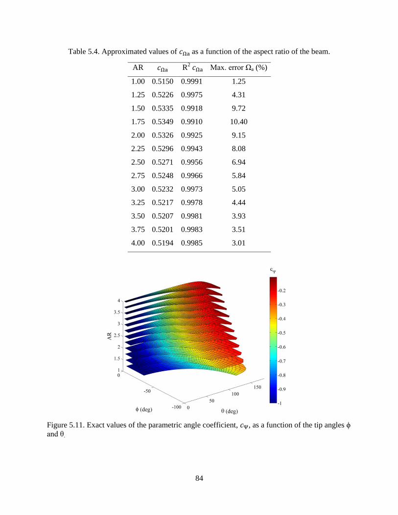
84

Table 5.4. Approximated values of 𝑐Ωa as a function of the aspect ratio of the beam.

AR 𝑐Ωa R2 𝑐Ωa Max. error Ωa (%)

1.00 0.5150 0.9991 1.25

1.25 0.5226 0.9975 4.31

1.50 0.5335 0.9918 9.72

1.75 0.5349 0.9910 10.40

2.00 0.5326 0.9925 9.15

2.25 0.5296 0.9943 8.08

2.50 0.5271 0.9956 6.94

2.75 0.5248 0.9966 5.84

3.00 0.5232 0.9973 5.05

3.25 0.5217 0.9978 4.44

3.50 0.5207 0.9981 3.93

3.75 0.5201 0.9983 3.51

4.00 0.5194 0.9985 3.01

Figure 5.11. Exact values of the parametric angle coefficient, 𝑐Ψ, as a function of the tip angles ϕ

and θ.

85

An approximated value of the parametric angle coefficient 𝑐Ψ can be found as a function

of the tip angles θ and ϕ as shown in Figure 5.11. For tip angles θ less than 120 degrees, 𝑐Ψ

varies from -1.0 to -0.4.

5.5.3 Approximation of the Stiffness Coefficients

For the approximation of stiffness coefficients, a series of loads where applied to the free-

end of the beam ({h}-frame), which caused a maximum tip slope which ranged from 0 to 120°.

To this loads, a perturbed out-of-plane moment in the Y-direction was applied at the end for

different aspect ratios. The moments at the different frames were calculated using the coordinate

transformations.

The bending stiffness coefficient 𝐾θ was calculated from Equation 5.65. Figure 5.12

presents the bending stiffness coefficient 𝐾θ as a function of the tip angles θ and ϕ. The bending

stiffness coefficient ranges from 2.03 to 2.3. Table 5.5 presents the approximate the bending

stiffness coefficient for each aspect ratio. The mean and the standard deviation for each aspect

ratio was calculated to approximate 𝐾θ.

Figure 5.12. Bending stiffness coefficient Kθ as a function of the tip angles ϕ and θ.

86

Table 5.5. Approximated values of the bending stiffness coefficient Kθ and the standard

deviation as a function of the aspect ratio of the beam.

AR Kθa Std. Dev. Kθ

1.00 2.0306 0.0254

1.25 2.0415 0.0343

1.50 2.0553 0.0476

1.75 2.0570 0.0497

2.00 2.0518 0.0428

2.25 2.0460 0.0358

2.50 2.0415 0.0310

2.75 2.0383 0.0278

3.00 2.0362 0.0261

3.25 2.0344 0.0248

3.50 2.0334 0.0243

3.75 2.0329 0.0240

4.00 2.0324 0.0239

The torsion of the beam is a function of the ϒ and Σ angles. Where ϒ is the deformation

at the fixed end of the beam and Σ is the rotation of the pseudo-rigid link. From Equation 5.68,

the stiffness coefficient 𝐾Υ:

𝐾Υ =𝛾 (1 − 𝛾)𝐾𝜃Θ2sin (2Γ)(1 + 𝜐)(𝐴𝑅2 − 1)

Υ(𝐴𝑅2 + 1) 5.90

Figure 5.13 shows the stiffness coefficient 𝐾Υ as a function of the tip angles ϕ and θ.

From the fixed frame {a}, the first rotation is about the Υ-angle. 𝑀𝑥𝑎 is the first rotation about

the x-frame, the moment in the x-frame is the same. The stiffness coefficient 𝐾Υ is a measure of

resistance to deformation on the straight part of the beam.

87

Figure 5.13. Stiffness parameter Kϒ as a function of the tip angles ϕ and θ.

The mean and the standard deviation for each aspect ratio were calculated to approximate

Kϒ. Table 5.6 presents the approximate the bending stiffness coefficient for each aspect ratio.

The stiffness coefficient 𝐾Σ can be calculated from Equation 5.66, such as:

𝐾Σ =𝛾𝑙 𝑀𝑥

𝑑

𝐺𝐼𝑋Σ 5.91

The rotation of the angle Σ, there is a rotation about the Ψ-angle around the x-axis and a

Θ-rotation about the z-axis. We can find the stiffness coefficient is a function of the aspect ratio

of the beam and the tip angles θ and ϕ, as shown in Figure 5.14.

As shown in Figure 5.14, for aspect ratios higher than 3.0, 𝐾Σ is approximately 0.75. For

lower aspect ratios, the torsion stiffness coefficient is a function of the aspect ratio and the tip

angles θ and ϕ. The mean and the standard deviation of the torsion stiffness coefficient are

presented in Table 5.7.

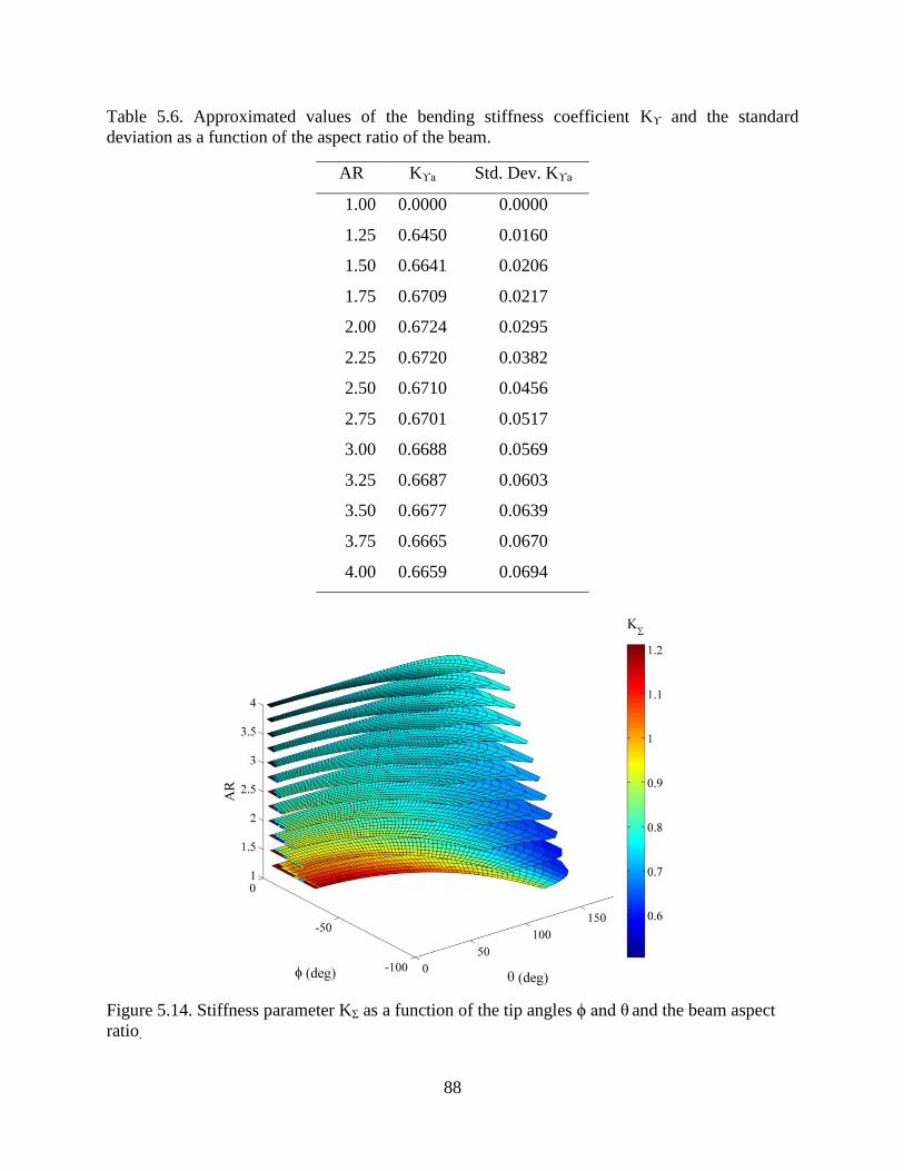
88

Table 5.6. Approximated values of the bending stiffness coefficient Kϒ and the standard

deviation as a function of the aspect ratio of the beam.

AR Kϒa Std. Dev. Kϒa

1.00 0.0000 0.0000

1.25 0.6450 0.0160

1.50 0.6641 0.0206

1.75 0.6709 0.0217

2.00 0.6724 0.0295

2.25 0.6720 0.0382

2.50 0.6710 0.0456

2.75 0.6701 0.0517

3.00 0.6688 0.0569

3.25 0.6687 0.0603

3.50 0.6677 0.0639

3.75 0.6665 0.0670

4.00 0.6659 0.0694

Figure 5.14. Stiffness parameter KΣ as a function of the tip angles ϕ and θ and the beam aspect

ratio.

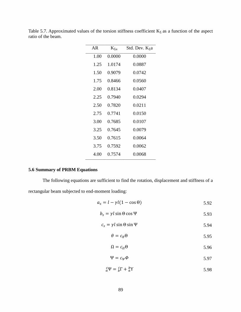
89

Table 5.7. Approximated values of the torsion stiffness coefficient KΣ as a function of the aspect

ratio of the beam.

5.6 Summary of PRBM Equations

The following equations are sufficient to find the rotation, displacement and stiffness of a

rectangular beam subjected to end-moment loading:

𝑎𝑠 = 𝑙 − 𝛾𝑙(1 − cosΘ) 5.92


𝑐𝑠 = 𝛾𝑙 sin Θ sinΨ 5.94

𝜃 = 𝑐𝜃Θ 5.95

Ω = 𝑐𝛺Θ 5.96

Ψ = 𝑐𝛹𝛷 5.97

Ψ𝑎𝑐 = Γ𝑏

𝑐 + Υ𝑎𝑏 5.98

AR KΣa Std. Dev. KΣa

1.00 0.0000 0.0000

1.25 1.0174 0.0887

1.50 0.9079 0.0742

1.75 0.8466 0.0560

2.00 0.8134 0.0407

2.25 0.7940 0.0294

2.50 0.7820 0.0211

2.75 0.7741 0.0150

3.00 0.7685 0.0107

3.25 0.7645 0.0079

3.50 0.7615 0.0064

3.75 0.7592 0.0062

4.00 0.7574 0.0068

90

𝑀𝑥𝑎 −

𝐾𝛶𝐺𝐼𝑋Υ

(1 − 𝛾)𝑙= 0 5.99

𝑀𝑥

𝑎 −𝐸𝛾Θ2𝐼𝑅𝑠𝑖𝑛2Γ𝐾𝜃

𝑙= 0 5.100

𝑀𝑧

𝑐 − 𝑐𝛺 𝑀𝑧𝑓

−𝐼𝑍

𝑐 𝐸Θ𝛾𝐾𝜃

𝑙= 0 5.101

𝑀𝑥

𝑑 −𝐾𝛴𝐺𝐼𝑋Σ

𝛾𝑙= 0 5.102

Knowing the aspect ratio of the beams cross section (the ratio of the width of the beam

over the height of the beam) we can obtain the approximation of the PRBM parameters

𝛾, 𝑐Ω, 𝑐θ, 𝑐Ψ, 𝐾Υ, 𝐾θ and 𝐾Σ from section 5.5. Equations 5.92- 5.102 can be added into Matlab to

solve for the other parameters.

5.7 Conclusion

The pseudo-rigid-body model for a beam of rectangular cross-section consists of two

rigid links connected by a spherical joint and a spherical cap. The spherical cap was added to

describe the orientation of the beams tip. The deflection of the beam’s tip is found by

substituting the PRB parameters in Equations 5.14-5.16.

Perturbation theory was used to apply the out-of-plane moment (My) in the follower

frame such that it ensures the applied load does not produce excessive out-of-plane deflection.

The limits of the PRBM parameters which contain a relative deflection error of 6.0% for selected

aspect ratios and perturbation factors less than one were described. The PRBM parameters

𝛾, 𝑐Ω, 𝑐θ, 𝑐Ψ, 𝐾Υ, 𝐾θ and 𝐾Σ depend on the aspect ratio of the beam. Tables with the

approximations of the PRBM parameters as a function of the aspect ratio are included in this

Chapter.

91

Chapter 6

Conclusions and Recommendations

The objective of this study was to describe kinematic models (Pseudo-Rigid-Body

Models) for approximating large-deflection of spatial cantilever beams that undergo multiple

bending motions thru end-moment loading. PRBMs for axisymmetric and rectangular cross-

section spatial beams with moment-loading were developed in this dissertation.

The governing equations of a cantilever beam that undergoes large deflection due to force

and moment loading where developed and validated. These non-linear kinematic equations for a

cantilever beam contains the curvature, location and rotation of the beam. The resulting

deflections, curvatures and angles where used to developed a spatial Pseudo-Rigid-Body Model.

The pseudo-rigid-body model for an axisymmetric beam consists of two links connected

thru a spherical joint. It was found that the coordinates of the deflection of an axisymmetric

beam can be found by using the planar PRBM multiplied by a rotation in the x-direction. The

characteristic radius factor and the PRB angle coefficient for a beam with a single moment

applied at the end were optimized to minimize the error incurred using the deflection formulas of

the PRBM. This approximation provides an improvement to previous published parameters,

providing a relative error of 0.5% at a tip slope angle to 169.76 degrees.

The pseudo-rigid-body model for a beam of rectangular cross-section consists of two

rigid links connected by a spherical joint and a spherical cap. The spherical cap was added to

describe the orientation of the beam. The PRB parameters 𝛾, 𝑐Ω, 𝑐θ, 𝑐Ψ, 𝐾Υ, 𝐾θ and 𝐾Σ depend on

92

the aspect ratio (the ratio of the beams width over the height) of the beam. Tables with

approximations of the PRBM parameters as a function of the aspect ratio are included in Chapter

5.

6.1 Recommendations for Future Work

1. It was found that for a rectangular cantilever beam with multiple loading moments, the PRB-

link undergoes torsion. Another approach to model this torsion would be to develop a PRBM

consisting of 3 links connected thru 2 revolute joints to model the torsion of the longer PRB-

link.

2. Most of the error of the characteristic radius factor is from the horizontal deflection of the

beam. This error may be minimized by assuming that the total length of the PRBM is less

than the length of the straight beam.

3. A spatial PRBM with combined forces and moments will be the next step of this work.

93

References

[1] Frecker MI, Powell KM, Haluck R. Design of a Multifunctional Compliant Instrument for

Minimally Invasive Surgery. J.Biomech.Eng. 2005; 127: 990-993

[2] Gu D, Zhou Y. An approach to the capsule endoscopic robot with active drive motion.

Journal of Zhejiang University. 2011; 12: 223-231

[3] Yung-Lien W. Modular design process for a micro motion actuator. Mechatronics. 2005; 15:

793-806

[4] Bandopadhya D. Quasi-Static Tip Positioning of Multi-Segmented IPMC for Micro-

Manipulation following Euler-Bernoulli and Pseudo-Rigid Body Model. Journal of Reinforced

Plastics and Composites: 743

[5] Zubir MNM, Shirinzadeh B, Tian Y. A new design of piezoelectric driven compliant-based

microgripper for micromanipulation. Mechanism and Machine Theory. 2009; 44: 2248-2264

[6] Kennedy JA, Howell LL, Greenwood W. Compliant high-precision E-quintet ratcheting

(CHEQR) mechanism for safety and arming devices. Precision Engineering. 2007; 31: 13-21

[7] Frisch-Fay R. Flexible bars. Washington, D.C.: Butterworths. 1962

[8] Howell LL. Compliant mechanisms. New York: Wiley. 2001

[9] Aguirre ME, Frecker M. Design Innovation Size and Shape Optimization of a 1.0 mm

Multifunctional Forceps-Scissors Surgical Instrument. Journal of Medical Devices March, 2008;

2: 015001

[10] Cronin JA, Frecker IMI, Mathew A. Design of a Compliant Endoscopic Suturing

Instrument. J.Med.Devices. 2008; 2: 025002

[11] Zoppi M, Sieklicki W, Molfino R. Design of a Microrobotic Wrist for Needle Laparoscopic

Surgery. J.Mech.Des. 2008; 130: 102306

[12] Vitellaro G, L'Episcopo G, Trigona C, Ando B, Baglio S. A Compliant MEMS Device for

Out-of-Plane Displacements with Thermo-Electric Actuation. Journal of Microelectromechanical

Systems. 2014; 23: 661-671

94

[13] Sonmez U. Compliant MEMS Crash Sensor Designs: The Preliminary Simulation Results.

Intelligent Vehicles Symposium. IEEE 2007: 303-308

[14] Kota S, Joo J, Li Z, Rodgers S. M, Sniegowksi, J. Design of Compliant Mechanisms:

Applications to MEMS. Analog Integrated Circuits and Signal Processing. 2001; 29: 7-16

[15] Landon S. Development of Deployable Wings for Small Unmanned Aerial Vehicles Using

Compliant Mechanisms. 2007

[16] Kota S, Hetrick JA, Osborn R, Paul D, Pendleton E, Flick P, Tilmann C. Design and

application of compliant mechanisms for morphing aircraft structures. 2003: 24-33

[17] Khataita JP, Mukherjeeb S, Sethc B. Compliant design for flapping mechanism: A

minimum torque approach. Mechanism and Machine Theory: 3

[18] Yao-Wei Chin, Gih-Keong Lau. “Clicking” compliant mechanism for flapping-wing micro

aerial vehicle. Intelligent Robots and Systems (IROS), 2012 IEEE/RSJ International Conference

on 2012: 126-131

[19] Allred TM. Compliant mechanism suspensions. 2003

[20] Bisshopp KE, Drucker DC. Large Deflection of Cantilever Beams. Quarterly of applied

Math. 1945; 3: 272-275

[21] Sigmund O. On the design of compliant mechanisms using topology optimization.

Mechanics of structures and machines. 1997; 25: 493

[22] Howell LL, Magleby SP, Olsen BM. Handbook of compliant mechanisms. Chichester, West

Sussex, United Kingdom: John Wiley & Sons, Ltd, 2013

[23] Zhang A, Chen G. A Comprehensive Elliptic Integral Solution to the Large Deflection

Problems of Thin Beams in Compliant Mechanisms. Journal of Mechanisms and Robotics. 2013;

5: 021006

[24] Chen, G., and Zhang, A. Accuracy Evaluation of PRBM for Predicting Kinetostatic

Behavior of Flexible Segments in Compliant Mechanisms. Proceedings of the ASME 2011

International Design Engineering Technical Conferences and Computers and Information in

Engineering Conference. 2011

[25] Rao SS. Engineering Optimization: Theory and Practice, Fourth Edition. Hoboken, NJ,

USA: John Wiley & Sons, Inc. 2009

[26] Arora JS. Optimization of structural and mechanical systems. Hackensack, NJ: World

Scientific. 2007

95

[27] Sigmund O. On the Design of Compliant Mechanisms using Topology Optimization.

Mechanics of Structures and Machines. 1997; 25: 493

[28] Lee E, Gea HC. A strain based topology optimization method for compliant mechanism

design. Structural and Multidisciplinary Optimization. 2014; 49: 199-207

[29] Pedersen CBW, Buhl T, Sigmund O. Topology synthesis of large-displacement compliant

mechanisms. International Journal for Numerical Methods in Engineering. 2001; 50: 2683-2705

[30] Stanford B, Beran P. Conceptual Design of Compliant Mechanisms for Flapping Wings

with Topology Optimization. AIAA Journal. 2011; 49: 855-867

[31] Howell LL, Midha A. Parametric Deflection Approximations for End-Loaded, Large-

Deflection Beams in Compliant Mechanisms. Journal of Mechanical Design. 1995; 117: 156-165

[32] Howell LL, Midha A, Norton TW. Evaluation of Equivalent Spring Stiffness for Use in a

Pseudo-Rigid-Body Model of Large-Deflection Compliant Mechanisms. Journal of Mechanical

Design. 1996; 118: 126-131

[33] Pauly J, Midha A. Improved Pseudo-Rigid-Body Model Parameter Values for End-Force-

Loaded Compliant Beams. ASME Conference Proceedings 2004; 2004: 1513-1517

[34] M.H. D. Variable parametric pseudo-rigid-body model for large-deflection beams with end

loads. International Journal of Non-Linear Mechanics. 2001; 36: 1123-1133

[35] Feng Z, Yu Y, Wang W. Modeling of large-deflection links for compliant mechanisms.

Frontiers of Mechanical Engineering in China. 2010; 5: 294-301

[36] Yang XS. Applied Engineering Mathematics

[37] Su H. A Pseudo-Rigid-Body 3R Model for Determining Large Deflection of Cantilever

Beams Subject to Tip Loads. Journal of Mechanisms and Robotics. 2009; 1: 021008

[38] Wittwer JW. Robust Design and Model Validation of Nonlinear Compliant

Micromechanisms. Journal of microelectromechanical systems. 2006; 15: 33

[39] Chorlton F. Vector & tensor methods. Chichester, Eng.; New York: E. Horwood Ltd;

Halsted Press. 1976

[40] Axisa F, Trompette P. Modelling of Mechanical Systems [electronic resource]: Structural

Elements: Oxford: Elsevier Science & Technology, 2005. 2005

[41] LeBlanc DC. Statistics: concepts and applications for science / David C. LeBlanc: Sudbury,

MA : Jones and Bartlett. 2004

96

[42] Bender CM, Orszag SA. Advanced mathematical methods for scientists and engineers. 1,

Asymptotic methods and perturbation theory. Carl M. Bender, Steven A. Orszag. New York:

Springer. 1999

[43] Spiegel MR, Lipschutz S, Liu J. Mathematical Handbook of Formulas and Tables. New

York: McGraw-Hill. 2009

[44] Ramirez IA, Lusk CP. Spatial-Beam Large-Deflection Equations and Pseudo-Rigid-Body

Model for Axisymmetric Cantilever Beams. Proceedings of the ASME International Design

Engineering Technical Conferences, August 28-31, 2011

97

Appendices

98

Appendix A. Copyright Clearance

The following permission is for use of material in Chapter 3 and Chapter 4.

On Fri, Nov 21, 2014 at 12:24 PM, Philip DiVietro <[email protected]> wrote: Dear Ms. Ramirez, To confirm our conversation, you indeed have permission as stated in your request. There is no charge to you for this permission. Regarding, IDETC 2011 Conference Paper 47389, Spatial-Beam Large-Deflection Equations and Pseudo-Rigid-Body Model for Axisymmetric Cantilever Beams, by Issa A. Ramirez and Craig P. Lusk, pages 43-49, as published by ASME, 2011. Thank you for your support of ASME. Sincerely, Philip DiVietro

Philip V. DiVietro Managing Director, Publishing ASME 2 Park Avenue, 6th Floor New York, NY 10016-5990 Tel 1.212.591.7696 Mobile 1.631.553.1088 [email protected]

From: Issa Ramirez Rivera [mailto:[email protected]] Sent: Friday, November 21, 2014 12:17 PM To: Philip DiVietro Subject: Fwd: Permission request for dissertation

---------- Forwarded message ----------

From: Issa Ramirez Rivera <[email protected]>

Date: Mon, Nov 17, 2014 at 8:44 AM

Subject: Permission request for dissertation

To: [email protected]

Cc: Issa Ramirez <[email protected]>

Good morning,

I am one of the authors of the IDETC 2011 Conference Paper 47389. In the attachment is the filled

permissions request form to add parts of the conference paper as part of my dissertation.

If you have any questions, please let me know.

Thank you,

Issa A Ramirez


tel:1.212.591.7696

tel:1.631.553.1088






99

Appendix B. Matlab M-file

This Matlab code contains the main algorithm to obtain the curvatures, displacements and

rotations of a beam with moment-loading.

function moment_only_master

clc;clear all;close all

b=.04;e_p=1;

lb=10;h=.0100; AR=b/h;

Iy=(h*b^3)/12; Iz=(b*h^3)/12; Ix=Iy+Iz; ae=1; s=[0:lb]; x=s; y=0; z=0; %initial coordinates of the undeformed free end E=2.00000000E+11; %Young's Modulus v_p=.300; G=E/(2*(1+v_p)); AI=G*Ix; BI=E*Iy; CI=E*Iz;

%% Moments at the free-end theta_input=120*pi/180; MZ=(theta_input*E*Iz)/(lb);MX=0;MY=-e_p*MZ;

%% initial conditions at the deformed frame (X Y Z) at the end of the beam psi=0; theta=.0000000001; phi=0; dX=0; dY=0; dZ=0; kx_0=MX/(G*Ix); ky_0=MY/(E*Iy); kz_0=MZ/(E*Iz); K_input=[kx_0;ky_0;kz_0] y0=[psi theta phi kx_0 ky_0 kz_0 dX dY dZ] ; length_scale=[0:-lb/21:-lb];

[s_lenght,r]=ode45(@straight2,length_scale,y0);

function ds_out=straight2(s,y0);

si=y0(1); theta=y0(2); phi=y0(3);tx=y0(4); ky=y0(5); kz=y0(6);

dpsi=-ky*(cos(phi)/sin(theta))+kz*(sin(phi)/sin(theta)); dtheta=ky*sin(phi)+kz*cos(phi); dphi=tx+ky*cos(phi)*(cos(theta)/sin(theta))-

kz*sin(phi)*(cos(theta)/sin(theta));

F_dky=0;F_dkz=0;

dtx=(1/AI)*(((BI-CI)*ky*kz)+ 0); dky=(1/BI)*(((CI-AI)*kz*tx)+F_dky); dkz=(1/CI)*(((AI-BI)*tx*ky)+F_dkz);

dx_ds=cos(theta); dy_ds=cos(si)*sin(theta);

100

dz_ds=sin(si)*sin(theta);

ds_out=[dpsi dtheta dphi dtx dky dkz dx_ds dy_ds dz_ds]'; end

%% seen from the H-frame to the fixed frame A r(end,:);

AA=r(:,7); BB=r(:,8);CC=r(:,9);psi=r(:,1);theta=r(:,2);phi=r(:,3);

si=r(:,1)-r(1,1); theta=r(:,2)-r(1,2); phi=r(:,3)-r(1,3); kx=r(end,4);ky=r(end,5);kz=r(end,6);

kxyz_d=[r(end,4);r(end,5);r(end,6)] end_angles_XYZ=[si(end),theta(end),phi(end)]

%% change of frames: seen from the fixed (A) to the moving frame (H) for ii=1:1:length(theta);

R_qh= [1 0 0; 0 cos(phi(ii)) sin(phi(ii)); 0 -sin(phi(ii)) cos(phi(ii))]; R_pq=[cos(theta(ii)) sin(theta(ii)) 0;-sin(theta(ii)) cos(theta(ii)) 0; 0 0

1]; R_ap= [1 0 0; 0 cos(si(ii)) sin(si(ii)); 0 -sin(si(ii)) cos(si(ii))]; rot_ha=R_qh*R_pq*R_ap;

xyz=-rot_ha*[AA(ii);BB(ii);CC(ii)]; a_v(ii)=xyz(1); b_v(ii)=xyz(2); c_v(ii)=xyz(3);

Mxyz=rot_ha*[MX;MY;MZ]; Mx_v(ii)=Mxyz(1); My_v(ii)=Mxyz(2); Mz_v(ii)=Mxyz(3);

end %% Transformations to the A-frame (fixed)

Mx=Mxyz(1);My=Mxyz(2);Mz=Mxyz(3);Mxyz_a=[Mx,My,Mz] a=a_v(end);b=b_v(end);c=c_v(end); abc_xyz=[a,b,c]

%% PRBM parameters gamma Theta Psi

Psi = atan(c_v./b_v); lb_v=abs(length_scale); gamma = ((b_v./lb_v).^2+(c_v./lb_v).^2+(1-a_v./lb_v).^2)./(2*(1-a_v./lb_v)); Theta=atan2((b_v./(lb_v.*cos(Psi))) , ((a_v./lb_v-1)+gamma));

gamma_capTheta_capPsi_pro=[gamma',Theta'*180/pi,Psi'*180/pi]

% loop for Omega, Sigma, Phi for ii= 1:1:length(theta)

101

R_dc=[cos(Theta(ii)) -sin(Theta(ii)) 0; sin(Theta(ii)) cos(Theta(ii)) 0; 0 0

1]; R_ca=[1 0 0; 0 cos(Psi(ii)) -sin(Psi(ii)); 0 sin(Psi(ii)) cos(Psi(ii))];

RZ_hq=[1 0 0;0 cos(phi(ii)) sin(phi(ii));0 -sin(phi(ii)) cos(phi(ii))]; RX_qp=[cos(theta(ii)) sin(theta(ii)) 0;-sin(theta(ii)) cos(theta(ii)) 0;0 0

1]; RZ_pa=[1 0 0;0 cos(psi(ii)) sin(psi(ii));0 -sin(psi(ii)) cos(psi(ii))]; Rxzx_hd=R_dc^-1*R_ca^-1*RZ_hq*RX_qp*RZ_pa;

% from the Rxzx_hd rotation: Psi, Omega, Sigma Omega=acos(Rxzx_hd(1,1)); Sigma=atan2(Rxzx_hd(3,1)/sin(Omega) , Rxzx_hd(2,1)/sin(Omega)); Phi = atan2(Rxzx_hd(1,3)/sin(Omega) , -Rxzx_hd(1,2)/sin(Omega));

SigOmePhi(ii,1:3)=[Sigma, Omega, Phi]; end

Sigma_Ome_Phideg=SigOmePhi*180/pi;

end

Pseudo-Rigid-Body Models for Approximating Spatial ...

Documents

Transcript of Pseudo-Rigid-Body Models for Approximating Spatial ...