PSA-Manager Version 3 User Manual -...

PSA-Manager Version 3

User Manual

CONTENTS

1 Introduction ...................................................................................................................2

2 File Types and Locations .............................................................................................3

3 PSA-Manager Windows ................................................................................................4

4 Viewing Trace Files .......................................................................................................7

4.1.1 The Trace Memo sub-window .................................................................................8

4.1.2 Printing Trace Files .................................................................................................8

4.1.3 Creating Limit Patterns from Trace Files .................................................................8

5 Viewing Screen Images ................................................................................................9

5.1.1 Printing Screen Images ...........................................................................................9

6 Viewing Log Files ........................................................................................................ 10

6.3.1 The Trace Memo sub-window ...............................................................................11

6.3.2 Exporting from Full Trace Log Files ......................................................................11

6.3.3 Creating Limit Patterns from Trace Log Files ........................................................11

6.4.1 Exporting from Screen Image Log Files ................................................................12

7 Viewing Scan Files (Series 5 only) ............................................................................ 13

7.1.1 Viewing Scan Files without Header Information (No State) ...................................14

7.1.2 Using Pan and Zoom ............................................................................................14

7.1.3 The Trace Memo sub-window ...............................................................................15

7.1.4 Printing from Scan Files ........................................................................................15

8 Creating and Editing Files .......................................................................................... 16

8.1.1 Editing Compensation Tables ...............................................................................17

8.1.2 Transferring and Using Compensation Tables ......................................................18

8.2.1 Editing Limit Patterns ............................................................................................19

8.2.2 Transferring and Using Limit Patterns ...................................................................20

8.3.1 Editing Channel Markers .......................................................................................21

8.3.2 Transferring and Using Channel Markers .............................................................21

9 Importing Data from External CSV Files ................................................................... 22

1 Introduction

PSA-Manager version 3 is a Windows based software application which is used in conjunction with the PSA Series of portable RF spectrum analyzers from Aim-TTi which includes the PSA Series 2 (PSA1302 and PSA2702) and the PSA Series 5 (PSA3605 and PSA6005). Any of these models will be referred to as simply PSA within this text.

PSA-Manager provides the capability for displaying and printing Traces and Screen Images.

For PSA Series 2 models fitted with option U01 and PSA Series 5 models fitted with option U02 it also provides display and analysis of Log files, and creation of Limit Patterns, Channel Marker Lists and Compensation Tables.

Limit Patterns, Channel Marker Lists and Compensation Tables can be created by manual typing of data values, import from .CSV files, or graphical editing (Limit Patterns and Compensation Tables only).

For PSA Series 5 models only (firmware version 2.x or later) fitted with option U02, it also provides display and analysis for Scan files.

Files can be exchanged with the PSA if the instrument is placed in Link to PC mode while connected to the PC via the supplied USB cable. When linked the instrument behaves as a disk drive and files may be read and written under PC control. Alternatively a USB Flash drive can be used to transfer files.

PSA-Manager is a free application and the latest version can be downloaded from the support section of the Aim-TTi website.

1.1 Compatibility

PSA-Manager version 3 is generally compatible with all PSA series spectrum analyzers of any firmware version number. However, certain specific capabilities are not compatible with earlier versions of PSA Series 2 with firmware prior to version 2.0.

As a general rule, all analyzers should be updated to the latest firmware version in order to maintain the highest level of features and maximum compatibility with latest version of PSA-Manager. This can be done from the Support section of the Aim-TTi web site.

1.2 Changes in Versions 2 and 3

Version 2.x of PSA-Manager included support for Series 5 analyzers plus a number of improvements and additions to the functionality over Version 1. Version 3.x includes support for Scan Mode operation of Series 5 analyzers with 2.x firmware and Option U02 installed.

It is recommended that all users of PSA-Manager upgrade to the latest version which can be downloaded from the support section of the Aim-TTi website.

1.3 Using this Manual - Cross References

This manual includes some hyperlinked cross references which are shown as follows - see section X.X. The Table of Contents is also fully hyperlinked.

Within the PDF file, the shaded number is a hyperlink to that section number which enables the user to jump rapidly to the section referred to and then jump back to continue reading the original section. (N.B. for hyperlink navigation within Acrobat Reader, enable “show all page navigation tools” or use the keyboard shortcuts Alt+Right_Arrow and Alt+Left_Arrow).

Note that the colours, transparency and drop-shadows of PSA-Manager screens will vary depending upon the version of Windows being used and the desktop personalisation, and may not match the illustrations within this manual.

2 File Types and Locations

The files used by PSA-Manager are stored in a folder structure similar to that used by the PSA itself. The top level folder is referred to as the Home Folder and is named PSAman by default. It holds several other folders containing the following types of file:

Traces (*.CSV) are stored in the TRACES folder and are lists of frequency/amplitude pairs representing the data from a single trace captured by the PSA.

Screen bitmaps (*.BMP) are stored in the IMAGES folder and are Windows bitmap images of the PSA screen.

Log files (*.LOG) are stored in the LOGS folder and contain multiple entries of sweep data. They can contain several types of data and are variable in size up to tens of megabytes. Log files have a header which contains information about the types of data that they contain.

Compensation tables (*.CMP) are stored in the TABLES folder and are normalised files of amplitude compensation versus frequency created by PSA-Manager.

Limit patterns (*.CSV) are stored in the TABLES folder and contain absolute values of amplitude versus frequency created by PSA-Manager.

Channel Markers ($*.CSV) are a special case of Limit Patterns that are also stored in the TABLES folder. They are created by PSA-Manager from a list of frequency values only.

Scan Files ($*.CSV) are stored in the TRACES folder. Scan files always start with a $ symbol to distinguish them from Trace files. When the PSA stores a Scan file it creates two additional files of the same name but with extension of .TXT and .BIN, these are not required by or used by PSA Manager.

There is also a folder named IMPORTS. This is used for external .CSV files that are not created on the instrument or within PSA Manager.

When transferring data to and from PSA-Manager it is helpful if the PC is set to show all file extensions. If this is not already the case it can be done as follows. From the menu bar of any folder select Tools > Folder Options > View, and then un-tick the box against “Hide extensions for known file types”.

2.1 The Home Folder

The Home Folder is where PSA-Manager will locate all relevant files. The Home Folder is, by default, located in the "users documents and settings" folder on the main system drive. Normally this will be called My Documents but, depending upon the version of Windows, it may be aliased as simply Documents. The top level folder for PSA-Manager, created at installation, will be named PSAman.

It is possible for the user to create multiple home folders on any available disk drive and set PSA-Manager to use any one of them as the default instead. In this way the user may have multiple projects and set PSA-Manager to use only the files for the selected project.

To point PSA-Manager to another folder simply use File > Set Home Folder, navigate to the required folder and click OK. PSA-Manager will then remember the new location until it is changed again.

3 PSA-Manager Windows

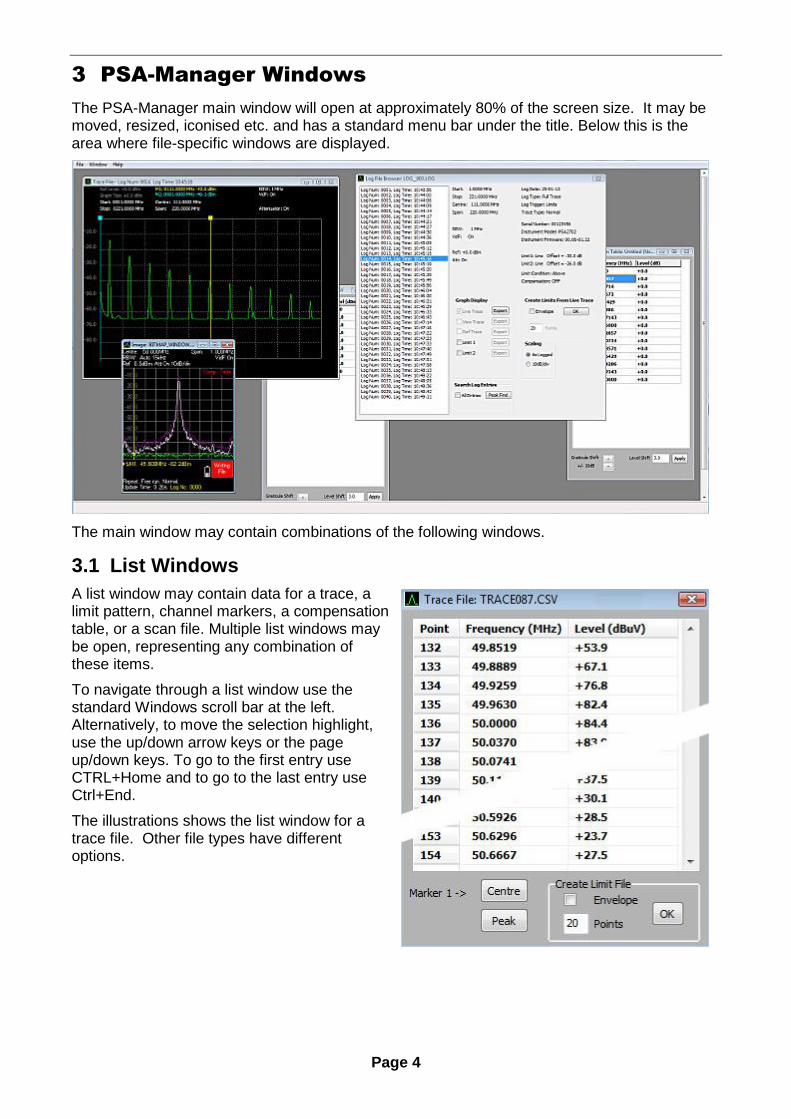
The PSA-Manager main window will open at approximately 80% of the screen size. It may be moved, resized, iconised etc. and has a standard menu bar under the title. Below this is the area where file-specific windows are displayed.

The main window may contain combinations of the following windows.

3.1 List Windows

A list window may contain data for a trace, a limit pattern, channel markers, a compensation table, or a scan file. Multiple list windows may be open, representing any combination of these items.

To navigate through a list window use the standard Windows scroll bar at the left. Alternatively, to move the selection highlight, use the up/down arrow keys or the page up/down keys. To go to the first entry use CTRL+Home and to go to the last entry use Ctrl+End.

The illustrations shows the list window for a trace file. Other file types have different options.

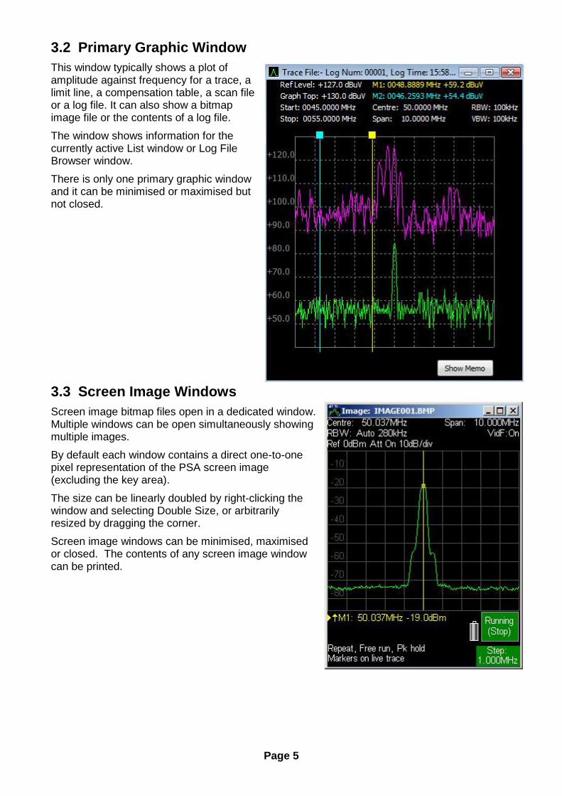
3.2 Primary Graphic Window

This window typically shows a plot of amplitude against frequency for a trace, a limit line, a compensation table, a scan file or a log file. It can also show a bitmap image file or the contents of a log file.

The window shows information for the currently active List window or Log File Browser window.

There is only one primary graphic window and it can be minimised or maximised but not closed.

3.3 Screen Image Windows

Screen image bitmap files open in a dedicated window. Multiple windows can be open simultaneously showing multiple images.

By default each window contains a direct one-to-one pixel representation of the PSA screen image (excluding the key area).

The size can be linearly doubled by right-clicking the window and selecting Double Size, or arbitrarily resized by dragging the corner.

Screen image windows can be minimised, maximised or closed. The contents of any screen image window can be printed.

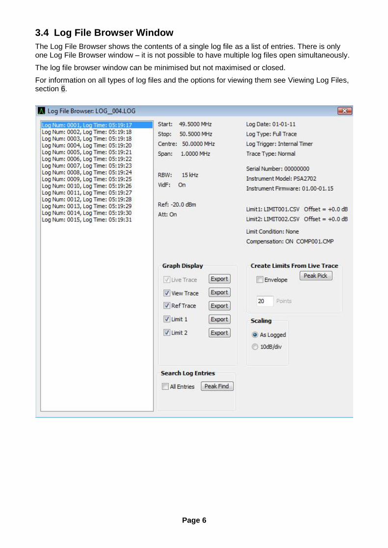
3.4 Log File Browser Window

The Log File Browser shows the contents of a single log file as a list of entries. There is only one Log File Browser window – it is not possible to have multiple log files open simultaneously.

The log file browser window can be minimised but not maximised or closed.

For information on all types of log files and the options for viewing them see Viewing Log Files, section 6.

4 Viewing Trace Files

Trace files stored on the PSA must be transferred from the PSA\TRACES folder to the TRACES folder on the PC which is a sub-folder of the Home folder (see section 2.1). This can be done either using a USB Flash drive or by direct USB connection and “Link to PC” (Setup/Functions > System/File Ops > File Ops > Link to PC).

Trace files have a .CSV extension and do NOT start with a $ symbol.

To view a trace file use File > Open > Trace File which will show the contents of the appropriate folder for traces.

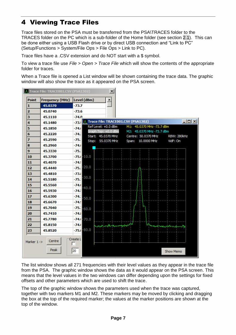
When a Trace file is opened a List window will be shown containing the trace data. The graphic window will also show the trace as it appeared on the PSA screen.

The list window shows all 271 frequencies with their level values as they appear in the trace file from the PSA. The graphic window shows the data as it would appear on the PSA screen. This means that the level values in the two windows can differ depending upon the settings for fixed offsets and other parameters which are used to shift the trace.

The top of the graphic window shows the parameters used when the trace was captured, together with two markers M1 and M2. These markers may be moved by clicking and dragging the box at the top of the required marker; the values at the marker positions are shown at the top of the window.

The list window selection highlight will track the position of M1 and moving the selection highlight in the list window will cause M1 to track in the graphic window. M1 may be moved to the centre frequency or highest peak by clicking the appropriate button at the bottom of the list window. It is not possible to edit the data in a trace file.

4.1.1 The Trace Memo sub-window

Operating the Show Memo button on the graphics window opens a Memo window into which explanatory notes can be typed. The memo contents are automatically saved as the they are typed and it is not necessary to re-save the file. The window can be closed with Hide Memo so that it does not obscure the bottom of the graticule area.

The memo contents are stored in a linked file with the extension .MEM. The original PSA trace file is not altered.

4.1.2 Printing Trace Files

The contents of the graphics window can be printed onto any connected printer or to a print file using File > Print. Ensure that the window "focus" is on the graphics window by clicking it before printing. The memo contents, if any, will also be printed below the graticule area.

4.1.3 Creating Limit Patterns from Trace Files

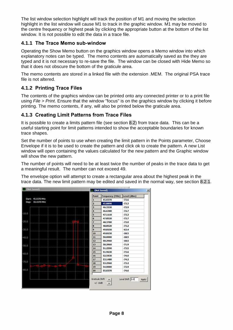
It is possible to create a limits pattern file (see section 8.2) from trace data. This can be a useful starting point for limit patterns intended to show the acceptable boundaries for known trace shapes.

Set the number of points to use when creating the limit pattern in the Points parameter, Choose Envelope if it is to be used to create the pattern and click ok to create the pattern. A new List window will open containing the values calculated for the new pattern and the Graphic window will show the new pattern.

The number of points will need to be at least twice the number of peaks in the trace data to get a meaningful result. The number can not exceed 49.

The envelope option will attempt to create a rectangular area about the highest peak in the trace data. The new limit pattern may be edited and saved in the normal way, see section 8.2.1.

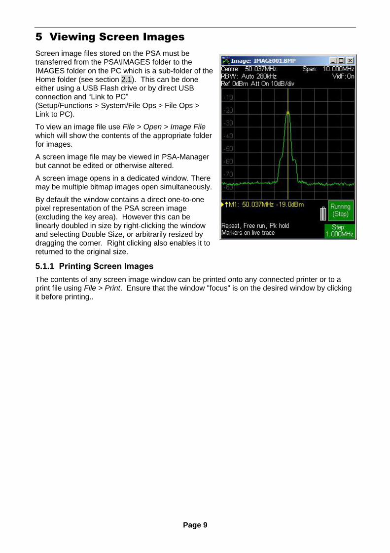
5 Viewing Screen Images

Screen image files stored on the PSA must be transferred from the PSA\IMAGES folder to the IMAGES folder on the PC which is a sub-folder of the Home folder (see section 2.1). This can be done either using a USB Flash drive or by direct USB connection and “Link to PC” (Setup/Functions > System/File Ops > File Ops > Link to PC).

To view an image file use File > Open > Image File which will show the contents of the appropriate folder for images.

A screen image file may be viewed in PSA-Manager but cannot be edited or otherwise altered.

A screen image opens in a dedicated window. There may be multiple bitmap images open simultaneously.

By default the window contains a direct one-to-one pixel representation of the PSA screen image (excluding the key area). However this can be linearly doubled in size by right-clicking the window and selecting Double Size, or arbitrarily resized by dragging the corner. Right clicking also enables it to returned to the original size.

5.1.1 Printing Screen Images

The contents of any screen image window can be printed onto any connected printer or to a print file using File > Print. Ensure that the window "focus" is on the desired window by clicking it before printing..

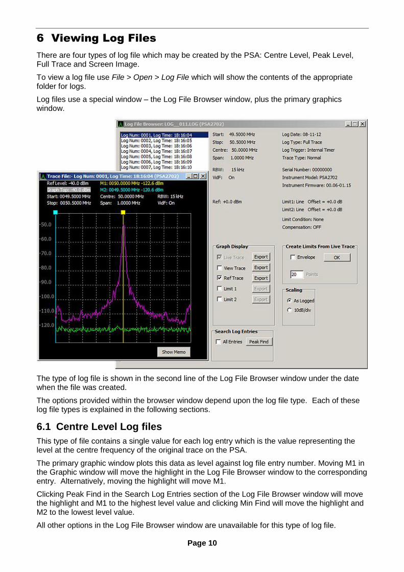
6 Viewing Log Files

There are four types of log file which may be created by the PSA: Centre Level, Peak Level, Full Trace and Screen Image.

To view a log file use File > Open > Log File which will show the contents of the appropriate folder for logs.

Log files use a special window – the Log File Browser window, plus the primary graphics window.

The type of log file is shown in the second line of the Log File Browser window under the date when the file was created.

The options provided within the browser window depend upon the log file type. Each of these log file types is explained in the following sections.

6.1 Centre Level Log files

This type of file contains a single value for each log entry which is the value representing the level at the centre frequency of the original trace on the PSA.

The primary graphic window plots this data as level against log file entry number. Moving M1 in the Graphic window will move the highlight in the Log File Browser window to the corresponding entry. Alternatively, moving the highlight will move M1.

Clicking Peak Find in the Search Log Entries section of the Log File Browser window will move the highlight and M1 to the highest level value and clicking Min Find will move the highlight and M2 to the lowest level value.

All other options in the Log File Browser window are unavailable for this type of log file.

6.2 Peak Level Log files

This file type contains two values for each log entry these being the level at the highest peak in the trace together with the corresponding frequency value.

Choose Peak Level or Peak Frequency in the Graph Display section of the Log File Browser window to see either level plotted against log file entry or frequency against log file entry.

Moving M1 in the Graphics window will move the highlight in the Log File Browser window to the corresponding entry. alternatively, moving the highlight will move M1.

Clicking Peak Find in the Search Log Entries section of the Log File Browser window will move the highlight and M1 to the highest level value and clicking Min Find will move the highlight and M2 to the lowest level value.

All other options in the Log File Browser window are unavailable for this type of log file.

6.3 Full Trace Log files

This file type contains the complete trace data for each log file entry. The Graphic window shows the trace for the entry at the highlight in the Log File Browser window.

If the log file was captured with the PSA scale and shift function selected the Scaling section of the Log File Browser may be used to reset the scaling to 10dB/div. The data, as captured, may be viewed by selecting As Logged.

The Live Trace is always shown and cannot be removed from the Graphic window. If the log file contains a View Trace or Ref Trace these may be shown in the Graphic window by checking the appropriate boxes in the Graph Display section of the Browser window. If the log file contains a limit pattern for Limit 1 or Limit 2 these may be shown in the same way. Items not available will be greyed out.

Use the Search Log Entries section of the Log File Browser window to find the highest peak. Clicking Find Peak with All Entries un-checked will look in the trace of the currently selected log file entry, with All Entries checked all traces in all log-file entries will be searched. When the search is complete the Graphic window will show the trace with marker M1 positioned at the peak.



There is only one memo field per log file which is applied to all entries.

The memo contents are stored in a linked file with the extension .MEM. The original PSA log file is not altered.

6.3.2 Exporting from Full Trace Log Files

Any of the traces or limit lines can be exported as a CSV file. Click the Export box in the Graph Display section of the Browser window to export the chosen item from the log file. A Windows file Save-As dialog will appear to allow the exported data to be written to a file.

6.3.3 Creating Limit Patterns from Trace Log Files

To create a new limits pattern file from the live trace data use the Create Limits From Live Trace section of the Browser window. Set the number of points to use when creating the limit pattern in the Points parameter, Choose Envelope if it is to be used to create the pattern and click OK to create the pattern. A new List window will open containing the values calculated for the new pattern and the Graphic window will show the new pattern.

The number of points will need to be at least twice the number of peaks in the trace data to get a meaningful result. The envelope option will attempt to create a rectangular area about the highest peak in the trace data. The new limit pattern may be edited and saved in the normal way, see section 8.2.1.

6.4 Screen Image Log files

This log file type contains a bitmap image of the trace for each log file entry. Moving the Highlight through the Log File Browser list will show the bitmap image at each entry.

Note that screen images within a log file are shown in the primary graphics window which opens at the size created by its last use. Right clicking the window enables the image to be scaled at its original size within the PSA, or double that size.

6.4.1 Exporting from Screen Image Log Files

To export the entry to a Windows bitmap image file select Export in the Screen Image Log section of the Log File Browser window. A Windows file Save-As dialog will appear to allow the exported data to be written to a file.

6.5 Printing from Log Files

The contents of the primary graphics window for any log file type can be printed onto any connected printer or to a print file using File > Print. Ensure that the window "focus" is on the graphics window by clicking it before printing.

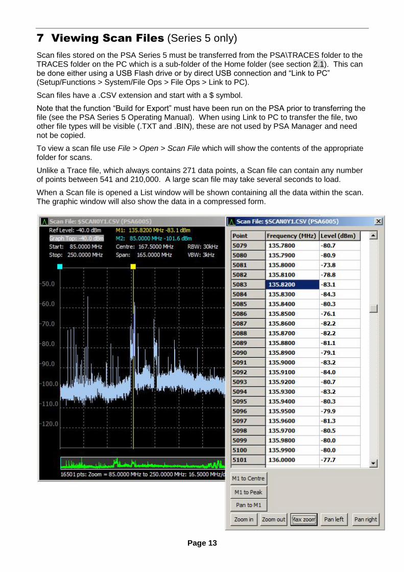
7 Viewing Scan Files (Series 5 only)

Scan files stored on the PSA Series 5 must be transferred from the PSA\TRACES folder to the TRACES folder on the PC which is a sub-folder of the Home folder (see section 2.1). This can be done either using a USB Flash drive or by direct USB connection and “Link to PC” (Setup/Functions > System/File Ops > File Ops > Link to PC).

Scan files have a .CSV extension and start with a $ symbol.

Note that the function “Build for Export” must have been run on the PSA prior to transferring the file (see the PSA Series 5 Operating Manual). When using Link to PC to transfer the file, two other file types will be visible (.TXT and .BIN), these are not used by PSA Manager and need not be copied.

To view a scan file use File > Open > Scan File which will show the contents of the appropriate folder for scans.

Unlike a Trace file, which always contains 271 data points, a Scan file can contain any number of points between 541 and 210,000. A large scan file may take several seconds to load.

When a Scan file is opened a List window will be shown containing all the data within the scan. The graphic window will also show the data in a compressed form.

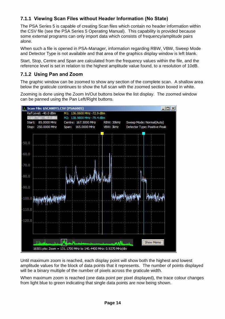
7.1.1 Viewing Scan Files without Header Information (No State)

The PSA Series 5 is capable of creating Scan files which contain no header information within the CSV file (see the PSA Series 5 Operating Manual). This capability is provided because some external programs can only import data which consists of frequency/amplitude pairs alone.

When such a file is opened in PSA-Manager, information regarding RBW, VBW, Sweep Mode and Detector Type is not available and that area of the graphics display window is left blank.

Start, Stop, Centre and Span are calculated from the frequency values within the file, and the reference level is set in relation to the highest amplitude value found, to a resolution of 10dB.

7.1.2 Using Pan and Zoom

The graphic window can be zoomed to show any section of the complete scan. A shallow area below the graticule continues to show the full scan with the zoomed section boxed in white.

Zooming is done using the Zoom In/Out buttons below the list display. The zoomed window can be panned using the Pan Left/Right buttons.

Until maximum zoom is reached, each display point will show both the highest and lowest amplitude values for the block of data points that it represents. The number of points displayed will be a binary multiple of the number of pixels across the graticule width.

When maximum zoom is reached (one data point per pixel displayed), the trace colour changes from light blue to green indicating that single data points are now being shown.

The List display shows the twenty data values around the M1 marker position. Depending upon the zoom level, each displayed point can represent a block of list values. The M1 marker position can be changed either by grabbing its handle (the coloured square at the top) and dragging, or by using the keyboard controls Arrow-Up/Down and Page Up/Down.

The M2 marker position (blue) can only be changed by dragging its handle.

Moving the M1 marker with keyboard controls allows it to be moved outside of the zoomed window and anywhere within the full scan.

The button Pan to M1 can then be used to reposition the zoomed window.

M1 to Centre and M1 to Peak reposition the marker based upon the full scan data and not just the data within the zoomed window.

The Max Zoom button changes function to become Show All (display the full scan) once maximum zoom has been reached.



The memo contents are stored in a linked file with the extension .MEM. The original PSA scan file is not altered.

7.1.4 Printing from Scan Files

The contents of the graphics window can be printed onto any connected printer or to a print file using File > Print. Ensure that the window "focus" is on the graphics window by clicking it before printing. The memo contents, if any, will also be printed below the graticule area.

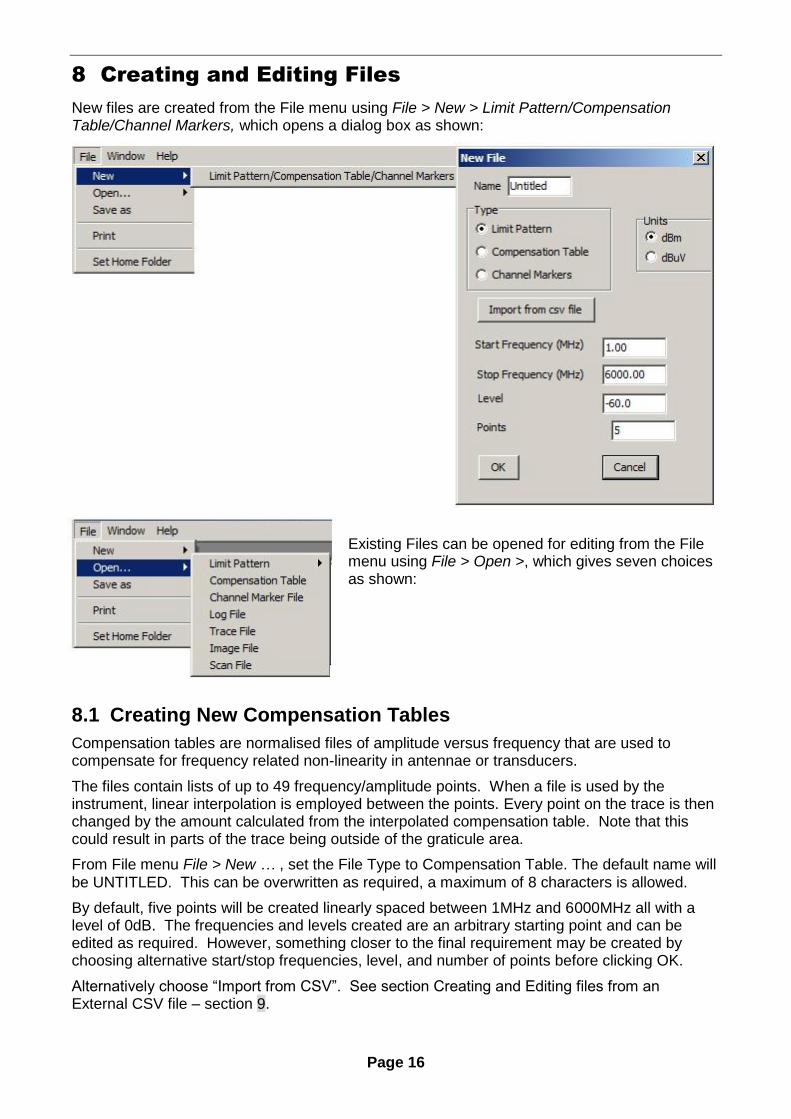
8 Creating and Editing Files

New files are created from the File menu using File > New > Limit Pattern/Compensation Table/Channel Markers, which opens a dialog box as shown:

Existing Files can be opened for editing from the File menu using File > Open >, which gives seven choices as shown:

8.1 Creating New Compensation Tables

Compensation tables are normalised files of amplitude versus frequency that are used to compensate for frequency related non-linearity in antennae or transducers.

The files contain lists of up to 49 frequency/amplitude points. When a file is used by the instrument, linear interpolation is employed between the points. Every point on the trace is then changed by the amount calculated from the interpolated compensation table. Note that this could result in parts of the trace being outside of the graticule area.

From File menu File > New … , set the File Type to Compensation Table. The default name will be UNTITLED. This can be overwritten as required, a maximum of 8 characters is allowed.

By default, five points will be created linearly spaced between 1MHz and 6000MHz all with a level of 0dB. The frequencies and levels created are an arbitrary starting point and can be edited as required. However, something closer to the final requirement may be created by choosing alternative start/stop frequencies, level, and number of points before clicking OK.

Alternatively choose “Import from CSV”. See section Creating and Editing files from an External CSV file – section 9.

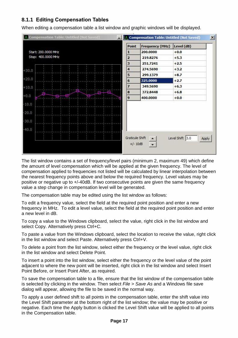
8.1.1 Editing Compensation Tables

When editing a compensation table a list window and graphic windows will be displayed.

The list window contains a set of frequency/level pairs (minimum 2, maximum 49) which define the amount of level compensation which will be applied at the given frequency. The level of compensation applied to frequencies not listed will be calculated by linear interpolation between the nearest frequency points above and below the required frequency. Level values may be positive or negative up to +/-40dB. If two consecutive points are given the same frequency value a step change in compensation level will be generated.

The compensation table may be edited using the list window as follows:

To edit a frequency value, select the field at the required point position and enter a new frequency in MHz. To edit a level value, select the field at the required point position and enter a new level in dB.

To copy a value to the Windows clipboard, select the value, right click in the list window and select Copy. Alternatively press Ctrl+C.

To paste a value from the Windows clipboard, select the location to receive the value, right click in the list window and select Paste. Alternatively press Ctrl+V.

To delete a point from the list window, select either the frequency or the level value, right click in the list window and select Delete Point.

To insert a point into the list window, select either the frequency or the level value of the point adjacent to where the new point will be inserted, right click in the list window and select Insert Point Before, or Insert Point After, as required.

To save the compensation table to a file, ensure that the list window of the compensation table is selected by clicking in the window. Then select File > Save As and a Windows file save dialog will appear, allowing the file to be saved in the normal way.

To apply a user defined shift to all points in the compensation table, enter the shift value into the Level Shift parameter at the bottom right of the list window; the value may be positive or negative. Each time the Apply button is clicked the Level Shift value will be applied to all points in the Compensation table.

To move the view in the graphic window, to see points that are off the top or bottom of the graph, click the up and down arrow keys of the Graticule Shift parameter at the bottom left of the list window ; the graph view is moved up or down in 10dB steps. The Graticule Shift parameter does not change the level values in the compensation table.

The compensation table may be edited using the graphic window as follows:

To edit the frequency and level value of a point, click the point and drag to the required position. Note: whenever a point is clicked in the graphic window that point will automatically be highlighted in the list window.

To edit the frequency value of a point, hold down the control key then click and drag the required point to the new frequency.

To edit the level value of a point, hold down the shift key then click and drag the required point to the new level.

To delete a point from the graphic window, right click on the required point and select Delete Point.

To insert a point into the graphic window, right click on the required point and select either Insert Point Before, or Insert Point After, as required.

8.1.2 Transferring and Using Compensation Tables

Compensation Table files created under PSA-Manager are stored in the TABLES folder (by default this will be My Documents\PSAman\TABLES). Compensation Tables are identified by having the extension .CMP. (N.B. the PC must be set to show file extensions – see section 2.)

These must be transferred to the TABLES folder of the instrument (PSA\TABLES) using either a USB Flash drive or direct USB connection and “Link to PC” (Setup/Functions > System/File Ops > File Ops > Link to PC)

A Compensation Table is loaded from the Level/Limits menu using: Level/Limits > Offset/Tables > Set > Comp. Table > Select Table This opens the file browser window to show the tables currently available. Once loaded the file name appears within the Compensation Table sub-menu screen, and it can be turned Off or back On without the need to re-load the file.

8.2 Creating New Limit Patterns

Limit Patterns can be displayed on the screen of the PSA They can have multiple levels and can include vertical steps and angled lines. Patterns are contained within files that are lists of up to 49 frequency/amplitude points. When a file is used by the instrument, linear interpolation is employed between the points. Up to two patterns can be displayed simultaneously in different colours (red and blue).

Lines or patterns may be used as simple visual aids to determine whether a signal is within a specific level range, or they may be used in conjunction with the Limits Comparator to create an automatic action.

From File menu File > New … set the File Type to Limit Pattern. The default name will be UNTITLED. This can be overwritten as required, a maximum of 8 characters is allowed. Choose the Units as dBm or dBuV as required.

By default, five points will be created linearly spaced between 1MHz and 6000MHz all with a level of -60dBm (or +47dBuV). The frequencies and levels created are an arbitrary starting point and can be edited as required. However, something closer to the final requirement may be created by choosing alternative start/stop frequencies, level, and number of points before clicking OK.


A further facility is provided to use an existing Trace file as the basis for a limit pattern – see section 4.1.3.

8.2.1 Editing Limit Patterns

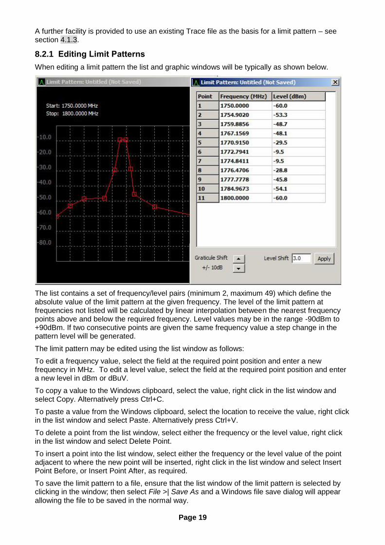
When editing a limit pattern the list and graphic windows will be typically as shown below.

The list contains a set of frequency/level pairs (minimum 2, maximum 49) which define the absolute value of the limit pattern at the given frequency. The level of the limit pattern at frequencies not listed will be calculated by linear interpolation between the nearest frequency points above and below the required frequency. Level values may be in the range -90dBm to +90dBm. If two consecutive points are given the same frequency value a step change in the pattern level will be generated.

The limit pattern may be edited using the list window as follows:

To edit a frequency value, select the field at the required point position and enter a new frequency in MHz. To edit a level value, select the field at the required point position and enter a new level in dBm or dBuV.

To copy a value to the Windows clipboard, select the value, right click in the list window and select Copy. Alternatively press Ctrl+C.

To paste a value from the Windows clipboard, select the location to receive the value, right click in the list window and select Paste. Alternatively press Ctrl+V.

To delete a point from the list window, select either the frequency or the level value, right click in the list window and select Delete Point.

To insert a point into the list window, select either the frequency or the level value of the point adjacent to where the new point will be inserted, right click in the list window and select Insert Point Before, or Insert Point After, as required.

To save the limit pattern to a file, ensure that the list window of the limit pattern is selected by clicking in the window; then select File >| Save As and a Windows file save dialog will appear allowing the file to be saved in the normal way.

To apply a user defined shift to all points in the limit pattern, enter the shift value into the Level Shift parameter at the bottom right of the list window; the value may be positive or negative. Each time the Apply button is clicked the Level Shift value will be applied to all points in the limit pattern.

To move the view in the graphic window, to see points that are off the top or bottom of the graph, click the up and down arrow keys of the Graticule Shift parameter at the bottom left of the list window; the graph view moves up or down in 10dB steps. The Graticule Shift parameter does not change the level values in the limit pattern.

The limit pattern may be edited using the graphic window as follows:

To edit the frequency and level value of a point, click the point and drag to the required position. Note: whenever a point is clicked in the graphic window that point will automatically be highlighted in the list window.

To edit the frequency value of a point, hold down the control key then click and drag the required point to the new frequency. To edit the level value of a point, hold down the shift key then click and drag the required point to the new level.

To delete a point from the graphic window, right click on the required point and select Delete Point.

To insert a point into the graphic window, right click on the required point and select either Insert Point Before, or Insert Point After, as required.

8.2.2 Transferring and Using Limit Patterns

Limit Pattern files created under PSA-Manager are stored in the TABLES folder (by default this will be My Documents\PSAman\TABLES). Limit Patterns are identified by having the extension .CSV and having file names that do not begin with $. (N.B. the PC must be set to show file extensions – see section 2.)

These must be transferred to the TABLES folder of the instrument (PSA\TABLES) using either a USB Flash drive or direct USB connection and “Link to PC” (Setup/Functions > System/File Ops > File Ops > Link to PC)

A Limit Pattern is loaded from the Level/Limits menu using: Level/Limits > Limits > Set Limits > (Limit 1/Limit 2) > Select Pattern This opens the file browser window to show the limit patterns and channel markers currently available. Choose a limit pattern (file names not starting with a $ symbol). Once loaded the file name appears within the Limits sub-menu screen, and it can be turned Off or back On without the need to re-load the file.

8.3 Creating New Channel Markers

Channel Markers are a special case of a Limit Pattern which consists only of vertical lines at frequency points defined within the file. These can be displayed as an alternative to limit lines/patterns on the PSA. Up to two files can be displayed simultaneously in differing colours. Each file can contain up to 49 frequency points.

From File menu File > New … set the File Type to Channel Markers. The default name will be $UNTITLE. This can be overwritten as required, a maximum of 8 characters is allowed including the $ with which the name must always commence.

By default, five points will be created linearly spaced between 1MHz and 6000MHz. Choosing different start/stop frequencies and numbers of points will enable equally spaced channel frequencies to be created which may require no further editing.


Unlike Limit Patterns which require a minimum of two points, a channel markers file can contain only a single point.

8.3.1 Editing Channel Markers

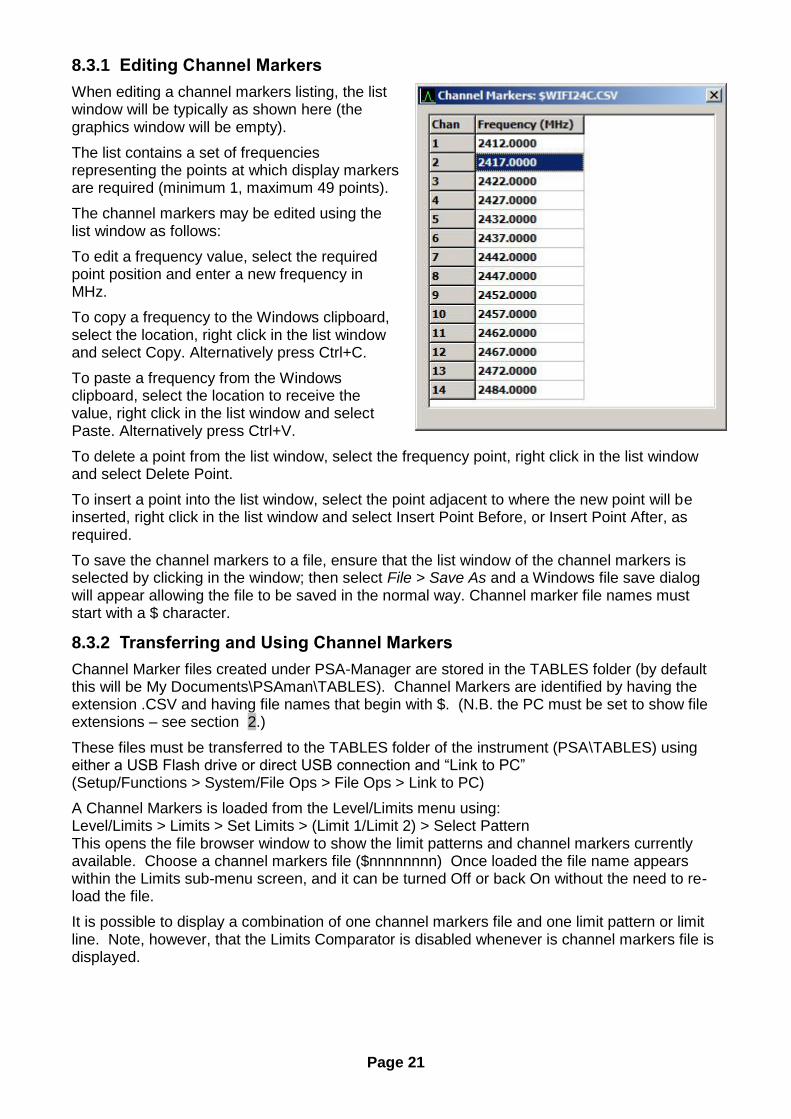
When editing a channel markers listing, the list window will be typically as shown here (the graphics window will be empty).

The list contains a set of frequencies representing the points at which display markers are required (minimum 1, maximum 49 points).

The channel markers may be edited using the list window as follows:

To edit a frequency value, select the required point position and enter a new frequency in MHz.

To copy a frequency to the Windows clipboard, select the location, right click in the list window and select Copy. Alternatively press Ctrl+C.

To paste a frequency from the Windows clipboard, select the location to receive the value, right click in the list window and select Paste. Alternatively press Ctrl+V.

To delete a point from the list window, select the frequency point, right click in the list window and select Delete Point.

To insert a point into the list window, select the point adjacent to where the new point will be inserted, right click in the list window and select Insert Point Before, or Insert Point After, as required.

To save the channel markers to a file, ensure that the list window of the channel markers is selected by clicking in the window; then select File > Save As and a Windows file save dialog will appear allowing the file to be saved in the normal way. Channel marker file names must start with a $ character.

8.3.2 Transferring and Using Channel Markers

Channel Marker files created under PSA-Manager are stored in the TABLES folder (by default this will be My Documents\PSAman\TABLES). Channel Markers are identified by having the extension .CSV and having file names that begin with $. (N.B. the PC must be set to show file extensions – see section 2.)

These files must be transferred to the TABLES folder of the instrument (PSA\TABLES) using either a USB Flash drive or direct USB connection and “Link to PC” (Setup/Functions > System/File Ops > File Ops > Link to PC)

A Channel Markers is loaded from the Level/Limits menu using: Level/Limits > Limits > Set Limits > (Limit 1/Limit 2) > Select Pattern This opens the file browser window to show the limit patterns and channel markers currently available. Choose a channel markers file ($nnnnnnnn) Once loaded the file name appears within the Limits sub-menu screen, and it can be turned Off or back On without the need to re-load the file.

It is possible to display a combination of one channel markers file and one limit pattern or limit line. Note, however, that the Limits Comparator is disabled whenever is channel markers file is displayed.

9 Importing Data from External CSV Files

As an alternative to manual creation, Limit Patterns, Channel Marker Lists and Compensation Tables can be created by importing an external .CSV (comma separated variable) file.

Upon choosing “Import from CSV” from the File > New dialog box, a file browsing window will open from which the required file can be selected. By default the initial folder will be one called IMPORTS which is a sub-folder of the Home folder (see section 2.1).

To be successfully loaded, the file must conform to a number of rules:

1. No header line must exist (i.e. the first line must contain frequency or frequency/amplitude data)

2. The first column must contain the numeric frequency point values in MHz within the range 1MHz to 6000MHz.

3. The frequency point value in each line must be equal to or higher than that of the previous line for Limit Patterns and Compensation Tables, and higher than that of the previous line for Channel Marker Lists.

4. For Limit Patterns and Compensation Tables only the second column must contain numeric values in dB (or dBm depending upon application) between -120 and +120.

5. The maximum number of characters within one line must not exceed 100.

6. Each line including the last line must contain a new-line character (LF or LF/CR).

If the file does not conform with these rules it will be rejected and an error message will be displayed. The following points should also be noted:

Only the first 49 lines will be imported.

…Numbers can contain any number of digits of resolution but will be truncated on import to 4 decimal places for frequencies and one decimal place for amplitudes.

Letters following the numeric values (e.g. 1845.00MHz or -2.35dBm) are allowable and will be ignored.

Columns to the right of the frequency/amplitude columns are allowable and will be ignored (subject to the 100 characters per line limit).

Where the user is starting with an existing CSV file, as might be supplied with an antenna or transducer, the file should be examined within a editor such as Excel and modified so as to conform to the above rules. This may involve deleting any header lines, deleting or re-ordering columns, and applying a simple mathematic operation to ensure that the units are correct (e.g. convert kHz to MHz). The file must then be re-saved as a CSV (comma delimited) file type.

It is also possible to create a valid file using a simple text editor such as Notepad. For Channel Marker Lists each frequency should be placed on a new line ensuring that a new empty line is created at the end. For Limit Patterns and Compensation Tables each frequency should be followed by a comma followed by the corresponding amplitude with each pair placed on a new line, and ensuring that a new empty line is created at the end. The file can be saved with a .csv extension or with a .txt extension, in the latter case the file browser dialog box will need to be set to All File types.

____________________________________________________________________________

Aim-TTi PSA-Manager version 3 User Guide Issue – May 2015

PSA-Manager Version 3 User Manual -...

Documents

Transcript of PSA-Manager Version 3 User Manual -...