Prototypage Rapide et Génération de Code pour DSP Multi ...
211
HAL Id: tel-00578043 https://tel.archives-ouvertes.fr/tel-00578043 Submitted on 18 Mar 2011 HAL is a multi-disciplinary open access archive for the deposit and dissemination of sci- entific research documents, whether they are pub- lished or not. The documents may come from teaching and research institutions in France or abroad, or from public or private research centers. L’archive ouverte pluridisciplinaire HAL, est destinée au dépôt et à la diffusion de documents scientifiques de niveau recherche, publiés ou non, émanant des établissements d’enseignement et de recherche français ou étrangers, des laboratoires publics ou privés. Prototypage Rapide et Génération de Code pour DSP Multi-Coeurs Appliqués à la Couche Physique des Stations de Base 3GPP LTE Maxime Pelcat To cite this version: Maxime Pelcat. Prototypage Rapide et Génération de Code pour DSP Multi-Coeurs Appliqués à la Couche Physique des Stations de Base 3GPP LTE. Réseaux et télécommunications [cs.NI]. INSA de Rennes, 2010. Français. NNT : 2010ISAR0011. tel-00578043
Transcript of Prototypage Rapide et Génération de Code pour DSP Multi ...
HAL Id: tel-00578043https://tel.archives-ouvertes.fr/tel-00578043
Submitted on 18 Mar 2011
HAL is a multi-disciplinary open accessarchive for the deposit and dissemination of sci-entific research documents, whether they are pub-lished or not. The documents may come fromteaching and research institutions in France orabroad, or from public or private research centers.
L’archive ouverte pluridisciplinaire HAL, estdestinée au dépôt et à la diffusion de documentsscientifiques de niveau recherche, publiés ou non,émanant des établissements d’enseignement et derecherche français ou étrangers, des laboratoirespublics ou privés.
Prototypage Rapide et Génération de Code pour DSPMulti-Coeurs Appliqués à la Couche Physique des
Stations de Base 3GPP LTEMaxime Pelcat
To cite this version:Maxime Pelcat. Prototypage Rapide et Génération de Code pour DSP Multi-Coeurs Appliqués à laCouche Physique des Stations de Base 3GPP LTE. Réseaux et télécommunications [cs.NI]. INSA deRennes, 2010. Français. �NNT : 2010ISAR0011�. �tel-00578043�

Thèse
THESE INSA Rennessous le sceau de l’Université européenne de Bretagne
pour obtenir le titre deDOCTEUR DE L’INSA DE RENNES
Spécialité : Traitement du Signal et des Images
présentée par
Maxime PelcatECOLE DOCTORALE : MATISSELABORATOIRE : IETR
Rapid Prototyping and Dataflow-Based
Code Generation for the 3GPP LTE
eNodeB Physical Layer Mapped onto
Multi-Core DSPs
Thèse soutenue le 17.09.2010devant le jury composé de :Shuvra BHATTACHARYYAProfesseur à l’Université du Maryland (USA) / PrésidentGuy GOGNIATProfesseur des Universités à l’Université de Bretagne Sud / RapporteurChristophe JEGOProfesseur des Universités à l’Institut Polytechnique de Bordeaux / RapporteurSébastien LE NOURSMaître de conférences à Polytech’ Nantes / ExaminateurSlaheddine ARIDHIDocteur / EncadrantJean-François NEZANProfesseur des universités à l’INSA de Rennes / Directeur de thèse

Contents
Acknowledgements 1
1 Introduction 3
1.1 Overview . . . . . . . . . . . . . . . . . . . . . . . . . . . . . . . . . . . . . 3
1.2 Contributions of this Thesis . . . . . . . . . . . . . . . . . . . . . . . . . . . 7
1.3 Outline of this Thesis . . . . . . . . . . . . . . . . . . . . . . . . . . . . . . 7
I Background 9
2 3GPP Long Term Evolution 11
2.1 Introduction . . . . . . . . . . . . . . . . . . . . . . . . . . . . . . . . . . . . 11
2.1.1 Evolution and Environment of 3GPP Telecommunication Systems . 11
2.1.2 Terminology and Requirements of LTE . . . . . . . . . . . . . . . . . 12
2.1.3 Scope and Organization of the LTE Study . . . . . . . . . . . . . . . 14
2.2 From IP Packets to Air Transmission . . . . . . . . . . . . . . . . . . . . . . 15
2.2.1 Network Architecture . . . . . . . . . . . . . . . . . . . . . . . . . . 15
2.2.2 LTE Radio Link Protocol Layers . . . . . . . . . . . . . . . . . . . . 16
2.2.3 Data Blocks Segmentation and Concatenation . . . . . . . . . . . . . 17
2.2.4 MAC Layer Scheduler . . . . . . . . . . . . . . . . . . . . . . . . . . 18
2.3 Overview of LTE Physical Layer Technologies . . . . . . . . . . . . . . . . . 18
2.3.1 Signal Air transmission and LTE . . . . . . . . . . . . . . . . . . . . 18
2.3.2 Selective Channel Equalization . . . . . . . . . . . . . . . . . . . . . 20
2.3.3 eNodeB Physical Layer Data Processing . . . . . . . . . . . . . . . . 21
2.3.4 Multicarrier Broadband Technologies and Resources . . . . . . . . . 22
2.3.5 LTE Modulation and Coding Scheme . . . . . . . . . . . . . . . . . 26
2.3.6 Multiple Antennas . . . . . . . . . . . . . . . . . . . . . . . . . . . . 29
2.4 LTE Uplink Features . . . . . . . . . . . . . . . . . . . . . . . . . . . . . . . 30
2.4.1 Single Carrier-Frequency Division Multiplexing . . . . . . . . . . . . 30
2.4.2 Uplink Physical Channels . . . . . . . . . . . . . . . . . . . . . . . . 31
2.4.3 Uplink Reference Signals . . . . . . . . . . . . . . . . . . . . . . . . . 33
2.4.4 Uplink Multiple Antenna Techniques . . . . . . . . . . . . . . . . . . 34
2.4.5 Random Access Procedure . . . . . . . . . . . . . . . . . . . . . . . . 35
2.5 LTE Downlink Features . . . . . . . . . . . . . . . . . . . . . . . . . . . . . 37
i

ii CONTENTS
2.5.1 Orthogonal Frequency Division Multiplexing Access . . . . . . . . . 37
2.5.2 Downlink Physical Channels . . . . . . . . . . . . . . . . . . . . . . 38
2.5.3 Downlink Reference Signals . . . . . . . . . . . . . . . . . . . . . . . 40
2.5.4 Downlink Multiple Antenna Techniques . . . . . . . . . . . . . . . . 40
2.5.5 UE Synchronization . . . . . . . . . . . . . . . . . . . . . . . . . . . 42
3 Dataflow Model of Computation 45
3.1 Introduction . . . . . . . . . . . . . . . . . . . . . . . . . . . . . . . . . . . . 45
3.1.1 Model of Computation Overview . . . . . . . . . . . . . . . . . . . . 45
3.1.2 Dataflow Model of Computation Overview . . . . . . . . . . . . . . . 47
3.2 Synchronous Data Flow . . . . . . . . . . . . . . . . . . . . . . . . . . . . . 50
3.2.1 SDF Schedulability . . . . . . . . . . . . . . . . . . . . . . . . . . . . 50
3.2.2 Single Rate SDF . . . . . . . . . . . . . . . . . . . . . . . . . . . . . 52
3.2.3 Conversion to a Directed Acyclic Graph . . . . . . . . . . . . . . . . 53
3.3 Cyclo Static Data Flow . . . . . . . . . . . . . . . . . . . . . . . . . . . . . 53
3.3.1 CSDF Schedulability . . . . . . . . . . . . . . . . . . . . . . . . . . . 54
3.4 Dataflow Hierarchical Extensions . . . . . . . . . . . . . . . . . . . . . . . . 54
3.4.1 Parameterized Dataflow Modeling . . . . . . . . . . . . . . . . . . . 55
3.4.2 Interface-Based Hierarchical Dataflow . . . . . . . . . . . . . . . . . 57
4 Rapid Prototyping and Programming Multi-core Architectures 61
4.1 Introduction . . . . . . . . . . . . . . . . . . . . . . . . . . . . . . . . . . . . 61
4.1.1 The Middle-Grain Parallelism Level . . . . . . . . . . . . . . . . . . 61
4.2 Modeling Multi-Core Heterogeneous Architectures . . . . . . . . . . . . . . 63
4.2.1 Understanding Multi-Core Heterogeneous Real-Time Embedded DSPMPSoC . . . . . . . . . . . . . . . . . . . . . . . . . . . . . . . . . . 63
4.2.2 Literature on Architecture Modeling . . . . . . . . . . . . . . . . . . 64
4.3 Multi-core Programming . . . . . . . . . . . . . . . . . . . . . . . . . . . . . 65
4.3.1 Middle-Grain Parallelization Techniques . . . . . . . . . . . . . . . . 65
4.3.2 PREESM Among Multi-core Programming Tools . . . . . . . . . . . 67
4.4 Multi-core Scheduling . . . . . . . . . . . . . . . . . . . . . . . . . . . . . . 68
4.4.1 Multi-core Scheduling Strategies . . . . . . . . . . . . . . . . . . . . 68
4.4.2 Scheduling an Application under Constraints . . . . . . . . . . . . . 69
4.4.3 Existing Work on Scheduling Heuristics . . . . . . . . . . . . . . . . 70
4.5 Generating Multi-core Executable Code . . . . . . . . . . . . . . . . . . . . 73
4.5.1 Static Multi-core Code Execution . . . . . . . . . . . . . . . . . . . . 73
4.5.2 Managing Application Variations . . . . . . . . . . . . . . . . . . . . 74
4.6 Conclusion of the Background Part . . . . . . . . . . . . . . . . . . . . . . . 74
II Contributions 77
5 A System-Level Architecture Model 79
5.1 Introduction . . . . . . . . . . . . . . . . . . . . . . . . . . . . . . . . . . . . 79
5.1.1 Target Architectures . . . . . . . . . . . . . . . . . . . . . . . . . . . 79
5.1.2 Building a New Architecture Model . . . . . . . . . . . . . . . . . . 82
5.2 The System-Level Architecture Model . . . . . . . . . . . . . . . . . . . . . 83
5.2.1 The S-LAM operators . . . . . . . . . . . . . . . . . . . . . . . . . . 83
5.2.2 Connecting operators in S-LAM . . . . . . . . . . . . . . . . . . . . 83
5.2.3 Examples of S-LAM Descriptions . . . . . . . . . . . . . . . . . . . . 84

CONTENTS iii
5.2.4 The route model . . . . . . . . . . . . . . . . . . . . . . . . . . . . . 86
5.3 Transforming the S-LAM model into the route model . . . . . . . . . . . . . 88
5.3.1 Overview of the transformation . . . . . . . . . . . . . . . . . . . . . 88
5.3.2 Generating a route step . . . . . . . . . . . . . . . . . . . . . . . . . 88
5.3.3 Generating direct routes from the graph model . . . . . . . . . . . . 88
5.3.4 Generating the complete routing table . . . . . . . . . . . . . . . . . 89
5.4 Simulating a deployment using the route model . . . . . . . . . . . . . . . . 90
5.4.1 The message passing route step simulation with contention nodes . . 90
5.4.2 The message passing route step simulation without contention nodes 91
5.4.3 The DMA route step simulation . . . . . . . . . . . . . . . . . . . . 91
5.4.4 The shared memory route step simulation . . . . . . . . . . . . . . . 91
5.5 Role of S-LAM in the Rapid Prototyping Process . . . . . . . . . . . . . . . 92
5.5.1 Storing an S-LAM Graph . . . . . . . . . . . . . . . . . . . . . . . . 92
5.5.2 Hierarchical S-LAM Descriptions . . . . . . . . . . . . . . . . . . . . 92
6 Enhanced Rapid Prototyping 95
6.1 Introduction . . . . . . . . . . . . . . . . . . . . . . . . . . . . . . . . . . . . 95
6.1.1 The Multi-Core DSP Programming Constraints . . . . . . . . . . . . 95
6.1.2 Objectives of a Multi-Core Scheduler . . . . . . . . . . . . . . . . . . 96
6.2 A Flexible Rapid Prototyping Process . . . . . . . . . . . . . . . . . . . . . 97
6.2.1 Algorithm Transformations while Rapid Prototyping . . . . . . . . . 97
6.2.2 Scenarios: Separating Algorithm and Architecture . . . . . . . . . . 99
6.2.3 Workflows: Flows of Model Transformations . . . . . . . . . . . . . . 101
6.3 The Structure of the Scalable Multi-Core Scheduler . . . . . . . . . . . . . . 103
6.3.1 The Problem of Scheduling a DAG on an S-LAM Architecture . . . 104
6.3.2 Separating Heuristics from Benchmarks . . . . . . . . . . . . . . . . 104
6.3.3 Proposed ABC Sub-Modules . . . . . . . . . . . . . . . . . . . . . . 106
6.3.4 Proposed Actor Assignment Heuristics . . . . . . . . . . . . . . . . . 107
6.4 Advanced Features in Architecture Benchmark Computers . . . . . . . . . . 108
6.4.1 The route model in the AAM process . . . . . . . . . . . . . . . . . 108
6.4.2 The Infinite Homogeneous ABC . . . . . . . . . . . . . . . . . . . . 108
6.4.3 Minimizing Latency and Balancing Loads . . . . . . . . . . . . . . . 109
6.5 Scheduling Heuristics in the Framework . . . . . . . . . . . . . . . . . . . . 111
6.5.1 Assignment Heuristics . . . . . . . . . . . . . . . . . . . . . . . . . . 112
6.5.2 Ordering Heuristics . . . . . . . . . . . . . . . . . . . . . . . . . . . . 113
6.6 Quality Assessment of a Multi-Core Schedule . . . . . . . . . . . . . . . . . 114
6.6.1 Limits in Algorithm Middle-Grain Parallelism . . . . . . . . . . . . . 114
6.6.2 Upper Bound of the Algorithm Speedup . . . . . . . . . . . . . . . . 116
6.6.3 Lowest Acceptable Speedup Evaluation . . . . . . . . . . . . . . . . 116
6.6.4 Applying Scheduling Quality Assessment to Heterogeneous TargetArchitectures . . . . . . . . . . . . . . . . . . . . . . . . . . . . . . . 117
7 Dataflow LTE Models 119
7.1 Introduction . . . . . . . . . . . . . . . . . . . . . . . . . . . . . . . . . . . . 119
7.1.1 Elements of the Rapid Prototyping Framework . . . . . . . . . . . . 119
7.1.2 SDF4J : A Java Library for Algorithm Graph Transformations . . . 119
7.1.3 Graphiti : A Generic Graph Editor for Editing Architectures, Algo-rithms and Workflows . . . . . . . . . . . . . . . . . . . . . . . . . . 120

iv CONTENTS
7.1.4 PREESM : A Complete Framework for Hardware and Software Code-sign . . . . . . . . . . . . . . . . . . . . . . . . . . . . . . . . . . . . 121
7.2 Proposed LTE Models . . . . . . . . . . . . . . . . . . . . . . . . . . . . . . 121
7.2.1 Fixed and Variable eNodeB Parameters . . . . . . . . . . . . . . . . 121
7.2.2 A LTE eNodeB Use Case . . . . . . . . . . . . . . . . . . . . . . . . 122
7.2.3 The Different Parts of the LTE Physical Layer Model . . . . . . . . 124
7.3 Prototyping RACH Preamble Detection . . . . . . . . . . . . . . . . . . . . 124
7.4 Downlink Prototyping Model . . . . . . . . . . . . . . . . . . . . . . . . . . 128
7.5 Uplink Prototyping Model . . . . . . . . . . . . . . . . . . . . . . . . . . . . 129
7.5.1 PUCCH Decoding . . . . . . . . . . . . . . . . . . . . . . . . . . . . 130
7.5.2 PUSCH Decoding . . . . . . . . . . . . . . . . . . . . . . . . . . . . 131
8 Generating Code from LTE Models 135
8.1 Introduction . . . . . . . . . . . . . . . . . . . . . . . . . . . . . . . . . . . . 135
8.1.1 Execution Schemes . . . . . . . . . . . . . . . . . . . . . . . . . . . . 135
8.1.2 Managing LTE Specificities . . . . . . . . . . . . . . . . . . . . . . . 137
8.2 Static Code Generation for the RACH-PD algorithm . . . . . . . . . . . . . 137
8.2.1 Static Code Generation in the PREESM tool . . . . . . . . . . . . . 137
8.2.2 Method employed for the RACH-PD implementation . . . . . . . . . 140
8.3 Adaptive Scheduling of the PUSCH . . . . . . . . . . . . . . . . . . . . . . 142
8.3.1 Static and Dynamic Parts of LTE PUSCH Decoding . . . . . . . . . 143
8.3.2 Parameterized Descriptions of the PUSCH . . . . . . . . . . . . . . . 143
8.3.3 A Simplified Model of Target Architectures . . . . . . . . . . . . . . 145
8.3.4 Adaptive Multi-core Scheduling of the LTE PUSCH . . . . . . . . . 146
8.3.5 Implementation and Experimental Results . . . . . . . . . . . . . . . 149
8.4 PDSCH Model for Adaptive Scheduling . . . . . . . . . . . . . . . . . . . . 153
8.5 Combination of Three Actor-Level LTE Dataflow Graphs . . . . . . . . . . 153
9 Conclusion, Current Status and Future Work 155
9.1 Conclusion . . . . . . . . . . . . . . . . . . . . . . . . . . . . . . . . . . . . 155
9.2 Current Status . . . . . . . . . . . . . . . . . . . . . . . . . . . . . . . . . . 156
9.3 Future Work . . . . . . . . . . . . . . . . . . . . . . . . . . . . . . . . . . . 156
A Available Workflow Nodes in PREESM 159
B French Summary 163
B.1 Introduction . . . . . . . . . . . . . . . . . . . . . . . . . . . . . . . . . . . . 163
B.2 Etat de l’Art . . . . . . . . . . . . . . . . . . . . . . . . . . . . . . . . . . . 164
B.2.1 Le Standard 3GPP LTE . . . . . . . . . . . . . . . . . . . . . . . . . 164
B.2.2 Les Modeles Flot de Donnees . . . . . . . . . . . . . . . . . . . . . . 166
B.2.3 Le Prototypage Rapide et la Programmation des Architectures Mul-ticoeurs . . . . . . . . . . . . . . . . . . . . . . . . . . . . . . . . . . 167
B.3 Contributions . . . . . . . . . . . . . . . . . . . . . . . . . . . . . . . . . . . 169
B.3.1 Un Modele d’Architecture pour le Prototypage Rapide . . . . . . . . 169
B.3.2 Amelioration du Prototypage Rapide . . . . . . . . . . . . . . . . . . 171
B.3.3 Modeles Flot de Donnees du LTE . . . . . . . . . . . . . . . . . . . . 173
B.3.4 Implementation du LTE a Partir de Modeles Flot de Donnees . . . . 173
B.4 Conclusion . . . . . . . . . . . . . . . . . . . . . . . . . . . . . . . . . . . . 176

CONTENTS v
Glossary 189
Personal Publications 191
Bibliography 201

vi CONTENTS

Acknowledgements
I would like to thank my advisors Dr Slaheddine Aridhi and Pr Jean-Francois Nezan fortheir help and support during these three years. Slah, thank you for welcoming me atTexas Instruments in Villeneuve Loubet and for spending so many hours on technicaldiscussions, advice and corrections. Jeff, thank you for being so open-minded, for yoursupport and for always seeing the big picture behind the technical details.
I want to thank Pr Guy Gogniat and Pr Christophe Jego for reviewing this thesis.Thanks also to Pr Shuvra S. Bhattacharyya for presiding the jury and to Dr Sebastien LeNours for being member of the jury.
It has been a pleasure to work with Matthieu Wipliez and Jonathan Piat. Thank youfor your friendship, your constant motivation and for sharing valuable technical insights incomputing and electronics. Thanks also to the IETR image and rapid prototyping teamfor being great co-workers. Thanks to Pr Christophe Moy for his LTE explanations andto Dr Mickael Raulet for his help on dataflow. Thanks to Pierrick Menuet for his excellentinternship and thanks to Jocelyne Tremier for her administrative support.
This thesis also benefited from many discussions with TIers: special thanks to EricBiscondi, Sebastien Tomas, Renaud Keller, Alexandre Romana and Filip Moerman forthese. Thanks to the High Performance and Multi-core Processing team for the way youwelcomed me to your group.
This thesis benefited from many free or open source tools including Java, Eclipse,JFreeChart, JGraph, SDF4J, LaTeX... Thanks to the open source programmers thatparticipate to the general progress of knowledge.
I am also grateful to Pr Markus Rupp and his team for welcoming me at the TechnicalUniversity of Vienna and to Pr Olivier Deforges for supporting this stay. This summer2009 was both instructive and fun and I thank you for that.
I am thankful to the many chocolate cheesecakes of the Nero cafe in Truro, Cornwallthat were eaten while writing this document: you were delicious.
Many thanks to Dr Cedric Herzet for his help on mathematics and his Belgian fries.Thanks to Karina for reading and correcting this entire document.
Finally, Thanks to my friends, my parents and sister and to Stephanie for their loveand support during these three years.
1

2 Acknowledgements

CHAPTER 1
Introduction
1.1 Overview
The recent evolution of digital communication systems (voice, data and video) has beendramatic. Over the last two decades, low data-rate systems (such as dial-up modems,first and second generation cellular systems, 802.11 Wireless local area networks) havebeen replaced or augmented by systems capable of data rates of several Mbps, supportingmultimedia applications (such as DSL, cable modems, 802.11b/a/g/n wireless local areanetworks, 3G, WiMax and ultra-wideband personal area networks). One of the latestdevelopments in wireless telecommunications is the 3GPP Long Term Evolution (LTE)standard. LTE enables data rates beyond hundreds of Mbit/s.
As communication systems have evolved, the resulting increase in data rates has ne-cessitated higher system algorithmic complexity. A more complex system requires greaterflexibility in order to function with different protocols in diverse environments. In 1965,Moore observed that the density of transistors (number of transistors per square inch)on an integrated circuit doubled every two years. This trend has remained unmodifiedsince then. Until 2003, the processor clock rates followed approximately the same rule.Since 2003, manufacturers have stopped increasing the chip clock rates to limit the chippower dissipation. Increasing clock speed combined with additional on-chip cache memoryand more complex instruction sets only provided increasingly faster single-core processorswhen both clock rate and power dissipation increases were acceptable. The only solutionto continue increasing chip performance without increasing power consumption is now touse multi-core chips.
A base station is a terrestrial signal processing center that interfaces a radio accessnetwork with the cabled backbone. It is a computing system dedicated to the task ofmanaging user communication. It constitutes a communication entity integrating powersupply, interfaces, and so on. A base station is a real-time system because it treatscontinuous streams of data, the computation of which has hard time constraints. An LTEnetwork uses advanced signal processing features including Orthogonal Frequency DivisionMultiplexing Access (OFDMA), Single Carrier Frequency Division Multiplexing Access(SC-FDMA), Multiple Input Multiple Output (MIMO). These features greatly increasethe available data rates, cell sizes and reliability at a cost of an unprecedented level ofprocessing power. An LTE base station must use powerful embedded hardware platforms.

4 Introduction
Multi-core Digital Signal Processors (DSP) are suitable hardware architectures to executethe complex operations in real-time. They combine cores with processing flexibility andhardware coprocessors that accelerate repetitive processes.
The consequence of evolution of the standards and parallel architectures is an increasedneed for the system to support multiple standards and multicomponent devices. These tworequirements complicate much of the development of telecommunication systems, impos-ing the optimization of device parameters over varying constraints, such as performance,area and power. Achieving this device optimization requires a good understanding of theapplication complexity and the choice of an appropriate architecture to support this ap-plication. Rapid prototyping consists of studying the design tradeoffs at several stagesof the development, including the early stages, when the majority of the hardware andsoftware are not available. The inputs to a rapid prototyping process must then be modelsof system parts, and are much simpler than in the final implementation. In a perfectdesign process, programmers would refine the models progressively, heading towards thefinal implementation.
Imperative languages, and C in particular, are presently the prefered languages toprogram DSPs. Decades of compilation optimizations have made them a good tradeoffbetween readability, optimality and modularity. However, imperative languages have beendeveloped to address sequential hardware architectures inspired on the Turing machineand their ability to express algorithm parallelism is limited. Over the years, dataflowlanguages and models have proven to be efficient representations of parallel algorithms,allowing the simplification of their analysis. In 1978, Ackerman explains the effective-ness of dataflow languages in parallel algorithm descriptions [Ack82]. He emphasizes twoimportant properties of dataflow languages:
� data locality: data buffering is kept as local and as reduced as possible,
� scheduling constraints reduced to data dependencies: the scheduler thatorganizes execution has minimal constraints.
The absence of remote data dependency simplifies algorithm analysis and helps tocreate a dataflow code that is correct-by-construction. The minimal scheduling constraintsexpress the algorithm parallelism maximally. However, good practises in the manipulationof imperative languages to avoid recalculations often go against these two principles. Forexample, iterations in dataflow redefine the iterated data constantly to avoid sharing astate where imperative languages promote the shared use of registers. But these iterationsconceal most of the parallelism in the algorithms that must now be exploited in multi-core DSPs. Parallelism is obtained when functions are clearly separated and Ackermangives a solution to that: “to manipulate data structures in the same way scalars aremanipulated”. Instead of manipulating buffers and pointers, dataflow models manipulatetokens, abstract representations of a data quantum, regardless of its size.
It may be noted that digital signal processing consists of processing streams (or flows)of data. The most natural way to describe a signal processing algorithm is a graph withnodes representing data transformations and edges representing data flowing between thenodes. The extensive use of Matlab Simulink is evidence that a graphically editable plotis suitable input for a rapid prototyping tool.
The 3GPP LTE is the first application prototyped using the Parallel and Real-timeEmbedded Executives Scheduling Method (PREESM). PREESM is a rapid prototypingtool with code generation capabilities initiated in 2007 and developed during this thesiswith the first main objective of studying LTE physical layer. For the development of this

Overview 5
tool, an extensive literature survey yielded much useful research: the work on dataflowprocess networks from University of California, Berkeley, University of Maryland andLeuven Catholic University, the Algorithm-Architecture Matching (AAM) methodologyand SynDEx tool from INRIA Rocquencourt, the multi-core scheduling studies at HongKong University of Science and Technology, the dynamic multithreaded algorithms fromMassachusetts Institute of Technology among others.
PREESM is a framework of plug-ins rather than a monolithic tool. PREESM is in-tended to prototype an efficient multi-core DSP development chain. One goal of this studyis to use LTE as a complex and real use case for PREESM. In 2008, 68% of DSPs shippedworldwide were intended for the wireless sector [KAG+09]. Thus, a multi-core develop-ment chain must efficiently address new wireless application types such as LTE. The termmulti-core is used in the broad sense: a base station multi-core system can embed sev-eral interconnected processors of different types, themselves multi-core and heterogeneous.These multi-core systems are becoming more common: even mobile phones are now suchdistributed systems.
While targeting a classic single-core Von Neumann hardware architecture, it must benoted that all DSP development chains have similar features, as displayed in Figure 1.1(a).These features systematically include:
� A textual language (C, C++) compiler that generates a sequential assembly codefor functions/methods at compile-time. In the DSP world, the generated assemblycode is native, i.e. it is specific and optimized for the Instruction Set Architecture(ISA) of the target core.
� A linker that gathers assembly code at compile-time in an executable code.
� A simulator/debugger enabling code inspection.
� An Operating System (OS) that launches the processes, each of which compriseseveral threads. The OS handles the resource shared by the concurrent threads.
Text EditorC Source Code
Dedicated Compiler
Linker
LoaderSimulator
DSP Core
Object Code
Executable
OS
Compiler Options
Debugger
Software
Hardware
(a) A Single-core DSP Development Chain
EditorAlgorithm
DescriptionArchitectureDescription
Generic CompilerCompilerOptions
Linker
LoaderSimulator
DSP Core
Object Codes
Executables
OSDebugger
Multicore OSDirectives
DSP CoreOS ...
(b) A Multi-core DSP Development Chain
Figure 1.1: Comparing a Present Single-core Development Chain to a Possible DevelopmentChain for Multi-core DSPs
Incontrast with the DSP world, the generic computing world is currently experiencingan increasing use of bytecode. A bytecode is more generic than native code and is Just-In-Time (JIT) compiled or interpreted at run-time. It enables portability over several ISA

6 Introduction
and OS at the cost of lower execution speed. Examples of JIT compilers are the JavaVirtual Machine (JVM) and the Low Level Virtual Machine (LLVM). Embedded systemsare dedicated to a single functionality and in such systems, compiled code portability isnot advantageous enough to justify performance loss. It is thus unlikely that JIT compilerswill appear in DSP systems soon. However, as embedded system designers often have thechoice between many hardware configurations, a multi-core development chain must havethe capacity to target these hardware configurations at compile-time. As a consequence,a multi-core development chain needs a complete input architecture model instead of afew textual compiler options, such as used in single-core development chains. Extendingthe structure of Figure 1.1(a), a development chain for multicore DSPs may be imaginedwith an additional input architecture model (Figure 1.1(b)). This multi-core developmentchain generates an executable for each core in addition to directives for a multi-core OSmanaging the different cores at run-time according to the algorithm behavior.
The present multi-core programming methods generally use test-and-refine method-ologies. When processed by hand, parallelism extraction is hard and error-prone, butpotentially extremely optimal (depending on the programmer). Programmers of Embed-ded multi-core software will only use a multi-core development chain if:
� the development chain is configurable and is compatible with the previous program-ming habits of the individual programmer,
� the new skills required to use the development chain are limited and compensatedby a proportionate productivity increase,
� the development chain eases both design space exploration and parallel software/hard-ware development. Design space exploration is an early stage of system developmentconsisting of testing algorithms on several architectures and making appropriatechoices compromising between hardware and software optimisations, based on eval-uated performances.
� the exploitation of the automatic parallelism of the development chain produces anearly optimal result. For example, despite the impressive capabilities of the TexasInstruments TMS320C64x+ compiler, compute-hungry functions are still optimizedby writing intrinsics or assembly code. Embedded multi-core development chainswill only be adopted when programmers are no longer able to cope with efficienthand-parallelization.
There will always be a tradeoff between system performance and programmabil-ity; between system genericity and optimality. To be used, a development chain mustconnect with legacy code as well as easing design process. These principles were consid-ered during the development of PREESM. PREESM plug-in functionalities are numerousand combined in graphical workflows that adapt the process to designer goals. PREESMclearly separates algorithm and architecture models to enable design space exploration,introducing an additional input entity named scenario that ensures this separation. Thedeployment of an algorithm on an architecture is automatic, as is the static code gener-ation and the quality of a deployment is illustrated in a graphical “schedule qualityassessment chart”. An important feature of PREESM is that a programmer can debugcode on a single-core and then deploy it automatically over several cores with an assuredabsence of deadlocks.
However, there is a limitation to the compile-time deployment technique. If an al-gorithm is highly variable during its execution, choosing its execution configuration at

Contributions of this Thesis 7
compile-time is likely to bring excessive suboptimality. For the highly variable parts of analgorithm, the equivalent of an OS scheduler for multi-core architectures is thus needed.The resulting adaptive scheduler must be of very low complexity, manage architectureheterogeneity and substantially improve the resulting system quality.
Throughout this thesis, the idea of rapid prototyping and executable code generationis applied to the LTE physical layer algorithms.
1.2 Contributions of this Thesis
The aim of this thesis is to find efficient solutions for LTE deployment over heterogeneousmulti-core architectures. For this goal, a fully tested method for rapid prototypingand automatic code generation was developed from dataflow graphs. During thedevelopment, it became clear that there was a need for a new input entity or scenario tothe rapid prototyping process . The scenario breaks the “Y” shape of the previous rapidprototyping methods and totally separates algorithm from architecture.
Existing architecture models appeared to be unable to describe the target architectures,so a novel architecture model is presented, the System-Level Architecture Model or S-LAM. This architecture model is intended to simplify the high-level view of an architectureas well as to accelerate the deployment.
Mimicing the ability of the SystemC Transaction Level Modeling (TLM) to offer scala-bility in the precision of target architecture simulations, a scalable scheduler was created,enabling tradeoffs between scheduling time and precision. A developper needs to evaluatethe quality of a generated schedule and, more precisely, needs to know if the scheduleparallelism is limited by the algorithm, by the architecture or by none of them. For thispurpose, a literature-based, graphical schedule quality assessment chart is presented.
During the deployment of LTE algorithms, it became clear that, for these algorithms,using execution latency as the minimized criterion for scheduling did not produce goodload balancing over the cores for the architectures studied. A new scheduling criterionembedding latency and load balancing was developped. This criterion leads to verybalanced loads and, in the majority of cases, to an equivalent latency than simply usingthe latency criterion.
Finally, a study of the LTE physical layer in terms of rapid prototyping andcode generation is presented. Some algorithms are too variable for simple compile-timescheduling, so an adaptive scheduler with the capacity to schedule the most dynamicalgorithms of LTE at run-time was developed.
1.3 Outline of this Thesis
The outline of this thesis is depicted in Figure 1.2. It is organized around the rapidprototyping and code generation process. After an introduction in Chapter 1, Part Ipresents elements from the literature used in Part II to create a rapid prototyping methodwhich allows the study of LTE signal processing algorithms. In Chapter 2, the 3GPP LTEtelecommunication standard is introduced. This chapter focuses on the signal processingfeatures of LTE. In Chapter 3, the dataflow models of computation are explained; theseare the models that are used to describe the algorithms in this study. Chapter 4 explainsthe existing techniques for system programming and rapid prototyping.
The S-LAM architecture model developed to feed the rapid prototyping method ispresented in Chapter 5. In Chapter 6,a scheduler structure is detailed that separates the

8 Introduction
Matching
Chapter 3: What is a DataflowModel of Computation?
Chapter 4: What is the state of the art of code parallelization?
Implementation
Simulation
Chapter 7: How do we model LTE physical layer for execution simulation?
Chapter 8: How do we generate code to execute LTE on multicore DSPs?
Chapter 2: How does LTE work?
Rapid prototyping
Physical LayerLTE Dataflow
MoC
MulticoreDSP Architecture
Model
Rapid Prototyping Scenario
Chapter 5: How do we model an architecture?
Chapter 6: How do we match?
Part I: Background
Part II: Contributions
Figure 1.2: Rapid Prototyping and Thesis Outline
different problems of multi-core scheduling as well as some improvements to the state-of-the-art methods. The two last chapters are dedicated to the study of LTE and theapplication of all of the previously introduced techniques. Chapter 7 focuses on LTE rapidprototyping and simulation and Chapter 8 on the code generation. Chapter 8 is dividedinto two parts; the first dealing with static code generation, and the second with theheart of a multi-core operating system which enables dynamic code behavior: an adaptivescheduler. Chapter 9 concludes this study.

Part I
Background
9


CHAPTER 2
3GPP Long Term Evolution
2.1 Introduction
2.1.1 Evolution and Environment of 3GPP Telecommunication Systems
Terrestrial mobile telecommunications started in the early 1980s using various analogsystems developed in Japan and Europe. The Global System for Mobile communications(GSM) digital standard was subsequently developed by the European TelecommunicationsStandards Institute (ETSI) in the early 1990s. Available in 219 countries, GSM belongsto the second generation mobile phone system. It can provide an international mobilityto its users by using inter-operator roaming. The success of GSM promoted the creationof the Third Generation Partnership Project (3GPP), a standard-developing organizationdedicated to supporting GSM evolution and creating new telecommunication standards,in particular a Third Generation Telecommunication System (3G). The current membersof 3GPP are ETSI (Europe), ATIS(USA), ARIB (Japan), TTC (Japan), CCSA (China)and TTA (Korea). In 2010, there are 1.3 million 2G and 3G base stations around theworld [gsm10] and the number of GSM users surpasses 3.5 billion [Nor09].
1980 1990 202020102000
100Mbps1Mbps 10Mbps100kbps10kbps
GSM/GPRS/EDGENarrow band
UMTS/HSDPA/HSUPACDMA
OFDMASC-FDMA
Realistic data rate per user
Number of users
1G
2G 3G4GNumber of users
...GSM UMTS
HSPALTE
Figure 2.1: 3GPP Standard Generations
The existence of multiple vendors and operators, the necessity interoperability whenroaming and limited frequency resources justify the use of unified telecommunication stan-dards such as GSM and 3G. Each decade, a new generation of standards multiplies the datarate available to its user by ten (Figure 2.1). The driving force behind the creation of newstandards is the radio spectrum which is an expensive resource shared by many interferingtechnologies. Spectrum use is coordinated by ITU-R (International Telecommunication

12 3GPP Long Term Evolution
Union, Radio Communication Sector), an international organization which defines tech-nology families and assigns their spectral bands to frequencies that fit the InternationalMobile Telecommunications (IMT) requirements. 3G systems including LTE are referredto as ITU-R IMT-2000.
Radio access networks must constantly improve to accommodate the tremendous evo-lution of mobile electronic devices and internet services. Thus, 3GPP unceasingly updatesits technologies and adds new standards. The goal of new standards is the improvement ofkey parameters, such as complexity, implementation cost and compatibility, with respectto earlier standards. Universal Mobile Telecommunications System (UMTS) is the first re-lease of the 3G standard. Evolutions of UMTS such as High Speed Packet Access (HSPA),High Speed Packet Access Plus (HSPA+) or 3.5G have been released as standards due toproviding increased data rates which enable new mobility internet services like television orhigh speed web browsing. The 3GPP Long Term Evolution (LTE) is the 3GPP standardreleased subsequent to HSPA+. It is designed to support the forecasted ten-fold growthof traffic per mobile between 2008 and 2015 [Nor09] and the new dominance of internetdata over voice in mobile systems. The LTE standardization process started in 2004 anda new enhancement of LTE named LTE-Advanced is currently being standardized.
2.1.2 Terminology and Requirements of LTE
Cell
Figure 2.2: A three-sectored cell
A LTE terrestrial base station computational center is known as an evolved NodeB oreNodeB, where a NodeB is the name of a UMTS base station. An eNodeB can handle thecommunication of a few base stations, with each base station covering a geographic zonecalled a cell. A cell is usually three-sectored with three antennas (or antenna sets) eachcovering 120° (Figure 2.2). The user mobile terminals (commonly mobile phones) are calledUser Equipment (UE). At any given time, a UE is located in one or more overlapping cellsand communicates with a preferred cell; the one with the best air transmission properties.LTE is a duplex system, as communication flows in both directions between UEs andeNodeBs. The radio link between the eNodeB and the UE is called the downlink and theopposite link between UE and its eNodeB is called uplink. These links are asymmetric indata rates because most internet services necessitate a higher data rate for the downlinkthan for the uplink. Fortunately, it is easier to generate a higher data rate signal in aneNodeB powered by mains than in UE powered by batteries.
In GSM, UMTS and its evolutions, two different technologies are used for voice anddata. Voice uses a circuit-switched technology, i.e. a resource is reserved for an activeuser throughout the entire communication, while data is packet-switched, i.e. data isencapsulated in packets allocated independently. Contrary to these predecessors, LTE is atotally packet-switched network using Internet Protocol (IP) and has no special physicalfeatures for voice communication. LTE is required to coexist with existing systems such asUMTS or HSPA in numerous frequency configurations and must be implemented withoutperturbing the existing networks.

Introduction 13
LTE Radio Access Network advantages compared with previous standards(GSM, UMTS,HSPA...) are [STB09]:
� Improved data rates. Downlink peak rate are over 100 Mbit/s assuming 2 UEreceive antennas and uplink peak rate over 50Mbit/s. Raw data rates are determinedby Bandwidth∗Spectral Efficiency where the bandwidth (in Hz) is limited by theexpensive frequency resource and ITU-R regulation and the spectral efficiency (inbit/s/Hz) is limited by emission power and channel capacity (Section 2.3.1). Withinthis raw data rate, a certain amount is used for control, and so is hidden from theuser. In addition to peak data rates, LTE is designed to ensure a high system-levelperformance, delivering high data rates in real situations with average or poor radioconditions.
� A reduced data transmission latency. The two-way delay is under 10 millisecond.
� A seamless mobility with handover latency below 100 millisecond; handover is thetransition when a given UE leaves one LTE cell to enter another one. 100 millisecondhas been shown to be the maximal acceptable round trip delay for voice telephonyof acceptable quality [STB09].
� Reduced cost per bit. This reduction occurs due to an improved spectral effi-ciency; spectrum is an expensive resource. Peak and average spectral efficiencies aredefined to be greater than 5 bit/s/Hz and 1.6 bit/s/Hz respectively for the downlinkand over 2.5 bit/s/Hz and 0.66 bit/s/Hz respectively for the uplink.
� A high spectrum flexibility to allow adaptation to particular constraints of dif-ferent countries and also progressive system evolutions. LTE operating bandwidthsrange from 1.4 to 20 MHz and operating carrier bands range from 698 MHz to2.7GHz.
� A tolerable mobile terminal power consumption and a very low power idlemode.
� A simplified network architecture. LTE comes with the System ArchitectureEvolution (SAE), an evolution of the complete system, including core network.
� A good performance for both Voice over IP (VoIP) with small but constantdata rates and packet-based traffic with high but variable data rates.
� A spatial flexibility enabling small cells to cover densely populated areas and cellswith radii of up to 115 km to cover unpopulated areas.
� The support of high velocity UEs with good performance up to 120 km/h andconnectivity up to 350 km/h.
� The management of up to 200 active-state users per cell of 5 MHz or less and400 per cell of 10 MHz or more.
Depending on the type of UE (laptop, phone...), a tradeoff is found between datarate and UE memory and power consumption. LTE defines 5 UE categories supportingdifferent LTE features and different data rates.
LTE also supports data broadcast (television for example) with a spectral efficiencyover 1 bit/s/Hz. The broadcasted data cannot be handled like the user data because it issent in real-time and must work in worst channel conditions without packet retransmission.

14 3GPP Long Term Evolution
Both eNodeBs and UEs have emission power limitations in order to limit power con-sumption and protect public health. An outdoor eNodeB has a typical emission power of40 to 46 dBm (10 to 40 W) depending on the configuration of the cell. An UE with powerclass 3 is limited to a peak transmission power of 23 dBm (200 mW). The standard allowsfor path-loss of roughly between 65 and 150 dB. This means that For 5 MHz bandwidth,a UE is able to receive data of power from -100 dBm to -25 dBm (0.1 pW to 3.2 µW).
2.1.3 Scope and Organization of the LTE Study
Channel Coding
eNodeB Downlink Physical Layer
Symbol Processing
Channel Decoding Symbol ProcessingOSI Layer 2
eNodeB Uplink Physical Layer
codeblocks (bits)
symbols (complex values)
symbols (complex values)
codeblocks (bits)
symbols (complex values)
symbols (complex values)
OSI Layer 2
Physical Layer Baseband Processing
control linkdata link
IP Packet
IP Packet
RF
RF
Figure 2.3: Scope of the LTE Study
The scope of this study is illustrated in Figure 2.3. It concentrates on the Release9 LTE physical layer in the eNodeB, i.e. the signal processing part of the LTE stan-dard. 3GPP finalized the LTE Release 9 in December 2009. The physical layer (OpenSystems Interconnection (OSI) layer 1) uplink and downlink baseband processing mustshare the eNodeB digital signal processing resources. The downlink baseband process isitself divided into channel coding that prepares the bit stream for transmission and symbolprocessing that adapts the signal to the transmission technology. The uplink basebandprocess performs the corresponding decoding. To explain the interaction with the physicallayer, a short description of LTE network and higher layers will be given (in Section 2.2).The OSI layer 2 controls the physical layer parameters.
The goal of this study is to address the most computationally demanding use casesof LTE. Consequently, there is a particular focus on the highest bandwidth of 20 MHzfor both the downlink and the uplink. An eNodeB can have up to 4 transmit and 4receive antenna ports while a UE has 1 transmit and up to 2 receive antenna ports. Anunderstanding of the basic physical layer functions assembled and prototyped in the rapidprototyping section is important. For this end, this study considers only the basebandsignal processing of the physical layer. For transmission, this means a sequence of complexvalues z(t) = x(t)+ jy(t) used to modulate a carrier in phase and amplitude are generatedfrom binary data and for each antenna port. A single antenna port carries a single complexvalue s(t) at a one instant in time and can be connected to several antennas.
s(t) = x(t)cos(2πft) + y(t)sin(2πft) (2.1)
where f is the carrier frequency which ranges from 698 MHz to 2.7GHz. The receivergets an impaired version of the transmitted signal. The baseband receiver acquires complexvalues after lowpass filtering and sampling and reconstructing the transmitted data.
An overview of LTE OSI layers 1 and 2 with further details on physical layer technolo-gies and their environment is presented in the following sections. A complete description

From IP Packets to Air Transmission 15
of LTE can be found in [DPSB07], [HT09] and [STB09]. Standard documents describingLTE are available on the web. The UE radio requirements in [36.09a], eNodeBs radio re-quirements in [36.09b], rules for uplink and downlink physical layer in [36.09c] and channelcoding in [36.09d] with rules for defining the LTE physical layer.
2.2 From IP Packets to Air Transmission
2.2.1 Network Architecture
UE
eNodeBeNodeB
MMES-GW
P-GWInternet
eUTRAN= radio terrestrial network
EPC= core network
X2S1
S1
HSSPCRF
Cell
control linkdata link
Figure 2.4: LTE Systeme Architecture Evolution
LTE introduces a new network architecture named System Architecture Evolution(SAE) and is displayed in Figure 2.4 where control nodes are grayed compared with datanodes. SAE is divided into two parts:
� The Evolved Universal Terrestrial Radio Access Network (E-UTRAN) managesthe radio resources and ensures the security of the transmitted data. It is composedentirely of eNodeBs. One eNodeB can manage several cells. Multiple eNodeBs areconnected by cabled links called X2 allowing handover management between twoclose LTE cells. For the case where a handover occurs between two eNodeBs notconnected by a X2 link, the procedure uses S1 links and is more complex.
� The Evolved Packet Core (EPC) also known as core network, enables packet com-munication with internet. The Serving Gateways (S-GW) and Packet Data NetworkGateways (P-GW) ensure data transfers and Quality of Service (QoS) to the mobileUE. The Mobility Management Entities (MME) are scarce in the network. Theyhandle the signaling between UE and EPC, including paging information, UE iden-tity and location, communication security, load balancing. The radio-specific controlinformation is called Access Stratum (AS). The radio-independent link between corenetwork and UE is called Non-Access Stratum (NAS). MMEs delegate the verifica-tion of UE identities and operator subscriptions to Home Subscriber Servers (HSS).Policy Control and charging Rules Function (PCRF) servers check that the QoSdelivered to a UE is compatible with its subscription profile. For example, it canrequest limitations of the UE data rates because of specific subscription options.
The details of eNodeBs and their protocol stack are now described.

16 3GPP Long Term Evolution
2.2.2 LTE Radio Link Protocol Layers
The information sent over a LTE radio link is divided in two categories: the user-planewhich provides data and control information irrespective of LTE technology and thecontrol-plane which gives control and signaling information for the LTE radio link. Theprotocol layers of LTE are displayed in Figure 2.5 differ between user plane and controlplane but the low layers are common to both planes. Figure 2.5 associates a unique OSIReference Model number to each layer. layers 1 and 2 have identical functions in control-plane and user-plane even if parameters differ (for instance, the modulation constellation).Layers 1 and 2 are subdivided in:
PDCP
RLC
MAC
PHY
PDCP
RLC
MAC
PHYOSI L1
OSI L2
OSI L3 IP tunnel to P-GW IP
UE eNodeB
IP Packets
SAE bearers
Radio bearers
Logical channels
Transport channelsPhysical channels
(a) User plane
PDCP
RLC
MAC
PHY
PDCP
RLC
MAC
PHY
RRC RRCNAS tunnel to MME NAS
UE eNodeBOSI L1
OSI L2
OSI L3
control values
SAE bearers
Radio bearers
Logical channels
Transport channelsPhysical channels
(b) Control plane
Figure 2.5: Protocol Layers of LTE Radio Link
� PDCP layer [36.09h] or layer 2 Packet Data Convergence Protocol is responsiblefor data ciphering and IP header compression to reduce the IP header overhead. Theservice provided by PDCP to transfer IP packets is called a radio bearer. A radiobearer is defined as an IP stream corresponding to one service for one UE.
� RLC layer [36.09g] or layer 2 Radio Link Control performs the data concatenationand then generates the segmentation of packets from IP-Packets of random sizeswhich comprise a Transport Block (TB) of size adapted to the radio transfer. TheRLC layer also ensures ordered delivery of IP-Packets; Transport Block order canbe modified by the radio link. Finally, the RLC layer handles a retransmissionscheme of lost data through a first level of Automatic Repeat reQuests (ARQ). RLCmanipulates logical channels that provide transfer abstraction services to the upperlayer radio bearers. A radio bearer has a priority number and can have GuaranteedBit Rate (GBR).
� MAC layer [36.09f] or layer 2 Medium Access Control commands a low level retrans-mission scheme of lost data named Hybrid Automatic Repeat reQuest (HARQ). TheMAC layer also multiplexes the RLC logical channels into HARQ protected trans-port channels for transmission to lower layers. Finally, the MAC layer contains thescheduler (Section 2.2.4), which is the primary decision maker for both downlink anduplink radio parameters.
� Physical layer [36.09c] or layer 1 comprises all the radio technology required totransmit bits over the LTE radio link. This layer creates physical channels to carryinformation between eNodeBs and UEs and maps the MAC transport channels tothese physical channels. The following sections focus on the physical layer with nodistinction drawn between user and control planes.

From IP Packets to Air Transmission 17
Layer 3 differs in control and user planes. Its Control plane handles all informationspecific to the radio technology, with the MME making the upper layer decisions. TheUser plane carries IP data from system end to system end (i.e. from UE to P-GW). Nofurther detail will be given on LTE non-physical layers. More information can be foundin [DPSB07] p.300 and [STB09] p.51 and 79.
Using both HARQ, employed for frequent and localized transmission errors, and ARQ,which is used for rare but lengthy transmission errors, results in high system reliabilitywhile limiting the error correction overhead. The retransmission in LTE is determinedby the target service: LTE ensures different Qualities of Service (QoS) depending on thetarget service. For instance, the maximal LTE-allowed packet error loss rate is 10−2 forconversational voice and 10−6 for transfers based on TCP (Transmission Control Protocol)OSI layer 4. The various QoS imply different service priorities. For the example of aTCP/IP data transfer, the TCP packet retransmission system adds a third error correctionsystem to the two LTE ARQs.
2.2.3 Data Blocks Segmentation and Concatenation
The physical layer manipulates bit sequences called Transport Blocks. In the user plane,many block segmentations and concatenations are processed layer after layer between theoriginal data in IP packets and the data sent over air transmission. Figure 2.6 summarizesthese block operations. Evidently, these operations do not reflect the entire bit transfor-mation process including ciphering, retransmitting, ordering, and so on.
Transport Block (16-149776 bits) CRC(24 bits)
Code Block (40-6144 bits) CRC(24 bits)
Rate Matched Block
Turbo Coded Data(120-18432 bits) Treillis termination (12 bits)
Scrambling, Modulation and symbol processing
MAC Header MAC SDU
RLC Header RLC PDU
RLC SDU
PDCP SDUPDCP Header
Physical LayerCode Block (40-6144 bits) CRC(24 bits)
IP PayloadIP Header
PDCP SDUPDCP Header
IP PayloadIP Header
RLC SDU
RLC Header RLC PDU
MAC Layer
RLC Layer
PDCP Layer
Rate Matching (adaptation to real resources)
Turbo Coding with rate 1/3
IP Packet IP Packet
Figure 2.6: Data Blocks Segmentation and Concatenation
In the PDCP layer, the IP header is compressed and a new PDCP header is added to theciphered Protocol Data Unit (PDU). In the RLC layer, RLC Service Data Units (SDU) areconcatenated or segmented into RLC PDUs and a RLC header is added. The MAC layerconcatenates RLC PDUs into MAC SDUs and adds a MAC header, forming a TransportBlock, the data entity sent by the physical layer. For more details on layer 2 concatenationand segmentation, see [STB09] p.79. The physical layer can carry downlink a TransportBlocks of size up to 149776 bits in one millisecond. This corresponds to a data rate of

18 3GPP Long Term Evolution
149.776Mbit/s. The overhead required by layer 2 and upper layers reduces this data rate.Moreover, such a Transport Block is only possible in very favorable transmission conditionswith a UE capable of supporting the data rate. Transport Block sizes are determined fromradio link adaptation parameters shown in the tables of [36.09e] p.26. An example of linkcapacity computing is given in Section 7.2.2. In the physical layer, Transport Blocks aresegmented into Code Blocks (CB) of size up to 6144 bits. A Code Block is the data unitfor a part of the physical layer processing, as will be seen in Chapter 7.
2.2.4 MAC Layer Scheduler
The LTE MAC layer adaptive scheduler is a complex and important part of the eNodeB.It controls the majority of the physical layer parameters; this is the layer that the studywill concentrate on in later sections. Control information plays a much greater role in LTEthan in the previous 3GPP standards because many allocation choices are concentratedin the eNodeB MAC layer to help the eNodeB make global intelligent tradeoffs in radioaccess management. The MAC scheduler manages:
� the radio resource allocation to each UE and to each radio bearer in the UEs forboth downlink and uplink. The downlink allocations are directly sent to the eNodeBphysical layer and those of the uplink are sent via downlink control channels to theUE in uplink grant messages. The scheduling can be dynamic (every millisecond) orpersistent, for the case of long and predictable services as VoIP.
� the link adaptation parameters (Section 2.3.5) for both downlink and uplink.
� the HARQ (Section 2.3.5) commands where lost Transport Blocks are retransmittedwith new link adaptation parameters.
� the Random Access Procedure (Section 2.4.5) to connect UEs to a eNodeB.
� the uplink timing alignment (Section 2.3.4) to ensure UE messages do not overlap.
The MAC scheduler must take data priorities and properties into account before al-locating resources. Scheduling also depends on the data buffering at both eNodeB andUE and on the transmission conditions for the given UE. The scheduling optimizes linkperformance depending on several metrics, including throughput, delay, spectral efficiency,and fairness between UEs.
2.3 Overview of LTE Physical Layer Technologies
2.3.1 Signal Air transmission and LTE
In [Sha01], C. E. Shannon defines the capacity C of a communication channel impairedby an Additive White Gaussian Noise (AWGN) of power N as:
C = B · log2(1 +S
N) (2.2)
where C is in bit/s and S is the signal received power. The channel capacity is thuslinearly dependent on bandwidth. For the largest possible LTE bandwidth, 20MHz, thiscorresponds to 133 Mbit/s or 6.65 bit/s/Hz for a S/N = 20dB Signal-to-Noise Ratio orSNR (100 times more signal power than noise) and 8 Mbit/s or 0.4 bit/s/Hz for a -5dBSNR (3 times more noise than signal). Augmenting the transmission power will result in
Overview of LTE Physical Layer Technologies 19
an increased capacity, but this parameter is limited for security and energy consumptionreasons. In LTE, the capacity can be doubled by creating two different channels via severalantennas at transmitter and receiver sides. This technique is commonly called MultipleInput Multiple Output (MIMO) or spatial multiplexing and is limited by control signalingcost and non-null correlation between channels. It may be noted that the LTE target peakrate of 100Mbit/s or 5 bit/s/Hz is close to the capacity of a single channel. Moreover, thereal air tranmission channel is far more complex than its AWGN model. Managing thiscomplexity while maintaining data rates close to the channel capacity is one of the greatchallenges of LTE deployment.
LTE signals are transmitted from terrestrial base stations using electromagnetic wavespropagating at light speed. LTE cells can have a radii of up to 115km, leading to atransmission latency of about 380 µs in both downlink and uplink directions. The actualvalue of this latency depends on the cell radius and environment. Compensation of thispropagation time is performed by UEs and called timing advance ([STB09] p.459).
Path 1
Path 2
Path 3
NLOS
Reciprocity
H(f)
f
H(f)
f
Frequency selective channel
Impulse responsespread in timeh(t)
t
1 23
delay spread
h(t)
t
1 23
delay spread
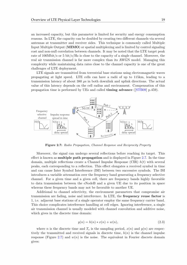
Figure 2.7: Radio Propagation, Channel Response and Reciprocity Property
Moreover, the signal can undergo several reflections before reaching its target. Thiseffect is known as multiple path propagation and is displayed in Figure 2.7. In the timedomain, multiple reflections create a Channel Impulse Response (CIR) h(t) with severalpeaks, each corresponding to a reflection. This effect elongates a received symbol in timeand can cause Inter Symbol Interference (ISI) between two successive symbols. The ISIintroduces a variable attenuation over the frequency band generating a frequency selectivechannel. For a given time and a given cell, there are frequency bands highly favorableto data transmission between the eNodeB and a given UE due to its position in spacewhereas these frequency bands may not be favorable to another UE.
Additional to channel selectivity, the environment parameters that compromise airtransmission are fading, noise and interference. In LTE, the frequency reuse factor is1, i.e. adjacent base stations of a single operator employ the same frequency carrier band.This choice complicates interference handling at cell edges. Ignoring interference, a singleair transmission channel is usually modeled with channel convolution and additive noise,which gives in the discrete time domain:
y(n) = h(n) ∗ x(n) + w(n), (2.3)
where n is the discrete time and Ts is the sampling period, x(n) and y(n) are respec-tively the transmitted and received signals in discrete time, h(n) is the channel impulseresponse (Figure 2.7) and w(n) is the noise. The equivalent in Fourier discrete domaingives:

20 3GPP Long Term Evolution
Y (k) = H(k)X(k) +W (k), (2.4)
where k is the discrete frequency. In order to estimate H(k), known reference signals(also called pilot signals) are transmitted. A reference signal cannot be received at the sametime as the data it is aiding. Certain channel assumptions must be made, including slowmodification over time. The time over which a Channel Impulse Response h(t) remainsalmost constant is called channel coherence time. For a flat Rayleigh fading channelmodel at 2 GHz, modeling coherence time is about 5 millisecond for a UE speed of 20km/h ([STB09] p. 576). The faster the UE moves, the faster the channel changes and thesmaller the coherence time becomes.
The UE velocity also has an effect on radio propagation, due to the Doppler effect.For a carrier frequency of 2.5 GHz and a UE velocity of 130 km/h, the Doppler effectfrequency shifts the signal up to 300 Hz ([STB09] p.478). This frequency shift must beevaluated and compensated for each UE. Moreover, guard frequency bands between UEsare necessary to avoid frequency overlapping and Inter Carrier Interference (ICI).
Figure 2.7 shows a Non-line-of-sight (NLOS) channel, which occurs when the directpath is shadowed. Figure 2.7 also displays the property of channel reciprocity; thechannels in downlink and in uplink can be considered to be equal in terms of frequencyselectivity within the same frequency band. When downlink and uplink share the sameband, channel reciprocity occurs, and so the uplink channel quality can be evaluatedfrom downlink reception study and vice-versa. LTE technologies use channel propertyestimations H(k) for two purposes:
� Channel estimation is used to reconstruct the transmitted signal from the receivedsignal.
� Channel sounding is used by the eNodeBs to decide which resource to allocateto each UE. Special resources must be assigned to uplink channel soundings be-cause a large frequency band exceeding UE resources must be sounded initially byeach UE to make efficient allocation decisions. The downlink channel sounding isquite straightforward, as the eNodeB sends reference signals over the entire downlinkbandwidth.
Radio models describing several possible LTE environments have been developed by3GPP (SCM and SCME models), ITU-R (IMT models) and a project named IST-WINNER.They offer tradeoffs between complexity and accuracy. Their targeted usage is hardwareconformance tests. The models are of two kinds: matrix-based models simulate the propa-gation channel as a linear correlation (equation 2.3) while geometry-based models simulatethe addition of several propagation paths (Figure 2.7) and interferences between users andcells.
LTE is designed to address a variety of environments from mountainous to flat, includ-ing both rural and urban with Macro/Micro and Pico cells. On the other hand, Femtocellswith very small radii are planned for deployment in indoor environments such as homesand small businesses. They are linked to the network via a Digital Subscriber Line (DSL)or cable.
2.3.2 Selective Channel Equalization
The air transmission channel attenuates each frequency differently, as seen in Figure 2.7.Equalization at the decoder site consists of compensating for this effect and reconstructing

Overview of LTE Physical Layer Technologies 21
the original signal as much as possible. For this purpose, the decoder must preciselyevaluate the channel impulse response. The resulting coherent detection consists of 4steps:
1. Each transmitting antenna sends a known Reference Signal (RS) using predefinedtime/frequency/space resources. Additional to their use for channel estimation, RScarry some control signal information. Reference signals are sometimes called pilotsignals.
2. The RS is decoded and the H(f) (Equation 2.4) is computed for the RS time/fre-quency/space resources.
3. H(f) is interpolated over time and frequency on the entire useful bandwidth.
4. Data is decoded exploiting H(f).
The LTE uplink and downlink both exploit coherent detection but employ differentreference signals. These signals are selected for their capacity to be orthogonal with eachother and to be detectable when impaired by Doppler or multipath effect. Orthogonalityimplies that several different reference signals can be sent by the same resource and stillbe detectable. This effect is called Code Division Multiplexing (CDM). Reference signalsare chosen to have constant amplitude, reducing the transmitted Peak to Average PowerRatio (PAPR [RL06]) and augmenting the transmission power efficiency. Uplink referencesignals will be explained in 2.4.3 and downlink reference signals in 2.5.3.
As the transmitted reference signal Xp(k) is known at transmitter and receiver, it canbe localized and detected. The simplest least square estimation defines:
H(k) = (Y (k)−W (k))/Xp(k) ≈ Y (k)/Xp(k). (2.5)
H(k) can be interpolated for non-RS resources, by considering that channel coherenceis high between RS locations. The transmitted data is then reconstructed in the Fourierdomain with X(k) = Y (k)/H(k).
2.3.3 eNodeB Physical Layer Data Processing
Figure 2.8 provides more details of the eNodeB physical layer that was roughly describedin Figure 2.3. It is still a simplified view of the physical layer that will be explained in thenext sections and modeled in Chapter 7.
In the downlink data encoding, channel coding (also named link adaptation)prepares the binary information for transmission. It consists in a Cyclic RedundancyCheck (CRC) /turbo coding phase that processes Forward Error Correction (FEC), a ratematching phase to introduce the necessary amount of redundancy, a scrambling phaseto increase the signal robustness, and a modulation phase that transforms the bits intosymbols. The parameters of channel coding are named Modulation and Coding Scheme(MCS). They are detailed in Section 2.3.5. After channel coding, symbol processingprepares the data for transmission over several antennas and subcarriers. The downlinktransmission schemes with multiple antennas are explained in Sections 2.3.6 and 2.5.4 andthe Orthogonal Frequency Division Multiplexing Access (OFDMA), that allocates data tosubcarriers, in Section 2.3.4.
In the uplink data decoding, the symbol processing consists in decoding Sin-gle Carrier-Frequency Division Multiplexing Access (SC-FDMA) and equalizing signalsfrom the different antennas using channel estimates. SC-FDMA is the uplink broadband

22 3GPP Long Term Evolution
OFDMA Encoding
Downlink Data Encoding
data(bits)
Multi-Antenna PrecodingModulationInterleaving/
ScramblingRate
MatchingCRC/Turbo
Coding
Channel Coding Symbol Processing
Turbo Decoding/CRC
Uplink Data Decoding
data(bits)
Rate Dematching
/HARQ
Descrambling/Deinterleaving
Channel Decoding
DemodulationSC-FDMA Decoding/Multi-Antenna Equalization
Symbol ProcessingChannel Estimation
Figure 2.8: Uplink and Downlink Data Processing in the LTE eNodeB
transmission technology and is presented in Section 2.3.4. Uplink multiple antenna trans-mission schemes are explained in Section 2.4.4. After symbol processing, uplink channeldecoding consists of the inverse phases of downlink channel coding because the chosentechniques are equivalent to the ones of downlink. HARQ combining associates the re-peated receptions of a single block to increase robustness in case of transmission errors.
Next sections explain in details these features of the eNodeB physical layer, startingwith the broadband technologies.
2.3.4 Multicarrier Broadband Technologies and Resources
LTE uplink and downlink data streams are illustrated in Figure 2.9. The LTE uplink anddownlink both employ technologies that enable a two-dimension allocation of resourcesto UEs in time and frequency. A third dimension in space is added by Multiple InputMultiple Output (MIMO) spatial multiplexing (Section 2.3.6). The eNodeB decides theallocation for both downlink and uplink. The uplink allocation decisions must be sentvia the downlink control channels. Both downlink and uplink bands have six possiblebandwidths: 1.4, 3, 5, 10, 15, or 20 MHz.
frequency
between 1.4 and 20MHz
UE1 UE3UE2
12
3
frequency allocation choices
(a) Downlink: OFDMA
frequency
123
UE1 UE3UE2
between 1.4 and 20MHz
frequency allocation choices
(b) Uplink: SC-FDMA
Figure 2.9: LTE downlink and uplink multiplexing technologies

Overview of LTE Physical Layer Technologies 23
Broadband Technologies
The multiple subcarrier broadband technologies used in LTE are illustrated in Figure2.10. Orthogonal Frequency Division Multiplexing Access (OFDMA) employed for thedownlink and Single Carrier-Frequency Division Multiplexing (SC-FDMA) is used forthe uplink. Both technologies divide the frequency band into subcarriers separated by15 kHz (except in the special broadcast case). The subcarriers are orthogonal and dataallocation of each of these bands can be controlled separately. The separation of 15 kHzwas chosen as a tradeoff between data rate (which increases with the decreasing separation)and protection against subcarrier orthogonality imperfection [R1-05]. This imperfectionoccurs from the Doppler effect produced by moving UEs and because of non-linearitiesand frequency drift in power amplifiers and oscillators.
Both technologies are effective in limiting the impact of multi-path propagation on datarate. Moreover, the dividing the spectrum into subcarriers enables simultaneous access toUEs in different frequency bands. However, SC-FDMA is more efficient than OFDMA interms of Peak to Average Power Ratio (PAPR [RL06]). The lower PAPR lowers the costof the UE RF transmitter but SC-FDMA cannot support data rates as high as OFDMAin frequency-selective environments.
Serial to parallelsize M (1200)
IFFTsize N(2048)
0
0
0
Insert CP
size C(144)
Downlink OFDMA Encoding
Freq. Mapping
DFTsize M
(60)
IFFTsize N(2048)
Insert CP
size C(144)
Uplink SC-FDMA Encoding
energy
time
frequency
M complex values (1200) to send to U
users
energy
time
frequency
...
M complex values (60) to send to
the eNodeB
...
... ...
CP
CP
... ...
CP
CP
1symbol
1symbol
M subcarriers
M subcarriers
0
0
0
Freq. Mapping
0
Figure 2.10: Comparison of OFDMA and SC-FDMA
Figure 2.10 shows typical transmitter implementations of OFDMA and SC-FDMAusing Fourier transforms. SC-FDMA can be interpreted as a linearly precoded OFDMAscheme, in the sense that it has an additional DFT processing preceding the conventionalOFDMA processing. The frequency mapping of Figure 2.10 defines the subcarrier accessedby a given UE.
Downlink symbol processing consists of mapping input values to subcarriers by per-forming an Inverse Fast Fourier Transform (IFFT). Each complex value is then transmittedon a single subcarrier but spread over an entire symbol in time. This transmission schemeprotects the signal from Inter Symbol Interference (ISI) due to multipath transmission. Itis important to note that without channel coding (i.e. data redundancy and data spreadingover several subcarriers), the signal would be vulnerable to frequency selective channelsand Inter Carrier Interference (ICI). The numbers in gray (in Figure 2.10) reflect typicalparameter values for a signal of bandwidth of 20 MHz. The OFDMA encoding is processedin the eNodeB and the 1200 input values of the case of 20MHz bandwidth carry the dataof all the addressed UEs. SC-FDMA consists of a small size Discrete Fourier Transform

24 3GPP Long Term Evolution
(DFT) followed by OFDMA processing. The small size of the DFT is required as thisprocessing is performed within a UE and only uses the data of this UE. For an example of60 complex values the UE will use 60 subcarriers of the spectrum (subcarriers are shownlater to be grouped by 12). As noted before, without channel coding, data would be proneto errors introduced by the wireless channel conditions, especially because of ISI in theSC-FDMA case.
Cyclic Prefix
The Cyclic Prefix (CP) displayed in Figures 2.10 and 2.11 is used to separate two succes-sive symbols and thus reduces ISI. The CP is copied from the end of the symbol data toan empty time slot reserved before the symbol and protects the received data from timingadvance errors; the linear convolution of the data with the channel impulse response isconverted into a circular convolution, making it equivalent to a Fourier domain multiplica-tion that can be equalized after a channel estimation (Section 2.3.2). CP length in LTE is144 samples = 4.8µs (normal CP) or 512 samples = 16.7µs in large cells (extended CP).A longer CP can be used for broadcast when all eNodeBs transfer the same data on thesame resources, so introducing a potentially rich multi-path channel. Generally, multipathpropagation can be seen to induce channel impulse responses longer than CP. The CPlength is a tradeoff between the CP overhead and sufficient ISI cancellation [R1-05].
CP 1 symbol (2048 complex values)
...160 144 144 144 144 144 144 160
1 slot = 0.5 ms = 7 symbols (with normal CP) = 15360 complex values
Figure 2.11: Cyclic Prefix Insertion
Time Units
Frequency and timing of data and control transmission is not decided by the UE. TheeNodeB controls both uplink and downlink time and frequency allocations. The allocationbase unit is a block of 1 millisecond per 180kHz (12 subcarriers). Figure 2.12 shows 2 PRBs.A PRB carries a variable amount of data depending on channel coding, reference signals,resources reserved for control...
Certain time and frequency base values are defined in the LTE standard, which al-lows devices from different companies to interconnect flawlessly. The LTE time units aredisplayed in Figure 2.12:
� A basic time unit lasts Ts = 1/30720000s ≈ 33ns. This is the duration of 1complex sample in the case of 20 MHz bandwidth. The sampling frequency is thus30.72MHz = 8∗3.84MHz, eight times the sampling frequency of UMTS. The choicewas made to simplify the RF chain used commonly for UMTS and LTE. Moreover, asclassic OFDMA and SC-FDMA processing uses Fourier transforms, symbols of sizepower of two enable the use of FFTs and 30.72MHz = 2048∗15kHz = 211 ∗15kHz,with 15kHz the size of a subcarrier and 2048 a power of two. Time duration for allother time parameters in LTE is a multiple of Ts.

Overview of LTE Physical Layer Technologies 25
� A slot is of length 0.5millisecond = 15360Ts. This is also the time length of a PRB.A slot contains 7 symbols in normal cyclic prefix case and 6 symbols in extended CPcase. A Resource Element (RE) is a little element of 1 subcarrier per one symbol.
� A subframe lasts 1millisecond = 30720Ts = 2slots. This is the minimum durationthat can be allocated to a user in downlink or uplink. A subframe is also calledTransmission Time Interval (TTI) as it is the minimum duration of an independentlydecodable transmission. A subframe contains 14 symbols with normal cyclic prefixthat are indexed from 0 to 13 and are described in the following sections.
� A frame lasts 10millisecond = 307200Ts. This corresponds to the time required torepeat a resource allocation pattern separating uplink and downlink in time in caseof Time Division Duplex (TDD) mode. TDD is defined below.
subcarrier spacing 15kHz
1 frame =10ms
frequency
time
1 PRB
1 slot=0.5ms = 7 symbols
1 subframe=1ms
12 subcarriers 180kHz 1 PRB
Bandwidth = between 6 RBs (1.4MHz band) and 100 RBs (20MHz band)
1 RE
Figure 2.12: LTE Time Units
In the LTE standard, the subframe size of 1 millisecond was chosen as a tradeoffbetween a short subframe which introduces high control overhead and a long subframewhich significantly increases the retransmission latency when packets are lost [R1-06b].Depending on the assigned bandwidth, an LTE cell can have between 6 and 100 resourceblocks per slot. In TDD, special subframes protect uplink and downlink signals from ISIby introducing a guard period ([36.09c] p. 9).
Duplex Modes
Figure 2.13 shows the duplex modes available for LTE. Duplex modes define how thedownlink and uplink bands are allocated respective to each other. In Frequency DivisionDuplex (FDD) mode, the uplink and downlink bands are disjoint. The connection is thenfull duplex and the UE needs to have two distinct Radio Frequency (RF) processing chainsfor transmission and reception. In Time Division Duplex (TDD) mode, the downlink andthe uplink alternatively occupy the same frequency band. The same RF chain can thenbe used for transmitting and receiving but available resources are halved. In Half-DuplexFDD (HD-FDD) mode, the eNodeB is full duplex but the UE is half-duplex (so can havea single RF chain). In this mode, separate bands are used for the uplink and the downlinkbut are never simultaneous for a given UE. HD-FDD is already present in GSM.
ITU-R defined 17 FDD and 8 TDD frequency bands shared by LTE and UMTS stan-dards. These bands are located between 698 and 2690 MHz and lead to very differentchannel behavior depending on carrier frequency. These differences must be accounted for

26 3GPP Long Term Evolution
frequency
time time time
FDD TDD HD-FDDUE1 UE2 UE1 UE2
UE1 UE2 UE1UE2
frequency frequency
downlinkuplink
Figure 2.13: Different types of LTE duplex modes
during the calibration of base stations and UEs. The following Sections will focus on FDDmode.
2.3.5 LTE Modulation and Coding Scheme
Within a single LTE cell, a given UE can experience different Signal-to-Interference plusNoise Ratio (SINR) depending on the radio properties of its environment: the distanceof the base station antenna, the base station emission power, the interference of otherusers, the number of diversity antennas, and so on Several LTE channel coding featuresare created in order to obtain data rates near channel capacity in every situation. Channelcoding operations are usually very computationally complex operations, and parametersfor optimization must be chosen with care. For the case of one antenna port, two LTEphysical layer parameters can be modified to maximize the throughput. These parametersare called Modulation and Coding Scheme (MCS):
� The channel coding rate is a parameter which determines the amount of redun-dancy to add in the input signal to allow Forward Error Correction (FEC) processing.A higher redundancy leads to more robust signal at the cost of throughput.
� The modulation scheme refers to the way data symbols are associated to a set oftransmit bits. A symbol is a complex value that is used to modulate a carrier for airtransmission. Three schemes are available in LTE: QPSK, 16-QAM and 64-QAM.They associate 2, 4 and 6 bits respectively to a single symbol and this number ofbits is the modulation level. Of the three modulation schemes, QPSK is the mostrobust for transmission errors but 64-QAM allows the highest throughput ([36.09c]p.79).
The downlink channel quality estimation required for downlink MCS scheme choiceis more complex than for its uplink equivalent. However, the report of downlink channelquality is vital for the eNodeB when making downlink scheduling decisions. In FDDmode, no reciprocity of frequency selective fading between uplink and downlink channelscan be used (Section 2.3.1). The UE measures downlink channel quality from downlinkreference signals and then reports this information to its eNodeB. The UE report consistsof a number between 0 and 15, generated by the UE, representing the channel capacityfor a given bandwidth. This number is called CQI for Channel Quality Indicatorand is sent to the eNodeB in the uplink control channel. The CQI influences the choiceof resource allocation and MCS scheme. In Figure 2.14(a), the channel coding rate andmodulation rate are plotted against CQI, and the global resulting coding efficiency. Itmay be seen that the coding efficiency can be gradually adapted from a transmission rateof 0.15 bits/resource element to 5.55 bits/resource element.
CQI reports are periodic, unless the eNodeB explicitly requests aperiodic reports. Pe-riodic reports pass through the main uplink control channel known as the Physical UplinkControl CHannel (PUCCH, Section 2.4.2). When PUCCH resources are unavailable, the

Overview of LTE Physical Layer Technologies 27
reports are multiplexed in the uplink data channel known as the Physical Uplink SharedCHannel (PUSCH, Section 2.4.2). Aperiodic reports are sent in the PUSCH when ex-plicitly requested by the eNodeB. Periodic CQI reports have a period between 2 and 160millisecond. Periodic CQI reports contain one CQI if no spatial multiplexing is used ortwo CQI (one per rank) in the case of rank 2 downlink spatial multiplexing (Section 2.3.6).Aperiodic CQI modes exist including one CQI for the whole band and possibly an addi-tional CQI for a set of preferred subbands ([36.09e] p.37). The choice of following theUE recommendation is given to the eNodeB. After receiving the UE report, the eNodeBsends data using the downlink data channel known as the Physical Downlink Shared Chan-nel (PDSCH, Section 2.5.2). Control values are simultaneously transmitting in the maindownlink control channel known as the Physical Downlink Control Channel (PDCCH,Section 2.5.2). These PDCCH control values carry Downlink Control Information (DCI)which include the chosen MCS scheme, HARQ parameters.
Figure 2.14(b) shows the effect of MCS on the throughput of a LTE transmission usinga single antenna, a bandwidth of 1.4MHz, no HARQ and one UE. With only one UE inthe cell, there can be no interference, so SINR is equal to SNR (Signal-to-Noise Ratio).The results were generated by the LTE simulator of Vienna University of Technology witha Additive White Gaussian Noise (AWGN) channel model and published in [MWI+09].It may be seen that, for the studied channel model, a throughput close to the channelcapacity can be achieved if the link adaptation is well chosen. It may also be noted thatthis choice is very sensitive to the SNR.
0
0.2
0.4
0.6
0.8
1
Cha
nnel
cod
ing
rate
0 5 10 150
1
2
3
4
5
6
CQI value
bit p
er s
ymbo
l
Efficiency
Modulationlevel
64 -QAM
16 -QAM
QPSK
(a) Link Adaptation Parametersfor each CQI
-20 -10 0 10 20012345678
SNR [dB]
thro
ughp
ut [M
bit/
s]
CQIs 10-15, 64-QAM
CQIs 7-9, 16-QAM
CQIs 1-6, QPSK
system capacity
(b) Link Adaptation Effect on theThroughput of a 1.4 MHz Cell
Figure 2.14: LTE Link Adaptation
The techniques used to add redundancy and process Forward Error Correction (FEC)are different for control and data channels. The majority of control information in thePDCCH and the PUCCH use tail biting convolutional coding, sequence repetition andpruning while data channels (PDSCH, PUSCH) use turbo coding, sequence repetition andpruning ([Rum09] p.76).
The convolutional code used for control in LTE (Figure 2.15(a)) has a 1/3 rate i.e.the code adds 2 redundant bits for each information bit. The encoder was chosen for itssimplicity to allow to easier PDCCH decoding by UEs. Indeed, a UE needs to permanentlydecode many PDCCH PRBs, including many that are not intended for decoding and sothis permanent computation must be limited. Convolutional coding is well suited for aFEC system with small blocks because it is not necessary to start in a predefined state.Moreover, convolutional codes can be efficiently decoded using a Viterbi decoder [CS94].The absence of predefined state is important because a predefined starting state has a cost

28 3GPP Long Term Evolution
in the encoded stream. Instead, the 6 last bits of the encoded sequence serve as startingstate of the encoder, transforming a linear convolution into a circular convolution, in thesame way as the Cyclic Prefix with the channel impulse response. This technique is namedtail biting.
dn dn-1 dn-2 dn-3 dn-4 dn-5
d0d1d2...n bits
n bitsn bitsn bits
initialization values
(a) Convolutional encoder used for control
ΠΠ-1
n bits
n systematic bits
Π
D2
D1
Π
Possible iterative turbo decoderLTE turbo encoder
n LLRs
n parity bits
E1
E2
n parity bits
(b) Turbo code used for data
Figure 2.15: LTE Forward Error Correction methods
A turbo code [BG07] in LTE (Figure 2.15(b)) introduces redundancy in all LTEtransmitted data. It has a rate of 1/3 and consists of an interleaver and two identical rate-1 convolutional encoders E1 and E2. One convolutional encoder (E1) processes the inputdata while the other convolutional encoder (E2) processes a pseudo-randomly interleavedversion of the same data. The turbo coder outputs a concatenation of its unmodifiedinput (systematic bits) and the two convoluted signals (parity bits). The resulting outputfacilitates FEC because there is little probability of having a low Hamming weight (numberof 1s in the bit stream), thus improving detection. Each Code Block is independently turbocoded. A Code Block size ranges from 40 to 6144 bits (Section 2.2.3). Turbo coding isvery efficient for long Code Blocks but it necessitates 12 tail bits containing no informationthat reduce its efficiency for small blocks.
Turbo coding and decoding are two of the most demanding functions of the LTEphysical layer. Special coprocessors for turbo coding and decoding are included in multi-core architectures intended to handle eNodeB physical layer computation. Turbo iterativedecoders ([Pyn97] and Figure 2.15(b)) contain two convolution decoders that calculatethe A Posteriori Probability (APP) of their input. At each iteration of the decoder, thedetection belief of the decoded bit increases. APPs are stored in Log Likelihood Ratio(LLR) integer values where the sign indicates the detected binary value (0 or 1) andthe amplitude indicates the reliability of the detection. For each bit, the turbo decoderoutputs an LLR. Such a decoder, manipulating not only raw bits but also detection belief,is called soft decision decoder. For the possibility of HARQ retransmissions, LLR valuesof preceding receptions are stored to allow the combination of the preceding with the newreception. This combining operation can increase the signal to noise ratio in a code blockand hence increase the odds for a successful decoding by the Turbo decoder.
After convolutional or turbo coding, the bits enter a circular Rate Matching (RM)process where they are interlaced, repeated and pruned to obtain the desired coding rate(Figure 2.14(a)) with an optimal amount of spread redundancy.
Hybrid Automatic Repeat reQuest
HARQ retransmission of lost blocks is a part of link adaptation. HARQ introduces redun-dancy in the signal to counteract the channel impairments. Moreover, HARQ is hybridin the sense that each retransmission can be made more robust by a stronger modulationand by stronger channel coding.

Overview of LTE Physical Layer Technologies 29
An eNodeB has 3 milliseconds after the end of a PUSCH subframe reception to processthe frame, detect a possible reception error via Cyclic Redundancy Check (CRC) decodingand send back a NACK bit in the PDCCH. The uplink HARQ is synchronous in that aretransmission, if any, always appears 8 millisecond after the end of the first transmission.This fixed retransmission scheme reduces signaling in PUCCH. The repetitions can beadaptive (each one with a different MCS scheme), or not.
Downlink HARQ is consistently asynchronous and adaptive. There is at least 8 mil-lisecond between two retransmissions of a Transport Block. It introduces more flexibilitythan the uplink scheme at the cost of signaling.
When a Transport Block is not correctly received, 8 different stop-and-wait processesare enabled, for both downlink and uplink receivers. This number of processes reduces therisk of the communication being blocked while waiting for HARQ acknowledgement, withthe cost of memory to store the LLRs for each process (Section 2.3.5). Data from severalrepetitions are stored as LLRs and recombined, making HARQ hybrid.
2.3.6 Multiple Antennas
In LTE, eNodeBs and UEs can use several antennas to improve the quality of wirelesslinks:
� eNodeB baseband processing can generate up to 4 separate downlink signals. Eachsignal is allocated to an antenna port. The eNodeB can also receive up to 4 differentuplink signals. Two antennas sending the same signal are processed at the basebandprocessing as a single antenna port.
� A UE can have 2 receive antennas and receive 2 different signals simultaneously. Itcan have 2 transmit antennas but the UE will switch between these antennas as ithas only one RF amplifier,.
Multiple transmit antennas (NT > 1), receive antennas (NR > 1) or both can improvelink quality and lead to higher data rates with higher spectral efficiency. For a preciseintroduction to MIMO channel capacity, see [Hol01]. Different multiple antenna effectscan be combined:
� Spatial diversity (Figure 2.16(a)) consists of using different paths between antennasets to compensate for the selective frequency fading of channels due to multipathtransmission. There are two modes of spatial diversity: transmission or reception.Transmission spatial diversity necessitates several transmit antennas. Combiningseveral transmit antennas consists in choosing the right way to distribute data overseveral antennas. A common technique is named Space-Time Block Coding (STBC)where successive data streams are multiplexed in the channels and made as orthogo-nal as possible to enhance the reception diversity. The most common of these codesis Alamouti; it offers optimal orthogonality for 2 transmit antennas [Ala07]. No suchoptimal code exists for more than 2 antennas. Reception spatial diversity (Figure2.16(a)) uses several receive antennas exploiting the diverse channels, by combiningtheir signal with Maximal-Ratio Combining (MRC).
� Spatial multiplexing gain, sometimes called MIMO effect is displayed in Figure2.16(b) for the case NT = NR = 2. It consists of creating several independentchannels in space, exploiting a good knowledge of the channels and reconstructingthe original data of each channel. MIMO can increase the throughput by a factor

30 3GPP Long Term Evolution
of min(NT , NR) but this factor is never obtained in real life because multiple pathsare never totally uncorrelated and channel estimation requires additional referencesignals. MIMO actually takes advantage of the multipath scattering that spatialdiversity tries to counteract.
� Beamforming, also called array gain, consists of creating constructive and de-structive interference of the wavefront to concentrate the signal in a given spatialdirection. This is displayed in Figure 2.16(c). These interferences are generated byseveral transmitting antennas precoded by factors named beam patterns.
freq.
freq.
freq.
freq.
MRC
(a) Spatial Diversity
h00
h10 h01
h11
y0
y1
y0 = h00 * x0 + h01 * x1y1 = h10 * x0 + h11 * x1
If the channels are known and independant, x0 and x1 can be computed
x0
x1
Y = H X
(b) Spatial Multiplexing
eNodeB
(c) Beam Forming
Figure 2.16: LTE link adaptation
Without spatial multiplexing, every PRB corresponding to a single UE has the sameMCS. In downlink spatial multiplexing mode, two separate MCS can be used for twodifferent Transport Blocks sent simultaneously to a UE. A more complex scheme wasshown to greatly increase the control with only slightly higher data rates [R1-06a].
2.4 LTE Uplink Features
2.4.1 Single Carrier-Frequency Division Multiplexing
Uplink Pilot Signals
The SC-FDMA presented earlier is also known as DFTS-OFDM (DFT-Spread OrthogonalFrequency Division Multiplexing). A discussion on uplink technology choices can be foundin [CMS06]. A SC-FDMA decoder in the eNodeB necessitates a channel estimation toequalize the received signal. This channel estimation is performed sending Zadoff-Chu(ZC) sequences known to both the UE and the eNodeB. ZC sequences will be explained inSection 2.4.3. These sequences are called Demodulation Reference Signals (DM RS) andare transmitted on the center symbol of each slot (Figure 2.17). The eNodeB also needsto allocate uplink resources to each UE based on channel frequency selectivity, choosing

LTE Uplink Features 31
frequency bands that are most favorable to the UE. DM RS are only sent by a UE in itsown frequency band; they do not predict if it is necessary to allocate new frequencies inthe next subframe. This is the role of Sounding Reference Signal (SRS). The positions ofDM RS and SRS in the uplink resource blocks is illustrated in Figure 2.17.
UE1 PUSCHUE1 sounding signalUE2 PUSCHUE2 sounding signalReference signalno emission
UE1
UE2
01
23
45
67
8910
1112
130
12
34
56
78
910
1112
1301
23
45
67
8910
1112
13
1 PRB allocated
2 PRBs allocated
symbol number
Figure 2.17: Reference Signals location in the uplink resources
DM RS are located in symbols 3 and 10 of each subframe. When explicitly requested bythe eNodeB, SRS signals of ZC sequences are sent in the in symbol 13 location. The SRS fora given UE is located every 2 subcarriers using the Interleaved FDMA (IFDMA) method.A 10-bit PDCCH message describes the time, period (between 2 and 320 millisecond) andbandwidth for the UE to send the SRS message. For more details on SRS, see [STB09]p.370. As both DM RS and SRS are Constant Amplitude Zero AutoCorrelation (CAZAC)sequences, two UEs can send each their SRS using the same resources provided they usedifferent cyclic shifts, making sequences orthogonal (Section 2.4.3). The eNodeB is thenable to separate the two different pilot signals. Figure 2.17 displays an example of threesubframes with UE 1 transmitting data on one fixed PRB with a SRS cycle of more than2 millisecond and UE 2 sending data on two fixed PRBs with a SRS cycle of 2 millisecond.
2.4.2 Uplink Physical Channels
Uplink data and control streams are sent using three physical channels allocated on thesystem bandwidth:
� The Physical Uplink Shared Channel (PUSCH) carries all the data sent betweena eNodeB and its UEs. It can also carry some control. LTE PUSCH only supportslocalized UE allocations, i.e. all PRBs allocated to a given UE are consecutive infrequency.
� The Physical Uplink Control Channel (PUCCH) carries the major part of thetransmitted control values via uplink.
� Physical Random Access Channel (PRACH) carries the connection requestsfrom unconnected UEs.
Figure 2.18 illustrates the localization of the physical channels for the example of a 5MHz cell. The PUCCH is localized on the edges of the bandwidth while PUSCH occupiesmost of the remaining PRBs. PUCCH information with redundancy is sent on pairs ofPRBs called regions (indexed in Figure 2.18), where the two PRBs of a region are located

32 3GPP Long Term Evolution
on opposite edges. This technique is called frequency hopping and protects the PUCCHagainst localized frequency selectivity. There are typically 4 PUCCH regions per 5 MHzband. However, the eNodeB can allocate the PUSCH PRBs in PUCCH regions if they arenot needed for control. Multiple UE control values can be multiplexed in PUCCH regionsvia Code Division Multiplexing (CDM).
UE1
UE2
5 MHz Cell25 PRBs = 300 subcarriersTypical Case with 4 PUCCH Regions (PRB pairs 0 to 3)
0 12 3
3 21 0
0 12 3 0 1
2 30 12 3
3 21 0
3 21 0
3 21 0
PUCCH PRBs
PUCCH PRBs
PUSCH PBRs
PRB FrequencyHopping of 12 subcarriers
subframe
UE1 PUSCHUE2 PUSCHReference SignalNo EmissionPRACH type 0 BurstShared PUCCH
Figure 2.18: Uplink Channels
Uplink decisions are generally taken by the eNodeB MAC scheduler and transmittedvia downlink control channels. Consequently, the UEs are not required to send back theseeNodeB decisions to the eNodeB, thus reducing the overhead of the PUCCH. 7 PUCCHregion formats are defined according to the kind of information carried. The PUCCHcontains the requests for more uplink data resources via an uplink Scheduling Request bit(SR), and the Buffer Status Reports (BSR) signals the amount of pending data from theUE PUSCH to the eNodeB. The PUCCH also signals the UE preferences for downlinkModulation and Coding Scheme (MCS, Section 2.3.5) including:
� Hybrid Automatic Repeat reQuest (HARQ), Acknowledgement (ACK), or NonAcknowledgement (NACK) are stored in 1 or 2 bits and require HARQ retransmis-sions if data was lost and the Cyclic Redundancy Check (CRC) was falsely decoded.
� A Channel Quality Indicator (CQI, Section 2.3.5) consists of 20 bits transportingindicators of redundancy 1 or 2 which recommend a MCS to the eNodeB for eachtransmitted Transport Block.
� MIMO Rank Indicator (RI) and Precoding Matrix Indicator (PMI) bitswhich recommend a multiple antenna scheme to the eNodeB (Section 2.3.6).
The PUCCH carries this control information periodically. If PRB is unavailable in thePUCCH, the PUSCH can carry some control information. Additionally, the eNodeB canrequest additional aperiodic CQI and link adaptation reports. These reports are sent inPUSCH and can be much more complete than periodic reports (up to 64 bits).
The PRACH is allocated periodically over 72 subcarriers (6 PRBs, Figure 2.18). Em-ploying 72 subcarriers is favorable because it has the widest bandwidth available for allLTE configurations between 1.4 MHz and 20 MHz. The PRACH burst can last between 1and 3 subframes depending on the chosen mode; long modes are necessary for large cells.The PRACH period depends on the adjacent cell configurations and is typically severalsubframes. See Section 2.4.5 and [STB09] p.421 for more details on the PRACH.

LTE Uplink Features 33
The uplink is shared between several transmitting UEs with different velocities anddistances to the eNodeB. Certain precautions must be taken when multiple UEs are trans-mitting simultaneously , one of which is the timing advance. Timing advance consists ofsending data with the corrected timing, so compensating for the propagation time and al-lowing the synchronization of all data received at the eNodeB. The correct timing advanceis evaluated using the timing received from the PRACH bursts.
2.4.3 Uplink Reference Signals
In uplink communication, a Demodulation Reference Signal (DM RS) is constructed from aset of complex-valued Constant Amplitude Zero AutoCorrelation (CAZAC) codes knownas Zadoff-Chu (ZC) sequences [Chu72] [Pop92]. ZC sequences are computed with theformula:
zq(n) = exp(−jπqn(n+ 1)
NZC) (2.6)
where n is the sample number, q is the sequence index ranging from 1 to NZC − 1,and NZC is the sequence size. Three ZC sequences of length 63 with indexes 25, 29 and34 are illustrated in Figure 2.19. Their amplitude and the amplitude of their Fouriertransform are constant, keeping low the PAPR of their transmission (Figure 2.19(a)). Allthree sequences have an autocorrelation close to the Dirac function, enabling the creationof several orthogonal sequences from a single sequence using cyclic shifts. It may also benoted that the cross correlation between two ZC sequences with different indices is smallcompared to the autocorrelation peak (Figure 2.19(b)). Consequently, two sequences canbe decoded independently when sent simultaneously as long as their indices or cyclic shiftsare different.
-30 -20 -10 0 10 20 30-1
-0.50
0.51
(a) ZC Sequences Real and Imaginary Parts
-60 -20 0 20 600102030405060
0102030405060
-60 -20 0 20 60
“Perfect” autocorrelations
Reduced intercorrelations
zc25zc29zc34
zc25 o zc29zc29 o zc34zc34 o zc25
(b) ZC Sequences Auto and Crosscorrelationmagnitudes
Figure 2.19: Length-63 Zadoff-Chu Sequences with index 25, 29 and 34
Each uplink DM RS of length NP consists of a ZC sequence with the highest primesize smaller than NP . The ZC sequence is cyclically extended to NP elements and thencyclically shifted by α elements. For the smallest DM RS sizes of 12 and 24 elements,special codes replace ZC sequences because they outperform the ZC sequences in thesecases ([STB09] p.361). DM RS primarily serve to estimate the channel. They also carryinformation in their sequence index q and cyclic shift α, namely an ID to determine whichdestination eNodeB of the DM RS and to identify the transmitting UE for the case ofMulti-User MIMO (MU-MIMO, Section 2.4.4). Indices and shifts are vital in preventingUEs and cells from interfering with each other.

34 3GPP Long Term Evolution
ZC sequences are used elsewhere in LTE systems, in particular as Sounding ReferenceSignal (SRS, 2.5.5) and in random access procedure (Section 2.4.5).
2.4.4 Uplink Multiple Antenna Techniques
In the first release of LTE, UEs were limited to one transmission amplifier. Uplink single-user spatial multiplexing is thus not possible but multiple UE antennas can still be ex-ploited for better system throughput. Firstly, UEs can optionally have two transmit an-tennas and switch between them depending on the channel quality. This method known asantenna selection necessitates one SRS signal per antenna to report on channel quality.This increase in diversity must be weighed against the cost of this additional SRS signalin overhead
Secondly, reception spatial diversity (Section 2.3.6) is often exploitable becausethe majority of eNodeBs have several receive antennas, each of which have known channelresponses hi. Naming the received values:
y = hx, (2.7)
where each antenna stream has already been equalized (Section 2.3.2) and thus h =[h1h2...hN ]T is the vector of channel responses, each being a scalar and x = [x1x2...xN ]T
and y = [y1y2...yN ]T are the transmitted and received signal vectors across N antennas.The MRC detected signal is given by:
x =hHy
hHh(2.8)
where x is the complex detected symbol. MRC favors antennas which can receive highpower signals. .
Thirdly, Multi-User MIMO (MU-MIMO) also called Spatial Division Multiple Ac-cess (SDMA) consists of allocating the same resources to 2 UEs in the eNodeB and usingthe channel differences in frequency selectivity between UEs to separate the signals whiledecoding. Using MIMO can greatly increase the data rate and only requires special pro-cessing in the eNodeB. It necessitates orthogonal uplink DM RS reference sequences withdifferent cyclic shift to independently evaluate the channel of each UE. Eight different DMRS cyclic shifts are defined in LTE for this purpose. This scheme is often called VirtualMU-MIMO because no added complexity is required at the UE: it is not necessary for theUE to know it shares the same resources with another UE. The complexity increases onlyat eNodeB side.
A 2x2 MU-MIMO scheme is equivalent to that shown in Figure 2.16(b) but with thetransmit antennas connected to separate UEs. Spatial multiplexing decoding, also knownas MIMO detection, consists of reconstructing an estimate vector x of the sent signal vectorx from y and H (Figure 2.16(b)) in the eNodeB. The four channels in H can be consideredto be flat fading (not frequency selective) because they have been individually equalizedupon reception (Section 2.3.2); the channel is thus constant over all SC-FDMA subcarriers.The two most common low complexity linear MIMO detectors are that of Zero Forcing(ZF) and of Minimum Mean-Square Error (MMSE). In the ZF method, where x = Gyis the vector of detected symbols and y is the vector of received symbols, G is computedas the pseudo inverse of H:
G = (HHH)−1HH . (2.9)

LTE Uplink Features 35
The ZF method tends to amplify the transmission noise. The MMSE method is asolution to this problem, with:
G = (HHH + σ2I)−1HH . (2.10)
where σ2 is the estimated noise power and I the identity matrix. Many advancedMIMO decoding techniques [Lar09] [Tre04] exist, notably including Maximum LikelihoodReceiver (MLD) and Sphere Decoder (SD).
2.4.5 Random Access Procedure
The random access procedure is another feature of the uplink. While preceding featuresenabled high performance data transfers from connected UEs to eNodeBs, the randomaccess procedure connects a UE to a eNodeB. It consists of message exchanges initiatedby an uplink message in the PRACH channel (Section 2.4.2). It has two main purposes:synchronizing the UE to the base station and scheduling the UE for uplink transmission.The random access procedure enables a UE in idle mode to synchronize to a eNodeB andbecome connected. It also happens when a UE in connected mode needs to resynchronizeor to perform a handover to a new eNodeB. The scheduling procedures uses the MME(Section 2.2.1) which is the network entity managing paging for phone calls. When aphone call to a given UE is required, the MME asks the eNodeBs to send paging messageswith the UE identity in the PDCCH. The UE monitors the PDCCH regularly even in idlemode. When paging is detected, it starts a random access procedure. The random accessprocedure starts when the UE sends a PRACH signal.
Special time and frequency resources are reserved for the PRACH. Depending on thecell configuration, a PRACH can have a period from 1 to 20 milliseconds. The signal hasseveral requirements. One is that an eNodeB must be able to separate signals from severalUEs transmitted in the same allocated time and frequency window. Another constraint isthat the eNodeB must decode the signal rapidly enough to send back a Random AccessResponse (RAR) in PDSCH. A typical time between the end of PRACH reception andRAR is 4 millisecond ([STB09] p.424). The PRACH message must also be well protectedagainst noise, multipath fading and other interference in order to be detectable at celledges. Finally, the resources dedicated to PRACH must induce a low overhead.
The chosen PRACH signals are ZC sequences of length 839, except in the special TDDformat 4, which is not treated here. Good properties for ZC sequences are explained inSection 2.4.3 where their use in reference signals is described. A set of 64 sequences (calledsignatures) is attributed to each cell (out of 838 sequences in total). A signature is a couple(nS , nCS) where nS ≤ NS ≤ 64 is the root index and nCS ≤ NCS ≤ 64 is the cyclic shift sothat NCS = d64/NSe. A combination of a root and a cyclic shift gives a unique signatureout of 64. A tradeoff between a high number of roots and a high number of cyclic shiftsmust be made. It will be seen that for more cyclic shifts, the easier the decoding becomes(Section 7.3). Each eNodeB broadcasts the first of its signatures and the other signaturesare deduced by the UE from a static table in memory ([36.09c] p.39). A UE sends aPRACH message, by sending one of the 64 signatures included in the eNodeB signatureset.
A PRACH message occupies 6 consecutive PRBs, regardless of the cell bandwidth,during 1 to 3 subframes. This allocation is shown in Figure 2.18. A UE sends PRACHmessages without knowing the timing advance. A Cyclic Prefix (CP) large enough to coverthe whole round trip must be used to protect the message from ISI with previous symbol. Aslightly bigger Guard Time (GT) with no transmission must also be inserted after sending

36 3GPP Long Term Evolution
the PRACH message to avoid ISI with next symbol. GT must be greater than the sum ofround trip and maximum delay spread to avoid overlap between a PRACH message andthe subsequent signal. Depending on the cell size, the constraints on CP and GT sizes aredifferent. Five modes of PRACH messages exist allowing adaption to the cell configuration([36.09e] p.31). The smallest message consists of the 839 samples of one signature sent inone subframe over 800µs = 30720 ∗ 0.8TS = 24576TS with CP and GP of about 100 µ s.This configuration works for cells with a radius under 14 km and thus a round trip timeunder 14 ∗ 2/300000 = 93µs. The longest message consists of 1697 samples (twice the 839samples of one signature) sent in 3 subframes over 1600µs = 30720 ∗ 1.6TS = 49152TSwith CP and GP of about 700 µ s. This configuration is adapted to cells with a radius upto 100 km and thus a round trip time up to 100 ∗ 2/300000 = 667µs.
In 100 km cells, the round trip time can be almost as long as the transmitted signature.Thus no cyclic shift can be applied due to the ambiguity when receiving the same rootwith different cyclic shifts: the signal could result from separate signatures or from UEswith different round trips. The smaller the cell is, the more cyclic shifts can be used forone root resulting in a less complex decoding process and greater orthogonality betweensignatures (see auto and intercorrelations in Figure 2.19(b)).
In the frequency domain, the six consecutive PRBs used for PRACH occupy 6∗0.180 =1.08MHz. The center band of this resource is used to send the 839 signature samplesseparated by 1.25kHz. When the guard band is removed from the signal, it may be seenthat the actual usable band is 839 ∗ 1.25 = 1048.75MHz.
Two modes of random access procedure exist: the most common is the contention-based mode in which multiple UEs are permitted to send a PRACH signal in the sameallocated time and frequency window. Contention-free mode is the other possibility andfor this case, the eNodeB ensures that only a single UE can send a given ZC sequence fora given time and frequency window. The contention-free mode will not be presented here;see [STB09] for more details.
UE eNodeB
Random Access Preamble
Random Access Response
L2/L3 message
Message for early contention resolution
Figure 2.20: Contention-Based Random Access Procedure.
Figure 2.20 illustrates the contention-based random access procedure. Within theUE, the physical layer first receives a PRACH message request from upper layers witha PRACH starting frequency and mode, message power and parameters (root sequences,cyclic shifts...). A temporary unique identity called Random Access Radio Network Tem-porary Identifier (RA-RNTI) identifies the PRACH time and frequency window. Then,then UE sends a PRACH message using the given parameters. The UE monitors thePDCCH messages in subframes subsequent to the PRACH burst and if the RA-RNTIcorresponding to that UE is detected, the corresponding PDSCH PRBs are decoded andRAR information is extracted. If no PDCCH message with the RA-RNTI of the UE isdetected, the random access procedure has failed, and so a new PRACH message will bescheduled. More details on PRACH can be found in [36.09e] p.16.

LTE Downlink Features 37
An 11-bit timing advance is sent by the eNodeB to the UE within the RAR message([36.09e] p.8). This timing advance is derived from the downlink reception of the previousdownlink message, and ranges from 0 millisecond to 0.67 millisecond (the round trip in a100 km cell) with a unit of 16 Ts = 0.52 µs. When the position of the UE is changed, itstiming advance alters. Timing advance updates can be requested by the eNodeB in MACmessages if a modification of the reference signal reception timing is measureable by theeNodeB. These update messages are embedded in PDSCH data.
In the RAR, the eNodeB allocates uplink resources and a Cell Radio Network Tem-porary Identifier (C-RTNI) to the UE. The first PUSCH resource granted to the UE isused to send L2/L3 messages carrying the random access data: these include connectionand/or scheduling requests, and the UE identifier.
The final step in the contention-based random access procedure is the downlink con-tention resolution message in which the eNodeB sends the UE identifier correspondingto the successful PRACH connection. A UE which does not receive a message which in-cludes its own identifier will conclude that the random access procedure has failed, andwill restart the procedure.
2.5 LTE Downlink Features
2.5.1 Orthogonal Frequency Division Multiplexing Access
-15.36MHz 15.36MHz
UE1 UE2 UE3 UE4 UE5
9MHz = 600 subcarriers 9MHz = 600 subcarriers1 unused subcarrier
20 MHz
Gua
rd b
and
Gua
rd b
and
Figure 2.21: Baseband Spectrum of a Fully-Loaded 20 MHz LTE Downlink
In contrast to uplink communications, a single entity, the eNodeB, handles the trans-mission over the whole bandwidth for the downlink. Transmission over a wide frequencyband (up to 20MHz) and use of several antennas (4 or more) is possible because eNodeBsare powered by mains electricity and so the RF constraints are reduced compared to aUE. Consequently, a higher PAPR is allowed in the downlink than in the uplink ([STB09]p.122).
Figure 2.21 displays the frequency use of a fully-loaded 20 MHz LTE downlink withlocalized UE allocation. A total bandwidth of 18 MHz is effectively used by the 1200subcarriers, with the central subcarrier left unused because it may be “polluted” by RFoscillator leakage. The transmitted signal must fit within the transmission mask definedin [36.09c]. Depending on bandwidth, the number of subcarriers varies according to Table2.1. The number of PRBs per slot ranges from 6 in a 1.4 MHz cell to 100 in a 20 MHz cell.A configuration of 110 PRBs per slot in a 20 MHz cell with guard band reduction is alsopossible to increase data rates at the cost of a more complex radio frequency management.The number of subcarriers in the sampling band is a function of power of 2 (except forthe 15 MHz case). A consequence of a subcarrier number power of two is that OFDMAand SC-FDMA baseband processing (Section 2.3.4) can be executed faster by employingthe Fast Fourier Transform (FFT) algorithm to convert data into the Fourier domain.

38 3GPP Long Term Evolution
Table 2.1: LTE downlink Bandwidth Configurations
Bandwidth(MHz) 1.4 3 5 10 15 20
Resource Blocks per Slot 6 15 25 50 75 100
Number of Data Subcarriers 72 180 300 600 900 1200
Used Bandwidth (MHz) 1.08 2.25 4.5 9 13.5 18
Minimal Sampling Rate (MHz) 1.92 3.84 7.68 15.36 23.04 30.72
Number of Subcarriers in SamplingBand
128 256 512 1024 1536 2048
Figure 2.22 shows that non-contiguous PRBs can be allocated to a UE using thedownlink communication stream, enhancing protection against frequency selectivity atthe cost of increasing control information. Frequency hopping between two PRBs in asingle frame (for the case where two UEs exchange their PRBs) can also reinforce thisprotection [R1-07]. Note that all PRBs associated with a single UE have identical mod-ulation and coding schemes because little gain increase is seen if PRBs of one UE havedifferent modulation and coding schemes [R1-06a]. Figure 2.22 also shows the downlinkcell specific reference signals that are inserted in symbols 0, 1 and 4 of each slot. An-tenna ports 1 and 2 insert 4 reference values each per slot. Antenna ports 3 and 4 insertonly 2 reference values each per slot. For each additional antenna, a reference signaloverhead is added but multiple antennas can bring significant gain compensating for thisthroughput reduction(Section 2.3.6). The maximum possible reference signal overhead is:(2∗4+2∗2)/(7∗12) = 14.3%. Reference signals must be interpolated to be used in coher-ent decoding; they must consequently reflect most of the channel properties by coveringthe entire time/frequency resources. Using the channel coherence bandwidth and channelcoherence time worst case estimation, the diamond shape localization of reference signalswas chosen as a tradeoff between overhead and channel estimation accuracy. Downlink RSare length-31 Gold sequences (Section 2.5.3) initialized with the transmitting cell identi-fier. An eNodeB can send additional UE-specific RS (for beam forming) or broadcast RS(for broadcasted data) ([STB09] p.163).
PDSCH UE1
PDSCH UE2
PDSCH UE1
PDSCH UE1
PDSCH UE1
UE2
PDSCH UE2
UE1
freq.
time
control symbols reference signalno emission
Con
trol C
hann
els
Con
trol C
hann
els
Con
trol C
hann
els
2 PRBs = 14 symbols = 1ms Up to 3 symbols
PDSCH UE2
Distributed UE1 allocationFrequency hopping
in pairs of PRBs
UE1
UE2
Figure 2.22: Downlink multiple user scheduling and reference signals
2.5.2 Downlink Physical Channels
Like in uplink communications, the downlink bits are transmitted through several physicalchannels allocated to specific physical resources:

LTE Downlink Features 39
� The Physical Broadcast Channel (PBCH) broadcasts basic information aboutthe cell. It is a low data rate channel containing the Master Information Block (MIB),which includes cell bandwidth, system frame number. It is sent every 10 millisec-ond and has significant redundancy on the 72 central subcarriers of the bandwidth(Section 2.5.5).
� The Physical Downlink Control Channel (PDCCH) is the main control channel,carrying Downlink Control Information (DCI [STB09] p.195). There are ten formatsof DCI each requiring 42 to 62 bits. Each format signals PRB allocations for uplinkand downlink, as well as UE power control information, the Modulation and CodingScheme (MCS, Section 2.3.5) and request for CQI (Section 2.3.5). Every downlinkcontrol channels is located at the beginning of the subframe, in symbol 1, 2 or 3.Downlink MCS is chosen using UE reports in PUCCH (Section 2.4.1) but the eNodeBhas the liberty to choose a MCS independent of the UE recommendation.
� The Physical Control Format Indicator Channel (PCFICH) is a physical chan-nel protected with a high level of redundancy, indicating how many PDCCH symbols(1, 2 or 3) are sent for each subframe. Certain exceptions in the number of controlsymbols exist for broadcast and small band modes. This channel is transmitted insymbol 0, “stealing” resources from PDCCH.
� The Physical Downlink Shared Channel (PDSCH) is the only data channel,which carries all user data. There are seven PDSCH transmission modes, which areused depending multiple antenna usage, as decided by the eNodeB (Section 2.5.4).The transmission mode is part of the DCI sent in PDCCH. PDSCH also infrequentlycarries System Information Blocks (SIB) to complete the MIB information of the cellin PBCH channel.
� The Physical Hybrid ARQ Indicator Channel (PHICH) carries uplink HARQACK/NACK information, which request retransmission of uplink data when theCyclic Redundancy Check (CRC) was incorrectly decoded (Section 2.3.5). CRC isadded to an information block to detect infrequent errors, producing a small amountof redundancy. This process is called Forward Error Correction (FEC, Section 2.3.5).PHICH is sent using the same symbols as PDCCH.
� The Physical Multicast Channel (PMCH) is used to broadcast data to all UEsvia Multimedia Broadcast and Multicast Services (MBMS). This special mode wasespecially created to broadcast television, and is not considered in this document.
A UE must constantly monitor the control channels (PDCCH, PCFICH, PHICH). Dueto the compact localization of control channels in the first few symbols of each subframe, aUE can execute some “micro sleeps” between two control zones, and thus save power whenno PRB with the identifier of the UE was detected in the subframe. Special modulationand coding schemes are used for control channels. PDCCH is scrambled, and adds bitwiselength-31 Gold sequences, equivalent to those used in downlink reference signals, initializedwith UE identifier. Gold sequences are specific bit sequences that are explained in thenext section. Several MU-MIMO UEs can receive PDCCH on the same PRBs usingCode Division Multiplexing (CDM). PBCH and PDCCH are coded with convolutionalcode instead of turbo code because convolutional codes are better suited for small blocks(Section 2.3.5 and [STB09] p.237).

40 3GPP Long Term Evolution
2.5.3 Downlink Reference Signals
In downlink communication, three types of reference signals are sent: cell specific, UEspecific and broadcast specific RS (2.5.1). Only the cell specific RS, which are the mostcommon are considered in this study. Downlink RS are constructed from length-31 Goldsequences. Gold sequences are generated using 31-bit shift registers and exclusive ORs(Figure 2.23). x1 and x2 are called maximum length sequences or M-sequences, and arespectrally flat pseudo-random codes but can carry up to 31 bits of data. While x1 initialvalue is a constant, x2 initial value carries the data. In order for two Gold codes withclose initialization to be orthogonal, the 1600 first outputs are ignored. The resultingsignal shift improves the code PAPR and the two Gold codes from different eNodeBs areorthogonal, enabling a UE to decode the signal reliably [R1-08]. The PAPR of referencesignals is very important because the reference signals are often power boosted comparedto data.
x1
x2
x1(n+31) = (x1(n+3)+x1(n))mod20 1
X X X XX
0 000 0 000 0 000 0 000 0 000 0 000 0 0000
X X X X X X X X X XX X X X X X X X X X X X X X X Xx2(n+31) = (x2(n+3)+x2(n+2)+x2(n+1)+x2(n))mod2
0001101010001010100011...Ignoring the first 1600 bits :pseudo-random Gold sequencecarrying 31 bits of data
M-sequence with 31-bit data initialization value
M-sequence with 31-bit fixed initialization value
Figure 2.23: Gold Pseudo Random Sequence Generation
The initialization value of a Gold sequence is generated from the physical layer cellidentity number, the slot number within the radio frame, the symbol number within theslot, and an indicator of normal or extended CP. The Gold sequence bits are QPSKmodulated and transmitted on RS allocated resources. The same length-31 Gold bitsequences are used for scrambling data over the frequency band in Section 2.5.1.
2.5.4 Downlink Multiple Antenna Techniques
LTE PDSCH can combine spatial diversity, MIMO and beam forming (Section 2.3.6). Twosuccessive processes map the data to the eNodeB multiple antenna ports:
1. The code block to layer mapping associates each code block with one or twolayers ([36.09c] p.47). A layer is a set of bits that is multiplexed in frequency orin space with other layers. In LTE Release 9, two code blocks can be multiplexedsimultaneously and the number of layers used is called Rank Indicator (RI) and isbetween 1 and 4. If two code blocks are sent simultaneously in the same resource,spatial multiplexing is exploited (Section 2.3.6).
2. The precoding jointly processes each element of the layers to generate the nTantenna port signals. It consists of multiplying the vector containing one elementfrom each of the RI layers with a complex precoding matrix W . An antenna portcan be connected to several antennas but these antennas will send an identical signaland so be equivalent to a single antenna with improved frequency selectivity due todiversity. The number of antenna ports nT is 1, 2 or 4. In LTE, precoding matricesare chosen in a set of predefined matrices called a “codebook” ([36.09c] p.48). Eachmatrix has an index call Precoding Matrix Indicator (PMI) in the current codebook.

LTE Downlink Features 41
Figure 2.24 illustrates the layer mapping and precoding for spatial diversity for dif-ferent numbers of RI and nT . Space-Frequency Block Coding (SFBC) is used tointroduce redundancy between several subcarriers. SFBC is simply introduced by tem-porally separating the values such as Space-Time Block Coding (STBC, Section 2.3.6)prior to the IFFT which is executed during OFDMA encoding. In Figure 2.24(a), oneCode Block is sent to two antennas via two layers. The precoding matrix used to intro-duce SFBC follows the Alamouti scheme [Ala07]. In Figure 2.24(b), a derived version ofthe Alamouti scheme is adapted for transmission diversity with SFBC over four antennaports. Of every four values, two are transmitted using a pair of antenna ports with certainsubcarriers and the two remaining values are transmitted on the other pair of antennasover different subcarriers. Antenna ports are not treated identically: antenna ports 3 and4 transmit less reference signal so due to the resulting poorer channel estimation, theseports must not be paired together.
OFD
MAd0d1d2d3
-d1*d0*-d3*d2*
Layer mapping
Channel coded codeblock 0
d0d1d2d3...
d0d2
d1d3
Pre-coding
port 1
OFD
MA
subc. 2isubc. 2i+1
port 2
subc. 2i+2subc. 2i+3...
(a) SFBC with one Codeword, 2 Layers and 2 An-tennas
OFD
MA
OFD
MA
subc. 2i+2subc. 2i+3...
subc. 2isubc. 2i+1...
d0d100
-d1*d0*00
00d2d3
00-d3*d2*
Layer mapping
Channel coded
codeword 0
d0d1d2d3...
d0
d1 Pre-coding
port 1
port 3
port 2
port 4
d2
d3
(b) SFBC with one Codeword, 4 Layers and 4Antennas
Figure 2.24: Layer Mapping and Precoding for Spatial Diversity with Different Multi-antennaParameters
There are 7 PDSCH modes defining how the eNodeB exploits multiple antennas in itscommunication with a UE:
1. In transmission mode 1, no multiple antenna technique is used.
2. In transmission mode 2, there are several antennas but no spatial multiplexing.One Transport Block is sent per TTI with antenna diversity (Figures 2.24(a) and2.24(b)).
3. In transmission mode 3, open loop spatial multiplexing (MIMO) is used, i.e.the UE does not feed back information that would enable UE-specific precoding (i.e.beam forming). This precoding scheme is known as Cyclic Delay Diversity (CDD). Itis equivalent to sending each subcarrier in a different direction, increasing frequencydiversity of each transmitted Code Block.
4. In transmission mode 4, closed loop spatial multiplexing (MIMO) is used. The UEfeeds back a RI and a PMI to advise the eNodeB to form a beam in its direction,i.e. by using the appropriate transmit antennas configuration. It also reports oneChannel Quality Indicator (CQI) per rank, allowing the eNodeB to choose the MCSfor each Transport Block.
5. In transmission mode 5, MU-MIMO is used (Section 2.4.4). Each of two UEs receivesone of two transmitted Transport Blocks in a given resource with different precodingmatrixes.

42 3GPP Long Term Evolution
6. In transmission mode 6, there is no spatial multiplexing (rank 1) but UE precodingfeedback is used for beamforming.
7. Transmission mode 7 corresponds to a more accurate beam forming using UE-specificdownlink reference signals.
Examples of closed loop and open loop spatial multiplexing encoding are illustratedin Figure 2.25. In Figure 2.25(a), the closed loop is used: the UE reports a PMI toassist in the eNodeB choice of a good precoding matrix W . In Figure 2.25(b), there isno UE feedback, so the two multiplexed code blocks are transmitted with a maximumtransmission diversity configuration with CDD. While matrix U mixes the layers, matrixD creates different spatial beams for each subcarrier which is equivalent to sending eachsubcarrier in a different directions. Finally, W is the identity matrix for two antenna portsand a table of predefined matrices used successively for four antenna ports. The objectiveof W is to decorrelate more the spatial layers.
OFD
MA
Layer mapping
Channel coded codeblock 0
d0...d0
port 1
Channel coded codeblock 1
e0e1... Layer mapping
e0
e1
OFD
MA port 1
OFD
MA port 1
OFD
MA port 1
y0
y1
y2
y3
y0y1y2y3
=
d0e0e1
W
(a) Closed loop spatial multiplexing with twoCodewords, 3 Layers, 4 Antennas
OFD
MA
Layer mapping
Channel coded codeblock 0
d0...d0
port 1
Channel coded codeblock 1
e0e1... Layer mapping
e0
e1
OFD
MA port 1
OFD
MA port 1
OFD
MA port 1
y0
y1
y2
y3
y0y1y2y3
=
d0e0e1
U
1 1 11 e-j2π/3 e-j4π/3
1 e-j4π/3 e-j8π/3
U=
D W
1 0 00 e-j2π/3 00 0 e-j4π/3
D=
(b) Open loop spatial multiplexing with twoCodeword, 3 Layers and 4 Antennas
Figure 2.25: Layer Mapping and Precoding for Spatial Multiplexing with different multiantennaparameters
A UE knows the current transmission mode from the associated PDCCH format.MIMO detectors for the LTE downlink are located in the UEs; the ZF or MMSE tech-niques presented in Section 2.4.4 are used for the decoding. This topic is not within thescope of this study. More information on LTE downlink MIMO detectors can be found in[WEL09].
2.5.5 UE Synchronization
Synchronizing the UE with the eNodeB is a prerequisite to data exchanges. A UE willmonitor the eNodeB downlink synchronization signals when it requires a new connection(initial synchronization) or during a handover (new cell identification). The synchroniza-tion signals communicate the time basis as well as the cell identifier, bandwidth, cyclicprefix length and cell duplex mode. Four types of downlink signals must be decoded bythe UE for synchronization: the Primary Synchronization Signal (PSS), the SecondarySynchronization Signal (SSS), the Physical Broadcast Channel (PBCH) and the downlinkReference Signal (RS). These signals give a UE information about the cell identity andparameters, as well as the quality of the channel.
1. The Primary Synchronization Signal (PSS) consists of a Zadoff-Chu (ZC) se-quence with length NZC 63 and index q 25, 29 or 34. These sequences are illustrated

LTE Downlink Features 43
in Figure 2.19. The middle value is “punctured” to avoid using the DC subcarrierand so is sent twice in each frame using the 62 central subcarriers (Figure 2.26). AZC length of 63 enables fast detection using a 64 point FFT and using 62 subcarriers≤ 6 PRBs makes the PSS identical for all bandwidth configurations between 6 and110 PRBs. q gives the cell identity group (0 to 2) which is usually used to distinguishbetween the three sectors of a three-sectored cell (Section 2.1.2).
2. The Secondary Synchronization Signal (SSS) consists of a length-31 M-sequence,equivalent to the one used to generate Gold sequences (Section 2.5.3), duplicated andinterleaved after different cyclic shifts. The 62 values obtained are used for BinaryPhase Shift Keying (BPSK, 1 bit per symbol) coded and sent like PSS. The signal isinitialized with a single cell identifier of a possible 168 which is used by a given UEto distinguish between adjacent cells. The cyclic shift gives the exact start time ofthe frames. The channel response knowledge contained in the PSS enables the UEto evaluate the channel for coherent detection of SSS.
3. The Physical Broadcast Channel (PBCH) (Section 2.5.1) is read only duringinitial synchronization to retrieve basic cell information.
4. Downlink RS (Section 2.5.3) is decoded to evaluate the current channel impulseresponse and the potential of a handover with a new cell identification and betterchannel properties.
The localization of PSS, SSS and PBCH in FDD mode with normal cyclic prefix isshown in Figure 2.26. In this cell configuration, the 62 values of PSS and SSS are sent inthe center of subframe symbols 6 and 5 respectively and repeated twice in a radio frame,i.e. every 5 millisecond. The PBCH is sent over 72 subcarriers and 4 symbols once ineach radio frame. The relative positions of PSS and SSS communicate to UEs the type ofduplex mode (TDD, FDD or HD-FDD) and CP length of the cell.
PDCCH, 1, 2 or 3 symbols/subframePBCH, period 10msSSS, period 5msPSS, period 5msReference signal on one antenna port, empty element on othersSymbols totally available for data
UE1
UE2
Information broadcastto all UEs
6 Center PRBs=72 subcarriers
freq.
time
1 subframe= 2 slots
= 14 symbols
Figure 2.26: Downlink PSS, SSS, RS and PBCH localization in subframes.
This section detailed the features of the LTE physical layer. Next section introducesthe concept of dataflow Model of Computation and details the models that are used inthis study to represent the LTE eNodeB physical layer processing.

44 3GPP Long Term Evolution

CHAPTER 3
Dataflow Model of Computation
3.1 Introduction
To study the LTE physical layer on multi-core architectures, a Model of Computation(MoC) is needed to specify the LTE algorithms. This MoC must have the necessaryexpressivity, must show the algorithm parallelism and must be capable of locating systembottlenecks. Additionally, it must be simple to use and sufficiently intuitive for designers tomanage rapid prototyping. In the following sections, the concept of Model of Computationis introduced and the models which will be used to describe LTE are detailed. After anoverview, Section 3.2 focuses on the Synchronous Dataflow model (SDF), which formsthe foundation of numerous MoCs as it can be precisely analyzed. Section 3.3 explainsan extension of SDF which compactly expresses the behavior of an algorithm. Finally,Section 3.4 describes hierarchical dataflow models which enable compositions of sub-parts.
3.1.1 Model of Computation Overview
A Model of Computation (MoC) defines the semantics of a computational system model,i.e. which components the model can contain, how they can be interconnected, and howthey interact. Every programming language has at least one (often several) underlyingMoCs. A MoC describes a method to specify, simulate and/or execute algorithms. MoCswere much promoted by the Ptolemy and Ptolemy II projects from the University ofCalifornia Berkeley. In [CHL97], Chang, et al. explain how several MoCs can be combinedin the Ptolemy tool. MoCs can serve three different purposes:
1. Specification: A specification model focuses on clearly expressing the functionali-ties of a system. It is especially useful in standards documents.
2. Simulation: A simulation model is used to extract knowledge of a system when thecurrent implementation is not available. It may be much simpler than the final codeand is focused precisely on the features of interest.
3. Execution: An execution model must contain all the information for the final codeexecution.

46 Dataflow Model of Computation
These objectives are not mutually exclusive but it is sufficiently complex to obtain allthree simultaneously. The International Technology Roadmap for Semiconductors (ITRS)predicts that unified models covering the three problems will be available around 2020[fS09]. The unified model is called “executable specification”.
The definition of MoCs is broad and covers many models that have emerged in thelast few decades. The notion of a Model of Computation is close to the notion of aprogramming paradigm in the computer programming and compilation world. Arguably,the most successful MoC families, in terms of adoption in academic and industry worldsare:
� Finite State Machine MoCs (FSM) in which states are defined in addition torules for transitioning between two states. FSMs can be synchronous or asynchronous[SLS00]. The rules depend on control events and a FSM MoC is often used tomodel control processes. The actual computation modeled by a FSM is performed attransitions. The FSM MoC is often preferred for control-oriented applications. Theimperative programming paradigm is equivalent to a FSM in which a program has aglobal state which is modified sequentially by modules. The imperative programmingparadigm is the basis of the most popular programming languages including C. Itssemantics are directly related to the Turing machine / Von Neumann hardwareit targets. It is often combined with a higher-level Object-Oriented Programming(OOP) MoC, in particular in C++, Java and Fortran programming languages.
� Process Network MoCs (PN) in which concurrent and independent modulesknown as processes communicate ordered tokens (data quanta) through First-InFirst-Out (FIFO) channels. Process Network MoCs are often preferred to modelsignal processing algorithms. The notion of time is usually not taken into account inProcess Network MoCs where only the notion of causality (who precedes whom) isimportant. The dataflow Process Networks that will be used in the rest of thethesis are a subset of Process Networks.
� Discrete Event MoCs (DE) in which modules react to events by producing events.Modules themselves are usually specified with an imperative MoC. These events areall tagged in time, i.e. the time at which events are consumed and produced isessential and is used to model system behavior. Discrete Event MoCs are usuallypreferred to model clocked hardware systems and simulate the behavior of VHDLand Verilog coded FPGA or ASIC implementations.
� Functional MoCs in which a program does not have a preset initial state but usesthe evaluation result of composed mathematical functions. Examples of program-ming languages using Functional MoCs include Haskell, Caml and XSLT. The originof functional MoCs lies in the lambda calculus introduces by Church in the 1930s.This theory reduces every computation to a composition of functions with only oneinput.
� Petri Nets which contain unordered channels named transitions, with multiplewriters and readers and local states called places, storing data tokens. Transitionsand states are linked by directed edges. A transition of a Petri Net fires, executingcomputation and producing tokens on its output arcs, when a token is available atthe end of all its input arcs [SLS00] [SLWS99]. Comparing with a FSM MoC, theadvantage of Petri Nets is their ability to express parallelism in the system while aFSM is sequential.
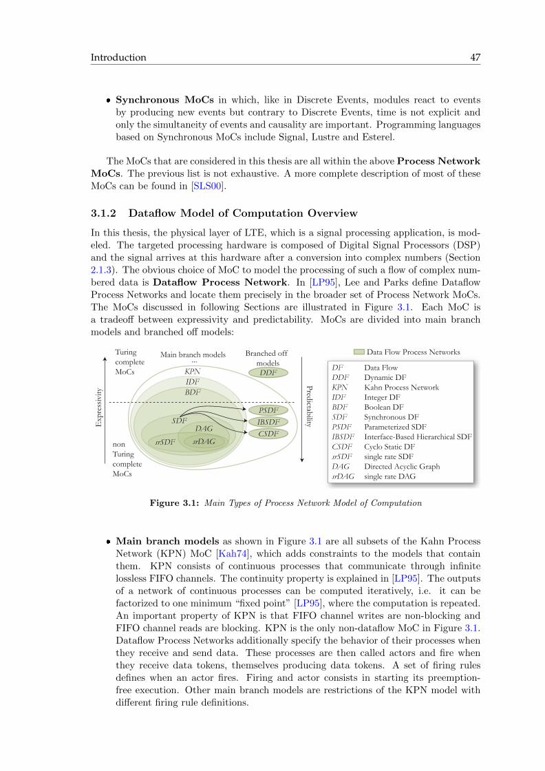
Introduction 47
� Synchronous MoCs in which, like in Discrete Events, modules react to eventsby producing new events but contrary to Discrete Events, time is not explicit andonly the simultaneity of events and causality are important. Programming languagesbased on Synchronous MoCs include Signal, Lustre and Esterel.
The MoCs that are considered in this thesis are all within the above Process NetworkMoCs. The previous list is not exhaustive. A more complete description of most of theseMoCs can be found in [SLS00].
3.1.2 Dataflow Model of Computation Overview
In this thesis, the physical layer of LTE, which is a signal processing application, is mod-eled. The targeted processing hardware is composed of Digital Signal Processors (DSP)and the signal arrives at this hardware after a conversion into complex numbers (Section2.1.3). The obvious choice of MoC to model the processing of such a flow of complex num-bered data is Dataflow Process Network. In [LP95], Lee and Parks define DataflowProcess Networks and locate them precisely in the broader set of Process Network MoCs.The MoCs discussed in following Sections are illustrated in Figure 3.1. Each MoC isa tradeoff between expressivity and predictability. MoCs are divided into main branchmodels and branched off models:
KPNIDFBDF
PSDF
CSDFSDF
DAG
srSDF srDAG
...
Exp
ress
ivity
Predictability
Turing complete MoCs
non Turing complete MoCs
DFDDFKPNIDFBDFSDFPSDFIBSDF CSDFsrSDF DAG srDAG
Data FlowDynamic DFKahn Process NetworkInteger DFBoolean DFSynchronous DFParameterized SDFInterface-Based Hierarchical SDFCyclo Static DFsingle rate SDFDirected Acyclic Graphsingle rate DAG
DDF
Main branch models Branched off models
Data Flow Process Networks
IBSDF
Figure 3.1: Main Types of Process Network Model of Computation
� Main branch models as shown in Figure 3.1 are all subsets of the Kahn ProcessNetwork (KPN) MoC [Kah74], which adds constraints to the models that containthem. KPN consists of continuous processes that communicate through infinitelossless FIFO channels. The continuity property is explained in [LP95]. The outputsof a network of continuous processes can be computed iteratively, i.e. it can befactorized to one minimum “fixed point” [LP95], where the computation is repeated.An important property of KPN is that FIFO channel writes are non-blocking andFIFO channel reads are blocking. KPN is the only non-dataflow MoC in Figure 3.1.Dataflow Process Networks additionally specify the behavior of their processes whenthey receive and send data. These processes are then called actors and fire whenthey receive data tokens, themselves producing data tokens. A set of firing rulesdefines when an actor fires. Firing and actor consists in starting its preemption-free execution. Other main branch models are restrictions of the KPN model withdifferent firing rule definitions.

48 Dataflow Model of Computation
� Branched off models are derived from main branch models with added featuresadapting their targeted usage to a particular problem, meaning that these modelsare no longer subsets of higher-level main branch MoCs.
When a given MoC is Turing complete, this MoC expresses all possible algorithms.Figure 3.1 distinguishes Turing complete MoCs from those that are non-Turing complete.The non-Turing complete MoCs have limited expressiveness but they enable more accuratecompile-time studies. Many Dataflow Process Network MoCs have been introduced in theliterature, each offering a tradeoff between compile-time predictability and capacity tomodel dynamic run-time variability. They differ mostly by their firing rules:
� Dynamic Data Flow MoC (DDF) is a MoC with special firing rules and is thusa dataflow process network MoC; but a DDF actor can “peek” at a token withoutconsuming it, thus defining non blocking reads not allowed in KPN. This propertycan make DDF non deterministic and complicate its study [LP95].Compared withKPN, DDF has advantages as a dataflow model. Contrary to the KPN processes,DDF actors do not necessitate a multi-tasking OS to be executed in parallel. Asimple scheduler that decides which actor to execute depending on the availabletokens is sufficient. The CAL language software execution method is based on thisproperty [JMRW10].
� The Synchronous Dataflow MoC (SDF) has been the most widely used dataflowMoC because of its simplicity and predictability. Each SDF actor consumes andproduces a fixed number of tokens at each firing. However, it is not Turing completeand cannot express conditions in an algorithm. Figure 3.2(a) shows a SDF algorithm.The small dots represent tokens already present on the edges when the computationstarts.
� The single rate SDF MoC is a subset of SDF. A single rate SDF graph is a SDFgraph where the production and consumption of tokens on an edge are always equal(Figure 3.2(b)).
� The Directed Acyclic Graph MoC (DAG) is also a subset of SDF. A DAG is aSDF graph where no path can contain an actor more than once, i.e. a graph thatcontains no cycle (Figure 3.2(c)).
� The single rate Directed Acyclic Graph MoC is a DAG where productions andconsumptions are equal.
� The Boolean Dataflow MoC (BDF) is a SDF with additional special actors calledswitch and select (Figure 3.2(d)). The switch actor is equivalent to a demultiplexerand the select actor to a multiplexer. The data tokens on the unique input of aswitch are produced on its true (respectively false) output if a control token evaluatedto true (respectively false) is sent to its control input. The BDF model adds controlflow to the SDF dataflow and it is this control that makes the model Turing complete.
� The Integer Data Flow MoC (IDF) is the equivalent of BDF but where the controltokens are integer tokens rather than Boolean tokens.
� The Cyclo Static Dataflow MoC (CSDF) extends SDF by defining fixed patternsof production and consumption (Figure 3.2(e)). For instance, a production patternof (1,2) means that the actor produces alternatively one and two tokens when it fires.

Introduction 49
� The Parameterized SDF MoC (PSDF) is a hierarchical extension of SDF thatdefines production and consumption relative to parameters that are reevaluated atreconfiguration points. Parameterized dataflow is a meta-modeling technique addingreconfigurability to a static model.
� The Interface-Based Hierarchical SDF MoC (IBSDF) is also a hierarchicalextension of SDF that insulates the behavior of its constituent graphs, making themeasy to combine and study. Interface-Based hierarchical dataflow is a meta-modelingtechnique which adds a hierarchy to a static model.
A B D
C
3 2 2 4
32 2
443
×12
(a) SDF
A B D
C
3 1
2 2
4×12
(b) single rate SDF
A B D
C
3 2 2 4
32 2
4
(c) DAG
switc
h
sele
ct
T
F
T
F
B
C
A D2
34
2
c
22
22
22
22
(d) BDF
A B D
C
3 (1,3) (3,1) 4
32 2
443
×12
(e) CSDF
Figure 3.2: A Few Dataflow MoC Graph Examples
The above list is not complete. Many more dataflow MoCs have been defined and newmodels are studied in this thesis in the context of the PREESM tool development. Dataflowprocess networks only specify how actors communicate but cannot give the complete ex-ecution semantics (for example, an actor performing an addition still needs a descriptionof this behavior to execute). If a Dataflow MoC is used for execution, it appears as acoordination language and must be combined with a host language defining actorbehavior [LP95]. C code can be used as a software host language or Hardware DescriptionLanguage (HDL) code as a hardware host language. CAL is a host language that cantarget both software and hardware implementation generation. In this study of LTE, Ccode is used as the host language but the code generation is flexible and may be adaptedto other programming languages.
Process networks are usually employed to model one execution of a repetitive process.For a single application, descriptions with different scales are often possible. When mod-eling an H.264 60 Hz full-HD video decoder for instance, a graph describing the decodingof one 16x16 pixels macro-block can be created and executed 486000 times per second. Itis also possible to create a graph describing the decoding of one picture and repeat thisdescription 60 times/s; or a graph describing the decoding of one group of pictures andwhich is then repeated several times per second. The right scale must be chosen, a scalewhich is too large produces graphs that are too large in terms of number of actors andcomplicates the study, whereas a scale that is too small will usually lead to sub-optimalimplementations [Nez02].
Aside from the scale, the granularity is another important parameter in describingan application. In [Sin07], Sinnen defines the granularity G of a system as the minimum

50 Dataflow Model of Computation
execution time of an actor divided by the maximum transfer time of an edge. Using thisdefinition which depends on both algorithm and architecture, in a coarse grain systemwhere G >> 1, actors are seen to be“costly” compared to the data flowing between them.High granularity is a desirable property for system descriptions because transfer timebetween operators does not add to the time efficiency of the system.
Because of different granularities and scales, there are several ways to describe a singleapplication. Choosing the correct MoC and using this model correctly is vital to obtainefficient prototyping results. In following sections, SDF, CSDF, and hierarchical extensionsof SDF are presented in more detail. The general theory of dataflow process networks canbe found in [LP95]. This thesis concentrates on the models used in the study of LTEphysical layer algorithms: SDF and its extensions.
3.2 Synchronous Data Flow
The Synchronous Dataflow (SDF) [LM87] is used to represent the behavior of an appli-cation at a coarse grain. An example of SDF graph is shown in Figure 3.2(a). SDF canmodel loops but not code behavioral modifications due to the nature of its input data.For example, an “if” statement cannot be represented in SDF.
The SDF model can be represented as a finite directed, weighted graph characterizedby the graph G =< V,E, d, p, c > where :
� V is the set of nodes; each node represents an actor that performs computation onone or more input data streams and produces one or more output data streams.
� E ⊆ V × V is the edge set, representing channels which carry data streams.
� d : E → N is the delay function with d(e) the number of initial tokens on an edge e(represented by black dots on the graph).
� p : E → N∗ is the production function with p(e) representing the number of datatokens produced by the e source actor at each firing and carried by e.
� c : E → N∗ is the consumption function with c(e) representing the number of datatokens consumed from e by the e sink actor at each firing.
This graph is a coordination language, and so only specifies the topology of thenetwork but does not give any information about the internal behavior of actors. Theonly behavioral information in the model is the amount of produced and consumed tokens.If only a simulation of the graph execution is needed, the actor behavior can usuallybe ignored and a few parameters like Deterministic Actor Execution Time (DAET) arenecessary. However, if the model will be used to generate executable code, a host codemust be associated with each actor.
3.2.1 SDF Schedulability
From a connected SDF representation, it should be possible to extract a valid single-coreschedule as a finite sequence of actor firings. The schedulability property of the SDF isvital; this enables the creation of a valid multi-core schedule. A valid schedule can firewith no deadlock and its initial state is equal to its final state.
A SDF graph can be characterized by a matrix close to the incidence matrix in graphtheory and called topology matrix. The topology matrix Γ is a matrix of size |E| × |V |,
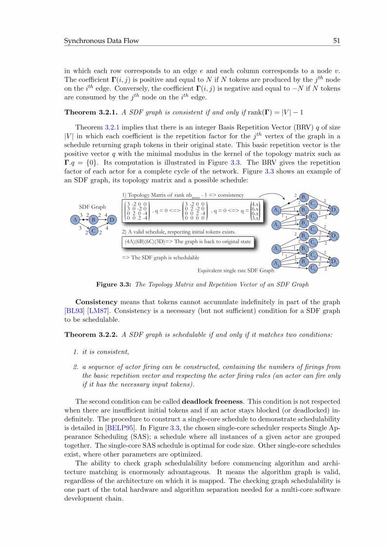
Synchronous Data Flow 51
in which each row corresponds to an edge e and each column corresponds to a node v.The coefficient Γ(i, j) is positive and equal to N if N tokens are produced by the jth nodeon the ith edge. Conversely, the coefficient Γ(i, j) is negative and equal to −N if N tokensare consumed by the jth node on the ith edge.
Theorem 3.2.1. A SDF graph is consistent if and only if rank(Γ) = |V | − 1
Theorem 3.2.1 implies that there is an integer Basis Repetition Vector (BRV) q of size|V | in which each coefficient is the repetition factor for the jth vertex of the graph in aschedule returning graph tokens in their original state. This basic repetition vector is thepositive vector q with the minimal modulus in the kernel of the topology matrix such asΓ.q = {0}. Its computation is illustrated in Figure 3.3. The BRV gives the repetitionfactor of each actor for a complete cycle of the network. Figure 3.3 shows an example ofan SDF graph, its topology matrix and a possible schedule:
A B D
C
3 2 2 4
32 2
4
3 -2 0 03 0 -2 00 2 0 -40 0 2 -4
. q = 0 <=>3 -2 0 00 2 -2 00 0 2 -40 0 0 0
. q = 0 <=> q = 4.x6.x6.x3.x
A1 B2 D1C2
B1C1
B3C3
A2
A3 B5C5
B4C4
B6C6
A4
D2
D3
1) Topology Matrix of rank nbactors - 1 => consistency
2) A valid schedule, respecting initial tokens exists.
(4A)(6B)(6C)(3D)=> The graph is back to original state
SDF Graph
Equivalent single rate SDF Graph
=> The SDF graph is schedulable
2
21
1 1 1
22
2
21
1 1 1
22
222
2
222
2
222
2
Figure 3.3: The Topology Matrix and Repetition Vector of an SDF Graph
Consistency means that tokens cannot accumulate indefinitely in part of the graph[BL93] [LM87]. Consistency is a necessary (but not sufficient) condition for a SDF graphto be schedulable.
Theorem 3.2.2. A SDF graph is schedulable if and only if it matches two conditions:
1. it is consistent,
2. a sequence of actor firing can be constructed, containing the numbers of firings fromthe basic repetition vector and respecting the actor firing rules (an actor can fire onlyif it has the necessary input tokens).
The second condition can be called deadlock freeness. This condition is not respectedwhen there are insufficient initial tokens and if an actor stays blocked (or deadlocked) in-definitely. The procedure to construct a single-core schedule to demonstrate schedulabilityis detailed in [BELP95]. In Figure 3.3, the chosen single-core scheduler respects Single Ap-pearance Scheduling (SAS); a schedule where all instances of a given actor are groupedtogether. The single-core SAS schedule is optimal for code size. Other single-core schedulesexist, where other parameters are optimized.
The ability to check graph schedulability before commencing algorithm and archi-tecture matching is enormously advantageous. It means the algorithm graph is valid,regardless of the architecture on which it is mapped. The checking graph schedulability isone part of the total hardware and algorithm separation needed for a multi-core softwaredevelopment chain.
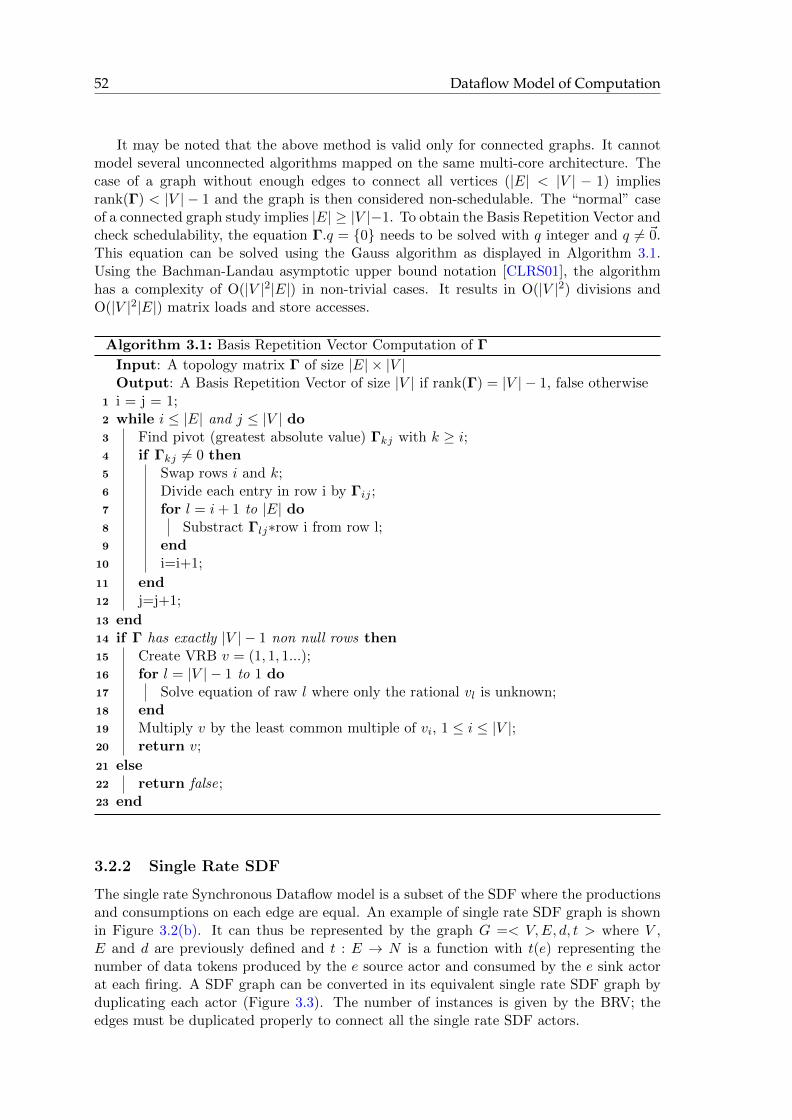
52 Dataflow Model of Computation
It may be noted that the above method is valid only for connected graphs. It cannotmodel several unconnected algorithms mapped on the same multi-core architecture. Thecase of a graph without enough edges to connect all vertices (|E| < |V | − 1) impliesrank(Γ) < |V | − 1 and the graph is then considered non-schedulable. The “normal” caseof a connected graph study implies |E| ≥ |V |−1. To obtain the Basis Repetition Vector andcheck schedulability, the equation Γ.q = {0} needs to be solved with q integer and q 6= ~0.This equation can be solved using the Gauss algorithm as displayed in Algorithm 3.1.Using the Bachman-Landau asymptotic upper bound notation [CLRS01], the algorithmhas a complexity of O(|V |2|E|) in non-trivial cases. It results in O(|V |2) divisions andO(|V |2|E|) matrix loads and store accesses.
Algorithm 3.1: Basis Repetition Vector Computation of Γ
Input: A topology matrix Γ of size |E| × |V |Output: A Basis Repetition Vector of size |V | if rank(Γ) = |V | − 1, false otherwise
1 i = j = 1;2 while i ≤ |E| and j ≤ |V | do3 Find pivot (greatest absolute value) Γkj with k ≥ i;4 if Γkj 6= 0 then5 Swap rows i and k;6 Divide each entry in row i by Γij ;7 for l = i+ 1 to |E| do8 Substract Γlj∗row i from row l;9 end
10 i=i+1;
11 end12 j=j+1;
13 end14 if Γ has exactly |V | − 1 non null rows then15 Create VRB v = (1, 1, 1...);16 for l = |V | − 1 to 1 do17 Solve equation of raw l where only the rational vl is unknown;18 end19 Multiply v by the least common multiple of vi, 1 ≤ i ≤ |V |;20 return v;
21 else22 return false;23 end
3.2.2 Single Rate SDF
The single rate Synchronous Dataflow model is a subset of the SDF where the productionsand consumptions on each edge are equal. An example of single rate SDF graph is shownin Figure 3.2(b). It can thus be represented by the graph G =< V,E, d, t > where V ,E and d are previously defined and t : E → N is a function with t(e) representing thenumber of data tokens produced by the e source actor and consumed by the e sink actorat each firing. A SDF graph can be converted in its equivalent single rate SDF graph byduplicating each actor (Figure 3.3). The number of instances is given by the BRV; theedges must be duplicated properly to connect all the single rate SDF actors.

Cyclo Static Data Flow 53
An algorithm to convert a SDF graph to a single rate SDF graph is given in [SB09]p. 45. It consists of successively adding actors and edges in the single rate SDF graphand has a complexity O(|V | + |E|) where V and E are the vertex set and the edge setrespectively of the single rate SDF graph.
3.2.3 Conversion to a Directed Acyclic Graph
One common way to schedule SDF graphs onto multiple processors is to first convert theSDF graph into a precedence graph so that each vertex in the precedence graph correspondsto a single actor firing from the SDF graph. Thus each SDF graph actor A is “expandedinto” qA separate precedence graph vertices, where qA is the component of the BRV thatcorresponds to A. In general, the precedence graph reveals more functional parallelism aswell as data parallelism. A valid precedence graph contains no cycle and is called DAG(Directed Acyclic Graph) or Acyclic Precedence Expansion Graph (APEG). In a DAG, anactor without input edge is called entry actor and an actor without output edge is calledexit actor. Unfortunately, the graph expansion due to the repeatedly counting each SDFnode can lead to an exponential growth of nodes in the DAG. Thus, precedence-graph-based multi-core scheduling techniques, such as the ones developed in [Kwo97], generallyhave a complexity that is not bounded polynomially in the input SDF graph size, and canresult in prohibitively long scheduling times for certain kinds of graphs [PBL95].
A B D
C
3 2 2 4
32 2
4BRV q =
4.x6.x6.x3.x
Valid schedule: (3A)(4B)(2D)(4C)A(2B)D(2C)
SDF Graphwith a cycle
Equivalent APEG
=> The SDF graph is schedulable
A1
A2
A3
A4
B2
B1
B3
B5
B4
B6
D1
D2
D3
C2
C1
C2
C1
C2
C1
21
1
2
2
11
2
2
2
2
2
2
2
2
2
2
2
2
2
Figure 3.4: SDF Graph and its Acyclic Precedence Expansion Graph
Converting a single rate SDF graph into its corresponding DAG simply consists ofignoring edges with initial tokens. If the graph is schedulable, each of its cyclic paths willcontain at least one initial token. Removing edges with initial tokens naturally breaksthese cycles and creates a DAG. Using this precedence graph as the algorithmic input forscheduling results in inter-iteration dependencies not being taken into account. Convertinga non-single rate SDF graph into its corresponding DAG is also possible but is a morecomplex operation as cycles must be unrolled before ignoring edges with initial tokens[Pia10].
3.3 Cyclo Static Data Flow
The Cyclo Static Dataflow (CSDF) model is introduced in [BELP95] and an examplegraph is shown in Figure 3.2(e). The CSDF model cannot express more algorithms thanSDF but it can express certain algorithms in a reduced way. CSDF can also enhanceparallelism and reduce memory necessary for execution. CSDF is used in the study ofLTE uplink and downlink streams. The token production and consumption of each actorcan vary over time, following a periodic form statically chosen. For example, an actor canconsume one token, then two tokens, then one token again, and so on. In this example,

54 Dataflow Model of Computation
the actor has two phases. In CSDF, token productions and consumptions are patternsinstead of scalars. A SDF model can be represented as a finite directed, weighted graphcharacterized by the graph G =< V,E, d, φ, p, c > where :
� V is the set of nodes; each node representing an actor.
� E ⊆ V × V is the edge set, representing data channels.
� d : E → N is the delay function with d(e) the number of initial tokens on an edge e.
� φ : V → N) is the phase function with φ(v) the number of phases in the patternexecution of v.
� p : E × N→ N∗ is the production function with p(e, i) representing the number ofdata tokens produced by the e source actor at each firing of phase i and carried bye.
� c : E × N → N∗ is the consumption function with c(e, i) representing the numberof data tokens consumed from e by the e sink actor at each firing of phase i.
The CSDF model introduces the notion of actor state; an actor does not behave thesame at each firing. However, the fixed pattern of execution permits to check the graphschedulability at compile-time.
3.3.1 CSDF Schedulability
Like a SDF graph, a CSDF graph can be characterized by its topology matrix. Thetopology matrix Γ is the matrix of size |E|× |V |, where each row corresponds to an edge eand each column corresponds to a node v. The coefficient Γ(i, j) is positive and equal to∑φ(j)
k=1 p(i, k) if a pattern p(i, k) is produced by the jth node on the ith edge. Conversely, the
coefficient Γ(i, j) is negative and equal to −∑φ(j)
k=1 c(i, k) if a pattern c(i, k) is consumedby the jth node on the ith edge.
The topology matrix gathers the cumulative productions and consumptions of eachactor during its complete period of execution. A CSDF graph G is consistent if and onlyif the rank of its topology matrix Γ is one less than the number of nodes in G (Theorem3.2.1). However, the smallest vector q′ in Γ null space is not the BRV. q′ only reflects thenumber of repetitions of each complete actor cycle and must be multiplied for each actorv by its number of phases φ(v) to obtain the BRV q:
q = Φ× q′, with Φ = diag(φ(v1), φ(v2), . . . , φ(vm)) (3.1)
A valid sequence of firings with repetitions given by the BRV is still needed to concludethe schedulability of the graph. The process is illustrated in Figure 3.5. It can be concludedon CSDF schedulability as in the SDF case. Figure 3.6 illustrates a compact representationof a CSDF graph and its SDF equivalent. In this simple example, the number of verticeshas been reduced by a factor 2.3 by using CSDF instead of SDF.
3.4 Dataflow Hierarchical Extensions
A hierarchical dataflow model contains hierarchical actors. Each hierarchical actor con-tains a net of actors. There are several ways to define SDF actor hierarchy. The first SDF

Dataflow Hierarchical Extensions 55
A B D
C
3(1,3) (3,1)
4
32 2
4
3 -4 0 03 0 -2 00 4 0 -40 0 2 -4
. q' = 0 <=>3 -4 0 00 4 -2 00 0 2 -40 0 0 0
. q' = 0 <=> q' = 4.x3.x6.x3.x
A1 B2 D1C2
B1C1
B3C3
A2
A3 B5C5
B4C4
B6C6
A4
D2
D3
1) Topology Matrix of rank nbactors - 1 => consistency
2) A valid schedule, respecting initial tokens exists.
(4A)(6B)(6C)(3D)=> The graph is back to original state
CSDF Graph
Equivalent single rate SDF Graph=> The CSDF graph is schedulable
12
21 1 1
21
2 21
1 1
23
321
2
321
2
321
2
q = q' .1 0 0 00 2 0 00 0 1 00 0 0 1
= 4.x6.x6.x3.x
1Multiplying by the number of phases of each actor
Figure 3.5: The Topology Matrix and Repetition Vector of a CSDF Graph
A B6 (1,2,3) 2
C(3,2,1)
A B1
C
B
B
23
1
2
3
C
C
1
1
2 2
1
111
1
1
CSDF SDF
Figure 3.6: Illustrating Compactness of CSDF Model Compared to SDF
hierarchy was that of clustering described in [PBL95] by Pino, et al. The study takes abottom-up approach and defines rules that extract the actors from a complex graph whichcan be clustered within a coarser-grain actor. The primary advantage of this techniqueis that clustered actors are then easier than the individual actors in scheduling processmanipulations.
However, the type of hierarchy that is of interest in this thesis is a top-down one: aSDF hierarchy that allows a designer to compose sub-graphs within an upper-level graph.Two such hierarchy models have been defined and both will be studied in this thesis: theParameterized SDF (PSDF [BB01]) and the Interface-Based Hierarchical SDF (IBSDF[PBPR09]).
3.4.1 Parameterized Dataflow Modeling
Parameterized dataflow modeling is a technique that can be applied to all dataflow modelswith deterministic token rates, in particular to SDF and CSDF [BB02]. It consists ofcreating a hierarchical view of the algorithm whose subsystems are then composed of 3graphs:
� the body graph φb: this is the effective dataflow sub-graph. Its productions andconsumptions depend on certain parameters. These parameters are called topologyparameters because they affect the topology of the body graph. The behavior of theactors (not expressed in the coordination language) depends on parameters that willbe called actor parameters.
� the init graph φi: this graph is launched one time only when a subsystem interfaceis reached, i.e. once per invocation of the subsystem. It performs a reconfigurationof the subsystem, setting parameters that will be common to all φb firings duringthe invocation. φi does not consume any data token.
� the subInit graph φs: it is launched one time before each body graph firing and alsosets parameters. φs can consume data tokens.
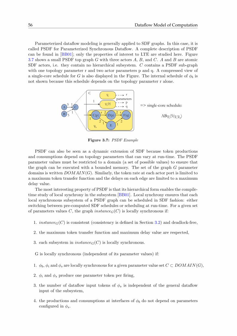
56 Dataflow Model of Computation
Parameterized dataflow modeling is generally applied to SDF graphs. In this case, it iscalled PSDF for Parameterized Synchronous Dataflow. A complete description of PSDFcan be found in [BB01]; only the properties of interest to LTE are studied here. Figure3.7 shows a small PSDF top graph G with three actors A, B, and C. A and B are atomicSDF actors, i.e. they contain no hierarchical subsystem. C contains a PSDF sub-graphwith one topology parameter r and two actor parameters p and q. A compressed view ofa single-core schedule for G is also displayed in the Figure. The internal schedule of φb isnot shown because this schedule depends on the topology parameter r alone.
φs(r)
φi r
q1
C(p)r 2
D(p)
E
F(q)2 r
2 1 21
p
1
φb
A C
B
5 1
51
C
parameters
=> single-core schedule:
ABφi(5(φsφb)
Figure 3.7: PSDF Example
PSDF can also be seen as a dynamic extension of SDF because token productionsand consumptions depend on topology parameters that can vary at run-time. The PSDFparameter values must be restricted to a domain (a set of possible values) to ensure thatthe graph can be executed with a bounded memory. The set of the graph G parameterdomains is written DOMAIN(G). Similarly, the token rate at each actor port is limited toa maximum token transfer function and the delays on each edge are limited to a maximumdelay value.
The most interesting property of PSDF is that its hierarchical form enables the compile-time study of local synchrony
¯in the subsystem [BB01]. Local synchrony ensures that each
local synchronous subsystem of a PSDF graph can be scheduled in SDF fashion: eitherswitching between pre-computed SDF schedules or scheduling at run-time. For a given setof parameters values C, the graph instanceG(C) is locally synchronous if:
1. instanceG(C) is consistent (consistency is defined in Section 3.2) and deadlock-free,
2. the maximum token transfer function and maximum delay value are respected,
3. each subsystem in instanceG(C) is locally synchronous.
G is locally synchronous (independent of its parameter values) if:
1. φb, φi and φs are locally synchronous for a given parameter value set C ⊂ DOMAIN(G),
2. φi and φs produce one parameter token per firing,
3. the number of dataflow input tokens of φs is independent of the general dataflowinput of the subsystem,
4. the productions and consumptions at interfaces of φb do not depend on parametersconfigured in φs.

Dataflow Hierarchical Extensions 57
If G is locally synchronous, a local SDF schedule can be computed at run-time toexecute the graph. Though φi and φs can set both topology and actor parameters, generalpractice is for φs to only change actor parameters so identical firings of φb occur for eachsubsystem invocation. When this condition is satisfied, a local SDF schedule only needsto be computed once after φi is executed. Otherwise, the local SDF schedule needs to becomputed after each φs firing.
In this LTE study, Parameterized CSDF is also of interest; this is equivalent to PSDFexcept the parameters are not only scalars but can be patterns of scalars similar to theCSDF model. For this thesis, the PDSF init and the PSDF sub-init graphs employed aredegenerated graphs containing only a single actor and do not consume or produce any datatokens. They are thus represented by a simple rectangle illustrating the actor execution(Chapter 8).
3.4.2 Interface-Based Hierarchical Dataflow
Interface-Based Hierarchical Dataflow Modeling is introduced by Piat, et al. in [PBR09]and [PBPR09]. Like Parameterized Dataflow Modeling, it may be seen as a meta-modelthat can be applied to several deterministic models. The objective of Interface-BasedHierarchical Dataflow Modeling is to allow a high-level dataflow graph description of anapplication, composed of sub-graphs. If an interface is not created to insulate the uppergraph from its sub-graphs, the actor repetitions of sub-graphs can result in the actorrepetitions of the upper graph appearing illogical to the programmer. The Interface-Based Hierarchical Dataflow Modeling has been described in combination with SDF in theso-called Interface-Based Hierarchical SDF or IBSDF. The model obtained encapsulatessub-graphs and protects upper graphs. Encapsulation is a very important model property;it enables the combination of semiconductor intellectual property cores (commonly calledIPs) in electronic design and is the foundation of object oriented software programming.
The operation of hierarchy flattening consists of including a sub-graph within its par-ent graph while maintaining the general system behavior. Figure 3.8(a) shows an exampleof a SDF graph with a hierarchical actor of which the programmer will probably wantthe sub-graph to be repeated three times. Yet, the sub-graph behavior results in a verydifferent flattened graph, repeating the actor A from the upper graph. Figure 3.8(b) illus-trates the same example described in as a IBSDF graph. Source and sink interfaces havebeen introduced. The resulting flattened graph shape is more intuitive. The additionalbroadcast actors have a circular buffering behavior: as each input is smaller in size thanthe sum of their outputs, they duplicate each input token in their output edges.
A B C3 1 1 3
D E1 2 11
CEE
E
DD
D
DD
D
AA
(a) Hierarchical SDF Example Flattening
A B C3 1 1 3
D E1 2 11
CEE
E
DD
D
DD
D
src snk
b
b
b
A
1
1
1
11
11
11
(b) IBSDF Example Graph Flattening
Figure 3.8: Comparing Direct Hierarchical SDF with IBSDF
Compared with other SDF actors, the IBSDF interfaces have specific behavior. Theyare designed to constitute code closures (i.e. semantic boundaries). The IBSDF type of

58 Dataflow Model of Computation
hierarchy is closer to host language semantics such as C, Java and Verilog. The additionalfeatures have been shown to introduce no deadlock [PBPR09].
A Source node is a bounded source of tokens which represents the tokens available fora sub-graph iteration. This node acts as an interface to the outside world. A source portis defined by the four following rules:
1. Source production homogeneity: A source node Source produces the sameamount of tokens on all its outgoing connections p(e) = n ∀e ∈ {Source(e) =Source}.
2. Interface Scope: The source node remains write-locked during an iteration of thesub-graph. This means that the interface cannot be externally filled during thesub-graph execution.
3. Interface boundedness: A source node cannot be repeated, thus any node con-suming more tokens than available from the node will consume the same tokensmultiple times (i.e. circular buffer). c(e)%p(e) = 0 ∀e ∈ {source(e) = source}.
4. SDF consistency: All the tokens available from a source node must be consumedduring an iteration of the sub-graph.
A sink node is a bounded sink of tokens that represent the tokens to be produced byone iteration of the sub-graph. This node behaves as an external interface. A sink nodeis defined by the four following rules:
1. Sink producer uniqueness: A sink node Sink only has one incoming connection.
2. Interface Scope: The sink node remains read-locked during an iteration of the sub-graph. This means that the interface cannot be externally read during the sub-graphexecution.
3. Interface boundedness: A sink node cannot be repeated, thus any node producingmore tokens than needed will write the same tokens multiple times (i.e. ring buffer).p(e)%c(e) = 0 ∀e ∈ {target(e) = Sink}.
4. SDF consistency: All tokens consumed by a sink node must be produced duringan iteration of the sub-graph.
A B3 1 1
snk1
A
B11
1
snk
B2
B3
111
11 1
1
Figure 3.9: IBSDF Sub-Graph Example and Its Single Rate Equivalent
Source and sink nodes cannot be repeated, providing a fixed reference interface tocombine these nodes in an upper level graph. A source node, behaving as a circularbuffer, sends the same tokens to its graph possibly several times. A sink node, behavingas a circular buffer, stores the last tokens received from its graph. Figure 3.9 shows anexample of an IBSDF graph and its single rate equivalent. IBSDF has an extremelyimportant property: an IBSDF graph is schedulable if and only if its constituent SDF

Dataflow Hierarchical Extensions 59
sub-graphs are schedulable [PBR09]. Moreover, the interfaces do not influence SDF sub-graph schedulability. Independently applying the SDF BRV calculation to each algorithmpart with complexity O(|V |2|E|) presented in Section 3.2 makes the overall calculationmuch faster.
In this thesis, IBSDF is the model chosen to describe LTE algorithms for rapid proto-typing. Several features have been added for the use of IBSDF in PREESM to enhanceexpressivity and ease code generation. The final model is presented in section 6.2.1.
While chapters 2 and 3 introduced the target application of this study and the MoCsavailable to model it, chapter 4 will detail the process of rapid prototyping, which will beapplied to LTE in the following chapters.

60 Dataflow Model of Computation

CHAPTER 4
Rapid Prototyping and Programming Multi-core Architectures
4.1 Introduction
This chapter gives an over view of the existing work on rapid prototyping and multi-coredeployment in the signal processing world. The concept of rapid prototyping was intro-duced in Figure 1.2 when outlining the structure of this thesis. It consists of automaticallygenerating a system simulation or a system prototype from quickly constructed models.Rapid prototyping may be used for several purposes; this study uses it to manage the par-allelism of DSP architectures. Parallelism must be handled differently for the macroscopicor microscopic views of a system. The notions that are developed in this section will beused to study LTE in Part II. Section 4.2 gives an insight into embedded heterogeneousarchitectures. Section 4.3 is an overview of the multi-core programming techniques andSection 4.4 focuses on the internal mechanism of multi-core scheduling. Finally, Section4.5 presents some results from the literature on automatic code generation.
4.1.1 The Middle-Grain Parallelism Level
The rapid prototyping and programming method focuses on particular classes of algorithmsand architecture, and a certain degree of parallelism. This study targets signal processingapplications running on multi-core heterogeneous systems and the objective is to exploittheir middle-grain parallelism. These terms are defined in next sections.
The problem of parallel execution is complex and analysis is aided if it is brokendown into sub-problems. An application does not behave similarly at system-level or low-level. Three levels of granularity are usually evoked in literature and concurrency canbe exploited at each of these three levels: Instruction-Level Parallelism (ILP), Thread-Level Parallelism (ThLP) and Task-Level Parallelism (TLP). An instruction is a singleoperation of a processor defined by its Instruction Set Architecture (ISA). The term taskis used here in the general sense of program parts that share no or little information witheach other. Tasks can contain several threads that can run concurrently but have dataor control dependencies. The three levels of granularity are used to specify parallelism ina hierarchical way. Table 4.1 illustrates the current practices in parallelism extraction ofapplications.
The Task Level Parallelism concerns loosely coupled processes with few depen-
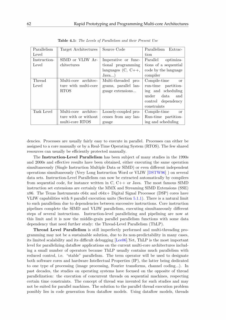
62 Rapid Prototyping and Programming Multi-core Architectures
Table 4.1: The Levels of Parallelism and their Present Use
ParallelismLevel
Target Architectures Source Code Parallelism Extrac-tion
Instruction-Level
SIMD or VLIW Ar-chitectures
Imperative or func-tional programminglanguages (C, C++,Java...)
Parallel optimiza-tions of a sequentialcode by the languagecompiler
ThreadLevel
Multi-core architec-ture with multi-coreRTOS
Multi-threaded pro-grams, parallel lan-guage extensions...
Compile-time orrun-time partition-ing and schedulingunder data andcontrol dependencyconstraints
Task Level Multi-core architec-ture with or withoutmulti-core RTOS
Loosely-coupled pro-cesses from any lan-guage
Compile-time orRun-time partition-ing and scheduling
dencies. Processes are usually fairly easy to execute in parallel. Processes can either beassigned to a core manually or by a Real-Time Operating System (RTOS). The few sharedresources can usually be efficiently protected manually.
The Instruction-Level Parallelism has been subject of many studies in the 1990sand 2000s and effective results have been obtained, either executing the same operationsimultaneously (Single Instruction Multiple Data or SIMD) or even different independentoperations simultaneously (Very Long Instruction Word or VLIW [DSTW96] ) on severaldata sets. Instruction-Level Parallelism can now be extracted automatically by compilersfrom sequential code, for instance written in C, C++ or Java. The most famous SIMDinstruction set extensions are certainly the MMX and Streaming SIMD Extensions (SSE)x86. The Texas Instruments c64x and c64x+ Digital Signal Processor (DSP) cores haveVLIW capabilities with 8 parallel execution units (Section 5.1.1). There is a natural limitto such parallelism due to dependencies between successive instructions. Core instructionpipelines complete the SIMD and VLIW parallelism, executing simultaneously differentsteps of several instructions. Instruction-level parallelizing and pipelining are now atthis limit and it is now the middle-grain parallel parallelism functions with some datadependency that need further study: the Thread-Level Parallelism (ThLP).
Thread Level Parallelism is still imperfectly performed and multi-threading pro-gramming may not be a sustainable solution, due to its non-predictability in many cases,its limited scalability and its difficult debugging [Lee06].Yet, ThLP is the most importantlevel for parallelizing dataflow applications on the current multi-core architectures includ-ing a small number of operators because ThLP usually contains much parallelism withreduced control, i.e. “stable” parallelism. The term operator will be used to designateboth software cores and hardware Intellectual Properties (IP), the latter being dedicatedto one type of processing (image processing, Fourier transforms, channel coding...). Inpast decades, the studies on operating systems have focused on the opposite of threadparallelization: the execution of concurrent threads on sequential machines, respectingcertain time constraints. The concept of thread was invented for such studies and maynot be suited for parallel machines. The solution to the parallel thread execution problempossibly lies in code generation from dataflow models. Using dataflow models, threads

Modeling Multi-Core Heterogeneous Architectures 63
are replaced by actors that have no side effects, are purely functional and communicatethrough well defined data channels [LP95]. A side effect is a modification of a thread stateby another thread due to shared memory modifications. Using actors, thread-Level paral-lelism then becomes Actor Level Parallelism (ALP); the general problem of managingparallelism at ThLP and ALP will be called middle-grain parallelism.
While task and instruction parallelism levels are already managed efficiently in prod-ucts, middle-grain parallelism level is still mostly at a research phase. The PREESMframework aims to provide a method for an efficient and automatic middle-grain paral-lelization.
4.2 Modeling Multi-Core Heterogeneous Architectures
4.2.1 Understanding Multi-Core Heterogeneous Real-Time EmbeddedDSP MPSoC
The target hardware architectures of this thesis are associated with a great number ofnames and adjectives. These terms need definitions:
� DSP can refer to both Digital Signal Processing and Digital Signal Processor. In thisthesis, DSP is used to refer to Digital Signal Processors, i.e. processors optimized toefficiently compute digital signal processing tasks.
� An embedded system is a calculator contained in a larger system embedded intothe environment it controls. Real-time embedded systems include mobile phones,multimedia set-top boxes, skyrocket and, of interest in this thesis, wireless commu-nication base stations. Only systems with very strict constraints on power consump-tion will be considered; this does not include hardware architectures consuming tensor hundreds of Watts such as Graphical Processing Units (GPU) or general purposeprocessors. The study concentrates on Digital Signal Processors (DSP), which arewell suited for real-time embedded signal processing systems.
� A real-time system must respect the time constraints defined by the runningapplication and produce output data at the exact time the environment requires it.Real-time systems include video or audio decoding for display, machine-tool control,and so on.
� Multi-Core is a generic term for any system with several processor cores able toconcurrently execute programs with Middle-grain or Task-Level Parallelism.
� Heterogeneous refers to the existence of different types of operators within thesystem. It can also refer to the non-symmetrical access to resources, media withdiffering performances or cores with different clock speeds.
� A Multi-Processor System-on-Chip or MPSoC is a term widely used to designatea multi-core system embedded in a single chip.
In general, modern multi-core embedded applications are manually programmed, us-ing C or C++ sequential code, and optimized using assembly code. Manual multi-coreprogramming is a complex, error-prone and slow activity. The International TechnologyRoadmap for Semiconductors (ITRS) evaluates that embedded software productivity dou-bles every five years; this is a much slower growth than that of processor capabilities.ITRS predicts the cost of embedded software will increase until 2012 where it will reach

64 Rapid Prototyping and Programming Multi-core Architectures
three times the total cost of embedded hardware development. At that time, parallel de-velopment tools are predicted to reduce software development costs drastically [fS09]. Thegoal of this study is to contribute to this evolution.
Today, Multi-core digital signal operators, including up to several DSPs, face a choice.They may choose to use a small number of complex cores or to use many simple ones.The more cores are involved, the more complex the problem of exploiting them correctlybecomes. With a few exceptions, the present trend in powerful digital signal process-ing architectures is to embed a small number of complex processor cores on one die[KAG+09]. Software-defined radio, where signal processing algorithms are expressed insoftware rather than in hardware, is now widely used for embedded systems includingbase stations. However, certain repetitive compute-hungry functionalities can make atotally software-defined system suboptimal. Hardware accelerators, also known as copro-cessors, can process compute-hungry functionalities in a power-efficient way. They costprogramming flexibility but increase the system power efficiency. The current work studiesheterogeneous multi-core and multi-processor architectures with a few (or a few tens) com-plex DSP cores associated with a small number of hardware coprocessors. Architectureswith more than a few tens of operators are (currently) called “many-core”.
In following sections, the term multi-core system is used for the very general case ofeither one processor with several cores or several interconnected processors. The nextsection explores architecture modeling for such systems.
4.2.2 Literature on Architecture Modeling
Today, processor cores are still based on the Von Neumann model created in 1946,as illustrated in Figure 4.1. It consists of a memory containing data and programs, anArithmetic and Logic Unit (ALU) that processes data, input and output units that com-municate externally, and a control unit that drives the ALU and manages the program.Externally, this micro-architecture can be seen as a black box implementing an Instruc-tion Set Architecture (ISA), writing/reading external memory and sending/receivingmessages. Such an entity is called an operator. An operator can have an ISA so restrictedthat it is no longer considered to a processor core but a coprocessor dedicated to one or afew tasks.
Control Unit
ALUInput Unit Output Unit
Memory Unit
Instruction Set ArchitectureVon NeumannArchitecture
Operator
Figure 4.1: The Von Neumann Architecture of an Operator
The literature on architecture models is less extensive than that of algorithm models.The majority of the literature focuses on classifying architectures, and associating specificarchitectures to categories. Processors have been split between Complex Instruction SetComputer (CISC) and Reduced Instruction Set Computer (RISC) depending on their in-struction set complexity [Hea95]. The limit between CISC and RISC machines is generallyunclear. Many instruction sets exist, each with its own tradeoff between core clock speedand advanced instruction capabilities. Tensilica [Ten] is a company known for tools capa-
Multi-core Programming 65
ble of generating DSP cores with customizable ISA. Thus, CISC or RISC may no longerbe a valid criterion to define a processor.
The Flynn taxonomy [Fly72] has introduced four categories of machines classified de-pending on their instruction and/or data parallelism at a given time: Single InstructionSingle Data (SISD), Single Instruction Multiple Data (SIMD), Multiple Instruction SingleData (MISD) and Multiple Instruction Multiple Data (MIMD). MIMD machines, requir-ing many control information at each clock cycle, have been implemented using Very LongInstruction Words (VLIW). MIMD systems have a sub-classification [BEPT00] based ontheir memory architecture types, splitting MIMD machines into 3 categories:
� A Uniform Memory Access (UMA) machine has a memory common to all itsoperators which is accessed at the same speed with the same reliability. This sharedmemory is likely to become the bottleneck of the architecture; two solutions canincrease the access speed: it may be divided into banks attributed to a specificoperator in a given time slot or it may be accessed via a hierarchical cache.
� A Non Uniform Memory Access (NUMA) machine has a memory common toall its operators but access speed to this memory is heterogeneous. Some operatorshave slower access speeds than others.
� A NO Remote Memory Access (NORMA) machine does not have a shared mem-ory. Operators must communicate via messages. NORMA architecture is usuallycalled distributed architecture because no centralized memory entity exists.
In Chapter 5, a new system-level architecture model is introduced. Architecture modelsexist in the literature but they were not suited to model target architectures for rapid pro-totyping. The SystemC language [sys] and its Transaction Level Modeling (TLM) is a setof C++ templates that offers an efficient standardized way to model hardware behavior.Its focus is primarily the study and debugging of the hardware and software function-alities before the hardware is available. It defines abstract modules that a programmercan customize to its needs. For this rapid prototyping study, more precise semantics ofarchitecture element behaviors are needed than those defined in SystemC TLM. Anotherexample of language targeting hardware simulation is a language created by the Societyof Automotive Engineers (SAE) and named Architecture Analysis and Design Language(AADL [FGHI06]). The architecture part of this language is limited to the three nodes:processor, memory and bus. Processes and threads can be mapped onto the processors.This model is not adaptable to the study presented here because it focuses on impera-tive software containing preemptive threads and the architecture nodes are insufficient tomodel the target architectures with Direct Memory Accesses (DMA) and switches (Section5.1.1).
In next section, existing work on multi-core programming is presented.
4.3 Multi-core Programming
4.3.1 Middle-Grain Parallelization Techniques
Middle-grain parallelization consists of four phases: extraction, assignment, orderingand timing. Parallel actors must be extracted from the source code or model and alltheir dependencies must be known. Parallel actors are then assigned (or mapped) tooperators available in the target architecture. Their execution on operators must also be

66 Rapid Prototyping and Programming Multi-core Architectures
Sources
Actor1 Actor2Actor3 Actor4
Core1 Core2
Actor1 Actor2Actor3 Actor4
Core1 Core2
Time
3 2
14
Core1 Core2
Actor1 Actor2Actor3 Actor4
21
12
Parallel Regions
Timing
Extraction
Assignm
ent
Ordering
Figure 4.2: The Four Phases of Middle-Grain Parallelization: Extraction, Assignment, Orderingand Timing
ordered (or scheduled) because usually, there are fewer operators than actors. Finally, astart time for the execution of each actor must be chosen. The four tasks of extraction,assignment, ordering and timing, are illustrated in Figure 4.2. Graham showed in the1960s that relaxing certain constraints in a parallel system with dependencies can leadto worsened performance when using a local mapping and scheduling approach [Gra66],making middle-grain parallelism extraction a particularly complex task.
In [POH09], Park, et al. divide the current embedded system design methods into4 categories based on their input algorithm description. All four methods focus on themiddle-grain parallelism level:
� Compiler-based design methods extract middle-grain parallel actors from sequen-tial code such as C-code, and map actors on different operators to enable their parallelexecution. The method is analogous to that broadly adopted for the Instruction-Level. The obvious advantage of this method is the automatic parallelization oflegacy code and, for an efficient compiler, no further effort is required from soft-ware engineers to translate their code. The key issue in the complex operation ofparallelism extraction is to find middle-grain actors, coarse-grained enough to groupdata transfers efficiently and fine-grained enough to enable high parallelism. Us-ing imperative and sequential code as an input, these methods are very unlikely toexploit all the algorithm potential parallelism. An example of a compiler implement-ing compiler-based method is the MPSoC Application Programming Studio (MAPS)from Aachen RWTH University [CCS+08] which generates multi-threaded C codefrom sequential C code and parallelizes these threads.
� Language-extension design methods consist of adding information to a sequen-tial language that eases parallel actors’ extraction. With Open Multiprocessing(OpenMP [opeb]) for instance, a programmer can annotate C, C++ or Fortrancode and indicate where he wants parallelism to be extracted. The CILK language[BJK+95] from the Massachusetts Institute of Technology is another example of sucha technology adapted to C++. The compiler automates the mapping and transfersof parallel actors. OpenMP is already supported by the majority of the C, C++ andFortran compilers. It was developed for Symmetric Multi-Processor (SMP) archi-tectures and is likely to offer sub-optimal solutions for heterogeneous architectures.Other language extensions for parallelism that exist are less automated: MessagePassing Interface (MPI), OpenCL [opea] or the Multicore Association API [mca]which offers APIs for manual multi-core message passing or buffer sharing.
� Platform-based methods actually refers to a single solution based on a CommonIntermediate Code (CIC) [KKJ+08], equivalent to a compiler Intermediate Repre-sentation (IR) with parallelism expressivity. It is intended to create an abstractionof the platform architecture to the compiler front-end that extracts parallelism.

Multi-core Programming 67
� Model of Computation (MoC)-based design methods describe high-level appli-cation behavior with simple models. While compilation-based parallelization appealsto programmers because they can almost seamlessly reuse their huge amount of ex-isting sequential code (generally in C or C++), MoC-based design methods bringseveral advantages compared with previous methods. They are aimed at expressinghigh-level algorithm descriptions into simple textual files or graph-based GraphicalUser Interfaces. MoC-based methods have three great advantages. Firstly, paral-lelism is naturally expressed by a graph. An extraction with a compilation algorithmwill always under-performing on certain cases. The first step of Figure 4.2 becomesstraightforward. Secondly, certain rules of a model-based design (such as schedu-lability) can be verified at compile-time and correct-by-construction high-level codemay be generated. Thirdly, the transaction-level form of dataflow graphs can en-able co-simulation of entities of different forms. This is why the Transaction-LevelModeling (TLM [Ghe06]) of SystemC is based on a dataflow MoC. Hardware-definedmodules can be interconnected with software-defined modules.
As explained in Chapter 3, dataflow MoCs have been chosen to represent algorithmsin the development of the rapid prototyping method and the prototyping frameworkPREESM.
4.3.2 PREESM Among Multi-core Programming Tools
There exist numerous solutions to partition algorithms onto multi-core architectures. Ifthe target architecture is homogeneous, several solutions will generate multi-core codefrom C with additional information (OpenMP [opeb], CILK [BJK+95]). In the case ofheterogeneous architectures, languages such as OpenCL [opea] and the Multicore Associ-ation Application Programming Interface (MCAPI [mca]) define ways to express parallelproperties of a code. However, they are not currently linked to efficient compilers andrun-time environments. Moreover, compilers for such languages would have difficulty inextracting and solving the bottlenecks inherent to graph descriptions of the architectureand the algorithm. A bottleneck is a feature limiting the system performance.
The Poly-Mapper tool from PolyCore Software [pol] offers functionalities similar toPREESM but, in contrast to PREESM, has manual mapping/scheduling. Ptolemy II[Lee01] is a simulation tool that supports many computational models. However, it has noautomatic mapping and its current code generation for embedded systems is focused onsingle-core targets. Another family of frameworks existing for dataflow based programmingis based on CAL [EJ03] language and it includes OpenDF [BBE+08]. OpenDF employsa more dynamic model than PREESM but its related code generation does not currentlysupport multi-core embedded systems.
Closer in principle to PREESM are the Model Integrated Computing (MIC [KSLB03]),the Open Tool Integration Environment (OTIE [Bel06]), the Synchronous DistributedExecutives (SynDEx [GLS99]), the Dataflow Interchange Format (DIF [HKK+04]), andSDF for Free (SDF3 [Stu07]). Both MIC and OTIE cannot be found on internet. Accordingto the literature, MIC focuses on the transformation between algorithm domain-specificmodels and meta-models while OTIE defines a single system description that can be usedduring the whole signal processing design cycle.
DIF is designed as an extensible repository of representation, analysis, transformationand scheduling of dataflow language. DIF is a Java library which allows the user to go fromgraph specification using the DIF language to C code generation. However, the IBSDFmodel (Section 3.4.2) as used in PREESM is not available in DIF.

68 Rapid Prototyping and Programming Multi-core Architectures
Table 4.2: Scheduling strategies
assignment ordering timing
fully dynamic run run run
static-assignment compile run run
self-timed compile compile run
fully static compile compile compile
SDF3 is an open source tool implementing certain dataflow models and providinganalysis, transformation, visualization, and manual scheduling as a C++ library. SDF3implements the Scenario Aware Dataflow (SADF [The07]), and provides a Multi-ProcessorSystem-on-Chip (MP-SoC) binding/scheduling algorithm to output as MP-SoC configu-ration files.
SynDEx and PREESM are both based on the AAM methodology [GS03] but thesetools do not possess the same features. SynDEx is not open source, has a unique Modelof Computation that does not support schedulability analysis and the function of codegeneration is possible but not provided with the tool. Moreover, the architecture modelof SynDEx is at too high a level to account for bus contentions and DMA used in modernchips (multi-core processors of MP-SoC) in mapping/scheduling.
The features that differentiate PREESM from the related works and similar tools are :
� The tool is open source and accessible online,
� The algorithm description is based on a single well-known and predictable model ofcomputation,
� The scheduling is totally automatic,
� The functional code for heterogeneous multi-core embedded systems can be generatedautomatically,
� The IBSDF algorithm model provides a helpful hierarchical encapsulation thus sim-plifying the scheduling [PBPR09].
The rapid prototyping method used in this study and the PREESM tool have a multi-core scheduler as the central feature. The multi-core scheduling techniques proposed in thisstudy are based on well-known algorithms from the literature presented in next section.
4.4 Multi-core Scheduling
4.4.1 Multi-core Scheduling Strategies
In [Lee89], Lee develops a taxonomy of scheduling algorithms that distinguishes run-timeand compile-time scheduling steps. The choice of the scheduling steps executed at compile-time and the ones executed at run-time is called a scheduling strategy. The taxonomy ofscheduling strategies is summarized in Table 4.2. These strategies are displayed on theleft-hand side column and are ordered from the most dynamic to the most static.
The principle in [Lee89] is that a maximal number of operation should be executed atcompile time because it reduces the execution overhead due to run-time scheduling. Fora given algorithm, the lowest possible scheduling strategy in the table that enables suitedschedules should thus be used.
Multi-core Scheduling 69
The fully static strategy is based on the idea that the exact actor relations and execu-tion times are known at compile-time. When this is the case, the operators do not needto be synchronized at run-time, they only need to produce and consume their data at theright moment in the cycle. However, the modern DSP architectures with caches and RTOSthat manipulate threads do not qualify for this type of strategy. The self-timed strategywhich still assigns and orders at compile-time but synchronizes the operators is well suitedto execute a SDF graph on DSP architecture. This strategy has been the subject of muchstudy in [SB09] and will be used in Chapter 8. The static assignment strategy consistsof only selecting the assignment at compile time and delegating the task to order and fireactors to a RTOS on each core. This method is quite natural to understand because theRTOS on each core can exploit decades of research on efficient run-time single-core threadscheduling. Finally, the fully dynamic strategy makes all choices at run-time. Being verycostly, fully dynamic schedulers usually employ very simple and sub-optimal heuristics.In Section 8.3, a technique implementing a fully dynamic strategy and named adaptivescheduling is introduced. Adaptive scheduling schedules efficiently the highly variablealgorithms of LTE.
The scheduling techniques for multi-core code generation most applicable for LTEphysical layer algorithms are the self-timed and adaptive scheduling ones. [Lee89] claimsthat self-timed techniques are the most attractive software scheduling techniques in termsof tradeoff between scheduling overhead and run-time performance but the highly variablebehavior of the LTE uplink and downlink algorithms compels the system designer todevelop adaptive technique(Chapter 8).
4.4.2 Scheduling an Application under Constraints
Using directed acyclic dataflow graphs as inputs, many studies have focused on the opti-mization of an application behavior on multi-core architectures. The main asset of thesestudies is the focus they can give on the middle-grain behavior of an algorithm. Theynaturally ignore the details of the instructions execution and deal with the correct parti-tioning of data-driven applications. Concurrent system scheduling is a very old problem.It has been extensively used, for example, to organize team projects or distributing tasksin factories.
A model of the execution must be defined to simulate it while making assignmentand ordering choices. In this study, an actor or a transfer fires as soon as its input datais available. This execution scheme corresponds to a self-timed schedule (Section 4.4.1)[SB09]. Other execution schemes can be defined, for instance triggering actors only atperiodic clock ticks. A self-timed multi-core schedule execution can be represented by aGantt chart such as the one in Figure 4.3. This schedule results from the scheduling ofthe given algorithm, architecture and scenario.
The scenario will be detailed in Chapter 6 and the architecture model in Chapter 5.The next section explains scheduling techniques.
Multi-core scheduling under constraints is a complex operation. This problem has beenproven to be in the NP-complete (Non-deterministic Polynomial-time-complete) complex-ity class [Bru07]. Many “useful” problems are NP-complete and [GJ90] references manyof them. The properties of NP-complete problems are that:
1. the verification that a possible solution of the problem is valid can be computed inpolynomial time. In the scheduling case, verifying that a schedule is valid can bedone in polynomial time [CLRS01].

70 Rapid Prototyping and Programming Multi-core Architectures
aDSP1DSP2DSP3
b
c
d
e
3 byte
a bc
d
e
0 10 20
Response time = 16
PE1
DMA2
PE2
PE3
speed=1type=defP
type=defP
type=defP2 byte
3 byte
2 byte
CN1
CN1
(b,defP=8))(a,defP=3))
(d,defP=5))(c,defP=5))
(e,defP=5))
byte=1mem unit
AlgorithmArchitecture
Scenario Schedule
Figure 4.3: Example of a schedule Gantt chart
2. an NP-complete problem can be “converted” into any other NP-complete problem inpolynomial time. This means that solving one NP-complete problem in polynomialtime would result in solving them all in polynomial time,
3. unfortunately, no polynomial time algorithm for NP-complete problems is knownand it is likely that none exists.
Proving that a problem is NP-complete consists in finding a polynomial transformationfrom the considered problem to a known NP-complete problem. An example of such apolynomial transformation is given in [SB09] p.49. The multi-core scheduling problemis NP-complete, so heuristics must be found that offer a tradeoff between computationaltime and optimality of results.
4.4.3 Existing Work on Scheduling Heuristics
The literature on multi-core scheduling is extensive. In [Bru07], Brucker gives a largeoverview of scheduling algorithms in many domains.
Assignment, ordering and timing can be executed either at compile-time or at run-time, defining a scheduling strategy. In his PhD thesis [Kwo97], Kwok gives an overviewof the existing work on multi-core compile-time scheduling and puts forward three lowcomplexity algorithms that he tested over random graphs with high complexity (in theorder of 1000 to 10000 actors). In this PhD, the objective function is always the latencyof one graph iteration.
Multi-core scheduling heuristics can be divided into three categories depending on theirtarget architecture:
1. Unbounded Number Of Clusters (UNC) heuristics consider architectures withinfinite parallelism, totally connected and without transfer contention.
2. Bounded Number of Processors (BNP) heuristics consider architectures with alimited number of operators, totally connected and without transfer contention.
3. Arbitrary Processor Network (APN) heuristics consider architectures with alimited number of operators, not totally connected and with transfer contention.
From the first UNC heuristic by Hu in 1961 [Hu61], many heuristics have been designedto solve the BNP and then the APN generic problems. The architecture model of theAPN is the most precise one. This category needs to be addressed because modeledheterogeneous architectures are not totally connected.
Most of the heuristics enter in the BNP static list scheduling category. A static listscheduling takes as inputs:

Multi-core Scheduling 71
� A DAG G = (V,E),
� an execution time for each vertex v in V which is the same on every operator becauseeach is homogeneous,
� a transfer time for each edge e in E which is the same between any two operatorsbecause they are totally connected with perfectly parallel media,
� a number of operators P .
a 5
1
5
5
4
1
2
1
b
c
d
e
f
g
h
j
(8)
(5)
(5)(5)
3
2
32
(3)
(5)
(8)
(5)
(3)
i(10)
1
Actorabcdefghij
t-level065651815121128
b-level312523241691613103
CP Length = 31
Figure 4.4: T-Level and B-Level of a Timed Directed Acyclic Graph
For each actor in the DAG (Section 3.2), timings can be computed that feed thescheduling process. DAG timings are displayed in Figure 4.4; they include:
1. The t-level or ASAP (As Soon As Possible) starting time of an actor v is the timeof the longest path from an entry actor to v. It represents the earliest execution timeof v if no assignment and ordering constraint delays v.
2. The b-level of v is the time of the longest path from v to an exit actor (includingthe duration of v).
The Critical Path (CP) is the longest path between an entry actor and an exit actor inthe DAG (Section 3.2.3) considering actor and edge durations. In Figure 4.4, the criticalpath is shown with larger lines. Timing a whole graph has a complexity O(|E| + |V |)because each actor and edge must be scanned once (forward for t-level and backward forb-level).
A static list scheduling heuristic consists of three steps:
1. Find a DAG topological order. A topological order is a linear ordering of thevertices of the DAG G = (V,E) such that if there is a directed edge between twoactors u and v, u appears before v [Sin07]. In [Mu09], Mu gives an algorithm to findan arbitrary topological order with a complexity O(|V |+ |E|), which is the minimalpossible complexity [RvG99]. A directed graph is acyclic if and only if a topologicalorder of its actors exists.
2. Construct an actor list from the topological order. This step is straightforwardbut necessitates a list ordering of complexity at least O(|V |.log(|V |)) [RvG99].
3. Assign and order actors in order of the actor list without questioning the previouschoices. The usual method to assign actors is to choose the operator that offers theearliest start time and add the actor at the end of its schedule. Kwok gives such analgorithm in [Kwo97] with a complexity O(P.(|E|+ |V |)).

72 Rapid Prototyping and Programming Multi-core Architectures
Static list scheduling heuristics are “greedy” algorithms because they make locallyoptimal choice but never consider these choices within the context of the whole system.Kwok gives an algorithm in O(|E| + |V |) to find an optimized actor list named CPN-dominant list based on the DAG critical path. Actors are divided into three sets:
1. Critical Path Nodes (CPN) are actors that belong to the critical path. To ensurea small latency, they must be allocated as soon as possible.
2. In-Branch Nodes (IBN) are actors that are not CPN. For each IBN v, a pathexists between v and a CPN node or between a CPN node and v. This propertymeans that scheduling choices of IBN nodes are likely to affect the CPN choices.They have a medium priority while mapping.
3. Out-Branch Nodes (OBN) are the actors that are neither CPN nor IBN. Theirordered execution on operators can also affect the execution latency but with lowerprobability than CPN and IBN. They have a low priority while mapping.
In the CPN-Dominant list, CPN nodes are inserted as soon as possible and OBN aslate as possible while respecting the topological order. Figure 4.5 shows a CPN-Dominantlist and the types (CPN, IBN or OBN) of the actors. The global complexity of the staticlist scheduling using a CPN-dominant list is O(|V |.log(|V |) + P.(|E|+ |V |)).
a 5
1
5
5
4
1
2
1
b
c
d
e
f
g
h
j
(8)
(5)
(5)(5)
3
2
32
(3)
(5)
(8)
(5)
(3)
i(10)
1
CPN-Dominant list:a b g c d h f j e i
OBNIBNCPN Data Dependency
Critical Path
Figure 4.5: Construction of an Actor List in Topological Order
Dynamic list scheduling is another family of scheduling heuristics in which the order ofthe actors in the priority list is recomputed during the ordering process. [Jan03] advisesagainst dynamic list scheduling heuristics because their slightly improved results comparedto static list scheduling do not justify their higher complexity.
The FAST (Fast Assignment and Scheduling of Tasks) algorithm enters in the neigh-borhood search category. This algorithm starts from an initial solution, which it thenrefines, while testing local modifications. The FAST algorithm is presented in [Kwo97] and[KA99]. The FAST algorithm can run for an arbitrary length of time defined by user torefine the original solution. It consists of macro-steps in which CPN nodes are randomlyselected and moved to another operator. One macro-step contains many micro-steps inwhich IBN and OBN nodes are randomly picked and moved to another operator. At eachmicro-step, the schedule length is evaluated and the best schedule is kept as a referencefor the next macro-step. There is hidden complexity in the micro-step because the t-levelof all the actors affected by the new assignment of an actor v must be recomputed toevaluate the schedule length. The affected actors include all the successors of v as wellas all its followers in the schedules of its origin and target operators and their successors.Generally, these vertices represent a substantial part of the DAG graph. One micro stepis thus always at least O(|E|+ |V |).

Generating Multi-core Executable Code 73
A Parallel FAST algorithm (or PFAST) is described in [Kwo97] and is an algorithmwhich can multi-thread the FAST execution. The CPN-dominant list is divided into sub-lists in topological order. Each thread processes the FAST on one sub-list, the results aregrouped periodically and the best scheduling is kept as a starting point for the next FASTiteration. The PFAST heuristic is implemented in PREESM.
DSP3DSP2DSP1
Chromosome 1a b g c d h f j e i
Chromosome 2a b g c d h f j e i
a b g c d h f j e i
a b g c d h f j e i
d h f j e ia b g c
d h f j e ia b g c
Cross-over
d h f j e ia b g c d h f j e ia b g c
Mutation
Figure 4.6: Genetic Algorithm Atomic Operations: Mutation and Cross-Over
A great advantage of the FAST algorithm is that it generates many schedules over time.A “population” of schedules can be generated by storing the N found schedules that hadthe lowest latency. In the population, each schedule ordered following the CPN-Dominantlist is called a chromosome and each actor assignment is called a gene. For this initialpopulation, a genetic algorithm can be launched on assignments and recursively the twooperations displayed in Figure 4.6:
� A mutation randomly changes the assignment of one randomly selected actor (gene)in the schedule (chromosome).
� A one-point cross-over mixes two chromosomes, exchanging their assignments fromthe beginning to the crossover point.
After each step, which includes one mutation and one cross-over, the schedule latencyis evaluated and the best schedule is kept.
All the above techniques are BNP scheduling heuristics and do not take into accountinter-processor transfer ordering or contention between transfers sharing the same resource.[Sin07] and [Mu09] address this problem known as edge scheduling. The edge schedulingproblem under constraints is NP complete [MKB06]. In Chapter 6, heuristics for edgescheduling are developed within a scheduling framework. PREESM uses modified versionsof the list, FAST and genetic algorithms described above. These modified algorithms arediscussed in Chapter 6.
4.5 Generating Multi-core Executable Code
The scheduling strategy (Section 4.4.1)greatly influences how code is generated from ascheduled graph. Two main choices exist: generating a static execution when no OS isnecessary or to rely on an OS capable of adaptive scheduling. The term “adaptive” is usedinstead of “dynamic” to avoid confusion with dynamic list scheduling (Section 4.4.3).
4.5.1 Static Multi-core Code Execution
For applications that do not vary greatly from computed behavior, i.e. close estimatesof its actor timings are computable, the code may be generated following the self-timed
74 Rapid Prototyping and Programming Multi-core Architectures
scheduling strategy (Section 4.4.1). The Algorithm Architecture Matching method (AAM,previously AAA [GLS99]) is a method which generates self-timed coordination code froma quasi-static schedule of a dataflow graph. The MoC used is specific to the method andcan contain conditions. Linear executions on each operator are interconnected with datatransfers and synchronized with semaphores.
In [BSL97], Bhattacharyya, et al., present a self-timed code execution technique withreduced synchronization costs for the SDF MoC. The optimization removes the synchro-nization point and still protects data coherency when successive iterations of the graphoverlap. Synchronizations are the overhead of a self-timed execution compared to a fully-static one. Synchronizations between the linear executions on each operator must beminimized for the code execution performances to match the simulation Gantt chart. Ad-ditionally, the buffer sizes are bounded to enable execution with limited FIFO sizes. Ideasin [BSL97] are extended in [SB09].
In [BKKB02] and [MKB06], the authors add to the minimization of the inter-core syn-chronization the idea of communication ordering. This idea, equivalent to edge scheduling(Section 4.4.3), can greatly reduce the latency of the graph execution.
In Section 8.2, a code generation technique is developed and applied to the RandomAccess Procedure part of the LTE physical layer processing.
4.5.2 Managing Application Variations
The study of LTE will show that some algorithms are highly variable over time. In[BLMSv98], Balarin, et al. present an overview of the scheduling data problem andcontrol-dominated signal processing algorithms. The lack of good models for schedul-ing adaptively algorithms when their properties vary over time is noted. [HL97] developsquasi-static scheduling techniques which schedule dynamic graphs at compile time. Quasi-static scheduling seeks an algorithm that enables good system parallelism in all cases ofalgorithm execution.
Studies exist that schedule variable algorithms at run-time. The Canals language[DEY+09] constitutes an interesting hierarchical dataflow approach to such run-time schedul-ing that appears similar to the hierarchical models in the Ptolemy II rapid prototypingtool, with each block having a scheduler [BHLM94] and a high-level scheduler invokingthe schedulers of its constituent blocks. The Canals language focuses on image processingalgorithms that can be modeled by a flow-shop problem [Bru07], i.e. several independentjobs each composed of sequential actors. Another dataflow run-time scheduling methodthat focuses on flow-shop problems is developed in [BBS09].
Section 8.3 presents an adaptive scheduler that uses a simplified version of the listscheduling algorithm in Section 4.4.3 and solves the LTE uplink scheduling problem inreal-time on embedded platforms. In this scheduler, dataflow graphs are used as an Inter-mediate Representation for a Just-In-Time multi-core scheduling process.
4.6 Conclusion of the Background Part
In the Introduction Chapter, Figure 1.2 illustrated how the three background chapters arecoordinated with the four contribution chapters.
The background chapters introduced three different domains necessary to understandmulti-core and dataflow-based LTE rapid prototyping. The features of the LTE standardwere detailed in Chapter 2. Chapter 3 explained the concept of dataflow Model of Com-putation that will be used to model LTE. Finally, existing work on rapid prototyping and

Conclusion of the Background Part 75
multi-core programming were developed in Chapter 4.In the next chapters, contributions are explained that enhance the process of rapid pro-
totyping: a new architecture model in Chapter 5, advanced rapid prototyping techniquesin Chapter 6, LTE dataflow models in Chapter 7 and LTE multi-core code generation inChapter 8.

76 Rapid Prototyping and Programming Multi-core Architectures

Part II
Contributions
77


CHAPTER 5
A System-Level Architecture Model
5.1 Introduction
For the LTE physical layer to be properly prototyped, the target hardware architecturesneed to be specified at system-level, using a simple model focusing on architectural limita-tions. The System-Level Architecture Model (S-LAM), which enables such specifications,is presented in Section 5.2. Sections 5.2.4 and 5.3 explain how to compute routes betweenoperators from an S-LAM specification and Section 5.4 shows how transfers on these routesare simulated. Finally, the role of the S-LAM model in the rapid prototyping process isdiscussed in Section 5.5.
5.1.1 Target Architectures
It is Multi-Processor System-on-Chip (MPSoC) and boards of interconnected MPSoCswhich are the architectures of interest and will be modeled. Modeling the system-level be-havior is intended to be highly efficient, and employs a careful tradeoff between simulationaccuracy and result precision. As the desired functionalities are generally software gener-ation and hardware system-level simulation, the majority of the architecture details (localcaches, core micro-architectures...) are hidden from system-level study by the compilerand libraries.
The hardware boards available for this LTE study are:
� One board containing two Texas Instruments TMS320TCI6488 processors (Figure5.1).
� One board containing one Texas Instruments TMS320TCI6486 processor (Figure5.3).
Both boards are based on DSP cores of type c64x+ [ins05]. A c64x+ core is a VLIWcore that can execute up to 8 instructions per clock cycle. Instructions are 32-bit or 16-bit,implying an instruction word of up to 256 bits. The instructions themselves are SIMD:one c64x+ core embeds two multiply units, each one with the capacity of processing four16-bit x 16-bit Multiply-Accumulates (MAC) per clock cycle. Each core can thus executeeight MAC per cycle.

80 A System-Level Architecture Model
L1 Data
ROM
SerialRapidIO
EDMA 3.0 with Switched Central Resource (SCR)
DDR2Control
DDR2SDRAM
1GEthernet AIF VCP2 TCP2
Timers PLL Others
L2 (0.5 - 1.5 MB)
C64x+ (1 GHz)
L1 Program
Semaphores
GPIO I2C McBSP
L1 Data
L2 (0.5 - 1.5 MB)
C64x+ (1 GHz)
L1 Program
L1 Data
L2 (0.5 - 1.5 MB)
C64x+ (1 GHz)
L1 Program
Figure 5.1: TMS320TCI6488 Functional Block Diagram
Figure 5.1 shows a block diagram of the Texas Instruments TMS320TCI6488 processor[tms07]. For simplicity, this processor will be called tci6488. Each of the three cores of atci6488 is a c64x+ core clocked at 1 GHz. The cores of a tci6488 can thus execute up to24 GMAC per second (Giga Multiply-Accumulates per second) for a power consumptionof several Watts.
No internal memory is shared by the cores. Each core has a 32 kBytes Level 1 programmemory and a 32 kBytes Level 1 data memory. A pool of 3 MBytes of Level 2 memorycan be distributed among the three cores in one of two configurations: 1 MB/1 MB/1 MBor 0.5 MB/1 MB/1.5 MB. The cores communicate with each other and with coprocessorsand peripherals using an Enhanced Direct Memory Access named EDMA3. The EDMA3is the only entity in the chip with access to the entire memory map. The processor uses aDDR2 interface to connect to a Double Data Rate external RAM.
The tci6488 has many embedded peripherals and coprocessors. The Ethernet MediaAccess Controller (EMAC) offers a Gigabit Ethernet access while the Antenna Interface(AIF) provides six serial links for retrieving digital data from the antenna ports. Each linkhas a data rate of up to 3.072 Gbps and is compliant with OBSAI and CPRI standards.A standardized serial RapidIO interface can be used to connect other devices with datarates up to 3.125 Gbps. The tci6488 has two coprocessors: the TCP2 and the VCP2accelerate the turbo decoding and Viterbi decoding of a bit stream respectively (Chapter2). Cores and peripherals are interconnected by the Switched Central Resource (SCR),which is an implementation of a switch. A switch is a hardware component that connectsseveral components with ideally no contention. Sinnen gives three examples of switchimplementations: the crossbar, the multistage network and the tree network ([Sin07] p.18).Each offers a different tradeoff between hardware cost and contention management.
Figure 5.2 displays a photograph of a tci6488 die. It is fabricated using a 65-nm processtechnology. The internal memory, the three DSP cores, the Switched Central Resource,the coprocessors and peripherals are all clearly marked on the figure. It may also beenseen that each c64x+ core represents only 8.5% of the chip surface area despite the factthat it is a state-of-the-art high performance DSP core. Meanwhile, the 3 MBytes ofinternal memory represent one third of the chip surface area. It may be concluded thatembedding several cores in a single DSP has significantly less impact on the chip size thanproviding extended on-chip memory. However, interconnecting cores and coprocessors isnot a negligible operation: 11.5% of the surface area is dedicated to the switch fabric

Introduction 81
L2 RAM
DSP
DSP
DSP
SwitchFabric Coprocessors
andPeripherals
Figure 5.2: Picture of a TMS320TCI6488 Die
interconnecting the elements.
L1 Data
L1 Program
ROM
SerialRapidIO
L2 Shared Memory (768KB)
EDMA 3.0 with Switched Central Resource (SCR)
DDR2Control
DDR2SDRAM
1GEthernet TSIP Utopia HPI
Timers PLL Others
L2 (608 KB)
C64x+500 MHz
L1 Data
L1 Program
L2 (608 KB)
C64x+500 MHz
L1 Data
L1 Program
L2 (608 KB)
C64x+500 MHz
L1 Data
L1 Program
L2 (608 KB)
C64x+500 MHz
L1 Data
L1 Program
L2 (608 KB)
C64x+500 MHz
L1 Data
L1 Program
L2 (608 KB)
C64x+500 MHz
GPIO I2C
Figure 5.3: TMS320TCI6486 Functional Block Diagram
Figure 5.3 is a block diagram of the internal structure of a TMS320TCI6486 processor.For simplicity, this processor will be referred to as tci6486. This processor has six embeddedc64x+ cores clocked at 500 MHz. Like the tci6488, it can execute up to 24 GMAC persecond. The six cores share a Level 2 Memory of 768 kBytes, with each locally containing608 kBytes of Level 2 memory. Like the tci6488 cores, each core has a 32 kBytes Level 1program memory and a 32 kBytes Level 1 data memory. The tci6486 has, among otherperipherals, a serial RapidIO link, Gigabit Ethernet port and a controller of external DDR2memory.
Previous paragraphs have focused on recent high performance DSP architectures tar-geted for base station applications. However, a recent LTE study details a new multi-coreDSP architecture, which is not yet commercially named, and was introduced in [Fri10].This architecture is specifically optimized for the LTE application. It has a clock speed ofup to 1.2 GHz and a total capability of up to 256 GMAC per second. The new DSP coresof this chip are backward compatible with C64x+ cores and offer additional floating-pointcapabilities for easier high-range computation. There is a “multi-core navigator” which isan evolved DMA system that does not necessitate any intervention from the DSP cores

82 A System-Level Architecture Model
to queue, route and transfer data. This navigator simplifies inter-core communication inaddition to communication with coprocessors and external interfaces. A FFT coprocessoraccelerates the FFT computations which are numerous in the LTE physical layer compu-tation. The new architecture has an on-chip hierarchical network-on-chip named TeraNet2, offering a data rate of more than 2 Terabits per second between cores, coprocessors,peripherals and memory. This network supports several configurations of the operators(cores or coprocessors). The new device contains a shared memory associated with anoptimized multi-core memory controller, which is also shared.
The tci6488 and tci6486 can be analyzed using the categories defined in Section 4.2.The tci6488 has no internal shared memory; at coarse grain, it can be considered as anMIMD architecture of type NORMA. However, when connected to an external DDR2memory, it becomes an UMA architecture for this memory because all cores have equalaccess rights. The tci6486 with its internal shared memory is an MIMD UMA architecture.However, only a small portion of its internal memory is shared; data locality is thusimportant, even in this UMA architecture. At fine grain, the c64x+ micro-architecture ofthe cores in both processors is also an MIMD architecture of type UMA. The categoriesof MIMD and UMA are not sufficient to describe the system-level behavior of a processorfor a rapid prototyping tool. They can only focus on some specificities of the architecturewithout including its global system-level behavior. A model based on operators and theirinterconnections is necessary to study the possible parallelism of the architecture.
These parallel architectures necessitate rapid prototyping to simulate their behaviorand may benefit from automatic multi-core code generation.
5.1.2 Building a New Architecture Model
Among the objectives of this thesis is to create a graph model for hardware architecturesthat represent the hardware behavior at a system-level, ignoring the details of implemen-tation while specifying the primary properties. Such a model must be sufficiently abstractto model new architectures including additional features without the need for specificnodes. As the target process is rapid prototyping, the model must be simple to use andunderstand and must also facilitate multi-core scheduling. Grandpierre and Sorel define in[GS03] an architecture model for rapid system prototyping using the AAM methodology.Their model specifies four types of vertices: operator, communicator, memory and bus. Anoperator represents a processing element that can be either an IP or a processor core. Acommunicator represents a Direct Memory Access (DMA) unit that can drive data trans-fers without blocking an operator. The model is comprehensively defined in Grandpierre’sPhD thesis ([Gra00]). A bus is a communication node for which data transfers compete.As the original model is unable to model switches, Mu extends it in [Mu09], adding IPsand communication nodes that model switches. Switches are bus interconnections that(theoretically) offer perfect contention-free connections between the busses they connect.This is a necessary addition to the model for this study, as the SCR of target processors isa switch. In Section 5.2.3, the architecture model of [Mu09] is shown not to be sufficientlyexpressive to represent the targeted architectures. It also leads to an inefficient schedulingprocess.
The following sections define a new architecture model named System-Level Architec-ture Model or S-LAM. This model is an extension of the original architecture model ofGrandpierre [GS03].

The System-Level Architecture Model 83
5.2 The System-Level Architecture Model
The simplification of the architecture description is a key argument to justify the use of asystem-level exploration tool like PREESM over the manual approach. Maintaining highexpressiveness is also important because the majority of embedded architectures are nowheterogeneous. These observations led to the System-Level Architecture Model describedin the following sections.
5.2.1 The S-LAM operators
An S-LAM description is a topology graph which defines data exchanges between thecores of a heterogeneous architecture. Instead of “core”, the term “operator”, defined byGrandpierre in his PhD thesis [Gra00], is used. This is due to the fact there is no differencebetween a core and a coprocessor or an Intellectual Property block (IP) at system-level.They all take input data, process it and return output data after a given time. In S-LAM, all the processing elements are named operators and only their name and type areprovided.
Even with several clock domains, execution times must be expressed using one time unitfor the entire system. Due to the high complexity of modern cores, it is no longer possiblefor the clock rate to express the time needed to execute a given actor. Consequently,times in S-LAM are defined for each pair (actor, operatortype) in the scenario insteadof using the clock rate of each core. IPs, coprocessors and dedicated cores all have theability to execute a given set of actors specified in the scenario as constraints. An operatorcomprises a local memory to store its processed data. Transferring data from one operatorto another operator via an interconnection effectively means transferring the data fromlocal memory of one operator to the other. The following sections explain how operatorsmay be interconnected in S-LAM.
5.2.2 Connecting operators in S-LAM
Two operators may not be connected by merely using an edge. Nodes must be also insertedin order to provide a data rate to the interconnections. The goal of system simulation isto identify and locate bottlenecks, i.e. the particular features that limit the system speed,significantly increase the power consumption, augment the financial costs, and so on. S-LAM was developed to study the particular constraint of speed; reducing this constraintis essential for the study of LTE. Additional features may be needed to explore poweror memory consumption. The vertex and edge types in the System-Level ArchitectureModel, shown in Figure 5.4, are thus:
� the parallel node models a switch with a finite data rate but a perfect capacity totransfer data in parallel. It can be employed to model a switch. As long as a busdoes not seem to be a potential bottleneck, it may also be modeled with a parallelnode. Parallel nodes reduce simulation complexity as it eliminates the costly transferordering step on this communication node,
� the contention node models a bus with finite data rate and contention awareness.This node should be used to test architecture bottlenecks,
� the RAM models a Random Access Memory, and must be connected to a commu-nication node. Operators read and write data through this connection. An operatorhas access to a RAM if a set-up link exists between them.

84 A System-Level Architecture Model
� the DMA models a Direct Memory Access. A core can delegate the control ofcommunications to a DMA via a set-up link. DMA must also be connected to acommunication node. Delegating a transfer to a DMA will allow the core to processin parallel with the transfer, after a set-up time,
� the directed (resp. undirected) link shows data to be transferred between twocomponents in one (respectively both) direction(s),
� the set-up link only exists between an operator and a DMA or a RAM. It allowsan operator to access a DMA or RAM resource. The set-up link to a DMA providesthe time needed for setting-up a DMA transfer.
Control Link
Set-up Link
Data Links
Undirected Link Directed Link
Processing Element
Operator
Communication Nodes
Contention NodeParallel Node
Communication Enablers
RAM DMA
Figure 5.4: The elements of S-LAM
Both parallel and contention nodes are called Communication Nodes (CN). Directedand undirected links are both called data links. A black dot in a component in Figure5.4 shows where contention is taken into account. Contention is expressed as sequentialbehavior. An operator has contention; it cannot execute more than one actor at a time.A contention node has contention; it cannot transfer more than one data packet at atime. Simulating elements with contention during deployment phase is significantly time-consuming because an ordering of their actors or transfers must be computed. A Ganttchart of the deployment simulation of elements with contention will contain one line peroperator and one line par contention node. Connecting an operator to a given DMA via aset-up link requires that this operator allows the DMA the control of its transfers throughcommunication nodes connected to the same DMA via a data link.
5.2.3 Examples of S-LAM Descriptions
GEM1
GEM2
GEM3
EDMA3
2700 cycles
2700 cycles
2700 cycles
SCR
2 GBytes/s
VCP2 TCP2
RIO
0.125 GBytes/s
VCP2TCP2
EDMA3
2700 cycles
2700 cycles
2700 cycles
2 GBytes/s
SCR
GEM1
GEM2
GEM3
Figure 5.5: S-LAM description of a board with two tci6488 using EDMA3 for communicationslocal to a processor

The System-Level Architecture Model 85
An S-LAM description models an architecture behavior rather than a structure. Themost logical way to model a tci6488 is to use the EDMA3 to copy data from local memoryof one core to the local memory of another. Figure 5.5 shows the S-LAM of two tci6488with clock rate of 1GHz connected via their RapidIO links. Since the SCR is a switchelement, contention may be ignored on this component because a switch limits muchcontention. The RapidIO link at 1Gbit/s = 0.125GByte/s = 0.125 Byte/cycle is likelyto be the bottleneck of the architecture. It is represented by a single contention node.Each core operator contains both a C64x+ core and a local L2 memory. These operatorsdelegate both their intra-processor and inter-processor transfers to the EDMA3. The localtransfers were benchmarked in [PAN08]. The results were a data rate of 2GByte/s and aset-up time of 2700 cycles; these are the values used in S-LAM for this study. The Turboand Viterbi coprocessors, TCP2 and VCP2, each have one local memory for their inputand output data.
The simulation of an application on this architecture can be represented by a Ganttchart with 11 lines if all the operators and communication nodes are used. The actors andtransfers on the 11 nodes with contention must be ordered while mapping the algorithmon the architecture. This may be contrasted with the architecture model developed by Muin [Mu09] which computes the contention on each bus and produces a Gantt chart with 24lines for the same example. The fundamental difference is the ordering process, which isa complex operation and is reserved in the current study for the architecture bottlenecksonly. Moreover, the absence of set-up link in Mu’s model would make the description ofFigure 5.5 ambiguous where the model identifies the core that delegates its transfers to agiven DMA.
GEM1
GEM2
GEM3
EDMA3
2700 cycles
2700 cycles
2700 cycles
SCR2 GBytes/s
RIO0.125 GBytes/s
2700 cycles
2700 cycles
2700 cycles
2 GBytes/sSCR
GEM1
GEM2
GEM3DDR2
M M
DDR2
Figure 5.6: S-LAM description of a board with 2 tci6488 using DDR2 shared memory for com-munications local to a processor
The previous model is not the only possibility for a board with two tci6488. Theshared DDR2 external memory may also be used when exchanging data between c64x+cores in a single tci6488 processor. For this case, the S-LAM description can be thatof Figure 5.6. VCP2 and TCP2 have been removed from the block diagram for clarity.The local transfers are much slower when the external memory is used and these transfereasily become an architecture bottleneck. Thus, accesses to the local memory are linkedto a specific contention node. Only one EDMA3 node is used to model the two DMAsof the two processors. The following example illustrates the abstraction of the S-LAMarchitecture.
Figure 5.7 shows the two possible models described above for a tci6486 processor. Thefirst uses EDMA3 to copy data from the local memory of one core to the local memoryof another. The second uses the shared L2 memory to transfer data. Note that the twomedia: shared memory and local memory to local memory copy, could be combined; in thiscase, the SCR node would need to be duplicated to distinguish between the two different

86 A System-Level Architecture Model
GEM1
GEM2
GEM3
EDMA3
2700 cycles
2700 cycles
2700 cycles
SCR
2 GBytes/s
2700 cycles
2700 cycles
2700 cycles
GEM1
GEM2
GEM3
GEM1
GEM2
GEM3
SCR
2 GBytes/sGEM1
GEM2
GEM3L2 Shared RAM
Figure 5.7: S-LAM description of a tci6486 processor
route steps, as will be explained in following sections.As an example of S-LAM expressiveness, Figure 5.8(a) shows a unidirectional ring
architecture where each operator communicates through a ring of connections. Figure5.8(b) shows a daisy chain architecture where each operator can only communicate withits two adjacent neighbors. Figure 5.8(c) shows an architecture with three operators whereeach pair of operators share a memory. It may be noted that the S-LAM description isunambiguous and simple for all three architectures. These examples show that S-LAM isan expressive, yet simple model.
(a) A Ring Architecture (b) A Daisy Chain Architec-ture
(c) 3 Operators SharingMemories Locally
Figure 5.8: S-LAM Descriptions of Architecture Examples
The S-LAM gives a simplified description of an architecture focusing on the real bot-tlenecks of the design. In order to accelerate the rapid prototyping process, the S-LAMmodel does not directly feed the scheduler. The S-LAM model is first transformed intoa so-called “route” model that computes the routes available for carrying informationbetween two operators. The transformation of S-LAM model into a route model is analo-gous to transforming a SDF graph into a DAG graph; the original model is more natural,expressive and flexible while the second one is better adapted to scheduling.
5.2.4 The route model
A route step represents an interconnection between two operators. A route is a list of routesteps and represents a way to transfer data between two operators, whether or not they aredirectly connected. A direct route between two operators is a route containing only a singleroute step, and allows the data to be transferred directly from one operator to anotherwithout passing through an intermediate operator. In a fully connected architecture, adirect route between two given operators will always exist. In a more general case, it isnecessary to construct routes to handle chained transfers of the a data stream along agiven route in the generated simulation and code.

The System-Level Architecture Model 87
4src tgt321
data rates
(a) Message passing routestep
4src tgt321
data ratesDMAset-up time
(b) DMA Route Step
4src tgt321
data rates
(c) Shared Memory RouteStep
Figure 5.9: The Types of Route Steps
There are three types of route steps interconnecting operators in the S-LAM model ofSection 5.2 . Each of the three is associated with a specific type of transfer. The choice ofcode behavior model is linked to the generated code. The behavior of the modeled code isthe result of a self-timed static execution of the code [SB09] [Lee89]. This static executionoccurs when each operator runs an infinite static loop of execution at maximal speed,executing code when input data is available, and otherwise waiting for data availability.RTOS scheduling is not modeled and neither are thread preemptions, nor external eventwaits. The statically generated code is self-timed and uses data transfer libraries that fitthe route step behaviors in Figure 5.9. Additional modifications may be introduced in theLTE models that make the simulation of external events possible.
The types of route step, as shown in Figure 5.9 are:
1. The message passing route step: the source operator sends data to the targetoperator via message passing. The data flows serially through one or several routesteps before reaching the target. The source and target operators are involved in theprocess by defining path and controlling the transfer.
2. The DMA route step: the source operator delegates the transfer to a DMA thatsends data to the target operator via message passing. After a set-up time, thesource operator is free to execute another actor during this transfer.
3. The shared memory route step: the source operator writes data into a sharedmemory and the target operator then reads the data. The position of the RAMelement (the communication node to which one of the route step communicationnodes is connected) is important because it selects the communication nodes usedfor writing and for reading.
This list of route steps is not exhaustive: there are other data exchange possibilities.For instance, transitioned memory buffers [BW09] is currently not modeled in this study.In this route step, it is not the data in transitioned memory buffers which is transferred butthe “ownership” of this data which is transferred from one operator to another. Thus, it isvital to protect the data against concurrent accesses. Studying such route step would beof interest, as they increase synchronization but can reduce memory needs. Routes can becreated from routes steps to interconnect operators. The route model contains two parts:an operator set containing all the operators in the architecture and a routing table, whichis a map assigning the best route to each pair of operators (source, target). The routemodel accelerates the deployment simulations because it immediately provides the bestroute between two operators without referring to the S-LAM graph. The transformationof S-LAM into route model is explained in next section.

88 A System-Level Architecture Model
5.3 Transforming the S-LAM model into the route model
S-LAM was developed in order to simplify the multi-core scheduling problem of thePREESM tool. The route pre-calculation that launches this complexity reduction willnow be studied.
5.3.1 Overview of the transformation
Set of operators
S-LAM to Route Model Conversion
Route Model
Direct routesGeneration
Route StepsGeneration
Composed RoutesGeneration Routing Table
Figure 5.10: The route model generation
The generation of the route model is detailed in figure 5.10. Transforming an S-LAMgraph into routes is performed in three steps: route steps are generated first, followed bythe generation of direct routes and finally by the composed routes. Each step is detailedbelow.
5.3.2 Generating a route step
From a source operator, a target operator and a list of communication nodes connectingthese two operators, a route step with one of the types defined in Section 5.2.4 can begenerated. While creating the route step, the communication nodes are scanned andconnections to DMA or RAM vertices are searched to determine the current route steptype. If a DMA or RAM is found, its incoming set-up links are searched and if these linksdo not have same source as the current route step, the DMA or RAM is ignored. Theadvantage of using set-up links is that transfers that are independent of a DMA or a RAMcan share a communication node with other DMA-driven and RAM transfers. Contentionsbetween all transfers on a given communication node can be simulated.
5.3.3 Generating direct routes from the graph model
Using the route step generation function, the direct route generation code parses the graphstarting with the source operators src. The algorithm displayed in Algorithms 5.1 and 5.2scans the communication nodes and maintains lists of previously visited nodes. When atarget operator tgt is met, the exploreRoute function in Algorithm 5.2 generates a routestep using the method in Section 5.3.2. If the new route step has a lower cost than the one(if any) in the table, a new route only containing the new step is stored in a table namedrouting table. The cost of a route is defined as the sum of the costs of its route steps. Thecost of a route step depends on the route step type and is calculated using a typical datasize, set in the scenario.
The complexity of the algorithm is O(PC2) where P is the number of operators inthe graph and C the number of communication nodes. This high complexity is not aproblem provided architectures remain relatively small. After direct route generation, therouting table contains all the direct routes between interconnected operators. In S-LAM,

Transforming the S-LAM model into the route model 89
Algorithm 5.1: Direct routes generation
Input: An S-LAM modelOutput: The Corresponding Route Model
1 foreach operator src in operators do2 foreach interconnection i in outgoing or undirected edges of src do3 if the edge other end is a communication node n then4 Add the node n to a list l of already visited nodes;5 Call exploreRoute(src,n,l);
6 end
7 end
8 end
Algorithm 5.2: exploreRoute
Input: An operator src, a communication node n, a list of nodes lOutput: The best routes from src to its direct neighbors/* This recursive function scans the communication nodes and adds a
route when reaching a target operator */
1 foreach interconnection i in outgoing and undirected edges of n do2 if the other end of the edge is a communication node n2 then3 Create a new list l2 containing all the elements of l;4 Add n2 to l2;5 Call exploreRoute(src,n2,l2);
6 else7 if the other end of the edge is an operator tgt then8 Generate a route step from src, tgt and the list of nodes l;9 Get the routing table current best route between src and tgt;
10 if the new route step has a lower cost than the table route then11 Set it as the table best route from src to tgt;12 end
13 end
14 end
15 end
non totally-connected architectures are authorized. The routes between non-connectedoperators are still missing at the end of the direct routes generation; they are addedduring the composed routes generation.
5.3.4 Generating the complete routing table
The routes between non-connected operators are made of multiple route steps. Routeswith multiple route steps are built using a Floyd-Warshall algorithm [CLRS01] provided inAlgorithm 5.3. The route between a source src and a target tgt is computed by composingpreviously existing routes in the routing table and retaining those with the lowest cost.
The Floyd-Warshall algorithm results in the best route between two given operatorswith a complexity of O(P 3) and is proven to be optimal for such a routing table con-struction. The complexity of the routing table computation is not problematic for thisstudy because the architectures are always a small number of cores; the routing table con-

90 A System-Level Architecture Model
Algorithm 5.3: Floyd-Warshall algorithm: computing the routing table
Input: An S-LAM modelOutput: The Corresponding Route Model
1 foreach operator k in operators do2 foreach foreach operator src in operators do3 foreach foreach operator tgt in operators do4 Get the table best route from src to k;5 Get the table best route from k to tgt;6 Compose the 2 routes in a new route from src to tgt;7 Evaluate the composition;8 Compare the table best route from src to tgt with the composition;9 if the composition has a lower cost then
10 Set it as the table best route from src to tgt in the table;11 end
12 end
13 end
14 end
struction of a reasonably interconnected architecture with 20 cores was benchmarked atless than 1 second. This may be compared to mapping/scheduling activities for the samearchitecture which require several minutes. The route model simply consists of this tableand the set of operators for the S-LAM model input. If the table is incomplete, i.e. if, inthe routing table, a best route does not exist for a pair of operators (src, tgt) , then thearchitecture is considered to be not totally connected via routes. The PREESM schedulerdoes not handle such non-connected architectures. In this case, , PREESM will stop andreturn an error before starting the mapping and scheduling process. The overall complex-ity of S-LAM routing is O(P.(P 2 + C2)). In the next section, transfers are simulated inPREESM using routes.
5.4 Simulating a deployment using the route model
Depending on the route step type, certain transfer simulations are inserted into the exe-cution Gantt chart in addition to actor simulations. The simulation of a data transfer isnow described for each type of route step.
5.4.1 The message passing route step simulation with contention nodes
Part 1 of Figure 5.11 shows the simulation of a single message passing transfer betweenactor1 mapped on src and actor2 mapped on tgt. The transfer blocks the two contentionnodes in the route step during the transfer time. The data rate of the transfer (in Bytesper cycle) is the lowest data rate of the communication nodes (which is the bottleneck ofthis particular communication). Source and target operators are actively transferring thedata and are thus unavailable until its completion.

Simulating a deployment using the route model 91
1 2 3 4
2 B/c 3 B/c 5 B/c 4 B/c2 B/c and contention
Actor 1
Actor 2
TransferTransfer
src tgt
src
tgt
23
Transfer
Transfer
(a) Message Passing with Contention
1 2 3 4
2 B/c 3 B/c 5 B/c 4 B/c2 B/c and no contention
Actor 1Actor 2
src tgt
srctgt
(b) Message Passing without Contention
1 2 3 4
4 B/c 3 B/c 5 B/c 4 B/c
3 B/c and contentionActor 1
Actor 2
TransferTransfer
DMASetup = 700 cycles
Setup
700 cycles Setup overhead
src tgt
src
tgt
23
(c) DMA-Driven Transfer
1 2 3 4
2 B/c 3 B/c 2 B/c 1 B/c
Reading at 1 Byte/sActor 1
Actor 2
ReadRead
Writing at 2 Bytes/s
src tgt
src
tgt
23
WriteWrite
RAM
Read
(d) Shared Memory Transfer
Figure 5.11: Impact of route types on the simulation of a transfer
5.4.2 The message passing route step simulation without contentionnodes
If there is no contention node present, such as in Part 2 of Figure 5.11, there will not bea line in the Gantt chart for the transfer but the actor2 will be delayed until the transferis complete. This transfer model is equivalent to those used by Kwok in his mapping andscheduling algorithms [Kwo97], where parallel nodes take into account the transfer delaysbut ignore contentions.
5.4.3 The DMA route step simulation
The simulation of a DMA transfer is shown in Part 3 of Figure 5.11. The set-up overheadfor the transfer is mapped onto the source operator; this transfer is then equivalent to thatof single message passing except that the operators are not involved in the transfer. Inpractice, the overhead corresponds to the set-up time of the DMA, i.e. the time to writethe transfer description into the DMA registers.
5.4.4 The shared memory route step simulation
The simulation of a shared memory transfer is shown in Part 4 of Figure 5.11. First, thesource operator writes the data to the shared memory and then the target operator readsit. The left-hand side communication nodes are occupied during writing and the right-hand side nodes during reading. The writing and reading data rates can be different. Theyare both limited by the maximum data rates of the memory and of the communicationnodes. This transfer model means that shared data buffers are not used “in place” by theactors. Instead, they manipulate local copies of the data. This choice costs memory forthe local copies but can reduce the algorithm latency in certain cases.

92 A System-Level Architecture Model
5.5 Role of S-LAM in the Rapid Prototyping Process
The S-LAM model was developed to be the input of the rapid prototyping process. Itis the S-LAM that is represented by the architecture model block in the diagram shownFigure 1.2. The typical size of architecture in a S-LAM graph in PREESM is between afew cores and a few dozens of cores.
5.5.1 Storing an S-LAM Graph
S-LAM consists of components and interconnections, each with a type and specific prop-erties. This model is naturally compatible with the IP-XACT model [SPI08], an IEEEstandard from the SPIRIT consortium [SPI08] intended to store XML descriptions forany type of architecture. The IP-XACT language is a coordination language: it specifiescomponents and their interconnection but not their internal behavior. In the IP-XACTorganization, a top-level design will contain component instances. These instances refer-ence component files that can contain several views, some referencing sub-designs. Figure5.12 displays a simple S-LAM description and part of its corresponding IP-XACT designfile.
A very simplified subset of IP-XACT is used where a component can have eitherone view referencing a single sub-design or no view at all; in that case they are atomiccomponents. It is the existence of sub-designs that makes hierarchical descriptions possible.
5.5.2 Hierarchical S-LAM Descriptions
In PREESM, each design and component is stored in a separate IP-XACT file with twospecific extensions: “*.design” and “*.component”. Hierarchical representations use a spe-cial vertex called “hierConnection” that links several levels of hierarchy. The structure ofa hierarchical S-LAM description matches how an IP-XACT model is stored: a hierCon-nection component in a sub-design corresponds to the component port that references it.The architecture in Figure 5.12 contains a hierConnection enabling the connection of onetci6488 to another component via RapidIO. It is possible to flatten an S-LAM description,generating a single complete design.
Figure 5.13 shows a hierarchical description which, once flattened, gives the architec-ture equivalent seen in Figure 5.5. It may be noted that the VCP2 and TCP2 coprocessorshave been ignored for simplicity. The intermediate component file is necessary because itis the structure chosen for IP-XACT storage. It contains component parameters such asthe memory address and memory range of its internal addressing system.
S-LAM provides the architectural input for the rapid prototyping process. The nextsection details the compile-time scheduling enhancements created during this thesis.

Role of S-LAM in the Rapid Prototyping Process 93
<?xml version="1.0" encoding="UTF-8"?><spirit:design xmlns:spirit="http://www.spiritconsortium.org/XMLSchema/SPIRIT/1.4"> <spirit:name>tci6488_inside</spirit:name> <spirit:componentInstances> <spirit:componentInstance> <spirit:instanceName>GEM1</spirit:instanceName> <spirit:componentRef spirit:library="ti" spirit:name="C64x+" spirit:vendor="ti" spirit:version="1"/> <spirit:configurableElementValues> <spirit:configurableElementValue spirit:referenceId= "componentType">operator</spirit:configurableElementValue> </spirit:configurableElementValues> </spirit:componentInstance> <spirit:componentInstance> <spirit:instanceName>SCR</spirit:instanceName> ... </spirit:componentInstance> <spirit:componentInstance> <spirit:instanceName>EDMA3</spirit:instanceName> ... </spirit:componentInstance> ... </spirit:componentInstances> <spirit:interconnections> <spirit:interconnection> <spirit:name/> <spirit:activeInterface spirit:busRef="bus" spirit:componentRef="GEM1"/> <spirit:activeInterface spirit:busRef="bus" spirit:componentRef="SCR"/> </spirit:interconnection> <spirit:interconnection> ... </spirit:interconnection> ... </spirit:interconnections> <spirit:hierConnections> <spirit:hierConnection spirit:interfaceRef="rio_port"> <spirit:activeInterface spirit:busRef="bus" spirit:componentRef="SCR"/> </spirit:hierConnection> </spirit:hierConnections></spirit:design>
GEM1
GEM2
GEM3
EDMA3
2700 cycles
2700 cycles
2700 cycles
SCR
2 Bytes/s
rio_port
Figure 5.12: Storing an S-LAM Description in an IP-XACT Design File
GEM1
GEM2
GEM3
EDMA3
2700 cycles
2700 cycles
2700 cycles
SCR
2 GBytes/s
rio_port
tci6488.design
TCI6488_1
RIO
0.125 GBytes/s
board.design
TCI6488_2
rio_port
tci6488.component
tci6488_design
instanciates
references instanciates
Figure 5.13: A tci6488 Hierarchical S-LAM and its Flattened S-LAM Equivalent

94 A System-Level Architecture Model
CHAPTER 6
Enhanced Rapid Prototyping
6.1 Introduction
In Chapter 4, an overview of the multi-core scheduling problem and solutions presentedin the literature were summarized. A flexible rapid prototyping process has an importantrole to play in all the design steps of a multi-core DSP system. This chapter details severalmethods developed during this thesis for enhancing, in speed, accuracy and flexibility therapid prototyping of distributed systems. These methods are used for different phasesof the rapid prototyping process, and include a complete separation between algorithmand architecture in description phase (Section 6.2), a scheduler structure separating thedifferent necessary heuristics (Sections 6.3, 6.4 and 6.5) and a clear display of the resultingschedule performances (Section 6.6).
6.1.1 The Multi-Core DSP Programming Constraints
Gatherer and Biscondi [GB09] state that the most important metrics for a high-performanceembedded multi-core DSP are, in order of importance, power, real-time performance,and financial cost. From a hardware point of view, optimizing a system consists ofproviding more MIPS (Million Instructions per Second) or MMACs (Million Multiply Ac-cumulates per Second) per Watt to the programmer while maintaining the device cost.From a software point of view, it consists of providing the highest number of possiblefunctionalities for a given hardware while maintaining or reducing software programmingcosts. Hardware and software codesign consists of jointly optimizing the hardware andthe software. The rapid prototyping of an application, such as base station basebandprocessing, on several architectures performs the important task of optimizing the systemparameters. This is sometimes called design space exploration, and is most effective whenapproached as a codesign, as the optimization of the above three metrics is simultaneous.
The first constraint, power consumption, is highly dependent on the architectureand frequency of the target processor. Estimating the limits and advantages of targetarchitectures in early stages of implementation is vital in making the most power effi-cient choices. Another parameter that influences the power consumption of a multi-DSPsystem is the locality of data and computation. A globally shared memory is a solutionthat can not scale to more than a few cores and a distributed memory necessitates an

96 Enhanced Rapid Prototyping
early study of data and code location. Finally, load balancing the DSP cores assists inreducing the chip “hot spots”, easing power dissipation and increasing processor reliability.For battery-powered handheld devices, a limit of 1 Watt for the entire system is usual.[KAG+09] gives an idea of power dissipation constraints in highly reliable (or carrier-grade)communication systems such as LTE base stations: in an Advanced TelecommunicationsComputing Architecture (ATCA) rack of carrier cards, each carrier card can dissipate upto 200 Watts and, to obtain a long-term reliable system, each chip on the rack shouldmaintain power consumption under approximately 10 Watts. This constraint immediatelydisqualifies general purpose processors which consume tens of Watts.
The second constraint, real-time performance, can be defined by two metrics:
� The execution time Te is the minimum period that must separate two consecutiveinputs for the system to correctly process all input data. The execution time is theinverse of the throughput, which is the maximal input data frequency a systemcan process.
� The latency Tr, also called response time, is the time separating the end of inputarrival and the end of its processing. On a multi-core architecture, we have Te ≤ Tr.
The reason that the latency is greater than the execution time is that several pro-cessed input streams are pipelined, reducing Te but often increasing Tr. The parallelismexploited by pipelining is called functional parallelism [HHBT09]. The parameter ofexecution time is used to evaluate whether an architecture can support the data through-put needed, and the latency must be minimized to ensure the system reacts “soon enough”to a command. For instance, the two-way global delay of LTE is required to stay under10 milliseconds for a user to have a feeling of good system reactivity. This requirementlimits the system latency and parallelism must be exploited to reduce Tr. The portionof algorithm parallelism that can be used to reduce latency is called data parallelism[HHBT09]. Data and functional parallelism are often combined and intricated in real ap-plications. In general, both data and functional parallelisms must be exploited to obtainan efficient system.
The system financial cost depends on many parameters but one important factor incost reduction is the ability to detect a wrong choice in the development process as rapidlyas possible.This detection can be achieved by a high level of programmability and earlysystem simulations. These are both available in the Rapid prototyping process, meaningthat this process may have a significant role in reducing the financial cost of a design.
6.1.2 Objectives of a Multi-Core Scheduler
The scheduler is the most important part of a multi-core rapid prototyping framework: itis here that the algorithm and architecture are combined. The role of a scheduler is toreturn an “efficient” multi-core schedule in an “acceptable” time. Schedule efficiency isusually expressed as a speedup which is the factor of acceleration from using a multi-coreinstead of a single core. This notion is introduced for homogeneous architectures and canextend to heterogeneous ones if a main type of core, corresponding to a standard behavior,is chosen. The speedup is then computed only for the cores in the architecture that areof main type. An efficient schedule offers a high acceleration reflected by a high speedupgiven for the algorithm and architecture constraints. Section 6.6 provides a visual methodof assessing a schedule quality in terms of speedup.
In a practical situation of multi-core scheduling, heuristic complexity expressed inasymptotic notation (Section 4.4.3) is not sufficient to evaluate the real cost of a scheduling

A Flexible Rapid Prototyping Process 97
heuristic and so scheduling times which are considered as “acceptable”must be additionallydefined. For run-time scheduling, the scheduling deadline is usually less than one secondand depends on the real-time constraints of the application. Run-time scheduling for LTEwill be discussed in Section 8.3. For compile-time rapid prototyping, a scheduling time ofa few minutes is acceptable to obtain a rough idea of the system behavior. This meansthat a programmer can run a schedule and vary its parameters several times in an hour.However, a scheduling time of a few days is acceptable for a schedule of advanced qualitycompared to the rapid prototyping schedule.
A high flexibility is essential for the rapid prototyping process. The following sectionsdefine features developed during this thesis which serve to enhance this process.
6.2 A Flexible Rapid Prototyping Process
Each implementation has specific constraints and objectives. A rapid prototyping methodmust adapt to these needs; this is the goal of the flexible rapid prototyping process pre-sented in this thesis. In Figure 1.2 of the introduction, a single matching node was seen tobe the convergence point of the algorithm and the architecture. The internal functionali-ties of this matching node in the presented framework are displayed in Figure 6.1. Prior tomulti-core scheduling, the algorithm and the architecture are transformed to extract theirparallelism adequately for the scheduling. The input algorithm is described in an IBSDFgraph and the architecture in an S-LAM graph. An additional input named scenario isgenerated, and controls the prototyping parameters. Additional to simulation and codegeneration, internal data, including algorithm, architecture or schedules, can be exportedin files that feed other tools. All the functionalities in the process are optional and maybe combined in graphical workflows to provide advanced flexibility to the programmer.These elements are explained in the following sections.
Rapid Prototyping
IBSDFAlgorithm
S-LAMArchitecture
Scenario
AlgorithmTransfomations
ArchitectureTransfomations
Scheduling
Simulation
Code Generation
ExportingResults
Figure 6.1: Overview of the Rapid Prototyping Process
6.2.1 Algorithm Transformations while Rapid Prototyping
Due to its advantages of hierarchy, predictability and parallelism expressiveness, IBSDFis the chosen algorithm input of the rapid prototyping process and was proposed by Piatin [PBPR09]. The top level of its hierarchy contains the actors to schedule. The top levelis converted into a DAG before scheduling (Section 3.2.3). The degree of graph flatteninginfluences the resulting schedules as does the time necessary to obtain them. Some specialvertices which are introduced in the model are now described.

98 Enhanced Rapid Prototyping
The typical number of actors for scheduling in PREESM is between one hundred andseveral thousand. The IBSDF model was developed to describe an application consistentwith this size for the rapid prototyping process. With IBSDF, sub-graphs can be combinedto build a hierarchical application. The strength of this system is that the behavior of asub-graph can not make the top graph behave unexpectedly, and the schedulability can bechecked at compile-time, independently for each hierachy level. The model is constructedso that the interface of an actor, i.e. the number of its input and output edges andtheir sizes, remains unmodified when the graph is transformed. For instance, convertingthe SDF graph of Figure 6.2 to a single rate SDF graph (Section 3.2.2) adds fork andjoin vertices that are only used to split or gather data between edges. The edges goingfrom and to A, B, C and D actors are unchanged between the SDF and single rate SDFgraphs. Protecting the interface of an actor is important because it is necessary to linkthis interface to a host code and this host code needs to know where to retrieve or sendthe data tokens and whether the data is being sent or received.
A B D
C
3 2 2 4
32 2
4
A1 B2D1
C2
B1C1
B3C3
A2
B5C5
B4C4
B6C6
SDF Graph
Equivalent single rate SDF Graph
with Fork/Join
f jf
ff
jj
j
3
3
33
2
21
11
12
2
22
22
4
4
A3
A4
f
ff
f
jj
3
3
33
2
21
11
12
2
D2
j
j
22
22
4
4
D3
j
j
22
22
4
4
=>
Figure 6.2: Creating a Single Rate SDF with Fork and Join Actors
PREESM is the rapid prototyping tool that serves as a laboratory for the methodspresented in this thesis. The actor interfaces are specified in PREESM using the genericCORBA Interface Description Language (IDL). Each actor is associated with a loop func-tion prototype defined in an IDL file that specifies the right parameters in the right order.Ports are added to the IBSDF graph to identify the edges and port names are referencedin the IDL files. In Figure 6.3, the prototype of a filter function is displayed. The dataproductions and consumptions (in tokens) are specified in the graph and not in the IDLfile. The input “size” here is a constant value set in graph parameters; IDL can referenceconstant values additionally to edges. As IDL is language-independent, the coordinationcode as well as its stored parameters and actor interfaces are then independent of the hostcode.
Additionally to the loop function prototype, the IDL file provides the generic prototypeof the initialization function call associated with an actor. Initialization functions are usedto create initial tokens in the graph whereas loop functions are called at each iteration ofthe actor.
Sometimes it is necessary to broadcast the same data to several receiving actors in aconfigurable way. The broadcast actor was introduced in Section 3.4.2 to solve hierarchicalflattening problems. When generating imperative code from dataflow models, broadcastscan be implemented by memory copies or pointer references depending on data locality.The problem of static code generation will be discussed in Section 8.2.
If the IBSDF graph is only partially flattened, it is possible for the graph transformationmodule to generate clusters of actors [PL95]. The use of clusters aims to reduce thenumber of actors to schedule in the mapping process and to provide a loop-compressed

A Flexible Rapid Prototyping Process 99
module filter { typedef long cplx; typedef short param ; interface init { void filter_init( in param size); }; interface loop { void filter(in cplx taps, in cplx data_in, out cplx data_out, in param size); };};
filterdata_in data_outtaps
size = 128
Figure 6.3: Example of an IBSDF Actor with Ports and its IDL Prototype
representation in the generated code of each operator. The advanced code generation fromclustered IBSDF descriptions is developed in [Pia10].
6.2.2 Scenarios: Separating Algorithm and Architecture
The role of a scenario is to separate the algorithm and architecture models, making themindependent of one another. It constitutes the third input of the rapid prototyping process(Figure 6.1). This separation of the algorithm and architecture models is also used in theAAM methodology and is programmed in the SynDEx tool [GS03].
Content of a Scenario
A scenario gathers several types of information. The scenario:
� references an algorithm and an architecture. Several scenarios can combine the samealgorithm and architecture.
� defines the constraints of the scheduling assignment process. It allows the program-mer to fix the assignment of certain actors to given operators. This way, a hardwarecoprocessor may be defined as dedicated to certain actors and can not execute otheractors. As IBSDF algorithms are hierarchical, these assignments are hierarchical,and apply to all actors including those that contain a graph with other actors.
� associates reference times with each couple (actor, operatortype).
� parameterizes the implementation simulation.
� assigns values to algorithmic graph parameters. The programmer can thus switchbetween several configurations and prototype several test cases simultaneously.
The advantage of switching scenarios is that a programmer can easily test one algorithmon several architectures, several algorithms on one architecture or explore several sets ofparameters.
Application Timing on a Target Architectures
In Dataflow MoCs, the actors are not timed. The only relation considered between actors iscausality, i.e. who precedes whom. However, the primary constraint of the LTE applicationis latency. Each couple (actor, operatortype) must be associated with a time representingits behavior. This time is saved in the scenario to protect the algorithm abstraction.

100 Enhanced Rapid Prototyping
The execution time of a software actor is usually complex and variable. The targetedalgorithm granularity describes an entire application with approximately one thousandactors. This implies that the actors usually contain conditioning (i.e. there are “if” or“branch” constructs in the host code). As there are several execution possibilities, an actorwith conditioning can not be deterministically timed at compile-time. Moreover, dataflowdescriptions do not include the environment in the model of data or control exchanges.Actors are usually included in dataflow descriptions that wait for an external event beforeexecuting code or sending token. These actors naturally have unpredictable executiontimes. However, some execution test cases can be timed using a profiler or instrumentingthe software to collect timestamps.
More unpredictability is generated from the hardware. Most general purpose processorcores can execute Out-of-Order (OoO) instructions, changing the instruction executionorder at run-time depending on input data availability. A DSP core like the c64x+ (Section5.1.1) has no such capacity, making it more predictable than general purpose processors.However, it has features that complicate predictions:
� The 11-stage pipeline of the c64x+ core greatly complicates the cycle-accurate timeprediction of the different cases of a code with conditioning.
� The L1 cache with automatic coherence management is another source of predictioncomplexity. Certain actor execution orders can cache the data at more appropriatetimes than other actor execution orders. The actor time can be evaluated under fa-vorable cache conditions (warm cache) and unfavorable cache conditions (cold cache).
� When using external DDR2 memory, a part of the internal L2 memory can serve asa cache for external accesses, again adding unpredictibility.
Despite these variations, a programmer can evaluate system-level behavior of an imple-mentation from a typical execution time, known as Deterministic Actor Execution Time(DAET). DAET can either be Worst-Case Execution Times (WCET) for testing fixeddeadlines or warm and cold cache average times to test the typical system behavior infavorable and unfavorable conditions. The type of DAET is influenced by the real-timecategory of the system. The result of a hard real-time computation is considered uselessif it is returned too late while the result of a soft real-time system provides decreasingservice quality when its lateness increases. LTE is a hard real-time system. Its final im-plementation must be tested under WCET conditions. However, average times are usedin this study which focuses on the early design process and where it is the system-levelbehavior which is of interest.
The time unit is not specified in the scenario. Time is a natural integer and it is therole of the programmer to choose a time quantum. Evidently, an easily manipulatabletime quantum is desirable; 1 nanosecond is usually employed as it has a relationship withthe clock period. For example, this quantum is natural for the tci6488 at 1 GHz becauseit corresponds to the CPU clock period. To prototype the tci6486 at 500 MHz, a timequantum of 2 nanoseconds, the CPU clock period or 1 nanosecond, which is half the clockperiod, are obvious choices.
The Scenario Simulation Parameters
Several simulation parameters are set in the scenario. They include:
� Token types: in the application graph, edges carry tokens,which are an abstractdata quantum. Each edge has a token type, for example, “cplx” for complex value.

A Flexible Rapid Prototyping Process 101
This token type must remain abstract for the application to be combined with anarchitecture. Thus, the scenario protects the algorithm MoC abstraction, defininga token type size for each data token. Like the time quantum, the token size unitis abstract. For example, the programmer can choose a unit size of 1 Byte or 1kBytes. The usual unit for the target architectures of this study is one Byte. Thecomplex symbol values in LTE are usually stored as one 16-bit real part and one16-bit imaginary part. In this case, the size of cplx is then 4.
� Main operator and Communication Node (CN). The scenario associates a mainoperator and a main CN (Section 5.2) to the architecture. These are the elementsthat are primarily studied during scheduling. The schedule quality assessment chart,as explained in Section 6.6, evaluates the execution speedup of operators in the S-LAM architecture of the same type as the main operator. It may be noted that themain operator and communication node are the components which are subject tothe greatest number of optimizations by the scheduling algorithms.
In PREESM, time and constraint information can be imported in a scenario from Excelsheets. A programmer can generate these times from formulas or benchmarks and importthem automatically. It is the existence of such implementation details that increases theease and rapidity of use of a development chain .
6.2.3 Workflows: Flows of Model Transformations
Workflows are graphically edited graphs which represent the successive transformationsnecessary for the input models to simulate or generate executable code. Workflows areused in the PREESM tool to tune the rapid prototyping process. The three kinds ofgraphs, algorithm, architecture and workflow, are edited though use of the same genericgraph editor named Graphiti [Grab]. Appendix A references all nodes presently existing inPREESM. Unlike when working with scenarios a programmer can use the same workflow toprototype several applications and architectures. Two common workflows will be presentedbelow.
A Workflow to Prototype an Application
Rapid prototyping consists of simulating an implementation and then extracting infor-mation from this simulation. The workflow in Figure 6.4 prototypes the three elements(scenario, algorithm, architecture).
SchedulingSDF ABC
architecturescenario
DAG
__algorithmscenario
__architecturescenario
__scenario
FlatteningSDF
srSDFSDF
DAG PlotterABCscenario
depth=2
reduceForkJoinSDF
CodegenDAGArchitecture
Figure 6.4: A Workflow for Prototyping an Application

102 Enhanced Rapid Prototyping
A scenario outputs the algorithm and the architecture, and is the only node without aninput edge. The shape of the workflow graph is intuitive, as a scenario always references onespecific algorithm and one specific architecture. A workflow is applied to a scenario as thisscenario initially contains or references all information necessary for the rapid prototypingprocess. The output of the algorithm node is an IBSDF graph and the architecture nodeoutputs an S-LAM graph.
In the Figure 6.4, three transformations are applied to the IBSDF graph. The twohighest levels of hierarchy are first flattened by the “Flattening” node with parameterdepth = 2. Its top level is then converted into a single rate SDF graph (Section 3.2.2) bythe single rate SDF transformation node. The single rate SDF transformation providesthe scheduler with a graph of high potential parallelism as all vertices of the SDF graphare repeated according to the SDF graph’s Basic Repetition Vector. Consequently, thenumber of vertices to schedule is greater than in the original graph. Additionally, thesingle rate SDF conversion is likely to introduce multiple Fork and Join actors (Section6.2.1). The third transformation is applied by node “reduceForkJoin” and minimizes thenumber of these spurious actors.
The purpose of these transformations is to reveal the potential parallelism of the algo-rithm and to simplify the work of the actor scheduler. The programmer can tune the depthparameter of the hierarchy flattening node, choosing between a highly parallel implemen-tation and a fast scheduling process. The most complex phase of the rapid prototypingprocess is the multi-core scheduling step. The efficiency of this step may be increased byreducing the complexity of its input algorithm top level.
The Scheduling workflow node converts the SDF graph into a Directed Acyclic Graph(DAG), which has a lower expressivity than SDF graph but is a more suitable inputfor the mapping/scheduling (Section 3.2.3). The PREESM mapping/scheduling process[PMAN09] generates a deployment by statically choosing an operator to execute eachactor (mapping or assignment) and producing an overall order to the actors (scheduling orordering) (Section 4.4.3). The structure of the PREESM scheduler is detailed in Section6.3.
As a result of the deployment, a Gantt chart of the execution is displayed by the “DAGPlotter” and certain information on the resulting implementation is displayed (percentageof load and memory necessary for each operator). The quality of the schedule determinedis displayed graphically in the schedule quality assessment chart (Section 6.6).
The code generated by the “Codegen” workflow node is known as the coordinationcode, and consists of one block of local code per actor in the DAG (including one functioncall for an actor with no hierarchy), a static schedule of the actors for each processor, anddata transfers and synchronizations between the processors. The coordination code is firstgenerated in a generic imperative XML format and then converted into a host code (Ccode for this study) by an Extensible Stylesheet Language Transformation (XSLT [w3c]).The host code is hand-written. Static code generation will be further explained in Section8.2 when it is applied to the LTE random access algorithm.
A Workflow Combining Rapid Prototyping with SystemC Simulations
Accurate deployment simulations can be generated from the deployment through the useof SystemC-based [sys] simulator. This simulator, developed by Texas Instruments, is notpublicly available. The workflow, shown in Figure 6.5, exports the DAG of its execution,produced by the scheduling node, in a graphml format. From this DAG, a XSL transfor-mation can generate a XML or a text file. The SystemC simulation process requires twoinputs and both are generated from the DAG using two different XSL files. In Figure 6.5,

The Structure of the Scalable Multi-Core Scheduler 103
it may be seen that two specific files are generated that feed the SystemC rapid proto-typing process: one LUA file and one GraphML file. Graph transformations, identical tothose shown in Figure 6.4 could be used to prepare the algorithm graph before scheduling(hierarchy flattening...) in this workflow.
SchedulingSDF ABC
architecturescenario
DAG
__algorithmscenario
__architecturescenario
__scenario
DAG PlotterABCscenario
DAGExporterDAG xmlSDFarchitecturescenario
Lua genxml
GraphML genxml
Figure 6.5: A workflow Combining Rapid Prototyping with SystemC Simulations
The rapid prototyping process and the SystemC simulator are highly complementary.The rapid prototyping process necessitates a simplified model of the architecture behav-ior. The S-LAM model contains a suitably simplified view to allow the acceleration of therapid prototyping process. The SystemC simulator has a complete model of the archi-tecture but has no automatic assignment heuristic and, without a rapid prototyping tool,actor assignments must be processed manually. Consequently, it can compute a cycle-accurate simulation of the implementation and check the accuracy of the rough simulationperformed during rapid prototyping.
For example, the EDMA3 module in the tci6488 processor (Section 5.1.1) has sixTransfer Controllers (TC), and each TC is able to packetize and transfer data in parallel.The EDMA3 is a master of the Switched Central Resource (SCR) which has specificbus configurations for each connected element. The resulting system behavior is highlycomplex. In Figure 5.5, the SCR is represented by a parallel node driven by the EDMA3.In LTE applications, the rapid prototyping S-LAM model generates latency estimates withan error of less than 10% compared to the calculations of the more complete EDMA3 modelof the SystemC simulator. The pairing of a fast simulation for prototyping and a precisesimulation to evaluate the resulting system favors efficient design choices at reduced costs.The SystemC accurate simulation can be used to evaluate the scheduler performance.
Moreover, only connected IBSDF graphs may be checked for schedulability with themethod described in Section 3.2. Consequently, several unconnected applications thatshare a multi-core architecture are not within the scope of current work. However, severalunconnected applications can be checked for schedulability and scheduled separately andthen combined to be concurrently simulated in a SystemC simulator.
6.3 The Structure of the Scalable Multi-Core Scheduler
As explained in Chapter 4, scheduling is a complex process for which heuristics must befinely tuned to provide good schedules at reduced cost.

104 Enhanced Rapid Prototyping
6.3.1 The Problem of Scheduling a DAG on an S-LAM Architecture
Formalizing the scheduling problem for PREESM rapid prototyping, the inputs are rep-resented as:
� a set of operators O = oi(i = 1, ..., |O|) and a set of Contention Nodes CN =CN i(i = 1, ..., |CN |) contained in a S-LAM architecture description,
� a set of actors V = Vi(i = 1, ..., |V |) and a set of data edges E = Ei(i = 1, ..., |E|)contained in an algorithm DAG G.
� A scheduling scenario S adding behavior to the abstract models.
The input to the algorithm is a graph where concurrency between actors is expressed.Consequently, the parallelism extraction phase, illustrated in Figure 4.2, is omitted fromthe multi-core scheduling process. Moreover, as the assignment is static, the generatedcode may be self-timed, avoiding unnecessary scheduling costs; the timing phase is thustransparent because it only depends on actor availability. Two operations remain in thescheduling process:
� assignment: each actor is assigned an operator and each edge is assigned a set ofCN.
� ordering: The actors are processed by one operator and the edges processed byeach CN are ordered.
If no CN is defined or if transfer competitions are ignored, the scheduling problemis reduced to actor scheduling. Otherwise, transfers must also be scheduled on routesretrieved from the S-LAM route model (Section 5.2.4). In next section, the structureof a scalable scheduler is described. This scheduler separates the different problems ofscheduling.
6.3.2 Separating Heuristics from Benchmarks
The scheduler architecture presented in this section is implemented in the PREESM tool;thus it is called the PREESM scheduler. However, underlying method can be appliedgenerally:
� a scheduler intended for rapid prototyping should offer scalable schedule accuracyand scalable scheduling time,
� such scalable behavior may be extended if the assignment heuristic is separated fromthe architecture benchmark computer.
All scheduling heuristics are based on the same principle: the heuristic takes certain as-signment and ordering decisions, the resulting implementation cost is computed, and thenthis cost is used to determine subsequent assignments. In the literature, all algorithmsembed both assignment decisions and implementation cost evaluation. Moreover, if theminimized cost is the total execution latency (which is the most common case), a costevaluation requires both the actors on operators and the edges on the CNs to be ordered.The PREESM scheduler splits these functionalities into two sub-modules which share min-imal interfaces: the task assignment sub-module and the Architecture Benchmark

The Structure of the Scalable Multi-Core Scheduler 105
Computer (ABC) sub-module. The task assignment sub-module assigns actors to opera-tors and then queries the ABC sub-module, which then evaluates the cost of the proposedsolution.
At heuristic initialization, the ABC sub-module transmits the number of operatorsavailable to the actor assignment sub-module. Next, the actor assignment sub-moduleassign actors to operators, and communicates these actor assignments to the ABC sub-module, which then returns the associated cost (infinite if the deployment is impossible).This process is illustrated in Figure 6.6 One advantage of this approach is that any task as-signment heuristic may be combined with any ABC sub-module , leading to many differentscheduling possibilities. For instance, an ABC sub-module minimizing deployment mem-ory or energy consumption can be used without modifying the task assignment heuristics.The new sub-module will only return a cost of a different type. The S-LAM architecture isan input of the ABC sub-module (Figure 6.6). Another advantage is that the assignmentheuristic can be architecture-independent. Indeed, it bases its assignment choices only onabstract costs and the number of operators available.
Actor Assignment
Architecture Benchmark
Computer (ABC)
Number of PEs
Actor assignments
Implementation costs
Scheduler
DAG S-LAM Scenario
Figure 6.6: The Scheduler Sub-modules: Actor Assignment and ABC
The interface between the ABC sub-module and the actor assignment sub-moduleconsists of:
� assign : V,O → ∅ where assign(v, o) assigns the actor v to the operator o,
� free : V → ∅ where free(v) breaks the assignment of the actor v,
� getLocalCost : V → N where getCost(v) returns the cost of the actor v assignmentalone (in an ABC returning latency cost, it returns the execution time of v given itsassignment),
� getLocalCost : E → N where getCost(e) returns the cost of the edge e assignmentalone (in an ABC returning latency cost, it returns the transfer time of e given itsassignment),
� getCost : I → N where getCost(i) returns the cost of the implementation i (in anABC returning latency cost, it returns the global latency of the implementation). Ifcertain assignments are not chosen, the implementation is incomplete and the ABCwill return ∞ if it can not evaluate the cost of a partially assigned implementation.
� getF inalCost : V → N where getF inalCost(v) returns the cost of the actor vassignments in the implementation (in a ABC returning latency cost, it returns thefinishing time of v given its assignment),
� getF inalCost : O → N where getF inalCost(o) returns the cost of the operator oassignments in the implementation (in a ABC returning latency cost, it returns thefinishing time of the last actor which is assigned on o),

106 Enhanced Rapid Prototyping
The ABC is free to to return abstract costs of any type, including memory costs, en-ergy costs, execution time. The ABC interface with the assignment heuristic provides theinformation necessary for both partial implementation and total implementation evalua-tions. The next section details the actor assignment heuristics and ABC sub-modules thathave been of interest to this study.
6.3.3 Proposed ABC Sub-Modules
During a scheduling process, an ABC sub-modules initially receives the S-LAM architec-ture description and the scenario. It is then responsible for assigning a cost to the schedulesit receives. The primary constraint of LTE algorithms is latency. Several ABCs have thusbeen developed to minimize this parameter, evaluating the implementation latency in dif-ferent cases of execution and with scalable precision, reusing the concept of time scalabilityintroduced in SystemC Transaction Level Modeling (TLM) [Ghe06]. These sub-modulesare called latency ABCs. SystemC TLM defines several levels of temporal system sim-ulations, from untimed to cycle-accurate precision. This concept been extended to thedevelopment of several ABC latency models with different time precisions. Currently, thetypes of coded latency ABCs are:
� The loosely-timed ABC that accounts for task times of operators and transfercosts on PN and CN. However, it does not consider transfer contention (ignoring thedifference between Parallel and Contention Nodes in the S-LAM architecture).
� The approximately-timed ABC that associates each inter-core contention nodewith a constant rate and simulates contentions on CNs.
� The accurately-timed ABC that includes the set-up time necessary to initializea parallel transfer controller such as Texas Instruments Enhanced Direct MemoryAccess (EDMA [tms07]). This set-up time is scheduled in the core which triggers thetransfer. Accurately-timed latency ABC executes the S-LAM simulation presentedin Section 5.4.
� The infinite homogeneous ABC which is a special ABC that performs an al-gorithm execution simulation on a homogeneous architecture containing an infinitenumber of cores with main type. It may be noted that for this study, the main coretype of an S-LAM architecture is defined in the input scenario. This ABC enablesthe extraction of the critical path of the graph (Section 4.4.3). The use of infinitehomogeneous ABCs is detailed in Section 6.4.2.
All these latency ABCs have the capability to balance the loads of the system. Jointlatency minimization and load balancing is explained in Section 6.4.3.
One role of latency ABCs is to to order actors on operators and (possibly) edges on CNs.Ordering elements while minimizing constraints is equivalent to single-core scheduling,which is a NP-complete problem. Latency ABCs delegate actor and edge ordering toordering heuristics that can be chosen independently. Up to three separate heuristics mayused simultaneously : assignment, actor ordering and transfer ordering. Latency ABCsinvolve complex mechanisms to insert and remove actors corresponding to transfers. Whenneeded, a time keeper calculates t-level and b-level of each actor. T-level and b-level areneeded for list scheduling (4.4.3) and for schedule latency evaluation. The structure oflatency ABCs is displayed in Figure 6.7.

The Structure of the Scalable Multi-Core Scheduler 107
Latency ABC
S-LAM Scenario
Time Keeper Edge Scheduler
Actor Scheduler
Timed schedules
Route model, actor assignments
and actor order
Edge order
Actor order
Actor assignments
Number of PEs
Actor assignments
Implementation costs
Actor Assignment
Figure 6.7: Structure of a Latency ABC
When a data token is transfered from one operator to another, transfer actors arecreated and then mapped to the CNs of the chosen route. A route may pass through sev-eral other operators (Section 5.2). If invoked, the edge scheduling sub-module orders theroute steps on CNs. Edge scheduling can be executed with algorithms of varying complex-ity, which results in another level of scalability. The primary advantage of the schedulerstructure is the independence of scheduling algorithms from cost type and benchmark com-plexity. Section 6.4 demonstrates how latency ABCs conform to the scheduler architectureand provide advanced benchmarking.
6.3.4 Proposed Actor Assignment Heuristics
The behavioral commonality of the majority of scheduling algorithms resulted in the choiceof the scheduler module structure. Currently, three algorithms are coded in PREESM andare modified versions of the algorithms introduced by Kwok and described in Section 4.4.3:a list scheduling algorithm, the FAST algorithm with its parallel version PFAST and agenetic algorithm. Figure 6.8 shows several different assignment heuristics and latencyABCs. It may be noted that having a choice between three of each sub-module category,the result is nine possible tradeoffs between precision and time.
Actor Assignment ABCScheduler
DAG Route Model Scenario
AccuratelyTimed
ApproximatelyTimed
LooselyTimed
Infinite Homogeneous
Genetic Algorithm
FAST Algorithm
ListScheduling
AccurateFast
Figure 6.8: Assignment and Existing Versions of ABC s
Combining heuristics and ABCs, experiments may be performed on the transformedversions of the list, and the FAST and genetic algorithms from Section 4.4.3. The originalheuristics in the literature were algorithms limited to the Bounded Number of Processors(BNP) while the extended models are used for the architecture heterogeneity of ArbitraryProcessor Networks (APN) described in S-LAM. The next section explains how ABCs andheuristics are integrated into the global schedule process.

108 Enhanced Rapid Prototyping
6.4 Advanced Features in Architecture Benchmark Com-puters
ABCs link the S-LAM model and the actor assignment process. The next section demon-strates how S-LAM and route models connect to the ABC and then details certain ad-vanced features of latency ABCs.
6.4.1 The route model in the AAM process
Simulating data transfers during mapping and scheduling makes the deployment simu-lations more complex because vertices representing transfers are dynamically added toand removed from the graph. The addition of new cores to the architecture should notincrease the mapping and scheduling complexity exponentially. To achieve this goal, theS-LAM is transformed into the route model before the mapping and scheduling proce-dures. The resulting scheduling time-complexity on a ring architecture was shown to belinear in [PNP+09]. The process of transforming the S-LAM model into a route modelwas presented in Section 5.3.
6.4.2 The Infinite Homogeneous ABC
The infinite homogeneous ABC is unique because its intended use is to extract generalinformation from the algorithm rather than assisting assignment heuristics, which is thegeneral purpose of latency ABCs. This ABC enables Unbounded Number of Clusters(UNC) studies of an implementation; these studies are useful in computing the span andthe work of the algorithm under certain constraints, in addition to the critical path, where:
� The critical path is the longest path in the whole acyclic graph. To calculate,a typical Communication Node needs to be defined with a given data rate and atypical operator type with DAET for each actor. The main CN and main operatorare chosen in the scenario. The critical path can then be computed as presented inSection 4.4.3.
� The span is the critical path when communication cost is ignored, i.e. in the UNCcase. Its length corresponds to an ideal minimal latency on an infinite homogeneousarchitecture with infinitely fast media.
� The work is the execution time of the entire graph on one operator with typicaloperator type. It is the sum of actor DAETs.
To study these properties, only data dependencies between actors need to be consideredand actors need not be ordered on their operators. The infinite homogeneous ABC enablesthe creation of the CPN dominant list necessary for the list scheduling described in Section4.4.3. The name of this ABC can be misleading :It does not require an infinite architecture,but an architecture with sufficent operators in O to execute as many actors in parallel aspossible. There exists Omin so that if |O| ≥ Omin, the latency of the schedule is equal tothe critical path length and Omin ≤ |V | because with more than |V | operators, each actorcan be assigned to a different operator and adding operators can not reduce the criticalpath.

Advanced Features in Architecture Benchmark Computers 109
6.4.3 Minimizing Latency and Balancing Loads
Load balancing is an important property for a schedule. This feature spreads the processingload and the power dissipation over all operators and reduces the temperature of thesystem. All preceding techniques have focussed on minimizing the latency. This sectionpresents a method that jointly optimizes latency and load balancing. Both parameters,latency and load balancing, will be shown to be equivalent in the Unbounded Number ofClusters (UNC) case and non-equivalent in Bounded Number of Processors (BNP) andArbitrary Processor Network (APN) cases (Section 4.4.3). A method is then proposed toallow joint optimization in BNP and APN cases. This method maybe activated for anylatency ABC, transforming the returned cost.
Equivalence of Problems in UNC Case
Minimizing latency and balancing loads are quite ‘similar’ problems. Indeed, in the littleconstrained UNC scheduling case (Section 4.4.3), the following theorem states:
Theorem 6.4.1. When scheduling a DAG on an Unbounded Number of Clusters (UNC),the problem of balancing the loads is equivalent to the problem of minimizing latency.
Proof: We have:
� ~V a vector containing all the actors vi ∈ V , with V the actor set of the DAG,
� ~O a vector containing all the operators executing at least one actor in the operatorset O,
� P = | ~O| ≤ |~V | the number of operators executing at least one actor,
� fi ≥ 0, i ∈ 1, ..., |~V | the DAET of each actor vi on any operator in ~O (Section 3.2),
� lj ≥ 0, j ∈ 1, ..., P the load of each operator oj , i.e. the DAET sum of the actors itexecutes,
� ml the average of the operator loads.
~l = [l1, ..., lP ] is called the vector of loads and L the space of load repartitions with∀~l,~l ∈ L. The homogeneity of the architecture ensures the conservation of the work W :
W =
|~V |∑i=1
fi =
P∑j=1
lj . (6.1)
Problem 1: Latency Minimization. Under the UNC conditions and with theconstraint of minimizing latency, all actors in the critical path, and only these actors,should be assigned to a single operator that becomes the most loaded operator and containsno “hole” in its schedule. Otherwise, the number of operators increases without reducingthe latency. The latency is then equal to the critical path and is thus minimal. In thiscase, the latency L is also equal to the highest load: L = maxj≤P (lj). The procedure of
minimizing the latency consists of searching for a load configuration ~l∗latency so that:
~l∗latency = arg min~l∈L
(maxj≤P (lj)). (6.2)

110 Enhanced Rapid Prototyping
maxj≤P (lj) ≥ 1/P∑|V |
i=1 fi with equality if and only if a schedule exists with lj =W/P,∀j.
Problem 2: Load Balancing. To balance the loads, it is necessary to minimizethe variance between the loads. If ml = W/P is the average of the loads and σ2 =
1/PP∑j=1
(lj−ml)2, minimizing the variance of the loads will balance the loads, and consists
of searching for a load configuration ~l∗loads such that:
~l∗loads = arg min~l∈L
1
P
P∑j=1
(lj −ml)2 = arg min
~l∈L
1
P
P∑j=1
l2j . (6.3)
Note that σ2 ≥ 0 and σ2 = 0 if and only if the loads are perfectly balanced withlj = W/P,∀j. It may be hypothesized that any distribution of loads is possible:
Hypothesis 6.4.1. L = (R+)P .
The solutions for problems 1 and 2 are then identical and given by lj = W/P,∀j. Inreality, the above hypothesis 6.4.1 is not true because loads are partial sums of arbitraryDAETs fi. The question then becomes: is the result still valid if L 6= (R+)P ? The positiveproof with P = 2 can be performed graphically.
l1
l2
optimal latencymono-core on op. 1
mono-core on op. 2
(a) Relation Between l1 andl2
L=max(l1,l2)
l1optimal latency
W/P
(b) Relation Between l1 andL
0
σ2Loads
l1
optimal load
balancing
W/P
(c) Relation Between l1 andσ2
Figure 6.9: Study Of the Latency And Variance Behavior in the Case of 2 Operators
In Figure 6.9(a), it may be noted that the discrete values of the loads of operators 1and 2 fall on a line of best fit between the states which represent either o1 or o2 processingthe whole work. The conservation of the work in Equation 6.1 implies that l2 dependson l1 with l2 = W − l1. In Figure 6.9(b), the values of the latency L = maxj≤P (lj) aredisplayed relative to l1.
In Figure 6.9(c), the variance between the loads σ2 is shown to alter when l1 changes.The two cost functions in Figures 6.9(b) and 6.9(c) are convex with the same unique
minimum point at lj =W
P, ∀j. If l∗1 is the optimal load configuration for problem 1, it
is also the optimal load configuration for problem 2. In the more general case of P ≥ 2,the two functions are still convex functions due to the conservation of work. These twofunctions have the same unique minimum point corresponding to a latency L = W/P .
Therefore, it may be seen that the two problems are also equivalent in the case ofdiscrete loads.
Non-Equivalence of Problems in BNP and APN Cases
Figure 6.10 illustrates a very simple example where minimizing the latency in a BoundedNumber of Processor (BNP) scheduling (Section 4.4.3) makes the load balancing worse.

Scheduling Heuristics in the Framework 111
The example of Figure 6.10(a), demonstrates that balanced loads result in a differentassignment from that of Figure 6.10(b) where latency is minimized. The success of loadbalancing is evaluated by the eventual variance of the loads σ2Loads that must be minimized.This evaluation procedure is explained below.
DSP1DSP2
0 10 20 30
ab
Load = 15Load = 5
σ2Loads= 50
Latency = 25+-
(a) Balancing Loads
DSP1DSP2
0 10 20 30
a b Load = 20Load = 0
σ2Loads= 200
Latency = 20-+
(b) Minimizing Latency
Figure 6.10: Example showing that Minimizing Latency is not Equivalent to Balancing Loads inthe BNP Scheduling Problem
The two problems of latency minimization and load balancing are not equivalent inBNP conditions and even less so in APN conditions because transfer ordering is presentwhich often penalizes distributed systems when minimizing latency.
Minimizing the latency under a load balancing constraint
As the two problems of latency minimization and load balancing are not equivalent in theBNP case and even more divergent in the Arbitrary Processor Network (APN) case, thetwo constraints need to be considered separately during scheduling process and a goodcompromise between the two must be established. A basis for this tradeoff may be toemploy a latency ABC that returns a composite cost which includes latency minimizationand load balancing:
C = L+ λ.σ, with σ =
√√√√ 1
N
P∑j=1
(lj −ml)2. (6.4)
where L is the latency, λ a Lagrange multiplier and σ is the standard deviation of theloads. Experiments show that efficient results are obtained for a simple λ = 1. Figure6.11 shows results of the rapid prototyping of a complete LTE description on the unnamedarchitecture presented in Section 5.1.1 and in [Fri10]. The algorithm IBSDF after flatteninghas 464 vertices and 572 edges. The FAST algorithm is run 30 times, each time during60 seconds with 5 second macrosteps. The loosely timed latency ABC is used. Pointsrepresent 15 solutions found with a composite cost and a Lagrange multiplier of 1, whilediamonds represent solutions found minimizing only latency. It can be observed that theload balancing is significantly improved using the composite cost when, except for oneabnormal solution, the latency is not significantly worsen.
6.5 Scheduling Heuristics in the Framework
There are two types of scheduling heuristics: assignment heuristics that assign actorsto operators, and ordering heuristics that order actors on each operator and also ordertransfers on each Communication Node. Heuristics of both types are presented below As

112 Enhanced Rapid Prototyping
0,8
0,85
0,9
0,95
1
1,05
1,1
1,15
1,2
1,25
0 1 2 3 4 5 6 7 8 9
Load BalancingNo Load Balancing
Latency, normalized to the smallest one
Standard deviation of thecore's loads (in percentage)
Figure 6.11: Comparing Schedules with and without load balancing criterium.
both these complementary types of scheduling heuristics are necessary for the solution,they are then combined in the scheduler structure as shown in Figures 6.7 and 6.6.
6.5.1 Assignment Heuristics
From the scheduling inputs defined in Section 6.3.1, APN versions of the list, and FAST andgenetic scheduling algorithms from Section 4.4.3 are developed using ABCs. Schedulingthe actors for self-timed execution on multi-core architecture consists of associating v acore number c(v) ∈ N and a local scheduling order o(v) ∈ N with each task. The pairS(v) = (c(v), o(v)) is called the schedule of v. A schedule is valid if ∀v ∈ V, S(v) respectsfour conditions:
1. Each actor schedule is unique:
∀(v1, v2) ∈ V 2, v1 6= v2 ⇒ S(v1) 6= S(v2). (6.5)
2. The selected cores respect the total number of available operators: c(v) < C,∀v ∈ V .
3. The local schedules respect the topological order of the graph: ∀(v1, v2) ∈ V 2 if thereis a path from v1 to v2 and c(v1) = c(v2), then o(v1) ≤ o(v2).
4. The implementation cost returned by the ABC respects: cost(S(V )) <∞
Static List Scheduling
Static list scheduling using ABCs is described in Algorithm 6.1. An overview of this pro-cedure was presented in Section 4.4.3. After the list ordering step, which is closely linkedto infinite homogeneous simulation, the assignment heuristic can be used with any latencyABC. It is not straightforward to combine static list scheduling with the minimizationof parameters other than latency because of the list ordering part and the necessity toevaluate partial schedules. However, it is possible to combine static list scheduling withthe load balancing method presented in Section 6.4.3.
FAST and Genetic Heuristics
The underlying principles of the FAST algorithm from Kwok are discussed in Section 4.4.3.This algorithm uses an ABC and is described in Algorithm 6.2. The macro step and the

Scheduling Heuristics in the Framework 113
Algorithm 6.1: Static List Scheduling(G, M)
Input: A DAG G = (V,E,w, c) and a route model MOutput: A schedule S of G on the route model M
1 Create an Infinite Homogeneous ABC: IH −ABC(G,M) and a latency ABC:L−ABC(G,M);
2 Retrieve the number of operators |O| from L−ABC(G,M);3 NodeList← Sort the actors in V in CPN-Dominant order using costs fromIH −ABC(G,M);
4 for each v ∈ NodeList do5 i← Select an operator index o < |O| to execute v using costs from
L−ABC(G,M);6 If no operator exists that can execute v with a finite cost, return an error;7 Assign the actor v to oi;
8 end
FAST algorithm are halted when after a given amount of time. In PREESM, these timesare specified in seconds and must be tuned to obtain good results. The programmer canstop the FAST process at any time, and the best schedule found is then returned. Thetime complexity is thus hard to evaluate and the randomness of the neighborood searchmakes the FAST algorithm non-deterministic.
The fact that the FAST algorithm only assesses the cost of completely scheduled ap-plications makes it compatible with any type of ABC. It could thus be used to minimizememory, power consumption or a joint cost function. Keeping the best outputs of themacro steps, a population of schedules can be generated and mutations and cross-overscan be applied recursively (Section 4.4.3) in a genetic algorithm. A genetic heuristic isa means of improving schedules without being blocked in a locally optimal point. It canalso be combined with any type of ABC.
6.5.2 Ordering Heuristics
In the scheduling algorithms presented above, the ABC recalculates the order of an actorwhen the heuristic assigns an actor to a new operator. Moreover, when transfer compe-tition is taken into account on a Contention Node (CN), the order of the transfer is alsocomputed. The algorithm used to recalculate this order can be changed to obtain a bettercompromise between scheduling time and schedule quality.
Currently, two algorithms are implemented in PREESM:
� The simple ordering heuristic follows the CPN-Dominant scheduling order givenby the task list resulting from the list scheduling algorithm. Transfers are assigned anorder related to their sender or receiver. This order is likely to be quite sub-optimalbut there is a fixed complexity O(1).
� The switching ordering heuristic is more accurate. When a new actor or trans-fer needs to be scheduled, the algorithm looks for the earliest hole in the operatoror CN schedule of sufficient size to contain the candidate. This hole must be afterthe candidate’s predecessors in the schedule so as not to introduce new costly syn-chronizations. It then inserts the actor or transfer in this hole. This algorithm isin O(|V |(|E| + |V |)), which can greatly increase the general complexity because itis applied each time an actor is assigned or a transfer is scheduled. However, the

114 Enhanced Rapid Prototyping
Algorithm 6.2: FAST Scheduling(G, S0, M , maxFastT ime,maxMacrostepT ime)
Input: A DAG G = (V,E,w, c), an initial schedule S0, a route model M and twoparameters maxFastT ime and maxMacrostepT ime
Output: A schedule S of G on the route model M1 Set S = S0;2 Create an ABC of desired type ABC(G,M);3 reset fastTime;4 while fastT ime < maxFastT ime and the programmer did not stop the process do5 reset macrostepTime;6 Change the assignment of a randomly chosen Critical Path Node (CPN) vCPN ;7 Sstore = S;8 while macrostepT ime < maxMacrostepT ime do9 Change the assignment of a randomly chosen non-CPN node vnon−CPN ;
10 if ABC returns a higher cost than before then11 Change back the assignment;12 end
13 end14 if ABC returns a higher cost than before then15 S = Sstore;16 end
17 end18 return S;
algorithm execution time is still realistic in practice and is counterbalanced by goodperformance.
The scheduler framework enables the comparison of different edge scheduling algo-rithms using the same task scheduling sub-module and architecture model description.The switching ordering heuristic has good performance when combined with FAST ona system with transfer contention because it adaptively reschedules actors and transfersduring the macro and micro steps (Algorithm 6.2).
The previous section discussed methods for obtaining good schedules. Next, themethod of assessing the quality of a schedule will be explained.
6.6 Quality Assessment of a Multi-Core Schedule
Quality assessment of an automatically generated schedule is an important feature of amulti-core development chain because it identifies the weaknesses of the system. Thissection details a graphical quality assessment chart which pinpoints a lack of algorithm orarchitecture parallelism, in addition to diagnosing underperforming schedules.
6.6.1 Limits in Algorithm Middle-Grain Parallelism
The obvious metric for algorithm parallelism in terms of latency is the speedup S(n) =T (1)/T (n) where T (1) is the latency on one core, also called the work (Section 6.4.2) andT (n) the latency on n cores. Other metrics of parallelism based on execution time (Section6.1.1) could be developed but in the case of LTE, latency is the primary time constraint.
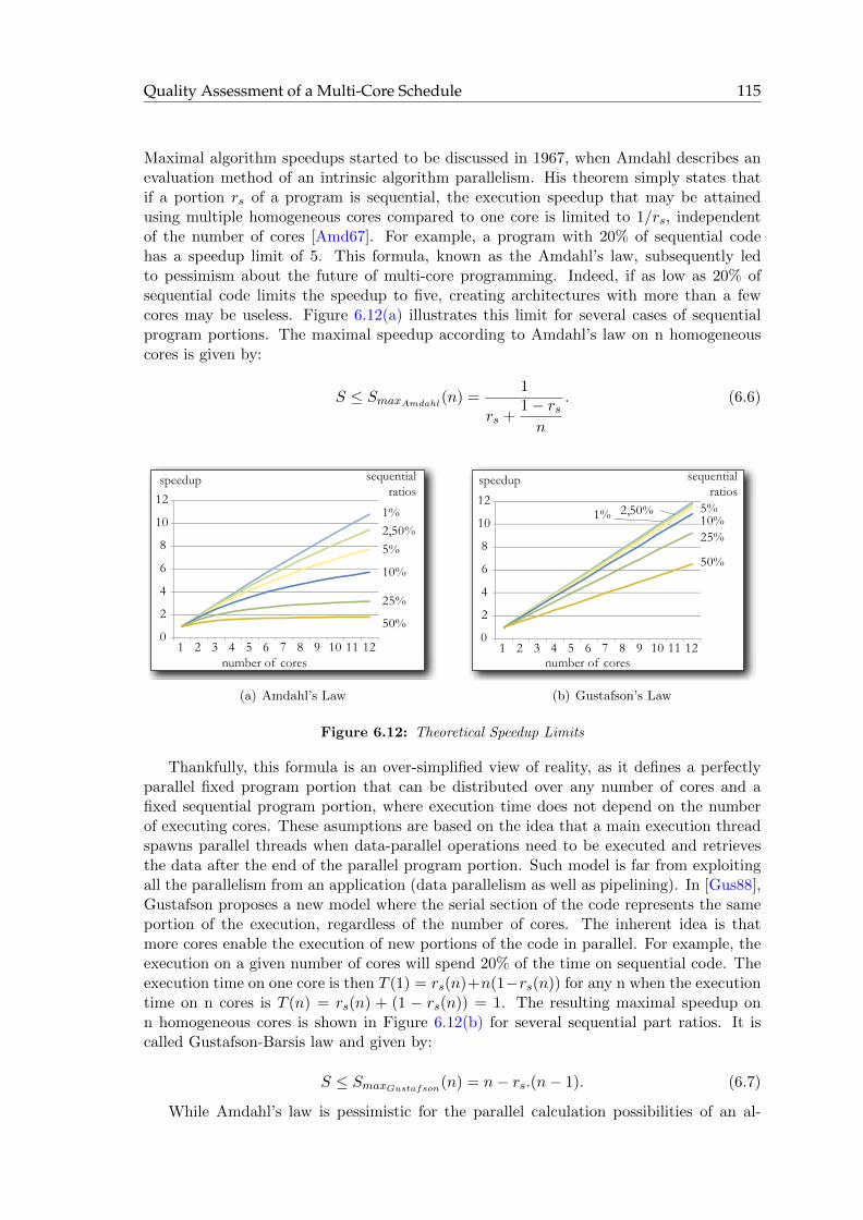
Quality Assessment of a Multi-Core Schedule 115
Maximal algorithm speedups started to be discussed in 1967, when Amdahl describes anevaluation method of an intrinsic algorithm parallelism. His theorem simply states thatif a portion rs of a program is sequential, the execution speedup that may be attainedusing multiple homogeneous cores compared to one core is limited to 1/rs, independentof the number of cores [Amd67]. For example, a program with 20% of sequential codehas a speedup limit of 5. This formula, known as the Amdahl’s law, subsequently ledto pessimism about the future of multi-core programming. Indeed, if as low as 20% ofsequential code limits the speedup to five, creating architectures with more than a fewcores may be useless. Figure 6.12(a) illustrates this limit for several cases of sequentialprogram portions. The maximal speedup according to Amdahl’s law on n homogeneouscores is given by:
S ≤ SmaxAmdahl(n) =
1
rs +1− rsn
. (6.6)
0
2
4
6
8
10
12
1 2 3 4 5 6 7 8 9 10 11 12
1%2,50%5%
10%
25%
50%
sequentialratios
speedup
number of cores
(a) Amdahl’s Law
0
2
4
6
8
10
12
1 2 3 4 5 6 7 8 9 10 11 12
1% 2,50% 5%10%25%
50%
speedup
number of cores
sequentialratios
(b) Gustafson’s Law
Figure 6.12: Theoretical Speedup Limits
Thankfully, this formula is an over-simplified view of reality, as it defines a perfectlyparallel fixed program portion that can be distributed over any number of cores and afixed sequential program portion, where execution time does not depend on the numberof executing cores. These asumptions are based on the idea that a main execution threadspawns parallel threads when data-parallel operations need to be executed and retrievesthe data after the end of the parallel program portion. Such model is far from exploitingall the parallelism from an application (data parallelism as well as pipelining). In [Gus88],Gustafson proposes a new model where the serial section of the code represents the sameportion of the execution, regardless of the number of cores. The inherent idea is thatmore cores enable the execution of new portions of the code in parallel. For example, theexecution on a given number of cores will spend 20% of the time on sequential code. Theexecution time on one core is then T (1) = rs(n)+n(1−rs(n)) for any n when the executiontime on n cores is T (n) = rs(n) + (1 − rs(n)) = 1. The resulting maximal speedup onn homogeneous cores is shown in Figure 6.12(b) for several sequential part ratios. It iscalled Gustafson-Barsis law and given by:
S ≤ SmaxGustafson(n) = n− rs.(n− 1). (6.7)
While Amdahl’s law is pessimistic for the parallel calculation possibilities of an al-

116 Enhanced Rapid Prototyping
gorithm, the Gustafson-Barsis law is optimistic and shows that Amdahl’s law was not astrict limit, as previously believed. With a sequential section of 20%, the Amdahl maxi-mal speedup on 10 cores is 3.6 while the Gustafson maximal speedup is 8.2. Amdahl andGustafson laws, as well as Karp-Flatt metric [KF90], are based on the very unrealisticidea that the middle-grain parallelism of algorithm is concentrated in perfectly parallelzones. With graphs of program execution, more realistic parallelism metrics can be usedas advised by Leiserson in [Lei05]. Contrary to the previous laws, Leiserson’s intent is onlyto evaluate the available parallelism present in the high-level model of the code; however,the figures are more reliable because they are based on algorithm properties that are moreprecise than parallel and sequential program sections.
6.6.2 Upper Bound of the Algorithm Speedup
It is important to evaluate the quality of the computed schedule. For that purpose, thespeedup increase that occurs as the number of cores is augmented is of interest. Forthis study, communication times are not considered because they greatly depend on thearchitecture. The only input for the evaluation of the possible speedup included in thisstudy is the algorithm. It is assumed that the architecture is homogeneous and has aninfinite speed media. The first limit that must be considered is the work length. The workis the sum of all actor execution times and corresponds to the algorithm latency on onecore T(1) (Section 6.4.2). Except in the exotic case of superlinear speedups which appearwhen the work decreases with the increasing number of cores, the work will be distributedon all n cores and so:
T (n) ≤ T (1)/n⇒ S ≤ Ssupwork= n. (6.8)
This speedup limit is a function of the number of available cores. Another general lim-itation can be found in the length of the span, i.e. the critical path when communicationsare ignored. Both work and span were shown to be calculable by the infinite homogeneousABC in Section 6.4.2. No matter how well the algorithm is parallelized, the latency cannot be reduced to less than the critical path. The critical path length T∞ adds a newconstraint on the speedup:
T (n) ≥ T∞ ⇒ S ≤ Ssupspan = T (1)/T∞. (6.9)
As these upper bounds have been defined, a minimum acceptable performance may beresearched.
6.6.3 Lowest Acceptable Speedup Evaluation
As compile-time scheduling computation is used with list scheduling and probabilistic re-finements, its performance should always be equal to or better than the basic “greedy”scheduler. The “greedy” scheduler executes actors as soon as they become available. Ateach time step, there are either more than n available actors, where n of them are dis-patched on the cores and the step is called complete or there are less than n availableactors, and they are all dispatched on the cores and the step is called incomplete. Gra-ham [Gra69] and Brent [Bre74] give an limit inferior to the latency that such a “greedy”scheduler can obtain using the Greedy Scheduling Theorem (GST):
T (n) ≤ T (1)
n+ T∞ ⇒ S ≥ SinfGST
=T (1)
T (1)
n+ T∞
. (6.10)

Quality Assessment of a Multi-Core Schedule 117
The proof of GST can be found in [Lei05]. If a result worse than GST is obtained,the compile-time scheduling process can not be considered successful. Again, this theoremdoes not take into account the communication times due to hardware constraints that canmake real schedules sub-optimal. From the previously defined upper and lower boundson speedup, a chart can be derived, displaying the optimality of an algorithm schedulelatency.
a
DSP1DSP2DSP3
5
1
5
5
4
1
2
1
b
c
d
e
f
g
h
j
(8)
(5)
(5)(5)
3
2
32
(3)
(5)
(8)
(5)
(3)
a bcd
ef
g
h i
0 10 20 30
Latency = 303 identical coresWork = 57Critical path = 22Speedup = 57/30 = 1.9
i(10)
1
j0
1
2
3
1 2 3 4 5 6 7 8
Current schedule
architecture-limitedzone
algorithm-limitedzone
bad schedule zone
unreachable zone
S sup
work
Ssup span
S inf GST
cores
speedup
Figure 6.13: Speedup Chart of an Example DAG Scheduling
Figure 6.13 displays the speedup optimality assessment of a small DAG schedulingprocedure. The DAG is annotated with its Deterministic Actors Execution Times (inbrackets) and the time cost of its transfers. To be efficient, the scheduling must be insidethe space delimited by the three curves. The best results are obtained when it is closestto the upper left corner. Moreover, depending on the number of cores, its parallelism iseither limited by the number of cores in the architecture (architecture-limited zone) or bythe degree of parallelism in the graph (algorithm-limited zone). In [Sin07], Sinnen definesthe Communication to Computation Ratio (CCR) as the sum of communication time costsdivided by the sum of computation time costs in a scheduled graph. Figure 6.13 makessense as long as CCR� 1 is in the tested schedule. This constraint is not a real problembecause CCR� 1 is also a condition for the implementation to be efficient.
6.6.4 Applying Scheduling Quality Assessment to Heterogeneous TargetArchitectures
The previous calculations were all based on homogeneous architectures but their use canbe extended to heterogeneous target architectures if certain precautions are taken. Thetarget architectures of this study (Section 5.1.1) have cores of homogeneous type c64x+that perform the majority of the operations in the application. The c64x+ core type mustbe set in the scenario as the main operator type. The parallelism of the cores with maintype can thus be studied in the quality assessment chart. The results are complicated bythe fact that coprocessors improve the speedup and increased communications degrade thespeedup. The number of cores in the speedup chart refer only to cores with main operatortype. The second precaution is that any actor executed by coprocessors must be forcedon that coprocessor to allow the specific study of the behavior of c64x+ cores.
In order to compute work and span, the infinite homogeneous ABC is run to simulatea UNC execution of the code (Section 6.4.2). It calculates the algorithm work using

118 Enhanced Rapid Prototyping
DAETs with software actors on maintype cores and hardware actors on their respectivecoprocessors. The span is different than the critical path length computed for the listscheduling because it does not take into account the transfers in the infinite homogeneousarchitecture. The span is computed by scheduling the graph on a UNC architecture withan infinite number of main .type cores and coprocessors with non-null loads.
Under these conditions, the speedup chart provides a quick evaluation of the optimalityof the main system cores under the constraint of fixed mappings. It can be used to evaluatewhether a lower granularity in the algorithm is necessary to extract more parallelism or,conversely, if certain actors should be clustered.
After this introduction of enhanced rapid prototyping features, the following chapterswill discuss the modeling of LTE for rapid prototyping and code generation.

CHAPTER 7
Dataflow LTE Models
7.1 Introduction
The objectives of rapid prototyping are introduced in Chapter 1. Figure 6.1 illustrates theprocess of rapid prototyping. Technical background on the subject is explored in Chapter4. In this chapter, models for the LTE rapid prototyping process are explained. From thesemodels, execution can be simulated and optimized using multi-core scheduling heuristicsand code can also be generated. The LTE models are novel and can complement thestandard documents for a better understanding of the LTE eNodeB physical layer. Aftera general view of the LTE model is given in Section 7.2, the three parts of the LTE eNodeBphysical layer are detailed in sections 7.3, 7.4 and 7.5. LTE rapid prototyping is processedby a Java-base framework which includes PREESM. The elements of this framework areintroduced in following sections.
7.1.1 Elements of the Rapid Prototyping Framework
The framework for rapid prototyping that was constructed during this thesis containsthree main elements: PREESM, Graphiti and SDF4J. The framework is illustrated inFigure 7.1 and detailed in [PPW+09]. All the blocks in Figure 7.1 except SDF4J areopen-source plug-ins for the Eclipse environment [ecl]. They can use and extend theadvanced functionalities of Eclipse in terms of graphical user interface and frameworkorganization. In the PREESM project, special attention is given to program tools thatwill be maintained in the long term, using encapsulation and design patterns [GHJV95](visitor, abstract factory, singleton, command...). Execution time of the different workflowelements is optimized to offer prototyping solutions as expediously as possible.
7.1.2 SDF4J : A Java Library for Algorithm Graph Transformations
The java library named SDF4J (Synchronous Dataflow for Java) manipulates dataflowgraphs and is available in Sourceforge [sdf]. This library can process SDF graphs (Section3.2) and its subsets (DAG...) as well as IBSDF (Section 3.4.2). It performs the algorithmgraph transformations called in the workflows, as explained in Section 6.2.3, includinghierarchy flattening, schedulability verification (Section 3.2), transformation into a DAG

120 Dataflow LTE Models
SDF4J
AlgorithmTransformation
Core
Multi-CoreScheduler
CodeGenerator
ArchitectureTransformation
Graphiti
GraphTransformation Library
Rapid PrototypingEclipse Plug-ins
Generic Graph Editor
Eclipse Plug-in
Eclipse Framework
Figure 7.1: An Eclipse-based Rapid Prototyping Framework
(Section 3.2.3), and clustering methods based on [Sar87]. SDF4J also contains a parserand a writer of GraphML files [BEH+01] to load and store its graphs.
7.1.3 Graphiti : A Generic Graph Editor for Editing Architectures,Algorithms and Workflows
Graphiti provides a generic graph editor and is completely independent from PREESM.It is written using the Graphical Editor Framework (GEF). The editor is generic in thesense that any type of graph may be represented and edited. Graphiti is routinely usedwith the following graph types and associated file formats : CAL networks [EJ03] [Jan07],S-LAM architectural representations stored in IP-XACT format (Section 5.2), SDF andIBSDF graphs stored in GraphML format and PREESM workflows (Section 6.2.3), storedin specific XML files.
The type of graph is registered within the editor by a configuration. A configurationis a structure that describes :
1. The abstract syntax of the graph (types of vertices and edges, and attributesallowed for objects of each type),
2. The visual syntax of the graph (colors, shapes, and so on),
3. Transformations from the file format in which the graph is defined to Graphiti’sXML file format G, and vice-versa (Figure 7.2).
Two kinds of input transformations are supported: from custom XML to GraphitiXML format and from text to Graphiti XML format (Figure 7.2). XML is transformedto XML using Extensible Stylesheet Language Transformation (XSLT [w3c]). The secondinput transformation parses the input text to its Concrete Syntax Tree (CST) representedin XML according to a LL(k) grammar by the Grammatica [graa] parser. Similarly, twokinds of output transformations are supported, from XML to XML and from XML to text.
Graphiti handles attributed graphs [JE01]. An attributed graph is defined as adirected multigraph G = (V,E, µ) where V the set of vertices, and E the multiset ofedges (there can be more than one edge between any two vertices). µ is a function µ :({G}∪V ∪E)×A 7→ U that associates instances with attributes from the attribute nameset A and values from U , the set of possible attribute values. A built-in type attribute isdefined so that each instance i ∈ {G} ∪ V ∪E has a type t = µ(i, type), and only admits

Proposed LTE Models 121
XML
Text XMLCST
XSLTtransformations
Gparsing
(a) reading an input file to G
G XSLTtransformations
XML
Text
(b) writing G to an output file
Figure 7.2: Input/output with Graphiti’s XML format G
attributes from a set At ⊂ A given by At = τ(t). Additionally, a type t has a visual syntaxσ(t) that defines its color, shape and size.
To edit a graph, the user selects a file and the matching configuration based on thefile extension is computed. The transformations defined in the configuration file are thenapplied to the input file and result in a graph defined in Graphiti’s XML format G asshown in Figure 7.2. The editor uses the visual syntax defined by σ in the configurationto draw the graph, vertices and edges. For each instance of type t the user can edit therelevant attributes allowed by τ(t) as defined in the configuration. Saving a graph consistsof writing the graph in G, and transforming it back to the input file’s native format.
Graphiti generates workflow graphs, IP-XACT and GraphML files that are the primaryinputs of PREESM rapid prototyping. The GraphML files containing the algorithm modelare loaded and stored in PREESM by the SDF4J library.
7.1.4 PREESM : A Complete Framework for Hardware and SoftwareCodesign
PREESM itself is composed of several Eclipse plug-ins (Figure 7.1). The core parsesand executes workflows, calling methods from the other plug-ins of PREESM. It includesthe SDF4J library and contains the classes of all objects exchanged in workflows (Section6.2.3). The core is the only compulsory element for PREESM. Other plug-ins can be addedto extend PREESM functionalities. The algorithm and architecture transformation plug-ins provide graph transformations to the workflow. The algorithm transformation plug-ingenerally calls SDF4J functionalities. The multi-core scheduler contains all the featuresdiscussed in Chapter 6. The code generation plug-in generates self-timed executable code(Section 4.4.1) from schedules provided by the multi-core scheduler. Code generation willbe extended in Chapter 8.
7.2 Proposed LTE Models
7.2.1 Fixed and Variable eNodeB Parameters
Certain parameters of an eNodeB do not change during its whole life span and otherparameters change every millisecond. For the rapid prototyping process, simulation usecases must be chosen that represent real-life execution cases. The compile-time and run-time actor scheduling must take into account the life spans of parameters and to managestatic parameters, no scheduling overhead should be introduced at run-time.
The duplex mode (Section 2.3.4) is a fixed parameter determined during the networkconstruction. The bandwidth of an eNodeB and the cyclic prefix mode (normal orextended) are also fixed network parameters. Once a frequency band has been boughtby an operator, the eNodeB is configured to exploit fully this bandwidth. The number
122 Dataflow LTE Models
of available subcarriers is consequently also a fixed parameter, as are the size of theFourier transforms in SC-FDMA and OFDMA encoding and decoding (Section 2.3.4).
The format and localization of the RACH preamble, as well as the number of roots andcyclic shifts (Section 2.4.5) are stable. These parameters depend only on the environmentof the eNodeB and are not permitted to vary over time because they must provide a stableaccess point for UEs. Thus, the RACH decoding has no variable parameters.
The number of antennas for uplink, downlink and PRACH is stable. The multipleantenna schemes for uplink and downlink are determined in the eNodeB (Sections 2.3.6,2.4.4 and 2.5.4). Each eNodeB may have a preferred multiple antenna scheme correspond-ing to its environment (rural and flat, mountainous, urban...) but a number of differentmodes are likely to be used depending on the channel quality of each user.
It is the highly variable parameters of an eNodeB that depend on the UE connections.In PUSCH, the number of UEs sending data changes every TTI of one millisecond(Section 2.3.4). The number of Code Blocks sent (Section 2.3.5) and the sizes ofthese Code Blocks also changes every TTI depending on the services accessed by eachUE (telephony, web...). The repartition of this data in the frequency band can differ foreach slot of 0.5 millisecond because of frequency hopping (Section 2.4.2). In PDSCH, thenumber of variables is approximately the same as in PUSCH but with an additional degreeof freedom in the number of transport blocks sent to a UE during a TTI. In PUSCH,with the exception of MU-MIMO, there is no spatial multiplexing so only one transportblock per TTI is transmitted (Section 2.4.4). In PDSCH, 2x2 spatial multiplexing can beemployed (Section 2.5.4) and a single UE can receive two transport blocks in one TTI.
The modulation and coding scheme (Section 2.3.5) is specific to each UE so willalso varies in every TTI. The transport block size and number of transport blocks for aUE determines for each TTI the quantity of data exchanged with the core network (Figure2.4).
As a consequence of these parameter variations, RACH preamble decoding is a staticoperation that can be studied entirely at compile-time while uplink decoding and downlinkencoding are highly variable over time. Despite these variations, case studies may be chosenso behavioral information can be extracted from the corresponding dataflow graphs atcompile-time. A typical use case is presented in next section.
7.2.2 A LTE eNodeB Use Case
In order to study LTE multi-core execution, typical use cases must be defined. We presenthere a typical eNodeB and its performance. The objective of this section is to explainthe important features that must be taken into account when evaluating LTE physicallayer performance. Considering a FDD eNodeB with 20MHz downlink and uplink and 100PRBs per slot, the system behavior can be evaluated using information given in Chapter2. A configuration of four transmission and four reception antenna ports (Section 2.3.6)is chosen for this eNodeB.
Uplink Performances
Firstly, considering the PUSCH with standard cyclic prefix, each PUSCH resource blockcontains 6 symbols∗12 subcarriers = 72 resourceelements; one additional symbol is usedas a reference symbol (Figure 2.17). Table 7.1 gives the capacity of Resource Elements(RE) and resource blocks in bits and deduces the raw bit rates for the current case. Thistotal data rate must be shared between all UEs. The base time unit for data allocation to

Proposed LTE Models 123
Table 7.1: Maximal Raw Bit Rates of Uplink Resources
ModulationScheme
bits/RE bits/PRB bits/pair ofPRBs
max raw bi-trate
QPSK 2 144 288 28.8 Mbit/s
16-QAM 4 288 576 57.6 Mbit/s
64-QAM 6 432 864 86.4 Mbit/s
a UE is a single TTI of one millisecond; thus it can be seen that a pair of PRBs containthe minimum amount of bits that can be allocated to a UE.
From these raw data rates, the multiple control overheads must be subtracted:
� The outer PRBs are reserved for PUCCH. This exact number is typically up to16 PUCCH regions, i.e. 16 PRBs per slot are kept for PUCCH ([STB09]). Itmay be noted that the modulation and coding scheme is different between PUSCHand PUCCH; thus the PUCCH raw bit rate cannot be directly deduced from thiscalculation.
� The rate matching process (Section 2.3.5) has a rate of “useful data” between 7.6%and 93%. The channel coding rate is linked to the chosen modulation scheme (Figure2.14(a)).
� The transmission of the PRACH channel requires part of the uplink bandwidth. Ina typical case of a cell with radius smaller than 14 km, a preamble of format 0 canbe allocated every 2 milliseconds. It results in 6 PRBs every 2 milliseconds, so usesapproximately 3% of the resources.
Thus, the maximal PUSCH data rate may be evaluated, including these overheads.Under ideal conditions where 64-QAM can be employed over the entire bandwidth with93% channel coding rate, a PUSCH data rate of 86.4 ∗ 0.93 ∗ 0.81 = 65Mbit/s can beattained. The CRCs and the overhead of the upper layers are not taken into account;these parameter also reduce the final bit rate available to the UEs IP layer. The uplinktransmission process is constructed to allow the LTE uplink data rate requirement of 50Mbit/s to be attained.
Downlink Performances
The downlink performance evaluation uses the table of transport block sizes in [36.09e]p.26. The transport block size (in bits) depends on the number of allocated PRBs, andon an index named ITBS (Index of Transport Block Size). Downlink Control Informa-tion (DCI, Sections 2.3.5 and 2.5.2) sent in PDCCH to a UE details the link adaptationparameters and determines the ITBS . From the ITBS , the maximal downlink data ratesfor a given modulation scheme, with 2x2 spatial multiplexing (2 transport blocks) can beevaluated. The results are shown in Table 7.2.
The displayed data rates target only PDSCH and include the control channel costs. Asabove, these maximal data rates are those of the physical layer. Upper layers will furtherreduce the effective data rate available to the IP layer of the UEs.
The following sections focus on models of multi-core execution for the physical layerof LTE eNodeBs. To study the system-level and the link-level data behavior of the LTE

124 Dataflow LTE Models
Table 7.2: Maximal Raw Bit Rates of PDSCH
ModulationScheme
ITBS bits/2TBs max raw bitrate
QPSK 9 31704 31.7 Mbit/s
16-QAM 15 61664 61.7 Mbit/s
64-QAM 26 149776 149.8 Mbit/s
downlink, an open source simulator under Matlab is provided by the Technical Universityof Vienna [MWI+09].
7.2.3 The Different Parts of the LTE Physical Layer Model
LTE physical layer decoding can be divided into three major actors: random accessdecoding, uplink decoding and downlink encoding. Uplink decoding and randomaccess decoding are frequency multiplexed in the same symbols but they are separated inthis study for two reasons: firstly, both actors are very costly, and are potentially paralleland secondly, while PRACH decoding is a completely static operation, uplink decodingexecution varies every millisecond. Thus studying each actor separately allows better andfast optimization.
The scale and granularity of the three actor descriptions must be defined (Section3.1.2). The scale is determined by the application. For PRACH decoding, the obviousscale results from a graph decoding a complete preamble sent over 1, 2 or 3 milliseconds.This preamble transmission time depends on preamble type. The latency of one RACHpreamble detection then is minimized. For uplink and downlink actors, graphs could beconstructed where each processes one symbol (decoding a 71.4 µs period) but this wouldintroduce too much low-level conditioning, including parameters with static patterns.
Another possibility would be to design uplink and downlink graphs representing oneentire frame (decoding 10 milliseconds) but this solution leads to very large graphs andHARQ puts latency constraint on subframe processing, not frame processing. Thus, thecorrect scale for uplink and downlink graphs is the time to process one subframe (1 millisec-ond). The granularity is chosen so that atomic actors (with no hierarchy) have relativelyclose execution times. A typical actor execution time is a few thousand of cycles. Inthe following sections, models of random access decoding, uplink decoding and downlinkencoding with user- selected scale will be presented.
7.3 Prototyping RACH Preamble Detection
Random Access Channel Preamble Detection (RACH-PD) consists of decoding the multi-plexed and non-synchronized messages from the UEs attempting to connect to the eNodeB(Section 2.4.5). The preamble is transmitted on the Physical RACH (PRACH) channelover a specified time-frequency resource, denoted as a slot, available with a certain cycleperiod and a fixed bandwidth of six PRBs. Within each slot, a guard period is reservedat each end to maintain time orthogonality between adjacent slots.
The method used to execute RACH-PD is the hybrid time-frequency domain approachdescribed in [STB09] p.449 and [JMB]. With this method, the PRACH message decodercan start before the whole message has been received. It uses small FFTs and is basedon downsampling and anti-aliasing. The Power Delay Profile (PDP) is then computed. It

Prototyping RACH Preamble Detection 125
consists of the norm of the periodic correlation of each Zadoff-Chu sequence (Section 2.4.3)with the received sequence. A peak in the Power Delay Profile indicates the detection ofa signature and the location of the peak provides the timing advance of the transmittingUE, i.e. the propagation time between UE and eNodeB. Peak detection must take intoaccount the noise in received samples; thus, the noise is estimated and the threshold forpeak detection depends on this estimation. To compute the correlation between receivedsignal and signatures, the convolution with complex conjugate is used.
The case studied in this section assumes a RACH-PD for a cell size of 115 km. This isthe largest cell size supported by LTE and is also the case requiring the most processingpower. According to [36.09c], preamble format#3 is used with 21,012 complex samplesas a cyclic prefix, followed by a preamble of 24,576 samples followed by the same 24,576samples repeated. In this case, the slot duration is 3 milliseconds which gives a guardperiod of 21,996 samples.
Noise floorestimation
Peaksearch
Noise floorestimation
Peaksearch
Noise floorestimation
Peaksearch
Noise floorestimation
Peaksearch
Sum of the energiesof the 8
preambles copies(64 repetitions)
...
.........
...
.........
...
Noise floorestimationNoise floorestimationNoise floorestimationNoise floorestimation
Noise floorestimationNoise floorestimationNoise floorestimationNoise floorestimation
Noise floorthreshold
(64 repetitions)
Route preamble 3frequency response
Complex conjugation
Zero padding IFFT | |2
Route preamble frequency response
Complex conjugation
Zero padding IFFT | |2
Route preamble 1frequency response
Complex conjugation
Zero padding IFFT | |2
BPF DFT
Subcarrier demapping
Pre-processing
Preamble processing: Antenna 4 first copy of the preamble
...
...
Route preamble 3frequency response
Complex conjugation
Zero padding IFFT | |2
Route preamble 2frequency response
Complex conjugation
Zero padding IFFT | |2
Route preamble 1frequency response
Complex conjugation
Zero padding IFFT | |2
BPF DFT
Subcarrier demapping
Pre-processing
Preamble processing: Antenna 3 first copy of the preamble
...
...
Route preamble 3frequency response
Complex conjugation
Zero padding IFFT | |2
Route preamble 2frequency response
Complex conjugation
Zero padding IFFT | |2
Route preamble 1frequency response
Complex conjugation
Zero padding IFFT | |2
BPF DFT
Subcarrier demapping
Pre-processing
Preamble processing: Antenna 2 first copy of the preamble
...
...
Circular correlation(64 repetitions)
Route preamble 3frequency response
Complex conjugation
Zero padding IFFT | |2
Route preamble 2frequency response
Complex conjugation
Zero padding IFFT | |2
Route preamble 1frequency response
Complex conjugation
Zero padding IFFT | |2
FIR DFT
Subcarrier demapping
Pre-processing
Preamble processing:Antenna 1 first copy
of the preamble
...FS
...
Route preamble 3frequency response
Complex conjugation
Zero padding IFFT | |2
Route preamble frequency response
Complex conjugation
Zero padding IFFT | |2
Route preamble 1frequency response
Complex conjugation
Zero padding IFFT | |2
BPF DFT
Subcarrier demapping
Pre-processing
Preamble processing: Antenna 4 second copy of the preamble
...
...
Route preamble 3frequency response
Complex conjugation
Zero padding IFFT | |2
Route preamble 2frequency response
Complex conjugation
Zero padding IFFT | |2
Route preamble 1frequency response
Complex conjugation
Zero padding IFFT | |2
BPF DFT
Subcarrier demapping
Pre-processing
Preamble processing: Antenna 3 second copy of the preamble
...
...
Route preamble 3frequency response
Complex conjugation
Zero padding IFFT | |2
Route preamble 2frequency response
Complex conjugation
Zero padding IFFT | |2
Route preamble 1frequency response
Complex conjugation
Zero padding IFFT | |2
BPF DFT
Suber demapping
Pre-processing
Preamble processing: Antenna 2 second copy of the preamble
...
...
Circular correlation(64 repetitions)
Route preamble 3frequency response
Complex conjugation
Zero padding IFFT | |2
Route preamble 2frequency response
Complex conjugation
Zero padding IFFT | |2
Route preamble 1frequency response
Complex conjugation
Zero padding IFFT | |2Subcarrier demapping
Pre-processing
Preamble processing:Antenna 1 second copy
of the preamble
...FIR DFTFS
...
Delay(800μs)Delay(800μs)Delay(800μs)Delay(800μs)
RF
Figure 7.3: RACH-PD Algorithm Model
As per Figure 7.3, the algorithm for the RACH preamble detection can be summarizedin the following steps [JMB]. The dataflow graph in Figure 7.3 illustrates the actorscontained by the IBSDF description.
1. After cyclic prefix removal, the pre-processing actor isolates the RACH band-width by shifting the data in frequency (Frequency Shifting, FS) and band-passfiltering it with downsampling (Finite Impulse Response, FIR). The data is thentransformed into the frequency domain (DFT) and the subcarriers of interest areselected (subcarrier demapping).
2. Next, the circular correlation actor correlates data with pre-stored preambleroot sequences in order to discriminate between simultaneous messages from severalusers. The complex conjugates of the root sequences are directly retrieved from

126 Dataflow LTE Models
memory; consequently, the correlation step only costs a complex multiplication. Thecircular correlation actor also applies an IFFT to return to the temporal domain andcalculates the energy of each root sequence correlation. The more roots there are,the more circular correlations are processed. This is why cyclic shifts are used whenpossible to reduce the number of root (Section 2.4.5).
3. Then, the noisefloor threshold actor collects these energies and estimates thenoise level for each root sequence.
4. Finally, the peak search actor detects all signatures sent by the users in the currenttime window. It additionally evaluates the transmission timing advances, correlatedwith the distance of the transmitting UEs. The timing advances are sent to theMAC layer which then transmits each value to the appropriate UE to command acompensation.
In general, there are three parameters of RACH which are highly dependent on the cellsize, and may be varied: the number of receive antennas, the number of root sequences andthe number of repetitions of the same preamble. The case with 115 km cell size implies 4antennas, 64 root sequences, and 2 repetitions, as shown in Figure 7.3.
The goal of rapid prototyping of a RACH-PD can be to determine, through simulation,the number of c64x+ cores needed by the architecture to manage the 115km cell RACH-PDalgorithm. The RACH-PD algorithm behavior is described as a IBSDF graph in PREESM.The algorithm can be easily adapted to different eNodeB use cases by tuning the graphparameters. The IBSDF description is derived from the representation in Figure 7.3. Aftera total flattening (Section 3.4.2), the graph contains 2209 vertices. This high number maybe reduced by merging actors and/or reducing the flattening degree. Placing these actorsonto the different cores by hand would be greatly time-consuming. As seen in Section 7.1.4the rapid prototyping PREESM tool provides automatic scheduling, avoiding the problemof manual placement.
A significant point to note is that RACH decoding has an absence of feedback edgeand a total independence of preceding preamble detection iterations. In the IBSDF graphdescription of RACH-PD, the graph is actually acyclic and the SDF to DAG transformationhas no effect on its topology. The graph also displays a high parallelism that can beextracted at compile-time. Indeed, its topology depends only on parameters that are fixedfor the lifespan of an eNodeB . Thus, no assignment step is needed at run-time to optimallyexecute RACH-PD on a distributed architecture. The parallelism can be evaluated interms of span, length and potential speedup using the quality assessment chart fromSection 6.6, computed in PREESM. However, this chart does not take communicationcosts or heterogeneity into account. An architecture exploration is needed to perform aprecise and complete hardware and software codesign.
Architecture Exploration
The four architectures explored are shown in Figure 7.4. The cores are all homoge-neous Texas Instrument c64x+ DSP running at 1 GHz [TMS08]. The connections aremade via DMA-driven routes. The first architecture is a single-core DSP such as theTMS320TCI6482. The second architecture is dual-core, with each core similar to that ofthe TMS320TCI6482. The third is a tri-core and is equivalent to the tci6488 (Section5.1.1). Finally, the fourth architecture is a theoretical architecture for exploration only,as it is a quad-core. The exploration goal is to determine the number of cores required

Prototyping RACH Preamble Detection 127
to run the random RACH-PD algorithm in a 115 km cell and how to best distribute theoperations on the given cores.
PE1
DMA
PE2PE1 PE2
DMA
PE3
PE1
PE3
DMA
PE4
PE1 PE2
1 2 43
Figure 7.4: Four architectures explored
To solve the deployment problem, each operation is assigned an experimental timing(in terms of CPU cycles) in the scenario. These timings are measured with deploymentsof the actors on a single C64x+. Since the C64x+ is a 32-bit fixed-point DSP core, thealgorithms must be converted from floating-point to fixed-point prior to these deployments.The EDMA is modeled as a parallel node controlled by a DMA (Chapter 5) transferringdata at a constant rate and with a given set-up time.
Loosely timedApproximately timedAccurately timed
Real-time limit of 4ms
1 core
3 cores + EDMA
4 cores + EDMA
2 cores + EDMA
Figure 7.5: Timings of the RACH-PD algorithm schedule on target architectures
The PREESM automatic scheduling process is applied for each architecture. Theworkflow used is close to that of Figure 6.4. The simulation results obtained are shown inFigure 7.5. The list scheduling heuristic is used with loosely-timed, approximately-timedand accurately-timed ABCs. Due to the 115 km cell constraints, preamble detection mustbe processed in less than 4 milliseconds (Section 2.4.5).
The experimental timings were measured on code executions using a tci6488. Thetimings feeding the simulation are measured in loops, each calling a single function withL1 cache activated. For more details about C64x+ cache, see [TMS08]. This warm cachecase represents the application behavior when local data access is ideal and so will lead toan optimistic simulation. The RACH application is well suited for a parallel architecture,as the addition of one core reduces the latency dramatically. Two cores can process thealgorithm within a time frame close to the real-time deadline with loosely and approxi-mately timed models but high data transfer contention and high number of transfers makethe dual-core architecture not sufficient when accurately timed model is used.
The 3-core solution is best: its CPU loads (less than 86% with accurately-timed ABC)are satisfactory and do not justify the use of a fourth core, as can be seen in Figure 7.5.The high data contention in this case study justifies the use of several ABC models; simplemodels are used for fast results and more complex models are then employed to correctlydimension the system.

128 Dataflow LTE Models
7.4 Downlink Prototyping Model
Encoding the LTE downlink consists of preparing the different data and control channelsand multiplexing them in the radio resources. Depending on the amount of control neces-sary in a subframe, the 1, 2 or 3 first symbols carry the control channels (Section 2.5.2).The remaining resources are shared between data channel (PDSCH), broadcast channelsand reference signals . To encode the LTE downlink, the baseband processing retrieves thedata Transport Blocks (TB) from the MAC layer (Figure 2.6) and applies channel codingto them. Control channels and reference signals are then generated and multiplexed withthe data channel prior to MIMO encoding.
Symbols #1 to 13Symbol #0
PBCH
PMCH
UE #2 to NUE #1
PDCCHPCFICHPHICH
PDSCHPBCHPMCH
...
1 PRB =7 symbols ×
12 sub-carriers
frequency
time
PDSCH TB #2 (if Spatial Multiplexing)PDSCH TB #1 CB #2 to M
CB #1
Add
C
RC C
B
Turb
oE
ncod
ing
Rate
Mat
chin
g
Cod
e Bl
ock
Con
cate
natio
n
Scra
mbl
ing
Cod
e Bl
ock
Segm
enta
tion
Add
CRC
TB
Con
stel
latio
nM
appi
ng
Laye
r/A
nten
naM
appi
ng &
Pr
ecod
ing
From Layer 2
PDCCH
PCFICH
PHICH
RS
PSS
SSS
ResourceMapping
RF
Antenna Stream #2 to A
IFFT
Inse
rtC
P
Antenna Stream #1
Channel Encoding
Figure 7.6: Downlink Decoding
A dataflow graph for encoding rapid prototyping is shown in Figure 7.6. It is composedof three parts:
� during channel encoding the PDSCH data bits are transformed into symbols (Sec-tion 2.5.2). First, a Cyclic Redundancy Check (CRC) is added to each TB. The TBis then segmented into Code Blocks (CB) and each CB also receives a CRC. TheseCRCs enable the detection of errors when a UE decodes PDSCH. The resulting codeblock with CRC is Turbo-Encoded and rate-matched (Section 2.3.5) to introduce

Uplink Prototyping Model 129
the exact amount of desired redundancy in the binary information for Forward Er-ror Correction (FEC). Then, the encoded code-blocks are concatenated before beingscrambled and constellation mapped. Scrambling spreads the redundant data evenlyto protect it against the frequency-selective air channel and a constellation mappingis chosen among QPSK, 16-QAM and 64-QAM. The data is now composed of sym-bols. The decisions are not shown in Figure 7.6 but all decisions (Hybrid ARQparameters for retransmission, Modulation scheme, Antenna mapping mode,and soon) are sent by the MAC layer. Finally, the symbols are mapped to layers and thelayers are precoded and mapped to antenna ports (Section 2.5.4). Layer mappingand precoding depend on the multiple antenna PDSCH mode (spatial multiplexingor not, open or closed loop) chosen by the MAC layer.
� during the control and broadcast channels generation, channel symbols aregenerated to be multiplexed with PDSCH. The primary control channel, PDCCH,as well as PCFICH and PHICH channels are mapped to the first 1, 2 or 3 symbols ofthe encoded subframe (Section 2.5.2). Certain Reference Symbols (RS) also appearin these first symbols. PBCH broadcast channel values are generated only if thecurrent subframe contains cell information broadcast, which is the case once everyframe of 10 milliseconds. PBCH values are multiplexed with PDSCH, multicastchannel PMCH, RS and Synchronization Symbols (PSS and SSS, Section 2.5.5) inthe remaining 13, 12 or 11 symbols of the subframe.
� in the front-end, each complex value of the previously mentioned physical channelsis associated with a Resource Element (RE) in the Resource Mapping procedure.Resource mapping is a bottleneck in the application because all symbols from allUEs must be collected prior to forwarding them to the rest of the front-end. AnIFFT is then applied to convert each symbol of each antenna port into the timedomain for transmission and a cyclic prefix is inserted between each symbol to reduceinter-symbol interferences (Section 2.3.2).
The PDSCH processing dominates the computation cost of other downlink physicalchannels. It is for this reason that it is divided into actors while PHICH generation isseen as a single “black box”. When described in an IBSDF, the number of repetitions ofeach actor (per TB, per CB, per UE, per antenna port...) is determined by the number ofdata tokens flowing between the different actors in the graph. Like the RACH-PD IBSDFdescription, the downlink encoding graph is fairly parallel and is already an acyclic graph.Unlike the RACH-PD IBSDF description, its topology depends on certain parameters(number of receiving UEs, number of TBs, size of these TBs and number of CBs) thatvary each subframe because the subframe is the basic time unit for UE allocation (Section2.3.2). It must be noted that only typical or worst-case downlink test cases can be studiedin PREESM.
7.5 Uplink Prototyping Model
The uplink model is divided into PUCCH and PUSCH models. Decoding the PUCCHuplink control channel is a complex and potentially parallel operation. Contrary to thePDCCH encoding that may be represented as a single actor, as in Figure 7.6, the PUCCHmodel is presented as a complex graph. It may be noted that the PUCCH and PUSCHgraphs process the same raw symbols received by the antennas.

130 Dataflow LTE Models
7.5.1 PUCCH Decoding
Decoding PUCCH consists of extracting resource blocks at the edge of the bandwidth fromthe raw data received by the antenna and then processing them to retrieve the uplinkcontrol bits. The localization of PUCCH in the bandwidth was explained in Section 2.4.2.
Symbol #1 to 13Symbol #0
Antenna Stream #2 to A
Freq
uenc
ySh
ift
Rem
ove
CP
FFT
(204
8)
PUSC
H/C
CH
Dem
appi
ng
Antenna Stream #1
PUCCH
PUSCH1 PRB =
7 symbols ×12 sub-carriers
...
PUCCH PRB #2 to NPUCCH PRB #1
Pre-Processing
Conjugated ZC Sequence
...
IDFT
-12
frequency
time
DemuxUE
Decode UEPUCCH
ACK/NACK/SR/DTX(+CQI/PMI/RI only format 2)
Decoder dependingon PUCCH format1/1a/1b/2/2a/2b
RF
Front End
Per UE
Figure 7.7: PUCCH Decoding
A dataflow graph for decoding PUCCH is displayed in Figure 7.7. The PUCCH de-coding consists in three distinct steps:
� The front end is common to PUCCH and PUSCH. The uplink subcarriers are fre-quency shifted by half the width of a subcarrier, i.e. by 7.5 kHz, to reduce distortionson the central resource blocks from the local oscillator. A frequency shift of 7.5 kHzis thus first applied to the received signal to compensate for this shift. The problemdoes not appear in downlink because one subcarrier (named d.c. subcarrier) is punc-tured (Figure 2.21). In uplink, the same solution would worsen the PAPR and thusincrease UE power consumption ([STB09] p.353). The CP is then removed and thesymbols are transformed to the frequency domain by a FFT. The FFT size dependson the bandwidth (Table 2.1) with a maximum of 2048 points in the 20 MHz band-width case with 1200 subcarriers. Finally, resource elements from the band edgesare used in the PUCCH decoding procedure while the center elements are used inthe PUSCH decoding.
� The pre-processing step demultiplexes the PUCCH information from multiple UEswhich was transmitted over the same resources using CDM (Section 2.4.1). For theUE, CDM encoding consists of multiplying, in the frequency domain, the data witha Zadoff-Chu Sequence of length 12 and with a given cyclic shift. Thus, it is possiblefor two UEs using the same ZC sequence with different cyclic shift to use the samePBR. For each PRB, there are twelve possible cyclic shifts. To decode the CDM,a multiplication with the Zadoff-Chu sequence is applied followed by a DFT of thesize of a PRB.
� In the decoder step, the UE data is then demultiplexed and, depending on thePUCCH block format, certain information is extracted, using Reed-Muller decoding

Uplink Prototyping Model 131
to decode CQI (Section 2.3.5). ACK is reported by the UE in the case of a correctdownlink reception; NACK for a failed downlink reception (when the CRC indicatederrors in transmission) and DTX means that the UE did not even detect in PDCCHthat it had data to receive in PDSCH.
The information extracted from PDCCH is reported to the MAC layer, which controlsthe downlink communication. The PDCCH can also contain an uplink Scheduling Request(SR) when a UE requires more PUSCH resources.
7.5.2 PUSCH Decoding
PUSCH decoding is the most complex graph in the LTE eNodeB physical layer model. Itcontains seven parts and is illustrated in Figure 7.8:
Antenna Stream
#2 to A
DFT
Antenna Stream #2 to A
PUCCH
PUSCH1 PRB =
7 symbols ×12 sub-carriers
...
frequency
time
... ChannelSounding
Frequency OffsetEstimation
SRS Symbol
DM RS Symbols
PilotDemodulation
IDFT
Windowing &Noise Floor
Removal
Antenna Stream
#1
Multi-AntennaEqualization
IDFT
Frequency Dom
ainSym
bol Processing
Channel E
stimation
ChannelEstimates
per Symbol
UE #2 to N
Freq
uenc
y O
ffse
tC
ompe
nsat
ion
UE #1
Channel Decoding
Con
stel
latio
nD
emap
ping
Des
cram
blin
gD
eint
erle
avin
g
Dem
ultip
lexi
ng
CB #2 to MCB #1
Rate
Dem
atch
ing
HA
RQC
ombi
ning
Turb
oD
ecod
ing
CB
CRC
Che
ck
Cod
e Bl
ock
Con
cate
natio
n
TB C
RC C
heck
TBUE #1
...
Decoding of Control Information
Interpolation
DataSymbols
To Layer 2
Symbol #1 to 13Symbol #0
Antenna Stream #2 to A
Freq
uenc
ySh
ift
Rem
ove
CP
FFT
(204
8)
PUSC
H/C
CH
Dem
appi
ng
Antenna Stream #1
Front End
RF
Antenna Stream #1
Data/DM RS/SRSDemux
Time domain symbols from every antenna ports
Figure 7.8: PUSCH Decoding
� The front end is common to PUCCH and PUSCH and was explained in Section7.5.1. It outputs the physical resource blocks dedicated to PUSCH in frequencydomain.

132 Dataflow LTE Models
� The data/DM RS/SRS demultiplexer separates the reference signals from thedata resource elements.
� The channel sounding processes the SRS symbol 13 and sends sounding informa-tion to the MAC layer (Section 2.4.1). This information is used to schedule UEs inthe subsequent subframe.
� the frequency offset estimation evaluates the Doppler effect experienced by eachUE data TB due to UE velocity. The estimation uses the two reference DM RSsymbols 3 and 10 (Section 2.3.1). The frequency offset is then transmitted to theMAC layer and influences the channel decoding.
� the channel estimation processes the ZC sequences from the two DM RS sym-bols to compute the Channel Impulse Response (CIR). The pilot subcarriers fromdifferent UEs are first separated. They are then transformed into time domain byan IDFT. The DM RS signal is synchronized and noise removed. Finally, the sig-nal is transformed back into frequency domain, the CIR is evaluated and is linearlyinterpolated to find the CIR of each of the eleven data symbols.
� The frequency domain symbol processing first combines the data from differentantenna ports, equalizing them (Section 2.3.2) and using either MRC or MIMO de-coding, depending on the UE multiple antenna scheme employed (Section 2.3.6). Aswith channel estimation, the data from each UE is processed independently becauseit may have different MCS that other UEs. The data is then transformed into timedomain by an IDFT. It may be noted that the equalizer processes the data from allantenna ports together. Moreover, after Frequency Domain Symbol Processing, thedata from all the symbols must be gathered for joint processing. These two bottle-necks limit functional parallelism, introducing additional causality in the system butthey cannot be avoided.
� The channel decoding step is approximately the inverse operation of the downlinkchannel encoding explained in Section 7.4. The transport block values of each UEare processed, extracting bits from the time-domain symbols. The frequency offsetdue to the Doppler effect is compensated and data is demapped, descrambled anddeinterleaved. A second demultiplexing of data and control is necessary at this pointbecause certain control values can be multiplexed with data if PDCCH capacityis insufficient ([STB09] p.398). Each CB is then dematched and combined withany previous HARQ repetition. A hidden feedback edge exists because code blocksfrom previous iterations of the graph are maintained in the MAC layer for futurecombination with the subsequent repetition. After Turbo decoding, the CRC ischecked to verify whether data was lost and a new HARQ repetition is necessary.CBs are finally gathered and the TB CRC is checked.
Contrary to the downlink part, only one TB per UE can be received in a subframebecause no spatial multiplexing other than MU-MIMO is allowed. In order to obtain acorrect simulated decoding latency, the IBSDF graph must account for the fact that eachsymbol is received with a delay of 1/14 millisecond more than the preceding one. As thereis no notion of time in IBSDF and it is the scenario alone that introduces timings foractors, a “trick” must be used to include these delays. This “trick” consists of introducinga fake processing element in the architecture, which this study will call Antenna Interface(AIF). A “dummy” delay actor is added to the algorithms, assigned to AIF, associated

Uplink Prototyping Model 133
with a 1/14 millisecond timing on AIF in the scenario. This actor is preceded by another“dummy” actor whose use is to repeat the delay. A feedback edge on the delay actorensures the order of execution of its instances. The original graph and its form aftertransformation to a single rate graph are shown in Figure 7.9. The delay from the first“dummy” actor must be subtracted from the latency. The same technique can be used inthe downlink model to receive transport blocks at disparate times.
AIFReal Architecture
containing Core 1 and Core 2
Delay141
11
(71428 ns)(0 ns)
Delay_Repeat
Delay Delay Delay Delay Delay Delay Delay Delay Delay Delay Delay Delay Delay Delay
Frequency Shift11 ...
DR D
D
D
D
D
FS
FS
FS
FS
FS
...
...
...
...
...
FSFS
FSFS
FSFS
FSFS
FSFS
FSFS
FSFS
AIFCore 1Core 2
SDF single rate SDF
11
1
1
1
11
1
1
1...
Figure 7.9: Introducing Delays in a IBSDF Description to Simulate Events
It may be noted that the data rate of both uplink and downlink communicationsbetween baseband processing and antenna ports can be a challenge. For a 20MHz cellwith 30.72 MHz sampling rate and 4 antenna ports and with complex data of 16-bitreal and imaginary parts, the antenna data rate is almost 4Gbit/s in both directions.Consequently, the hardware antenna interface needs to support very high data rates. Thecomplex AIF data exchanges can be studied at system-level using PREESM and S-LAMContention Nodes, without considering all the details of implementation.
Of course, when the RACH-PD, downlink and uplink graphs are all prototyped to-gether, the result is an extensive graph. Synchronization can then be specified for thereception time of the downlink transport blocks and also the reception time of the uplinksymbols, using the “trick” presented above. This chapter presented LTE modelization forrapid prototyping. The next chapter explains code generation from LTE dataflow graphdescriptions.

134 Dataflow LTE Models
CHAPTER 8
Generating Code from LTE Models
8.1 Introduction
Literature on automatic multi-core code generation was reviewed in Section 4.5 andscheduling strategies in Section 4.4.1. In this section, generated code execution schemesare defined, detailing how code is generated from a given scheduling strategy. Code gen-eration for RACH-PD (Section 8.2), PUSCH (Section 8.3) and PDSCH (Section 8.4) isthen explained. Combining the three dataflow paths is discussed finally in Section 8.5.
8.1.1 Execution Schemes
In [BW09], Bell and Wood advise programmers on multi-core programming. The architec-tures they study are the same DSPs targeted by this study. Their recommended methodfor parallelizing applications is based on a test-and-refine approach and is manual withsteps that are different from those of Figure 4.2. The report then presents the two execu-tion schemes which form the basis of distributed code generation: the master/slave schemeand the dataflow scheme. Instead of “dataflow” scheme, the terminology “decentralizedscheme” will be used to avoid confusion with dataflow MoC. An execution scheme differsfrom a MoC in that it defines the architecture of a running code, with run-time systemconsiderations that MoCs do not model.
� The master/slave scheme, illustrated in figure 8.1(a), consists of a centralizedexecution control code in a master task that posts actors to slaves tasks. In thismodel, actors are often called jobs but this term is usually used for actors which areloosely coupled with respect to each other. A master or a slave task can be entirelysoftware-defined or have certain parts that have been hardware accelerated. Eachtask can be locally contained in threads controlled by an OS or be the only computa-tion of an operator. The centralized control code simplifies the efficient distributedexecution of the various applications, i.e applications are dominated by the controlcode rather than data because these applications require a centralized knowledge ofthe control values to efficiently reconfigure the parallel execution. [BW09] advisesuse of the master/slave scheme for RLC and MAC Layers of telecommunication sys-tems (Section 2.2.2), as these layers are always dominated by the control code. For

136 Generating Code from LTE Models
instance, in LTE, the eNodeB MAC scheduler is a complex control-dominated op-eration which varies greatly depending on the state of the communication (numberand distance of the connected users, quality of the channels, MIMO schemes, and soon). A master can either be an “intelligent” unit, posting actors where they will bemost efficiently executed or a simple pool of actors that the slaves monitor for actoravailability.
� The decentralized scheme, illustrated in figure 8.1(b), consists of independenttasks which wait for input data, process it and send it without use of a globalexecution arbitrator. This scheme corresponds to a “real” dataflow implementationwhere computation is triggered solely by data arrival. Naturally, this scheme is wellsuited to dataflow application implementation and [BW09] advises the use of thedecentralized scheme when implementing the physical layer of telecommunicationsystems. However, as the uplink and downlink streams of the LTE eNodeB physicallayer are quite balanced between data and control, the most appropriate executionscheme for these algorithms is clearly a mix of the master/slave and decentralizedschemes.
controlcode
master task
slave task
Actor A
slave task
Actor Bslave task
Actor DActor C
assigns
assigns
assigns
finished
(a) Master/Slave Execution Scheme
task
Actor A
task
Actor D
Actor Ctask
Actor B
triggers trigger
s
triggers
(b) Decentralized Execution Scheme
Figure 8.1: Execution Schemes
As centralized resources in distributed architectures usually form system bottlenecks,the centralization of the master in the master/slave scheme is a real issue. Hierarchicalapproaches can reduce the problem. In a hierarchical multi-core scheduler, a top-levelscheduler assigns a pool of operators to a part of the application. The assignment andscheduling of that subsystem is then managed by a lower-level scheduler which is locatedelsewhere. Pools of operators can overlap; in this case, a time-sharing scheme is necessaryfor each shared operator. This is usually performed by the top-level scheduler reconsideringits choices periodically. System introspection (monitoring operator activity) can also beused to choose when to reconsider top-level assignment. [HjHL06] is an example of such ahierarchical scheduler with two levels.
Both master/slave and decentralized schemes can be used to generate code fromdataflow MoCs. However, the most appropriate execution scheme depends on the chosenscheduling strategy (Section 4.4.1). Static-assignment, self-timed and fully static schedul-ing strategies can be implemented using both master/slave and decentralized schemes.However, all three strategies execute the assignment step at compile time to simplify run-time and avoid the need for a centralized control code. Consequently, the most efficientexecution scheme for static-assignment, self-timed and fully static scheduling strategies isthe decentralized scheme. Conversely, the fully dynamic scheduling strategy necessitates

Static Code Generation for the RACH-PD algorithm 137
a run-time actor assignment. This strategy demands the centralization of either the exe-cution control code or the pool of actors.Therefore, the master/slave scheme is the onlypossible execution scheme for this scheduling strategy. The relation between schedulingstrategies and execution schemes is illustrated in Figure 8.2 and the two pairs of strate-gy/scheme that this study uses for LTE are highlighted.
natural associationspossible but sub-optimal associations
Scheduling Strategies
fully dynamicstatic-assignment
self-timedfully static
Execution Schemes
master/slave
decentralized scheme
Figure 8.2: Possible Associations of Scheduling Strategies to Execution Schemes
A master element containing a multi-core scheduler is the central piece of a multi-coreRTOS. Such a system, if highly optimized, could improve embedded multi-core program-ming by offering an abstraction of heterogeneous computing not available today.
8.1.2 Managing LTE Specificities
For each dataflow graph, the right scheduling strategy needs to be selected dependingon the variable behavior of target application and architecture. Once the schedulingstrategy is chosen, the execution scheme is chosen, as seen in Figure 8.2. For the RACH-PD algorithm, the couple self-time scheduling/decentralized scheme is the most suitablesolution due to static system behavior (Section 7.2) as well as the fact that the executiontime of the target operators cannot be precisely known. For the processing of controlchannels (PUCCH, PDCCH...), the limited costs of the actors mean that a static self-timescheduling/decentralized scheme is a good solution because adaptive scheduling wouldincur an unacceptably high overhead.
Conversely, the very high variability of the PUSCH and PDSCH algorithms in additionto their high computing cost make a more complex strategy, such as master/slave executionscheme, desirable.
Using quasi-static multi-mode schedule selection [HL97], all possible combinations ofparameters must be scheduled and a tradeoff found at compile-time, which would be im-possible with the PUSCH and PDSCH because of the high number of cases (Section 8.3.4).PUSCH and PDSCH necessitate the use of run-time adaptive scheduling instead of multi-mode compile-time scheduling. These two code generation ideas are developed in thefollowing sections.
8.2 Static Code Generation for the RACH-PD algorithm
The RACH-PD is a static algorithm, so it can be efficiently parallelized using the PREESMframework code generation.
8.2.1 Static Code Generation in the PREESM tool
The PREESM tool code generation uses the self-timed scheduling strategy (Section4.4.1) and the decentralized execution scheme. Many principles are adapted fromthe AAM methodology and incorporated into the tool [GS03]. The code generated by

138 Generating Code from LTE Models
the PREESM tool is analogous to a coordination code (Section 3.2). The host code andcommunication libraries (Section 3.2) must be manually coded.
op2
DMA
op3
op1
tci8488 S-LAM modelwith c64x+ operators
Scheduler
Code G
eneration
XSL Transform
ation
TI Code C
omposer C
ompiler
communication libraries and actor code
op1.xml op1.c op1.exe
op3.xml op3.c op3.exe
op2.xml op2.c op2.exe
IDL prototypes
Schedule
Algorithmand scenario c64x+.xsl
Figure 8.3: Code generation Procedure on a tci6488
To generate code statically, the static scheduling of the input algorithm on the inputarchitecture must have been defined. A typical PREESM workflow performing code gen-eration is displayed in Figure 6.4. For each operator, the generated code consists of aninitialization phase and a loop endlessly repeating the part of the algorithm graph assignedto this operator. Special code loops are generated from IBSDF descriptions for the non-flattened and repeated hierarchical actors in order to obtain a compact code [PBPR09].Each atomic actor generates a function call on its assigned core as explained in Section6.2.1. The function call prototype is defined in an IDL file. The path of the IDL files isa parameter of the code generation workflow node. From the deployment informationpro-vided by the scheduler, the code generation module creates a generic representation of thecode in XML. This code is then XSLT-transformed to produce the specific code for thetarget. The code generation flow for a tri-core tci6488 target processor (Section 5.1.1) isillustrated in Figure 8.3.
The XML generic code representation is illustrated by an example in Figure 8.4, whichshows the XML code file generated for the operator op1 of Figure 8.3. The file containsa static buffer allocator, a computation thread and a communication thread. It alsocontains an operator type which indicates which XSLT transformation file to use whengenerating the coordination code, in this case “c64x+.xsl”. The two threads communicatevia statically allocated shared buffers and semaphores. The communication thread controlsthe DMA and waits for completion of transfers, while the computation thread executescode in parallel, calling functions with parameters of type constant or buffer.
PREESM currently supports the C64x and C64x+ based processors from Texas In-struments with a DSP-BIOS Operating System [dsp] and the x86 processors with a Win-dows Operating System. Device-specific code libraries have been developed to managethe communications and synchronizations between the target cores [PAN08]. The XSLTtransformation generates calls to the appropriate predefined communication library, whichare dependent on the route type and on the names of the communication nodes betweenoperators in the S-LAM architecture model (Chapter 5),. The inter-core communicationschemes supported include TCP/IP with sockets, Texas Instruments EDMA3 [PAN08]and RapidIO link [rap].
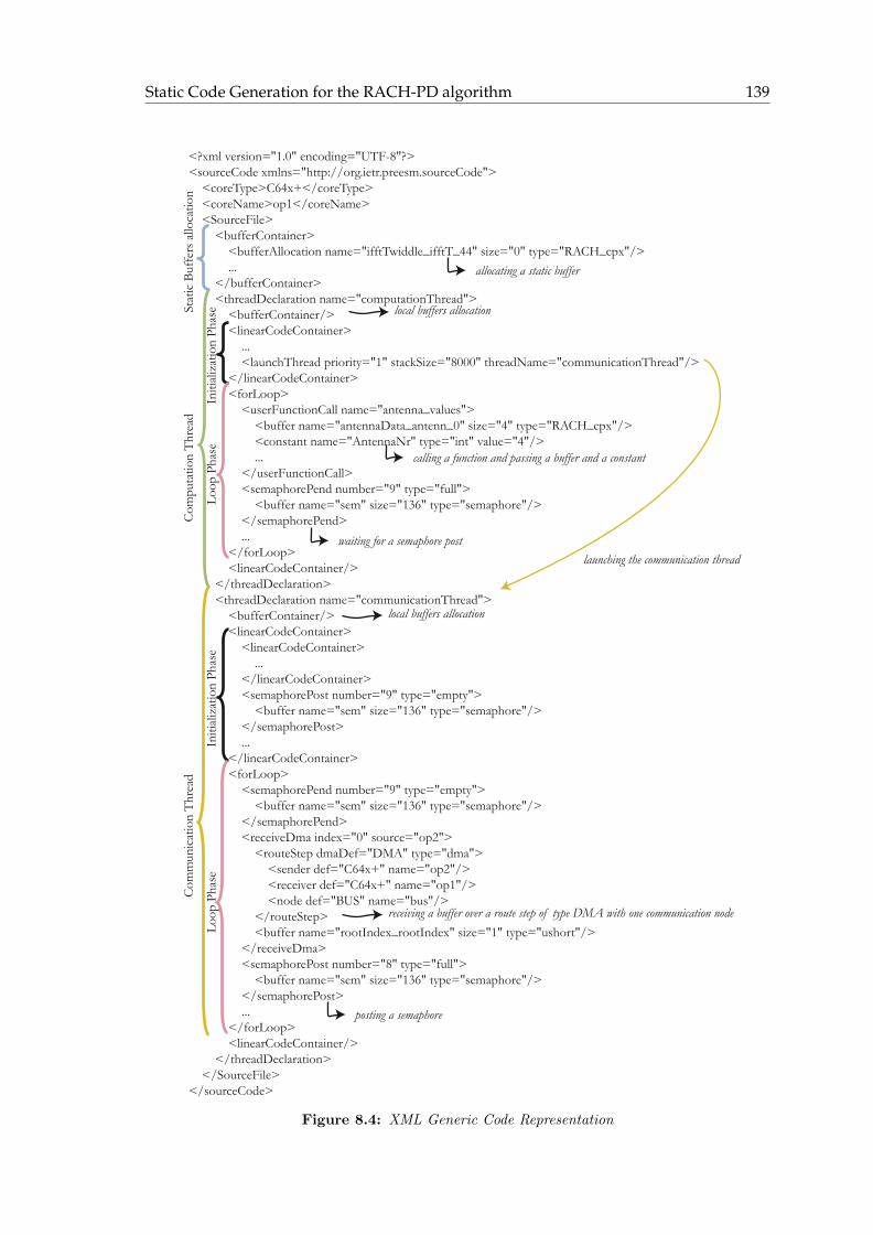
Static Code Generation for the RACH-PD algorithm 139
<?xml version="1.0" encoding="UTF-8"?><sourceCode xmlns="http://org.ietr.preesm.sourceCode"> <coreType>C64x+</coreType> <coreName>op1</coreName> <SourceFile> <bufferContainer> <bufferAllocation name="ifftTwiddle_ifftT_44" size="0" type="RACH_cpx"/> ... </bufferContainer> <threadDeclaration name="computationThread"> <bufferContainer/> <linearCodeContainer> ... <launchThread priority="1" stackSize="8000" threadName="communicationThread"/> </linearCodeContainer> <forLoop> <userFunctionCall name="antenna_values"> <buffer name="antennaData_antenn_0" size="4" type="RACH_cpx"/> <constant name="AntennaNr" type="int" value="4"/> ... </userFunctionCall> <semaphorePend number="9" type="full"> <buffer name="sem" size="136" type="semaphore"/> </semaphorePend> ... </forLoop> <linearCodeContainer/> </threadDeclaration> <threadDeclaration name="communicationThread"> <bufferContainer/> <linearCodeContainer> <linearCodeContainer> ... </linearCodeContainer> <semaphorePost number="9" type="empty"> <buffer name="sem" size="136" type="semaphore"/> </semaphorePost> ... </linearCodeContainer> <forLoop> <semaphorePend number="9" type="empty"> <buffer name="sem" size="136" type="semaphore"/> </semaphorePend> <receiveDma index="0" source="op2"> <routeStep dmaDef="DMA" type="dma"> <sender def="C64x+" name="op2"/> <receiver def="C64x+" name="op1"/> <node def="BUS" name="bus"/> </routeStep> <buffer name="rootIndex_rootIndex" size="1" type="ushort"/> </receiveDma> <semaphorePost number="8" type="full"> <buffer name="sem" size="136" type="semaphore"/> </semaphorePost> ... </forLoop> <linearCodeContainer/> </threadDeclaration> </SourceFile></sourceCode>
Com
mun
icat
ion
Thr
ead
Com
puta
tion
Thr
ead
Stat
ic B
uffe
rs a
lloca
tion
Initi
aliz
atio
n Ph
ase
Initi
aliz
atio
n Ph
ase
Loop
Pha
seLo
op P
hase
launching the communication thread
allocating a static buffer
calling a function and passing a buffer and a constant
waiting for a semaphore post
posting a semaphore
receiving a buffer over a route step of type DMA with one communication node
local buffers allocation
local buffers allocation
Figure 8.4: XML Generic Code Representation
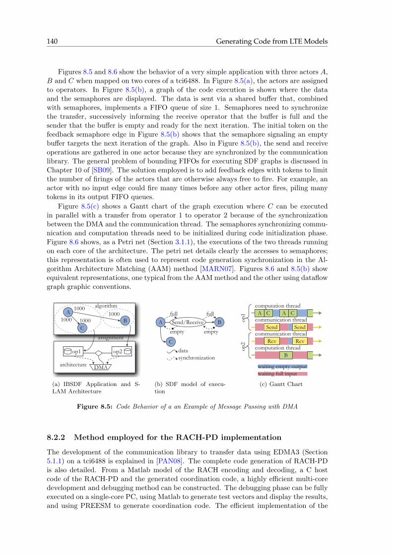
140 Generating Code from LTE Models
Figures 8.5 and 8.6 show the behavior of a very simple application with three actors A,B and C when mapped on two cores of a tci6488. In Figure 8.5(a), the actors are assignedto operators. In Figure 8.5(b), a graph of the code execution is shown where the dataand the semaphores are displayed. The data is sent via a shared buffer that, combinedwith semaphores, implements a FIFO queue of size 1. Semaphores need to synchronizethe transfer, successively informing the receive operator that the buffer is full and thesender that the buffer is empty and ready for the next iteration. The initial token on thefeedback semaphore edge in Figure 8.5(b) shows that the semaphore signaling an emptybuffer targets the next iteration of the graph. Also in Figure 8.5(b), the send and receiveoperations are gathered in one actor because they are synchronized by the communicationlibrary. The general problem of bounding FIFOs for executing SDF graphs is discussed inChapter 10 of [SB09]. The solution employed is to add feedback edges with tokens to limitthe number of firings of the actors that are otherwise always free to fire. For example, anactor with no input edge could fire many times before any other actor fires, piling manytokens in its output FIFO queues.
Figure 8.5(c) shows a Gantt chart of the graph execution where C can be executedin parallel with a transfer from operator 1 to operator 2 because of the synchronizationbetween the DMA and the communication thread. The semaphores synchronizing commu-nication and computation threads need to be initialized during code initialization phase.Figure 8.6 shows, as a Petri net (Section 3.1.1), the executions of the two threads runningon each core of the architecture. The petri net details clearly the accesses to semaphores;this representation is often used to represent code generation synchronization in the Al-gorithm Architecture Matching (AAM) method [MARN07]. Figures 8.6 and 8.5(b) showequivalent representations, one typical from the AAM method and the other using dataflowgraph graphic conventions.
AB
10001000
algorithm
op1
DMA
op2
C1000 1000
assignment
architecture
(a) IBSDF Application and S-LAM Architecture
A BSend/Receivefull full
empty empty
datasynchronization
C
(b) SDF model of execu-tion
waiting empty outputwaiting full input
A
Send
B
A
Send
Rcv Rcv
C Ccomputation thread
communication thread
communication thread
computation thread
op1
op2
(c) Gantt Chart
Figure 8.5: Code Behavior of a an Example of Message Passing with DMA
8.2.2 Method employed for the RACH-PD implementation
The development of the communication library to transfer data using EDMA3 (Section5.1.1) on a tci6488 is explained in [PAN08]. The complete code generation of RACH-PDis also detailed. From a Matlab model of the RACH encoding and decoding, a C hostcode of the RACH-PD and the generated coordination code, a highly efficient multi-coredevelopment and debugging method can be constructed. The debugging phase can be fullyexecuted on a single-core PC, using Matlab to generate test vectors and display the results,and using PREESM to generate coordination code. The efficient implementation of the

Static Code Generation for the RACH-PD algorithm 141
EndLoop
EndLoop
init
PostFull
PendEmpty
Post Empty
Pend Full
Communicationthread
Computationthread
Begin Loop
EndLoop
EndLoop
init
Post Full
PendEmpty
Post Empty
PendFull
Communicationthread
Computingthread
Begin Loop
BeginLoop
Begin Loop
A BSend Receive
C
Op1.xm
l
Op2.xm
l
Figure 8.6: Petri Net of Execution of the Application in Figure 8.5(a)
embedded multi-core deployment is then generated seamlessly. This method, illustratedin Figure 8.7, was successfully applied to RACH-PD during this thesis. It can be dividedinto six steps:
PREESM descriptions
Matlab golden reference
PREESM-generated coordination C code
Host C code optimizedwith c64x+ intrinsics
Intrinsics equivalentcode in C
Matlab engine calls
Matlab plottingfunctionalities
SignalReference
Difference
Matlab-generated headers
Performances
Debug
x86 project
c64x+ project
Figure 8.7: Method for the RACH-PD Algorithm Implementation.
1. RACH-PD functions are written in C, inspired by a Matlab “golden” code whichencodes and decodes the PRACH channel. Each C function of the RACH-PD em-bedded code is hand-written, adding c64x+ intrinsics to optimize for speed. Intrin-sics specify assembly calls in a C code. Each function is then instrumented and runindependent of target to collect execution timestamps and allow evaluation of theircost.
2. PREESM generates two coordination codes from the IBSDF description of RACH-PD illustrated in Figure 7.3 and two S-LAM architecture models: a single-core x86and the targeted multi-core embedded platform. The x86 architecture will serve fordebugging phase and the target for the implementation. The actor timings previouslymeasured are used to simulate the execution while scheduling the graph.
3. Matlab encodes an input signal containing RACH preambles and then decodes it.It generates large header files in C code containing buffers with the data at several

142 Generating Code from LTE Models
steps in the decoding process, which are displayed in Figure 7.3, such as before andafter FIR, before and after correlation, before and after IFFT, and so on.
4. The code is run on a x86, adding C reference code for each c64x+ intrinsic andlinking to the Matlab engine for displaying the results in Matlab. The decodedsignal is contained in a Matlab-generated header. At each decoding step, a separateheader is generated by Matlab, and then the golden reference and the embeddedsolution are plotted using Matlab engine. Code errors and insufficient data accuracyare clearly visible in the plots, which can thus be used to debug the code.
5. communication libraries are hand-written and then debugged for the target (alter-natively, appropriate communication libraries may be retrieved if a previous projecthas used the same architecture).
6. Maintaining the identical host code but switching the coordination code, the RACH-PD is run on the target architecture to test its speed and accuracy of its results. Boththe intrinsic equivalent C code and the Matlab engine calls are then removed fromthe embedded project. No deadlock will appear at this point, as data dependenciesare handled during only automatic scheduling.
The above method has several benefits. Firstly, the code can be debugged withoutconsideration of parallel programming problems. Secondly, the debugging phase is fasterthan debugging with the target board because it involves no cross-compilation. Lastly,the parallelism has been entered into the PREESM framework which facilitates the re-deployment of the algorithm on new architectures. These advantages make static codegeneration a powerful tool for creating embedded multi-core code.
Code has been generated and tested for the RACH-PD algorithm. The resulting imple-mentation is deadlock-free but needs many manual tweaks to reduce its synchronizationand memory consumption and the final result is compatible with the simulated resultsfrom Figure 7.5 in terms of cadence (a cadence under 4 millisecond is obtained) but notin terms of latency. Some memory and synchronization optimizations are still needed inPREESM to obtain automatically an optimized code.
The static code generation process is efficient only if the actor times are relativelystable and the coordination topology is absolutely stable. This is the case for RACH-PDbut not for PUSCH decoding and PDSCH encoding. In the next section, a technique toautomatically schedule PUSCH on multi-core embedded systems is developed.
8.3 Adaptive Scheduling of the PUSCH
The underlying goal of adaptive scheduling is to create the central part of an efficientmulti-core RTOS for signal processing applications on heterogeneous architectures. Anadaptive scheduler needs to schedule its application efficiently with very little overhead.The implemented system is dedicated to a specific task. Consequently, the schedulercan adapt at compile time or during system launch to the system specificities and runefficiently afterwards. The adaptive scheduler implements a fully dynamic schedulingmethod and is an element of the master entity in a master/slave execution scheme. Adifference of the adaptive scheduler when compared to usual operating systems is that theadaptive scheduler manipulates actors instead of threads and should not need preemption,if actors are small enough, to respect application real-time constraints. Context switchingis thus useless for adaptive scheduling and deadlocks or race conditions do not exist.

Adaptive Scheduling of the PUSCH 143
In Section 4.4, adaptive scheduling approach was introduced. Adaptive schedulingis a fully dynamic scheduling method which assigns actors to operators at run-time andorders them using simple heuristics. Processing the LTE PUSCH in the eNodeB consistsof receiving the multiplexed data from connected UEs, decoding it and transmitting it tothe upper layers of the standard stack (Section 7.5). Depending on the number of activeUEs and on their instantaneous data rates, the decoding load may vary dramatically.A multi-core adaptive scheduler has capacity to recompute a schedule for the algorithmevery millisecond. One important function of adaptive scheduler is to maintain low uplinklatency. The LTE standard has strict constraints in terms of latency, limiting the availabletime for both uplink and downlink processing. The scheduler uses a graph modelingtechnique, as during the rapid prototyping phase, to determine the execution timing fromthe DAET of each actor on each operator. The schedule is determined after an “on-the-fly”simulation of the application execution. The next section introduces the PUSCH modelfor run-time scheduling.
8.3.1 Static and Dynamic Parts of LTE PUSCH Decoding
The PUSCH decoding operation (Figure 7.8) can be divided in two parts :
1. The static part: FFT front end processing and multiple antenna MinimumMean Square Error (MMSE) equalization. The parameters of these two op-erations (number of receive antennas, Frequency Division Duplex (FDD) or TimeDivision Duplex (TDD), bandwidth, and so on) are fixed during run-time. TheCyclic Prefix (CP) is removed, the frequency is shifted by 7.5 kHz as stipulated bythe 3GPP LTE standard, the symbols are converted into frequency domain by aFast Fourier Transform (FFT) and equalized using received reference signals. Thedata from up to four antennas is then combined and the subcarriers are reordered.Finally, an Inverse Discrete Fourier Transform (IDFT) reconverts the data back intothe time domain per user basis.
2. The dynamic part: channel decoding. For this operation, the parameters (numberof connected UEs, number of allocated Resource Blocks, modulation order, and soon) are highly variable during run-time. The multi-core scheduling of this dynamicpart must be adaptive.
The first and static part of processing can be represented as an IBSDF graph anddemonstrates a high level of parallelism. Consequently, the corresponding self-timed par-allel schedule can be processed at compile time using PREESM [PPW+09], which willalso generate a self-timed code similar to that generated for RACH-PD (Section 8.2). Themulti-core scheduling of the second and dynamic part needs to be adapted at run-timeto the varying parameters. A discussion of the constraints on these varying parametersfollows in the next Section.
8.3.2 Parameterized Descriptions of the PUSCH
The parameters of PUSCH decoding are specified in the eNodeB MAC layer. They areavailable at least 1 millisecond before the start of the decoding. This property makes pa-rameterized dataflow (Section 3.4.1) particularly suitable for describing PUSCH decodingbecause this millisecond allows the construction of an execution graph and the subsequentsearch for an efficient multi-core schedule using this graph.

144 Generating Code from LTE Models
The most common use of parameterized dataflow is to describe an algorithm in a hi-erarchical PSDF graph where init and sub-init phases φi and φs modify topology andactor parameters at different levels. Such a PSDF description of the PUSCH decoding isdisplayed in Figure 8.8. In this usage, the static part is not developed because it is par-allelized at compile-time (Section 8.3.1). The dynamic part is simplified compared withthe graph displayed in Figure 7.8: actors have been merged to reduce the final size of thegraph. Figure 8.8 is divided into two actors at top level: the convergence actor thatgathers data from all subframe symbols and the ChannelDecoding actor. The top-levelinitialization phase φi, is executed once per graph invocation (i.e. once per millisecond),and initializes parameters carrying the maximum number of Code Blocks (CB) per UE,and the maximum size of the CBs. In the sub-init phase φs, the number of UEs is retrievedfrom the MAC layer before each graph execution. The channel decoding actor is repeatednb UE times, as many times as there are UEs sending data in the subframe, as a conse-quence of token productions and consumptions. The channel decoding actor contains ahierarchy with five actors. The keepCurrentTones actor filters the subcarriers used fordata transmission and transmits the resultant subcarriers to the perUEProcessing whichprocesses the frequency offset compensation, channel decoding, constellation demapping,descrambling, deinterleaving and demultiplexing. The BitProcessing actor gathers ratedematching and HARQ combining information while the Turbo Decoding actor asso-ciates turbo decoding with CB CRC checking. Finally, the CRCCheck actor checks theCRC of the TB. At each invocation of ChannelDecoding, which occurs for each UE, thenumber of CBs is modified as well as the size of these CBs. For a topology parameter tobe modified before each iteration of the graph, it must be modified in the sub-init graphφs of ChannelDecoding to be executed before each execution of the body φb. Some actorsparameters are also modified in φs, such as code rate, modulation, MU-MIMO mode.
static part
SDF
convergence ChannelDecoding
init subInit PSDF Top
max_CBs_per_UE*nb_UE max_CBs_per_UE
Not repeatedmax_CBs_per_UE; max_CB_size
init subInit ChannelDecoding
KeepCurrentTones PerUEProcessing
nb_CB
BitProcessing Turbo Dec CRCCheck
code_rate; modulation; MU-MIMO_mode; CB_sizeRepeated nb_UE times
nb_CB nb_CB 1 1 1 1 nb_CB
nb_UE
Figure 8.8: PSDF Description of the Uplink.
In all the LTE graphs of the current study, there is no feedback path in the physicallayer. The SDF graph in Figure 8.8 is a Directed Acyclic Graph (DAG, Section 3.2.3).Knowing all UE and CB parameters in advance of a subframe allows the global reconfig-uration of the PUSCH graph instead of reacting locally to the variations of parameters insub-init graphs such as in Figure 8.8. The benefit of such a global reconfiguration is toprovide a system view of subframe decoding and to enable a simulation of the code execu-tion on a heterogeneous multi-core architecture using the compile-time methods presentedin Section 4.4. To achieve a global graph, patterns of token production and consumptionare used as in Parameterized Cyclo Static Dataflow Graphs (PCSDF) 3.3. A run-timesystem cannot handle the Basis Repetition Vector (BRV) computation of a PCSDF graphto instantiate the actors. The input model of the adaptive scheduler is thus reduced to

Adaptive Scheduling of the PUSCH 145
acyclic graphs and called Parameterized Cyclo Static Directed Acyclic Graph (PCSDAG).This is not a new model; it is a subset of the Parameterized CSDF model. Compared withthe Parameterized CSDF, the PCSDAG has been simplified and has no cycle. It containsonly a single vertex without input edge and the number of firings of this vertex is fixed to1.
stat
ic p
art
SDF
convergence
PCSDAG
max_CBs_per_UE*nb_UEmax_CBs_per_UE
Not repeated max_CBs_per_UE;max_CB_size
init subInit
KeepCurrentCBs PerUEProcessing
nb_UE;(nb_CB)
BitProcessing Turbo Dec CRCCheck
(code_rate); (modulation); (MU-MIMO_mode);(CB_size)
(nb_CB) 1 1 1 1 (nb_CB)(nb_CB)
Figure 8.9: PCSDAG Description of the Uplink.
A PCSDAG description of the LTE PUSCH decoding is shown in Figure 8.9. Both datatoken production and consumption of each PCSDAG edge is set by the MAC scheduler.The token production and consumption can either be a single integer value or a pattern ofinteger values. The PCSDAG has no hierarchy but the parameter (nb CB) is a templatewhich provides the number of CB for each UE, and all actor parameters are now templateswhich assign its own parameters: nb CB = {nb CB(UE1), nb CB(UE2), nb CB(UE3)...}to each CB. For example, a consumption of the number of CBs per UE can contain thepattern {10, 5, 3, 1, 1}, meaning that the actor will consume 10 data tokens on the firstfiring, 5 on the second and so on. 1 millisecond before each subframe, all production andconsumption patterns are set by the MAC scheduler. The PCSDAG can then be extendedinto a single rate DAG (Section 3.2.3) and the resulting single rate DAG is scheduled.The DAETs of the LTE PUSCH graph actors also depend on pattern parameters set bythe MAC scheduler. The domain of nb UE is between 0 and 100 UEs (ignoring PUCCH)because each pair of PRBs can be associated with a different UE and the domain of eachpattern element in nb CB is between 1 and 13 CBs. PCSDAG can model LTE PUSCHdecoding in a very compact way.
In the next section, the architecture model of the adaptive scheduler is explained.
8.3.3 A Simplified Model of Target Architectures
The processors targeted by this study are the heterogeneous multi-core DSPs introduced inSection 5.1.1 and boards interconnecting several of them. They include the 6-core tci6486and the 3-core tci6488. Combinations of these DSPs (interconnected between test boardswith RapidIO serial links for instance) are also targeted architectures. The dataflow graphscheduling techniques naturally handle heterogeneity in data links and operators, treatingtargets with coprocessors, different DSP frequencies and different communication media.For example, the tci6488 includes a turbo decoding coprocessor that can perform theForward Error Correction (FEC) [STB09] decoding part of the PUSCH processing.
Using S-LAM (Chapter 5) in the adaptive scheduler would not be realistic in terms ofmemory and computing cost. Therefore, a very simple architecture model is used, In thismodel, the DAET of actors in the single rate DAG are linked to operator types, enablingoperator heterogeneity. A matrix is created where each oriented pair of source and sinkoperators is associated with a transfer speed in Gbytes/s. This matrix is displayed inFigure 8.10 and its results are compared to that of S-LAM for an example consisting ofone tci6486 and one tci6488.

146 Generating Code from LTE Models
tci6488_1tci6488_2tci6488_3tci6486_1tci6486_2tci6486_3tci6486_4tci6486_5tci6486_6
tci64
88_1
tci64
88_2
tci64
88_3
tci64
86_1
tci64
86_2
tci64
86_3
tci64
86_4
tci64
86_5
tci64
86_6
022
0.1250.1250.1250.1250.1250.125
202
0.1250.1250.1250.1250.1250.125
220
0.1250.1250.1250.1250.1250.125
0.1250.1250.125
022222
0.1250.1250.125
202222
0.1250.1250.125
220222
0.1250.1250.125
222022
0.1250.1250.125
222202
0.1250.1250.125
222220
data ratesin GBytes/sGEM1
GEM2
GEM3
EDMA3
SCR2 GBytes/s
RIO
0.12
5 G
Byte
s/s
GEM1
GEM2
GEM3
GEM4
GEM5
GEM6
EDMA3
SCR
2 GBytes/s
tci6488
tci6486
Figure 8.10: Target Architecture Example in S-LAM and Adaptive Scheduler Matrix Model: atci6488 and a tci6486 Connected with a RapidIO Serial Link.
3 CBs2 CBs
5 CBs4 CBs
7 CBs6 CBs
8 CBs
1 CB 1 allocation pattern; 1 UE max
3 allocation patterns; 3 UEs max
7 allocation patterns; 5 UEs max11 allocation patterns; 6 UEs max
15 allocation patterns; 7 UEs max
22 allocation patterns; 8 UEs max
100 CBs50 CBs25 CBs 1958 allocation patterns; 25 UEs max
204226 allocation patterns; 50 UEs max190569292 allocation patterns; 100 UEs max
CB per UE
UEs2 allocation patterns; 2 UEs max
5 allocation patterns; 4 UEs max
...
Figure 8.11: The problem of allocating CBs to UEs is equivalent to integer partitions representedhere in Ferrer diagrams.
8.3.4 Adaptive Multi-core Scheduling of the LTE PUSCH
An obvious solution to efficiently schedule a dynamic algorithm onto a heterogeneousarchitecture is to schedule all possible configurations at compile-time and then switchbetween the pre-computed schedules at run-time. The limits of such an approach are nowanalyzed.
The Limits of Pre-computed Scheduling
Assigning a given number of CBs to UEs is a similar problem to partitioning the numberof CBs into a sum of integers. The problem of integer partitioning is illustrated by Ferrerdiagrams in Figure 8.11. Given a number NCB of CBs to assign, a Ferrer diagram givesthe possible number of different allocation configurations p(NCB), i.e. the possible numberof different graphs to schedule and map for a given quantity of CBs. The number of CBsNCB allocated every millisecond also varies between 0 and NCBMAX
. In Section 2.3.4,the maximum number of pairs of PRBs per subframe was shown to be a constant foreach eNodeB and is fixed between 6 and 100 depending on the LTE system bandwidth.NCBMAX
is equal to the maximum number of pairs of PRBs per subframe because PRBpair is the minimum resource released to a code block. The total number of different

Adaptive Scheduling of the PUSCH 147
possible graphs for a given eNodeB PUSCH is:
P (NCBMAX) =
NCBMAX∑i=1
p(i). (8.1)
For the simplest case of a 1.4MHz LTE system bandwidth with only a maximum of6 CBs to allocate, the number of possible graphs is 29. It is feasible to pre-computeand store the scheduling of these 29 graphs. However, the number of graphs increasesexponentially with NCB; the still relatively simple case of 3MHz with a maximum of 12CBs generates 271 graphs. Considering that for P (50) = 1295970, it can be concludedthat the scheduling of all LTE PUSCH cases with bandwidth higher than 3MHz cannotrealistically be statically scheduled.
It must be noted that the above calculation of cases for each bandwidth only takes intoaccount topology modifications and not execution time modifications due to the variablesize of the CBs. The next section explains an adaptive scheduler that can efficientlyschedule PUSCH despite topology and CB size variations.
Structure of the Adaptive Multi-core Scheduler
The adaptive multi-core scheduler algorithm is illustrated in Figure 8.12. There is aninitialization phase that generates the PCSDAG object from a manual description andpre-computes the graph parameter expressions. The following processing steps are calledeach millisecond when the MAC scheduler changes the CB allocation. These schedulersteps consist of 2 operations:
� The graph expansion which transforms the PCSDAG into a single rate DAG withshape dependent on the PCSDAG parameters.
� The list scheduling algorithm which maps each actor in the single rate DAG toan operator (core or coprocessor) in the architecture.
The goal of the initialization step of the adaptive scheduler is to maximally reduce theloop step complexity. The expressions of the PCSDAG edge productions and consump-tions are then parsed and converted into a Reverse Polish Notation (RPN) stack using theShunting-yard algorithm [Dij60]. RPN specifies the order of expression evaluation in an ef-ficient bracket-less expression. This technique allows the adaptive scheduler to manipulateefficiently the PCSDAG patterns, which is essential in a run-time scheduler.
Graph Expansion
List Scheduling
Initialization
from LTE Layer 2
PCSDAGsrDAG Schedule
to Runtime
PCSDAG parametersAdaptive Scheduler
< 1ms
archi
Figure 8.12: Adaptive multi-core scheduling steps: graph expansion and list scheduling steps arecalled in a loop every millisecond.
The output of the adaptive scheduler feeds a run-time procedure. This procedure mayimplement a multi-core API (OpenCL [opea], Multi-core Association [mca]). The sum ofgraph expansion and list scheduling execution times must stay under 1 millisecond for thescheduler to be an approach of interest in LTE PUSCH processing. These two operationsare detailed in the following Sections.

148 Generating Code from LTE Models
Adaptive Expansion of PCSDAG into Single Rate DAG
A single rate DAG (Section 3.1.2) is a graph with no cycle, in which each edge has equaldata production and consumption. All single rate DAG actors are instances of PCSDAGactors. Each single rate DAG actor is fired only once.
Figure 8.13 gives four examples of single rate DAG graphs generated from the expansionof the PCSDAG in Figure 8.9 with different allocation schemes. The number of (possible)vertices in a single rate DAG may be calculated by:
V = 2 + 3 ∗ nb UE + 2 ∗NCB. (8.2)
Thus, for the PUSCH example, the maximal size of the corresponding single rate DAGis 502 vertices with 100 UEs and 100 CBs allocated in the subframe. To generate thesecond case shown in the figure (2 UEs - 5 CBs), we have nb UE = 2, CBs UE = {2, 3},and max CBs UE = 3 from the PCSDAG graph (of Figure 8.9).
110
10
3
2
1
1
1
1
1
1
1
1
1
1
1
1
1
1
1
1 10 1 1 1 1
1
10
10
10
1
1
1
1
1
1
1
1
1
1
1
1
110
10
9
1
1
1
1
1
1
1
1
1
1
1
1
1
1
1
1
1
1
1
1
1
1
1
1
1
1
1
1
1
1
1
1 UE - 1 CB
2 UEs - 5 CBs
3 UEs - 3 CBs
2 UEs - 10 CBs
Figure 8.13: Examples of single rate DAG graphs generated from the PCSDAG description inFigure 8.9.
The adaptive scheduler algorithm calculates the number of firings of each actor, usingthe productions and consumptions of the incoming edges (as computed from RPN expres-sion stacks) and the firings of the preceding actors only. This calculation is then storedin the Basis Repetition Vector (BRV) presented in Section 3.2. The absence of a loopin the graph and the existence of only one source vector with a single firing enables this“time-greedy” method in O(|E|+ |V |), where |E| and |V | are the number of edges and thenumber of vertices in the single rate DAG respectively. There is no schedulability checkingin the expansion step. Once the BRV has been calculated and the single rate DAG verticeshave been created, the appropriate edges are added to interconnect them.
This technique may be contrasted with SDF. SDF schedulability checking and ex-pansion into single rate SDF requires a study of the null space of the topology matrixpresented in Section 3.2. The method, described in Algorithm 3.1, has a time complexityof O(|V |2|E|). Although yielding good results, the time cost of this operation excludes itsexecution in a realistic run-time scheduler.
After the expansion of the PCSDAG graph, the resulting single rate DAG is then readyfor the list scheduling step. This operation is explained in the next Section.
List Scheduling of the Single Rate Directed Acyclic Graph
The static list scheduling operation used is a simplified version of the “time-greedy” algo-rithm described in Section 4.4.3. The list scheduling process is illustrated in Figure 8.14

Adaptive Scheduling of the PUSCH 149
and an example of a Gantt chart generated by the adaptive scheduler (Figure 8.15) givesan idea of the resulting scheduling complexity.
2 UEs - 5 CBs
110
10
3
2
1
1
1
1
1
1
1
1
1
1
1
1
1
1
1
PE1
PE2
1 2 3 5 7 9 11 13 15 17
4 6 8 10 12 14 16 18
Latency
Mapping each actor on eachprocessing element and
choosing the mapping with earliest termination date
Figure 8.14: Example of list scheduling of Single Rate DAG actors.
2000 400 600 1000800 1200 1400
Figure 8.15: Example of a schedule Gantt chart: case with 100 CBs and 100 UEs on the archi-tecture from Figure 8.10 with one core reserved for the scheduling.
As may be seen in Figure 8.14, there is no actor reordering process before the listscheduling algorithm is executed. In the LTE PUSCH case, the consequences for thescheduling quality are limited because all the paths from the first actor to actors withoutsuccessors are equivalent, except for the DAETs of the actors. A suboptimal input listresults in a multiplication of the latency by a factor λ ≤ 2 − 1/n where n is the num-ber of target cores [Gra66]. This result is an approximation as the calculation ignoresthe data transmission latencies. The single rate DAG is not reordered in the adaptivescheduler is because the topological order of the single rate DAG with its absence of cycle,is naturally deduced from the PCSDAG. Searching for another topological order for thesingle rate DAG would require the prohibitively time consuming actor list constructionwith O(|V |.log(|V |)) time complexity presented in Section 4.4.3. Without this reorderingoperation, the adaptive scheduler cost is perfectly linear with the input graph size andarchitecture size. The next Section illustrates this behavior for an implementation of theadaptive scheduler.
8.3.5 Implementation and Experimental Results
The adaptive scheduler implementation genericity, compactness and speed were developedwith special care, due to their vital role. The entire code, including private members andinlined accessors, is written in C++.

150 Generating Code from LTE Models
Memory Footprint of the Adaptive Scheduler
In order to reduce execution time, the adaptive scheduler contains no dynamic allocation.Its memory footprint (Figure 8.16) is only 126 kBytes. Each c64x+ core of the tci6486and the tci6488 processors of Section 5.1.1 has an internal local L2 memory of 608 kBytesand 500 to 1500 kBytes respectively. Thus, the memory footprint is sufficiently small tofit within the internal local L2 memory of a single core of either processor.
Half of the memory footprint is used by the graphs. The relatively large size of thePCSDAG in memory is due to the patterns stored in RPN. The single rate DAG graphhas a size sufficient to contain any possible LTE PUSCH configuration. One third of thefootprint is used by the code.
srDAG G raph 28680
Expansion and S c heduler 2488P ars er 11328S tac k 1024
P attern Initializ ation 4000
Code 40800
O ther 2836 A rc hitec ture 88
PCSDAG G raph 37292
Total 128536 Bytes
Figure 8.16: Memory Footprint, in Bytes, of the Statically Allocated Adaptive Scheduler.
Impact of Graph and Architecture Sizes on the Adaptive Scheduler Speed
Figure 8.17 shows that the execution time of the Adaptive Scheduler increases linearlywith the graph size. The graph expansion time for very small single rate DAGs is dueto the constant RPN parameter evaluation. The worst case execution time is less than950,000 cycles, enabling real-time execution on a c64x+ at 1GHz. However, a load of 95%for the scheduling core is unwise for a real application. For this case, further optimizationswould be necessary to lower the load.
TotalGraph ExpansionList Scheduling
Time in cycles
Number of vertices in the srDAG
0100.000200.000300.000400.000500.000600.000700.000800.000900.000
1.000.000
0 50 100 150 200 250 300 350 400 450 500 550
Figure 8.17: Impact of single rate DAG graph size on the LTE PUSCH scheduling execution timeon the architecture of Figure 8.10 with one core reserved for the scheduling.
In Figure 8.18, adaptive scheduler execution time is shown to increase linearly with

Adaptive Scheduling of the PUSCH 151
the number of cores in the architecture. The graph shows the case where the single rateDAG size is fixed to 502 and the number of cores varies. Moreover, it may be seen fromthis figure that the graph expansion time only varies with PCSDAG parameters , and doesnot depend on architecture size . The maximum number of cores targeted by the presentimplementation with a DSP at 1GHz is 9 (this includes a dedicated core for scheduling).Specific optimizations for Texas Instruments chips with intrinsic and pragma can improvethis result.
TotalGraph ExpansionList Scheduling
Time in cycles
Number of processing elementsin the architecture
01000002000003000004000005000006000007000008000009000001000000
0 1 2 3 4 5 6 7 8
Figure 8.18: Impact of the number of operators on the LTE uplink scheduling execution time inan LTE PUSCH worst case.
Evaluating the Limits of the Target Architecture
00
010
2030
4050
6070
8090
100
01020304050607080901001
2
3
4
5
6
7
8
UEs
code blocks
speedup using8 cores insteadof one
Figure 8.19: Schedule speedup vs. number of CBs and UEs using the architecture from Fig-ure 8.10.
The latency of the dynamic part of LTE PUSCH depends greatly on the instantaneous
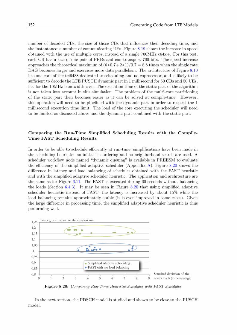
152 Generating Code from LTE Models
number of decoded CBs, the size of those CBs that influences their decoding time, andthe instantaneous number of communicating UEs. Figure 8.19 shows the increase in speedobtained with the use of multiple cores, instead of a single 700MHz c64x+. For this test,each CB has a size of one pair of PRBs and can transport 760 bits. The speed increaseapproaches the theoretical maximum of (6∗0.7+2∗1)/0.7 = 8.8 times when the single rateDAG becomes larger and exercises more data parallelism. The architecture of Figure 8.10has one core of the tci6488 dedicated to scheduling and no coprocessor, and is likely to besufficient to decode the LTE PUSCH dynamic part in 1 millisecond for 50 CBs and 50 UEs,i.e. for the 10MHz bandwidth case. The execution time of the static part of the algorithmis not taken into account in this simulation. The problem of the multi-core partitioningof the static part then becomes easier as it can be solved at compile-time. However,this operation will need to be pipelined with the dynamic part in order to respect the 1millisecond execution time limit. The load of the core executing the scheduler will needto be limited as discussed above and the dynamic part combined with the static part.
Comparing the Run-Time Simplified Scheduling Results with the Compile-Time FAST Scheduling Results
In order to be able to schedule efficiently at run-time, simplifications have been made inthe scheduling heuristic: no initial list ordering and no neighborhood search are used. Ascheduler workflow node named “dynamic queuing” is available in PREESM to evaluatethe efficiency of the simplified adaptive scheduler (Appendix A). Figure 8.20 shows thedifference in latency and load balancing of schedules obtained with the FAST heuristicand with the simplified adaptive scheduler heuristic. The application and architecture arethe same as for Figure 6.11. The FAST is executed during 60 seconds without balancingthe loads (Section 6.4.3). It may be seen in Figure 8.20 that using simplified adaptivescheduler heuristic instead of FAST, the latency is increased by about 15% while theload balancing remains approximately stable (it is even improved in some cases). Giventhe large difference in processing time, the simplified adaptive scheduler heuristic is thusperforming well.
Latency, normalized to the smallest one
Standard deviation of thecore's loads (in percentage)
0,8
0,85
0,9
0,95
1
1,05
1,1
1,15
1,2
1,25
0 1 2 3 4 5 6 7 8 9
Simplified adaptive schedulingFAST with no load balancing
Figure 8.20: Comparing Run-Time Heuristic Schedules with FAST Schedules
In the next section, the PDSCH model is studied and shown to be close to the PUSCHmodel.

PDSCH Model for Adaptive Scheduling 153
8.4 PDSCH Model for Adaptive Scheduling
In the rapid prototyping model of downlink decoding displayed in Figure 7.6, the channelencoding shows many similarities with the uplink channel decoding shown in Figure 7.8.However, the significant difference is that the number of TBs per UE varies between oneand two and must be chosen, and this parameter must be resolved adaptively for each UE.
stat
ic p
art
SDF
Retrieve TBs
PCSDAG
max_CBs_per_TB*nb_TBmax_CBs_per_TB
Not repeated
init subInit
TB Bit Processing Turbo Enc.
(nb_CB);nb_TB;total_TB
Rate Matching Channel Coding Precoding
(code_rate); (modulation); (MU-MIMO_mode)
1(nb_CB)
(nb_CB)
1 1
nb_TB1
1 1
1
max_CBs_per_TB
Figure 8.21: PCSDAG Model of the PDSCH LTE Channel.
PDSCH decoding dominates the LTE downlink decoding. A PDSCH PCSDAG modelfor adaptive scheduling is proposed in Figure 8.21. This model is topologically close tothat of PUSCH, shown in Figure 8.9. Actors from Figure 7.6 have been clustered to reducetheir number. TB bit processing gathers CRC additions and code block segmentations;turbo encoding embeds CB CRC additions; and channel coding contains concatenation,scrambling and constellation mapping. nb TB gives the total number of TBs to encode inthe subframe and (nb CB) the pattern of the number of CBs in each TB.
The maximum graph size is 803 actors. Scheduling this graph adaptively is thusmore costly than scheduling PUSCH and further optimizations of the scheduler will benecessary to minimize this cost. The next section briefly addresses the combination ofuplink decoding, downlink encoding and RACH-PD for entire LTE physical layer executionof an eNodeB.
8.5 Combination of Three Actor-Level LTE Dataflow Graphs
Currently, the majority of signal processing applications have similar structures with threedistinct levels of behavior. Reusing the terminology from Section 4.1.1, these levels are:
� Instruction-level with both control and data streams, efficiently described by imper-ative MoCs and efficiently executed on Von Neumann machines from these descrip-tions.
� Data-dominated actor-level, which is well suited for distributed architectures, pro-vided sufficient data rate is available between operators. Models at this level arecalled concurrency models in the literature.
� Loosely-coupled task-level which is dominated by control streams and is well suitedfor modeling with state machines.
The LTE eNodeB physical layer follows this model structure with three actor-leveltasks: RACH-PD, uplink and downlink which are connected by the control-dominated

154 Generating Code from LTE Models
MAC layer, and contain actors which locally mix control and data dependencies. Theappropriate global execution scheme for the LTE physical layer is certainly a two-levelhierarchical scheduler (Section 8.1.1) with a master/slave task-level scheduler and threeactor-level adaptive schedulers. The technique for task-level scheduling could be based on[HjHL06] where a given task is associated with a particular operator pool depending on its“desire” (the number of operators it reclaims) and the number of available operators. Thejob scheduling algorithm utilized is named Dynamic Equipartitioning (DEQ), and assignsthe same number of operators to each job unless these jobs desire less (the metric is calleddesire). The three actor-level adaptive schedulers then have the goal to use the pool theycontrol for maximum benefit. The next chapter develops the conclusion of the thesis andintroduces possible future work.

CHAPTER 9
Conclusion, Current Status and Future Work
9.1 Conclusion
The most recent algorithms and architectures for embedded systems have become so com-plex that a system-level view of projects from the early design stages to the implemen-tation is now necessary in order to avoid bad design choices and to meet deadlines. Amulti-core DSP implementation of a 3GPP LTE base station is representative of thesenew complex systems which require high optimization. The software of such a hetero-geneous embedded distributed system cannot be efficiently developed without a specialdevelopment chain based on rapid prototyping and system-level simulation. In this the-sis, software rapid prototyping methods were developed to replace certain tediousand sub-optimal steps of the present test-and-refine methodologies for embedded softwaredevelopment. These techniques were applied to the study of a 3GPP LTE base stationphysical layer.
Building a high-level view of a distributed and heterogeneous embedded system bringsnew challenges compared with sequential software development chains. An intimidat-ing number of complex problems arise when algorithm actors are assigned to architectureoperators and algorithm data transfers are assigned to architecture communication nodes.A compromise must be made between model expressivity and power of analysis. Thank-fully, a large amount of relevant literature exists, due to the search for heuristics to solvesimilar parallelization problems such as organizing factories, and projects. In this thesis,heuristics from the literature are presented and enhanced for integration in automaticalprototyping processes for heterogeneous embedded systems.
A system-level view requires new algorithm and architecture models. Whenextracting algorithm parallelism from sequential imperative code, it is tempting to makethe transition between sequential and distributed machines seamless. However, imperativecode introduces useless dependencies to an algorithm and adds a new and unnecessaryparallelism extraction problem to the existing challenges. In this thesis, several dataflowalgorithm models are presented and their use to model LTE is justified and explained.They naturally express algorithm parallelism and have already been intensely studied. Anew simple and expressive System-Level Architecture Model is also introduced, enablinghigh speed simulations.
Programming a distributed embedded system at high-level, designers have several con-

156 Conclusion, Current Status and Future Work
straints to respects and costs to optimize. Moreover, these costs are highly dependenton the system. An embedded software development chain must adapt to these differentcosts and assess the quality of the resulting solutions: it must consist of a framework em-bedding functionalities rather than a monolithic tool. In this thesis, the PREESM rapidprototyping framework was presented. It embeds many functionalities, each with multipleparameters. Importantly, a graphical schedule quality assessment chart was also intro-duced. It displays the parallelism available in an algorithm in terms of latency and showsthe present use of this parallelism in the system.
Finally, code generation from model-based descriptions was explained. LTE physicallayer algorithms were detailed and previously evoked methods were applied to the im-plementation of LTE on multi-core DSPs. These approaches revealed limitations in thecompile-time methods for multi-core scheduling. Depending on the particular algorithmused, the compile-time or the run-time multicore scheduling method should bechosen. The resulting run-time system can be based on different multi-core schedulingstrategies and different execution schemes and must balance the correct use of the parallelarchitecture with the scheduling overhead.
9.2 Current Status
As part of developing new techniques for rapid prototyping and code generation, their be-havior is tested in the PREESM scheduling framework or the multi-core adaptive scheduler.Rapid prototyping with PREESM already offers a user-friendly interface under Eclipse andhas many features explained in this thesis, including control of actor granularity, an op-timization of system latency and load balancing, the support of multiple algorithms andarchitecture topologies, interoperator transfer ordering, static code generation, and so on.The PREESM framework can be found on the Web under Sourceforge. Many configu-rations of LTE have been tested with PREESM and code was implemented and testedfor the RACH-PD with communication libraries developed for TCP on a PC and for thetci6488 processor.
9.3 Future Work
The PREESM scalable scheduler has been designed to enable the comparison and opti-mization of assignment and ordering heuristics separately. Combining existing heuristicsdetailed in the literature and newly developed heuristics, and improving PREESM schedul-ing will allow increasingly complex graphs to be efficiently scheduled.
New applications are currently tested under PREESM including a MPEG4 part 2 intraencoder and decoder. They show limits in the optimality of generated code that alreadyappeared in RACH-PD code generation. These limits will be solved by reducing the inter-core synchronization. Extensions of the algorithm IBSDF model are also tested. Theyenable the modeling of conditions in PREESM and could bring to a coupling of PREESMand the adaptive scheduler.
Certainly the most important future work will be to manage memory during rapid pro-totyping. Memory management should appear in several places in the process. Memory-conscious scheduling can avoid scheduling choices that are impossible to execute becauseof memory size limitations. Memory minimization heuristics have been developed in theliterature to use the same buffers for the storage of several non-overlapping data tokens;these heuristics will be incorporated in the PREESM buffer allocation to reduce the mem-ory needs of the generated code. Memories that are local to operators are often complex

Future Work 157
and cached; the S-LAM model will be extended to include a simple description of theseinternal memories including the cached data accesses.
For adaptive scheduling, scheduler latency and memory footprint can be further re-duced by optimizing the intermediate graph storage, to increase competitiveness for LTEand other applications. Such a scheduler could be adapted to several other problems,including audio and video processing applications with high variability.

158 Conclusion, Current Status and Future Work
APPENDIX A
Available Workflow Nodes in PREESM
The following workflow nodes are shown as they appear in their Graphiti edition. A nodeclass ID identifies its behavior. Each node is provided by the Preesm plug-in precised here.New plug-ins defining new nodes can be programmed. Some port types are known (SDF,architecture, DAG, scenario...) and transfer specific data structures. The port name “xml”is used when xml data files are loaded or stored. This edge does not carry data but onlystates a precedence. Any other type of port can be used for precedence edges.
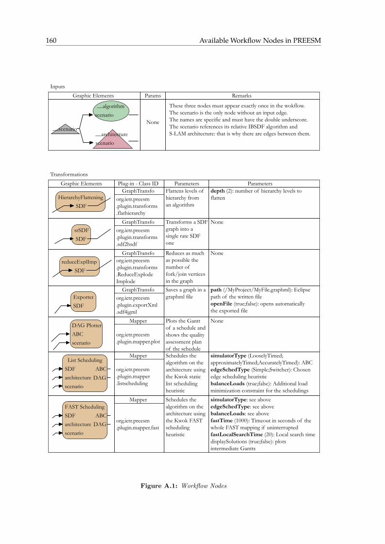
160 Available Workflow Nodes in PREESM
__algorithmscenario
__architecturescenario
__scenario
HierarchyFlatteningSDF
srSDFSDF
reduceExplImplSDF
ExporterSDF
org.ietr.preesm.plugin.transforms.flathierarchy
org.ietr.preesm.plugin.transforms.sdf2hsdf
org.ietr.preesm.plugin.transforms.ReduceExplodeImplode
org.ietr.preesm.plugin.exportXml.sdf4jgml
Graphic Elements Params
None
Remarks
These three nodes must appear exactly once in the wokflow.The scenario is the only node without an input edge.The names are specific and must have the double underscore.The scenario references its relative IBSDF algorithm and S-LAM architecture: that is why there are edges between them.
Graphic Elements Plug-in - Class ID
DAG PlotterABCscenario
org.ietr.preesm.plugin.mapper.plot
GraphTransfo
GraphTransfo
GraphTransfo
GraphTransfo
Mapper
Parametersdepth (2): number of hierarchy levels to flatten
ParametersFlattens levels ofhierarchy froman algorithm
NoneTransforms a SDFgraph into asingle rate SDF one
NoneReduces as muchas possible thenumber offork/join verticesin the graph
path (/MyProject/MyFile.graphml): Eclipsepath of the written fileopenFile (true;false): opens automatically the exported file
Saves a graph in agraphml file
NonePlots the Ganttof a schedule andshows the quality assessment planof the schedule
List SchedulingSDF ABCarchitecturescenario
FAST SchedulingSDF ABCarchitecturescenario
org.ietr.preesm.plugin.mapper.fast
org.ietr.preesm.plugin.mapper.listscheduling
DAG
DAG
Mapper
Mapper
simulatorType (LooselyTimed;approximatelyTimed;AccuratelyTimed): ABCedgeSchedType (Simple;Switcher): Chosen edge scheduling heuristicbalanceLoads (true;false): Additional loadminimization constraint for the schedulings
Schedules thealgorithm on thearchitecture usingthe Kwok static list schedulingheuristic
simulatorType: see aboveedgeSchedType: see abovebalanceLoads: see abovefastTime (1000): Timeout in seconds of thewhole FAST mapping if uninterruptedfastLocalSearchTime (20): Local search timedisplaySolutions (true;false): plotsintermediate Gantts
Schedules thealgorithm on thearchitecture usingthe Kwok FASTschedulingheuristic
Inputs
Transformations
Figure A.1: Workflow Nodes

161
Dynamic queuingSDF ABCarchitecturescenario
Genetic SchedulingSDF ABCarchitecturescenario
PGeneticSDF ABCarchitecturescenario
org.ietr.preesm.plugin.mapper.standardgenetic
org.ietr.preesm.plugin.mapper.pgenetic
org.ietr.preesm.plugin.mapper.DynamicQueuingTransformation
DAGExporterDAG xmlSDFarchitecturescenario
DAG
DAG
DAG
org.ietr.preesm.plugin.mapper.exporter.ImplExportTransform
Mapper
Mapper
Mapper
Mapper
simulatorType: see aboveedgeSchedType: see abovebalanceLoads: see abovefastTime: see abovefastLocalSearchTime: see abovefastNumber: see abovegenerationNumber (100): number of generations before timeoutpopulationSize (100): actors in a population
Schedules thealgorithm on thearchitecture usinga genetic schedulingheuristic
simulatorType: see aboveedgeSchedType: see abovebalanceLoads: see abovefastTime: see abovefastLocalSearchTime: see abovefastNumber: see abovegenerationNumber: see abovepopulationSize: see aboveprocNumber: see above
Schedules thealgorithm on thearchitecture usinga parallel genetic schedulingheuristic
simulatorType: see abovelistType (topological;optimised): Type of listused for scheduling. It can be any topologicallist or one optimized by studying the graphcritical path
Schedules thealgorithm on thearchitecture usingan oblivious listscheduling heuristic
path (/MyProject/MyFile.graphml): Eclipsepath of the written fileopenFile (true;false): opens automatically the exported file
Exports a graphwith scheduleinformation intoa graphml file
org.ietr.preesm.plugin.mapper.scenariogen.ScenarioGenerator
Lua genxml org.ietr.preesm
.XsltTransform
Mapper
Scenario Genxml SDF
architecturescenario
Mapper
inputFile (/MyProject/MyFile.xml): Eclipse path of the xml input fileoutputFile (/MyProject/MyFile.lua): Eclipse path of the output text filexslFile (/MyProject/MyFile.xslt): Eclipse path of the xslt sheet
Transforms a xmlfile into a xml ortext file using a xslt sheet.
dagFile (/MyProject/outDAG.xml): DAG which constraints are importedscenarioFile (/MyProject/in.scenario): scenario initializing all the other parameters
Generates a new scenario from aninput scenarioand the constraints of anexported DAG
PFASTSDF ABCarchitecturescenario
org.ietr.preesm.plugin.mapper.pfastDAG
Mapper simulatorType: see aboveedgeSchedType: see abovebalanceLoads: see abovefastTime: timeout (in s) of one FAST processfastLocalSearchTime: see abovedisplaySolutions: see abovenodesMin (10): Minimum number of actorsassociated to one scheduling coreprocNumber (2): Number of scheduling coresfastNumber (100): Max number of FAST iterations before stopping PFAST
Schedules thealgorithm on thearchitecture usingthe Kwok parallelFAST schedulingheuristic
Transfo Graphic Elements Plug-in - Class ID ParametersParameters
Figure A.2: Workflow Nodes
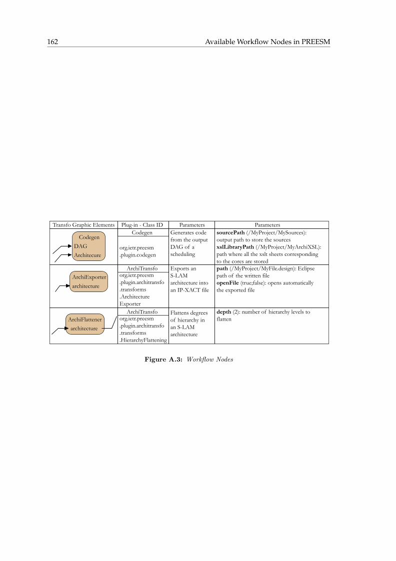
162 Available Workflow Nodes in PREESM
CodegenDAGArchitecure
org.ietr.preesm.plugin.codegen
ArchiExporterarchitecture
ArchiFlattenerarchitecture
Codegen
ArchiTransfo
ArchiTransfoorg.ietr.preesm.plugin.architransfo.transforms.HierarchyFlattening
org.ietr.preesm.plugin.architransfo.transforms.ArchitectureExporter
sourcePath (/MyProject/MySources): output path to store the sourcesxslLibraryPath (/MyProject/MyArchiXSL):path where all the xslt sheets correspondingto the cores are stored
Generates codefrom the outputDAG of a scheduling
path (/MyProject/MyFile.design): Eclipsepath of the written fileopenFile (true;false): opens automatically the exported file
Exports an S-LAM architecture intoan IP-XACT file
depth (2): number of hierarchy levels to flatten
Flattens degreesof hierarchy inan S-LAMarchitecture
Transfo Graphic Elements Plug-in - Class ID ParametersParameters
Figure A.3: Workflow Nodes
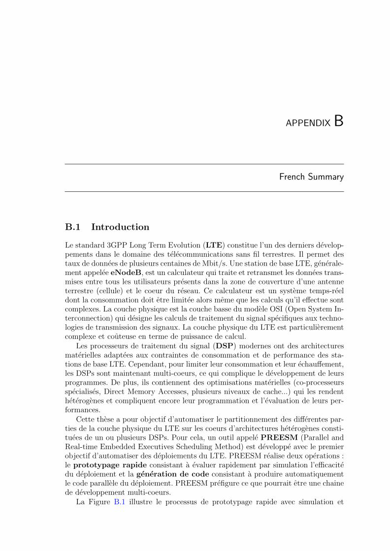
APPENDIX B
French Summary
B.1 Introduction
Le standard 3GPP Long Term Evolution (LTE) constitue l’un des derniers develop-pements dans le domaine des telecommunications sans fil terrestres. Il permet destaux de donnees de plusieurs centaines de Mbit/s. Une station de base LTE, generale-ment appelee eNodeB, est un calculateur qui traite et retransmet les donnees trans-mises entre tous les utilisateurs presents dans la zone de couverture d’une antenneterrestre (cellule) et le coeur du reseau. Ce calculateur est un systeme temps-reeldont la consommation doit etre limitee alors meme que les calculs qu’il effectue sontcomplexes. La couche physique est la couche basse du modele OSI (Open System In-terconnection) qui designe les calculs de traitement du signal specifiques aux techno-logies de transmission des signaux. La couche physique du LTE est particulierementcomplexe et couteuse en terme de puissance de calcul.
Les processeurs de traitement du signal (DSP) modernes ont des architecturesmaterielles adaptees aux contraintes de consommation et de performance des sta-tions de base LTE. Cependant, pour limiter leur consommation et leur echauffement,les DSPs sont maintenant multi-coeurs, ce qui complique le developpement de leursprogrammes. De plus, ils contiennent des optimisations materielles (co-processeursspecialises, Direct Memory Accesses, plusieurs niveaux de cache...) qui les rendentheterogenes et compliquent encore leur programmation et l’evaluation de leurs per-formances.
Cette these a pour objectif d’automatiser le partitionnement des differentes par-ties de la couche physique du LTE sur les coeurs d’architectures heterogenes consti-tuees de un ou plusieurs DSPs. Pour cela, un outil appele PREESM (Parallel andReal-time Embedded Executives Scheduling Method) est developpe avec le premierobjectif d’automatiser des deploiements du LTE. PREESM realise deux operations :le prototypage rapide consistant a evaluer rapidement par simulation l’efficacitedu deploiement et la generation de code consistant a produire automatiquementle code parallele du deploiement. PREESM prefigure ce que pourrait etre une chainede developpement multi-coeurs.
La Figure B.1 illustre le processus de prototypage rapide avec simulation et

164 French Summary
generation de code. Les entrees du processus sont une description des algorithmesdu LTE, une description de l’architecture materielle des DSPs et un scenario four-nissant des informations et des contraintes au prototypage rapide. Les algorithmessont decris en utilisant des graphes flot de donnees qui permettent une extractionefficace du parallelisme qu’ils contiennent. Les elements d’un graphe flot de donneessont appeles acteurs. Les architectures sont decrites en utilisant un nouveau modelegraphique nomme S-LAM pour System-Level Architecture Model. Le coeur du tra-vail de parallelisation consiste a faire des choix de placement et d’ordonnancementdes acteurs de l’algorithme sur les coeurs de l’architecture.
Ce resume est organise a l’image du corps de la these pour pouvoir aisement sereferer au texte integral. La structure de la these est resumee dans la Figure B.1. Unepremiere partie (B.2) traite de l’etat de l’art. Elle se decompose en une explicationdu standard 3GPP LTE, une section traitant des modeles de calculs et en particu-lier des modeles flot de donnees et une section detaillant les techniques existantes deparallelisation de code. La seconde partie (B.3) presente les contributions de cettethese. La Section B.3.1 introduit un modele d’architecture pour le prototypage ra-pide. La Section B.3.2 detaille des methodes permettant d’ameliorer le prototypagerapide et d’evaluer la qualite d’un deploiement. La Section B.3.3 decrit les modelesdu LTE developpes durant cette these ainsi que leur simulation. Enfin, la SectionB.3.4 explique comment generer du code pour executer les differents algorithmes duLTE et la Section B.4 conclut l’etude.
PartitionnementOrdonnancement
Section 2.2: Qu'est-ce qu'un modèle de calculflot de données?
Section 2.3: Quel est l'état de l'artde la parallélisation de code?
Implémentation
Simulation
Section 3.3: Comment modéliser lacouche physique du LTE pour simuler son exécution?
Chapter 3.4: Comment générer du codepour exécuter le LTE sur des DSPs multi-coeurs?
Section 2.1: Commentfonctionne le LTE?
PrototypageRapide
Modèle de la Couche Physique
du LTE
Modèle de DSPMulti-coeurs
Scénario
Section 3.1: Commentmodéliser une architecture?
Section 3.2: Commentpartitionner/ordonnancer?
Partie 2: Etat de l'Art
Partie 3: Contributions
Figure B.1 – Prototypage Rapide et Plan de la These
B.2 Etat de l’Art
B.2.1 Le Standard 3GPP LTE
Contexte de l’Etude
Le 3GPP est l’organisation developpant les standards de telecommunication les plusrepandus sur la planete. La troisieme generation de standards (3G) designe un en-

Etat de l’Art 165
semble de standards successifs apportant chacun une amelioration des performancesdu systeme. L’UMTS (Universal Mobile Telecommunication System) fut le premierstandard de troisieme generation. Deux evolutions de l’UMTS, HSPA (High SpeedPacket Access) et HSPA+, ont augmente la vitesse de transfert de donnees. Le stan-dard LTE est le successeur du HSPA+ et represente une modification profonde dureseau compare a ses predecesseurs. De plus, contrairement a ses prececesseurs, lestandard LTE manipule la voix comme les donnees sous forme de paquets IP (In-ternet Protocol).
Les specifications du systeme LTE etant en pleine evolution, nous considerons lestandard dans sa version 9 finalisee en decembre 2009. Tel qu’illustre par la FigureB.2, cette etude se concentre sur l’implementation de la couche physique du LTEdans les stations de base. La couche physique se compose d’un lien descendant enco-dant le signal a envoyer aux utilisateurs et d’un lien montant decodant le signal recudes utilisateurs. Chaque lien contient une etape de codage canal adaptant le signalbinaire a transmettre aux conditions de transmissions et d’une etape de traitementdes symboles complexes generes par la modulation du signal. Nous ne consideronspas dans cette etude les parties modulation de porteuse et amplification (bloc RFde la figure).
Codage Canal
Lien Descendant du eNodeB
Traitement des symboles
Décodage Canal
Lien Montant du eNodeB
bits symboles (valeurs complexes)
symboles (valeurs complexes)
bits symboles (valeurs complexes)
symboles (valeurs complexes)
Couche 2 OSI
Traitement de la Couche Physique en Bande de Base
contrôledonnées
Paquet IP
Paquet IP
RF
RFCouche 2 OSI Traitement des symboles
Figure B.2 – Objets de l’Etude du LTE
Objectifs du LTE
Compare aux precedents standards, le LTE a de tres fortes contraintes de perfor-mance :
� Des taux de transfert sans precedent. Le lien descendant supporte 100Mbit/s en supposant des recepteurs a deux antennes et le lien montant 50Mbit/s.
� Une latence reduite a 10 millisecondes pour la reponse a un message.
� Un cout par bit reduit par une meilleure utilisation de la bande de frequenceallouee.
� Une flexibilite du spectre avec la possibilite de deployer un lien montantet un lien descendant chacun sur des bandes de frequences de largeurs pa-rametrables entre 1.4 MHz et 20 MHz.

166 French Summary
� Une consommation reduite des terminaux en deportant autant que pos-sible la complexite des calculs dans la station de base.
� Une architecture du reseau simplifiee. Cette architecture, nommee SystemArchitecture Evolution (SAE) redefinit a la fois la partie acces radio et la partiecoeur du reseau.
� Le transport efficace a la fois de la voix et des donnees, le tout enutilisant la technologie IP (Internet Protocol).
� Des cellules de taille tres variables, couvrant de quelques metres (femto-cells) a 115 km (macrocells) pour s’adapter aux densites de population locales.
� La connectivite d’utilisateurs a grande vitesse. Un utilisateur devantpouvoir rester connecte meme s’il voyage a 350 km/h.
� La gestion de communications simultanees avec de nombreux utili-sateurs (200 a 400 selon la largeur de bande).
Ces contraintes ont necessite l’utilisation de techniques complexes a la fois pourles deux liens montant et descendant. Ces techniques rendent la couche physique duLTE complexe et couteuse.
Technologies de la Couche Physique du LTE
Les liens montant et descendant sont tous deux a large bande. Le spectre de chaquelien est divise en sous-porteuses transportant des composantes differentes du fluxde donnees. Le lien descendant utilise une technologie nommee OFDMA (Ortho-gonal Frequency Division Multiplexing Access) qui optimise les debits de donneesalors que le lien montant utilise la technologie SC-FDMA (Single Carrier-FrequencyDivision Multiplexing Access) qui offre un bon compromis entre debit et consomma-tion electrique de l’amplificateur de puissance de l’utilisateur. La reduction de cetteconsommation est primordiale car les utilisateurs ont le plus souvent un terminalalimente par batterie. Les techniques OFDMA et SC-FDMA utilisent une estimationprecise de la qualite instantanee du canal de transmission. Elles sont combinees avecde multiples antennes d’emission et de reception permettant des debits plus elevesgrace au multiplexage spatial, souvent appele effet MIMO (Multiple Input MultipleOutput).
Une procedure nommee “Random Access Procedure” permet a de nouveaux uti-lisateurs de se connecter a une station de base. Ils envoient pour cela une signaturedans une zone temps/frequence preallouee. Le processus de detection des signaturesenvoyees s’appelle la detection de preambules. Cette detection est couteuse en termede calculs et son comportement est different de ceux des liens montant et descendant.La detection de preambules sera modelisee a part dans la Section B.3.3.
B.2.2 Les Modeles Flot de Donnees
Les modeles flot de donnees ont prouve leur efficacite pour la modelisation d’ap-plications paralleles avec dependances de donnees. Ils representent les applicationspar des graphes dont les noeuds (ou acteurs) sont des entites de code sequentiel et

Etat de l’Art 167
les arcs representent des donnees circulant entre les acteurs. La Figure B.3 illustrequelques modeles flot de donnees. Chaque modele est un compromis entre expressi-vite et analysabilite. L’expressivite determine quels algorithmes seront modelisablesalors que l’analysabilite determine quelles informations sur le comportement du codepourront etre extraites durant la phase de compilation. Une grande analysabilite estnecessaire pour pouvoir partitionner au moment de la compilation les differentes par-ties de l’algorithme. Un modele Turing complet permet de representer un algorithmequelconque. La compacite du modele varie egalement, i.e. sa capacite a representerun algorithme avec peu d’elements.
KPNIDFBDF
PSDF
CSDFSDF
DAG
srSDF srDAG
...
Exp
ress
ivité
Analysabilité
ModèlesTuring complets
Modèlesnon Turing complets
DFDDFKPNIDFBDFSDFPSDFIBSDF CSDFsrSDF DAG srDAG
Data FlowDynamic DFKahn Process NetworkInteger DFBoolean DFSynchronous DFParameterized SDFInterface-Based Hierarchical SDFCyclo Static DFsingle rate SDFDirected Acyclic Graphsingle rate DAG
DDF
Modèles principaux Modèles dérivés Réseaux de Processus Flot de Données
IBSDF
Figure B.3 – Modeles de Calcul Flot de Donnees
Les modeles que nous utilisons pour representer le LTE sont une version modifieedu SDF (Synchronous Dataflow) nommee IBSDF (Interface-Based Hierarchical Syn-chronous Dataflow) et une version modifiee du PSDF (Parameterized SynchronousDataflow) nommee PCSDAG (Parameterized Cyclo Static Directed Acyclic). Le SDFet le PSDF sont des modeles de la litterature frequemment utilises. Le IBSDF est unmodele ajoutant au SDF une hierarchie controlee par l’utilisateur pour simplifier ladescription des algorithmes. Le PCSDAG est un modele a la fois rapide a analyseret suffisamment expressif pour modeliser les algorithmes tres variables du LTE.
B.2.3 Le Prototypage Rapide et la Programmation des ArchitecturesMulticoeurs
La programmation d’architectures multi-coeurs a donne lieu a de nombreux tra-vaux de recherche conduisant a des resultats tres differents dependant des objectifset contraintes de l’etude (programmation generique a tous type d’applications ouspecifique au traitement du signal, architectures homogenes ou heterogenes, memoirepartagee ou distribuee, minimisation de la latence ou du debit de donnees traitees...).Nous nous interessons particulierement ici aux applications de traitement du signaldont la couche physique du LTE fait partie. Les architectures cible sont heterogenesa memoire distribuee ou partagee et nous minimisons principalement la latenced’execution car elle est la principale contrainte de la couche physique du standardLTE.
Nous pouvons distinguer trois niveaux de parallelisme : le niveau instruction, leniveau thread et le niveau tache. Le parallelisme de grain moyen (niveau thread ouacteur dans le cadre du flot de donnees) est le parallelisme le moins traite dans la

168 French Summary
litterature et le plus utile pour minimiser la latence de la couche physique du LTEsur architecture distribuee. Cette these a donc pour objectif le parallelisme a grainmoyen.
Acteur1 Acteur2Acteur3 Acteur4
Coeur1 Coeur2 Coeur1 Coeur2Coeur1 Coeur2
Acteur1 Acteur2Acteur3 Acteur4
Acteur1 Acteur2Acteur3 Acteur4
Sources Temps
3 2
14
21
12
Régions Parallèles
Chronom
étrage
Extraction
Partitionnement
Ordonnancem
ent
Figure B.4 – Les quatre phases de la parallelisation a grain moyen : extraction, partitionnement,ordonnancement et chronometrage
La parallelisation d’un code a grain moyen consiste en quatre etapes (FigureB.4) :
� L’ extraction consiste a extraire le zones potentiellement paralleles (acteurdans le cadre du flot de donnees) du code source.
� Le partitionnement consiste a choisir un coeur/coprocesseur pour executerchaque acteur.
� L’ ordonnancement consiste a ordonner l’execution des acteurs assignes a unmeme coeur/coprocesseur.
� Le chronometrage consiste a choisir le moment ou chaque acteur est execute.
Dans le domaine que nous etudions ici, les systemes embarques, [POH09] dis-tingue quatre classes de methodes pour effectuer une parallelisation a grain moyen :
� Les methodes basees sur la compilation consistent a extraire le zonesparalleles d’un code sequentiel par des methodes de compilation.
� Les extensions de langage consistent a laisser le developpeur ajouter des ins-tructions specifiques a un code sequentiel pour preciser comment le paralleliser.
� La methode basee sur la plateforme se refere a une technique particulierede l’auteur.
� Les methodes basees sur les modeles flot de donnees consistent a decrirele comportement general des algorithmes avec un modele simple a etudier pourla parallelisation.
Les methodes flot de donnees ont l’avantage de supprimer l’etape d’extractionpuisque les modeles sont concus pour exprimer naturellement le parallelisme. Nouschoisissons de resoudre le probleme de l’execution parallele du LTE en developpantl’outil PREESM base sur les modeles flot de donnees. Cet outil est developpe dansde cadre de la these en collaboration avec Texas Instruments. Le developpement del’outil est partage avec deux autres doctorants : Jonathan Piat et Matthieu Wipliez.L’outil est open source et disponible sur internet. Il automatise la phase de parti-tionnement et genere un code dit “self-timed”, c’est a dire partitionne et ordonnance

Contributions 169
a la compilation (partitionnement statique) tout en laissant le systeme d’executionfaire la phase de chronometrage.
Le partitionnement statique est illustre par la Figure B.5. Le graphe d’algorithmecontient cinq acteurs a ,b ,c ,d et e et des arcs symbolisant le transfert de donneesentre acteurs. Le graphe d’architecture contient trois coeurs et un DMA (DirectMemory Access) qui se charge de piloter leurs transferts. Le scenario contient destemps typiques d’execution pour chaque acteur sur chaque type de coeur. A par-tir de ces informations, le partitionneur choisis partitionnement, ordonnancementet chronometrage et simule l’execution en l’affichant dans un graphique de Gantt.L’etape de chronometrage n’est pas transmise a la phase d’execution. Les problemesde partitionnement et ordonnancement pour minimiser la latence sont NP-complets :il est donc necessaire de trouver des heuristiques pour les resoudre.
aDSP1DSP2DSP3
b
c
d
e
3 octets
a bc
d
e
0 10 20
Temps de réponse = 16
PE1
DMA2
PE2
PE3
vitesse=1type=defP
type=defP
type=defP2 octets
3 octets
2 octets
CN1
CN1
(b,defP=8))(a,defP=3))
(d,defP=5))(c,defP=5))
(e,defP=5))
byte=1unité mem.
AlgorithmeArchitecture
Scénario Déploiement
Figure B.5 – Partitionnement multi-coeurs a partir d’un modele flot de donnees de l’algorithmeet d’un graphe d’architecture
De tres nombreuses heuristiques ont ete inventees pour resoudre le problemede partitionnement et ordonnancement. [Kwo97] reference et evalue de nombreusesmethodes avant d’en proposer trois nouvelles : une methode gloutonne, une methodenommee FAST utilisant des sauts probabilistes et un algorithme genetique. Ces troisalgorithmes ont ete implementes dans l’outil PREESM et la methode gloutonne estutilisee dans un partitionneur adaptatif presente Section B.3.4.
Les quatre prochaines sections detaillent les contributions de cette these.
B.3 Contributions
B.3.1 Un Modele d’Architecture pour le Prototypage Rapide
Le modele d’architecture S-LAM (System-Level Architecture Model) est unnouveau modele permettant de decrire simplement des comportements complexes.La Figure B.6 montre les differents elements constituant le modele. L’element prin-cipal est l’operateur qui represente un calculateur sequentiel capable d’executer desacteurs. Les liens de donnees, orientes ou non, relient les operateurs a des noeudsde communication. Les noeuds de communication permettent des interconnexionsmulti-points de liens de donnees. Il en existe deux types :
� Les noeuds de competition prennent en compte la competition des differentstransferts qui transitent par eux.
� Les noeuds paralleles, a l’inverse, peuvent faire transiter simultanement plu-sieurs transferts entre plusieurs paires d’operateurs.

170 French Summary
Utiliser un lien de competition ajoute un cout a la simulation d’un deploiementsur cette architecture car il faut ordonnancer les transferts sur ce noeud. Le developpeurpeut donc regler la complexite de simulation de son modele en placant des noeudsde competition sur les liens susceptibles de limiter la performance du systeme.
Lien de Contrôle
Lien de setup
Liens de Données
Lien non Orienté Lien Orienté
Element de Calcul
Opérateur
Noeuds de Communication
Noeud de CompétitionNoeud Parallèle
Médiateurs de Communication
RAM DMA
Figure B.6 – Elements du modele d’architecture S-LAM
La RAM (Random Access Memory) est une memoire que peuvent se partagerplusieurs operateurs. Si le chemin entre deux operateurs contient une RAM, ils com-muniquent en se partageant une memoire ; sinon, il s’envoient des messages. Le DMA(Direct Memory Access) est un gestionnaire de transferts qui permet a un operateurd’effectuer des calculs en parallele avec ses propres transferts. Le lien de “setup”permet de preciser quel operateur peut programmer quel DMA et combien de tempsest necessaire pour cette programmation.
GEM1
GEM2
GEM3
EDMA3
2700 cycles
2700 cycles
2700 cycles
SCR
2 Goctets/s
VCP2 TCP2
RIO
0.125 Goctets/s
VCP2TCP2
EDMA3
2700 cycles
2700 cycles
2700 cycles
2 Goctets/s
SCR
GEM1
GEM2
GEM3
Figure B.7 – Exemple d’un modele S-LAM : deux DSPs TMS320TCI6488
La Figure B.7 montre un exemple de description S-LAM. Deux processeurs detype TMS320TCI6488 sont connectes par un lien de type RapidIO de vitesse 1 Gbits/s. Chaque processeur contient trois coeurs (GEM) de type c64x+. Les commu-nications locales des processeurs se font via un lien parallele nomme SCR (SwitchedCentral Resource) de vitesse 2 G octets/s. Des coprocesseurs permettent d’accelererles encodage/decodage Viterbi (VCP2) et turbo (TCP2). Tous les transferts, y com-pris entre processeurs, sont pilotes par les DMAs dont le demarrage necessite 2700cycles. Ce modele simple decrit precisement le comportement reel de l’architecture.
A partir du modele S-LAM, un routage est calcule et permet d’accelerer la si-mulation de l’architecture. Chaque paire d’operateurs est alors associee au meilleurlien qui les relie et ce lien est utilise pour le prototypage rapide. Le resultat est unmodele expressif, simple et rapide a simuler.

Contributions 171
B.3.2 Amelioration du Prototypage Rapide
De nouvelles methodes de prototypage rapide sont introduites dans l’outil PREESM.Elles ameliorent la flexibilite, les performances et l’ergonomie de l’outil de partition-nement automatique. Une premiere methode est l’utilisation du scenario et du“workflow”. Le scenario contient les informations liees a la fois a l’algorithme et al’architecture. Il est stocke au format XML dans PREESM et permet de reutilisertout algorithme avec toute architecture. Un “workflow” est un graphe decrivantl’enchaınement des transformations appliquees aux entrees du prototypage rapide.Le workflow de la Figure B.8 applique trois transformations a l’algorithme d’entree(flattening, srSDF et reduceForkJoin), puis partitionne l’algorithme pour l’architec-ture (scheduling), genere un code “self-timed” et affiche le diagramme de Gantt dudeploiement. Ce workflow peut etre execute dans l’outil PREESM, qui applique alorsles transformations specifiees sur les modeles d’entree.
SchedulingSDF ABC
architecturescenario
DAG
__algorithmscenario
__architecturescenario
__scenario
FlatteningSDF
srSDFSDF
DAG PlotterABCscenario
depth=2
reduceForkJoinSDF
CodegenDAGArchitecture
Figure B.8 – Exemple d’un “workflow” rendant flexible le prototypage rapide
Le partitionnement est calcule par un partitionneur composite dont la struc-ture est illustree Figure B.9. Une partie calcule les choix de partitionnement pen-dant que l’autre, nommee ABC (Architecture Benchmark Computer), calcule le coutdes deploiements obtenus. Plusieurs implementations sont disponibles pour les deuxparties, permettant un choix dans la complexite et la precision du partitionneur. Deplus, le cout retourne par l’ABC etant abstrait, il peut representer indifferemmentune latence, un cout memoire, une consommation d’energie ou un cout composite.Cette structure permet de minimiser simplement differents criteres.
Partitionnementd'acteurs
Architecture Benchmark
Computer (ABC)
Nombre d'opérateurs
Partitionnement
Coût du déploiement
Partitionneur
Algorithme S-LAM Scénario
Figure B.9 – Structure interne d’un partitionneur flexible
Un exemple de cout composite est l’equilibrage des charges de calcul entreles operateurs. Cet equilibrage est positif pour la consommation electrique du cir-cuit. Il est naturel lorsque l’on minimise la latence, dans l’hypothese (imaginaire)d’une architecture a une infinite d’operateurs avec des liens infiniment rapides. Le

172 French Summary
nombre limite d’operateurs, leur caractere heterogene, ainsi que les liens de donneeslimites rendent differents les deux criteres latence et equilibrage des charges. Unesolution efficace est d’utiliser un ABC retournant un cout composite : la sommede la latence et de l’ecart type des charges. La Figure B.10 montre le resultat decette modification de cout sur un exemple d’application du LTE. Les charges sontsensiblement equilibrees et la latence n’est pas sensiblement deterioree.
0,8
0,85
0,9
0,95
1
1,05
1,1
1,15
1,2
1,25
0 1 2 3 4 5 6 7 8 9
Egalisation des chargesPas d'égalisation des charges
Latence, normalisée à la plus courte
Ecart type des charges des coeurs (en pourcentage)
Figure B.10 – Equilibrage des charges de calculs entre les differents operateurs
Dans le cas le plus courant ou la minimisation de la latence d’execution estl’objectif principal du partitionnement, la qualite d’un deploiement peut etre evalueepar le “speedup”. Le speedup correspond a l’acceleration du calcul due a l’utilisationd’une architecture distribuee. Il est egal au temps d’execution sur un operateur divisepar le temps d’execution sur l’architecture distribuee. Ce speedup peut etre affiche,pour une architecture homogene, sur un graphique illustre Figure B.11. Le graphiquede la partie droite permet d’evaluer le deploiement situe en bas a gauche de la figure.L’algorithme etudie est place en haut a gauche de la figure. Le travail corresponda la somme des temps d’execution des acteurs et le chemin critique est le plus longchemin entre un acteur entrant et un acteur sortant. Sur ce graphique, genere apartir du modele d’algorithme, le point correspond au deploiement que l’on veutevaluer. Le speedup est donne en ordonnee et le nombre d’operateurs homogenes enabscisse. Trois courbes circonscrivent une zone correspondant aux deploiements debonne qualite :
� La courbe Ssupworksignifie que le speedup ne peut pas etre superieur au nombre
d’operateurs
� La courbe Ssupspan signifie que l’algorithme a une limite en terme de parallelisme
� La courbe SinfGSTest donnee par le “Greedy Scheduling Theorem” (GST). Ce
theoreme fixe un minimum de parallelisme que tout algorithme glouton peutatteindre a partir d’un algorithme donne. Un deploiement sous cette limitesignifie que les efforts de partitionnement intelligent a la compilation n’ontpas conduit a un resultat satisfaisant. Plusieurs raisons peuvent expliquer desperformances inferieures a la limite GST : un lien de donnees trop lent entreles operateurs ou de mauvais choix de partitionnement/ordonnancement.
Moyennant quelques precautions, l’affichage du speedup peut egalement etre uti-lise pour des architectures heterogenes. Cet affichage permet d’evaluer rapidement
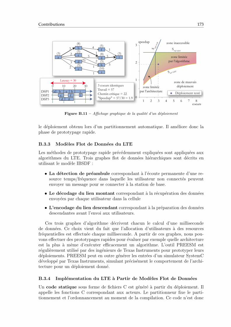
Contributions 173
a
DSP1DSP2DSP3
5
1
5
5
4
1
2
1
b
c
d
e
f
g
h
j
(8)
(5)
(5)(5)
3
2
32
(3)
(5)
(8)
(5)
(3)
a bcd
ef
g
h i
0 10 20 30
Latency = 303 coeurs identiquesTravail = 57Chemin critique = 22"Speedup" = 57/30 = 1.9
i(10)
1
j0
1
2
3
1 2 3 4 5 6 7 8
Déploiement testé
zone limitéepar l’architecture
zone limitéepar l’algorithme
zone de mauvaisdéploiement
zone inaccessible
S sup
work
Ssup span
S inf GST
coeurs
speedup
Figure B.11 – Affichage graphique de la qualite d’un deploiement
le deploiement obtenu lors d’un partitionnement automatique. Il ameliore donc laphase de prototypage rapide.
B.3.3 Modeles Flot de Donnees du LTE
Les methodes de prototypage rapide precedemment expliquees sont appliquees auxalgorithmes du LTE. Trois graphes flot de donnees hierarchiques sont decrits enutilisant le modele IBSDF :
� La detection de preambule correspondant a l’ecoute permanente d’une re-source temps/frequence dans laquelle les utilisateur non connectes peuventenvoyer un message pour se connecter a la station de base.
� Le decodage du lien montant correspondant a la recuperation des donneesenvoyees par chaque utilisateur dans la cellule
� L’encodage du lien descendant correspondant a la preparation des donneesdescendantes avant l’envoi aux utilisateurs.
Ces trois graphes d’algorithme decrivent chacun le calcul d’une millisecondede donnees. Ce choix vient du fait que l’allocation d’utilisateurs a des resourcesfrequentielles est effectuee chaque milliseconde. A partir de ces graphes, nous pou-vons effectuer des prototypages rapides pour evaluer par exemple quelle architectureest la plus a meme d’executer efficacement un algorithme. L’outil PREESM estregulierement utilise par des ingenieurs de Texas Instruments pour prototyper leursdeploiements. PREESM peut en outre generer les entrees d’un simulateur SystemCdeveloppe par Texas Instruments, simulant precisement le comportement de l’archi-tecture pour un deploiement donne.
B.3.4 Implementation du LTE a Partir de Modeles Flot de Donnees
Un code statique sous forme de fichiers C est genere a partir du deploiement. Ilappelle les fonctions C correspondant aux acteurs. Le partitionneur fixe le parti-tionnement et l’ordonnancement au moment de la compilation. Ce code n’est donc
174 French Summary
adapte qu’a des algorithmes dont le comportement est relativement stable dans letemps. C’est le cas de la detection de preambule qui correspond a une ecoute per-manente et stable d’eventuels messages. La procedure de generation de code dansPREESM est illustree dans la Figure B.12. Le partitionneur calcule le deploiementen utilisant le graphe S-LAM de l’architecture, le graphe IBSDF de l’algorithme etun scenario. Un code generique au format XML est ensuite genere. Des fichiers IDL(Interface Description Language) donnent le prototype de chaque fonction appeleepar la generation de code. Une transformation XSL transforme le code generiqueXML en un code C ayant la bonne syntaxe pour l’operateur cible. Finalement, lecompilateur genere un executable par operateur en utilisant des bibliotheques detransfert ainsi que le code des acteurs. Cette methode de generation de code estappliquee a la detection de preambule. Le decodage du lien montant et l’encodagedu lien descendant necessitent de prendre en compte leur grande variabilite.
op2
DMA
op3
op1
modèle S-LAM du tci8488avec des operateurs
de type c64x+ Partitionneur
Génération de C
ode
Transformation X
SL
Com
pilateur TI
bibliothèques de communicationet code des acteurs
op1.xml op1.c op1.exe
op3.xml op3.c op3.exe
op2.xml op2.c op2.exe
prototypes IDL
Déploiem
ent
Algorithmeet scenario c64x+.xsl
Figure B.12 – Generation de code “self-timed” a partir du deploiement statique
Chaque milliseconde, la station de base echange des donnees avec ses utilisateursconnectes. Les donnees sont rassemblees en “Code Blocks” (CB) de taille variable. Letype de cellule le plus evolue peut allouer simultanement 100 CBs a jusqu’a une cen-taine d’utilisateurs. La Figure B.13 illustre le nombre d’allocations possibles lorsquel’on alloue N CBs a des utilisateurs. Le nombre d’allocations possibles augmenteexponentiellement avec le nombre de CBs alloues : il atteint presque 200 millionspour 100 CBs. La taille variable des CBs ainsi que leur nombre egalement variableaugmente encore considerablement le nombre de possibilites de configurations. Laconfiguration des graphes du decodage du lien montant et de l’encodage du liendescendant depend de ces allocations et ces algorithmes extremement variables sepretent mal au partitionnement statique.
Une solution au partitionnement du decodage du lien montant et de l’encodage dulien descendant est de partitionner durant l’execution, alors que tous les parametresinstantanes du graphe sont connus. Il faut alors quitter le schema d’execution decentra-lise utilise dans la generation de code statique et utiliser a la place un schemad’execution maıtre/esclave (Figure B.14). Dans le schema d’execution decentralise,tous les operateurs sont equivalents et executent les acteurs qui leur sont assignesstatiquement. Les acteurs s’executent des que leurs donnees d’entree sont dispo-nibles. Dans le schema d’execution maıtre/esclave, un operateur maıtre dirige lesoperations et assigne dynamiquement les acteurs a des operateurs esclaves. Pour cenouveau schema d’execution, il faut concevoir le code de controle dont l’elementprincipal est un partitionneur adaptatif.

Contributions 175
3 CBs2 CBs
5 CBs4 CBs
7 CBs
6 CBs
8 CBs
1 CB 1 motif d'allocation; 1 utilisateur max
3 motifs d'allocation; 3 utilisateurs max
7 motifs d'allocation; 5 utilisateurs max11 motifs d'allocation; 6 utilisateurs max
15 motifs d'allocation; 7 utilisateurs max
22 motifs d'allocation; 8 utilisateurs max
100 CBs50 CBs25 CBs 1958 motifs d'allocation; 25 utilisateurs max
204226 motifs d'allocation; 50 utilisateurs max190569292 motifs d'allocation; 100 utilisateurs max
CB par utilisateur
utilisateurs
2 motifs d'allocation; 2 utilisateurs max
5 motifs d'allocation; 4 utilisateurs max
...
Figure B.13 – Diagrammes de Ferrer : les differentes allocations possible de N CBs a des utili-sateurs
controlcode
master task
slave task
Actor A
slave task
Actor Bslave task
Actor DActor C
assigns
assigns
assigns
finished
(a) Schema d’Execution Maıtre/Esclave
opérateur
Acteur A
opérateur
Acteur D
Acteur Copérateur
Acteur B
lance lance
lance
(b) Schema d’Execution Decentralise
Figure B.14 – Schemas d’Execution
La Figure B.15 illustre la structure d’un partitionneur adaptatif base sur unmodele flot de donnees. Une phase d’initialisation executee au demarrage genereun graphe parametre de type PCSDAG qui represente le comportement global del’algorithme. A partir de ce graphe de reference et des parametres instantanes, ungraphe de type single rate DAG est genere chaque milliseconde durant une phased’expansion du graphe. Ce graphe genere represente l’execution d’une instance dugraphe incluant les instances des acteurs et les transferts de donnees. Une phasede partitionnement choisit ensuite le partitionnement de chaque acteur. Les deuxoperations expansion et partitionnement doivent etre extremement efficace pour etreexecutees dans tous les cas en moins d’une milliseconde, c’est a dire le temps separantdeux choix d’allocation differents.
Les performances du partitionneur adaptatif developpe durant cette these sontillustrees Figure B.16. Ce partitionneur permet de deployer en temps reel le decodagedes donnees du lien montant a condition que le nombre d’operateurs esclaves soitinferieur a 8. Un tel partitionneur ouvre de nouvelles perspectives pour la pa-rallelisation d’algorithmes extremement variables tels que le decodage du lien mon-tant et l’encodage du lien descendant dans les stations de base LTE.

176 French Summary
Expansiondu Graphe
PartitionnementGlouton
Initialisation
LTE Couche OSI 2
PCSDAGsrDAG Déploiement
vers le système d'exécution
paramètres du PCSDAGPartitionneur Adaptatif
< 1ms
architecture
Figure B.15 – Structure interne du partitionneur adaptatif
TotalExpansion du graphePartitionnement glouton
Temps en cycles
Nombre de coeurs/coprocesseurs dans l’architecture
01000002000003000004000005000006000007000008000009000001000000
0 1 2 3 4 5 6 7 8
Figure B.16 – Temps d’execution pire cas du partitionneur adaptatif applique au decodage desdonnees du lien montant en fonction du nombre d’operateurs esclaves
B.4 Conclusion
Les solutions logicielles et materielles des systemes embarques modernes sont deve-nues tellement complexes qu’une etude au niveau systeme est maintenant necessairepour eviter les mauvais choix de conception et respecter les contraintes. L’implemen-tation sur DSP multi-coeurs du traitement du signal des stations de base 3GPP LTEest un exemple de ces systemes complexes. Durant cette these, des methodes de pro-totypage rapide utilisant les modeles flot de donnees ont ete mises en place. Ellespermettent de simuler le deploiement d’un algorithme sur une architecture distribueeet de generer un code efficace.
Les contributions de cette these sont de plusieurs types. Un nouveau modeled’architecture est introduit. Il est simple, expressif, et permet une simulation rapidede l’architecture decrite. Un nouvel outil nomme PREESM pour le prototypagerapide est presente. Une nouvelle structure interne pour le partitionneur, c’est adire le coeur du prototypage rapide sur architecture distribuee, est introduite etexpliquee. Elle rend le processus adaptable et permet de minimiser plusieurs typesde fonction de cout pendant le partitionnement. Un exemple de fonction de coutest donne ; il permet d’egaliser efficacement les charges de calcul sur les differentsoperateurs, ce qui a generalement un effet positif sur la consommation electriquedu systeme. De nombreux modeles de calcul sont expliques et le choix de modelespour decrire la couche physique du 3GPP LTE est justifie. Le fonctionnement etl’agencement des algorithmes du LTE sont detailles ainsi que des methodes poursimuler l’execution et generer le code. Lorsque cela est possible, par exemple pour

Conclusion 177
la detection de preambule, le partitionnement statique conduit a une generation decode qui ne remet pas en cause le partitionnement des acteurs. Dans les cas pluscomplexes, par exemple les liens montant et descendant, un partitionnement en-ligneest calcule. Le partitionneur adaptatif en-ligne est temps reel sur les liens montant etdescendant et constitue donc une solution possible a leur implementation parallele.

178 French Summary

List of Figures
1.1 Comparing a Present Single-core Development Chain to a Possible Devel-opment Chain for Multi-core DSPs . . . . . . . . . . . . . . . . . . . . . . . 5
1.2 Rapid Prototyping and Thesis Outline . . . . . . . . . . . . . . . . . . . . . 8
2.1 3GPP Standard Generations . . . . . . . . . . . . . . . . . . . . . . . . . . 11
2.2 A three-sectored cell . . . . . . . . . . . . . . . . . . . . . . . . . . . . . . . 12
2.3 Scope of the LTE Study . . . . . . . . . . . . . . . . . . . . . . . . . . . . . 14
2.4 LTE Systeme Architecture Evolution . . . . . . . . . . . . . . . . . . . . . . 15
2.5 Protocol Layers of LTE Radio Link . . . . . . . . . . . . . . . . . . . . . . . 16
2.6 Data Blocks Segmentation and Concatenation . . . . . . . . . . . . . . . . . 17
2.7 Radio Propagation, Channel Response and Reciprocity Property . . . . . . 19
2.8 Uplink and Downlink Data Processing in the LTE eNodeB . . . . . . . . . . 22
2.9 LTE downlink and uplink multiplexing technologies . . . . . . . . . . . . . . 22
2.10 Comparison of OFDMA and SC-FDMA . . . . . . . . . . . . . . . . . . . . 23
2.11 Cyclic Prefix Insertion . . . . . . . . . . . . . . . . . . . . . . . . . . . . . . 24
2.12 LTE Time Units . . . . . . . . . . . . . . . . . . . . . . . . . . . . . . . . . 25
2.13 Different types of LTE duplex modes . . . . . . . . . . . . . . . . . . . . . . 26
2.14 LTE Link Adaptation . . . . . . . . . . . . . . . . . . . . . . . . . . . . . . 27
2.15 LTE Forward Error Correction methods . . . . . . . . . . . . . . . . . . . . 28
2.16 LTE link adaptation . . . . . . . . . . . . . . . . . . . . . . . . . . . . . . . 30
2.17 Reference Signals location in the uplink resources . . . . . . . . . . . . . . . 31
2.18 Uplink Channels . . . . . . . . . . . . . . . . . . . . . . . . . . . . . . . . . 32
2.19 Length-63 Zadoff-Chu Sequences with index 25, 29 and 34 . . . . . . . . . 33
2.20 Contention-Based Random Access Procedure. . . . . . . . . . . . . . . . . . 36
2.21 Baseband Spectrum of a Fully-Loaded 20 MHz LTE Downlink . . . . . . . 37
2.22 Downlink multiple user scheduling and reference signals . . . . . . . . . . . 38
2.23 Gold Pseudo Random Sequence Generation . . . . . . . . . . . . . . . . . . 40
2.24 Layer Mapping and Precoding for Spatial Diversity with Different Multi-antenna Parameters . . . . . . . . . . . . . . . . . . . . . . . . . . . . . . . 41
2.25 Layer Mapping and Precoding for Spatial Multiplexing with different mul-tiantenna parameters . . . . . . . . . . . . . . . . . . . . . . . . . . . . . . . 42
2.26 Downlink PSS, SSS, RS and PBCH localization in subframes. . . . . . . . . 43
3.1 Main Types of Process Network Model of Computation . . . . . . . . . . . 47
179

180 List of Figures
3.2 A Few Dataflow MoC Graph Examples . . . . . . . . . . . . . . . . . . . . . 49
3.3 The Topology Matrix and Repetition Vector of an SDF Graph . . . . . . . 51
3.4 SDF Graph and its Acyclic Precedence Expansion Graph . . . . . . . . . . 53
3.5 The Topology Matrix and Repetition Vector of a CSDF Graph . . . . . . . 55
3.6 Illustrating Compactness of CSDF Model Compared to SDF . . . . . . . . . 55
3.7 PSDF Example . . . . . . . . . . . . . . . . . . . . . . . . . . . . . . . . . . 56
3.8 Comparing Direct Hierarchical SDF with IBSDF . . . . . . . . . . . . . . . 57
3.9 IBSDF Sub-Graph Example and Its Single Rate Equivalent . . . . . . . . . 58
4.1 The Von Neumann Architecture of an Operator . . . . . . . . . . . . . . . . 64
4.2 The Four Phases of Middle-Grain Parallelization: Extraction, Assignment,Ordering and Timing . . . . . . . . . . . . . . . . . . . . . . . . . . . . . . . 66
4.3 Example of a schedule Gantt chart . . . . . . . . . . . . . . . . . . . . . . . 70
4.4 T-Level and B-Level of a Timed Directed Acyclic Graph . . . . . . . . . . . 71
4.5 Construction of an Actor List in Topological Order . . . . . . . . . . . . . . 72
4.6 Genetic Algorithm Atomic Operations: Mutation and Cross-Over . . . . . . 73
5.1 TMS320TCI6488 Functional Block Diagram . . . . . . . . . . . . . . . . . . 80
5.2 Picture of a TMS320TCI6488 Die . . . . . . . . . . . . . . . . . . . . . . . . 81
5.3 TMS320TCI6486 Functional Block Diagram . . . . . . . . . . . . . . . . . . 81
5.4 The elements of S-LAM . . . . . . . . . . . . . . . . . . . . . . . . . . . . . 84
5.5 S-LAM description of a board with two tci6488 using EDMA3 for commu-nications local to a processor . . . . . . . . . . . . . . . . . . . . . . . . . . 84
5.6 S-LAM description of a board with 2 tci6488 using DDR2 shared memoryfor communications local to a processor . . . . . . . . . . . . . . . . . . . . 85
5.7 S-LAM description of a tci6486 processor . . . . . . . . . . . . . . . . . . . 86
5.8 S-LAM Descriptions of Architecture Examples . . . . . . . . . . . . . . . . 86
5.9 The Types of Route Steps . . . . . . . . . . . . . . . . . . . . . . . . . . . . 87
5.10 The route model generation . . . . . . . . . . . . . . . . . . . . . . . . . . . 88
5.11 Impact of route types on the simulation of a transfer . . . . . . . . . . . . . 91
5.12 Storing an S-LAM Description in an IP-XACT Design File . . . . . . . . . 93
5.13 A tci6488 Hierarchical S-LAM and its Flattened S-LAM Equivalent . . . . 93
6.1 Overview of the Rapid Prototyping Process . . . . . . . . . . . . . . . . . . 97
6.2 Creating a Single Rate SDF with Fork and Join Actors . . . . . . . . . . . . 98
6.3 Example of an IBSDF Actor with Ports and its IDL Prototype . . . . . . . 99
6.4 A Workflow for Prototyping an Application . . . . . . . . . . . . . . . . . . 101
6.5 A workflow Combining Rapid Prototyping with SystemC Simulations . . . 103
6.6 The Scheduler Sub-modules: Actor Assignment and ABC . . . . . . . . . . 105
6.7 Structure of a Latency ABC . . . . . . . . . . . . . . . . . . . . . . . . . . . 107
6.8 Assignment and Existing Versions of ABC s . . . . . . . . . . . . . . . . . . 107
6.9 Study Of the Latency And Variance Behavior in the Case of 2 Operators . 110
6.10 Example showing that Minimizing Latency is not Equivalent to BalancingLoads in the BNP Scheduling Problem . . . . . . . . . . . . . . . . . . . . . 111
6.11 Comparing Schedules with and without load balancing criterium. . . . . . . 112
6.12 Theoretical Speedup Limits . . . . . . . . . . . . . . . . . . . . . . . . . . . 115
6.13 Speedup Chart of an Example DAG Scheduling . . . . . . . . . . . . . . . . 117
7.1 An Eclipse-based Rapid Prototyping Framework . . . . . . . . . . . . . . . 120
7.2 Input/output with Graphiti’s XML format G . . . . . . . . . . . . . . . . . 121

List of Figures 181
7.3 RACH-PD Algorithm Model . . . . . . . . . . . . . . . . . . . . . . . . . . 125
7.4 Four architectures explored . . . . . . . . . . . . . . . . . . . . . . . . . . . 127
7.5 Timings of the RACH-PD algorithm schedule on target architectures . . . . 127
7.6 Downlink Decoding . . . . . . . . . . . . . . . . . . . . . . . . . . . . . . . . 128
7.7 PUCCH Decoding . . . . . . . . . . . . . . . . . . . . . . . . . . . . . . . . 130
7.8 PUSCH Decoding . . . . . . . . . . . . . . . . . . . . . . . . . . . . . . . . . 131
7.9 Introducing Delays in a IBSDF Description to Simulate Events . . . . . . . 133
8.1 Execution Schemes . . . . . . . . . . . . . . . . . . . . . . . . . . . . . . . . 136
8.2 Possible Associations of Scheduling Strategies to Execution Schemes . . . . 137
8.3 Code generation Procedure on a tci6488 . . . . . . . . . . . . . . . . . . . . 138
8.4 XML Generic Code Representation . . . . . . . . . . . . . . . . . . . . . . . 139
8.5 Code Behavior of a an Example of Message Passing with DMA . . . . . . . 140
8.6 Petri Net of Execution of the Application in Figure 8.5(a) . . . . . . . . . . 141
8.7 Method for the RACH-PD Algorithm Implementation. . . . . . . . . . . . . 141
8.8 PSDF Description of the Uplink. . . . . . . . . . . . . . . . . . . . . . . . . 144
8.9 PCSDAG Description of the Uplink. . . . . . . . . . . . . . . . . . . . . . . 145
8.10 Target Architecture Example in S-LAM and Adaptive Scheduler MatrixModel: a tci6488 and a tci6486 Connected with a RapidIO Serial Link. . . . 146
8.11 The problem of allocating CBs to UEs is equivalent to integer partitionsrepresented here in Ferrer diagrams. . . . . . . . . . . . . . . . . . . . . . . 146
8.12 Adaptive multi-core scheduling steps: graph expansion and list schedulingsteps are called in a loop every millisecond. . . . . . . . . . . . . . . . . . . 147
8.13 Examples of single rate DAG graphs generated from the PCSDAG descrip-tion in Figure 8.9. . . . . . . . . . . . . . . . . . . . . . . . . . . . . . . . . 148
8.14 Example of list scheduling of Single Rate DAG actors. . . . . . . . . . . . . 149
8.15 Example of a schedule Gantt chart: case with 100 CBs and 100 UEs on thearchitecture from Figure 8.10 with one core reserved for the scheduling. . . 149
8.16 Memory Footprint, in Bytes, of the Statically Allocated Adaptive Scheduler. 150
8.17 Impact of single rate DAG graph size on the LTE PUSCH scheduling ex-ecution time on the architecture of Figure 8.10 with one core reserved forthe scheduling. . . . . . . . . . . . . . . . . . . . . . . . . . . . . . . . . . . 150
8.18 Impact of the number of operators on the LTE uplink scheduling executiontime in an LTE PUSCH worst case. . . . . . . . . . . . . . . . . . . . . . . 151
8.19 Schedule speedup vs. number of CBs and UEs using the architecture fromFigure 8.10. . . . . . . . . . . . . . . . . . . . . . . . . . . . . . . . . . . . . 151
8.20 Comparing Run-Time Heuristic Schedules with FAST Schedules . . . . . . 152
8.21 PCSDAG Model of the PDSCH LTE Channel. . . . . . . . . . . . . . . . . 153
A.1 Workflow Nodes . . . . . . . . . . . . . . . . . . . . . . . . . . . . . . . . . 160
A.2 Workflow Nodes . . . . . . . . . . . . . . . . . . . . . . . . . . . . . . . . . 161
A.3 Workflow Nodes . . . . . . . . . . . . . . . . . . . . . . . . . . . . . . . . . 162
B.1 Prototypage Rapide et Plan de la These . . . . . . . . . . . . . . . . . . . . 164
B.2 Objets de l’Etude du LTE . . . . . . . . . . . . . . . . . . . . . . . . . . . . 165
B.3 Modeles de Calcul Flot de Donnees . . . . . . . . . . . . . . . . . . . . . . . 167
B.4 Les quatre phases de la parallelisation a grain moyen : extraction, partition-nement, ordonnancement et chronometrage . . . . . . . . . . . . . . . . . . 168
B.5 Partitionnement multi-coeurs a partir d’un modele flot de donnees de l’al-gorithme et d’un graphe d’architecture . . . . . . . . . . . . . . . . . . . . . 169
182 List of Figures
B.6 Elements du modele d’architecture S-LAM . . . . . . . . . . . . . . . . . . . 170B.7 Exemple d’un modele S-LAM : deux DSPs TMS320TCI6488 . . . . . . . . 170B.8 Exemple d’un “workflow” rendant flexible le prototypage rapide . . . . . . . 171B.9 Structure interne d’un partitionneur flexible . . . . . . . . . . . . . . . . . . 171B.10 Equilibrage des charges de calculs entre les differents operateurs . . . . . . . 172B.11 Affichage graphique de la qualite d’un deploiement . . . . . . . . . . . . . . 173B.12 Generation de code “self-timed” a partir du deploiement statique . . . . . . 174B.13 Diagrammes de Ferrer : les differentes allocations possible de N CBs a des
utilisateurs . . . . . . . . . . . . . . . . . . . . . . . . . . . . . . . . . . . . 175B.14 Schemas d’Execution . . . . . . . . . . . . . . . . . . . . . . . . . . . . . . . 175B.15 Structure interne du partitionneur adaptatif . . . . . . . . . . . . . . . . . . 176B.16 Temps d’execution pire cas du partitionneur adaptatif applique au decodage
des donnees du lien montant en fonction du nombre d’operateurs esclaves . 176

List of Tables
2.1 LTE downlink Bandwidth Configurations . . . . . . . . . . . . . . . . . . . 38
4.1 The Levels of Parallelism and their Present Use . . . . . . . . . . . . . . . . 624.2 Scheduling strategies . . . . . . . . . . . . . . . . . . . . . . . . . . . . . . . 68
7.1 Maximal Raw Bit Rates of Uplink Resources . . . . . . . . . . . . . . . . . 1237.2 Maximal Raw Bit Rates of PDSCH . . . . . . . . . . . . . . . . . . . . . . . 124
183

184 List of Tables

Glossary
3G Third Generation Telecommunication Sys-tem, 11
3GPP Third Generation Partnership Project, 11, 20
AADL Architecture Analysis and Design Language,65
AAM Algorithm Architecture Matching, 73, 137ACK HARQ Acknowledgement, 32AIF Antenna Interface, 80, 132ALP Actor Level Parallelism, 62ALU Arithmetic and Logic Unit, 64APEG Acyclic Precedence Expansion Graph, 53APN Arbitrary Processor Network, 70, 107, 108ARQ Automatic Repeat reQuest, 16ASAP As Soon As Possible, 71AWGN Additive White Gaussian Noise, 18, 26
BDF Boolean Dataflow Graph, 48BNP Bounded Number of Processors, 70, 107, 108BPSK Binary Phase Shift Keying, 42BRV Basis Repetition Vector, 51, 144BSR Buffer Status Report, 18, 32
C-RNTI Random Access Radio Network TemporaryIdentifier, 37
CAZAC Constant Amplitude Zero AutoCorrelation,33
CB Code Block, 128CDD Cyclic Delay Diversity, 41CDM Code Division Multiplexing, 21, 31, 39CIR Channel Impulse Response, 19, 131CISC Complex Instruction Set Computer, 64CN Communication Node, 84, 100CP Critical Path, 71
185

186 Glossary
CP Cyclic Prefix, 24, 35CPN Critical Path Node, 72CQI Channel Quality Indicator, 26, 32, 38, 41CRC Cyclic Redundancy Check, 21, 28, 32, 38, 128CSDF Cyclo Static Dataflow Graph, 48, 53
DAET Deterministic Actor Execution Time, 50, 100,109
DAG Directed Acyclic Graph, 48, 103, 147DCI Downlink Control Information, 38DDF Dynamic Dataflow Graph, 48DDR Double Data Rate, 80DE Discrete Event, 46DFT Discrete Fourier Transform, 23DM RS Demodulation Reference Signal, 30, 33DMA Direct Memory Access, 65, 82, 83DSL Digital Subscriber Line, 20DSP Digital Signal Processor, 47, 63
E-UTRAN Evolved Universal Terrestrial Radio AccessNetwork, 15
EMAC Ethernet Media Access Controller, 80eNodeB evolved NodeB, 12, 15EPC Evolved Packet Core, 15ETSI European Telecommunications Standards In-
stitute, 11
FAST Fast Assignment and Scheduling of Tasks, 72,107
FDD Frequency Division Duplex, 25FEC Forward Error Correction, 21, 26, 27, 38, 128FFT Fast Fourier Transform, 37FIFO First-In First-Out, 46FSM Finite State Machine, 46
GPU Graphical Processing Unit, 63GSM Global System for Mobile Communications,
11GT Guard Time, 35
HARQ Hybrid Automatic Repeat reQuest, 16, 18, 32HD-FDD Half-Duplex FDD, 25HDL Hardware Description Language, 49HSPA High Speed Packet Access, 12HSS Home Subscriber Server, 15
IBN In-Branch Node, 72

Glossary 187
IBSDF Interface-Based Hierarchical SynchronousDataflow Graph, 48, 57, 167
ICI Inter Carrier Interference, 19IDF Integer Dataflow Graph, 48IDL Interface Description Languages, 138IFFT Inverse Fast Fourier Transform, 23ILP Instruction-Level Parallelism, 61IMT International Mobile Telecommunications, 11IP Intellectual Property, 62, 83IP Internet Protocol, 12, 16ISA Instruction Set Architecture, 61, 64ISI Inter Symbol Interference, 19, 23ITRS International Technology Roadmap for Semi-
conductors, 45ITU-R International Telecommunication Union, Ra-
dio Communication Sector, 11, 20
KPN Kahn Process Network, 47
LTE Long Term Evolution, 12
M-sequence Maximum length sequence, 39MAC Medium Access Control, 16MCS Modulation and Coding Scheme, 21, 26, 38,
131MIB Master Information Block, 38MIMD Multiple Instruction Multiple Data, 64MIMO Multiple Input Multiple Output, 22, 29, 41MISD Multiple Instruction Single Data, 64MLD Maximum Likelihood, 35MME Mobility Management Entity, 15, 35MMSE Minimum Mean-Square Error, 34MoC Model of Computation, 45MPSoC Multi-Processor System-on-Chip, 63, 79MRC Maximal-Ratio Combining, 29MU-MIMO Multi-User MIMO, 33, 34, 41
NACK HARQ Non Acknowledgement, 32NAS Non Access Stratum, 15NLOS Non-line-of-sight, 19NORMA NO Remote Memory Access, 65NUMA Non Uniform Memory Access, 65
OBN Out-Branch Node, 72OFDMA Orthogonal Frequency Division Multiplexing
Access, 21, 22, 37, 166OOP Object-Oriented Programming, 46OSI Open Systems Interconnection, 14

188 Glossary
P-GW Packet Data Network Gateway, 15PAPR Peak to Average Power Ratio, 21, 23, 37PBCH Physical Broadcast Channel, 38, 42PCFICH Physical Control Format Indicator Channel,
38PCRF Policy Control and charging Rules Function,
15PCSDAG Parameterized Cyclo Static Directed Acyclic
Graph, 144, 167, 174PDCCH Physical Downlink Control Channel, 26, 38PDCP Packet Data Convergence Protocol, 16PDSCH Physical Downlink Shared Channel, 26, 38,
41, 135PDU Protocol Data Unit, 17PFAST Parallel Fast Assignment and Scheduling of
Tasks, 72, 107PHICH Physical Hybrid ARQ Indicator Channel, 38PMCH Physical Multicast Channel, 38PMI Precoding Matrix Indicator, 32, 40, 41PN Process Network, 46PRACH Physical Random Access Channel, 31, 35, 124PRB Physical Resource Block, 24PREESM Parallel and Real-time Embedded Executives
Scheduling Method, 137PSDF Parameterized Synchronous Dataflow Graph,
48, 55, 167PSS Primary Synchronization Signal, 42PUCCH Physical Uplink Control Channel, 26, 31PUSCH Physical Uplink Shared Channel, 26, 31, 135
QoS Quality of Service, 15
RA-RNTI Random Access Radio Network TemporaryIdentifier, 36
RACH-PD Random Access Channel Preamble Detection,124, 135
RAM Random Access Memory, 83RAR Random Access Response, 35, 36RE Resource Element, 24, 122RF Radio Frequency, 22, 25, 37RI Rank Indicator, 32, 40, 41RISC Reduced Instruction Set Computer, 64RLC Radio Link Control, 16RS Reference Signal, 21, 39, 42RTOS Real-Time Operating System, 61
S-GW Serving Gateway, 15

Glossary 189
S-LAM System-Level Architecture Model, 82, 103SAE Society of Automotive Engineers, 65SAE System Architecture Evolution, 13, 15, 18SC-FDMA Single Carrier-Frequency Division Multiplex-
ing Access, 21, 22, 37, 166SCR Switched Central Resource, 80, 82SD Sphere Decoder, 35SDF Synchronous Dataflow Graph, 48, 50SDF4J Synchronous Dataflow for Java, 119SDMA Spatial Division Multiple Access, 34SDU Service Data Unit, 17SFBC Space-Frequency Block Coding, 40SIB System Information Block, 38SIMD Single Instruction Multiple Data, 62, 64SINR Signal-to-Interference plus Noise Ratio, 26SISD Single Instruction Single Data, 64SNR Signal-to-Noise Ratio, 18, 26SR Scheduling Request, 131SRS Sounding Reference Signal, 30, 33SRs Scheduling Request, 32SSE Streaming SIMD Extensions, 62SSS Secondary Synchronization Signal, 42STBC Space-Time Block Coding, 29, 40
TB Transport Block, 128TDD Time Division Duplex, 25ThLP Thread-Level Parallelism, 61TLM Transaction Level Modeling, 65TLP Task-Level Parallelism, 61TTI Transmission Time Interval, 24
UE User Equipment, 12, 15UMA Uniform Memory Access, 65UMTS Universal Mobile Telecommunications Sys-
tem, 12UNC Unbounded Number Of Clusters, 70, 108
VLIW Very Long Instruction Word, 62, 64VoIP Voice over IP, 13, 18
WCET Worst-Case Execution Time, 100
XSLT Extensible Stylesheet Language Transforma-tion, 138
ZC Zadoff-Chu Sequence, 30, 33, 42ZF Zero Forcing, 34

190 Glossary
Personal Publications
[1] M. Pelcat, J.-F. Nezan, and S. Aridhi, Adaptive multicore scheduling for the LTEuplink, NASA/ESA AHS 2010, Anaheim.
[2] M. Pelcat, J. Piat, M. Wipliez, J.-F. Nezan, and S. Aridhi. An open framework forrapid prototyping of signal processing applications, EURASIP Journal on EmbeddedSystems, 2009.
[3] M. Pelcat, J.-F. Nezan, J. Piat, J. Croizer, and S. Aridhi, A System-Level architecturemodel for rapid prototyping of heterogeneous multicore embedded systems, DASIP2009, Sophia Antipolis.
[4] J. Piat, S. S. Bhattacharyya, M. Pelcat, and M. Raulet, Multi-core code generationfrom interface based hierarchy, DASIP 2009, Sophia Antipolis.
[5] M. Pelcat, P. Menuet, S. Aridhi and J-F. Nezan, Scalable compile-time scheduler formulti-core architectures, DATE 2009, Nice.
[6] M. Pelcat, P. Menuet, S. Aridhi and J-F. Nezan, A Static Scheduling Framework forDeploying Applications on Multicore Architectures, PDCN 2009, Innsbruck.
[7] M. Pelcat, S. Aridhi and J-F. Nezan, Optimization of automatically generated multi-core code for the LTE RACH-PD algorithm, DASIP 2008, Brussels.
[8] J. Piat, M. Raulet, M. Pelcat, P. Mu and O. Deforges, An extensible framework forfast prototyping of multiprocessor dataflow applications, IDT 2008, Monastir.
[9] F. Decologne, M. Blestel, M. Raulet and M. Pelcat, Specific Functional Units forSVC: Textual description and CAL implementation, M15432, 84th MPEG MeetingDocument Register, Archamps, France, 2008.
[10] M. Pelcat, M. Blestel and M. Raulet, From AVC Decoder to SVC: Minor Impact ona Dataflow Graph Description, 26th Picture Coding Symposium. PCS 2007, Lisbon.
[11] M. Pelcat, M. Raulet, O. Deforges, M. Blestel and J-F. Nezan, Implementing SVCfrom RVC AVC: description of the specific SVC FUs, M14965, 82th MPEG MeetingDocument Register, Shenzhen, 2007.
191

192 Personal Publications
[12] M. Raulet, M. Pelcat and M. Blestel, From AVC to SVC: minor and major modifi-cations in a RVC decoder implementation, M14655, 81st MPEG Meeting DocumentRegister, Lausanne, Switzerland, 2007.
[13] M. Pelcat, M. Blestel, M. Raulet and J-F. Nezan, Evolutions of RVC so as to handleSVC decoding, M14463, 80th MPEG Meeting Document Register, San Jose, 2007.
[14] G. Roquier, M. Pelcat, M. Raulet, M. Wipliez, J-F. Nezan and O. Deforges, A schemefor implementing MPEG-4 SP codec in the RVC framework, M14457, 80th MPEGMeeting Document Register, San Jose, 2007.

Bibliography
[36.09a] 3GPP: TS 36.101. Evolved Universal Terrestrial Radio Access (E-UTRA);user equipment (ue) radio transmission and reception (Release 9), December2009. 15
[36.09b] 3GPP: TS 36.104. Evolved Universal Terrestrial Radio Access (E-UTRA);base station (bs) radio transmission and reception (Release 9), December 2009.15
[36.09c] 3GPP: TS 36.211. Evolved Universal Terrestrial Radio Access (E-UTRA);physical channels and modulation (Release 9), December 2009. 15, 16, 25, 26,35, 37, 40, 125
[36.09d] 3GPP: TS 36.212. Evolved Universal Terrestrial Radio Access (E-UTRA);multiplexing and channel coding (Release 9), December 2009. 15
[36.09e] 3GPP: TS 36.213. Evolved Universal Terrestrial Radio Access (E-UTRA);physical layer procedures (Release 9), December 2009. 18, 27, 36, 37, 123
[36.09f] 3GPP: TS 36.321. Evolved Universal Terrestrial Radio Access (E-UTRA);medium access control (mac) protocol specification (Release 9), December2009. 16
[36.09g] 3GPP: TS 36.322. Evolved Universal Terrestrial Radio Access (E-UTRA);radio link control (rlc) protocol specification (Release 9), December 2009. 16
[36.09h] 3GPP: TS 36.323. Evolved Universal Terrestrial Radio Access (E-UTRA);packet data convergence protocol (pdcp) specification (Release 9), December2009. 16
[Ack82] W. B. Ackerman. Data flow languages. Computer, 15(2):15–25, 1982. 4
[Ala07] S. M Alamouti. A simple transmit diversity technique for wireless communi-cations. The best of the best: fifty years of communications and networkingresearch, page 17, 2007. 29, 41
[Amd67] G. M Amdahl. Validity of the single processor approach to achieving largescale computing capabilities. In Proceedings of the April 18-20, 1967, springjoint computer conference, pages 483–485, 1967. 115
193

194 Bibliography
[BB01] B. Bhattacharya and S.S. Bhattacharyya. Parameterized dataflow modelingfor DSP systems. Signal Processing, IEEE Transactions on, 49(10):2408–2421,2001. 55, 56
[BB02] B. Bhattacharya and S. Bhattacharyya. Consistency analysis of reconfigurabledataflow specifications. In Lecture notes in computer science, pages 308–311,2002. 55
[BBE+08] S. Bhattacharyya, G. Brebner, J. Eker, J. Janneck, M. Mattavelli, C. vonPlaten, and M. Raulet. OpenDF - a dataflow toolset for reconfigurable hard-ware and multicore systems. SIGARCH Comput. Archit. News, 2008. 67
[BBS09] J. Boutellier, S. S Bhattacharyya, and O. Silven. A low-overhead schedulingmethodology for fine-grained acceleration of signal processing systems. Jour-nal of Signal Processing Systems, 2009. 74
[BEH+01] U. Brandes, M. Eiglsperger, I. Herman, M. Himsolt, and M. S. Marshall.Graphml progress report, structural layer proposal. In P Mutzel, M Junger,and S Leipert, editors, Graph Drawing - 9th International Symposium, GD2001 Vienna Austria,, pages 501–512, Heidelberg, 2001. Springer Verlag. 120
[Bel06] P. Belanovic. An Open Tool Integration Environment for Efficient Designof Embedded Systems in Wireless Communications. PhD thesis, TechnischenUniversitat Wien, 2006. 67
[BELP95] G. Bilsen, M. Engels, R. Lauwereins, and J. A. Peperstraete. Cyclo-staticdata flow. In Acoustics, Speech, and Signal Processing, 1995. ICASSP-95.,1995 International Conference on, volume 5, 1995. 51, 53
[BEPT00] J. Blazewicz, K. Ecker, B. Plateau, and D. Trystram. Handbook on paralleland distributed processing. Springer, 2000. 65
[BG07] C. Berrou and A. Glavieux. Near optimum error correcting coding and de-coding: Turbo-codes. The best of the best: fifty years of communications andnetworking research, page 45, 2007. 28
[BHLM94] J. Buck, S. Ha, E. A Lee, and D. G Messerschmitt. Ptolemy: A frameworkfor simulating and prototyping heterogeneous systems. International Journalof Computer Simulation, 4(2):155–182, 1994. 74
[BJK+95] R. D Blumofe, C. F Joerg, B. C Kuszmaul, C. E Leiserson, K. H Randall,and Y. Zhou. Cilk: An efficient multithreaded runtime system. In Proceedingsof the fifth ACM SIGPLAN symposium on Principles and practice of parallelprogramming, 1995. 66, 67
[BKKB02] N. Bambha, V. Kianzad, M. Khandelia, and S. S Bhattacharyya. Intermediaterepresentations for design automation of multiprocessor DSP systems. DesignAutomation for Embedded Systems, 7(4), 2002. 74
[BL93] J. T. Buck and E. A. Lee. Scheduling dynamic dataflow graphs with boundedmemory using thetoken flow model. In 1993 IEEE International Conferenceon Acoustics, Speech, and Signal Processing, 1993. ICASSP-93., volume 1,1993. 51

Bibliography 195
[BLMSv98] F. Balarin, L. Lavagno, P. Murthy, and A. Sangiovanni-vincentelli. Schedulingfor embedded Real-Time systems. IEEE DESIGN and TEST OF COMPUT-ERS, pages 71–82, 1998. 74
[Bre74] R. P Brent. The parallel evaluation of general arithmetic expressions. Journalof the ACM (JACM), 21(2):201–206, 1974. 116
[Bru07] P. Brucker. Scheduling Algorithms. Springer Verlag, 2007. 69, 70, 74
[BSL97] S. S Bhattacharyya, S. Sriram, and E. A Lee. Optimizing synchronization inmultiprocessor DSP systems. IEEE Transactions on Signal Processing, 45(6),1997. 74
[BW09] David Bell and Greg Wood. Multicore programming guide. Technical report,Texas Instruments, August 2009. 87, 135, 136
[CCS+08] J. Ceng, J. Castrillon, W. Sheng, H. Scharwachter, R. Leupers, G. Ascheid,H. Meyr, T. Isshiki, and H. Kunieda. MAPS: an integrated framework for MP-SoC application parallelization. In Proceedings of the 45th annual conferenceon Design automation, pages 754–759, 2008. 66
[CHL97] W. T Chang, S. Ha, and E. A Lee. Heterogeneous simulation - mixingdiscrete-event models with dataflow. The Journal of VLSI Signal Process-ing, 15(1):127–144, 1997. 45
[Chu72] D. Chu. Polyphase codes with good periodic correlation properties. IEEETransactions on Information Theory, 18(4):531 to 532, 1972. 33
[CLRS01] Thomas H. Cormen, Charles E. Leiserson, Ronald L. Rivest, and CliffordStein. Introduction to Algorithms. The MIT Press, 2nd edition, September2001. 52, 69, 89
[CMS06] C. Ciochina, D. Mottier, and H. Sari. Multiple access techniques for the uplinkin future wireless communications systems. Third COST 289 Workshop, July2006. 30
[CS94] R.V. Cox and C.E.W. Sundberg. An efficient adaptive circular viterbi algo-rithm for decoding generalized tailbiting convolutional codes. IEEE Transac-tions on Vehicular Technology, 43(1):57–68, feb 1994. 27
[DEY+09] A. Dahlin, J. Ersfolk, G. Yang, H. Habli, and J. Lilius. The canals languageand its compiler. In Proceedings of th 12th International Workshop on Soft-ware and Compilers for Embedded Systems, pages 43–52, 2009. 74
[Dij60] EW Dijkstra. Algol 60 translation. Supplement, Algol 60 Bulletin, 10, 1960.147
[DPSB07] Erik Dahlman, Stefan Parkvall, Johan Skold, and Per Beming. 3G Evolution:HSPA and LTE for Mobile Broadband. Academic Press Inc, June 2007. 15,17
[dsp] TMS320 DSP/BIOS Users Guide (SPRU423F). 138

196 Bibliography
[DSTW96] A. L Davis, E. J Stotzer, R. E Tatge, and A. S Ward. Approaching peakperformance with compiled code on a VLIW DSP. Proceedings of lCSPATFall, 1996. 62
[ecl] Eclipse Open Source IDE : Available Online.http://www.eclipse.org/downloads/. 119
[EJ03] J. Eker and J. W. Janneck. CAL Language Report. Technical report, ERLTechnical Memo UCB/ERL M03/48, University of California at Berkeley,December 2003. 67, 120
[FGHI06] P. H Feiler, D. P Gluch, J. J Hudak, and CARNEGIE-MELLON UNIVPITTSBURGH PA SOFTWARE ENGINEERING INST. The architectureanalysis & design language (AADL): an introduction. Technical report, 2006.65
[Fly72] M. J Flynn. Some computer organizations and their effectiveness. IEEETransactions on Computers, 100:21, 1972. 65
[Fri10] Arnon Friedmann. Enabling LTE development with TI new multicore SoCarchitecture SPRY134. Technical report, Texas Instruments, 2010. 81, 111
[fS09] International Technology Roadmap for Semiconductors. Design. www.itrs.net,2009. 46, 64
[GB09] Alan Gatherer and Eric Biscondi. Multicore DSP programming models [Inthe spotlight. IEEE Signal Processing Magazine, 26(6):224, 220–222, 2009. 95
[Ghe06] Frank Ghenassia. Transaction-Level Modeling with SystemC: TLM Conceptsand Applications for Embedded Systems. Springer-Verlag New York, Inc.,2006. 67, 106
[GHJV95] E. Gamma, R. Helm, R. Johnson, and J. Vlissides. Design patterns: elementsof reusable object-oriented software. Addison-wesley Reading, MA, 1995. 119
[GJ90] Michael R. Garey and David S. Johnson. Computers and Intractability; AGuide to the Theory of NP-Completeness. W. H. Freeman & Co., 1990. 69
[GLS99] T. Grandpierre, C. Lavarenne, and Y. Sorel. Optimized rapid prototypingfor real-time embedded heterogeneous multiprocessors. In Hardware/Soft-ware Codesign, 1999. (CODES ’99) Proceedings of the Seventh InternationalWorkshop on, pages 74–78, 1999. 67, 74
[graa] Grammatica parser generator : Available Online.http://grammatica.percederberg.net/. 120
[Grab] Graphiti Editor : Available Online. http://sourceforge.net/projects/graphiti-editor/. 101
[Gra66] R. L Graham. Bounds for certain multiprocessing anomalies. Bell SystemTechnical Journal, 45(9), 1966. 66, 149
[Gra69] R. L Graham. Bounds on multiprocessing timing anomalies. SIAM JOURNALON APPLIED MATHEMATICS, 17:416—429, 1969. 116

Bibliography 197
[Gra00] Thierry Grandpierre. Modelisation d’architectures paralleles heterogenespour la generation automatique d’executifs distribues temps reel opti-mises. http://www.inria.fr/rrrt/tu-0666.html, November 2000. Grandpierre,Thierry. 82, 83
[GS03] T. Grandpierre and Y. Sorel. From algorithm and architecture specificationsto automatic generation of distributed real-time executives: a seamless flowof graphs transformations. In MEMOCODE ’03, pages 123–132, 2003. 68, 82,99, 137
[gsm10] GSM-UMTS network migration to LTE. Technical report, 3G Americas,February 2010. 11
[Gus88] J. L Gustafson. Reevaluating amdahl’s law. Communications of the ACM,31(5):532–533, 1988. 115
[Hea95] S. Heath. Microprocessor architectures RISC, CISC and DSP. Butterworth-Heinemann Ltd. Oxford, UK, UK, 1995. 64
[HHBT09] Wolfgang Haid, Kai Huang, Iuliana Bacivarov, and Lothar Thiele. Multipro-cessor SoC software design flows. IEEE Signal Processing Magazine, 26(6):64–71, 2009. 96
[HjHL06] Yuxiong He, Wen jing Hsu, and Charles E. Leiserson. Provably efficient two-level adaptive scheduling, 2006. 136, 154
[HKK+04] C.-J. Hsu, F. Keceli, M.-Y. Ko, S. Shahparnia, and S. S. Bhattacharyya. Dif:An interchange format for dataflow-based design tools. 2004. 67
[HL97] S. Ha and E. A Lee. Compile-time scheduling of dynamic constructs indataflow program graphs. IEEE Transactions on Computers, 46, 1997. 74,137
[Hol01] Bengt Holter. On the capacity of the mimo channel-a tutorial introduction.In IEEE Norwegian Symposium on Signal Processing, pages 167–172, 2001.29
[HT09] Harri Holma and Antti Toskala. LTE for UMTS - OFDMA and SC-FDMABased Radio Access. John Wiley and Sons, may 2009. 15
[Hu61] T. C. Hu. Parallel sequencing and assembly line problems. Operations Re-search, 9(6):841–848, 1961. 70
[ins05] TMS320C64x/C64x+ DSP CPU and instruction set reference guide. TexasInstruments, User manual SPRU732C, 2005. 79
[Jan03] T. H.J Janecek. Static vs. dynamic List-Scheduling performance comparison.Acta Polytechnica, 43(6), 2003. 72
[Jan07] J. W. Janneck. NL - a Network Language. Technical report, ASTG TechnicalMemo, Programmable Solutions Group, Xilinx Inc., July 2007. 120
[JE01] J. W. Janneck and R. Esser. A predicate-based approach to defining visuallanguage syntax. In In Symposium on Visual Languages and Formal Methods,HCC01, Stresa, pages 40–47, 2001. 120

198 Bibliography
[JMB] J. Jiang, T. Muharemovic, and P. Bertrand. Random access preamble detec-tion for long term evolution wireless networks. Patent Nr 20090040918. 124,125
[JMRW10] J. W Janneck, M. Mattavelli, M. Raulet, and M. Wipliez. Reconfigurablevideo coding: a stream programming approach to the specification of newvideo coding standards. In Proceedings of the first annual ACM SIGMMconference on Multimedia systems, pages 223–234, 2010. 48
[KA99] Y. K Kwok and I. Ahmad. FASTEST: a practical low-complexity algorithmfor compile-timeassignment of parallel programs to multiprocessors. IEEETransactions on Parallel and Distributed Systems, 10(2):147–159, 1999. 72
[KAG+09] L. J Karam, I. AlKamal, A. Gatherer, G. A Frantz, D. V Anderson, andB. L Evans. Trends in multicore DSP platforms. IEEE Signal Process. Mag,26(6):38–49, 2009. 5, 64, 96
[Kah74] G. Kahn. The semantics of a simple language for parallel programming. In-formation processing, 74:471–475, 1974. 47
[KF90] A. H Karp and H. P Flatt. Measuring parallel processor performance. Com-munications of the ACM, 33(5):539–543, 1990. 116
[KKJ+08] S. Kwon, Y. Kim, W. C Jeun, S. Ha, and Y. Paek. A retargetable parallel-programming framework for MPSoC. ACM Transactions on Design Automa-tion of Electronic Systems (TODAES), 13(3):39, 2008. 66
[KSLB03] G. Karsai, J. Sztipanovits, A. Ledeczi, and T. Bapty. Model-integrated devel-opment of embedded software. Proceedings of the IEEE, 91(1):145–164, 2003.67
[Kwo97] Yu-Kwong Kwok. High-performance algorithms of compile-time scheduling ofparallel processors. PhD thesis, Hong Kong University of Science and Tech-nology, 1997. 53, 70, 71, 72, 73, 91, 169
[Lar09] E. G Larsson. MIMO detection methods: How they work. IEEE SignalProcessing Magazine, 26(3):91–95, 2009. 35
[Lee89] E. A Lee. Scheduling strategies for multiprocessor real-time DSP. InIEEE Global Telecommunications Conference and Exhibition. Communica-tions Technology for the 1990s and Beyond, 1989. 68, 69, 87
[Lee01] E.A. Lee. Overview of the ptolemy project. Technical memorandumUCB/ERL M01/11, University of California at Berkeley, 2001. 67
[Lee06] E.A. Lee. The problem with threads. Computer, 39(5):33–42, 2006. 62
[Lei05] C. E Leiserson. A minicourse on dynamic multithreaded algorithms. 2005.116, 117
[LM87] E.A. Lee and D.G. Messerschmitt. Synchronous data flow. Proceedings of theIEEE, 75(9):1235–1245, 1987. 50, 51
[LP95] E. A. Lee and T. M. Parks. Dataflow process networks. Proceedings of theIEEE, 83(5):773–801, 1995. 47, 48, 49, 50, 63

Bibliography 199
[MARN07] S. Moreau, S. Aridhi, M. Raulet, and J.-F. Nezan. On modeling the RapidIOcommunication link using the AAA methodology. In DASIP, 2007. 140
[mca] The Multicore Association. http://www.multicore-association.org/home.php.66, 67, 147
[MKB06] N. K. Bambha M. Khandelia and S. S Bhattacharyya. Contention-conscioustransaction ordering in multiprocessors DSP systems. In IEEE Transactionson Signal Processing, 2006. 73, 74
[Mu09] Pengcheng Mu. Rapid Prototyping Methodology for Parallel Embedded Sys-tems. PhD thesis, INSA Rennes, 2009. 71, 73, 82, 85
[MWI+09] Christian Mehlfuhrer, Martin Wrulich, Josep Colom Ikuno, Dagmar Bosanska,and Markus Rupp. Simulating the long term evolution physical layer. InProc. of the 17th European Signal Processing Conference (EUSIPCO 2009),Glasgow, Scotland, August 2009. 27, 124
[Nez02] J F Nezan. Integration de services video Mpeg sur architectures paralleles.PhD thesis, IETR INSA Rennes, 2002. 49
[Nor09] Terry Norman. The road to LTE for GSM and UMTS operators. Technicalreport, Analysys Mason, 2009. 11, 12
[opea] OpenCL. http://www.khronos.org/opencl/. 66, 67, 147
[opeb] OpenMP. http://openmp.org/wp/. 66, 67
[PAN08] Maxime Pelcat, Slaheddine Aridhi, and Jean Francois Nezan. Optimizationof automatically generated multi-core code for the LTE RACH-PD algorithm.0811.0582, November 2008. DASIP 2008, Bruxelles : Belgique (2008). 85,138, 140
[PBL95] Jos Luis Pino, Shuvra S Bhattacharyya, and Edward A Lee. A hierarchicalmultiprocessor scheduling framework for synchronous dataflow graphs. Labo-ratory, University of California at Berkeley, pages 95–36, 1995. 53, 55
[PBPR09] J. Piat, S. S Bhattacharyya, M. Pelcat, and M. Raulet. Multi-core codegeneration from interface based hierarchy. DASIP 2009, 2009. 55, 57, 58, 68,97, 138
[PBR09] J. Piat, S. S. Bhattacharyya, and M. Raulet. Interface-based hierarchy forsynchronous data-flow graphs. submitted SAMOS conference IX, july 2009.57, 59
[Pia10] Jonathan Piat. Data Flow modeling and multi-core optimization of loop pat-terns. PhD thesis, INSA Rennes, 2010. 53, 99
[PL95] Jose Luis Pino and Edward A Lee. Hierarchical static scheduling of dataflowgraphs onto multiple processors. IEEE International Conference on Acoustics,Speech, and Signal Processing, pages 2643–2646, 1995. 98
[PMAN09] Maxime Pelcat, Pierrick Menuet, Slaheddine Aridhi, and Jean-FrancoisNezan. Scalable Compile-Time scheduler for multi-core architectures. InDATE, 2009. 102
200 Bibliography
[PNP+09] Maxime Pelcat, Jean Francois Nezan, Jonathan Piat, Jerome Croizer, andSlaheddine Aridhi. A System-Level architecture model for rapid prototypingof heterogeneous multicore embedded systems. DASIP, 2009. 108
[POH09] Hae-Woo Park, Hyunok Oh, and Soonhoi Ha. Multiprocessor SoC designmethods and tools. IEEE Signal Processing Magazine, 26(6):72–79, 2009. 66,168
[pol] PolyCore Software Poly-Mapper tool. http://www.polycoresoftware.com/products3.php.67
[Pop92] B.M. Popovic. Generalized chirp-like polyphase sequences with optimum cor-relation properties. IEEE Transactions on Information Theory, 38(4):1406–1409, 1992. 33
[PPW+09] Maxime Pelcat, Jonathan Piat, Matthieu Wipliez, Jean Francois Nezan, andSlaheddine Aridhi. An open framework for rapid prototyping of signal pro-cessing applications. EURASIP Journal on Embedded Systems, 2009. 119,143
[Pyn97] R. Pyndiah. Iterative decoding of product codes: block turbo codes. InProceedings of the 1st International Symposium on Turbo Codes and RelatedTopics, pages 71–79, 1997. 28
[R1-05] R1-050587 - OFDM radio parameter set in Evolved UTRA downlink, June2005. 23, 24
[R1-06a] R1-060039 - adaptive modulation and channel coding rate control for single-antenna transmission in frequency domain scheduling, January 2006. 30, 38
[R1-06b] R1-062058 - E-UTRA TTI size and number of TTIs, September 2006. 25
[R1-07] R1-073687 - RB-level distributed transmission method for shared data channelin E-UTRA downlink, August 2007. 38
[R1-08] R1-081248 - PRS sequence generation for downlink reference signal, April2008. 40
[rap] RapidIO. http://www.rapidio.org/home/. 138
[RL06] B. Rihawi and Y. Louet. Peak-to-Average power ratio analysis in MIMOsystems. Information and Communication Technologies, 2006. ICTTA’06.2nd, 2, 2006. 21, 23
[Rum09] M. Rumney. LTE and the evolution to 4G wireless: design and measurementchallenges. Wiley, 2009. 27
[RvG99] A. Radulescu and A. J.C van Gemund. On the complexity of list schedul-ing algorithms for distributed-memory systems. In Proceedings of the 13thinternational conference on Supercomputing, pages 68–75, 1999. 71
[Sar87] V. Sarkar. Partitioning and scheduling parallel programs for execution onmultiprocessors. PhD thesis, Stanford, CA, USA, 1987. 120
Bibliography 201
[SB09] Sundararajan Sriram and Shuvra S. Bhattacharyya. Embedded Multiproces-sors: Scheduling and Synchronization, Second Edition. CRC press edition,2009. 53, 69, 70, 74, 87, 140
[sdf] SDF4J : Available Online. http://sourceforge.net/projects/sdf4j/. 119
[Sha01] C. E. Shannon. A mathematical theory of communication. ACM SIGMOBILEMobile Computing and Communications Review, 5(1):55, 2001. 18
[Sin07] Oliver Sinnen. Task Scheduling for Parallel Systems (Wiley Series on Paralleland Distributed Computing). Wiley-Interscience, 2007. 49, 71, 73, 80, 117
[SLS00] M. Sgroi, L. Lavagno, and A. Sangiovanni-Vincentelli. Formal models forembedded system design. IEEE Design & Test of Computers, 17(2):14–27,2000. 46, 47
[SLWS99] M. Sgroi, L. Lavagno, Y. Watanabe, and A. Sangiovanni-Vincentelli. Synthesisof embedded software using free-choice petri nets. In Proceedings of the 36thannual ACM/IEEE Design Automation Conference, pages 805–810, 1999. 46
[SPI08] SPIRIT Schema Working Group. IP-XACT v1.4: A specification for XMLmeta-data and tool interfaces. Technical report, The SPIRIT Consortium,March 2008. 92
[STB09] Stefania Sesia, Issam Toufik, and Matthew Baker. LTE, The UMTS LongTerm Evolution: From Theory to Practice. Wiley, 2009. 13, 15, 17, 19, 20,31, 32, 33, 35, 36, 37, 38, 39, 123, 124, 130, 132, 145
[Stu07] S. Stuijk. Predictable Mapping of Streaming Applications on Multiprocessors.PhD thesis, Technische Universiteit Eindhoven, 2007. 67
[sys] Open SystemC initiative web site. http://www.systemc.org/home/. 65, 102
[Ten] Tensilica. http://www.tensilica.com/. 64
[The07] B.D. Theelen. A performance analysis tool for Scenario-Aware streaming ap-plications. In Quantitative Evaluation of Systems, 2007. QEST 2007. FourthInternational Conference on the, pages 269–270, 2007. 68
[tms07] TMS320TCI6488 DSP platform, texas instrument product bulletin (sprt415),2007. 80, 106
[TMS08] TMS320C64x/C64x+ DSP CPU and instruction set reference guide, texasinstrument technical document (SPRU732G), February 2008. 126, 127
[Tre04] R. Trepkowski. Channel Estimation Strategies for Coded MIMO Systems, MSThesis. PhD thesis, Virginia Polytechnic University, Blacksburg, Va., June2004, 2004. 35
[w3c] w3c XSLT standard. http://www.w3.org/Style/XSL/. 102, 120
[WEL09] Di Wu, Johan Eilert, and Dake Liu. Evaluation of MIMO symbol detectors for3GPP LTE terminals. In Proc. 17th European Signal Processing Conference(EUSIPCO), Glasgow, Scotland, 2009. 42


Institut National des Sciences Appliquées de Rennes20, Avenue des Buttes de Coëmes CS 70839 F-35708 Rennes Cedex 7Tel : 02 23 23 82 00 - Fax : 02 23 23 83 96
N° d’ordre : D10-11
Résumé
Le standard 3GPP LTE (Long Term Evolution) est un nouveau standard de télécommunication terrestre fournissant des débits sans précédent à des utilisateurs en mobilité. LTE permet des débits de plusieurs centaines de Mbit/s grâce à l’utilisation de technologies avancées. Ces technologies rendent la couche physique du LTE complexe et particulièrement coûteuse en termes de puissance de calcul. Les données émises et reçues par les antennes terrestres de type LTE sont traitées dans des stations de base appelées eNodeB.
Les processeurs de traitement du signal (DSP) sont largement employés dans les stations de base pour calculer les algorithmes de la couche physique. Les DSPs de dernière génération sont des systèmes complexes et hétérogènes incluant plusieurs cœurs et coprocesseurs pour trouver le meilleur compromis entre énergie consommée, souplesse de programmation et puissance de calcul. Il n’existe pas actuellement de solution idéale pour distribuer les parties d’une application comme le LTE sur les différents cœurs contenus dans un eNodeB. La programmation multi-cœurs est encore principalement une tâche manuelle et coûteuse basée sur des méthodes itératives de test et d’optimisation.
Dans cette thèse, nous présentons une méthode de travail pour le prototypage rapide et la génération de code automatique. Cette méthode aide les programmeurs de DSP multi-cœurs en automatisant les phases de conception les plus complexes. Nous utilisons des méthodes basées sur les descriptions d’algorithmes par graphes flux de données et nous proposons un nouveau modèle d’architecture. Nous combinons ensuite des méthodes de la littérature dans un distributeur/ordonnanceur multi-cœurs hors-ligne flexible et évolutif. Certains algorithmes de la couche physique du LTE étant trop variables pour une distribution hors-ligne, nous présentons un distributeur adaptatif capable de faire des choix en temps réel sur la base de temps d’exécution prédits. Enfin, nous appliquons les méthodes précédentes pour étudier le comportement des algorithmes de la couche physique du LTE sur des DSPs multi-cœurs.
Abstract
The 3GPP Long Term Evolution (LTE) is a new terrestrial telecommunication standard providing unprecedented data rates to mobile users. LTE enables data rates beyond hundreds of Mbit/s by using advanced technologies. The use of these technologies requires highly complex LTE physical layer at the two communication nodes (mobile and base station). An LTE base station, known as an eNodeB, necessitates much power to process the data transmitted and received by the LTE terrestrial antennas.
Digital Signal Processors (DSP) are commonly employed to compute physical layer algorithms in base stations. Modern DSPs are highly complex and heterogeneous systems with several embedded cores and co-processors allowing the best trade-off between power consumption, programmability and computational performance. No ideal solution has been found to automatically assign application parts over the multiple cores contained in an eNodeB. For the majority of cases, multi-core programming is still a manual and time-expensive task based on test-and-refine methods.
In this thesis, we design a rapid prototyping and code generation framework that assists programmers of multi-core DSPs by automating the most complex design phases. We employ methods based on dataflow graph descriptions of algorithms and we develop a new architecture model. We then combine techniques from the literature in a flexible and scalable compile-time multi-core scheduler. As some algorithms of the LTE physical layer are too variable for static assignment, we present a simple adaptive scheduler that computes real-time assignment choices based on predicted execution times. Finally, we employ the resulting framework and adaptive scheduler to study the deployment of LTE algorithms on multi-core DSPs.