Protection of Color Information of Images by Inserting...

Master Research in Computer Science 2006-2007

Protection of Color Information of Images by Inserting Hidden Data

Faraz Ahmed ZAIDI

Version 4 (6 June 2007)

Supervisor Mr. William PUECH Mr. Marc CHAUMONT

LIRMM / ROB University of Montpellier II

2

Preface

This report describes the research work done as part of the Masters Mini-thesis carried out at the laboratory of Computer Science, Robotics and Microelectronics (LIRMM), Montpellier. The mini-thesis is part of the program, Master Research in Computer Science offered by the University of Montpellier II. The title of the research is ‘Protection of the Color Information of Images by Inserting Hidden Data’ carried out under the supervision of Mr. William Puech and Mr. Marc Chaumont, members of the research team, ICAR (Image, Computing and Augmented Reality) at LIRMM.

3

Abstract With the exponential increase in the multimedia information especially over the internet, the security of this data has become an important and integral component of modern day research in the area of multimedia information (Images, Sounds, Videos etc). Moreover allowing restricted access as compared to no-access is considered more difficult. This work proposes a solution of giving free access to low quality images on the internet to all users and restricted access to the corresponding high quality images with the purchase of a key. More precisely the solution proposed tends to give free access to the gray level images where as the users need a key to view the corresponding image in color. The objective is to protect the color information of an image by embedding it in its corresponding gray level image. The users don’t need to download the color image once the key is bought but only with the help of the gray level image and the key, the user can view the color image. A study of the proposed solution with respect to image compression is also performed along with different methods to ameliorate this robustness.

Résumé Avec l'augmentation exponentielle de la circulation des données particulièrement sur Internet, la sécurité intégrale de ces données est devenue un but important de la recherche actuelle dans le secteur de l'information (images, sons, Videos etc.). D'ailleurs permettre l'accès restreint par rapport au non accès est considéré plus difficile. Ce travail propose la solution de donner le libre accès aux images de mauvaise qualité sur l'Internet à tous les utilisateurs et l'accès restreint aux images correspondantes de qualité avec l'achat d'une clé. Précisément la solution proposée tend a donner le libre accès aux images de niveau de gris et obliger l’utilisateurs a avoir une clé pour regarder l'image correspondante en couleurs. L'objectif est de protéger l'information de couleur d'une image en l'incluant dans son image correspondante de niveau gris. Les utilisateurs n'ont pas besoin de télécharger l'image de couleur une fois que la clé est achetée mais seulement avec l'aide de l'image de niveau de gris et de la clé, l'utilisateur peuvent regarder l'image de couleur. Une étude de la solution proposée en ce qui concerne la compression d'image est également réalisée avec différentes méthodes pour améliorer cette robustesse.

4

Contents

Chapter 1: Introduction………………………………………………………… ……... 5

1.1 Problem History………………………………………………………………. 5 1.2 Other Possible Applications………………………………………………….. 5 1.3 Approach to Solution…………………………………………………………. 6

Chapter 2: Foundations………………………………………………………………… 7 2.1 Objective Measure for Comparing Similarity of Images…………………….. 7 2.2 Information Hiding…………………………………………………………… 8 Chapter 3: Color Hiding Phase and Color Recovery Phase…………………………. 10

3.1 Color Hiding Phase…………………………………………………………… 10 3.2 Color Recovery Phase……………………………………………………........ 21 3.3 Findings and Comments……………………………………………………… 24

Chapter 4: Study of the proposed method with respect to Image Compression…….25 4.1 Compressing Marked Image using Jpeg and Jpeg -2000…………………...... 26 4.2 Improving Robustness using DWT…………………………………………... 27 4.3 Changing the watermarking bit to increase the robustness…………………... 30 4.4 Findings and Comments……………………………………………………… 32

References………………………………………………………………………….......... 33 Appendix A: Set of Images used for testing and compiling results………………….. 35

5

Chapter One: Introduction

1.1 Problem History This work is part of the project TSAR 2005-2008 (Secured Transfer of Art Images of High Resolution) undertaken by the ANR (National Council of Research). One of its objectives is to give access to the electronic database of paintings of the Museum of Louvre-Paris to general public. A free access allows any user to view low quality images but in order to view the corresponding high quality images, the users have to buy a key. More precisely the solution proposed tends to give free access to the gray level images of the paintings where as the users need a key to view the corresponding images in color. The objective is to protect the color information of a painting by embedding it in its corresponding gray level image. The users don’t need to download the color image once the key is bought but only with the help of the gray level image and the key, the user can view the color image. 1.2 Other Possible Applications Research in the area of data hiding and security within the domain of multimedia has gained interest in the recent years [1, 4] especially with the explosion of data available on the internet. The above described technique has applications in a wide variety of fields, from industries to research laboratories and from transfer of data to maintaining a secured database of images. It’s not just the paintings that can be protected, but for example, textile industries can protect their design prototypes while transferring data over the internet. Similarly, in research laboratories, where color information is crucial, this technique provides a useful method of data security. With the exponential growth of multimedia information, another perspective of utilizing this technique is to use this technique as a method of image compression, since we know that color images take more space, storing gray level images with color information hidden within reduces the size of the file and saves precious space in memory. We can also use this method to recover the color information from documents prepared in color but printed using black-and-white printer or transmitted using a conventional black-and-white fax machine just as [2] have described. The idea is to able to scan a black-and-white image, extract the hidden color information and reconstruct the color image digitally, if in case, the original digital image in color was lost or due to some reason, inaccessible to the user. Thus the proposed technique serves as a method to preserve color images as hardcopies even by printing them as black-and-white images. There exist solutions to hide information by using the decomposition of a color image in an index image and a color palette. The data hiding may occur in the index image [13] or in the color palette [14, 15] but these techniques don’t hide the color palette in the index image. Although [2] embed the color information in the gray level image, but the objective as well as the approach is different from the one which we use.

6

1.3 Approach to Solution We can divide the entire work into two major stages; the first stage which we call the Color Hiding and Color Recovery Stage and the second, the Study of Marked Image with respect to Image Compression. In the first stage, the idea is to extract the color information of an image, reduce that amount of information and then hide the information in its gray level image such that we are able to retrieve the color information only from the gray level image and a key which the user would have purchased. We are concerned with the quantification of the information, finding a gray level image and watermarking of the color information such that we can reconstruct the color original color image only from the quantized color information and the gray level image. The second stage is concerned with the study of the proposed method with respect to image compression. The idea is to have the Marked Image robust enough to resist image compression. We study different methods to ameliorate the robustness of the proposed method with respect image compression. The report is organized as follows: Chapter Two presents the concept required to understand the objective measure used to compare the similarity of two images and a brief introduction to the domain of information hiding. Chapter Three presents the details of the Color Hiding and the recovery Phase. Chapter Four presents the details of the study performed with respect to Image compression as we try various techniques to improve the robustness of the marked image. For the sake of experimentation, a set of eight images is used. All of these images have contrasting features and vary in different characteristics such as color depth, light intensity etc. See Appendix A to see all the images used for experimentation. All images except the image Dame are of dimensions 256 * 256, whereas the image Dame is a very high resolution image 2048 * 2048 used only for experimentation in the fourth chapter.

7

Chapter Two: Foundations

2.1 Objective Measure for Comparing Similarity of Images As described in the previous chapter, the idea is to start with a color image, quantify the color information and hide-unhide this color information in the gray level image and then reconstruct the color image from the gray level image and the quantified color information. All this process is bound to change the finally reconstructed image in color from the original color image. In order to have an objective measure of the quality of image that we are able to reconstruct, we use the simplest and most widely used [11,12] quality metric, the mean squared error (MSE), computed by averaging the squared intensity differences of distorted and reference image pixels, along with the related quantity of peak signal-to-noise ratio (PSNR). These are appealing because they are simple to calculate, have clear physical meanings, and are mathematically convenient in the context of optimization [11]. MSE for two m×n monochrome images I and K where one of the images is considered a noisy approximation of the other is defined as:

MAXI is the maximum pixel value of the image. When the pixels are represented using 8 bits per sample, this is 255. For color images with three RGB values per pixel, the definition of PSNR is the same except the MSE is the sum over all squared value differences divided by image size and by three. While PSNR is easy to compute, it provides a poor approximation of the perceived difference between images, except when the PSNR values are relatively high [12, 16]. In general, MSE-like measures do not anticipate human visual characteristics [11, 12, 16]. For example, if one compares an image with a version of itself spatially shifted by a couple of pixels, the resulting MSE number will be high, even though the images are almost indistinguishable [12]. We use another image quality measure based on structural similarity (SSIM) that compares local patterns of pixel intensities that have been normalized for luminance and contrast [11]. For details on the calculation of SSIM refer to [11]. We use these two methods for comparing different images. In case of PSNR, values can range from 0 to Infinity, where Infinity suggests an exact match of the two images in question. Typical values above 50 db are considered as images of very high similarity, values between 30 dB and 50 dB are considered to be of good quality, values between 20 dB and 30 dB are of average quality in terms of similarity and values less than 20 dB are considered as low similarity between the two images in question [12].

8

In case of SSIM, the values range from 0 to 100% where a value of 100% represents a perfect match of the two images. Values above 80% are considered as having high similarity; images between 65% and 80% are considered to have a good similarity; and images between 50% and than 65% are average similarity and below 50% are considered as having low similarity [11]. As [12] suggest, the various techniques that exist in the literature for image quality evaluation don’t serve the purpose of comparing the original image and the watermarked image, we can take this a step further as the proposed method doesn’t watermark any visible information like a copyright information, meta data etc, but on the contrary, what it does is actually watermarks the color palette with minimum distortion, so in our case its not really the watermarking but the quantification of the color information that changes the reconstructed image from the original image. Thus, in effect, the difference between the original image and the reconstructed image is the loss in the color information; or the change in the color information and what we would ideally like to do is to have an evaluation measure that can help us minimize this change. We leave the question open as an area of further research. Formalizing the problem, we want a quality measure to compare an image with a set of images using different color palettes and to tell us, which color palette is the best to match an image with the original image. Since quantification is an irreversible process, and we cannot recover the lost information, we don’t expect the original image and the reconstructed image to be exactly the same, but to be as close as possible. 2.2 Information Hiding Since we will be hiding the color information in the gray level image, we present here a brief introduction to the domain and the characteristic we are looking for that suits well our requirements. Information Hiding is the general term used to refer to Steganography and Digital Watermarking. Steganography studies ways to make communication invisible by hiding secrets in innocuous messages, whereas watermarking originated from the need for copyright protection of digital media. Cryptography, as compared to Steganography, is about protecting the content of a message whereas steganography is about concealing the very existence of the message. Watermarking, as opposed to steganography, has the additional requirement of robustness against possible attacks. In this context, the term "robustness" is still not very clear; it mainly depends on the application, but a successful attack will simply try to make the mark undetectable. Watermarks do not always need to be hidden, as some systems use visible digital watermarks but most of the literature has focused on imperceptible (invisible, transparent, or inaudible, depending on the context) digital watermarks which have wider applications. Visible watermarks may be visual patterns (e.g., a company logo or copyright sign) overlaid on digital images and are widely used by many photographers who do not trust invisible watermarking techniques. Refer to [17] for further details on Information Hiding. Another classification of information hiding techniques is the Reversible and Irreversible watermarking. Reversible techniques are the techniques from which we can retrieve the original image once the watermarked information is extracted whereas it is impossible to retrieve the original image in Irreversible watermarking techniques.

9

We require an information hiding technique which is invisible, robust and has the required level of capacity. Since we will be hiding the color information in a gray level image, which will later be available freely on the internet to everyone, we want a very low level of distortion once the information is hidden in the gray level image. We want to be able to recover this color information when and as required as we will use this information to reconstruct the color image and finally we are concerned with the capacity of the information that can be hidden in the image. All these attributes play an important role in the selection of the watermarking technique that we are going to use.

10

Chapter Three: Color Hiding and Recovery Phase

This chapter digs into the details of the first stage of the Project, that is, initially to hide the color information of a color image into a gray level image (which is close to the luminance image), and then to retrieve the color image with only the gray level image. Thus we can divide the task at hand into two major parts: • Color Hiding Phase • Color Recovery Phase 3.1 Color Hiding Phase In the first part, we extract the color information from the color image which is a 24-bit color image (16777216 different colors) in RGB color space. Once we have the color information, we need to reduce the amount of the color information (color quantization) to a color palette. The second step is to find an Index Image. An Index Image is a gray level image with the property that every pixel value used to represent the grayness (from 0 to 255) also represents a color in the color palette where colors in the palette are indexed from 0 to 255. The final step is to hide the Color palette in the Index Image to obtain an Image called the Marked Image. Since the first and second step, go hand in hand, we can divide the color hiding phase into the following two steps: Step 1: Quantification of the color information, Construction of Color palette and Finding an Index Image. Step 2: Hiding the color palette in the Index Image. Here is a pictorial representation of what we are going to do:

Figure 3.1.1: Color Hiding Phase, Showing the basic idea of the work to be done.

11

3.1.1 Quantification of the color information, Construction of Color palette and finding Index Image The most important step in the whole process is the quantification of the color information present in the image. This is due to the fact that eventually we will be reconstructing our color image using only the colors available in the quantified palette. The better the selection of colors for the color palette, the better would be the final reconstructed image in color from the marked image and the color palette. Since our index image is a colorless image, one of our objectives is to have it as close to the gray level image so that it is visually more agreeable when it is distributed freely on the internet as compared to other techniques like [4]. To achieve this objective, we select the color model YUV amongst the many different color models. We develop the color palette in such a manner that for every Y component (from 0 to 255), we have exactly one U and one V value (or none if not required). In other words the quantization is performed with respect to every Y component. It is obvious that the first U, V values will have the Y component equal to 0, the second 1 and so on till 255. Thus we don’t need to retain the Y component of the color palette and we have a reduction of 33.33% in the color information that we are going to hide in the index image i.e. instead of 6144 bits, we will hide only 4096 bits in the image. Since we preserve the bijection between the Y component and the Color palette, the color recovery phase doesn’t get effected by this reduction of data. And since there is less information to be hidden in the Index image, it resists more to image compression as compared to other techniques present in the literature. Figure 3.1.2 shows a pictorial representation of what is to be done. The first step is to change the image from RGB color space to YUV color space. The conversion is performed using the following standard equations [12]:

Y = 0.29891 * R + 0.58661 * G + 0.11448 * B U = -0.1687 * R - 0.3313 * G + 0.5 * B + 128 V = 0.5 * R - 0.41874 * G - 0.0813 * B + 128

Figure 3.1.2: Quantification of Color, Finding Color Palette and the Index Image

Color Information 24 bit Color

Palette

Quantification

Quantified Color

Information 256 Colors

Index Image

Image in RGB color Space

Image in YUV color Space

12

Once we have the image in YUV color space, the next step is to extract the color information and quantify it with respect to Luminance (Y) component. The idea is to have exactly one U, V value for each Y component, the simplest method to do so is, first to sort all the color values with respect to Y. Then calculate the arithmetic mean of the U and V values having the same Y value, and thus obtaining a color palette in this manner. To find the index image, we have the following equation representing how to obtain an Index Image: Image in Color + Quantified Color Information = Index Image What we do is for every pixel in the original color image, we use the Luminance (Y) component of that color to create a colorless image, which we can use as a gray level image. This method creates a bijection between the index image and the color palette. The details of reconstructing the color image from the index image and the color palette are further elaborated in the description of the Color Recovery Phase. When this palette was used instead of the 24 bit colors, the results were very poor (Table 3.1.1) in terms of PSNR, although the SSIM percentages show that the results are very good in general.

Serial No.

Image Name Original Color image and the Reconstructed Color image

PSNR SSIM 1 Airplane 28.95 dB 95.72% 2 Baboon 18.26 dB 78.95% 3 Day 27.30 dB 97.31% 4 Football 22.08 dB 84.53% 5 House 28.06 dB 86.64% 6 Lena 27.31 dB 94.26% 7 Peppers 22.82 dB 83.55% Table 3.1.1: Objective Measures; Original Color image and the Reconstructed

Color image using one layer at a time In this case the Index image is the Luminance image of the Color image, as we don’t change the luminosity of the image in any case. As the following table (Table 3.1.2) suggests the similarity between the gray level image and the luminance image is very high and thus even after a little bit of distortion due to watermarking of the color palette in the luminance image, we will still have a very high PSNR and SSIM value.

Serial No.

Image Name Gray Level image and the Index Image (which is the Luminance Image)

PSNR SSIM 1 Airplane 51.06 dB 99.81% 2 Baboon 51.48 dB 99.95% 3 Day 51.50 dB 99.93% 4 Football 50.74 dB 99.88% 5 House 51.25 dB 99.79% 6 Lena 53.08 dB 99.87% 7 Peppers 52.37 dB 99.86% Table 3.1.2: Objective Measures; Gray Level image and the Index image using

One layer at a time

13

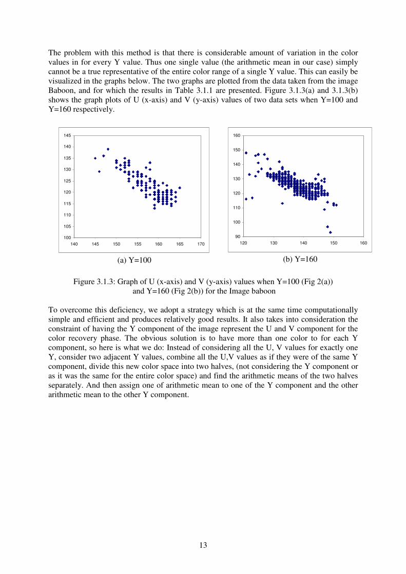
The problem with this method is that there is considerable amount of variation in the color values in for every Y value. Thus one single value (the arithmetic mean in our case) simply cannot be a true representative of the entire color range of a single Y value. This can easily be visualized in the graphs below. The two graphs are plotted from the data taken from the image Baboon, and for which the results in Table 3.1.1 are presented. Figure 3.1.3(a) and 3.1.3(b) shows the graph plots of U (x-axis) and V (y-axis) values of two data sets when Y=100 and Y=160 respectively.

Figure 3.1.3: Graph of U (x-axis) and V (y-axis) values when Y=100 (Fig 2(a))

and Y=160 (Fig 2(b)) for the Image baboon To overcome this deficiency, we adopt a strategy which is at the same time computationally simple and efficient and produces relatively good results. It also takes into consideration the constraint of having the Y component of the image represent the U and V component for the color recovery phase. The obvious solution is to have more than one color to for each Y component, so here is what we do: Instead of considering all the U, V values for exactly one Y, consider two adjacent Y values, combine all the U,V values as if they were of the same Y component, divide this new color space into two halves, (not considering the Y component or as it was the same for the entire color space) and find the arithmetic means of the two halves separately. And then assign one of arithmetic mean to one of the Y component and the other arithmetic mean to the other Y component.

100

105

110

115

120

125

130

135

140

145

140 145 150 155 160 165 170

(a) Y=100

90

100

110

120

130

140

150

160

120 130 140 150 160

(b) Y=160

14

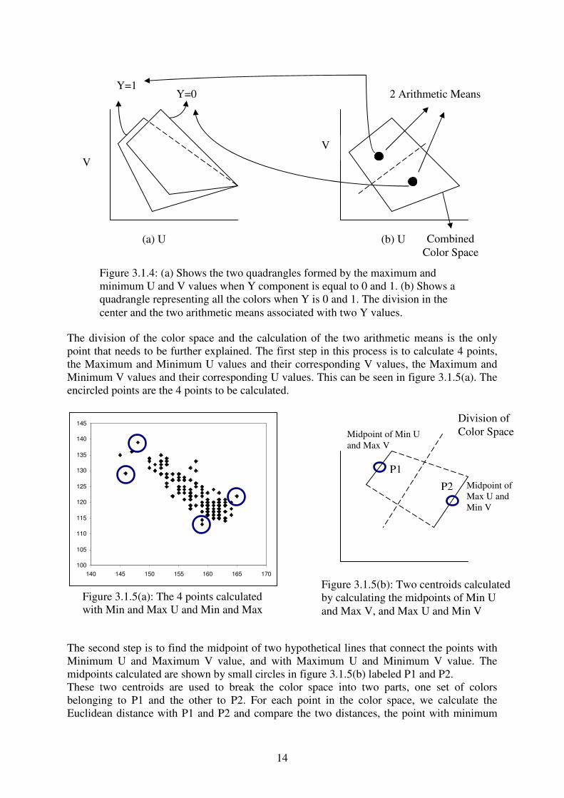
The division of the color space and the calculation of the two arithmetic means is the only point that needs to be further explained. The first step in this process is to calculate 4 points, the Maximum and Minimum U values and their corresponding V values, the Maximum and Minimum V values and their corresponding U values. This can be seen in figure 3.1.5(a). The encircled points are the 4 points to be calculated.

100

105

110

115

120

125

130

135

140

145

140 145 150 155 160 165 170

The second step is to find the midpoint of two hypothetical lines that connect the points with Minimum U and Maximum V value, and with Maximum U and Minimum V value. The midpoints calculated are shown by small circles in figure 3.1.5(b) labeled P1 and P2. These two centroids are used to break the color space into two parts, one set of colors belonging to P1 and the other to P2. For each point in the color space, we calculate the Euclidean distance with P1 and P2 and compare the two distances, the point with minimum

(a) U

V

Y=0 Y=1

V

(b) U

2 Arithmetic Means

Figure 3.1.4: (a) Shows the two quadrangles formed by the maximum and minimum U and V values when Y component is equal to 0 and 1. (b) Shows a quadrangle representing all the colors when Y is 0 and 1. The division in the center and the two arithmetic means associated with two Y values.

Combined Color Space

Figure 3.1.5(a): The 4 points calculated with Min and Max U and Min and Max V

Figure 3.1.5(b): Two centroids calculated by calculating the midpoints of Min U and Max V, and Max U and Min V

Midpoint of Min U and Max V

Midpoint of Max U and Min V

P1 P2

Division of Color Space

15

distance suggesting that it belongs to that division. After separating colors in this manner, we simply calculate the arithmetic mean of all the points in each division separately. And simply associate one arithmetic mean to one of the Y component and the other arithmetic mean to the other Y component, and in this manner creating a color palette. Table 3.1.3 shows the results when this technique is used to create a color palette.

Serial No.


PSNR SSIM 1 Airplane 32.69 dB 95.85% 2 Baboon 22.52 dB 82.82% 3 Day 29.69 dB 95.81% 4 Football 26.00 dB 89.26% 5 House 30.57 dB 89.49% 6 Lena 30.85 dB 93.55% 7 Peppers 28.20 dB 89.90%

Table 3.1.3: Objective Measures; Original Color image and the Reconstructed Color image using two layers at a time

But since this strategy doesn’t keep the original luminance values of the color image and changes the values according to the color palette constructed, we need to do a bit of processing to actually find the Index Image. We start with the image in YUV color space. The next step is to take every pixel in the Color image, find the closest color to it in the color palette and use the Y component in the color palette in place of the actual luminance value and thus in this manner we eventually obtain a luminance image which is close to the original luminance image. This new image serves as the Index Image. This changing of luminance values from the actual values keeps the bijection between the Y component and the Color palette as every Y value in the Index image points to a Color in the Palette which is close to the original color in the color image. The table below (Table 3.1.4) shows the PSNR of the paintings converted to gray scale image from RGB color space and their corresponding Luminance image in Column 1 and Index image in Column 2. It is quite clear from the high PSNR values in Table 3.1.4 that changing the luminosity (Y) component to obtain the index image doesn’t degrade the quality of the luminance image to a large extent.

PSNR Serial No.

Image Name

Gray level image and Luminance Image

Column 1

Luminance image and Index Image

Column 2

Gray Level image and Index Image

Column 3 1 Airplane 51.06 dB 46.48 dB 46.48 dB 2 Baboon 51.48 dB 43.22 dB 43.46 dB 3 Day 51.50 dB 45.38 dB 45.58 dB 4 Football 50.74 dB 44.44 dB 43.94 dB 5 House 51.25 dB 45.33 dB 45.30 dB 6 Lena 53.08 dB 44.14 dB 44.32 dB 7 Peppers 52.37 dB 44.01 dB 44.15 dB

Table 3.1.4: PSNR between Gray image, Luminance and Index image using two layers at a time.

16

The table below (Table 3.1.5) shows the SSIM of the paintings converted to gray scale image from RGB color space and their corresponding Luminance image in Column 1 and Index image in Column 2. Again from the high percentages in Table 3.1.5 show that changing the luminosity (Y) component to obtain the index image doesn’t degrade the quality of the luminance image to a large extent.

SSIM Serial No.

Image Name

Gray level image and Luminance Image

Column 1

Luminance image and Index Image

Column 2

Gray Level image and Index Image

Column 3 1 Airplane 99.81% 99.38% 99.25% 2 Baboon 99.95% 99.51% 99.46% 3 Day 99.93% 99.60% 99.55% 4 Football 99.88% 99.34% 99.27% 5 House 99.79% 98.94% 98.75% 6 Lena 99.87% 98.97% 98.86% 7 Peppers 99.86% 99.05% 98.95%

Table 3.1.5: SSIM between Gray image, Luminance and Index image The tables 3.1.1 to 3.1.5 can be used to deduce a simple relation, as we increase the number of layers, we will have more colors in the color palette and thus the objective measures will show better results in terms of comparing the original color images with the reconstructed color images. But on the contrary, since we will end up changing the luminance values the, objective measures will show a decrease in the similarity of the grey level image and the index image. We intend to study this relation and find out the behavior as we increase the number of clusters/layers used to generate the color palette as a function of the objective measures, the PSNR and the SSIM. Further experimentation was done with the above described technique using three, four and five layers at a time; for the set of images used for experimentation. We plot a graph with the number of layers used to generate the color palette as the independent variable and the sum of PSNR values (Original Color Image and the Reconstructed Color Image) as the dependent variable shown in Figure 3.1.6 (a). from the graph below, it is clear that the best results can be obtained when three layers are taken at a time to generate three different colors.

160

170

180

190

200

210

220

230

1 2 3 4 5

Figure 3.1.6 (a): For Original Color Image and reconstructed Image

Number of Levels and Sum of PSNR of all images

17

200

220

240

260

280

300

320

340

360

380

1 2 3 4 5

Figure 3.1.6 (b): For Gray Level Image and Index Image Number of Levels and Sum of PSNR of all images

Figure 3.1.6 (b) shows the graph of the Number of Levels taken at a time and the sum of PSNR values between the grey level image and the index image. The values are almost equal when two or three layers are considered (results being slightly better when three layers are considered). Thus from figure 3.1.6 (a) and (b) we can conclude that the results are better in the case where we consider three layers at a time and generate three different colors. An explanation of this method is followed; Here is what we did; we take three consecutive Y values each time, combine them to form a single color space (Figure 3.1.7 (a)), then find the four corners of this new combined color space by finding the maximum U, V values (and corresponding V value) and minimum U, V values (corresponding U values), we call them P1, P2, P3 and P4 (Figure 3.1.7 (b)).

(a) U

V

Y=0

V

(b) U


Y=2 4 Corners of the Combined Color Space

P1

P2

P4

P3

Y=1

Figure 3.1.7: (a) Shows the three quadrangles showing the color space formed when Y is equal to 0, 1 and 2 (b) Shows a quadrangle representing all the colors when Y is between 0 and 2 inclusive. The fours corners are found of the color space

18

The next step is to calculate the mid points of the hypothetical lines between the points P1 and P2, and the midpoint of P3 and P4. Also calculate the midpoint of these two midpoints thus giving us a point in the middle. These three points are shown in Figure 3.1.7 (c). Then we divide this new color space with respect to these three points, that is for every point in the color space, we calculate the distance with these three points and associate it to one of these three points. Once we have done that, we calculate the arithmetic mean of the color spaces to find a U,V value for each division (Figure 3.1.7 (d)). Finally we associate each arithmetic mean to a Y, thus the color palette is constructed in this way. Listing 3.1.1 shows the algorithm.

V

U

(c) (d) Figure 3.1.7 (c) Shows the three midpoints (b) shows the arithmetic mean associated to a Y.

U

Y=0 Y=1

Y=2

3 Different Colors

V

Algorithm Construct Palette: Color Image in YUV color space as parameter

1. Initialize a variable J with 0 2. Separate All the colors having Y component equal to J, J+1, J+2 call this array Color 3. Find 4 points, having the maximum and minimum U value (and corresponding V

values) and having the maximum and minimum V value (and corresponding U values) in array Color. Call these points P1, P2, P3, P4.

4. Calculate the midpoint of P1 and P2, and the midpoint of P3 and P4 and the midpoint of these two midpoints, call them M1, M2, M3.

5. Calculate for all points in array Color whether they are close to M1, M2, P3 using the Euclidean distance formula.

6. Calculate the Arithmetic mean of all the points close to M1, M2 and M3 separately. Call these arithmetic means A1, A2 and A3. Associate A1 to J (as Y component) A2 to J+1 (as Y component), A3 to J+2.

7. Repeat from step 2 with J=J+3 until J=255

Listing 3.1.1: The algorithm to construct the color palette.


19

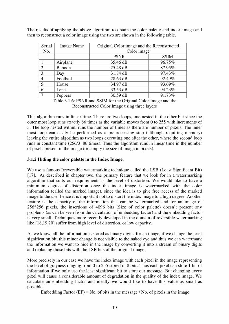
The results of applying the above algorithm to obtain the color palette and index image and then to reconstruct a color image using the two are shown in the following table.

Serial No.


PSNR SSIM 1 Airplane 35.46 dB 96.75% 2 Baboon 25.48 dB 87.95% 3 Day 31.84 dB 97.43% 4 Football 28.63 dB 92.49% 5 House 34.97 dB 93.69% 6 Lena 33.53 dB 94.23% 7 Peppers 30.59 dB 91.73%

Table 3.1.6: PSNR and SSIM for the Original Color Image and the Reconstructed Color Image using three layers

This algorithm runs in linear time. There are two loops, one nested in the other but since the outer most loop runs exactly 86 times as the variable moves from 0 to 255 with increments of 3. The loop nested within, runs the number of times as there are number of pixels. The inner most loop can easily be performed as a preprocessing step (although requiring memory) leaving the entire algorithm as two loops executing one after the other, where the second loop runs in constant time (256/3=86 times). Thus the algorithm runs in linear time in the number of pixels present in the image (or simply the size of image in pixels). 3.1.2 Hiding the color palette in the Index Image. We use a famous Irreversible watermarking technique called the LSB (Least Significant Bit) [17]. As described in chapter two, the primary feature that we look for in a watermarking algorithm that suits our requirements is the level of distortion. We would like to have a minimum degree of distortion once the index image is watermarked with the color information (called the marked image), since the idea is to give free access of the marked image to the user hence it is important not to distort the index image to a high degree. Another feature is the capacity of the information that can be watermarked and for an image of 256*256 pixels, the insertions of 4096 bits (Size of color palette) doesn’t present any problems (as can be seen from the calculation of embedding factor) and the embedding factor is very small. Techniques more recently developed in the domain of reversible watermarking like [18,19,20] suffer from high level of distortion, or low capacity. As we know, all the information is stored as binary digits, for an image, if we change the least signification bit, this minor change is not visible to the naked eye and thus we can watermark the information we want to hide in the image by converting it into a stream of binary digits and replacing those bits with the LSB bits of the original image. More precisely in our case we have the index image with each pixel in the image representing the level of grayness ranging from 0 to 255 stored in 8 bits. Thus each pixel can store 1 bit of information if we only use the least significant bit to store our message. But changing every pixel will cause a considerable amount of degradation in the quality of the index image. We calculate an embedding factor and ideally we would like to have this value as small as possible.

Embedding Factor (EF) = No. of bits in the message / No. of pixels in the image

20

Since our color palette consists of only U and V values, each 8 bits long, the total size of our color palette would be:

Size of Color Palette in Bits= 2 * 8 * 256 = 4096 bits The Number of pixels in an image depend on the dimensions of the image that we are working on, in our case, all the images that we are working on are of the dimension 256 * 256, so we have an image of 65536 pixels.

EF = 4096 / 65536 = 1 / 16 = 0.0625 bit / pixel From the EF, we can calculate the size of the number of pixels that we need to store one bit of the message, we call this a block of pixels to store One bit of data. Size of Block = 1 / 0.0625 = 16 pixel / bit Once we know the size of a block, we take a number input from the user, which will serve as the key or the secret code to retrieve the hidden color palette from the image in the color recovery phase. From that number, we generate a series of random numbers between 0 and 4096. We track collisions and generate only a number once, this series gives us the block numbers to store our message. For every block we take the first pixel and replace the least significant bit with our message. In the case where the message bit is equal to the data bit, there is simply no change but in the case where the information to be embedded is different from the data bit, we effectively break the bijection between the index image and the color palette, as the Y value no longer points out to the color in the color palette that it should. In order to ensure the bijection, we do a bit of processing in the color palette. Since we know that after a difference of two colors in the color palette, the colors are very close to each other, we simply swap colors to put two colors that are close, adjacent to each other and thus we adjust the index image appropriately. Thus before we can embed the information in the index image, we change the color palette, adjust the index image and then use the LSB algorithm to embed the information.

Algorithm Watermarking: Input Index Image and Color Palette as bit stream

1. Calculate the Number of bits in the Message 2. Calculate the Number of Pixels in the Image 3. Calculate the Embedding factor and Size of Block 4. If size of block is less than 1, display message “image too small to embed the

message” and exit from function. 5. Input a number from the user and generate a series of random numbers between 0

and Size of Message with no repeated number. This series gives us the blocks to embed data.

6. Take a number from the series to give the block to start embedding data. 7. Take the first pixel in the block and see if the LSB is equal to the data bit to be

embedded, if they are not equal go to step 8 otherwise go to step 9. 8. See which color needs to be coded for the pixel and appropriately add 1 or subtract

1 from the Pixel Value. 9. Until series is not finished, take the next number from the series and repeat step 6.

Listing 3.1.2: Algorithm for hiding the color palette in the Index Image to generate Marked Image

21

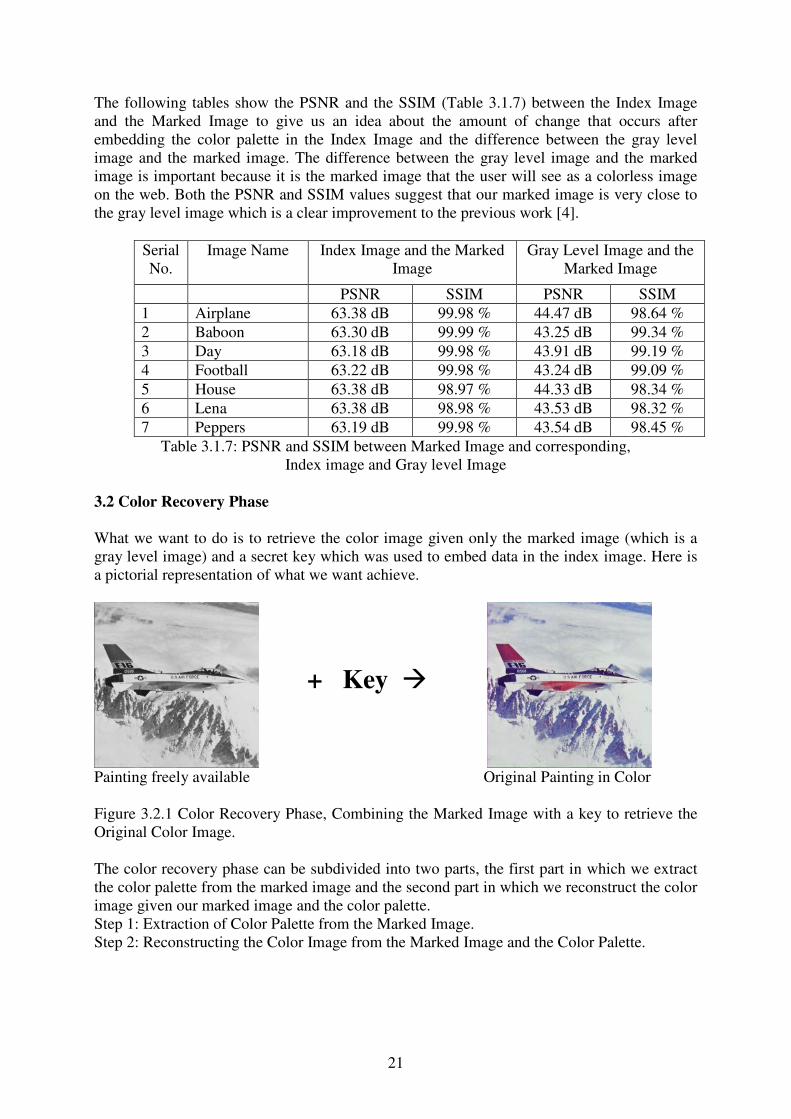
The following tables show the PSNR and the SSIM (Table 3.1.7) between the Index Image and the Marked Image to give us an idea about the amount of change that occurs after embedding the color palette in the Index Image and the difference between the gray level image and the marked image. The difference between the gray level image and the marked image is important because it is the marked image that the user will see as a colorless image on the web. Both the PSNR and SSIM values suggest that our marked image is very close to the gray level image which is a clear improvement to the previous work [4].

Serial No.

Image Name Index Image and the Marked Image

Gray Level Image and the Marked Image

PSNR SSIM PSNR SSIM 1 Airplane 63.38 dB 99.98 % 44.47 dB 98.64 % 2 Baboon 63.30 dB 99.99 % 43.25 dB 99.34 % 3 Day 63.18 dB 99.98 % 43.91 dB 99.19 % 4 Football 63.22 dB 99.98 % 43.24 dB 99.09 % 5 House 63.38 dB 98.97 % 44.33 dB 98.34 % 6 Lena 63.38 dB 98.98 % 43.53 dB 98.32 % 7 Peppers 63.19 dB 99.98 % 43.54 dB 98.45 %

Table 3.1.7: PSNR and SSIM between Marked Image and corresponding, Index image and Gray level Image

3.2 Color Recovery Phase What we want to do is to retrieve the color image given only the marked image (which is a gray level image) and a secret key which was used to embed data in the index image. Here is a pictorial representation of what we want achieve.

Painting freely available Original Painting in Color Figure 3.2.1 Color Recovery Phase, Combining the Marked Image with a key to retrieve the Original Color Image. The color recovery phase can be subdivided into two parts, the first part in which we extract the color palette from the marked image and the second part in which we reconstruct the color image given our marked image and the color palette. Step 1: Extraction of Color Palette from the Marked Image. Step 2: Reconstructing the Color Image from the Marked Image and the Color Palette.

+ Key �

22

Figure 3.2.2: Extracting Color palette from the Marked Image and reconstructing the Original

Color Image. 3.2.1 Extraction of Color Palette from the Marked Image. The idea is first to extract the hidden color palette from the Marked Image. In order to do so, the user feeds in the key and a series of random numbers is generated between 0 and size of message that was embedded in the image with no number repeated more than once. This series gives us the block numbers in which date was hidden and the corresponding sequence of the data. Reading the last bit of the first pixel in each block gives us the bit sequence of the message, which in our case is the color palette. 3.2.2 Reconstructing the Color Image from the Marked Image and the Color Palette. To reconstruct the color image from the Marked image, and the color palette, all we need to do is for every pixel value in the marked image, ranging from 0-255, look up in the color palette the values of U and V component and using the YUV values, reconstruct the color image in RGB color space. Table 3.2.1 represents the results when the color image is reconstructed in this manner. We calculate the PSNR and the SSIM value between the original color image and the reconstructed color image (from the marked image). Figure 3.2.3 shows the original color image, the reconstructed color image, the gray level image and the watermarked image for the two sample images Airplane and Baboon along with the corresponding objective measures.

Serial No.

Image Name Original Color Image and Reconstructed Color Image

PSNR SSIM 1 Airplane 34.99 dB 95.99 % 2 Baboon 25.45 dB 87.71 % 3 Day 31.67 dB 96.99 % 4 Football 28.45 dB 91.98 % 5 House 31.49 dB 91.60 % 6 Lena 33.39 dB 93.71 % 7 Peppers 30.27 dB 90.19 %

Table 3.2.1: PSNR between Original Color Image and Reconstructed Color Image

23

Following images showing the Original Color images, Reconstructed Color Images, the Luminance Image and the Indexed Image of two samples, Baboon and Airplane.

(a) Original Color Image (b) Reconstructed Color Image

(c) Gray Level Image (d) Marked Image

(e) Original Color Image (f) Reconstructed Color Image

(g) Gray Level Image (h) Marked Image Figure 3.2.3: Images showing the results of the first stage of the project, the Color hiding and

Recovery Phase for the two sample images with the best and worst PSNR values.

PSNR = 25.45 dB SSIM = 87.71 %

PSNR = 43.25 dB SSIM = 99.34 %

PSNR = 34.99 dB SSIM = 95.99 %

PSNR = 44.47 dB SSIM = 98.64 %

24

3.3 Findings and Comments As this chapter was divided into two sections the Color hiding phase and the Color recovery phase, we examine the work done in these two sections separately; In the first phase, the major steps were to quantify the color information and find a color palette, find an index image, and then hide the quantified color information in the index image to obtain the marked image. In terms of quantification of the color information, we found a new algorithm based on the luminance of the color image. This was specifically done so to obtain a gray level image which is close to the Luminance image and thus creating a bijection between the index image and the color palette. Then using the LSB algorithm, the color information was watermarked on the index image. The second phase is concerned with the extraction of the color palette and the reconstructing the color image from the marked image and the secret key. The results in figure 3.2.3 show that the Marked image is very close to the gray level image both in terms of the SSIM and the PSNR. Thus one of the primary objectives of this research was attained to have a method which produces a good quality gray level image (in this case the marked image). High SSIM values for the color image and the reconstructed image show that the results obtained by the application of this method produce good results but in terms of PSNR value, especially for the image Baboon, even visually, it is quite visible that there is a considerable loss in the color information due to the process of color quantization.

25

Chapter Four: Study robustness of the Marked Image with respect to Image Compression

The second stage is to study the robustness of the Marked Image with respect to JPEG and JPEG-2000 image compression. The idea is to be able to compress the Marked Image, obtained as a result of Color Hiding Phase (see figure 3.1.1), decompress it and still be able to reconstruct the color image. That is in between the Color Hiding Phase and the Color Recovery Phase; we want to embed the phase of Compression and Decompression and study how our method holds up to the distortion created by compression of the marked image. In the first section we study the effect of the image compression on the marked image and the resulting reconstructed color image and in the following sections we present two different methods to increase the robustness of the proposed method with respect to image compression. Here is the pictorial representation of what we want to achieve.

Figure 4.1: Showing the basic idea of what we want to study in the second stage of the Project 4.1 Compressing Marked Image using Jpeg and Jpeg -2000 As described briefly, the idea is to be able to embed the compression and decompression phase in between the color hiding phase and the color recovery phase. To do, we take the Original color image, find a color palette using the method described in chapter 1, and hide it in the index image to obtain the marked image. Once we have the marked image, we compress it using the compression schemes (Jpeg and Jpeg 2000) with different values of Quality Measure. Quality measure is a parameter which ranges between 0 and 100% and depicts the values from High compression – Low quality image to Low Compression – High quality image. For example, the value 100% suggests that the level of compression of the given image was the lowest (but still there was a lossless compression) but the quality of the image was the highest (although there was some loss as compared to the uncompressed image).

Decompress Compress

Reconstructed Color Image from Marked Image (after Compression)

Marked Image Marked Image

26

Figure 4.1.1: Showing the steps to be performed in the second stage of the Project Table 4.1.1 present the results for the sample image Airplane if JPEG compression is used for different values of Quality Measure. From the PSNR and SSIM values, it is quite obvious that the loss of data because of JPEG compression changes the color palette and thus the resulting reconstructed image is degraded badly as compared to the reconstructed image without JPEG compression. Compression Scheme JPEG Image: Airplane Dimensions: 256 * 256 pixels Quality Measure

Size of Marked Image

Original Color Image and Reconstructed Color Image

after Compression

Reconstructed Color Image without compression and Reconstructed Color Image after Compression

PSNR SSIM PSNR SSIM Without Compres.

34.99 dB

95.99 %

�

100 %

100% 42.1 Kb 16.62 dB 33.39 % 13.11 dB 22.52 % 95% 25.1 Kb 10.06 dB 10.20 % 9.61 dB 8.81 % 90% 18.0 Kb 11.01 dB 11.64 % 10.01 dB 9.91 % 80% 12.5 Kb 9.93 dB 10.18 % 11.05 dB 12.39 % 50% 7.50 Kb 9.10 dB 12.74 % 11.23 dB 16.81 % Table 4.1.1: PSNR and SSIM of the reconstructed image after different levels of compression

with the Original Color image and the Reconstructed Color image without Compression In case of JPEG-2000, the results (Table 4.1.2) in general are not much different as compared to JPEG compression, although marginally better, but still the image reconstructed is very much distorted. The only positive aspect of trying the JPEG-2000 is that since there is an option of lossless compression in JPEG-2000 which obviously restores the image in color as it was never compressed but still it reduces the file size to 36.9 kb from 64 Kb which is a reduction of 33.3 % in the file size. We can conclude that using the JPEG-2000 format with a

Compress

Decompress

Original Color Img

Index Img

Marked Img

Marked Img

Reconstructed Color Img after Compression

Reconstructed Color Img without compression

Color Palette

27

lossless compression reduces the size as well as maintains the integrity of the color palette hidden within the image. Compression Scheme JPEG – 2000 Image: Airplane Dimensions: 256 * 256 pixels Quality Measure

Size of Marked Image

Original Color Image and Reconstructed Color Image

after Compression

Reconstructed Color Image without compression and Reconstructed Color Image after Compression

PSNR SSIM PSNR SSIM Without Compres

64.0 Kb

34.99 dB

95.99 %

�

100 %

Lossless Compres.

36.9 Kb

34.99 dB

95.99 %

�

100 %

100% 29.0 Kb 10.61 dB 10.40 % 10.64 dB 10.45 % 95% 25.4 Kb 9.77 dB 9.79 % 9.79 dB 9.84 % 90% 22.4 Kb 9.59 dB 8.97 % 9.62 dB 9.00 % 80% 17.5 Kb 10.43 dB 10.50 % 10.46 dB 10.44 % 50% 9.19 Kb 10.18 dB 13.21 % 10.20 dB 13.17 % Table 4.1.2: PSNR and SSIM of the reconstructed image after different levels of compression

with the Original Color image and the Reconstructed Color image without Compression 4.2 Using DWT to increase robustness with respect to Image Compression To increase the robustness of our method with respect to image compression, what we try to do is to perform a decomposition of level ‘n’. We know that the DWT split a component into numerous frequency bands called sub bands and for each level DWT is applied twice, once row-wise and once column-wise resulting in four sub bands namely 1) horizontally and vertically lowpass (LL), 2) horizontally lowpass and vertically highpass (LH), 3) horizontally highpass and vertically lowpass (HL), and 4) horizontally and vertically highpass (HH). What we do is reduce the original color image by a factor ‘n’, perform a DWT of level ‘n’. From the reduced size color image, obtain a marked image (from the method described in Chapter 1) which is a marked image of reduced size. Then we replace the LL subband with this marked image and perform an inverse DWT transform to obtain the final marked image which we will use as grey level image freely accessible to the users. Figure 4.2.1 shows the steps performed in the procedure described above.

28

Figure 4.2.1: Steps to increase robustness with respect to image compression using DWT Table 4.2.1 shows the results of applying the above technique with level 1 decomposition. Since we want to keep a constant embedding factor (see chapter 1) of 1/16, and we know that the size of our color palette remains constant (4096 bits), thus we start the process with an image of 512 * 512 pixels.

Compress

Decompress

Reduced Size Color Img

Index Img

Marked Img

Marked Img

Reconstructed Color Img after Compression

Y DWT level 1

DWT-1 level 1

Marked Img

DWT level 1

Original Size Reconstructed

Color Img after Compression

Increase Size

Original Color Img

29

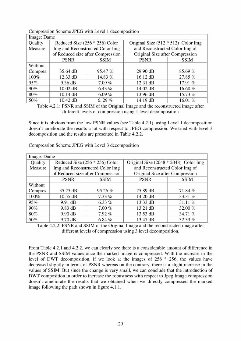
Compression Scheme JPEG with Level 1 decomposition Image: Dame Quality Measure

Reduced Size (256 * 256) Color Img and Reconstructed Color Img of Reduced size after Compression

Original Size (512 * 512) Color Img and Reconstructed Color Img of Original Size after Compression


35.64 dB

95.47 %

29.90 dB

85.69 %

100% 12.33 dB 14.83 % 16.12 dB 27.85 % 95% 9.36 dB 7.09 % 12.31 dB 17.91 % 90% 10.02 dB 6.43 % 14.02 dB 16.68 % 80% 10.14 dB 6.09 % 13.96 dB 15.73 % 50% 10.42 dB 6. 29 % 14.19 dB 16.01 %

Table 4.2.1: PSNR and SSIM of the Original Image and the reconstructed image after different levels of compression using 1 level decomposition

Since it is obvious from the low PSNR values (see Table 4.2.1), using Level 1 decomposition doesn’t ameliorate the results a lot with respect to JPEG compression. We tried with level 3 decomposition and the results are presented in Table 4.2.2. Compression Scheme JPEG with Level 3 decomposition Image: Dame Quality Measure

Reduced Size (256 * 256) Color Img and Reconstructed Color Img of Reduced size after Compression

Original Size (2048 * 2048) Color Img and Reconstructed Color Img of Original Size after Compression


35.25 dB

95.26 %

25.89 dB

71.84 %

100% 10.55 dB 7.33 % 14.20 dB 33.31 % 95% 9.91 dB 6.33 % 13.33 dB 31.11 % 90% 9.83 dB 7.00 % 13.21 dB 32.00 % 80% 9.90 dB 7.92 % 13.53 dB 34.71 % 50% 9.70 dB 6.84 % 13.47 dB 32.33 %

Table 4.2.2: PSNR and SSIM of the Original Image and the reconstructed image after different levels of compression using 3 level decomposition.

From Table 4.2.1 and 4.2.2, we can clearly see there is a considerable amount of difference in the PSNR and SSIM values once the marked image is compressed. With the increase in the level of DWT decomposition, if we look at the images of 256 * 256, the values have decreased slightly in terms of PSNR whereas on the contrary, there is a slight increase in the values of SSIM. But since the change is very small, we can conclude that the introduction of DWT composition in order to increase the robustness with respect to Jpeg Image compression doesn’t ameliorate the results that we obtained when we directly compressed the marked image following the path shown in figure 4.1.1.

30

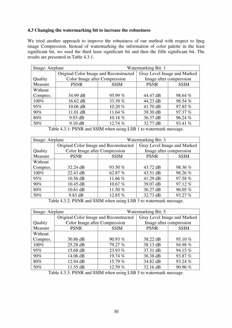
4.3 Changing the watermarking bit to increase the robustness We tried another approach to improve the robustness of our method with respect to Jpeg image Compression. Instead of watermarking the information of color palette in the least significant bit, we used the third least significant bit and then the fifth significant bit. The results are presented in Table 4.3.1.

Image: Airplane Watermarking Bit: 1 Original Color Image and Reconstructed

Color Image after Compression Gray Level Image and Marked

Image after compression Quality Measure PSNR SSIM PSNR SSIM Without Compres.

34.99 dB

95.99 %

44.47 dB

98.64 %


Table 4.3.1: PSNR and SSIM when using LSB 1 to watermark message.




32.24 dB

93.50 %

43.72 dB

98.36 %






30.86 dB

90.93 %

38.22 dB

95.10 %



31

We tried to embed the information in the seventh and the eighth bit as well but the distortion caused due to this insertion was visually quite disturbing, in fact, even with the insertion in the fifth bit, we clearly see the distortion created in the marked image as well as the reconstructed image (Figure 4.3.1). Although there was a slight improvement in the robustness of the marked image with respect to Jpeg compression but still the low PSNR values for the reconstructed color image suggest that changing the bit to watermark the color information doesn’t really increase the robustness of the proposed method with respect to jpeg image compression. If we look at the PSNR and SSIM values for the gray level image and the marked image, they are very high suggesting that even if the fifth bit is used to watermark the information, the degradation in the quality of the marked image is very little, thus we can conclude that it’s actually the color palette that is lost by the image compression and obviously the bijection of the marked image and the color palette doesn’t resist the image compression. The figures below show the images obtained after the changing the watermarking bit and using different Quality Measure (QM).

(a) Original Color Image (b) Without Compression PSNR= 34.99 dB SSIM= 95.99 %

(c) QM=100% (d) QM=50% PSNR= 16.62 dB SSIM= 33.39 % PSNR= 9.10 dB SSIM= 12.74 %

Figure 4.3.1: Original Color Image and the Reconstructed Color Images when Watermarking bit is 1, with different QM

32

(a) Original Color Image (b) Without Compression PSNR= 30.86 dB SSIM= 90.93 %

(c) QM=100% (d) QM=50% PSNR= 25.28 dB SSIM= 79.27 % PSNR= 11.55 dB SSIM= 12.59 %

Figure 4.3.2: Original Color Image and the Reconstructed Color Images when Watermarking bit is 5, with different QM

Comparing Figure 4.3.1 and 4.3.2, with respect to objective measures as well as visually we see a little improvement in the level of distortion caused due to jpeg image compression but still the level of distortion is considerably high, especially when the quality measure falls below 100% as can be seen in tables 4.3.1 to 4.3.3. 4.4 Findings and Comments We study the effect of compressing the marked image with respect to jpeg and jpeg 2000 image compression schemes. As can be seen from the low PSNR and SSIM values in table 4.1.1 and 4.1.2, the proposed method doesn’t resist any sort of lossless image compression, although if the quality measure is set to 100%, there is some sort of resistance but as the quality measure is decreased, the quality of the reconstructed color image decreases also. We proposed two different methods to ameliorate the resistance with respect to image compression. The first method is using the Discrete wavelet transform, where we try to decompose the image and replace the LL sub-band with the marked image, table 4.2.1 and 4.2.2 present the results using different levels of decomposition and there is no considerable improvement to the method. The second method tried to improve the robustness was changing the LSB bit, and using different bits to embed the watermarking information. The results using different bits are presented in table 4.3.1 to 4.3.3 and the low PSNR and SSIM suggest there is an improvement if the quality measure remains 100%, but as soon as the quality measure is decreased from 100%, the quality of the reconstructed image drops significantly and thus producing poor overall results.

33

References: [1] M. Chaumont and W. Puech, “A Color Image in a Gray-Level Image”, in IS&T Third European Conference on Colour in Graphics, Imaging and Vision, CGIV’2006, Leeds, UK, June 2006, pp. 226-331 [2] R. de Queiroz and K Braun, “Color to Gray and Back: Color Embedding Into Textured Gray Images”, IEEE Transaction on Image Processing, vol. 15, no. 6, pp. 1464-1470, 2006. [3] P. Campisi, D. Kundur, D. Hatzinakos and A. Neri, “Compressive Data Hiding: An Unconventional Approach for improved Color Image Coding”, EURASIP journal on Applied Signal Processing, vol. 2002, no. 2, pp. 152-163,2002. [4] M. Chaumont and W. Puech, “A fast and efficient method to protect color images”, VCIP’2007 SPIE’2007, Visual Communication and Image Processing, Part of the IS&T/SPIE on Electronic Imaging, San Jose, California, USA, 28 January – 1 February 2007. [5] M. Chaumont and W. Puech, “A DCT-Based Data-Hiding Method to Embed the Color Information in a JPEG Grey Level Image”, EUSIPCO’2006, The European Signal Processing Conference, Pise, Italy September 2006. [6] M. Chaumont et W. Puech, “Une image couleur cachée dans une image en niveaux de gris”, COmpression et REprésentation des Signaux Audiovisuels, CORESA’2006, Novembre 2006. [7] D. Coltuc, J-M. Chassery, “Distortion Control Reversible Watermarking”, Second International Symposium on Communications, Control and Signal Processing, ISCCSP’O6, Marrakech, Morocco, 13-15 March 2006. [8] Gregory K. Wallace, “The JPEG still picture compression standard”, Special issue on digital multimedia systems Pages: 30 – 44, ACM Press, New York, NY, USA, 1991 [9] Michael D. Adams , “JPEG 2000 Still Image Compression Standard”, (Last Revised 2005-12-03). ISO/IEC JTC 1/SC 29/WG 1 (N 2412). [10] Jin Li, “Image Compression - The Mechanics of the JPEG 2000”, Microsoft Research, Signal Processing 2002. [11] Zhou Wang, Alan Conrad Bovik, Hamid Rahim Sheikh, Eero P. Simoncelli, “Image Quality Assessment: From Error Visibility to Structural Similarity”, IEEE Transactions on Image Processing, Vol. 13, NO. 4, APRIL 2004. [12] Gaurav Sharma, “Digital Color Imaging Handbook”, CRC Press LLC, 2003. [13] J. Fredrich, “A New Steganographic Method for Palette Based Images”, in Proceedings of the IS&T PICS conference, Apr,1998. [14] M.-Y. Wu, Y.-K. Ho and J.-H Lee, “An iterative Method of Palette-Based Image Steganography”, Pattern Recognition Letters, vol. 25, pp. 301-309, 2003.

34

[15] C.H. Tzeng, Z.F. Yang and W.H. Tsai, “Adaptive Data Hiding in Palette Images by Color Ordering and Mapping with Security Protection”, IEEE Transaction on Communications, vol. 52, no. 5, pp. 791-800, 2004. [16] E. Marini, F. Autrusseau, P.L. Callet, P. Campisi, “Evaluation of standard watermarking techniques”, in Proceedings of the SPIE, Vol 6505, pp. 65050O, 2007. [17] Edited by Stefan Katzenbeisser, Fabien A. P. Petitcolas, “Information Hiding Techniques for Steganography and Digital Watermarking”, ARTECH HOUSE, INC. 2000 [18] D. Coltuc, J-M. Chassery, “High Capacity Reversible Watermarking”, Proceedings of the IEEE International Conference on Image Processing ICIP’2006, Atlanta, GA, SUA, October 2006. [19] J. Fridrich, M. Goljan and R. Du, “Lossless Data Embedding – New Paradigm in Digital Watermarking”, Special Issue on Emerging Applications of Multimedia Data Hiding, Vol. 2002, No.2, February 2002, pp. 185–196. [20] J. Fridrich, M. Goljan, Q. Chen, and V. Pathak, “Lossless Data Embedding with File Size Preservation”, Proceedings EI SPIE San Jose, CA, Jan 2004.

35

Appendix A: Set of Images used for experimentation.

Airplane Baboon

Day Football

House Lena

Peppers Dame

Protection of Color Information of Images by Inserting...

Documents

Transcript of Protection of Color Information of Images by Inserting...