1. Propositional Logic

1.1. Basic Definitions.

Definition 1.1. The alphabet of propositional logic consists of

• Infinitely many propositional variables p0, p1, . . .,• The logical connectives ∧,∨,→,⊥, and• Parentheses ( and ).

We usually write p, q, r, . . . for propositional variables. ⊥ is pronounced“bottom”.

Definition 1.2. The formulas of propositional logic are given inductivelyby:

• Every propositional variable is a formula,• ⊥ is a formula,• If φ and ψ are formulas then so are (φ ∧ ψ), (φ ∨ ψ), (φ→ ψ).

We omit parentheses whenever they are not needed for clarity. We write¬φ as an abbreviation for φ → ⊥. We occasionally use φ ↔ ψ as anabbreviation for (φ→ ψ)∧ (ψ → φ). To limit the number of inductive caseswe need to write, we sometimes use ~ to mean “any of ∧,∨,→”.

The propositional variables together with ⊥ are collectively called atomicformulas.

1.2. Deductions. We want to study proofs of statements in propositionallogic. Naturally, in order to do this we will introduce a completely formaldefinition of a proof. To help distinguish between ordinary mathematicalproofs, written in (perhaps slightly stylized) natural language, and our for-mal notion, we will call the formal objects “deductions”.

Following standard usage, we will write ` φ to mean “there is a deductionof φ (in some particular formal system)”. We’ll often indicate the formalsystem in question either with a subscript or by writing it on the left of theturnstile: `c φ or Pc ` φ.

We will ultimately work exclusively in the system known as the sequentcalculus, which turns out to be very well suited to proof theory. However,to help motivate the system, we briefly discuss a few better known systems.

Probably the simplest family of formal systems to describe are Hilbertsystems. In a typical Hilbert system, a deduction is a list of formulas inwhich each formula is either an axiom from some fixed set of axioms, or anapplication of modus ponens to two previous elements on the list. A typicalaxiom might be

φ→ (ψ → (φ ∧ ψ)),

and so a deduction might consist of steps like...

(n) φ1

2

...(n’) φ→ (ψ → (φ ∧ ψ))

(n’+1) ψ → (φ ∧ ψ)...

(n”) ψ(n”+1) φ ∧ ψ

The linear structure of of Hilbert-style deductions, and the very simplelist of cases (each step can be only an axiom or an instance of modus ponens)makes it very easy to prove some theorems about Hilbert systems. Howeverthese systems are very far removed from ordinary mathematics, and theydon’t expose very much of the structure we will be interested in studying,and as a result are poorly suited to proof-theoretic work.

The second major family of formal systems are natural deduction systems.These were introduced by Gentzen in part to more closely resemble ordinarymathematical reasoning. These systems typically have relatively few axioms,and more rules, and also have a non-linear structure. One of the key featuresis that the rules tend to be organized into neat groups which help providesome meaning to the connectives. A common set-up is to have two rules foreach connective, an introduction rule and an elimination rule. For instance,the ∧ introduction rule states “given a deduction of φ and a deduction of ψ,deduce φ ∧ ψ”.

A standard way of writing such a rule is

φ ψ∧I

φ ∧ ψThe formulas above the line are the premises of the rule and the formula

below the line is the conclusion. The label simply states which rule is beingused. Note the non-linearity of this rule: we have two distinct deductions,one deduction of φ and one deduction of ψ, which are combined by this ruleinto a single deduction.

The corresponding elimination rules might be easy to guess:

φ ∧ ψ∧E1 φand

φ ∧ ψ∧E2 ψ

These rules have the pleasant feature of corresponding to how we actuallywork with conjunction: in an ordinary English proof of φ ∧ ψ, we wouldexpect to first prove φ, then prove ψ, and then note that their conjunctionfollows. And we would use φ∧ψ at some later stage of a proof by observingthat, since φ ∧ ψ is true, whichever of the conjuncts we need must also betrue.

This can help motivate rules for the other connectives. The eliminationrule for → is unsurprising:

3

φ φ→ ψ→ E

ψ

The introduction rule is harder. In English, a proof of an implicationwould read something like: “Assume φ. By various reasoning, we concludeψ. Therefore φ → ψ.” We need to incorporate the idea of reasoning underassumptions.

This leads us to the notion of a sequent. For the moment (we will modifythe definition slightly in the next section) a sequent consists of a set ofassumptions Γ, together with a conclusion φ, and is written

Γ⇒ φ.

Instead of deducing formulas, we’ll want to deduce sequents; ` Γ⇒ φ means“there is a deduction of φ from the assumptions Γ”. The rules of naturaldeduction should really be rules about sequents, so the four rules alreadymentioned should be:

Γ⇒ φ Γ⇒ ψ∧I

Γ⇒ φ ∧ ψΓ⇒ φ ∧ ψ∧E1 Γ⇒ φ

Γ⇒ φ ∧ ψ∧E2 Γ⇒ ψ

Γ⇒ φ Γ⇒ φ→ ψ→ E

Γ⇒ ψ

(Actually, in the rules with multiple premises, we’ll want to consider thepossibility that the two sub-derivations have different sets of assumptions,but we’ll ignore that complication for now.)

This gives us a natural choice for an introduction rule for →:

Γ ∪ {φ} ⇒ ψ→ I

Γ⇒ φ→ ψ

In plain English, “if we can deduce ψ from the assumptions Γ and φ, thenwe can also deduce φ→ ψ from just Γ”.

This notion of reasoning under assumptions also suggests what an axiommight be:

φ⇒ φ

(The line with nothing above it represents an axiom—from no premisesat all, we can conclude φ⇒ φ.) In English, “from the assumption φ, we canconclude φ”.

1.3. The Sequent Calculus. Our chosen system, however, is the sequentcalculus. The sequent calculus seems a bit strange at first, and gives upsome of the “naturalness” of natural deduction, but it will pay us back bybeing the system which makes the structural features of deductions mostexplicit. Since our main interest will be studying the formal properties ofdifferent deductions, this will be a worthwhile trade-off.

4

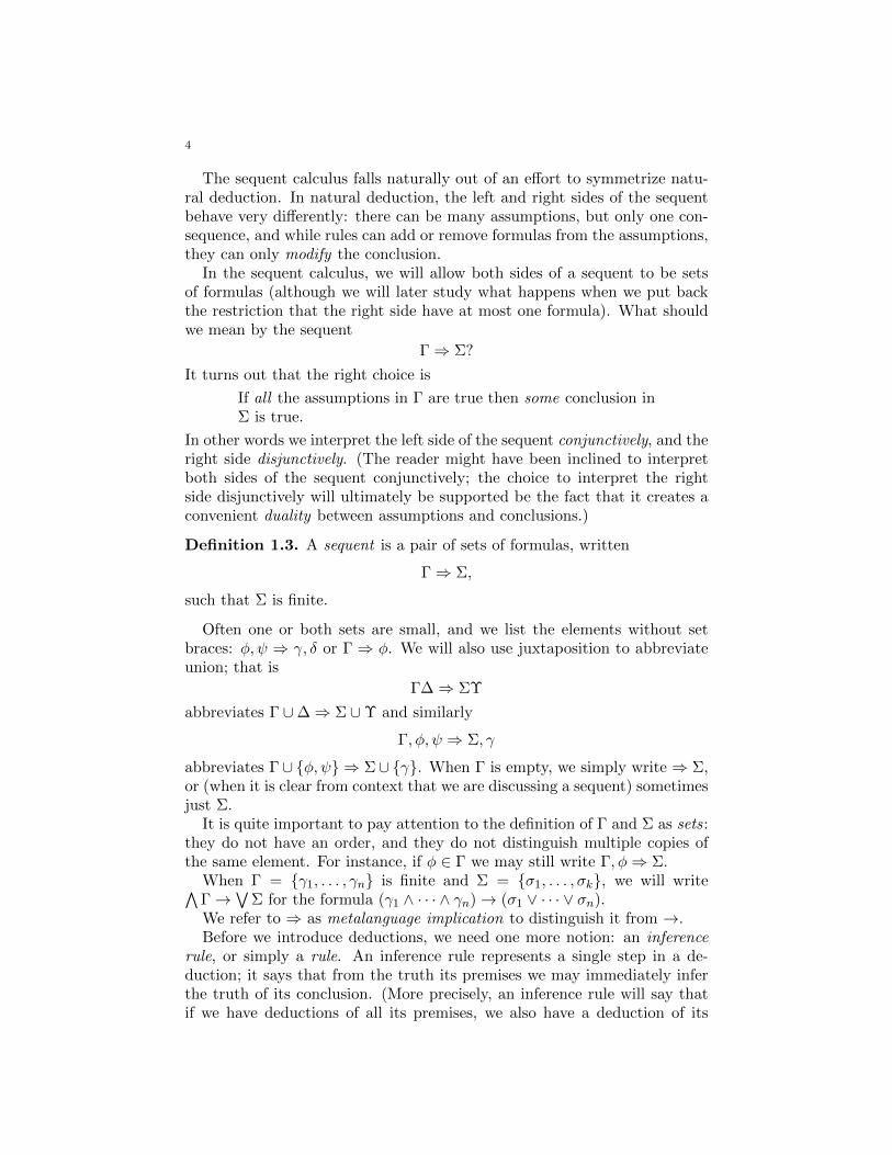
The sequent calculus falls naturally out of an effort to symmetrize natu-ral deduction. In natural deduction, the left and right sides of the sequentbehave very differently: there can be many assumptions, but only one con-sequence, and while rules can add or remove formulas from the assumptions,they can only modify the conclusion.

In the sequent calculus, we will allow both sides of a sequent to be setsof formulas (although we will later study what happens when we put backthe restriction that the right side have at most one formula). What shouldwe mean by the sequent

Γ⇒ Σ?

It turns out that the right choice is

If all the assumptions in Γ are true then some conclusion inΣ is true.

In other words we interpret the left side of the sequent conjunctively, and theright side disjunctively. (The reader might have been inclined to interpretboth sides of the sequent conjunctively; the choice to interpret the rightside disjunctively will ultimately be supported be the fact that it creates aconvenient duality between assumptions and conclusions.)

Definition 1.3. A sequent is a pair of sets of formulas, written

Γ⇒ Σ,

such that Σ is finite.

Often one or both sets are small, and we list the elements without setbraces: φ, ψ ⇒ γ, δ or Γ ⇒ φ. We will also use juxtaposition to abbreviateunion; that is

Γ∆⇒ ΣΥ

abbreviates Γ ∪∆⇒ Σ ∪Υ and similarly

Γ, φ, ψ ⇒ Σ, γ

abbreviates Γ∪ {φ, ψ} ⇒ Σ∪ {γ}. When Γ is empty, we simply write ⇒ Σ,or (when it is clear from context that we are discussing a sequent) sometimesjust Σ.

It is quite important to pay attention to the definition of Γ and Σ as sets:they do not have an order, and they do not distinguish multiple copies ofthe same element. For instance, if φ ∈ Γ we may still write Γ, φ⇒ Σ.

When Γ = {γ1, . . . , γn} is finite and Σ = {σ1, . . . , σk}, we will write∧Γ→

∨Σ for the formula (γ1 ∧ · · · ∧ γn)→ (σ1 ∨ · · · ∨ σn).

We refer to ⇒ as metalanguage implication to distinguish it from →.Before we introduce deductions, we need one more notion: an inference

rule, or simply a rule. An inference rule represents a single step in a de-duction; it says that from the truth its premises we may immediately inferthe truth of its conclusion. (More precisely, an inference rule will say thatif we have deductions of all its premises, we also have a deduction of its

5

conclusion.) For instance, we expect an inference rule which says that if weknow both φ and ψ then we also know φ ∧ ψ.

A rule is written like this:

Γ0 ⇒ ∆0 · · · Γn ⇒ ∆nName

Σ⇒ Υ

This rule indicates that if we have deductions of all the sequents Γi ⇒ ∆i

then we also have a deduction of Σ⇒ Υ.

Definition 1.4. Let R be a set of rules. We define R ` Σ⇒ Υ inductivelyby:

• If for every i ≤ n, R ` Γi ⇒ ∆i, and the rule above belongs to R,then R ` Σ⇒ Υ.

We will omit a particular set of rules R if it is clear from context.Our most important collection of inference rules for now will be classical

propositional logic, which we will call Pc. First we have a structural rule—arule with no real logical content, but only included to make sequents behaveproperly.

Γ⇒ ΣW

ΓΓ′ ⇒ ΣΣ′

W stands for “weakening”—the sequent ΓΓ′ ⇒ ΣΣ′ is weaker than thesequent Γ ⇒ Σ, so if we can deduce the latter, surely we can deduce theformer.

Pc will include two axioms (rules with no premises):

Axφ⇒ φ where φ is atomic.

L⊥ ⊥ ⇒ ∅

Pc includes inference rules for each connective, neatly paired:

Γ, φi ⇒ ΣL∧

Γ, φ0 ∧ φ1 ⇒ Σ

Γ⇒ Σ, φ0 Γ′ ⇒ Σ′, φ1R∧

ΓΓ′ ⇒ ΣΣ′, φ0 ∧ φ1

Γ, φ0 ⇒ Σ Γ′, φ1 ⇒ Σ′L∨

ΓΓ′, φ0 ∨ φ1 ⇒ ΣΣ′Γ⇒ Σ, φi

R∨Γ⇒ Σ, φ0 ∨ φ1

Γ⇒ Σ, φ Γ′, ψ ⇒ Σ′L→

ΓΓ′, φ→ ψ ⇒ ΣΣ′Γ, φ⇒ Σ, ψ

R→Γ⇒ Σ, φ→ ψ

If we think of ⊥ as a normal (but “0-ary”) connective, L⊥ is the appro-priate left rule, and there is no corresponding right rule (as befits ⊥). Axcan be thought of as simultaneously a left side and right side rule.

6

Finally, the cut rule is

Γ⇒ Σ, φ Γ′, φ⇒ Σ′Cut

ΓΓ′ ⇒ ΣΣ′

These nine rules collectively are the system Pc. Each of these rules otherthan Cut has a distinguished formula in the conclusion; we call this themain formula of that inference rule.

Example 1.5. Pc ` (p ∧ q)→ (p ∧ q)

Ax p⇒ qL∧ p ∧ q ⇒ p

Ax q ⇒ qL∧ p ∧ q ⇒ q

R∧ p ∧ q ⇒ p ∧ qR→ ⇒ (p ∧ q)→ (p ∧ q)

The fact that Ax is limited to atomic formulas will make it easier to provethings about deductions, but harder to explicitly write out deductions. Laterwe’ll prove the following lemma, but for the moment, let’s take it for granted:

Lemma 1.6. Pc ` φ⇒ φ for any formula φ.

We’ll adopt the following convention when using lemmas like this: we’lluse a double line to indicate multiple inference rules given by some estab-lished lemma. For instance, we’ll write

φ⇒ φ

to indicate some deduction of the sequent φ⇒ φ where we don’t want towrite out the entire deduction. We will never write

φ⇒ φ

with a single line unless φ is an atomic formula: a single line will alwaysmean exactly one inference rule. (It’s very important to be careful aboutthis point, because we’re mostly going to be interested in treating deductionsas formal, purely syntactic objects.)

Example 1.7. Pc ` (φ→ (φ→ ψ))→ (φ→ ψ)

φ⇒ φ

φ⇒ φ ψ ⇒ ψL→

φ, φ→ ψ ⇒ ψL→

φ, φ→ (φ→ ψ)⇒ ψR→

φ→ (φ→ ψ)⇒ (φ→ ψ)R→ ⇒ (φ→ (φ→ ψ))→ (φ→ ψ)

Example 1.8 (Pierce’s Law). Pc ` ((φ→ ψ)→ φ)→ φ

7

φ⇒ ψ, φR→ ⇒ φ→ ψ, φ φ⇒ φL→

(φ→ ψ)→ φ⇒ φR→ ⇒ ((φ→ ψ)→ φ)→ φ

We will not maintain the practice of always labeling our inference rules.In fact, quite the opposite—we will usually only include the label when therule is particularly hard to recognize.

Example 1.9 (Excluded Middle). Pc ` φ ∨ ¬φ.

φ⇒ φ

φ⇒ φ,⊥⇒ φ,¬φ

⇒ φ, φ ∨ (¬φ)

⇒ φ ∨ (¬φ)

This last example brings up the possibility that we will sometimes wantto rewrite a sequent from one line to the next without any inference rulesbetween. We’ll denote this with a dotted line. For instance:

⇒ φ→ ⊥. . . . . . . . . . . . .⇒ ¬φ

The dotted line will always mean that the sequents above and below areformally identical : it is only a convenience for the reader that we separatethem. (Thus our convention is: single line means one rule, double line meansmany rules, dotted line means no rules.)

Under this convention, we might write the last deduction as:

Example 1.10 (Excluded Middle again).

φ⇒ φ,⊥⇒ φ, φ→ ⊥. . . . . . . . . . . . . . . .⇒ φ,¬φ

⇒ φ, φ ∨ (¬φ)

⇒ φ ∨ (¬φ)

We now prove the lemma we promised earlier:

Lemma 1.11. Pc ` φ⇒ φ for any formula φ.

Proof. By induction on formulas. If φ is a atomic, this is simply an appli-cation of the axiom.

If φ is φ0 ∧ φ1 then we have

φ0 ⇒ φ0

φ0 ∧ φ1 ⇒ φ0

φ1 ⇒ φ1

φ0 ∧ φ1 ⇒ φ1

φ0 ∧ φ1 ⇒ φ0 ∧ φ1

8

If φ is φ0 ∨ φ1 then we have

φ0 ⇒ φ0

φ0 ⇒ φ0 ∨ φ1

φ1 ⇒ φ1

φ1 ⇒ φ0 ∨ φ1

φ0 ∨ φ1 ⇒ φ0 ∨ φ1

If φ is φ0 → φ1 then we have

φ0 ⇒ φ0 φ1 ⇒ φ1

φ0 → φ1, φ0 ⇒ φ1

φ0 → φ1 ⇒ φ0 → φ1

�

An important deduction that often confuses people at first is the following:

Γ⇒ Σ, φ0 ∨ φ1, φ1R∨

Γ⇒ Σ, φ0 ∨ φ1

To go from the first line to the second, we replaced φ1 with φ0 ∨ φ1, aspermitted by the R∨ rule. But the right side of a sequent is a set, whichmeans it can only contain one copy of the formula φ0 ∨ φ1. So it seemslike the formula “disappeared”. This feature takes some getting used to.To make arguments like these easier to follow, we will sometimes used ourdotted line convention:

Γ⇒ Σ, φ0 ∨ φ1, φ1R∨

Γ⇒ Σ, φ0 ∨ φ1, φ0 ∨ φ1. . . . . . . . . . . . . . . . . . . . . . . . . . . . .Γ⇒ Σ, φ0 ∨ φ1

Note that the second and third lines are literally the same sequent, beingwritten in two different ways.

We note a few frequently used deductions:

Γ⇒ Σ, φ0, φ1

Γ⇒ Σ, φ0 ∨ φ1

Γ, φ0, φ1 ⇒ Σ

Γ, φ0 ∧ φ1 ⇒ Σ

Γ⇒ φ,Σ

Γ,¬φ⇒ Σ

Γ, φ⇒ Σ

Γ⇒ ¬φ,Σ

Definition 1.12. If R is a set of rules and I is any rule, we say I is admissibleover R if whenever R+ I ` Γ⇒ Σ, already R ` Γ⇒ Σ.

9

The examples just given are all examples of admissible rules: we coulddecide to work, not in Pc, but in some expansion of P′c in which, say

Γ⇒ φ,ΣL¬

Γ,¬φ⇒ Σ

was an actual rule. The new rule is admissible: we could take any deduc-tion in P′c and replace each instance of the L¬ rule with a short deductionin Pc, giving a deduction of the same thing in Pc. One might ask if alladmissible rules are like this: if I is admissible, is it always because I isan abbreviation for some fixed list of steps? We will see below that theanswer is no; in fact, we’ll prove that the rule Cut is actually admissible

over the other rules of Pc: we will introduce a system Pcfc (“cf” stands for

“cut-free”), which consists of the rules of Pc other than Cut, and prove cut-

elimination—that every proof in Pc can be converted to one in Pcfc —and

speed-up—that there are sequences which have short deductions in Pc, but

have only very long deductions in Pcfc . Among other things, this will tell

us that even though the cut rule is admissible, it does not abbreviate somefixed deduction; in fact, the only way to eliminate the cut rule is to makevery substantial structural changes to our proof.

1.4. Variants on Rules. We have taken sequents to be sets, meaning wedon’t pay attention to the order formulas appear in or how many times aformula appears. Some people take sequents to be multisets (which do countthe number of times a formula appears) or sequences (which also track theorder formulas appear in). One then needs to add contraction rules, whichcombine multiple copies of a formula into one copy, and exchange rules,which alter the order of formulas. These are considered structural rules, likeour weakening rule.

If we omit or restrict some of the structural rules we obtain substructurallogics. The most important substructural logic is Linear Logic; one interpre-tation of Linear Logic is that formulas represent resources. (In propositionallogic, our default interpretation is that formulas represent propositions—things that can be true or false.) So in Linear Logic, a sequent Γ⇒ Σ couldbe interpreted to say “the collection of resources Γ can be converted intoone of the resources in Σ”. As might be expected from this interpretation,it is important for sequents to be multisets, since there is a real differencebetween having one copy of a resource and having multiple copies. Further-more, the contraction rule is limited (just because we can deduce φ, φ⇒ ψ,we wouldn’t expect to deduce φ ⇒ ψ—being able to buy a ψ for two dol-lars doesn’t mean we can also buy a ψ for one dollar). For example, inlinear logic, ∧ is replaced by two connectives, ⊗, which represents havingboth resources, and &, which represents having the choice between the tworesources. The corresponding sequent calculus rules are

10

Γ, φ0, φ1 ⇒ Σ

Γ, φ0 ⊗ φ1 ⇒ Σ

Γ⇒ φ0,Σ Γ′ ⇒ φ1,Σ′

ΓΓ′ ⇒ φ0 ⊗ φ1,ΣΣ′

Γ, φi ⇒ Σ

Γ, φ0&φ1 ⇒ Σ

Γ⇒ φ0,Σ Γ⇒ φ1,Σ

Γ⇒ φ0&φ1,Σ

1.5. Completeness. We recall the usual semantics for the classical propo-sitional calculus, in which formulas are assigned the values T and F , cor-responding to the intended interpration of formulas as either true or false,respectively.

Definition 1.13. A truth assignment for φ is a function ν mapping thepropositional variables which appear in φ to {T, F}. Given such a ν, wedefine ν by:

• ν(p) = ν(p),• ν(⊥) = F ,• ν(φ0 ∧ φ1) = 1 if ν(φ0) = ν(φ1) = 1 and 0 otherwise,• ν(φ0 ∧ φ1) = 0 if ν(φ0) = ν(φ1) = 0 and 1 otherwise,• ν(φ0 → φ1) = 0 if ν(φ0) = 1 and ν(φ1) = 0, and 1 otherwise.

We write � φ if for every truth assignment ν, ν(φ) = T .

A straightforward induction on deductions gives:

Theorem 1.14 (Soundness). If Pc ` Γ ⇒ Σ with Γ finite then �∧

Γ →∨Σ.

An alternate way of stating this is:

Theorem 1.15 (Soundness). If Pc ` Γ⇒ Σ and ν(γ) = T for every γ ∈ Γthen there is some σ ∈ Σ such that ν(σ) = T .

Theorem 1.16 (Completeness). Suppose there is no deduction of ⇒ φ inPc. Then there is an assignment ν of truth values T and F to the proposi-tional variables of φ so that ν(φ) = F .

Proof. We prove the corresponding statement about sequents: given a finitesequent Γ ⇒ Σ, if there is no deduction of this sequent then there is suchan assignment of truth values for the formula

∧Γ →

∨Σ. We proceed by

induction on the number of connectives ∧,∨,→ appearing in Γ⇒ Σ.Suppose there are no connectives in Γ ⇒ Σ. If ⊥ appeared in Γ or any

propositional variable appeared in both Σ and Γ then there would be a one-step deduction of this sequent, so neither of these can happen. Thereforeneither of these occur, and we define a truth assignment ν by making everypropositional variable in Γ false and every propositional variable in Σ true.

Suppose Σ = Σ′, φ0∧φ1 where φ0∧φ1 is not in Σ′. If there were deductionsof both Γ⇒ Σ′, φ0 and Γ⇒ Σ′, φ1 then there would be a deduction of Γ⇒Σ. Since this is not the case, there is some i such that there is not a deductionof Γ ⇒ Σ′, φi, and therefore by IH a truth assignment demonstrating thefalsehood of

∧Γ⇒

∨Σ′ ∨ φi, and therefore the falsehood we desire.

11

Suppose Γ = Γ′, φ0 ∧ φ1. If there is no deduction of Γ′, φ0 ∧ φ1 ⇒ Σ thenthere can also be no deduction of Γ′, φ0, φ1 ⇒ Σ, and so by IH there is atruth assignment making

∧Γ′ ∧ φ0 ∧ φ1 ⇒ Σ false, which suffices.

The cases for ∨ and → are similar. �

Lemma 1.17 (Compactness). If Pc ` Γ⇒ Σ then there is a finite Γ0 ⊆ Γsuch that Pc ` Γ0 ⇒ Σ.

Proof. The idea is that since Pc ` Γ⇒ Σ, there is a deduction in the sequentcalculus witnessing this, and we may therefore restrict Γ to those formulaswhich actually get used in the deduction. Let d be a deduction of Γ ⇒ Σ,and let Γd be the set of all formulas appearing as the main formula of one ofthe inference rules L∧,L∨,L→,L⊥,Ax anywhere in the deduction. (Theseare essentially the left-side rules, viewing Ax as both a left-side and a right-side rule.) Since d is finite, there are only finitely many inference rules, eachof which has only one main formula, so Γd is finite.

We now show by induction that if d′ is any subdeduction of d deducing∆⇒ Λ then there is a deduction of ∆∩Γd ⇒ Λ. We will do one of the basecases, for Ax, and four of the inductive cases, W, L∧, L→, and Cut. Theright side rules are quite simple, and the L∨ case is similar to L→.

• Suppose d is simply an instance of Ax,

p⇒ p

for p atomic. Then p ∈ Γd, so the deduction is unchanged.• Suppose the final inference rule of d′ is an application W to a de-

duction d′′,

d′′∆⇒ Λ

∆∆′ ⇒ ΛΛ′

Then

IH∆ ∩ Γd ⇒ Λ

(∆∆′) ∩ Γd ⇒ ΛΛ′

is a valid deduction.• Suppose the final inference rule of d′ is an application of L∧ to a

deduction d′′,

d′′∆, φi ⇒ Λ

∆, φ0 ∧ φ1 ⇒ Λ

If φi 6∈ Γd then (∆, φ) ∩ Γd = ∆ ∩ Γd, so we have

12

IH∆ ∩ Γd ⇒ Λ

W∆ ∩ Γd, φ0 ∧ φ1 ⇒ Λ... . . . . . . . . . . . . . . . . . . . . . . . . .

(∆, φ0 ∧ φ1) ∩ Γd ⇒ Λ

If φi ∈ Γd then (∆, φi) ∩ Γd = ∆ ∩ Γd, φi, so

IH∆ ∩ Γd, φi ⇒ Λ

∆ ∩ Γd, φ0 ∧ φ1 ⇒ Λ

is the desired deduction.• Suppose the final inference rule of d′ is an application of L→ to

deductions d′0, d′1,

d′0 ∆⇒ Λ, φd′1

∆′, ψ ⇒ Λ′

∆∆′, φ→ ψ ⇒ ΛΛ′

First, suppose ψ 6∈ Γd; then (∆′, ψ) ∩ Γd = ∆′ ∩ Γd, so we have

IH∆′ ∩ Γd ⇒ Λ′

W∆∆′ ∩ Γd, φ→ ψ ⇒ ΛΛ′. . . . . . . . . . . . . . . . . . . . . . . . . . . . . . . . .

(∆∆′, φ→ ψ) ∩ Γd ⇒ ΛΛ′

Otherwise ψ ∈ Γd, and we have

IH∆ ∩ Γd ⇒ Λ, φ

IH∆′ ∩ Γd, ψ ⇒ Λ′

∆∆′ ∩ Γd, φ→ ψ ⇒ ΛΛ′

• Suppose the final inference rule of d′ is an application of Cut todeductions d′0, d

′1,

d′0 ∆⇒ Λ, φd′1

∆′, φ⇒ Λ′

∆∆′ ⇒ ΛΛ′

If φ 6∈ Γd then (∆′, φ) ∩ Γd = ∆′ ∩ Γd, and so we have

IH∆′ ∩ Γd ⇒ Λ′

∆∆′ ∩ Γd ⇒ ΛΛ′

If φ ∈ Γd we have

IH∆⇒ Λ, φ

IH∆′ ∩ Γd, φ⇒ Λ′

∆∆′ ⇒ ΛΛ′

�

1.6. Cut-Free Proofs. Closer examination of the completeness theoremreveals that we proved something stronger: we never used the rule Cut inthe proof, and therefore we can weaken the assumption.

13

Definition 1.18. Pcfc consists of the rules of Pc other than Cut.

Therefore our proof of completness actually gave us the following:

Theorem 1.19 (Completeness). Suppose there is no deduction of Γ ⇒ Σ

in Pcfc . Then there is an assignment ν of truth values T and F to the

propositional variables of Γ and Σ so that for every φ ∈ Γ, ν(φ) = T whilefor every ψ ∈ Σ, ν(ψ) = F .

An immediate consequence is that the cut rule is admissible:

Theorem 1.20. If Pc ` Γ⇒ Σ then Pcfc ` Γ⇒ Σ.

Proof. If Pc ` Γ⇒ Σ then, by soundness, every ν satisfies ν(∧

Γ→∨

Σ) =T . But then completeness implies that there must be a deduction of Γ⇒ Σ

in Pcfc . �

Ultimately, we will want a constructive proof of this theorem: we wouldlike an explicit set of steps for taking a proof involving cut and transformingit into a proof without cut; we give such a proof below.

For now, we note an important property of cut-free proofs which hints atwhy we are interested in obtaining them:

Definition 1.21. We define the subformulas of φ recursively by:

• If φ is atomic then φ is the only subformula of φ,• The subformulas of φ~ψ are the subformulas of φ, the subformulas

of ψ, and φ~ ψ.

A proof system has the subformula property if every formula in everysequent in any proof of Γ⇒ Σ is a subformula of some formula in Γ ∪ Σ.

It is easy to see by inspection of the proof rules that:

Lemma 1.22. Pcfc has the subformula property.

1.7. Intuitionistic Logic. We will want to study an important fragmentof classical logic: intuitionistic logic. Intuitionistic logic was introduced tosatisfy the philosophical concerns introduced by Brouwer, but our concernswill be purely practical: on the one hand, intuitionistic logic has usefulproperties that classical logic lacks, and on the other, intuitionistic logic isvery close to classical logic—in fact, we will be able to translate results inclassical logic into intuitionistic logic in a formal way.

We will also (largely for technical reasons) introduce minimal logic, whichrestricts intuitionistic logic even further by dropping the rule L⊥. In otherwords, minimal logic treats ⊥ as just another propositional variable, ratherthan having the distinctive property of implying all other statements.

Definition 1.23. Pi is the fragment of Pc in which we require that theright-hand part of each sequent consist of 1 or 0 formulas.

Pm is the fragment of Pi omitting L⊥.

Pcfi and Pcf

m are the rules of Pi and Pm, respectively, other than Cut.

14

We call these intuitionistic and minimal logic, respectively. We will later

show that the cut-rule is admissible over both Pcfi and Pcf

m . (As we will see,

Pi and Pm are not complete, so the proof of admissibility over Pcfc given

above does not help.)Many, though not all, of the properties we have shown for classical logic

still hold for intuitionistic and minimal logic. In particular, it is easy tocheck that the proof of the following lemma is identical to the proof forclassical logic:

Lemma 1.24. For any φ, Pm ` φ⇒ φ,

The main property of intuitionistic logic we will find useful is the following:

Theorem 1.25 (Disjunction Property). If Pcfi ` φ∨ψ then either Pcf

i ` φor Pcf

i ` ψ.

Proof. Consider the last step of such a proof. The only thing the last stepcan be is R∨. Since the sequence can only have one element, the previousline is either ⇒ φ or ⇒ ψ. �

Corollary 1.26. Pcfi 6` p ∨ ¬p.

1.8. Double Negation. We now show that minimal and intuitionistic logicare not so different, either from each other or from classical logic, by creatingvarious translations between these systems.

Theorem 1.27. If ⊥ is not a subformula of φ and Pcfi ` φ then also

Pcfm ` φ.

We say Pcfi is conservative over Pcf

m for formulas not involving ⊥.

Proof. Follows immediately from the subformula property: the inference ruleL⊥ cannot appear in the deduction of φ, and therefore the same deduction

is a valid deduction in Pcfm . �

Definition 1.28. If φ is a formula, we define a formula φ∗ recursively by:

• p∗ is p ∨ ⊥,• ⊥∗ is ⊥,• (φ~ ψ)∗ is φ∗ ~ ψ∗.

When Γ is a set of formulas, we write Γ∗ = {γ∗ | γ ∈ Γ}.Theorem 1.29. For any formula φ,

(1) Pi ` φ↔ φ∗,(2) Pm ` ⊥ → φ∗,(3) If Pi ` φ then Pm ` φ∗.

Proof. We will only prove the third part here. Naturally, this is done byinduction on deductions of sequents Γ ⇒ φ. We need to be a bit careful,because Pi allows the right hand side of a sequent to be empty, while Pm

does not (Pm does not explicitly prohibit it, but an easy induction showsthat it cannot occur). So more precisely, what we want is:

15

Suppose Pi ` Γ ⇒ Σ. If Σ = {φ} then Pm ` Γ∗ ⇒ φ∗, andif Σ = ∅ then Pm ` Γ∗ ⇒ ⊥.

We prove this by induction on the the deduction of Γ ⇒ Σ. If this is anapplication of Ax, so Γ = Σ = p, there is a deduction of p ∨ ⊥ ⇒ p ∨ ⊥.

If the deduction is a single application of L⊥, ⊥∗ ⇒ ∅∗ is ⊥∗ ⇒ ⊥∗, whichis an instance of Ax.

If the last inference is an application of W, we have

Γ⇒ ΣΓΓ′ ⇒ ΣΣ′

If ΣΣ′ = Σ, this follows immediately from IH. Otherwise Σ′ = {φ} whileΣ = ∅. By the previous part, there must be a deduction of ⊥ → φ∗, and sothere is a deduction

IHΓ∗ ⇒ Σ∗. . . . . . . . . . . .Γ∗ ⇒ ⊥

(ΓΓ)∗ ⇒ ⊥⊥ → φ∗

⊥ ⇒ φ∗

(ΓΓ)∗ ⇒ φ∗

The other cases follow easily from IH. �

Definition 1.30. We define the double negation interpretation of φ, φN ,inductively by:

• ⊥N is ⊥,• pN is ¬¬p,• (φ0 ∧ φ1)N is φN0 ∧ φN1 ,• (φ0 ∨ φ1)N is ¬(¬φN0 ∧ ¬φN1 ),• (φ0 → φ1)N is φN0 → φN1 .

Again ΓN = {γN | γ ∈ Γ}.

It will save us some effort to observe that the following rule is admissible,even in minimal logic:

Γ⇒ φ

Γ,¬φ⇒ ⊥This is because it abbreviates the deduction

Γ⇒ φ ⊥ ⇒ ⊥Γ,¬φ⇒ ⊥

The key point is that the formula φN is in a fairly special form—forexample, φN does not contain ∨. In particular, while ¬¬φ → φ is not, ingeneral, provable in Pm, or even Pi, this is provable for formulas in thespecial form φN . (It is not hard to see that formulas like ¬¬p → p are notprovable without use of the cut-rule; non-provability in general will followfrom the fact that the cut-rule is admissible.)

16

Lemma 1.31. Pm ` ¬¬φN ⇒ φN .

Proof. By induction on φ. When φ = ⊥, we have

⊥ ⇒ ⊥⇒ ¬⊥¬¬⊥ ⇒ ⊥

When φ = p, we have

¬p⇒ ¬p¬p,¬¬p⇒ ⊥¬p⇒ ¬¬¬p¬¬¬¬p,¬p⇒ ⊥¬¬¬¬p⇒ ¬¬p

For φ = φ0 ∧ φ1, we have

φN0 ⇒ φN0

φN0 ∧ φN1 ⇒ φN0

¬φN0 , φN0 ∧ φN1 ⇒ ⊥¬φN0 ⇒ ¬(φN0 ∧ φN1 )

¬¬(φN0 ∧ φN1 ),¬φN0 ⇒ ⊥¬¬(φN0 ∧ φN1 )⇒ ¬¬φN0

IH¬¬φN0 ⇒ φN0

¬¬(φN0 ∧ φN1 )⇒ φN0

φN1 ⇒ φN1

φN0 ∧ φN1 ⇒ φN1

¬φN1 , φN0 ∧ φN1 ⇒ ⊥¬φN1 ⇒ ¬(φN0 ∧ φN1 )

¬¬(φN0 ∧ φN1 ),¬φN1 ⇒ ⊥¬¬(φN0 ∧ φN1 )⇒ ¬¬φN1

IH¬¬φN1 ⇒ φN1

¬¬(φN0 ∧ φN1 )⇒ φN1

¬¬(φN0 ∧ φN1 )⇒ φN0 ∧ φN1For φ = φ0 ∨ φ1, we have

¬φN0 ⇒ ¬φN0¬φN0 ∧ ¬φN1 ⇒ ¬φN0

¬φN1 ⇒ ¬φN1¬φN0 ∧ ¬φN1 ⇒ ¬φN1

¬φN0 ∧ ¬φN1 ⇒ ¬φN0 ∧ ¬φN1¬φN0 ∧ ¬φN1 ,¬(¬φN0 ∧ ¬φN1 )⇒ ⊥¬φN0 ∧ ¬φN1 ⇒ ¬¬(¬φN0 ∧ ¬φN1 )

IH¬¬¬(¬φN0 ∧ ¬φN1 ),¬φN0 ∧ ¬φN1 ⇒ ⊥¬¬¬(¬φN0 ∧ ¬φN1 )⇒ ¬(¬φN0 ∧ ¬φN1 )

For φ = φ0 → φ1, we have

17

φN0 ⇒ φN0

φN1 ⇒ φN1

¬φN1 , φN1 ⇒ ⊥φN0 ,¬φN1 , φN0 → φN1 ⇒ ⊥φN0 ,¬φN1 ⇒ ¬(φN0 → φN1 )

¬¬(φN0 → φN1 ), φN0 ,¬φN1 ⇒ ⊥¬¬(φN0 → φN1 ), φN0 ⇒ ¬¬φN1 ¬¬φN1 ⇒ φN1

¬¬(φN0 → φN1 ), φN0 ⇒ φN1

¬¬(φN0 → φN1 )⇒ φN0 → φN1�

Corollary 1.32. If Pm ` Γ,¬φN ⇒ ⊥ then Pm ` Γ⇒ φN .

Proof.

¬φN ⇒ ⊥⇒ ¬¬φN

1.31¬¬φN ⇒ φN

⇒ φN

�

Theorem 1.33. Suppose Pc ` φ. Then Pm ` φN .

Proof. We have to chose our inductive hypothesis a bit carefully. We willshow by induction on deductions

If Pc ` Γ⇒ Σ then Pm ` ΓN ,¬(ΣN )⇒ ⊥.

If our deduction consists only of Ax, we have either ⊥ in ΓN or ¬¬p inboth ΓN and ΣN . In the former case we may take Ax followed by W. Inthe latter case we have

¬¬p⇒ ¬¬p¬¬p,¬¬¬p⇒ ⊥

If the deduction is an application of L⊥ then ⊥ is in ΓN , so the the claimis given by an instance of Ax.

If the last inference rule is L∧, we have φ0∧φ1 in Γ, and therefore φN0 ∧φN1in ΓN , so the claim follows from L∧ applied to IH.

If the last inference rule is R∧, we have φ0 ∧ φ1 in Σ, and therefore¬(φN0 ∧ φN1 ) in ¬ΣN , so we have

IHΓN ,¬ΣN ,¬φN0 ⇒ ⊥

1.32ΓN ,¬ΣN ⇒ φN0

IHΓN ,¬ΣN ,¬φN1 ⇒ ⊥

1.32ΓN ,¬ΣN ⇒ φN1

ΓN ,¬ΣN ⇒ φN0 ∧ φN1ΓN ,¬ΣN ,¬(φN0 ∧ φN1 )⇒ ⊥

18

If the last inference rule is L∨, we have φ0∨φ1 in Γ, and therefore ¬(¬φN0 ∧¬φN1 ) in ΓN . We have

IHΓN , φN0 ,¬ΣN ⇒ ⊥ΓN ,¬ΣN ⇒ ¬φN0

IHΓN , φN1 ,¬ΣN ⇒ ⊥ΓN ,¬ΣN ⇒ ¬φN1

ΓN ,¬ΣN ⇒ ¬φN0 ∧ ¬φN1ΓN ,¬(¬φN0 ∧ ¬φN1 ),¬ΣN ⇒ ⊥

If the last inference is R∨ then we have ¬¬(¬φN0 ∧ ¬φN1 ) in ¬ΣN , and so

IHΓN ,¬ΣN ,¬φNi ⇒ ⊥

ΓN ,¬ΣN ,¬φ00 ∧ ¬φN1 ⇒ ⊥

1.31¬¬(¬φN0 ∧ ¬φN1 )⇒ ¬φN0 ∧ ¬φN1

ΓN ,¬ΣN ,¬¬(¬φN0 ∧ ¬φN1 )⇒ ⊥If the last inference is L→ then we have φN0 → φN1 in ΓN , and so

IHΓN ,¬ΣN ,¬φN0 ⇒ ⊥

1.32ΓN ,¬ΣN ⇒ φN0

IHΓN , φN1 ,¬ΣN ⇒ ⊥

ΓN , φN0 → φN1 ,¬ΣN ⇒ ⊥If the last inference is R→ then we have ¬(φN0 → φN1 ) in ¬ΣN , and so

IHΓN , φN0 ,¬ΣN ,¬φN1 ⇒ ⊥

1.32ΓN , φN0 ,¬ΣN ⇒ φN1

ΓN ,¬ΣN ⇒ φN0 → φN1

ΓN ,¬ΣN ,¬(φN0 → φN1 )⇒ ⊥If the last inference is Cut then we have

IHΓN , φN ,¬ΣN ⇒ ⊥ΓN ,¬ΣN ⇒ ¬φN

IHΓN ,¬ΣN ,¬φN ⇒ ⊥

ΓN ,¬ΣN ⇒ ⊥This completes the induction. In particular, if P`φ then Pm ` ¬φN ⇒ ⊥,

and so by the previous corollary, Pm ` φN . �

The following can also be shown by methods similar to (or simpler than)the proof of Lemma 1.31:

Theorem 1.34.

(1) Pm ` φ→ φN ,(2) Pc ` φN ↔ φ.(3) Pi ` φN ↔ ¬¬φ

19

The last part of this theorem, together with the theorem above, gives:

Theorem 1.35 (Glivenko’s Theorem). If Pc ` φ then Pi ` ¬¬φ.

1.9. Cut Elimination. Finally we come to our main structural theoremabout propositional logic:

Theorem 1.36. Cut is admissible for Pcfc , Pcf

i , and Pcfm .

We have already given an indirect proof of this for Pc, but the proof wegive now will be effective: we will give an explicit method for transforming

a deduction in Pc into a deduction in Pcfc .

To avoid repetition, we will write Pε to indicate any of the three systemsPc,Pi,Pm.

In the cut-rule

Γ⇒ Σ, φ Γ′, φ⇒ Σ′

ΓΓ′ ⇒ ΣΣ′

we call φ the cut formula.

Definition 1.37. We define the rank of a formula inductively by:

• rk(p) = rk(⊥) = 0,• rk(φ~ ψ) = max{rk(φ), rk(ψ)}+ 1.

We write Pε `r Γ ⇒ Σ if there is a deduction of Γ ⇒ Σ in Pε such thatall cut-formulas have rank < r.

Clearly Pε `0 Γ⇒ Σ iff Pcfε ` Γ⇒ Σ.

Lemma 1.38 (Inversion).

• If Pε `r Γ⇒ Σ, φ0 ∧ φ1 then for each i, Pε `r Γ⇒ Σ, φi.• If Pε `r Γ, φ0 ∨ φ1 ⇒ Σ then for each i, Pε `r Γ, φi ⇒ Σ.• If Pc `r Γ, φ0 → φ1 ⇒ Σ then Pc `r Γ ⇒ Σ, φ0 and Pc `r Γ, φ1 ⇒

Σ.• If Pε `r Γ⇒ Σ,⊥ with ε ∈ {c, i} then Pε ` Γ⇒ Σ.

Proof. All parts are proven by induction on deductions. We will only provethe first part, since the others are similar.

We have a deduction of Pε `r Γ⇒ Σ, φ0 ∧ φ1. If φ0 ∧ φ1 is not the mainformula of the last inference rule, the claim immediately follows from IH.For example, suppose the last inference is

Γ⇒ Σ, ψ0, φ0 ∧ φ1

Γ⇒ Σ, ψ0 ∨ ψ1, φ0 ∧ φ1

Then Pε `r Γ ⇒ Σ, ψ0, φ0 ∧ φ1, and so by IH, Pε `r Γ ⇒ Σ, ψ0, φi, andtherefore

IHΓ⇒ Σ, ψ0, φi

Γ⇒ Σ, ψ0 ∨ ψ1, φi

20

demonstrates that Pε `r Γ⇒ Σ, ψ0 ∨ ψ1, φi.The interesting case is when φ0 ∧φ1 is the main formula of the last infer-

ence. Then we must have

Γ⇒ Σ, φ0 ∧ φ1, φ0 Γ⇒ Σ, φ0 ∧ φ1, φ1

Γ⇒ Σ, φ0 ∧ φ1

In particular, Pε `r Γ ⇒ Σ, φ0 ∧ φ1, φi, and therefore by IH, Pε `r Γ ⇒Σ, φi. (Of course, if ε 6= c, we do not need to worry about the case whereφ0 ∧ φ1 appears again in the premises, but we need to worry about this inall three systems in the ∨ and → cases.) �

Lemma 1.39.

(1) Suppose Pε `r Γ ⇒ Σ, φ0 ∧ φ1 and Pε `r Γ′, φ0 ∧ φ1 ⇒ Σ′, rk(φ0 ∧φ1) ≤ r. Then Pε `r ΓΓ′ ⇒ ΣΣ′.

(2) Suppose Pε `r Γ, φ0 ∨ φ1 ⇒ Σ and Pε `r Γ′ ⇒ Σ′, φ0 ∨ φ1, rk(φ0 ∨φ1) ≤ r. Then Pε `r ΓΓ′ ⇒ ΣΣ′.

(3) Suppose Pc `r Γ, φ0 → φ1 ⇒ Σ and Pc `r Γ′ ⇒ Σ′, φ0 → φ1 andrk(φ0 → φ1) ≤ r. Then Pc `r ΓΓ′ ⇒ ΣΣ′.

Proof. Again, we only prove the first case, since the others are similar. Weproceed by induction on the deduction of Γ′, φ0 ∧ φ1 ⇒ Σ′.

If φ0∧φ1 is not the main formula of the last inference rule of this deduction,the claim follows immediately from IH. If φ0 ∧φ1 is the main formula of thelast inference rule of this deduction, we must have

Γ′, φ0 ∧ φ1, φi ⇒ Σ′

Γ′, φ0 ∧ φ1 ⇒ Σ′

Since Pε `r Γ′, φ0 ∧ φ1, φi ⇒ Σ′, IH shows that Pε `r ΓΓ′, φi ⇒ ΣΣ′. ByInversion, we know that Pε `r Γ⇒ Σ, φi, so we may apply a cut:

ΓΓ′, φi ⇒ ΣΣ′ Γ⇒ Σ, φiΓΓ′ ⇒ ΣΣ′

Since rk(φi) < rk(φ0 ∧φ1) ≤ r, the cut formula has rank < r, so we haveshown that Pε `r ΓΓ′ ⇒ ΣΣ′. �

While a similar argument works for ∨, the corresponding argument for→ only works in Pc. The reader might correctly intuit that in intuitionisticand minimal logic, the movement of formulas between the right and leftsides of a sequent creates a conflict with the requirement that the right sideof a sequent have at most one element. (Of course, the reader should checkthe classical case carefully, and note the step that fails in intuitionistic andminimal logic.)

The argument below covers the intuitionisitc and minimal cases (and,indeed, works fine in classical logic as well).

21

Lemma 1.40. Suppose Pε `r Γ, φ0 → φ1 ⇒ Σ and Pε `r Γ′ ⇒ φ0 → φ1

and rk(φ0 → φ1) ≤ r. Then Pε `r ΓΓ′ ⇒ Σ.

Proof. We handle this case by simultaneous induction on both deductions.(If this seems strange, we may think of this as being by induction on thesum of the sizes of the two deductions.)

If φ0 → φ1 is not the main formula of the last inference of both deductions,the claim follows immediately from IH. So we may assume that φ0 → φ1 isthe last inference of both deductions. We therefore have deductions of

• Γ, φ0 → φ1, φ1 ⇒ Σ,• Γ, φ0 → φ1 ⇒ φ0,• Γ′, φ0 ⇒ φ1.

Applying IH gives deductions of

• Γ, φ1 ⇒ Σ,• Γ⇒ φ0,• Γ′, φ0 ⇒ φ1.

Then we have

Γ′, φ0 ⇒ φ1 Γ⇒ φ0

ΓΓ′ ⇒ φ1 Γ, φ1 ⇒ Σ

ΓΓ′ ⇒ Σ

Since both φ0 and φ1 have rank < rk(φ0 → φ1) ≤ r, the resulting deduc-tion demonstrates Pε `r ΓΓ′ ⇒ Σ. �

Lemma 1.41. Suppose φ is atomic, Pε `0 Γ⇒ Σ, φ, and Pε `0 Γ′, φ⇒ Σ′.Then Pε `0 ΓΓ′ ⇒ ΣΣ′.

Proof. By induction on the deduction of Γ ⇒ Σ, φ. If the deduction isanything other than an axiom, the claim follows by IH. The deduction cannotbe an instance of L⊥. If the deduction is an instance of Ax introducing φthen Γ = {φ}, and therefore the deduction of Γ′, φ⇒ Σ′ is also a deductionof ΓΓ′ ⇒ Σ′, so the result follows by an application of W. �

Theorem 1.42. Suppose Pε `r+1 Γ⇒ Σ. Then Pε `r Γ⇒ Σ.

Proof. By induction on deductions. If the last inference is anything otherthan a cut over a formula of rank r, the claim follows immediately from IH.If the last inference is a cut over a formula of rank r, we have

Γ⇒ Σ, φ Γ′, φ⇒ Σ′

ΓΓ′ ⇒ ΣΣ′

Therefore Pε `r+1 Γ ⇒ Σ, φ and Pε `r+1 Γ′, φ ⇒ Σ′, and by IH, Pε `rΓ⇒ Σ, φ and Pε `r Γ′, φ⇒ Σ′.

If φ is φ0~φ1, Lemma 1.39 (or Lemma 1.40 when ~ =→ and ε ∈ {i,m})shows that Pε `r ΓΓ′ ⇒ ΣΣ′. If φ is atomic, we obtain the same result byLemma 1.41. �

22

Theorem 1.43. Suppose Pε `r Γ⇒ Σ. Then Pε `0 Γ⇒ Σ.

Proof. By induction on r, applying the previous theorem. �

We have already mentioned the subformula property. We observe anexplicit consequence of this, which will be particularly interesting when wemove to first-order logic:

Theorem 1.44. Suppose Pε ` Γ ⇒ Σ. Then there is a formula ψ suchthat:

• Pε ` Γ⇒ ψ,• Pε ` ψ ⇒ Σ,• Every propositional variable appearing in ψ appears in both Γ and

Σ.

Proof. We know that there is a cut-free deduction of Γ⇒ Σ, and we proceedby induction on this deduction. We need a stronger inductive hypothesis:

Suppose Pε ` ΓΓ′ ⇒ ΣΣ′ (where if ε ∈ {i,m} then Σ = ∅).Then there is a formula ψ such that:• Pε ` Γ⇒ Σ, ψ,• Pε ` Γ′, ψ ⇒ Σ′,• Every propositional variable appearing in ψ appears in

both ΓΣ and Γ′Σ′.

If the deduction is Ax (we assume for a propositional variable; the ⊥ caseis identical), there are four possibilities. If p ∈ Γ and p ∈ Σ′ then ψ = psuffices. If p ∈ Γ′ and p ∈ Σ then ψ = ¬p suffices (note that this caseonly happens in classical logic). If p ∈ Γ and p ∈ Σ then ψ = ⊥ (again,this case only happens in classical logic). Finally if p ∈ Γ′ and p ∈ Σ′ thenψ = ⊥ → ⊥.

If the deduction is L⊥, if ⊥ ∈ Γ then ψ = ⊥, and if ⊥ ∈ Γ′ then ψ = ⊥ →⊥.

If the final inference is L∧, we are deducing ΓΓ′, φ0 ∧ φ1 ⇒ Σ fromΓΓ′, φi ⇒ Σ. We apply IH with φi belonging to Γ if φ0 ∧ φ1 does, andotherwise belonging to Γ′, and the ψ given by IH suffices.

If the final inference is R∧, suppose φ0 ∧ φ1 ∈ Σ′. Then we apply IHto ΓΓ′ ⇒ ΣΣ′, φ0 and Γ ⇒ ΣΣ′, φ1, in both cases taking φi to belongto the Σ′ component. This gives ψ0, ψ1 and deductions of Γ ⇒ Σ, ψi andΓ′, ψi ⇒ Σ′, φi. We take ψ = ψ0∧ψ1, and obtain deductions of Γ⇒ Σ, ψ0∧ψ1

and Γ′, ψ0 ∧ ψ1 ⇒ Σ′, φ0 ∧ φ1.If φ0 ∧ φ1 ∈ Σ then we apply IH to ΓΓ′ ⇒ ΣΣ′, φ0 and Γ ⇒ ΣΣ′, φ1, in

both cases taking φi to belong to the Σ component. We obtain ψ0, ψ1 anddeductions of Γ ⇒ Σ, φi, ψi and Γ′, ψi ⇒ Σ′. We take ψ = ψ0 ∨ ψ1 andobtain deductions of Γ⇒ Σ, φ0 ∧ φ1, ψ0 ∧ ψ1 and Γ, ψ0 ∨ ψ1 ⇒ Σ′.

The cases for L∨,R∨,R→ are similar. If the final inference is L→, φ0 →φ1 is in Γ, and ε = c, we apply IH to ΓΓ′ ⇒ ΣΣ′, φ0 and ΓΓ′, φ1 ⇒ ΣΣ′ takingφ0 to belong to the Σ component and φ1 to belong to the Γ component,

23

obtaining deductions of Γ ⇒ Σ, φ0, ψ0, Γ′, ψ0 ⇒ Σ′, Γ, φ1 ⇒ Σ, ψ1, andΓ′, ψ1 ⇒ Σ′. We take ψ = ψ0 ∨ ψ1 and obtain deductions of Γ, φ0 → φ1 ⇒Σ, ψ0 ∨ ψ1 and Γ′, ψ0 ∨ ψ1 ⇒ Σ′.

If the final inference is L→, φ0 → φ1 is in Γ, and ε ∈ {i,m} then thisargument does not quite work (Σ is required to be empty). But we mayapply IH to ΓΓ′ ⇒ φ0 and ΓΓ′, φ1 ⇒ Σ′; the key step is that we swap theroles of Γ and Γ′ in the first of these, and take φ1 to belong to Γ in the second,so IH gives ψ0, ψ1, and deductions of Γ′ ⇒ ψ0, Γ, ψ0 ⇒ φ0, Γ, φ1 ⇒ ψ1, andΓ′, ψ1 ⇒ Σ′. Then we take ψ = ψ0 → ψ1, which gives us deductions ofΓ′, ψ0 → ψ1 ⇒ Σ′ and Γ, φ0 → φ1 ⇒ ψ0 → ψ1.

If φ0 → φ1 ∈ Γ′, we apply IH to ΓΓ′ ⇒ ΣΣ′, φ0 and ΓΓ′, φ1 ⇒ ΣΣ′

taking φ0 to belong to the Σ′ component and φ1 to belong to the Γ′ com-ponent, obtaining deductions of Γ⇒ Σ, ψ0, Γ′, ψ0 ⇒ Σ′, φ0, Γ⇒ Σ, ψ1, andΓ′, φ1, ψ1 ⇒ Σ′. We take ψ = ψ0∧ψ1 and obtain deductions of Γ⇒ Σ, ψ0∧ψ1

and Γ′, φ0 → φ1, ψ0 ∧ ψ1 ⇒ Σ′.(Note that the→ cases are what force us to use the more general inductive

hypothesis: even if we begin with Γ′ = Σ = ∅, the inductive step at →inference rules bring in the general situation.) �

The results about cut-free proofs can be sharpened: we can distinguishbetween positive and negative occurrences of propositional variables in theinterpolation theorem, we can improve the disjunction property of intu-itionistic logic to include deductions from premises which have restrictionson disjunctions, and so on. In the next section we will need the followingstrengthened form of the subformula property.

Definition 1.45. If φ is a formula we define the positive and negative sub-formulas of φ, pos(φ) and neg(φ), recursively by:

• If φ is atomic then pos(φ) = {φ} and neg(φ) = ∅,• For ~ ∈ {∧,∨}, pos(φ~ψ) = pos(φ)∪pos(ψ)∪{φ~ψ} and neg(φ~ψ) = neg(φ) ∪ neg(ψ),• pos(φ → ψ) = pos(ψ) ∪ neg(φ) ∪ {φ → ψ} while neg(φ → ψ) =pos(φ) ∪ neg(ψ).

We say φ occurs positively in a sequent Γ ⇒ Σ if φ ∈⋃γ∈Γ neg(γ) ∪⋃

σ∈Σ pos(σ) and φ occurs negatively in Γ ⇒ Σ if φ ∈⋃γ∈Γ pos(γ) ∪⋃

σ∈Σ neg(Σ).

Theorem 1.46. If d is a cut-free deduction of Γ ⇒ Σ then any formulawhich occurs positively (resp. negatively) in any sequent anywhere in d alsooccurs positively (resp. negatively) in Γ⇒ Σ.

Proof. By induction on deductions. For axioms this is trivial. For rules thisfollows easily from IH; we give one example.

Suppose d is an application of L→ to d0, d1:

24

d0

Γ⇒ Σ, φ

d1

Γ′, ψ ⇒ Σ′

ΓΓ′, φ→ ψ ⇒ ΣΣ′

Observe that by IH, if θ occurs positively (resp. negatively) in d0 then θoccurs positively (resp. negatively) in Γ ⇒ Σ, φ, and similarly for d1, so itsuffices to show that any formula which occurs positively (resp. negatively)in Γ ⇒ Σ, φ or Γ′, ψ ⇒ Σ′ also occurs positively (resp. negatively) inΓΓ′, φ→ ψ ⇒ ΣΣ′.

For any formula in ΓΓ′ΣΣ′ this is immediate. The formula φ appearspositively in Γ ⇒ Σ, φ, and also in ΓΓ′, φ → ψ ⇒ ΣΣ′, while ψ appearsnegatively in Γ′, ψ ⇒ Σ′ and also ΓΓ′, φ→ ψ ⇒ ΣΣ′. �

Theorem 1.47. Suppose Pcfε ` Γ⇒ Σ, p where p does not appear negatively

in Γ⇒ Σ. Then Pcfε ` Γ⇒ Σ.

Proof. By induction on deductions. If the deduction is an axiom, it mustbe some axiom other than p⇒ p, since that would involve p negatively. Foran inference rule, p, as an atomic formula, can never be the main formulaof an inference, so the claim always follows immediately from the inductivehypothesis. �

1.10. Optimality of Cut-Elimination. While cut-elimination is admissi-ble, we can show that it provides a substantial speed-up relative to cut-freeproofs. More precisely, we will show that there are sequents which haveshort proofs using cut but only very long cut-free proofs.

Definition 1.48. The size of a deduction is the number of inference rulesappearing in the deduction.

Size is a fairly coarse measure, and we usually prefer height—the lengthof the longest path from the conclusion to an axiom. But size will be easierto work with for our purposes.

A crucial observation is that the inversion lemma is actually size preserv-ing: inspection of the proof reveals that we only remove inference rules fromthe deduction we start with, never add any, so the resulting deduction is nolarger than the starting one. The only cases we need are:

Lemma 1.49. (1) Suppose there is a deduction showing Pc ` Γ ⇒Σ, φ0 ∧ φ1 and that this deduction has size m. Then for each i ∈{0, 1}, there is a deduction showing Pc ` Γ⇒ Σ, φi with size ≤ m.

(2) Suppose there is a deduction showing Pc ` Γ ⇒ Σ, φ0 ∨ φ1 andthat this deduction has size m. Then there is a deduction showingPc ` Γ⇒ Σ, φ0, φ1 with size ≤ m.

(3) Suppose there is a deduction showing Pc ` Γ ⇒ Σ,⊥ and that thisdeduction has size m. Then there is a deduction showing Pc ` Γ⇒ Σwith size ≤ m.

25

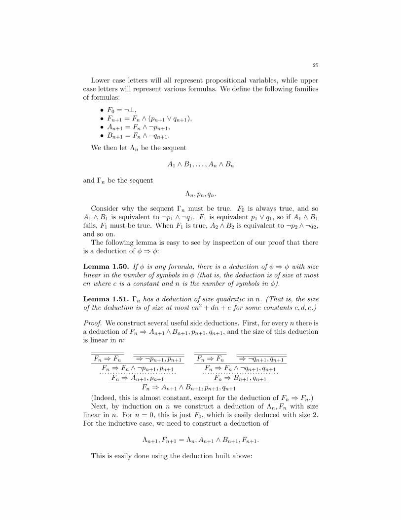
Lower case letters will all represent propositional variables, while uppercase letters will represent various formulas. We define the following familiesof formulas:

• F0 = ¬⊥,• Fn+1 = Fn ∧ (pn+1 ∨ qn+1),• An+1 = Fn ∧ ¬pn+1,• Bn+1 = Fn ∧ ¬qn+1.

We then let Λn be the sequent

A1 ∧B1, . . . , An ∧Bn

and Γn be the sequent

Λn, pn, qn.

Consider why the sequent Γn must be true. F0 is always true, and soA1 ∧ B1 is equivalent to ¬p1 ∧ ¬q1. F1 is equivalent p1 ∨ q1, so if A1 ∧ B1

fails, F1 must be true. When F1 is true, A2 ∧B2 is equivalent to ¬p2 ∧¬q2,and so on.

The following lemma is easy to see by inspection of our proof that thereis a deduction of φ⇒ φ:

Lemma 1.50. If φ is any formula, there is a deduction of φ⇒ φ with sizelinear in the number of symbols in φ (that is, the deduction is of size at mostcn where c is a constant and n is the number of symbols in φ).

Lemma 1.51. Γn has a deduction of size quadratic in n. (That is, the sizeof the deduction is of size at most cn2 + dn+ e for some constants c, d, e.)

Proof. We construct several useful side deductions. First, for every n there isa deduction of Fn ⇒ An+1∧Bn+1, pn+1, qn+1, and the size of this deductionis linear in n:

Fn ⇒ Fn ⇒ ¬pn+1, pn+1

Fn ⇒ Fn ∧ ¬pn+1, pn+1. . . . . . . . . . . . . . . . . . . . . . . . . . . . .Fn ⇒ An+1, pn+1

Fn ⇒ Fn ⇒ ¬qn+1, qn+1

Fn ⇒ Fn ∧ ¬qn+1, qn+1. . . . . . . . . . . . . . . . . . . . . . . . . . . . .Fn ⇒ Bn+1, qn+1

Fn ⇒ An+1 ∧Bn+1, pn+1, qn+1

(Indeed, this is almost constant, except for the deduction of Fn ⇒ Fn.)Next, by induction on n we construct a deduction of Λn, Fn with size

linear in n. For n = 0, this is just F0, which is easily deduced with size 2.For the inductive case, we need to construct a deduction of

Λn+1, Fn+1 = Λn, An+1 ∧Bn+1, Fn+1.

This is easily done using the deduction built above:

26

Λn, Fn

Fn ⇒ Fn

Fn ⇒ An+1 ∧Bn+1, pn+1, qn+1

Fn ⇒ An+1 ∧Bn+1, pn+1 ∨ qn+1

Fn ⇒ An+1 ∧Bn+1, Fn ∧ (pn+1 ∨ qn+1).. . . . . . . . . . . . . . . . . . . . . . . . . . . . . . . . . . . . . . . . . . . . . . .

Fn ⇒ An+1 ∧Bn+1,Fn+1

Λn, An+1 ∧Bn+1, Fn+1

From our deduction Λn, Fn, we wish to find a deduction of Γn+1 =Λn, An+1 ∧ Bn+1, pn+1, qn+1. This is given by applying cut to the deduc-tion of Λn, Fn and the deduction of Fn ⇒ An+1 ∧ Bn+1, pn+1, qn+1 givenabove.

�

We need the following lemma:

Lemma 1.52. Suppose there is a cut-free deduction of

Γn \ {Ai ∧Bi},¬pi, An+1 ∧Bn+1, pn+1, qn+1

for some i ≤ n. Then there is a cut-free deduction of Γn of the same size.

Proof. Since the deduction is cut-free, only the listed formulas can appear.We define an ad hoc transformation ·∗ on formulas appearing in this deduc-tion:

• p∗i is ⊥,• ¬p∗i is ⊥,• q∗i is ⊥,• For any other atomic formula or negation of an atomic formula p, p∗

is p,• (pi ∨ qi)∗ is ⊥,• For any other disjunction, φ∗ is φ,• For k < i, F ∗k is Fk,• F ∗i is Fi−1,• F ∗k+1 is F ∗k ∧ (pk ∨ qk) for k > i,• A∗k is F ∗k−1 ∧ ¬pk for k 6= i,• B∗k is F ∗k−1 ∧ ¬qk for k 6= i,• (Ak ∧Bk)∗ is A∗k ∧B∗k.

Let d be a deduction of a sequent ∆ ⇒ Σ consisting of subformulasof Γn \ {Ai ∧ Bi},¬pi, An+1 ∧ Bn+1, pn+1, qn+1 and with the property thatpi ∨ qi, pi, and qi do not appear except as subformulas of Fi. (In particular,do not appear themselves.) Let m be the size of d. We show by inductionon d that there is a cut-free deduction of ∆∗ ⇒ Σ∗ of size ≤ m.

Any axiom must be introducing some atomic formula which is unchanged,and so the axiom remains valid.

Suppose d consists of an introduction rule with main formula Fi; then oneof the subbranches contains a deduction of F ∗i = Fi−1, so we simply takethe result of IH applied to this subdeduction. (Note that pi ∨ qi, pi, and qi

27

may appear above the other branch, which we have just discarded, and sodo not need to apply IH to it.)

The only other inference rules which can appear are R→,R∧,R∨ appliedto formulas with the property that (φ~ψ)∗ = φ∗~ψ∗, and therefore remainvalid, so the claim in those cases followed immediately from IH.

In particular, we began with a deduction of

A1 ∧B1, . . . , Ai−1 ∧Bi−1, Ai+1 ∧Bi+1, . . . , An+1 ∧Bn+1,¬pi, pn+1, qn+1.

After the transformation, this becomes a deduction of

A1 ∧B1, . . . , Ai−1 ∧Bi−1, A∗i+1 ∧B∗i+1, . . . , A

∗n+1 ∧B∗n+1,⊥, pn+1, qn+1.

Applying inversion to eliminate ⊥ and renaming the propositional variablespk+1 to pk and qk+1 to qk for k ≥ i, we obtain a deduction of Γn. �

Theorem 1.53. A cut-free deduction of Γn has size ≥ 2n for all n ≥ 1.

Proof. By induction on n.Γ1 is the sequent A1 ∧ B1, p1, q1. This is not an axiom, and so has size

≥ 2.Suppose the claim holds for Γn. We show that it holds for Γn+1. The

only possible final rule in a cut-free deduction is R∧. We consider two cases.In the first case, the final rule introduces An+1 ∧ Bn+1. We thus have a

deduction of Λn, An+1, An+1 ∧ Bn+1, pn+1, qn+1 of size m and a deductionof Λn, Bn+1, An+1 ∧Bn+1, pn+1, qn+1 of size m′, with m+m′ + 1 the size ofthe whole deduction.

We work with the first of these deductions. Applying inversion twice, wehave a deduction of

Λn, Fn, pn+1, qn+1

of at most size m. Note that pn+1, qn+1 do not appear elsewhere in Λn, Fn.In particular, since pn+1, qn+1 do not appear negatively, there can be noaxiom rule for these variables anywhere in the deduction. Therefore wehave a deduction of

Λn, Fn = Λn, Fn−1 ∧ (pn ∨ qn)

of size at most m. Another application of inversion tells us that there mustbe a deduction of

Λn, pn, qn

of size at most m. But this is actually Γn, and therefore 2n ≤ m. The sameargument applied to the second of these deductions shows that 2n ≤ m′.Then the size of the deduction of Γn+1 wasm+m′+1 ≥ 2n+2n+1 = 2n+1+1.

In the second case, we must introduce Ai ∧ Bi for some i ≤ n. We thushave a deduction of Λn, Ai, An+1 ∧ Bn+1, pn+1, qn+1 of size m, a deductionof Λn, Bi, An+1∧Bn+1, pn+1, qn+1 of size m′, with m+m′+ 1 the size of thewhole deduction.

Applying inversion to the first of these gives a deduction of

Λn \ {Ai ∧Bi},¬pi, An+1 ∧Bn+1, pn+1, qn+1

28

of height at most m. By the previous lemma, it follows that there is adeduction of Γn of height at most m. By similar reasoning, there must be adeduction of Γn of height at most m′, and so again m+m′+1 ≥ 2n+1+1. �