Propositional Logic and Its Applications in ArtificialIntelligence

Jussi RintanenDepartment of Computer Science

Aalto UniversityHelsinki, Finland

April 5, 2017

Contents

Table of Contents . . . . . . . . . . . . . . . . . . . . . . . . . . . . . . . . . . . . . . . . . . . . . . i

1 Introduction 1

2 Definition 22.1 Formulas . . . . . . . . . . . . . . . . . . . . . . . . . . . . . . . . . . . . . . . . . . . . . . . 22.2 Equivalences . . . . . . . . . . . . . . . . . . . . . . . . . . . . . . . . . . . . . . . . . . . . . 32.3 Truth-tables . . . . . . . . . . . . . . . . . . . . . . . . . . . . . . . . . . . . . . . . . . . . . . 32.4 Logical Consequence, Satisfiability, Validity . . . . . . . . . . . . . . . . . . . . . . . . . . . . . 52.5 Normal Forms . . . . . . . . . . . . . . . . . . . . . . . . . . . . . . . . . . . . . . . . . . . . . 6

3 Automated Reasoning in the Propositional Logic 93.1 Truth-Tables . . . . . . . . . . . . . . . . . . . . . . . . . . . . . . . . . . . . . . . . . . . . . . 93.2 Tree-Search Algorithms . . . . . . . . . . . . . . . . . . . . . . . . . . . . . . . . . . . . . . . . 10

3.2.1 Unit Resolution . . . . . . . . . . . . . . . . . . . . . . . . . . . . . . . . . . . . . . . . 113.2.2 Subsumption . . . . . . . . . . . . . . . . . . . . . . . . . . . . . . . . . . . . . . . . . 123.2.3 Unit Propagation . . . . . . . . . . . . . . . . . . . . . . . . . . . . . . . . . . . . . . . 123.2.4 The Davis-Putnam Procedure . . . . . . . . . . . . . . . . . . . . . . . . . . . . . . . . 12

4 Applications 144.1 State-Space Search . . . . . . . . . . . . . . . . . . . . . . . . . . . . . . . . . . . . . . . . . . 14

4.1.1 Representation of Sets . . . . . . . . . . . . . . . . . . . . . . . . . . . . . . . . . . . . 144.1.2 Set Operations as Logical Operations . . . . . . . . . . . . . . . . . . . . . . . . . . . . 154.1.3 Relations as Formulas . . . . . . . . . . . . . . . . . . . . . . . . . . . . . . . . . . . . 154.1.4 Mapping from Actions to Formulas . . . . . . . . . . . . . . . . . . . . . . . . . . . . . 174.1.5 Finding Action Sequences through Satisfiability . . . . . . . . . . . . . . . . . . . . . . . 204.1.6 Relation Operations in Logic . . . . . . . . . . . . . . . . . . . . . . . . . . . . . . . . . 204.1.7 Symbolic State-Space Search . . . . . . . . . . . . . . . . . . . . . . . . . . . . . . . . 22

Index 24

i

Chapter 1

Introduction

The classical propositional logic is the most basic and most widely used logic. It is a notation for Booleanfunctions, together with several powerful proof and reasoning methods.

The use of the propositional logic has dramatically increased since the development of powerful search algo-rithms and implementation methods since the later 1990ies. Today the logic enjoys extensive use in several areasof computer science, especially in Computer-Aided Verification and Artificial Intelligence. Its uses in AI includeplanning, problem-solving, intelligent control, and diagnosis.

The reason why logics are used is their ability to precisely express data and information, in particular when theinformation is partial or incomplete, and some of the implicit consequences of the information must be inferredto make them explicit.

The propositional logic, as the first known NP-complete problem [Coo71], is used for representing many typesof co-NP-complete and NP-complete combinatorial search problems. Such problems are prevalent in artificialintelligence as a part of decision-making, problem-solving, planning, and other hard problems.

For many applications equally or even more natural choices would be various more expressive logics, includ-ing the predicate logic or various modal logics. These logics, however, lack the kind of efficient and scalablealgorithms that are available for the classical propositional logic. The existence of high performance algorithmsfor reasoning with propositional logic is the main reason for its wide use in computer science.

1

Chapter 2

Definition

2.1 Formulas

Propositional logic is about Boolean functions, which are mappings from truth-values 0 and 1 (false and true) totruth-values. Arbitrary Boolean functions can be represented as formulas formed with connectives such as ∧, ∨and ¬, and it can be shown that any Boolean function can be represented by such a formula.

Boolean functions and formulas have important applications in several areas of Computer Science.

• Digital electronics and the construction of digital computation devices such as microprocessors, is based onBoolean functions.

• The theory of computation and complexity uses Boolean functions for representing abstract models ofcomputation (for example Boolean circuits) and investigating their properties (for example the theory ofComputational Complexity, where some of the fundamental results like NP-completeness [Coo71, GJ79]were first established with Boolean functions).

• Parts of Artificial Intelligence use Boolean functions and formulas for representing models of the world andthe reasoning processes of intelligent systems.

The most primitive Boolean functions are represented by the connectives ∨, ∧, ¬,→ and↔ as follows.

α β α ∨ β0 0 0

0 1 1

1 0 1

1 1 1

α β α ∧ β0 0 0

0 1 0

1 0 0

1 1 1

α ¬α0 1

1 0

α β α→ β

0 0 1

0 1 1

1 0 0

1 1 1

α β α↔ β

0 0 1

0 1 0

1 0 0

1 1 1

The connectives are used for forming complex Boolean functions from primitive ones.Often only some of the connectives, typically ¬ and one or both of ∧ and ∨ are viewed as the primitive

connectives, and other connectives are defined in terms of the primitive connectives. The implication → andequivalence↔ connectives are often viewed as non-primitive: α→ β can be defined as ¬α ∨ β, and α↔ β canbe defined as (α→ β) ∧ (β → α).

There is a close connection between the Boolean connectives ∨, ∧ and ¬ and the operations ∪, ∩ and com-plementation in Set Theory. Observe the similarity between the truth-tables for the three connectives and theanalogous tables for the set-theoretic operations.

α β α ∪ β∅ ∅ ∅∅ {1} {1}{1} ∅ {1}{1} {1} {1}

α β α ∩ β∅ ∅ ∅∅ {1} ∅{1} ∅ ∅{1} {1} {1}

α α

∅ {1}{1} ∅

Formed analogously to expressions in mathematics (parentheses, +, × etc.)

Definition 2.1 (Propositional Formulas) Formulas a recursively defined as follows.

2

2.2. EQUIVALENCES 3

• Atomic propositions x ∈ X are formulas.

• Symbols > and ⊥ are formulas.

• If α and β are formulas, then so are

1. ¬α2. (α ∧ β)

3. (α ∨ β)

4. (α→ β)

5. (α↔ β)

Nothing else is a formula.

Parentheses ( and ) do not always need to be written if precedences between the connectives are observed. Thehighest precedence is with ¬, followed by ∧ and ∨, then→, and finally↔.

Definition 2.2 (Valuation of atomic propositions) A valuation v : X → {0, 1} is a mapping from atomic propo-sitions X = {x1, . . . , xn} to truth-values 0 and 1.

Valuations can be extended to formulas φ ∈ L, i.e. v : L → {0, 1}.

Definition 2.3 (Valuation of propositional formulas) A given valuation v : X → {0, 1} of atomic propositionscan be extended to a valuation of arbitrary propositional formulas over X .

v(¬α) = 1 iff v(α) = 0v(>) = 1v(⊥) = 0v(α ∧ β) = 1 iff v(α) = 1 and v(β) = 1v(α ∨ β) = 1 iff v(α) = 1 or v(β) = 1v(α→ β) = 1 iff v(α) = 0 or v(β) = 1v(α↔ β) = 1 iff v(α) = v(β)

Example 2.4 Let v(a) = 1, v(b) = 1, v(c) = 1, v(d) = 1

v(a ∨ b ∨ c) = 1v(¬a→ b) = 1v(a→ ¬b) = 0

�

2.2 Equivalences

Table 2.1 lists equivalences that hold in the propositional logic. Replacing one side of any of these equivalencesby the other - in any formula - does not change the Boolean function represented by the formula.

These equivalences have several applications, including translating formulas into normal forms (Section 2.5),and simplifying formulas. For example, all occurrences> and⊥ of the constant symbols (except one, if the wholeformula reduces to > or ⊥) can be eliminated with the equivalences containing these symbols.

2.3 Truth-tables

All valuations relevant to a formula are often tabulated as truth-tables so that each row corresponds to a valuation.Truth-tables are used for analyzing the most basic properties of formulas.

Valuations for formulas containing exactly one connective are as follows.

4 CHAPTER 2. DEFINITION

double negation ¬¬α ≡ αassociativity ∨ α ∨ (β ∨ γ) ≡ (α ∨ β) ∨ γassociativity ∧ α ∧ (β ∧ γ) ≡ (α ∧ β) ∧ γcommutativity ∨ α ∨ β ≡ β ∨ αcommutativity ∧ α ∧ β ≡ β ∧ αdistributivity ∧ ∨ α ∧ (β ∨ γ) ≡ (α ∧ β) ∨ (α ∧ γ)distributivity ∨ ∧ α ∨ (β ∧ γ) ≡ (α ∨ β) ∧ (α ∨ γ)idempotence ∨ α ∨ α ≡ αidempotence ∧ α ∧ α ≡ αabsorption 1 α ∧ (α ∨ β) ≡ αabsorption 2 α ∨ (α ∧ β) ≡ αDe Morgan’s law 1 ¬(α ∨ β) ≡ (¬α) ∧ (¬β)De Morgan’s law 2 ¬(α ∧ β) ≡ (¬α) ∨ (¬β)contraposition α→ β ≡ ¬β → ¬αnegation > ¬> ≡ ⊥negation ⊥ ¬⊥ ≡ >constant ⊥ α ∧ ¬α ≡ ⊥constant > α ∨ ¬α ≡ >elimination > ∨ > ∨ α ≡ >elimination > ∧ > ∧ α ≡ αelimination ⊥ ∨ ⊥ ∨ α ≡ αelimination ⊥ ∧ ⊥ ∧ α ≡ ⊥elimination ⊥→ ⊥ → α ≡ >elimination ⊥→ α→ ⊥ ≡ ¬αelimination >→ > → α ≡ αelimination >→ α→ > ≡ >commutativity↔ α↔ β ≡ β ↔ αelimination >↔ > ↔ α ≡ αelimination ⊥↔ ⊥ ↔ α ≡ ¬α

Table 2.1: Propositional Equivalences

2.4. LOGICAL CONSEQUENCE, SATISFIABILITY, VALIDITY 5

α ∧ β |= αα |= α ∨ βα |= β → α¬α |= α→ β

α ∧ (α→ β) |= β¬β ∧ (α→ β) |= ¬α

Table 2.2: Useful Logical Consequences

α ¬α0 11 0

α β α ∧ β0 0 00 1 01 0 01 1 1

α β α ∨ β0 0 00 1 11 0 11 1 1

α β α→ β

0 0 10 1 11 0 01 1 1

α β α↔ β

0 0 10 1 01 0 01 1 1

1. Columns for all n atomic propositions in the formula

2. Columns for all subformulas of the formula

3. Write 2n rows corresponding to the valuations

4. Fill in truth-values in the remaining cells

Example 2.5 The truth-table for ¬B ∧ (A→ B) is

A B ¬B (A→ B) (¬B ∧ (A→ B))

0 0 1 1 10 1 0 1 01 0 1 0 01 1 0 1 0

�

2.4 Logical Consequence, Satisfiability, Validity

Definition 2.6 (Logical Consequence) A formula φ is a logical consequence of Σ = {φ1, . . . , φn}, denoted byΣ |= φ, if and only if for all valuations v, if v |= Σ then v |= φ.

Logical consequences are what can be inferred with certainty.

Example 2.7 From “if it is a weekday today then most people are working today”, and “it is a weekday today” itfollows that “most people are working today”.{w → p, w} |= p �

Example 2.8 {a, a→ b, b→ c} |= c �

Example 2.9 {m ∨ t,m→ w, t→ w} |= w �

Definition 2.10 (Validity) A formula φ is valid if and only if v(φ) = 1 for all valuations v.

Example 2.11 x ∨ ¬x is valid.x→ (x ∨ y) is valid.x ∨ y is not valid. �

6 CHAPTER 2. DEFINITION

Definition 2.12 (Satisfiability) A formula φ is satisfiable if and only if there is at least one valuation v such thatv(φ) = 1.

A set {φ1, . . . , φn} is satisfiable if there is at least one valuation v such that v(φi) = 1 for all i ∈ {1, . . . , n}.

Example 2.13 The following formulas are satisfiable: x, x ∧ y, and x ∨ ¬x. �

Example 2.14 The following formulas are not satisfiable: x ∧ ¬x, ⊥, a ∧ (a→ b) ∧ ¬b. �

A satisfiable formula is also said to be consistent. A formula that is not satisfiable is unsatisfiable, inconsistent,or contradictory.

Satisfiability means logically possible: it is possible that the formula is true (if the truth-values of the atomicpropositions in the formula are chosen right.)

Interestingly, there are close connections between satisfiability, validity, and logical consequence. These con-nections allow reducing questions concerning these concepts to each other, which allows choosing one of theseconcepts as the most basic one (for example implemented in algorithms for reasoning in the propositional logic),and reducing the other concepts to the basic one.

Theorem 2.15 (Validity vs. Logical Consequence 1) φ is valid if and only if ∅ |= φ

Theorem 2.16 (Validity vs. Logical Consequence 2) {φ1, . . . , φn} |= φ if and only if (φ1 ∧ · · · ∧ φn) → φ isvalid.

Theorem 2.17 (Satisfiability vs. Validity) φ is satisfiable if and only if ¬φ is not valid.

Theorem 2.18 (Logical Consequence vs. Satisfiability) Σ |= φ if and only if Σ ∪ {¬φ} is not satisfiable.

In practice, algorithms for the propositional logic implement satisfiability. Other reasoning tasks are reducedto satisfiability testing.

Example 2.19 {m∨ t,m→ w, t→ w} |= w if and only if (m∨ t)∧ (m→ w)∧ (t→ w)∧¬w is not satisfiable.�

2.5 Normal Forms

Arbitrary propositional formulas can be translated to syntactically restricted forms. This can serve two mainpurposes. First, it may be more straightforward to define algorithms and inference methods when the formulasare in certain simple forms. The resolution rule (Section 3.2.1) is an example of this. Second, the process oftranslating a formula into a normal form does much of the work in solving important computational problemsrelated to propositional formulas. For example, an answer to the question of whether a formula is valid is obtainedas a by-product of translating the formula into certain normal forms.

In this course we focus on the best known normal form which is the conjunctive normal form.

Definition 2.20 (Literals) If x is an atomic proposition, then x and ¬x are literals.

Definition 2.21 (Clauses) If l1, . . . , ln are literals, then l1 ∨ · · · ∨ ln is a clause.

Definition 2.22 (Terms) If l1, . . . , ln are literals, then l1 ∧ · · · ∧ ln is a term.

Definition 2.23 (Conjunctive Normal Form) If φ1, . . . , φm are clauses, then the formula φ1 ∧ · · · ∧ φm is inconjunctive normal form.

Example 2.24 The following formulas are in conjunctive normal form.

¬x¬x1 ∨ ¬x2

x3 ∧ x4

(¬x1 ∨ ¬x2) ∧ ¬x3 ∧ (x4 ∨ ¬x5)

�

2.5. NORMAL FORMS 7

α↔ β (¬α ∨ β) ∧ (¬β ∨ α) (2.1)

α→ β ¬α ∨ β (2.2)

¬(α ∨ β) ¬α ∧ ¬β (2.3)

¬(α ∧ β) ¬α ∨ ¬β (2.4)

¬¬α α (2.5)

α ∨ (β ∧ γ) (α ∨ β) ∧ (α ∨ γ) (2.6)

(α ∧ β) ∨ γ (α ∨ γ) ∧ (β ∨ γ) (2.7)

Table 2.3: Rewriting Rules for Translating Formulas to Conjunctive Normal Form

Table 2.3 lists rules that transform any formula into CNF. These rules are instances of the equivalence listed inTable 2.1

Algorithm 2.25 Any formula can be translated into conjunctive normal form as follows.

1. Eliminate connective↔ (Rule 2.1).

2. Eliminate connective→ (Rule 2.2).

3. Move ¬ inside ∨ and ∧ (Rules 2.3 and 2.4).

4. Move ∧ outside ∨ (Rules 2.6 and 2.7).

Notice that the last step of the transformation multiplies the number of copies of subformulas α and γ. Forsome classes of formulas this transformation therefore leads to exponentially big normal forms.

Formulas in CNF are often represented as sets of clauses, with clauses represented as sets of literals. Theplacement of connectives ∨ and ∧ can be left implicit because of the simple structure of CNF. The CNF (A∨B ∨C) ∧ (¬A ∨D) ∧ E is represented as {A ∨B ∨ C, ¬A ∨D, E}.

Example 2.26 Translate A ∨B → (B ↔ C) into CNF. A ∨B → (B → C) ∧ (C → B) ¬(A ∨B) ∨ ((¬B ∨ C) ∧ (¬C ∨B)) (¬A ∧ ¬B) ∨ ((¬B ∨ C) ∧ (¬C ∨B)) (¬A ∨ ((¬B ∨ C) ∧ (¬C ∨B)))∧ (¬B ∨ ((¬B ∨ C) ∧ (¬C ∨B))) (¬A ∨ ¬B ∨ C) ∧ (¬A ∨ ¬C ∨B)∧ (¬B ∨ ((¬B ∨ C) ∧ (¬C ∨B))) (¬A ∨ ¬B ∨ C) ∧ (¬A ∨ ¬C ∨B)∧ (¬B ∨ ¬B ∨ C) ∧ (¬B ∨ ¬C ∨B)

�

Another often used normal form is the Disjunctive Normal Form (DNF).

Definition 2.27 (Disjunctive Normal Form) If φ1, . . . , φm are terms, then the formula φ1 ∨ · · · ∨ φm is in dis-junctive normal form.

Disjunctive normal forms are found with a procedure similar to that for CNF. The only difference is that adifferent set of distributivity rules is applied, for moving ∧ inside ∨ instead of the other way round.

A less restrictive normal form that includes both CNF and DNF is the Negation Normal Form (NNF). It isuseful in many types of automated processing of formulas because of its simplicity and the fact that translationinto NNF only minimally affects the size of a formula, unlike the translations into DNF and CNF which mayincrease the size exponentially.

Definition 2.28 (Negation Normal Form) Let X be a set of atomic propositions.

1. ⊥ and > are in negation normal form.

2. x and ¬x for any x ∈ X are in negation normal form.

8 CHAPTER 2. DEFINITION

3. φ1 ∧ φ2 is in negation normal form if φ1 and φ2 both are.

4. φ1 ∨ φ2 is in negation normal form if φ1 and φ2 both are.

No other formula is in negation normal form.

After performing the first three steps in the translation into CNF the formula is in NNF. Notice that only theapplication of the distributivity equivalences increases the number of atomic propositions in the CNF translation.The translation into NNF does not affect the number of occurrences of atomic propositions or the connectives ∨and ∧, and the size of the resulting formula can be bigger only because of the higher number of occurrences ofnegation symbols ¬. Hence the NNF is never more than twice as big as the original formula.

Chapter 3

Automated Reasoning in the PropositionalLogic

In this chapter we discuss the main methods for automating inference in the propositional logic.The simplest method is based on truth-tables (Section 3.1), which enumerate all valuations of the relevant

atomic propositions, and questions about satisfiability and logical consequence can be answered by evaluating thetruth-values of the relevant formulas for every valuation.

Truth-tables are easy to implement as a program, but are impractical when the number of atomic propositionsis higher than 20 or 30. The algorithms used in practice (Section 3.2) are based on searching a tree in which eachpath starting from the root node represents a (partial) valuation of the atomic propositions. The size of this tree isin practice orders of magnitudes smaller than corresponding truth-tables, and for finding one satisfying valuationnot the whole tree needs to be traversed. Finally, only one path of the tree, from the root node to the currentleaf node, needs to be kept in the memory at a time, which reduces the memory requirements substantially. Thisenables the use of these algorithms for formulas of the size encountered in solving important problems in AI andcomputer science in general, with up to hundreds of thousands of atomic propositions and millions of clauses.

3.1 Truth-Tables

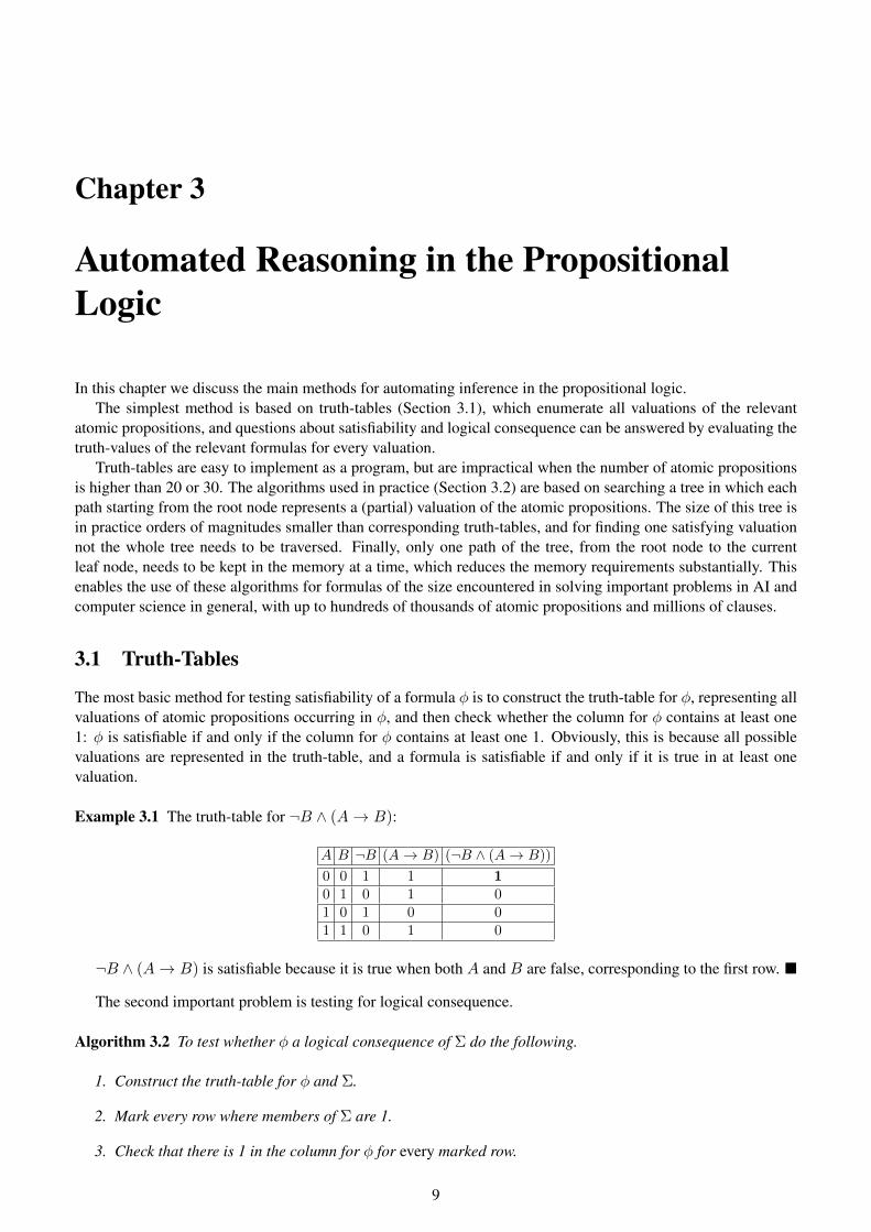
The most basic method for testing satisfiability of a formula φ is to construct the truth-table for φ, representing allvaluations of atomic propositions occurring in φ, and then check whether the column for φ contains at least one1: φ is satisfiable if and only if the column for φ contains at least one 1. Obviously, this is because all possiblevaluations are represented in the truth-table, and a formula is satisfiable if and only if it is true in at least onevaluation.

Example 3.1 The truth-table for ¬B ∧ (A→ B):

A B ¬B (A→ B) (¬B ∧ (A→ B))

0 0 1 1 10 1 0 1 01 0 1 0 01 1 0 1 0

¬B ∧ (A→ B) is satisfiable because it is true when both A and B are false, corresponding to the first row. �

The second important problem is testing for logical consequence.

Algorithm 3.2 To test whether φ a logical consequence of Σ do the following.

1. Construct the truth-table for φ and Σ.

2. Mark every row where members of Σ are 1.

3. Check that there is 1 in the column for φ for every marked row.

9

10 CHAPTER 3. AUTOMATED REASONING IN THE PROPOSITIONAL LOGIC

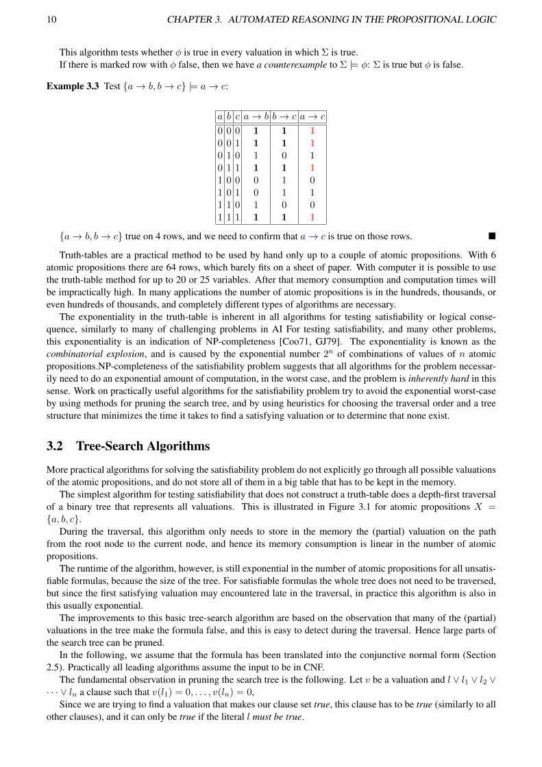
This algorithm tests whether φ is true in every valuation in which Σ is true.If there is marked row with φ false, then we have a counterexample to Σ |= φ: Σ is true but φ is false.

Example 3.3 Test {a→ b, b→ c} |= a→ c:

a b c a→ b b→ c a→ c

0 0 0 1 1 10 0 1 1 1 10 1 0 1 0 10 1 1 1 1 11 0 0 0 1 01 0 1 0 1 11 1 0 1 0 01 1 1 1 1 1

{a→ b, b→ c} true on 4 rows, and we need to confirm that a→ c is true on those rows. �

Truth-tables are a practical method to be used by hand only up to a couple of atomic propositions. With 6atomic propositions there are 64 rows, which barely fits on a sheet of paper. With computer it is possible to usethe truth-table method for up to 20 or 25 variables. After that memory consumption and computation times willbe impractically high. In many applications the number of atomic propositions is in the hundreds, thousands, oreven hundreds of thousands, and completely different types of algorithms are necessary.

The exponentiality in the truth-table is inherent in all algorithms for testing satisfiability or logical conse-quence, similarly to many of challenging problems in AI For testing satisfiability, and many other problems,this exponentiality is an indication of NP-completeness [Coo71, GJ79]. The exponentiality is known as thecombinatorial explosion, and is caused by the exponential number 2n of combinations of values of n atomicpropositions.NP-completeness of the satisfiability problem suggests that all algorithms for the problem necessar-ily need to do an exponential amount of computation, in the worst case, and the problem is inherently hard in thissense. Work on practically useful algorithms for the satisfiability problem try to avoid the exponential worst-caseby using methods for pruning the search tree, and by using heuristics for choosing the traversal order and a treestructure that minimizes the time it takes to find a satisfying valuation or to determine that none exist.

3.2 Tree-Search Algorithms

More practical algorithms for solving the satisfiability problem do not explicitly go through all possible valuationsof the atomic propositions, and do not store all of them in a big table that has to be kept in the memory.

The simplest algorithm for testing satisfiability that does not construct a truth-table does a depth-first traversalof a binary tree that represents all valuations. This is illustrated in Figure 3.1 for atomic propositions X ={a, b, c}.

During the traversal, this algorithm only needs to store in the memory the (partial) valuation on the pathfrom the root node to the current node, and hence its memory consumption is linear in the number of atomicpropositions.

The runtime of the algorithm, however, is still exponential in the number of atomic propositions for all unsatis-fiable formulas, because the size of the tree. For satisfiable formulas the whole tree does not need to be traversed,but since the first satisfying valuation may encountered late in the traversal, in practice this algorithm is also inthis usually exponential.

The improvements to this basic tree-search algorithm are based on the observation that many of the (partial)valuations in the tree make the formula false, and this is easy to detect during the traversal. Hence large parts ofthe search tree can be pruned.

In the following, we assume that the formula has been translated into the conjunctive normal form (Section2.5). Practically all leading algorithms assume the input to be in CNF.

The fundamental observation in pruning the search tree is the following. Let v be a valuation and l ∨ l1 ∨ l2 ∨· · · ∨ ln a clause such that v(l1) = 0, . . . , v(ln) = 0,

Since we are trying to find a valuation that makes our clause set true, this clause has to be true (similarly to allother clauses), and it can only be true if the literal l must be true.

3.2. TREE-SEARCH ALGORITHMS 11

a = 0a = 1

b = 0b = 1b = 0b = 1

c = 0c = 1c = 0c = 1 c = 0c = 1c = 0c = 1

Figure 3.1: All valuations as a binary tree

Hence if the partial valuation corresponding to the current node in the search tree makes, in some clause, allliterals false except one (call it l) that still does not have a truth-value, then l has to be made true. If l is an atomicpropositions x, then the current valuation has to assign v(x) = 1, and if l = ¬x for some atomic proposition x,then we have to assign v(x) = 0. We call these forced assignments.

Consider the search tree in Figure 3.1 and the clauses ¬a ∨ b and ¬b ∨ c. The leftmost child node of the rootnode, which is reached by following the arc a = 1, corresponds to the partial valuation v = {(a, 1)} that assignsv(a) = 1 and leaves the truth-values of the remaining atomic propositions open. Now with clause ¬a∨ b we havethe forced assignment v(b) = 1. Now, with clause ¬b ∨ c also v(c) = 1 is a forced assignment.

Hence assigning a = 1 forces the assignments of both of the remaining variables. This means that the leftmostsubtree of the root node essentially only consists of one path that leads to the leftmost leaf node. The other leafnodes in the tree, corresponding to valuations {a = 1, b = 1, c = 0}, {a = 1, b = 0, c = 1}, and {a = 1, b =0, c = 1}, would not be visited, because it is obvious that they falsify at least one of the clauses. Since we aredoing the tree search in order to determine the satisfiability of our clause set, the computation can be stopped here.The rightmost subtree of the root node, corresponding to all valuations with a = 0, is therefore not visited at all.

3.2.1 Unit Resolution

What we described as forced assignments is often formalized as the inference rule Unit Resolution.

Theorem 3.4 (Unit Resolution) Inl l ∨ l1 ∨ l2 ∨ · · · ∨ ln

l1 ∨ l2 ∨ · · · ∨ lnthe formula below the line is a logical consequence of the formulas above the line.

Here the complementation l of a literal l is defined by x = ¬x and ¬x = x.

Example 3.5 From {A ∨B ∨ C,¬B,¬C} one can derive A by two applications of the Unit Resolution rule. �

A special case of the Unit Resolution rule is when both clauses are unit clauses (consisting of one literal only.)Since the n = 0 in this case, the formula below the line has 0 disjuncts. We identify a chain-disjunction with 0literals with the constant false ⊥, corresponding to the empty clause.

l l

⊥Any clause set with the empty clause is unsatisfiable.The Unit Resolution rule is a special case of the Resolution rule (which we will not be discussing in more

detail.)

Theorem 3.6 (Resolution) Inl ∨ l′1 ∨ · · · ∨ l′m l ∨ l1 ∨ · · · ∨ lnl′1 ∨ · · · ∨ l′m ∨ l1 ∨ l2 ∨ · · · ∨ ln

the formula below the line is a logical consequence of the formulas above the line.

12 CHAPTER 3. AUTOMATED REASONING IN THE PROPOSITIONAL LOGIC

1: procedure DPLL(S)2: S := UP(S);3: if ⊥ ∈ S then return false;4: x := any atomic proposition such that {x,¬x} ∩ S = ∅;5: if no such x exists then return true;6: if DPLL(S ∪ {x}) then return true;7: return DPLL(S ∪ {¬x})

Figure 3.2: The DPLL procedure

3.2.2 Subsumption

If a clause set contains two clauses with literals {l1, . . . , ln} and {l1, . . . , ln, ln+1, . . . , lm}, respectively, then thelatter clause can be removed, as it is a logical consequence of the former, and hence both clause sets are true inexactly the same valuations.

Example 3.7 Applying the Subsumption rule to {A ∨B ∨ C,A ∨ C} yields the equivalent set {A ∨ C}. �

If the shorter clause is a unit clause, then this is called Unit Subsumption.

3.2.3 Unit Propagation

Performing all unit resolutions exhaustively leads to the Unit Propagation procedure, also known as BooleanConstraint Propagation (BCP).

In practice, when a clause l1 ∨ · · · ∨ ln with n > 2 can be resolved with a unit clause, the shorter clause oflength n − 1 > 1 is not produced. This would often lead to producing n − 1 clauses, of lengths 1, 2, . . . , n − 1.Practical implementation of the unit propagation procedure only produce a new clause when the complementsof all but 1 of the n literals of the clause have been inferred. This can be formalized as the following rule, withn ≥ 2.

l2 l3 . . . ln−1 l1 ∨ · · · ∨ lnln

We denote by UP(S) the clause set obtained by performing all possible unit propagations to a clause set S,followed by applying the subsumption rule.

3.2.4 The Davis-Putnam Procedure

The Davis-Putnam-Logemann-Loveland procedure (DPLL), often known as simply the Davis-Putnam procedure,is given in Figure 3.2.

We have sketched the algorithm so that the first branch assigns the chosen atomic proposition x true in thefirst subtree (line 6) and false in the second (line 7). However, these two branches can be traversed in eitherorder (exchanging x and ¬x on lines 6 and 7), and efficient implementations use this freedom by using powerfulheuristics for choosing first the atomic proposition (line 4) and then choosing its truth-value.

Theorem 3.8 Let S be a set of clauses. Then DPLL(S) returns true if and only if S is satisfiable.

References

Automation of reasoning in the classical propositional logic started in the works of Davis and Putnam and theirco-workers, resulting in the Davis-Putnam-Logemann-Loveland procedure [DLL62] (earlier known as the Davis-Putnam procedure ) and other procedures [DP60].

Efforts to implement the Davis-Putnam procedure efficiently lead to fast progress from mid-1990ies on.The current generation of solvers for solving the SAT problem are mostly based on the Conflict-Driven Clause

Learning procedure which emerged from the work of Marques-Silva and Sakallah [MSS96]. Many of the currentleading implementation techniques and heuristics for selecting the decision variables come from the work onthe Chaff solver [MMZ+01]. Several other recent developments have strongly contributed to current solvers[PD07, AS09].

3.2. TREE-SEARCH ALGORITHMS 13

Unit propagation can be implemented to run in linear time in the size of the clause set, which in the simplestvariants involve updating a counter every time a literal in a clause gets a truth-value [DG84]. Modern SATsolvers attempt to minimize memory accesses (cache misses), and even counter-based linear time procedures areconsidered too expensive, and unit propagation schemes that do not use counters are currently used [MMZ+01].

Also stochastic local search algorithms have been used for solving the satisfiability problem [SLM92], but theyare not used in many applications because of their inability to detect unsatisfiability.

The algorithms in this chapter assumed the formulas to be in CNF. As discussed in Section 2.5, the translationto CNF may in some cases exponentially increase the size of the formula. However, for the purposes of satisfi-ability testing, there are transformations to CNF that are of linear size and preserve satisfiability (but not logicalequivalence.) These transformations are used for formulas that are not already in CNF [Tse68, CMV09].

Chapter 4

Applications

4.1 State-Space Search

State-space search is the problem of testing whether a state in a transition system is reachable from one or moreinitial states. Transition systems in the most basic cases can be identified with graphs, and the state-space searchproblem in this case is the s-t-reachability problem in graphs.

For small graphs the problem can be solved with standard graph search algorithms such as Dijkstra’s algorithm.For graphs with an astronomically high number of states, 1010 or more, standard graph algorithms are impractical.Many transition systems can be compactly represented, yet their size as graphs is very high. This is becauseN Boolean (0-1) state variables together with a state-variable based representation of the possible actions orevents can induce a state-space with the order of 2n reachable states. This is often known as the combinatorialexplosion. It turns out that the s-t-reachability problem for natural compactly represented graphs is PSPACE-complete [GW83, Loz88, LB90, Byl94].

Classical propositional logic has been proposed as one solution to state-space search problems for very largegraphs, due to the possibility of representing and reasoning about large numbers of states with (relatively small)formulas.

4.1.1 Representation of Sets

A state in a transition system is an assignment of values to the state variables. In this work we restrict to finite-valued state variables. Without loss of generality we will limit to Boolean (two-valued, 0-1) state variables,because any n-valued state variables can be represented in terms of dlog2 ne Boolean state variables.

We will be representing states with n Boolean state-variables as n-bit bit-vectors.

Example 4.1 Let X = {A,B,C,D}. Now a valuation that assigns 1 to A and C corresponds to the bit-vectorA1B0C1D0 , and the valuation assigning 1 only to B corresponds to the bit-vector

A0B1C0D0 . �

Any propositional formula φ can be understood as a representation of those valuations v such that v(φ) = 1.Since we have identified valuations and bit-vectors and states, a formula naturally represents a set of states orbit-vectors.

Example 4.2 Formula B represents all bit-vectors of the form ?1??, and the formula A represents all bit-vectors1???. Formula B therefore represents the set

{0100, 0101, 0110, 0111, 1100, 1101, 1110, 1111}

and formula A represents the set

{1000,1001,1010,1011,1100,1101,1110,1111}.

�

Similarly, ¬B represents all bit-vectors of the form ?0??, which is the set

{0000, 0001, 0010, 0011, 1000, 1001, 1010, 1011}.

This is the complement of the set represented by B.

14

4.1. STATE-SPACE SEARCH 15

state sets formulas over Xthose 2|X|

2 bit-vectors where x is true x ∈ XE (complement) ¬EE ∪ F E ∨ FE ∩ F E ∧ FE\F (set difference) E ∧ ¬F

the empty set ∅ ⊥ (constant false)the universal set > (constant true)

question about sets question about formulasE ⊆ F ? E |= F ?E ⊂ F ? E |= F and F 6|= E?E = F ? E |= F and F |= E?

Table 4.1: Connections between Set-Theory and Propositional Logic

4.1.2 Set Operations as Logical Operations

There is a close connection between the Boolean connectives ∨, ∧, ¬ and the set-theoretical operations of union,intersection and complementation, which is also historically the origin of Boole’s work on Boolean functions.

If φ1 and φ2 represent bit-vector sets S1 and S2, then

1. φ1 ∧ φ2 represents set S1 ∩ S2,

2. φ1 ∨ φ2 represents set S1 ∪ S2, and

3. ¬φ1 represents set S1.

Example 4.3 A∧B represents the set {1100, 1101, 1110, 1111} andA∨B represents the set {0100, 0101, 0110,0111, 1000, 1001, 1010, 1011, 1100, 1101, 1110, 1111}. �

Questions about the relations between sets represented as formulas can be reduced to the basic logical conceptswe already know, namely logical consequence, satisfiability, and validity.

1. “Is φ satisfiable?” corresponds to “Is the set represented by φ non-empty?”

2. φ |= α corresponds to “Is the set represented by φ a subset of the set represented by α?”.

3. “Is φ valid?” corresponds to “Is the set represented by φ the universal set?”

These connections allow using propositional formulas as a data structure in some applications in which con-ventional enumerative data structures for sets are not suitable because of the astronomic number of states. Forexample, if there are 100 state variables, then any formula consisting of just one atomic proposition represents aset of 299 = 633825300114114700748351602688 bit-vectors, which would require 7493989779944505344 TBin an explicit enumerative representation if each of the 100-bit vectors was represented with 13 bytes (wastingonly 4 bits in the 13th byte.)

4.1.3 Relations as Formulas

Similarly to finite sets of atomic objects, relations on any finite set of objects can be represented as propositionalformulas.

A binary relation R ⊆ X×X is a set of pairs (a, b) ∈ X×X , and the representation of this relation is similarto representing sets before, except that the elements are pairs.

As before, we assume that the atomic objects are bit-vectors. A pair of bit-vectors of lengths n and m can ofcourse be represented as a bit-vector of length n+m, simply by attaching the two bit-vectors together.

16 CHAPTER 4. APPLICATIONS

000

001010

011

100

101110

111

Figure 4.1: Transition relation as a graph

Example 4.4 To represent the pair (0001, 1100) of bit-vectors, both expressed as valuations of atomic propo-sitions A,B,C,D, instead use the atomic propositions X01 = {A0, B0, C0, D0, A1, B1, C1, D1} as the indexvariables, instead of X = {A,B,C,D}.

The pair (0001, 1100) is hence represented as 00011100, a valuation of X01. �

Pair (A0

0B0

0C0

0D0

1 ,A1

1B1

1C1

0D1

0 ) therefore corresponds to the valuation that assigns 1 to D0, A1 and B1 and 0 to allother variables.

Example 4.5 (A0 ↔ A1) ∧ (B0 ↔ B1) ∧ (C0 ↔ C1) ∧ (D0 ↔ D1) represents the identity relation of 4-bitbit-vectors. �

Example 4.6 The formula

inc01 = (¬C0 ∧ C1 ∧ (B0 ↔ B1) ∧ (A0 ↔ A1))∨(¬B0 ∧ C0 ∧B1 ∧ ¬C1 ∧ (A0 ↔ A1))∨(¬A0 ∧B0 ∧ C0 ∧A1 ∧ ¬B1 ∧ ¬C1)∨(A0 ∧B0 ∧ C0 ∧ ¬A1 ∧ ¬B1 ∧ ¬C1)

represents the successor relation of 3-bit integers

{(000, 001), (001, 010), (010, 011), (011, 100), (100, 101), (101, 110), (110, 111), (111, 000)}.

�

Example 4.7 Consider the transition relation {(001, 111), (010, 110), (011, 010), (111, 110)} corresponding tothe graph in Figure 4.1 The relation can be represented as the following truth-table (listing only those of the26 = 64 lines that have 1 in the column for φ.)

a0 b0 c0 a1 b1 c1 φ...0 0 1 1 1 1 1...0 1 0 1 1 0 1...0 1 1 0 1 0 1...1 1 1 1 1 0 1...

4.1. STATE-SPACE SEARCH 17

which is equivalent to the following formula.

(¬a0 ∧ ¬b0 ∧ c0 ∧ a1 ∧ b1 ∧ c1)∨(¬a0 ∧ b0 ∧ ¬c0 ∧ a1 ∧ b1 ∧ ¬c1)∨(¬a0 ∧ b0 ∧ c0 ∧ ¬a1 ∧ b1 ∧ ¬c1)∨(a0 ∧ b0 ∧ c0 ∧ a1 ∧ b1 ∧ ¬c1)

�

Any binary relation (transition relation) over a finite set can be represented as a propositional formula in thisway. These formulas can be used as components of formulas that represent paths in the graphs corresponding tothe binary relation.

Given a formula for the binary relation (corresponding to edges of the graphs), a formula for any path of agiven length T can be obtained by making T copies of the formula and renaming the atomic propositions for thestate variables.

Example 4.8 Consider the increment relation from Example 4.6 and the corresponding formula inc01. We makethree copies of inc01 and change the subscripts of the variables in the last two copies by adding 1 and 2 to them,respectively.

inc01 ∧ inc12 ∧ inc23 ∧ inc34.

The valuations that satisfy this formula exactly correspond to the sequences s0, s1, s2, s3, s4 of consecutivenodes/states in the graph with edges represented by inc01. �

Example 4.9 Can bit-vector 100 be reached from bit-vector 000 by four steps?This is equivalent to the satisfiability of the following formula.

¬A0 ∧ ¬B0 ∧ ¬C0 ∧ inc01 ∧ inc12 ∧ inc23 ∧ inc34 ∧A4 ∧ ¬B4 ∧ ¬C4

This formula represent the subset of the set of sequences s0, s1, s2, s3, s4 that start from the state/node s0 suchthat s0 |= ¬A ∧ ¬B ∧ ¬C is true and ends in the state s4 such that s4 |= A ∧ ¬B ∧ ¬C. �

For most applications of state-space search there are nodes/states that have multiple successor nodes. This isbecause the event that may take place in the state is non-deterministic, or because the agent whose behavior wehave modeled can take more than one alternative action in that state.

Consider the action that multiplies a 3-bit binary number by 2, which shifts all bits one step left, and loses themost significant bit.

ml201 = (A1 ↔ B0) ∧ (B1 ↔ C0) ∧ ¬C1

Example 4.10 Now we can ask the question whether the bit-vector 111 can be reached from bit-vector 000 byfour steps, by using operations inc and ml2, with the following formula.

¬A0 ∧ ¬B0 ∧ ¬C0∧(inc01 ∨ml201) ∧ (inc12 ∨ml212) ∧ (inc23 ∨ml223) ∧ (inc34 ∨ml234)∧A4 ∧B4 ∧ C4

�

4.1.4 Mapping from Actions to Formulas

In the following X denotes a set of state variables, e.g. X = {a, b, c}, and sets Xi for different i ≥ 0 denote thestate variables in X with subscript i denoting the values of the state variables at time i, e.g. X0 = {a0, b0, c0} andX7 = {a7, b7, c7}. Finally, Θij with j = i+ 1 is the transition relation formula for change between times i and j,expressed in terms of atomic propositions in Xi ∪Xi+1.

Next we present a systematic mapping from a formal definition of actions to formulas in the propositionallogic.

Definition 4.11 An action is a pair (p, e) where

18 CHAPTER 4. APPLICATIONS

000

001010

011

100

101110

111

Figure 4.2: Actions as a graph

1. p is a propositional formula over X (the precondition), and

2. e is a set of effects of the following forms.

(a) x := b for x ∈ X and b ∈ {0, 1}(b) IF φ THEN x := b for x ∈ X and b ∈ {0, 1} and formula φ

Example 4.12 Let the state variables be X = {a, b, c}. Consider the following actions.

(¬a, {a := 1, b := 1})(b, {b := 0, c := 0})

These actions correspond to the following binary relation over the states.

{(000, 110), (001, 111), (010, 000),(010, 110), (011, 000),(011, 111), (110, 100),(111, 100)}

This relation corresponds to the formula

(¬a0 ∧ a1 ∧ b1 ∧ (c0 ↔ c1)) ∨ (b0 ∧ (a0 ↔ a1) ∧ ¬b1 ∧ ¬c1).

and can be depicted as the graph in Figure 4.2.�

Next we present a systematic derivation of a translation from our action definition to the propositional logic. Wecould give the definition directly (and you can skip to the table given on the next page), but we can alternatively usethe weakest precondition predicate familiar from programming logics [Dij75] to do the derivation systematicallynot only for our limited language for actions, but also for a substantially more general one.

The weakest precondition predicate wpπ(φ) gives for a program π (effect of an action) and a formula φ theweakest (most general) formula χ = wpπ(φ) so that if a state s satisfies χ, that is s |= χ, then the state obtainedfrom s by executing π will satisfy φ.

Example 4.13 If a condition is not affected by the program, then the weakest precondition is the condition itself.

wpx:=1(y = 1) = y = 1

If the program achieves the condition unconditionally, then the weakest precondition is the constant >.

wpx:=1(x = 1) = >

�

Definition 4.14 (Expressions) Only the constant symbols 0 and 1 are expressions.

Definition 4.15 (Programs) 1. The empty program ε is a program.

4.1. STATE-SPACE SEARCH 19

2. If x is a state variable and f is an expression, then x := f is a program

3. If φ is a formula over equalities x = f where x is a state variable and f is an expression, and π1 and π2

are programs, then IF φ THEN π1 ELSE π2 is a program.

4. If π1 and π2 are programs, then their composition π1;π2 is a program. This program first executes π2, andthen π2.

Nothing else is a program.

Definition 4.16 (The Weakest Precondition Predicate)

wpε(φ) = φ (4.1)

wpx:=b(φ) = φ with x replaced by b (4.2)

wpIF θ THEN π1 ELSE π2(φ) = (θ ∧ wpπ1(φ)) ∨ (¬θ ∧ wpπ2(φ)) (4.3)

wpπ1;π2(φ) = wpπ1(wpπ2(φ)) (4.4)

Now we want to define a propositional formula that expresses the value of a state variable x in terms of thevalues of all state variables in the preceding state, when the current state was reached by executing the effect π ofan action. This is obtained with the weakest precondition predicate simply as

wpπ(x)@0↔ x1.

This works with effects defined as arbitrary programs, but here we limit our focus to some very simple forms ofeffects only. In particular, the effect of an action on a state variable x can be an assignment x := 0 or x := 1, or oneor both of the conditional assignment IF φ THEN x := 1 and IF φ′ THEN x := 0. With this formulation of effects,each state variable can be reasoned about independently of the other state variables.

We obtain the following in these cases.

wpε(x = 1) = (x = 1)wpx:=0(x = 1) = (0 = 1) = ⊥wpx:=1(x = 1) = (1 = 1) = >wpIF φ THEN x:=0 ELSE ε(x = 1) = (φ ∧ ⊥) ∨ (¬φ ∧ (x = 1)) = (¬φ ∧ (x = 1))wpIF φ THEN x:=1 ELSE ε(x = 1) = (φ ∧ >) ∨ (¬φ ∧ (x = 1)) = φ ∨ (¬φ ∧ (x = 1)) = φ ∨ (x = 1)

If we have as effects both IF φ THEN x := 0 and IF φ′ THEN x := 1, we can combine these to

IF φ′ THEN x := 1 ELSE IF φ THEN x := 0 ELSE ε

and obtain

wpIF φ′ THEN x:=1 ELSE IF φ THEN x:=0 ELSE ε(x = 1) = (φ′ ∧ >) ∨ (¬φ′ ∧ ((φ ∧ ⊥) ∨ (¬φ ∧ (x = 1))))= φ′ ∨ (¬φ ∧ (x = 1))

The propositional logic does not have expressions x = 0 or x = 1, but when we interpret 0 and 1 and falsity andtruth, then these correspond to formulas ¬x and x.

Below we summarize the translations of effects into formulas one state variable at a time. For any given statevariable x the following table shows what propositional formula τx corresponds to the effects affecting x shownin the column effect.

case effect τx

1 x := 1 > ↔ x1

2 x := 0 ⊥ ↔ x1

3 IF φ THEN x := 0 (¬φ@0 ∧ x0)↔ x1

4 IF φ′ THEN x := 1 (φ′@0 ∨ x0)↔ x1

5 IF φ THEN x := 0 (φ′@0 ∨ (¬φ@0 ∧ x0))↔ x1

IF φ′ THEN x := 16 - xo ↔ x1

In the table, φ@t denotes φ with atomic propositions for state variables subscripted with t.

20 CHAPTER 4. APPLICATIONS

Case 6 is used when x does not appear in the effects of the action.Case 5 is a generalization of cases 1 to 4. An unconditional assignment x := b is equivalent to a conditional

assignment IF > THEN x := b. A missing assignment x := b can be simply viewed as a conditional assignment IF⊥ THEN x := b. It is easy to verify that cases 1 to 4 (and 6) can be obtained from case 5 by defining one or bothof φ and φ′ as > or ⊥.

Case 5 can be understood as saying that x will be true iff x was true before and doesn’t become false, or xbecomes true.

Now a formula given action can be obtained as the conjunction of its precondition p (with subscripts 0) andthe formulas τx as obtained from the table.

p@0 ∧ τx1 ∧ τx2 ∧ · · · ∧ τxm

where X = {x1, . . . , xm}.

Theorem 4.17 Let (p, e) be an action. Let s0 and s1 be any two states such that

1. s0(p) = 1

2. s1(x) = s0(x) for all x ∈ X such that x does not appear in assignments in e, and

3. s1(x) = b if there is effect IF φ THEN x := b in e such that s0(φ) = 1.

Let v(x0) = s0(x) and v(x1) = s1(x) for all x ∈ X (a valuation representing the two consecutive states s0 ands1.) Let φ be the formula representing (p, e). Then v(φ) = 1.

4.1.5 Finding Action Sequences through Satisfiability

Let φ1, φ2, . . . , φn be formulas for actions a1, a2, . . . , an.Choice between actions is represented by

Θ01 = φ1 ∨ φ2 ∨ · · · ∨ φn.

This formula says that at least one of the formulas for actions is true, and allows two or more true. This mightseem problematic, because we have assumed that only action is taken at a time. However, the formulas φi for eachof the actions completely determine how the values of state variables between the time points 0 and 1 are related.Two formulas φi and φj for i 6= j can be true for a pair of consecutive states s0 and s1 only if both formulasdescribe exactly the same transition from state s0 to s1 (even if they described different transitions from statesother than s0). Hence there is no need for Θ01 to forbid two or more simultaneous actions.

Theorem 4.18 A state s′ such that s′(G) = 1 is reachable from a state s such that s(I) = 0 by a sequence of Tactions if and only if I@0 ∧Θ01 ∧ · · · ∧Θ(T−1)T ∧G@T is satisfiable.

4.1.6 Relation Operations in Logic

Above, we have used formulas representing relations for formulas that represent a sequence of states and ac-tions. Another use for these formulas is the computation of sets of all possible successor states of a set of states.Here formulas are viewed as a data-structure which can be embedded in programs written in any conventionalprogramming language.

To pursue this idea further, we first discuss the computation of sets of states in terms of operations of relationalalgebra, familiar for example from relational databases.

When viewing (sets of) actions as relations R, the successor states of a set S are obtained with the imageoperation.

imgR(S) = {s′|s ∈ S, sRs′}

In terms of operations from the relation algebra (familiar from relational databases), the image operation can besplit to a natural join operation and a projection.

4.1. STATE-SPACE SEARCH 21

Example 4.19 (Image as natural join and projection) We will compute the possible successor states of S ={000, 010, 111} with respect to the transition relation R = {(000, 011), (001, 010), (010, 001), (011, 000)}, ex-pressed as imgR(S).

First we select matching lines from S and R by natural join. Here the column names 0 and 1 could be viewedas representing the current time point and the next time point, respectively.

0

000010111

./

0 1

000 011001 010010 001011 000

=

0 1

000 011010 001

The result is a binary relation that contains all members of S in the first column 0. The second step of theimage computation is a projection operation for this binary relation to eliminate the first column 0.

Π1

0 1

000 011010 001

=

1

011001

The result is imgR(S) = {001, 011}. �

The relation operations of natural join and projection can be defined for formulas that represent relations. Thisallows representing the computation of images imgR(S) as manipulation of representation of S andR as formulas.

The first operation, natural join, corresponds to conjunction.

Example 4.20 Consider the natural join from the previous example.

0

000010111

./

0 1

000 011001 010010 001011 000

=

0 1

000 011010 001

It is easy to see that when each of these relations is representing with a formula, the natural join operationis simply the forming of the conjunction of the two relations, when the column names are represented as thesubscript of the atomic propositions.

((¬A0 ∧ ¬B0 ∧ ¬C0) ∨ (¬A0 ∧B0 ∧ ¬C0) ∨ (A0 ∧B0 ∧ C0))∧

(¬A0 ∧ ¬A1 ∧ (¬B0 ↔ B1) ∧ (¬C0 ↔ C1))=

¬A0 ∧ ¬A1 ∧ ((¬B0 ∧ ¬C0 ∧B1 ∧ C1) ∨ (B0 ∧ ¬C0 ∧ ¬B1 ∧ C1))

The logical equivalence of the formulas on both sides of = can be verified with truth-tables or some other method.We have first eliminated the last disjuncts of (¬A0∧¬B0∧¬C0)∨(¬A0∧B0∧¬C0)∨(A0∧B0∧C0)) which is

inconsistent with ¬A0. From the remaining disjuncts we have removed conjunct ¬A0, and then inferred additionalconjuncts by using the equivalences ¬B0 ↔ B1 and ¬C0 ↔ C1. These equivalences are now redundant and areleft out from the resulting formula. �

∃ and ∀ Abstraction

We will show that the projection operation in computing

Π1

0 1

000 011010 001

=

1

011001

can be performed with the Existential Abstraction (also known as Shannon expansion) operation.This operation allows producing from From ¬A0∧¬A1∧ ((¬B0∧¬C0∧B1∧C1)∨ (B0∧¬C0∧¬B1∧C1))

the formula (¬A1 ∧B1 ∧ C1) ∨ (¬A1 ∧ ¬B1 ∧ C1).

22 CHAPTER 4. APPLICATIONS

Definition 4.21 Existential abstraction of φ with respect to x:

∃x.φ = φ[>/x] ∨ φ[⊥/x].

This operation allows eliminating atomic proposition x from any formula. Make two copies of the formula,with x replaced by the constant true > in one copy and with constant false ⊥ in the other, and form their disjunc-tion.

Analogously we can define universal abstraction, with conjunction instead of disjunction.

Definition 4.22 Universal abstraction of φ with respect to x:

∀x.φ = φ[>/x] ∧ φ[⊥/x].

Example 4.23

∃B.((A→ B) ∧ (B → C))= ((A→ >) ∧ (> → C)) ∨ ((A→ ⊥) ∧ (⊥ → C))≡ C ∨ ¬A≡ A→ C

∃AB.(A ∨B) = ∃B.(> ∨B) ∨ (⊥ ∨B)= ((> ∨>) ∨ (⊥ ∨>)) ∨ ((> ∨⊥) ∨ (⊥ ∨⊥))≡ (> ∨>) ∨ (> ∨⊥) ≡ >

�

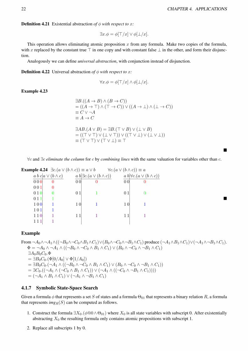
∀c and ∃c eliminate the column for c by combining lines with the same valuation for variables other than c.

Example 4.24 ∃c.(a ∨ (b ∧ c)) ≡ a ∨ b ∀c.(a ∨ (b ∧ c)) ≡ aa b c a ∨ (b ∧ c)0 0 0 00 0 1 00 1 0 00 1 1 11 0 0 11 0 1 11 1 0 11 1 1 1

a b ∃c.(a ∨ (b ∧ c))0 0 0

0 1 1

1 0 1

1 1 1

a b ∀c.(a ∨ (b ∧ c))0 0 0

0 1 0

1 0 1

1 1 1

�

Example

From ¬A0∧¬A1∧((¬B0∧¬C0∧B1∧C1)∨(B0∧¬C0∧¬B1∧C1) produce (¬A1∧B1∧C1)∨(¬A1∧¬B1∧C1).Φ = ¬A0 ∧ ¬A1 ∧ ((¬B0 ∧ ¬C0 ∧B1 ∧ C1) ∨ (B0 ∧ ¬C0 ∧ ¬B1 ∧ C1)∃A0B0C0.Φ= ∃B0C0.(Φ[0/A0] ∨ Φ[1/A0])= ∃B0C0.(¬A1 ∧ ((¬B0 ∧ ¬C0 ∧B1 ∧ C1) ∨ (B0 ∧ ¬C0 ∧ ¬B1 ∧ C1))= ∃C0.((¬A1 ∧ (¬C0 ∧B1 ∧ C1)) ∨ (¬A1 ∧ ((¬C0 ∧ ¬B1 ∧ C1))))= (¬A1 ∧B1 ∧ C1) ∨ (¬A1 ∧ ¬B1 ∧ C1)

4.1.7 Symbolic State-Space Search

Given a formula φ that represents a set S of states and a formula Θ01 that represents a binary relationR, a formulathat represents imgR(S) can be computed as follows.

1. Construct the formula ∃X0.(φ@0∧Θ01) where X0 is all state variables with subscript 0. After existentiallyabstracting X0 the resulting formula only contains atomic propositions with subscript 1.

2. Replace all subscripts 1 by 0.

4.1. STATE-SPACE SEARCH 23

We denote the resulting formula by imgΘ01(φ).This image operation can be applied repeatedly to compute formulas that represent the states reached with arbi-

trarily long sequences of actions. This leads to a symbolic breadth-first search algorithm for computing reachablestates.

Algorithm 4.25 (Breadth-first search with formulas) The algorithm takes as its first input a formula I thatrepresents one or more initial states. This formula is over the set X of state variables. We denote the formula Iwith all atomic propositions with subscript 0 as I@0.

The second input to the algorithm is a formula Θ01 which represents a binary relation over the set of states. Itis over atomic propositions which are the state variables with subscripts 0 and 1.

1. i := 0

2. Φ0 := I@0

3. i := i+ 1

4. Φi := Φi−1 ∨ imgΘ01(Φi−1)

5. if Φi 6|= Φi−1 then go to step 3

After the computation has terminated, the formula Φi represents the set of all reachable states.

References

For the solution of reachability problems in discrete transition systems the use of propositional logic as a repre-sentation of sets and relations was first proposed in the works by Coudert et al. [CBM90, CM90] and Burch et al.[BCL+94].

The use of these logic-based techniques was possible with (ordered, reduced) Binary Decision Diagrams[Bry92], generally known as BDDs or OBDDs. BDDs are a restrictive normal form that guarantees a canonic-ity property: any two logically equivalent Boolean formulas are represented by a unique BDD. The canonicityproperty guarantees the polynomial-time solvability of many central problems about Boolean formulas, includingequivalence, satisfiability, and model-counting. Though in some cases necessarily (even exponentially) larger thanunlimited Boolean formulas, BDDs also in practice often lead to compact enough representations when unlimitedformulas would in practice be too large.

Other similar normal forms, with useful polynomial-time operations, exist, including Decomposable NegationNormal form (DNNF) [Dar01, Dar02]. There are interesting connections between this type of normal forms andthe Davis-Putnam procedure [HD05].

Problems with scalability of BDD-based methods was well-understood already in mid-1990ies. Another wayof using the propositional logic for solving state-space search problems was proposed by Kautz and Selman[KS92] in 1992, and in 1996 they demonstrated it to be often far better scalable than alternative search methodsfor solving state-space search problems in AI [KS96]. This method was based on mapping one reachability query,whether a state satisfying a given goal formula is reachable in a given number of steps from a specified initialstate. The method suffered from the large size of the formulas far less than BDDs, and was soon shown to be inmany cases far better scalable than BDD-based methods for example in Computer Aided Verification, for solvingthe model-checking problem [BCCZ99].

In Section 4.1.5 we only presented the most basic translation of action sequences to propositional formulas,with the exactly one action at each step. This is what is known as a sequential encoding. This representationsuffers from the possibility of sequences of actions a1, . . . , an that are independent of each other, and whichtherefore can be permuted to every one of n! different orders. So called parallel encodings allow several actionsor events at the same time [KS96, RHN06]. Having several actions can simultaneous decreases the horizon length.This substantially improves the scalability of SAT-based methods in the main applications including the planning,diagnosis, and model-checking problems.

Index

BDD, 23binary decision diagrams, 23Boolean Constraint Propagation, 12clause, 6CNF, 6combinatorial explosion, 14complement (of a literal), 11conjunctive normal form, 6consistency, 6Davis-Putnam procedure, 12Davis-Putnam-Logemann-Loveland procedure, 12disjunctive normal form, 7DNF, 7effect, 18empty clause, 11existential abstraction, 21image operation, 20, 23inconsistency, 6literal, 6negation normal form, 7NNF, 7OBDD, 23precondition, 18resolution, 11satisfiability, 6Shannon expansion, 21term, 6unit clause, 11unit propagation, 12unit resolution, 11unit subsumption, 12universal abstraction, 22valuation, 3weakest preconditions, 19

24

Bibliography

[AS09] Gilles Audemard and Laurent Simon. Predicting learnt clauses quality in modern SAT solvers. InProceedings of the 21st International Joint Conference on Artificial Intelligence, pages 399–404.Morgan Kaufmann Publishers, 2009.

[BCCZ99] Armin Biere, Alessandro Cimatti, Edmund M. Clarke, and Yunshan Zhu. Symbolic model checkingwithout BDDs. In W. R. Cleaveland, editor, Tools and Algorithms for the Construction and Analysisof Systems, Proceedings of 5th International Conference, TACAS’99, volume 1579 of Lecture Notesin Computer Science, pages 193–207. Springer-Verlag, 1999.

[BCL+94] Jerry R. Burch, Edmund M. Clarke, David E. Long, Kenneth L. MacMillan, and David L. Dill.Symbolic model checking for sequential circuit verification. IEEE Transactions on Computer-AidedDesign of Integrated Circuits and Systems, 13(4):401–424, 1994.

[Bry92] R. E. Bryant. Symbolic Boolean manipulation with ordered binary decision diagrams. ACM Com-puting Surveys, 24(3):293–318, September 1992.

[Byl94] Tom Bylander. The computational complexity of propositional STRIPS planning. Artificial Intelli-gence, 69(1-2):165–204, 1994.

[CBM90] Olivier Coudert, Christian Berthet, and Jean Christophe Madre. Verification of synchronous sequen-tial machines based on symbolic execution. In Joseph Sifakis, editor, Automatic Verification Methodsfor Finite State Systems, International Workshop, Grenoble, France, June 12-14, 1989, Proceedings,volume 407 of Lecture Notes in Computer Science, pages 365–373. Springer-Verlag, 1990.

[CM90] Olivier Coudert and Jean Christophe Madre. A unified framework for the formal verification ofsequential circuits. In Computer-Aided Design, 1990. ICCAD-90. Digest of Technical Papers., 1990IEEE International Conference on, pages 126–129. IEEE Computer Society Press, 1990.

[CMV09] Benjamin Chambers, Panagiotis Manolios, and Daron Vroon. Faster SAT solving with better CNFgeneration. In Proceedings of the Conference on Design, Automation and Test in Europe, pages1590–1595, 2009.

[Coo71] Stephen A. Cook. The complexity of theorem-proving procedures. In Proceedings of the ThirdAnnual ACM Symposium on Theory of Computing, pages 151–158, 1971.

[Dar01] Adnan Darwiche. Decomposable negation normal form. Journal of the ACM, 48(4):608–647, 2001.

[Dar02] Adnan Darwiche. A compiler for deterministic, decomposable negation normal form. In Proceedingsof the 18th National Conference on Artificial Intelligence (AAAI-2002) and the 14th Conference onInnovative Applications of Artificial Intelligence (IAAI-2002), pages 627–634, 2002.

[DG84] William F. Dowling and Jean H. Gallier. Linear-time algorithms for testing the satisfiability of propo-sitional Horn formulae. Journal of Logic Programming, 1(3):267–284, 1984.

[Dij75] Edsger W. Dijkstra. Guarded commands, nondeterminacy and formal derivation of programs. Com-munications of the ACM, 18(8):453–457, 1975.

[DLL62] M. Davis, G. Logemann, and D. Loveland. A machine program for theorem proving. Communica-tions of the ACM, 5:394–397, 1962.

25

26 BIBLIOGRAPHY

[DP60] M. Davis and H. Putnam. A computing procedure for quantification theory. Journal of the ACM,7(3):201–215, 1960.

[GJ79] M. R. Garey and D. S. Johnson. Computers and Intractability. W. H. Freeman and Company, SanFrancisco, 1979.

[GW83] Hana Galperin and Avi Wigderson. Succinct representations of graphs. Information and Control,56:183–198, 1983. See [Loz88] for a correction.

[HD05] Jinbo Huang and Adnan Darwiche. DPLL with a trace: From SAT to knowledge compilation. InLeslie Pack Kaelbling, editor, Proceedings of the 19th International Joint Conference on ArtificialIntelligence, pages 156–162. Professional Book Center, 2005.

[KS92] Henry Kautz and Bart Selman. Planning as satisfiability. In Bernd Neumann, editor, Proceedings ofthe 10th European Conference on Artificial Intelligence, pages 359–363. John Wiley & Sons, 1992.

[KS96] Henry Kautz and Bart Selman. Pushing the envelope: planning, propositional logic, and stochas-tic search. In Proceedings of the 13th National Conference on Artificial Intelligence and the 8thInnovative Applications of Artificial Intelligence Conference, pages 1194–1201. AAAI Press, 1996.

[LB90] Antonio Lozano and Jose L. Balcazar. The complexity of graph problems for succinctly representedgraphs. In Manfred Nagl, editor, Graph-Theoretic Concepts in Computer Science, 15th InternationalWorkshop, WG’89, number 411 in Lecture Notes in Computer Science, pages 277–286. Springer-Verlag, 1990.

[Loz88] Antonio Lozano. NP-hardness of succinct representations of graphs. Bulletin of the European Asso-ciation for Theoretical Computer Science, 35:158–163, June 1988.

[MMZ+01] Matthew W. Moskewicz, Conor F. Madigan, Ying Zhao, Lintao Zhang, and Sharad Malik. Chaff:engineering an efficient SAT solver. In Proceedings of the 38th ACM/IEEE Design AutomationConference (DAC’01), pages 530–535. ACM Press, 2001.

[MSS96] Joao P. Marques-Silva and Karem A. Sakallah. GRASP: A new search algorithm for satisfiability.In Computer-Aided Design, 1996. ICCAD-96. Digest of Technical Papers., 1996 IEEE/ACM Inter-national Conference on, pages 220–227, 1996.

[PD07] Knot Pipatsrisawat and Adnan Darwiche. A lightweight component caching scheme for satisfiabilitysolvers. In Joao Marques-Silva and Karem A. Sakallah, editors, Proceedings of the 8th InternationalConference on Theory and Applications of Satisfiability Testing (SAT-2007), volume 4501 of LectureNotes in Computer Science, pages 294–299. Springer-Verlag, 2007.

[RHN06] Jussi Rintanen, Keijo Heljanko, and Ilkka Niemela. Planning as satisfiability: parallel plans andalgorithms for plan search. Artificial Intelligence, 170(12-13):1031–1080, 2006.

[SLM92] B. Selman, H. Levesque, and D. Mitchell. A new method for solving hard satisfiability problems. InProceedings of the 11th National Conference on Artificial Intelligence, pages 46–51, 1992.

[Tse68] G. S. Tseitin. On the complexity of derivations in propositional calculus. In A. O. Slisenko, editor,Studies in Constructive Mathematics and Mathematical Logic, Part II, pages 115–125. ConsultantsBureau, 1968.