PROPOSED SYNTHETIC AND GROUP RUNS CONTROL …

PROPOSED SYNTHETIC AND GROUP RUNS

CONTROL CHARTS BASED ON RUNS RULES X AND DOUBLE SAMPLING np METHODS

CHONG ZHI LIN

UNIVERSITI SAINS MALAYSIA

2015

PROPOSED SYNTHETIC AND GROUP RUNS CONTROL CHARTS BASED ON RUNS RULES X

AND DOUBLE SAMPLING np METHODS

by

CHONG ZHI LIN

Thesis submitted in fulfillment of the requirements for the degree of

Doctor of Philosophy

August 2015

ii

ACKNOWLEDGEMENTS

I would like to express my sincere gratitude to several individuals and

organizations for supporting me throughout my Ph.D. study. First and foremost, I

wish to express my sincere thanks to my supervisor, Professor Michael Khoo Boon

Chong, for his patience, enthusiasm, insightful comments, invaluable suggestions,

helpful information, practical advice and unceasing ideas which have helped me

tremendously at all times in my research and writing of this thesis. His immense

knowledge, profound experience and professional expertise in Statistical Quality

Control (SQC) has enabled me to complete this research successfully. I am thankful

to him for his precious time in guiding me, answering my queries, correcting and

improving the English in my thesis. Without his guidance and relentless help, this

thesis would not have been possible. I could not have imagined having a better

supervisor in my study.

I also wish to express my sincere thanks to Universiti Sains Malaysia (USM)

for accepting me into the Ph.D. program. In addition, I am deeply indebted to the

Ministry of Higher Education, Malaysia for granting me the MyPhD scholarship.

This financial support has enabled me to complete my Ph.D. study successfully. Also,

I thank the School of Mathematical Sciences (PPSM), USM for sponsoring me to

conferences.

My sincere thanks goes to Professor Ahmad Izani Md. Ismail, Dean of PPSM,

USM, for his continuous support and assistance in my postgraduate study. I am also

grateful to the lecturers and staff of PPSM for their kindness, hospitality and

technical support. In addition, I would like to acknowledge the Institute of

iii

Postgraduate Studies, USM and PPSM for organizing various workshops, which

have helped me in improving my research and programming skills.

I also wish to express my deepest thanks to my parents and two elder brothers.

Their unwavering support and encouragement is my source of strength. I am also

thankful to my beloved fiancée, Low Zeng Yee. She is always there caring for me,

cheering me up and stood by me through the peaks and valleys of my life.

Additionally, I owe my gratitude to all my friends, church members and pastors for

giving me their company, friendship, moral support and advice. Last but not least, I

am grateful to Jesus and the Almighty God for the abundant blessings and unfailing

love for me.

iv

TABLE OF CONTENTS

Page

Acknowledgements ii

Table of Contents iv

List of Tables x

List of Figures xiv

List of Notations xv

List of Publications xxv

Abstrak xxvi

Abstract xxviii

CHAPTER 1 – INTRODUCTION

1.1 Statistical Process Control (SPC) 1

1.2 Problem Statement 4

1.3 Objectives of the Thesis 6

1.4 Organization of the Thesis 6

CHAPTER 2 – LITERATURE REVIEW

2.1 Introduction 9

2.2 Runs Rules Type Control Charts 9

2.2.1 Standard m-of-k ( /m k ) Runs Rules Control Chart 13

2.2.2 Improved m-of-k ( /I m k− ) Runs Rules Control Chart 14

2.2.3 Revised m-of-k ( /−R m k ) Runs Rules Control Chart 15

2.3 np Type Control Charts 20

v

2.3.1 Single Sampling (SS) np Control Chart 22

2.3.2 Double Sampling (DS) np Control Chart 24

2.4 Related Control Charts for Variables Data 28

2.4.1 Synthetic X Control Chart 28

2.4.2 Group Runs (GR) X Control Chart 31

2.4.3 EWMA X Control Chart 34

2.5 Related Control Charts for Attribute Data 36

2.5.1 Synthetic np Control Chart 36

2.5.2 Group Runs (GR) np Control Chart 38

2.5.3 Variable Sample Size (VSS) np Control Chart 40

2.5.4 EWMA np Control Chart 41

2.5.5 CUSUM np and CUSUM(FIR) np Control Charts 42

2.6 ARL as a Performance Measure of a Chart 43

CHAPTER 3 – PROPOSED SYNTHETIC /−R m k AND GR /R m k− RUNS RULES CHARTS

3.1 Introduction 44

3.2 Synthetic /−R m k Runs Rule Chart 45

3.2.1 Charting Statistics and Performance Measure of the Synthetic /−R m k Runs Rule Chart

45

3.2.2 Optimal Design of the Synthetic /−R m k Runs Rule Chart

47

3.2.3 An Illustrative Example 49

3.3 GR /−R m k Runs Rule Chart 53

3.3.1 Charting Statistics and Performance Measure of the GR /−R m k Runs Rule Chart

53

3.3.2 Optimal Design of the GR /−R m k Runs Rule Chart 55

vi


CHAPTER 4 – PROPOSED SYNTHETIC DS np AND GR DS np CHARTS

4.1 Introduction 62

4.2 Synthetic DS np Chart 62

4.2.1 Charting Statistics and Performance Measure of the Synthetic DS np Chart

62

4.2.2 Optimal Design of the Synthetic DS np Chart 64


4.3 GR DS np Chart 69

4.3.1 Charting Statistics and Performance Measure of the GR DS np Chart

69

4.3.2 Optimal Design of the GR DS np Chart 70


CHAPTER 5 – A PERFORMANCE COMPARISON OF THE PROPOSED CHARTS WITH EXISTING CHARTS

5.1 Introduction 75

5.2 A Performance Comparison of the Synthetic /−R m k and GR /−R m k Charts with Existing Charts

75

5.3 A Performance Comparison of the Synthetic DS np and GR DS np Charts with Existing Charts

83

CHAPTER 6 – CONCLUSIONS AND FUTURE RESEARCH

6.1 Introduction 98

6.2 Contributions and Findings of the Research 98

6.3 Suggestions for Future Research 101

vii

REFERENCES 104

APPENDIX A – OPTIMIZATION PROGRAMS FOR OTHER CHARTS UNDER COMPARISON

A.1 An Optimization Program for the /−R m k Runs Rule Chart 116

A.2 An Optimization Program for the SS np Chart 119

A.3 An Optimization Program for the DS np Chart 121

A.4 An Optimization Program for the synthetic X Chart 124

A.5 An Optimization Program for the GR X Chart 127

A.6 An Optimization Program for the EWMA X Chart 129

A.7 An Optimization Program for the Synthetic np Chart 134

A.8 An Optimization Program for the GR np Chart 136

A.9 An Optimization Program for the VSS np Chart 137

A.10 An Optimization Program for the EWMA np Chart 141

A.11 An Optimization Program for the CUSUM np and CUSUM (FIR) np Charts

143

APPENDIX B – MARKOV CHAIN METHOD TO COMPUTE THE ARLS OF CONTROL CHARTS

B.1 Markov Chain Model to Obtain the tpm of 4 / 5R − Runs Rule Chart

145

B.2 Markov Chain Model to Obtain the EWMA X Chart’s ARL 149

B.3 Markov Chain Model to Obtain the VSS np Chart’s ARL 150

B.4 Markov Chain Model to Obtain the EWMA np Chart’s ARL 152

B.5 Markov Chain Model to Obtain the CUSUM np Chart’s ARL 154

viii

APPENDIX C – OPTIMIZATION PROGRAMS FOR THE SYNTHETIC /−R m k AND GR /−R m k RUNS RULES CHARTS

C.1 An Optimization Program for the Synthetic /−R m k Runs Rule Chart

157

C.2 An Optimization Program for the GR /−R m k Runs Rule Chart 161

APPENDIX D – OPTIMIZATION PROGRAMS FOR THE SYNTHETIC DS np AND GR DS np CHARTS

D.1 An Optimization Program for the Synthetic DS np Chart 166

D.2 An Optimization Program for the GR DS np Chart 170

APPENDIX E – MONTE CARLO SIMULATION PROGRAMS

E.1 Monte Carlo Simulation Programs for the Synthetic /−R m k Runs Rule Chart

176

E.1.1 Synthetic 2 / 3R − Runs Rule Chart 176

E.1.2 Synthetic 4 / 5R − Runs Rule Chart 178

E.2 Monte Carlo Simulation Programs for the GR /−R m k Runs Rule Chart

181

E.2.1 GR 2 / 3R − Runs Rule Chart 181

E.2.2 GR 4 / 5R − Runs Rule Chart 183

E.3 Monte Carlo Simulation Program for the Synthetic DS np Chart 186

E.4 Monte Carlo Simulation Program for the GR DS np Chart 187

E.5 A Simulation Program for the Illustrative Example 188

APPENDIX F – A PERFORMANCE COMPARISON OF THE SYNTHETIC /R m k− AND GR /R m k− CHARTS WITH EXISTING CHARTS

F.1 Additional Results for a performance comparison of the Synthetic /−R m k and GR /−R m k Charts with Existing Charts

192

ix

APPENDIX G – A PERFORMANCE COMPARISON OF THE SYNTHETIC DS np AND GR DS np CHARTS WITH EXISTING CHARTS

G.1 Additional Results for a performance comparison of the Synthetic DS np and GR DS np Charts with Existing Charts

201

x

LIST OF TABLES

Page

Table 2.1 The tpm, R1, for the 2 / 3−R runs rule

19

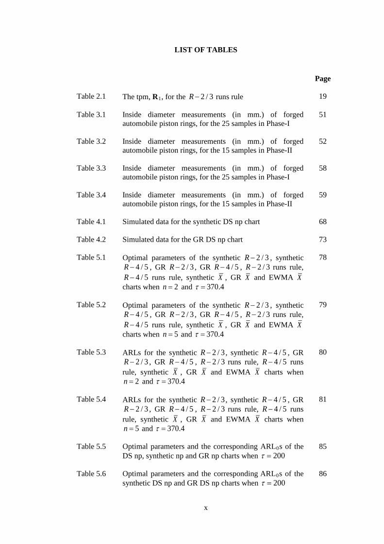
Table 3.1 Inside diameter measurements (in mm.) of forged automobile piston rings, for the 25 samples in Phase-I

51

Table 3.2 Inside diameter measurements (in mm.) of forged automobile piston rings, for the 15 samples in Phase-II

52

Table 3.3 Inside diameter measurements (in mm.) of forged automobile piston rings, for the 25 samples in Phase-I

58

Table 3.4 Inside diameter measurements (in mm.) of forged automobile piston rings, for the 15 samples in Phase-II

59

Table 4.1 Simulated data for the synthetic DS np chart

68

Table 4.2 Simulated data for the GR DS np chart

73

Table 5.1 Optimal parameters of the synthetic 2 / 3R − , synthetic 4 / 5R − , GR 2 / 3R − , GR 4 / 5R − , 2 / 3R − runs rule, 4 / 5R − runs rule, synthetic X , GR X and EWMA X

charts when 2n = and 370.4τ =

78

Table 5.2 Optimal parameters of the synthetic 2 / 3R − , synthetic 4 / 5R − , GR 2 / 3R − , GR 4 / 5R − , 2 / 3R − runs rule, 4 / 5R − runs rule, synthetic X , GR X and EWMA X

charts when 5=n and 370.4τ =

79

Table 5.3 ARLs for the synthetic 2 / 3R − , synthetic 4 / 5R − , GR 2 / 3R − , GR 4 / 5R − , 2 / 3R − runs rule, 4 / 5R − runs

rule, synthetic X , GR X and EWMA X charts when 2n = and 370.4τ =

80

Table 5.4 ARLs for the synthetic 2 / 3R − , synthetic 4 / 5R − , GR 2 / 3R − , GR 4 / 5R − , 2 / 3R − runs rule, 4 / 5R − runs

rule, synthetic X , GR X and EWMA X charts when 5=n and 370.4τ =

81

Table 5.5 Optimal parameters and the corresponding ARL0s of the DS np, synthetic np and GR np charts when 200τ =

85

Table 5.6 Optimal parameters and the corresponding ARL0s of the synthetic DS np and GR DS np charts when 200τ =

86

xi

Table 5.7 Optimal parameters and the corresponding ARL0s of the DS np, synthetic np and GR np charts when 370.4τ =

87

Table 5.8 Optimal parameters and the corresponding ARL0s of the synthetic DS np and GR DS np charts when 370.4τ =

88

Table 5.9 ARL1s of the DS np, synthetic np, GR np, synthetic DS np and GR DS np charts when 200τ =

90

Table 5.10 ARL1s of the DS np, synthetic np, GR np, synthetic DS np and GR DS np charts when 370.4τ =

91

Table 5.11 ARL1 comparison of the optimal charts, based on 200τ = , optγ = 1.5, 0p = 0.005 and n = {100, 200}

94

Table 5.12 ARL1 comparison of the optimal charts, based on 200τ = , optγ = 1.5, 0p = 0.005 and n = {400, 800}

95

Table 5.13 ARL1 comparison of the optimal charts, based on 370.4τ = , optγ = 1.5, 0p = 0.005 and n = {100, 200}

96

Table 5.14 ARL1 comparison of the optimal charts, based on 370.4τ = , optγ = 1.5, 0p = 0.005 and n = {400, 800}

97

Table B.1 Steps to decompose the composite pattern, D2, for the 4 / 5R − runs rule chart

147

Table B.2 The tpm, R1, for the 4 / 5R − runs rule chart

148

Table F.1 Optimal parameters of the synthetic 2 / 3R − , synthetic 4 / 5R − , GR 2 / 3R − , GR 4 / 5R − , 2 / 3R − runs rule, 4 / 5R − runs rule, synthetic X , GR X and EWMA X

charts when 10n = and 370.4τ =

193


charts when 2n = and 500τ =

194



195

xii



196

Table F.5 ARLs for the synthetic 2 / 3R − , synthetic 4 / 5R − , GR 2 / 3R − , GR 4 / 5R − , 2 / 3R − runs rule, 4 / 5R − runs

rule, synthetic X , GR X and EWMA X charts when 10n = and 370.4τ =

197


rule, synthetic X , GR X and EWMA X charts when 2n = and 500τ =

198


rule, synthetic X , GR X and EWMA X charts when 5=n and 500τ =

199


rule, synthetic X , GR X and EWMA X charts when 10n = and 500τ =

200

Table G.1 ARL1 comparison of the optimal charts, based on 200τ = , optγ = 2.0, 0p = 0.01 and n = {50, 100}

202


203

Table G.3 ARL1 comparison of the optimal charts, based on 370.4τ = , optγ = 2.0, 0p = 0.01 and n = {50, 100}

204


205


206


207


208

xiii


209

xiv

LIST OF FIGURES

Page

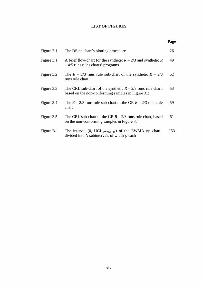
Figure 2.1 The DS np chart’s plotting procedure

26

Figure 3.1 A brief flow-chart for the synthetic R – 2/3 and synthetic R – 4/5 runs rules charts’ programs

49

Figure 3.2 The R – 2/3 runs rule sub-chart of the synthetic R – 2/3 runs rule chart

52

Figure 3.3 The CRL sub-chart of the synthetic R – 2/3 runs rule chart, based on the non-conforming samples in Figure 3.2

53

Figure 3.4 The R – 2/3 runs rule sub-chart of the GR R – 2/3 runs rule chart

59

Figure 3.5 The CRL sub-chart of the GR R – 2/3 runs rule chart, based on the non-conforming samples in Figure 3.4

61

Figure B.1 The interval (0, UCLEWMA np) of the EWMA np chart, divided into N subintervals of width ψ each

153

xv

LIST OF NOTATIONS

Notations and abbreviations used in this thesis are listed as follows: SPC Statistical Process Control

SQC Statistical Quality Control

SAS Statistical Analysis System

SS Single sampling

DS Double sampling

GR Group runs

MGR Modified GR

UGR Unit and GR

SSGR Side sensitive GR

SSMGR Side sensitive modified GR

CRL Conforming run length

VSS Variable sample size

VSI Variable sampling interval

EWMA Exponentially weighted moving average

CUSUM Cumulative sum

SPRT Sequential probability ratio test

Syn-np Synthetic np and np charts

/m k m-of-k

/I m k− Improved m-of-k

/−R m k Revised m-of-k

ARL Average run length

0ARL In-control ARL

1ARL Out-of-control ARL

xvi

1, minARL Minimum value of 1ARL

MRL Median run length

ASS Average sample size

0ASS In-control ASS

ATS Average time to signal

ANOS Average number of observations to signal

AEQL Average extra quadratic loss

EARL Expected value of the ARL

FIR Fast initial response

0µ In-control mean

1µ Out-of-control mean

0σ In-control standard deviation

ˆ Xσ Sample standard deviation estimated from Phase-I samples

δ Size of the standardized mean shift

γ Ratio of 1p over 0p

optγ Desired γ value where a quick detection is required

⌊ ⋅ ⌋ Largest integer less than or equal to its argument

⌈ ⋅ ⌉ Smallest integer larger than or equal to its argument

d Control limit constant

1d Inner control limit constant

2d Outer control limit constant

0e Number of non-conforming units in a sample

1e Number of non-conforming units in the first sample

2e Number of non-conforming units in the second sample

xvii

ue Number of non-conforming items in sample u

n Sample size

p Fraction of non-conforming units

0p In-control p

1p Out-of-control p

T Run length variable

X Grand sample mean estimated from Phase-I samples

CL Center line

WL Warning limit

LCL Lower control limit

UCL Upper control limit

iid Independent and identically distributed

cdf Cumulative distribution function

( ).Φ Standard normal cdf

tpm Transition probability matrix

I Identity matrix

1 A vector with all of its elements equal to unity

0 A vector with all of its elements equal to zero

1R Transition probability matrix for the transient states

S Initial probability vector

1S Initial probability vector, where the first entry is unity and zeros in all other entries

τ A desired in-control ARL value

xviii

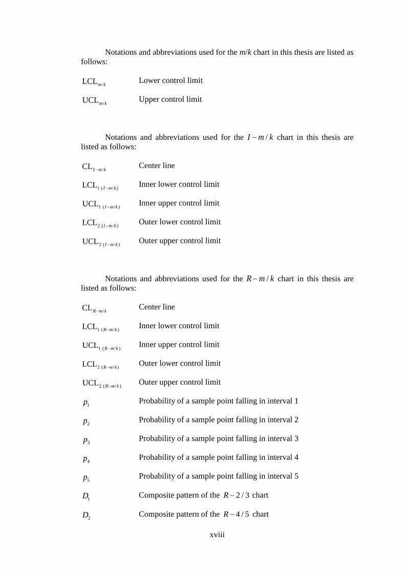
Notations and abbreviations used for the m/k chart in this thesis are listed as follows:

/LCLm k Lower control limit

/UCLm k Upper control limit

Notations and abbreviations used for the /I m k− chart in this thesis are listed as follows:

/CLI m k− Center line

1 ( / )LCL I m k− Inner lower control limit

1 ( / )UCL I m k− Inner upper control limit

2 ( / )LCL I m k− Outer lower control limit

2 ( / )UCL I m k− Outer upper control limit

Notations and abbreviations used for the /R m k− chart in this thesis are listed as follows:

/CLR m k− Center line

1 ( / )LCL R m k− Inner lower control limit

1 ( / )UCL R m k− Inner upper control limit

2 ( / )LCL R m k− Outer lower control limit

2 ( / )UCL R m k− Outer upper control limit

1p Probability of a sample point falling in interval 1





1D Composite pattern of the 2 / 3R − chart

2D Composite pattern of the 4 / 5R − chart

xix

Notations and abbreviations used for the synthetic X chart in this thesis are listed as follows:

Syn LCL X LCL of the X sub-chart

Syn UCL X UCL of the X sub-chart

Syn CRL X CRL for the CRL sub-chart

Syn XL LCL of the CRL sub-chart

Notations and abbreviations used for the GR X chart in this thesis are listed as follows:

(GR )CRLi X thi CRL value

GR XL LCL of the extended CRL sub-chart

Notations and abbreviations used for the EWMA X chart in this thesis are listed as follows: λ Smoothing constant

α Width constant of each subinterval

uZ Plotting statistics of the chart at sample u

EWMA XK Width constant

EWMA Xk A multiplier controlling the width of the chart’s control limits

2R Transition probability matrix with the absorbing state

Q Transition probability matrix for the transient states

,i jQ Transition probability for entry (i, j) in matrix Q

Notations and abbreviations used for the synthetic /R m k− chart in this thesis are listed as follows:

Syn /CL R m k− Center line

xx

1 (Syn / )LCL R m k− Inner lower control limit

1 (Syn / )UCL R m k− Inner upper control limit

2 (Syn / )LCL R m k− Outer lower control limit

2 (Syn / )UCL R m k− Outer upper control limit

(Syn / )CRL −i R m k thi CRL for the CRL sub-chart

Syn /R m kL − LCL of the CRL sub-chart

iY Number of samples taken (including the ending non-conforming sample) until the ith non-conforming sample is signalled by the

/−R m k runs rule sub-chart

Notations and abbreviations used for the GR /R m k− chart in this thesis are listed as follows:

GR /CL R m k− Center line

1 (GR 2/3)LCL R− Inner lower control limit

1 (GR 2/3)UCL R− Inner upper control limit

2 (GR 2/3)LCL R− Outer lower control limit

2 (GR 2/3)UCL R− Outer upper control limit

(GR / )CRLi R m k− thi CRL for the extended CRL sub-chart

GR R m kL /− LCL of the extended CRL sub-chart

iY Number of samples taken (including the ending non-conforming sample) until the ith non-conforming sample is signalled by the

/−R m k runs rule sub-chart

Abbreviation used for the SS np chart in this thesis is listed as follows:

SS npUCL Upper control limit

xxi

Notations and abbreviations used for the DS np chart in this thesis are listed as follows:

1n First sample size

2n Second sample size

1Ac First sample acceptance number

1Re First sample rejection number

2Ac Second sample acceptance number

DS npWL Warning limit

DS npLCL Lower control limit

1 (DS np)UCL UCL of the first sampling stage

2 (DS np)UCL UCL of the second sampling stage

Notations and abbreviations used for the synthetic np chart in this thesis are listed as follows: c Acceptance number

Syn npUCL UCL of the np sub-chart

Syn npCRL CRL for the CRL sub-chart

Syn npL LCL of the CRL sub-chart

Notations and abbreviations used for the GR np chart in this thesis are listed as follows:

GR npUCL UCL of the np sub-chart

(GR np)CRLi thi CRL for the extended CRL sub-chart

GR npL LCL of the extended CRL sub-chart

xxii

Notations and abbreviations used for the VSS np chart in this thesis are listed as follows:

1n Small sample size

2n Large sample size

1 (VSS np)WL WL when the sample size is small

2 (VSS np)WL WL when the sample size is large

1 (VSS np)UCL UCL when the sample size is small

2 (VSS np)UCL UCL when the sample size is large

1e Number of non-conforming units in a sample of size 1n

2e Number of non-conforming units in a sample of size 2n

β False alarm risk

P In-control transition probability matrix

q Out-of control transition probability matrix

Notations and abbreviations used for the EWMA np chart in this thesis are listed as follows: λ Smoothing constant

ψ Width constant of each subinterval

uZ Plotting statistics of the chart at sample u

EWMA npLCL Lower control limit

EWMA npUCL Upper control limit

P Transition probability matrix for the transient states

,i jP Transition probability for entry (i, j) in matrix P

xxiii

Notations and abbreviations used for the CUSUM np chart in this thesis are listed as follows:

uS + Plotting statistics

k Pre-specified non-negative value

CUSUM npUCL Upper control limit

*1p Out-of-control nonconforming rate where a quick detection is

important

T Transition probability matrix for the transient states

,i jT Transition probability for entry (i, j) in matrix T

4R Transition probability matrix with the absorbing states

Notations and abbreviations used for the synthetic DS np chart in this thesis are listed as follows:



Syn DSWL Warning limit

1 (Syn DS)UCL UCL of the first sampling stage

2 (Syn DS)UCL UCL of the second sampling stage

(Syn DS)CRLi thi CRL for the CRL sub-chart

Syn DSL LCL of the CRL sub-chart

Notations and abbreviations used for the GR DS np chart in this thesis are listed as follows:



GR DSWL Warning limit

1 (GR DS)UCL UCL of the first sampling stage

xxiv

2 (GR DS)UCL UCL of the second sampling stage

(GR DS)CRLi thi CRL for the extended CRL sub-chart

GR DSL LCL of the extended CRL sub-chart

xxv

LIST OF PUBLICATIONS

Journals

1. Chong, Z.L., Khoo, M.B.C. and Castagliola, P. (2014). Synthetic double sampling np control chart for attributes. Computers & Industrial Engineering, 75(1), 157-169. [ISSN: 0360-8352][2013 impact factor: 1.690]

2. Chong, Z.L., Khoo, M.B.C., Lee, M.H. and Chen, C.-H. (2015). Group runs

revised m-of-k runs rule control chart. Communications in Statistics - Theory and Methods. Under revision. [Print ISSN: 0361-0926; Online ISSN: 1532-415X][2013 impact factor: 0.284]

3. Chong, Z.L., Khoo, M.B.C., Teoh, W.L. and Yeong, W.C. (2015). A Group runs double sampling np control chart for attributes. Sains Malaysiana. Under review. [ISSN: 0126-6039][2013 impact factor: 0.480]

Proceedings

1. Chong, Z.L., Khoo, M.B.C., Teoh, W.L. and Teh, S.Y. (2015). A synthetic

revised m-of-k runs rule control chart. Proceedings of the 2015 7th International Conference on Research and Education in Mathematics, ICREM7 2015, Renaissance Kuala Lumpur Hotel, Kuala Lumpur, Malaysia. Accepted. [MJMS, Print ISSN: 1823-8343; Online ISSN: 2289-750X]

xxvi

CADANGAN CARTA-CARTA KAWALAN SINTETIK DAN LARIAN KUMPULAN BERDASARKAN KAEDAH-KAEDAH X PETUA LARIAN

DAN np PENSAMPELAN GANDA DUA

ABSTRAK

Carta kawalan adalah alat yang penting untuk memantau satu atau lebih cirian

kualiti yang diminati dalam proses pengeluaran. Carta kawalan X Shewhart yang

klasik adalah carta kawalan pembolehubah yang paling luas digunakan dalam

industri pembuatan dan perkhidmatan untuk memantau min sesuatu proses dengan

data selanjar kerana kesenangannya kepada pekerja-pekerja industri. Carta kawalan

X Shewhart adalah sangat berkesan untuk mengesan anjakan besar dalam min

proses. Walau bagaimanapun, carta X Shewhart adalah kurang peka terhadap

anjakan min yang kecil dan sederhana. Ini merupakan kelemahan utama carta X

Shewhart. Petua-petua larian biasanya digunakan untuk meningkatkan kepekaan

carta X Shewhart yang klasik bagi pengesanan anjakan min proses yang kecil dan

sederhana. Suatu petua larian yang lebih baru dan berkesan ialah skema petua larian

m-daripada-k yang disemak semula ( /−R m k ) untuk data selanjar. Sebaliknya,

dalam pemantauan proses yang melibatkan data atribut, carta kawalan np

pensampelan ganda dua (DS) adalah carta yang berkesan untuk mengesan

anjakan kecil hingga sederhana dalam ketidakpatuhan pecahan barangan

daripada sesuatu proses. Didorong oleh keperluan untuk meningkatkan

prestasi carta yang sedia ada, kami menggabungkan prosedur carta sintetik

dan larian kumpulan (GR) dengan skema petua larian /−R m k dan carta np DS.

Objektif utama tesis ini adalah untuk mencadangkan empat reka bentuk optimum

carta-carta kawalan yang baru dengan meminimumkan panjang larian purata luar

xxvii

kawalan ( 1ARL ) bagi (i) carta X petua larian /−R m k sintetik, (ii) carta X petua

larian /−R m k GR, (iii) carta np DS sintetik, dan (iv) carta np DS GR. Keputusan

1ARL carta-carta optimum menunjukkan bahawa carta-carta yang baru mempunyai

prestasi yang lebih baik daripada carta-carta asas yang sepadan manakala

mempunyai prestasi yang setanding dengan sesetengah carta sedia ada. Tambahan

pula, program pengoptimuman untuk empat carta yang dicadangkan diberikan dalam

tesis ini. Program-program pengoptimuman ini membolehkan pengamal untuk

mengira parameter-parameter carta yang optimum dengan serta-merta bagi

penggunaan dalam pemantauan proses.

xxviii

PROPOSED SYNTHETIC AND GROUP RUNS CONTROL CHARTS BASED ON RUNS RULES X AND DOUBLE SAMPLING np METHODS

ABSTRACT

A control chart is an important tool to monitor one or more quality

characteristics of interest in a production process. The classical Shewhart X control

chart is the most widely used variables control chart in manufacturing and service

industries to monitor the mean of a process with continuous data, due to its simplicity

to shop floor personnel. The Shewhart X control chart is very effective for detecting

large shifts in the process mean. However, the Shewhart X chart is insensitive to

small and moderate mean shifts. This is a major disadvantage of the Shewhart X

chart. Runs rules are commonly used to increase the sensitivity of the classical

Shewhart X chart for detecting small and moderate process mean shifts. A more

recent and efficient runs rule is the revised m-of-k ( /−R m k ) runs rule scheme for

continuous data. On the other hand, in process monitoring involving attribute data,

the double sampling (DS) np control chart is an effective chart to detect small and

moderate shifts in the fraction of nonconforming items from a process. Motivated by

the need to improve performance of existing charts, we incorporate the synthetic and

group runs (GR) control charting procedure into the /−R m k runs rule scheme and

DS np chart. The main objective of this thesis is to propose four new optimal designs

of control charts by minimizing the out-of-control average run length ( 1ARL ) of (i)

the synthetic /−R m k runs rule X chart, (ii) the GR /−R m k runs rule X chart,

(iii) the synthetic DS np chart, and (iv) the GR DS np chart. The 1ARL results of the

optimal charts show that the new charts perform better than their basic counterparts

while having comparable performance with some existing charts. In addition,

xxix

optimization programs for the four proposed charts are provided in this thesis. These

optimization programs enable practitioners to compute the optimal charting

parameters instantaneously, for use in process monitoring.

1

CHAPTER 1 INTRODUCTION

1.1 Statistical Process Control (SPC)

Quality is an important factor for a consumer when choosing among different

products or services. The perception of quality is different to different people.

Quality has two major divisions, i.e. the quality of a manufactured good and the

quality of services received. Quality can be defined as the fitness of a product for use,

conformance to product specifications, best in products and services, and exceeding

the customer’s expectations (Smith, 1998). To ensure continuous improvement in the

quality and productivity of a process, we need Statistical Process Control (SPC). SPC

in general, is a combination of production steps, management ideas and practices that

can be implemented in all levels of an organization. SPC is a powerful collection of

statistical tools to detect variation in a process, in order to improve process

performance and to maintain high quality control of the production (Smith, 1998).

SPC is very useful in today’s competitive economic climate; it can produce lesser

nonconforming products, increase company profit, produce less scrap and reduce

rework, and improve competitive position in the marketplace. To attain maximum

performance, SPC must be implemented as an integral part of a long-term policy for

continuous improvement in the quality of a product. It can also be used to solve

problems encountered in manufacturing, production, inspection and management

(Smith, 1998).

Variation exists in all manufacturing processes and it is unavoidable. Process

variation can be classified into common causes of variation or assignable causes of

variation. Common causes of variation are inherent in a process while assignable

causes of variation lie outside the system (Gitlow et al., 1995). Some common

2

sources that contribute to assignable causes of variation include improper control of

machines, operator error and defective raw materials (Montgomery, 2009). Shewhart

(1931) postulated that assignable causes of variation may be found and eliminated by

the manufacturer. However, in practice it is difficult to judge from an observed set of

data whether the assignable causes are present (Shewhart, 1931). When a process no

longer has assignable causes of variation, but is only left with common causes of

variation, the process is considered as stable and is capable of being improved. A

stable process brings about an increase in productivity and a reduction in cost, and

provides useful information on process capability that helps in predicting

performance, costs and quality levels (Gitlow et al., 1995).

SPC consists of seven important statistical tools, which are, histogram, stem-

and-leaf diagram, Pareto chart, check sheet, cause-and-effect diagram, scatter

diagram and control chart (Gupta and Walker, 2007). These tools of SPC constitute a

simple but very strong structure for quality improvement. Out of these important

tools, the control chart is one of the primary techniques of SPC for making a process

predictable.

Control charts are graphical tools that are useful to control and understand a

process for ensuring the production of good quality products by the process (Ledolter

and Burrill, 1999). Duncan (1986) noted that a control chart is used for explaining in

concrete terms what the state of statistical control is, for achieving control, and for

judging whether control has been achieved. A control chart is a time series plot of a

quality process together with “decision lines” to decide whether the process is in

statistical control (Ryan, 2000). It is based on some statistical distributions and

usually consists of a center line (CL), a lower control limit (LCL), and an upper

control limit (UCL). The computations of control limits are based on the assumption

3

that there are no assignable causes of variation affecting the process. If an assignable

cause of variation is present in the process, the control chart, constructed based on

only the common causes of variation will signal when and where the assignable

causes happened (Gitlow et al., 1995).

The two main types of control charts are variables control charts and

attributes control charts. Variables control charts are used to monitor variation in a

process when the measurements are variable, i.e. they can be measured in terms of

continuous values, for example: length, weight and height. This type of control charts

allow never-ending improvement of a process, i.e. never-ending reduction of

variation from unit-to-unit, even though these units are within specification limits

(Gitlow et al., 1995). On the other hand, attributes control charts are to monitor

variation in a process when the measurements can only take discrete count, for

example, the number of defects in one million units. Attributes control charts are

useful in helping companies to achieve a zero per cent defective rate (Gitlow et al.,

1995).

The use of a control chart is divided into two distinct phases, i.e. the Phase-I

and Phase-II applications. In Phase-I, control charts can be used to monitor if a

manufacturing process is in statistical control by analysing previous data using

retrospective data analysis. The trial control limits of the process can be estimated

from the dataset in Phase-I. In Phase-II, control charts that are used to monitor future

data obtained from a process, by comparing the sample statistic for each future

sample with the trial control limits estimated from the Phase-I dataset. The main goal

of a Phase-II analysis is to determine if a process is under statistical control. Woodall

(2000) pointed out that huge effort, including process understanding and process

improvement, are needed in the transition from Phase I to Phase II.

4

1.2 Problem Statement

The classical Shewhart X control chart is the most commonly used variable

control chart in manufacturing and service industries to monitor the process mean

due to its simplicity to shop floor personnel. The Shewhart X control chart is very

effective for detecting large shifts in the process mean. However, it is relatively

insensitive to small and moderate shifts, which is a major disadvantage of the

Shewhart X control chart. To improve the sensitivity of the Shewhart X chart

towards small and moderate shifts, Wu and Spedding (2000) proposed a synthetic

control chart which is a combination of the Shewhart X chart and the conforming

run length (CRL) chart. Gadre and Rattihalli (2004a) extended the work of Wu and

Spedding (2000) by proposing the group runs (GR) control chart, which is a

combination of the Shewhart X chart and an extended version of the CRL chart.

Prior to the existence of the synthetic and GR charts, the use of

supplementary runs rules was proposed by Western Electric (1956) to enhance the

sensitivity of the Shewhart X chart for detecting small and moderate mean shifts.

However, Montgomery (2009) pointed out that the use of supplementary runs rules

on the Shewhart chart has a serious setback, as it increases the false alarm rate or

equivalently, it reduces in the in-control average run length ( 0ARL ) value. To

overcome this problem, Klein (2000), Khoo (2003), Khoo and Ariffin (2006) and

Acosta-Mejia (2007) proposed several improved variations of the runs rules charts.

Lately, Antzoulakos and Rakitzis (2008) proposed a newer m-of-k rule, i.e. the

revised m-of-k ( /R m k− ) runs rule chart. They examined the average run length

(ARL) performance of the 2 / 3R − and 4 / 5R − rules, for every shifts in the mean,

5

and concluded that the ARL performance of the 2 / 3R − and 4 / 5R − rules are

consistently better than the existing runs rules charts.

The advantages of the synthetic X and GR X charts, as well as the /R m k−

runs rule, over the Shewhart X charts, has motivated the work in this thesis, where

the synthetic /R m k− runs rule and GR /R m k− runs rule charts are proposed. The

synthetic /R m k− runs rule chart integrates the synthetic chart of Wu and Spedding

(2000) and the /R m k− runs rule of Antzoulakos and Rakitzis (2008). Similarly,

the GR /R m k− runs rule chart integrates the GR chart of Gadre and Rattihalli

(2004a) and the /R m k− runs rule of Antzoulakos and Rakitzis (2008). The

extensive numerical results in this thesis show that the proposed charts are generally

better than their standard counterparts, in terms of the ARL performance.

For attribute control charts, the traditional Shewhart np chart is the most

widely used control chart to monitor the number of nonconforming samples. Similar

to the Shewhart X chart, the Shewhart np chart is relatively inefficient towards

small and moderate mean shifts. To overcome this problem, Wu et al. (2001)

proposed the synthetic np chart, which is a combination of the np chart and the CRL

chart. Besides, Gadre and Rattihalli (2004b) proposed the GR np chart, which

is a combination of the np chart and an extended version of the CRL chart.

Moreover, the double sampling (DS) np chart was proposed by Rodrigues et al.

(2011) and it offers a better ARL performance than the standard np chart.

Motivated by the need to further improve the efficiency of the

synthetic np, GR np and DS np charts, we also propose the synthetic DS np

and GR DS np control charts in this thesis. The synthetic DS np chart is a

combination of the synthetic np chart of Wu et al. (2001) and the DS np chart of

Rodrigues et al. (2011), while the GR DS np chart is constructed by

6

combining the GR np chart of Gadre and Rattihalli (2004b) and the DS np

chart of Rodrigues et al. (2011). The optimization algorithms are developed

for the synthetic DS np chart and GR DS np chart and the ARL

performances show that these new charts are superior to their standard

counterparts.

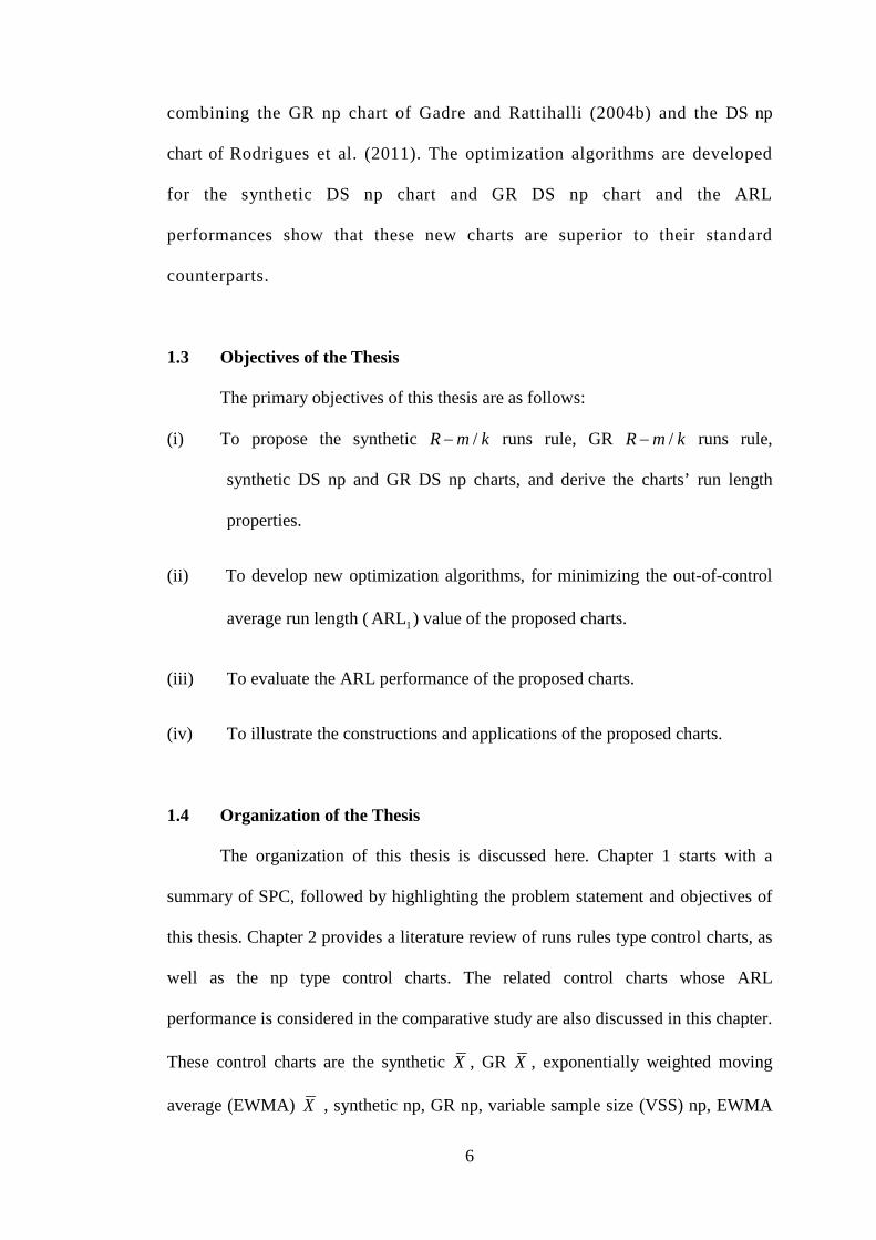
1.3 Objectives of the Thesis

The primary objectives of this thesis are as follows:

(i) To propose the synthetic /R m k− runs rule, GR /R m k− runs rule,

synthetic DS np and GR DS np charts, and derive the charts’ run length

properties.

(ii) To develop new optimization algorithms, for minimizing the out-of-control

average run length ( 1ARL ) value of the proposed charts.

(iii) To evaluate the ARL performance of the proposed charts.

(iv) To illustrate the constructions and applications of the proposed charts.

1.4 Organization of the Thesis

The organization of this thesis is discussed here. Chapter 1 starts with a

summary of SPC, followed by highlighting the problem statement and objectives of

this thesis. Chapter 2 provides a literature review of runs rules type control charts, as

well as the np type control charts. The related control charts whose ARL

performance is considered in the comparative study are also discussed in this chapter.

These control charts are the synthetic X , GR X , exponentially weighted moving

average (EWMA) X , synthetic np, GR np, variable sample size (VSS) np, EWMA

7

np, cumulative sum (CUSUM) np and CUSUM np with fast initial response (FIR)

charts. The ARL performance measure will also be discussed in this chapter.

Moreover, Chapter 2 explains the run length properties of the /R m k− runs rule, DS

np, synthetic X and synthetic np, GR X and GR np charts.

Chapter 3 discusses the constructions and optimal designs of the proposed

synthetic /−R m k runs rule and GR /R m k− runs rule charts in detail. Illustrative

examples to show the applications of the synthetic /R m k− runs rule and GR

/R m k− runs rule charts will also be discussed in Chapter 3. In Chapter 4, the

constructions and optimal designs of the proposed synthetic DS np and GR DS np

charts are explained. Chapter 4 also demonstrates the applications of the synthetic

DS np and GR DS np charts using illustrative examples.

The ARL performance comparison of the proposed synthetic /R m k− runs

rule and GR /R m k− runs rule charts and their existing counterparts (discussed in

Section 2.4) is presented in Chapter 5. In addition, Chapter 5 discusses the ARL

performance comparison of the synthetic DS np and GR DS np charts and their

existing counterparts (discussed in Section 2.5). Finally, the findings and

contributions of this thesis, as well as recommendations for future research are

summarized in Chapter 6.

Numerous optimization and simulation programs written in the Statistical

Analysis System (SAS) and MATLAB software are presented in Appendices A, C, D

and E. These programs are written to compute the optimal parameters and ARL

properties of the /R m k− , synthetic /R m k− , GR /R m k− , synthetic X , GR X ,

EWMA X , single sampling (SS) np, DS np, synthetic np, GR np, VSS np, EWMA

np, CUSUM np and CUSUM (FIR) np charts. The Markov chain model to obtain the

ARLs of 4 / 5R − , EWMA X , VSS np , EWMA np and CUSUM np charts are

8

given in Appendix B. The additional results for the performance comparison of the

synthetic /R m k− and GR /R m k− (synthetic DS np and GR DS np) charts with

existing charts are given in Appendix F (Appendix G).

CHAPTER 2 LITERATURE REVIEW

2.1 Introduction

In this chapter, we will review all the existing literature related to this study.

The Shewhart X control chart, which can signal an out-of-control status when a

sample point is plotted beyond the three-sigma limits, is widely used in

manufacturing and service industries due to its simplicity to shop floor personnel.

However, the Shewhart X control chart is known to be effective for detecting large

process mean shifts but relatively insensitive towards small and moderate process

mean shifts. In order to overcome this problem, the use of runs rules have been

suggested in the literature. In Section 2.2, we will discuss runs rules type control

charts in detail. The relevant literature review on np type control charts is discussed

in Section 2.3, which includes the SS np and DS np control charts.

Several related control charts that are considered in the ARL performance

comparison in Chapter 5 are also discussed in this chapter. Section 2.4 discusses the

relevant variables control charts, i.e. synthetic X , GR X and EWMA X control

charts. The relevant attributes control charts, i.e. synthetic np, GR np, VSS np,

EWMA np, CUSUM np and CUSUM (FIR) np charts are discussed in Section 2.5.

Section 2.6 defines and gives some discussions on the ARL as a performance

measure of a chart.

2.2 Runs Rules Type Control Charts

There were numerous studies on runs rules type control charts and their use in

SPC can be traced back to the 1940s. Shewhart (1941) proposed additional test using

runs rules to enhance the sensitivity of the Shewhart X chart towards small process

9

mean shifts. Koutras et al. (2007) pointed out that some authors proposed quality

control charts which use acceptance or rejection principle of extended sequences of

points that plot within or beyond the control limits, while others enhanced the basic

Shewhart X chart with supplementary runs rules (see Mosteller, 1941; Wolfowitz,

1943). Later on, Weiler (1953) discussed the use of runs to control the mean of a

process by proposing the k-of-k runs rule that signals when k successive points plot

beyond the control limits. Furthermore, Page (1955) studied process inspection

methods using control charts with warning limits and introduced four types of runs

rules charts. He also introduced a Markov chain approach to calculate the exact run

length distribution of the chart’s performance.

To improve the sensitivity of the Shewhart X chart, Western Electric (1956)

presented a set of decision rules based on runs and scans. This set of decision rules

signal an out-of-control if at least one of these events happen(s) (Western Electric,

1956)

(i) A point falls outside the three-sigma limits.

(ii) Two out of three successive points fall outside the two-sigma warning limits.

(iii) Four out of five successive points fall outside the one-sigma limits or beyond.

(iv) Eight successive points fall on the same side of the center line.

Moore (1958) also proposed run-based acceptance sampling plans similar to

Page (1955). Roberts (1958) noted that the use of supplementary runs rules without

compensating zone limits will increase the number of false alarms. He also

introduced the term “zone chart” to define a control technique that uses runs rules in

a Shewhart X chart. Westgard and Groth (1979) studied the power functions for

some control charts and concluded that the use of runs rules can lead to an increase

in the false alarm rate.

10

Wheeler (1983) calculated the power function of a one-sided Shewhart X

chart with four sets of supplementary runs rules to detect shifts in the process mean

and presented them in tables. He found that the use of runs rules increases the

sensitivity of the Shewhart X chart towards small process mean shifts. Nelson (1984)

discussed the advantages and disadvantages of the Shewhart X chart supplemented

with runs rules and concluded that the use of multiple decision rules at the same time

is discouraged as it will have an impact on the computations of the probabilities of

Type I and Type II errors. Moreover, Nelson (1985) recommended that the test based

on decision rules should be viewed as some practical rules for action instead of tests

with specific probabilities linked with them.

Champ and Woodall (1987) provided an easy method that uses the Markov

chain approach to get the exact run length properties of the Shewhart X chart with

runs rules. They also concluded that the use of simultaneous tests will increase the

power of the control chart and lead to an increase in the false alarm rates. Palm (1990)

provided some tables of the ARL and percentiles of the run length of the Shewhart

X charts supplemented with common runs rules. Champ and Woodall (1990) wrote

a Fortran computer program using the Markov chain method to calculate the run

length properties of the Shewhart X chart supplemented with runs rules and pre-

determined control limits. Besides, Walker et al. (1991) obtained the false alarm rate

of the Shewhart X chart with supplementary runs rules using a simulation study and

concluded that the false alarm rate is quite high, especially when the number of

multiple use of runs rules or number of subgroups increases. They also showed that

their simulation results draw similar conclusion to the results of Champ and Woodall

(1987).

11

Hurwitz and Mathur (1992) introduced a very simple two-of-two runs rule

which can signal if two successive points fall outside the control limits. Champ

(1992) studied the cyclic steady-state run length distribution of the Shewhart X

chart with supplementary runs rules by combining the Markov chain technique of

Champ and Woodall (1987) with the cyclic steady-state distribution of Crosier

(1986). Alwan et al. (1994) investigated the ARL of runs rules type control charts

when autocorrelation is present. Lowry et al. (1995) attempted to improve the

sensitivity of the Shewhart R- and S-charts to monitor process dispersion by

incorporating the standard Western Electric Company runs rules but the results

turned out to be poor. They suggested alternative runs rules that will give the same in

control ARL performance as the standard Shewhart chart with runs rules, and

concluded that all these runs rules were ineffective to decrease the dispersion of a

process.

Das and Jain (1997) studied the economic design of the Shewhart X chart

with supplementary runs rules. Champ and Woodall (1997) proposed the Shewhart

X chart with a multiple set of runs rules and computed their false alarm signal

probabilities, which are important when selecting runs rules based on the false alarm

rate. Shmueli and Cohen (2003) presented a new technique for computing the run

length distribution of the Shewhart X chart supplemented with runs rules by using

run-length generating function to extract the probability function. Based on their

technique to compute the run length distribution, they managed to compare the entire

run length distribution of common runs rules and concluded that the study based on

the entire run length distribution provides more information than the study based on

the ARL only. Fu et al. (2003) introduced a generalized method based on the Markov

chain imbedding approach to calculate the run length distribution of various

12

Shewhart X charts based on a simple rule or on the compound rules. Zhang and

Castagliola (2010) proposed runs rules X chart when the process parameters are

estimated. They examined the performance of the runs rules X chart using the

Markov chain model and compared them with the case where the process parameters

are assumed known and concluded that their run length properties are quite different.

2.2.1 Standard m-of-k ( /m k ) Runs Rules Control Chart

Western Electric (1956) proposed two m-of-k ( /m k ) runs rules, which are

the 2/3 and 4/5 rules. The 2/3 rule signals an out-of-control when two out of three

successive points plot beyond the two-sigma warning limits, while the 4/5 rule

signals an out of control when four out of five successive points plot beyond the one

sigma limits. Derman and Ross (1997) proposed slightly different 2/2 and 2/3 rules.

For the first rule, an out-of-control signal is given if two successive points plot

outside either of the control limits, while for the second rule, an out-of-control is

signalled if any two out of three successive points are above, or below, either control

limits. Klein (2000) presented more powerful 2/2 and 2/3 rules having symmetric

UCL and LCL. His 2/2 rule signals an out-of-control if two successive points plot

either above the UCL or below the LCL, whereas his 2/3 rule signals an out-of-

control if two out of three successive points are plotted either above the UCL or

below the LCL. Klein (2000) designed his 2/3 rule based on the Markov chain

approach to compute the UCL and LCL that give a desired 0ARL . The results

showed that the ARL performance of his runs rules chart is better than the Shewhart

X chart up to mean shifts of 2.6 standard deviations. Khoo (2003) provided detailed

steps to design control charts with supplementary runs rules and conducted a

simulation study of the 2/2, 2/3, 2/4, 3/3 and 3/4 rules for different choices of 0ARL s

13

and concluded that the 3/4 rule has the best ARL performance. A typical m k/ runs

rule chart signals an out-of-control if m-of-k successive points are plotted either

above the /UCLm k or below the /LCLm k .

2.2.2 Improved m-of-k ( − /I m k ) Runs Rules Control Chart

By combining the classical 1/1 rule with the 2/2 and 2/3 rules, Khoo and

Ariffin (2006) proposed the improved m-of-k rules (denoted by /I m k− , where

2m = and k = 2 or 3). The /I m k− runs rule will signal an out-of-control if either a

point falls beyond the outer control limits or if m-of-k successive points lie between

the inner and outer control limits. The 2 / 2I − and 2 / 3I − rules provide superior

ARL performance to the corresponding 2/2 and 2/3 rules of Klein (2000) for

detecting large process mean shifts, while maintaining the same sensitivity for the

detection of small and moderate process mean shifts. Acosta-Mejia (2007) studied

the ARL performance of the /I k k− and / ( 1)I k k− + rules for various k values

and concluded that these rules have improved performances for detecting small mean

shifts compared with the Shewhart X chart, but the former rules are comparable to

the latter chart for detecting large mean shifts.

To use the /I m k− runs rule, we design the Shewhart X chart with a center

line ( )/CLI m k− and two sets of symmetrical control limits, i.e. inner control limits

( )1 ( / ) 1 ( / )LCL , UCLI m k I m k− − and outer control limits ( )2 ( / ) 2 ( / )LCL , UCLI m k I m k− − ,

which satisfy 2 ( / ) 1 ( / ) / 1 ( / ) 2 ( / )LCL LCL CL UCL UCL− − − − −< < < <I m k I m k I m k I m k I m k . For

example, consider the case where 2k ≥ and 2 m k≤ ≤ . Here, the /I m k− runs rule

signals an out-of-control if

(i) a single sample point is plotted above 2 ( / )UCL −I m k or below 2 ( / )LCL −I m k , or

14

(ii) m out of k successive points fall between ( )1 ( / ) 1 ( / )UCL LCLI m k I m k− − and

( )2 ( / ) 2 ( / )UCL LCLI m k I m k− − .

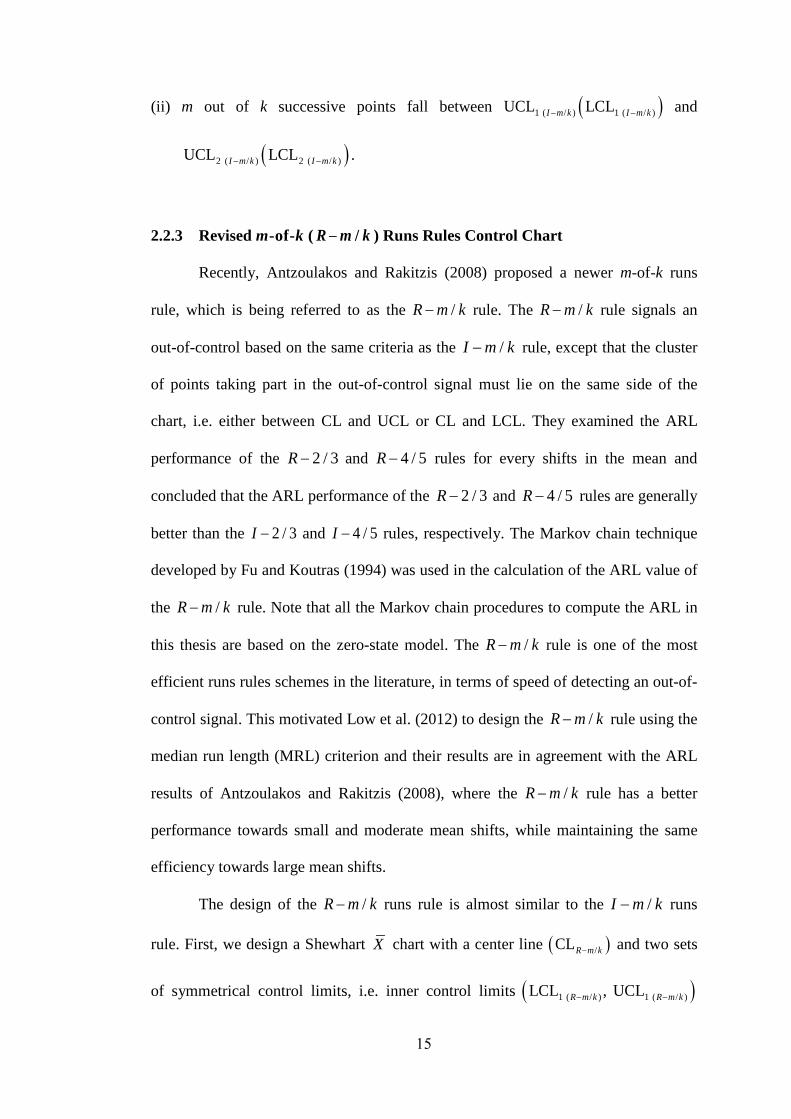
2.2.3 Revised m-of-k ( − /R m k ) Runs Rules Control Chart

Recently, Antzoulakos and Rakitzis (2008) proposed a newer m-of-k runs

rule, which is being referred to as the /R m k− rule. The /R m k− rule signals an

out-of-control based on the same criteria as the /I m k− rule, except that the cluster

of points taking part in the out-of-control signal must lie on the same side of the

chart, i.e. either between CL and UCL or CL and LCL. They examined the ARL

performance of the 2 / 3R − and 4 / 5R − rules for every shifts in the mean and

concluded that the ARL performance of the 2 / 3R − and 4 / 5R − rules are generally

better than the 2 / 3I − and 4 / 5I − rules, respectively. The Markov chain technique

developed by Fu and Koutras (1994) was used in the calculation of the ARL value of

the /R m k− rule. Note that all the Markov chain procedures to compute the ARL in

this thesis are based on the zero-state model. The /R m k− rule is one of the most

efficient runs rules schemes in the literature, in terms of speed of detecting an out-of-

control signal. This motivated Low et al. (2012) to design the /R m k− rule using the

median run length (MRL) criterion and their results are in agreement with the ARL

results of Antzoulakos and Rakitzis (2008), where the /R m k− rule has a better

performance towards small and moderate mean shifts, while maintaining the same

efficiency towards large mean shifts.

The design of the /−R m k runs rule is almost similar to the /−I m k runs

rule. First, we design a Shewhart X chart with a center line ( )/CLR m k− and two sets

of symmetrical control limits, i.e. inner control limits ( )1 ( / ) 1 ( / )LCL , UCLR m k R m k− −

15

and outer control limits ( )2 ( / ) 2 ( / )LCL , UCL ,R m k R m k− − which satisfy 2 ( / )LCL R m k− <

1 ( / )LCL R m k− < /CLR m k− < 1 ( / )UCL R m k− < 2 ( / )UCL R m k− . Consider the case where 2k ≥

and 2 m k≤ ≤ . Here, the /−R m k runs rule signals an out-of-control if

(i) a single sample point is plotted above 2 ( / )UCL −R m k or below 2 ( / )LCL −R m k , or

(ii) m out of k consecutive sample points fall between ( )1 ( / ) 1 ( / )UCL LCLR m k R m k− − and

( )2 ( / ) 2 ( / )UCL LCLR m k R m k− − , and the group of points contributing to the out-of-control

signal fall between /CL −R m k and ( )2 ( / ) 2 ( / )UCL LCLR m k R m k− − .

For the design of the /R m k− runs rule, we start by setting the desired value for

the 0ARL , i.e. τ , followed by setting the width constant of the outer control limit,

2d . After that, we determine the inner control limit constant, 1d so that the desired

value of τ is obtained. The outer control limits are computed using

2 ( / ) 2 ( / )UCL / LCLR m k R m k− − = 00 2 ,σμ ± d

n and the inner control limits are calculated

using 1 ( / ) 1 ( / )UCL / LCLR m k R m k− − = 00 1

σμ ± dn

, where n is the sample size, 0µ is

the in-control mean and 0σ is the in-control standard deviation.

As the /R m k− runs rule chart will be considered in the performance

comparison in Chapter 5, it is useful to study its Markov chain method. The

Shewhart X chart with center line ( )/CLR m k− , outer control limits

( )2 ( / ) 2 ( / )LCL , UCLR m k R m k− − and inner control limits ( )1 ( / ) 1 ( / )LCL , UCLR m k R m k− − ,

based on the /R m k− runs rule is explained below. This /R m k− runs rule chart

can be divided into five intervals as follows (Antzoulakos and Rakitzis, 2008):

16

17

(i) Interval 1 represents the area between the 1 ( / )UCL R m k and the 2 ( / )UCL R m k .

(ii) Interval 2 represents the area between the /CL R m k and the 1 ( / )UCL R m k .

(iii) Interval 3 represents the area between the 1 ( / )LCL R m k and the /CL R m k .

(iv) Interval 4 represents the area between the 2 ( / )LCL R m k and the 1 ( / )LCL R m k .

(v) Interval 5 represents the area beyond the 2 ( / )LCL R m k and the 2 ( / )UCL R m k .

Let 1 0 0 be the size of the mean shift, where 1 is the

out-of-control mean. When /CL R m k of this chart is fixed as zero and symmetrical

outer and inner limits are used, the probabilities 1p , 2p , 3p , 4p and 5p for a sample

point to fall in intervals 1, 2, 3, 4 and 5, respectively, are (Antzoulakos and Rakitzis,

2008)

1 2 1 ,p d d (2.1)

2 1 1,p d (2.2)

3 1 ,p d (2.3)

4 2 1p d d (2.4)

and

5 1 2 3 41 ,p p p p p (2.5)

where . denotes the cumulative distribution function (cdf) of the standard normal

distribution.

For illustration, we consider the case of the 2 / 3R runs rule to describe

how the Markov chain approach works. Let { tZ , t ≥ 1} be a sequence of independent

and identically distributed (iid) trials taking the value in set A = {1, 2, 3, 4, 5}, and

( ) t iP Z i p , where i = 1, 2, …, 5. Consider the composite pattern

1D = {11, 121, 44, 434, 5}, (2.6)

which includes all the different ways to get an out-of-control signal. Here, 11

represents two successive samples falling in interval 1.

The steps to obtain the Markov chain states for the 2 / 3−R runs rule are as

follows (Low et al., 2012):

Step 1. Write down all the elements in the composite pattern 1D .

Step 2. Decompose each element in composite pattern 1D into its basic

states. For instance, element 121 can be decomposed into “1” and

“12”. After decomposing all the elements in the composite pattern

1D , we will get the basic states of “1”, “12”, “4” and “43”.

Step 3. Represent the out-of-control state as “AS” = {“11”, “121”, “44”, “434”,

“5”}.

Step 4. Identify the missing basic state not found in Step 2. In this case, it is the

basic state for regions 2 or 3, that is “2 or 3”.

Step 5. Merge all the basic states obtained in Steps 2 and 4 to get the in-control

states of “2 or 3”, “1”, “12”, “4” and “43”.

After getting all the in-control states for the Markov chain model,

the transition probability matrix (tpm) for the transient states, 1R is

constructed as shown in Table 2.1. Each entry denotes the transition

probability from state i to state j.

18

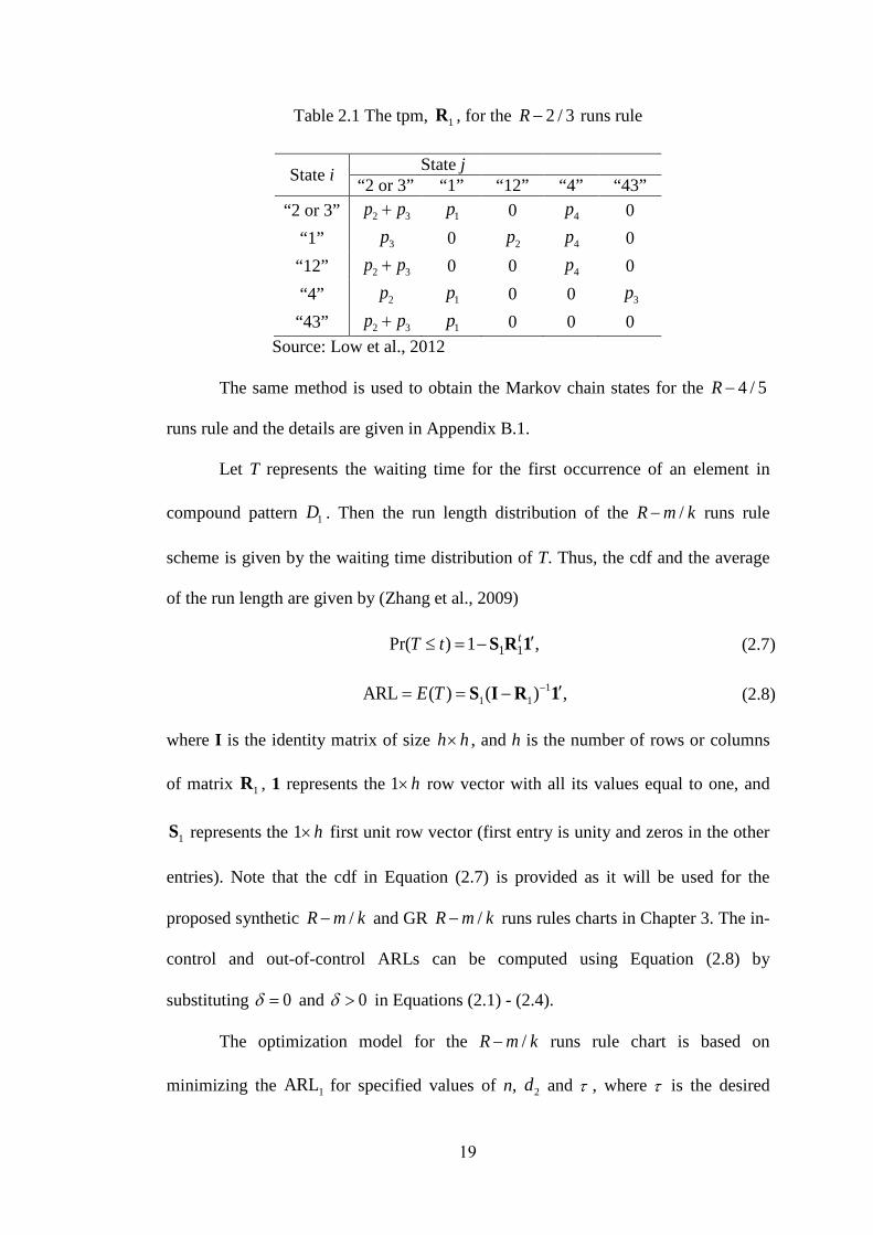
Table 2.1 The tpm, 1R , for the 2 / 3−R runs rule

State i State j “2 or 3” “1” “12” “4” “43”

“2 or 3” 2 3+p p 1p 0 4p 0 “1” 3p 0 2p 4p 0 “12” 2 3+p p 0 0 4p 0 “4” 2p 1p 0 0 3p “43” 2 3+p p 1p 0 0 0

Source: Low et al., 2012

The same method is used to obtain the Markov chain states for the 4 / 5R −

runs rule and the details are given in Appendix B.1.

Let T represents the waiting time for the first occurrence of an element in

compound pattern 1D . Then the run length distribution of the /R m k− runs rule

scheme is given by the waiting time distribution of T. Thus, the cdf and the average

of the run length are given by (Zhang et al., 2009)

1 1Pr( ) 1 ,S R 1tT t ′≤ = − (2.7)

11 1ARL ( ) ( ) ,S I R 1E T − ′= = − (2.8)

where I is the identity matrix of size h h× , and h is the number of rows or columns

of matrix 1R , 1 represents the 1 h× row vector with all its values equal to one, and

1S represents the 1 h× first unit row vector (first entry is unity and zeros in the other

entries). Note that the cdf in Equation (2.7) is provided as it will be used for the

proposed synthetic /R m k− and GR /R m k− runs rules charts in Chapter 3. The in-

control and out-of-control ARLs can be computed using Equation (2.8) by

substituting 0δ = and 0δ > in Equations (2.1) - (2.4).

The optimization model for the /R m k− runs rule chart is based on

minimizing the 1ARL for specified values of n, 2d and τ , where τ is the desired

19

0ARL value. The optimization program for the 2 / 3R − and 4 / 5R − runs rules

charts written using the MATLAB software is given in Appendix A.1.

2.3 np Type Control Charts

The basic attribute control charts are the p, np, c and u charts. The p and np

charts are commonly used to monitor the fraction of non-conforming items while the

c and u charts are used to monitor the number of non-conformities. Moreover, the p

and np charts’ control limits and designs are based on the binomial distribution while

those of the c and u charts are based on the Poisson distribution (Woodall, 1997).

The np control chart is commonly used to detect increases in the fraction non-

conforming for attribute data. The sample fraction non-conforming, p is defined as

the ratio of the number of non-conforming units in the sample, 0e to the sample size,

n. The np chart is as effective as the p chart when the sample size n is constant, but

the np chart is easier to understand as it is based on the number of non-conforming

items (Montgomery, 2009). Haridy et al. (2012) noted that the common use of the np

chart and other attribute charts is attributable to several factors, such as the relative

simplicity of handling attribute quality characteristics, the capability of checking

multiple quality requirements, the ease to communicate between people at different

levels and the prevalence of count data in many non-manufacturing sectors. A

process is considered to be in-control if SS np 0 SS npLCL UCLe≤ ≤ , where SS npLCL and

SS npUCL are the lower and upper control limits of the SS np chart, respectively.

Otherwise, if 0 SS np< LCLe or 0 SS np> UCLe the process has gone out-of-control. For

the case of 0 SS np< LCLe , a decrease in p is signalled, while for the case of

20

0 SS np> UCLe , an increase in p is signalled. Note that the standard np chart is referred

to as the SS np chart in this thesis.

Various economic design models for the p chart and np chart have been

suggested from the 1970 onwards. Montgomery et al. (1975) presented the economic

design of fraction defective control charts by developing an expected cost model for

the defective control chart. Montgomery and Heikes (1976) furthered the study of

economic design of fraction defective control charts by investigating the optimal

design of fraction defective control charts using both the Markov and non-Markov

models. Chiu (1976) studied the economic design model of np chart for production

processes which have an in-control state but such processes may fall into either one

of the few out-of-control states such that each state is related to an assignable cause.

Chiu (1977) also examined how errors in estimation affect the optimal cost control

scheme using the np chart.

Duncan (1978) presented the minimum cost p chart by converting the

minimum cost designs of np chart into p chart and found that larger samples taken

less often are required in the detection of small shifts. Gibra (1978) developed two

production models using easy search procedure to find the optimal parameter of an

np chart with minimum cost function and showed how the models can be used using

illustrative examples. Moreover, Gibra (1981) extended the two models to monitor

industrial process subject to a multiplicity of assignable causes and showed that the

proposed complex multiple cause model can be approximated by a “similar” single

cause model. Sculli and Woo (1982) presented a simulation method to design the np

chart which is useful in the control of a manufacturing process.

In addition, Sculli and Woo (1985) developed two models that allow the

product quality to decline to a lower level without the detection of an out-of-control

21

state and they can be used in conditions where the out-of-control causes and the

proportion of defectives are unknown. Williams (1985) developed an economic

design cost model for the np chart using curtailed sampling plans and showed that

the proposed curtailed sampling plans reduce cost when compared with traditional

sampling plans. Collani (1989) developed a simple method to construct an

approximate optimal economic design of the np chart. Wang and Chen (1995)

considered an economic design of the np chart under fuzzy environment which

fulfilled the Type I and II errors and used a heuristic approach to get the solution.

2.3.1 Single Sampling (SS) np Control Chart

Control charts for attribute data were first suggested by Shewhart (1926 and

1927). Some early works for improving the technique of the p and np charts were

made by Jenett and Welch (1939), Wescott (1947), Howell (1949), Olds (1956),

Folks et al. (1965) and Larson (1969). Nelson (1983) presented a supplementary test

for a p control chart which includes counting the number of consecutive occurrences

of non-conforming items in a subgroup. To control process with low defective rates,

Goh (1987) developed an alternative charting technique based on exact probability

calculations and showed that the new p chart is more effective compared with the

standard p chart for low defective production. Bissell (1988) presented a simple way

for computing the control charts’ limits for attributes, which include the p, np and c

charts. To improve the effectiveness of the np chart, Vaughan (1992) presented a

variable sampling interval (VSI) np chart, which allows each sample to be taken at

different intervals depending on the power of the sampling procedure.

Schwertman and Ryan (1997) presented a Fortran program that enabled the

user to find the optimal control limits for a p, np, c or u chart by assuming that all the

22

parameter values are known. Jolayemi (2002) developed models of the np chart with

three and four control regions and concluded that an increase in the number of

control regions will decrease the discriminatory power of the np chart, and vice versa.

Laney (2002) proposed a p chart which solves the problem of the traditional p chart

which requires the assumption that the mean of the distribution is constant over time,

which is not always true. Wu et al. (2006) proposed an algorithm to optimize the np

chart with curtailment and found that the proposed optimal np chart with curtailment

can decrease the out-of-control average time to signal (ATS) by almost 50% on the

average compared with the traditional np chart.

The SS np chart is a conventional np control chart and it is constructed based

on the number of non-conforming items. As it is important to detect an increase in

the fraction nonconforming p, only the upper sided standard np chart is usually

considered. This SS np chart signals an out-of-control when 0 SS npUCLe ≥ , where 0e

is the number of non-conforming items in a sample of size n and SS npUCL is a pre-

defined upper control limit of the SS np chart. Let P be the probability that the

number of non-conforming items 0e is less than SS npUCL of the SS np chart. Then

(Rodrigues et al., 2011)

( ) ( )SS np

0

0

0

UCL

0 SS np0 0

Pr UCL 1 e

e

e nPn

e p pe

−

=

= < = −

∑ , (2.9)

where ⌊ ⋅ ⌋ denotes the ‘biggest integer less than or equal to its argument’.

The ARL of the SS np chart is obtained as

1ARL =1 P−

. (2.10)

The in-control and out-of-control ARLs are computed using Equation (2.10) when

0=p p and 1,=p p respectively, where 0p denotes the in-control fraction of non-

23

conforming items while 1p denotes the out-of-control fraction of non-conforming

items.

The optimal design of the SS np chart is based on finding an appropriate

SS npUCL such that 0ARL τ≥ for pre-determined n and τ values. The MATLAB

optimization program written based on this model is presented in Appendix A.2.

2.3.2 Double Sampling (DS) np Control Chart

Wu and Wang (2007) proposed a new double inspection np chart which uses

a double inspection method to determine the process status. The first inspection

determines the process status as either in-control or out-of-control while the second

inspection determines the location of a specific non-conforming item in the sample.

Rodrigues et al. (2011) extended the idea of Wu and Wang (2007) by proposing the

DS np chart which gives superior ARL performance to the traditional np chart. The

DS np chart can also be used to lower the average sample size (ASS) without

affecting the ARL performance. The DS np chart of Rodrigues et al. (2011) was

developed to detect assignable causes that result in an increase in p. As such, this DS

np chart is defined with the lower control limit ( )DS npLCL set as zero. To apply the

DS np chart, a first sample is drawn and examined at a fixed sampling interval. Using

the results taken from the first sample, the sampling either stops for a conclusion

about the process to be made or an additional second sample is drawn and examined,

followed by making a conclusion about the process using the combined information

from both samples.

The following discussion explains the DS np chart of Rodrigues et al.

(2011). Assume that the DS np chart is applied to monitor a process which

is binomially distributed with parameters n and p. Then the DS np chart

24

PROPOSED SYNTHETIC AND GROUP RUNS CONTROL …

Documents

Transcript of PROPOSED SYNTHETIC AND GROUP RUNS CONTROL …