Proposed Approach for Developing Lead Dust … · Proposed Approach for Developing Lead Dust Hazard...
82
SAB CONSULTATION DRAFT – July 6-7, 2010 Proposed Approach for Developing Lead Dust Hazard Standards for Commercial and Public Buildings June 3, 2010 Office of Pollution Prevention and Toxics U.S. Environmental Protection Agency Washington, D.C.
Transcript of Proposed Approach for Developing Lead Dust … · Proposed Approach for Developing Lead Dust Hazard...

SAB CONSULTATION DRAFT – July 6-7, 2010
Proposed Approach for Developing Lead Dust Hazard Standards for Commercial and Public Buildings
June 3, 2010
Office of Pollution Prevention and Toxics
U.S. Environmental Protection Agency
Washington, D.C.

SAB CONSULTATION DRAFT – July 6-7, 2010
TABLE OF CONTENTS
1. Introduction............................................................................................................................. 6
1111
11
11
12
12
13
1414
15
16
19
19
24
25
2727
27
28
29
29
30
3232
33
33
3636
37
2. Target Blood Lead Concentration....................................................................................... 2.1. Selection of Endpoints ......................................................................................................
2.1.1. Children under age 6...................................................................................................
2.1.2. Adults..........................................................................................................................
2.2. Selection of Target Blood Lead Concentrations...............................................................
2.2.1. Children under age 6...................................................................................................
2.2.2. Adults..........................................................................................................................
3. Environmental Media and Exposure Concentrations....................................................... 3.1. Estimating Distributions of Concentrations in Each Microenvironment..........................
3.2. Estimating Media Concentrations from Distributions ......................................................
3.3. Converting Dust Lead Loading to Dust Lead Concentration ...........................................
3.4. Characterizing Exposure Variables...................................................................................
3.4.1. Human activity patterns ..............................................................................................
3.4.2. Other exposure variables.............................................................................................
3.5. Estimating Exposure Concentrations................................................................................
4. Estimation of Blood Lead Levels ......................................................................................... 4.1. Children under age 6.........................................................................................................
4.1.1. Overview of blood lead models for children ..............................................................
4.1.2. IEUBK ........................................................................................................................
4.2. Adults................................................................................................................................
4.2.1. Overview of blood lead models for adults..................................................................
4.2.2. Leggett model .............................................................................................................
5. Application of the Model for Estimating Hazard Standards............................................ 5.1. Creating the Target Loading-to-Blood-Lead Response Surface.......................................
5.2. Estimating the Candidate Hazard Standard Using the Response Surface ........................
5.3. Sensitivity Analysis ..........................................................................................................
6. Data Needs ............................................................................................................................. 6.1.1. Media concentrations for residences...........................................................................
6.1.2. Media concentrations for public and commercial buildings.......................................
ii

SAB CONSULTATION DRAFT – July 6-7, 2010
6.1.3. Media concentrations near roadways.......................................................................... 37
37
38
39
45
6.1.4. Media concentrations outdoors ...................................................................................
6.1.5. The relationship between window sill and floor exposures........................................
6.1.6. Inputs to the blood lead models ..................................................................................
7. References..............................................................................................................................
Appendix A. Loading to Concentration Conversion Methods ............................................ A-1
iii

SAB CONSULTATION DRAFT – July 6-7, 2010
LIST OF TABLES Table 3-1. Media Concentration Distributions Needed for the Commercial and Public
Building Hazard Standard Approach............................................................................... 15
23
24
Table 5-1. Key Input Variables or Variable Groups Sampled in the Public and Commercial Buildings Model ............................................................................................ 33
37
41
Table 3-2 Children’s Time Spent in Selected Microenvironments, by Age..........................
Table 3-3. Adults’ Time Spent in Selected Microenvironments, by Age Group..................
Table 6-1. AQS Monitor Objective Codes ...............................................................................
Table 6-2. Proposed Blood Lead Model Input Values............................................................
iv

SAB CONSULTATION DRAFT – July 6-7, 2010
LIST OF FIGURES Figure 1-1. Overview of Approach for Developing Hazard Standards for Commercial and Public
Buildings ..................................................................................................................... 8
38
39
Figure 6-1. Regression Relationship between Ln(Sill) and Ln(Floor) for the HUD Data ..........
Figure 6-2. Regression Relationship between Ln(Sill) and Ln(Floor) for the Rochester Data ...
v

SAB CONSULTATION DRAFT – July 6-7, 2010
1. Introduction 1
2 3 4 5
6 7 8 9
10 11 12 13
14 15 16 17 18 19 20 21
22 23
24 25 26 27 28 29
30 31 32
33 34 35
36 37 38
39
40
Section 402(c)(3) of TSCA directs EPA to revise the regulations promulgated under TSCA section 402(a), i.e., the Lead-based Paint Activities Regulations, to apply to renovation or remodeling activities in target housing, public buildings constructed before 1978, and commercial buildings that create lead-based paint hazards. In April 2008, EPA issued the final
Renovation, Repair and Painting Rule (RRP Rule) under the authority of section 402(c)(3) of TSCA to address lead-based paint hazards created by renovation, repair, and painting activities that disturb lead-based paint in target housing and child-occupied facilities (USEPA, 2008a). The term ‘‘target housing’’ is defined in TSCA section 401 as any housing constructed before 1978, except housing for the elderly or persons with disabilities (unless any child under age 6 resides or is expected to reside in such housing) or any 0- bedroom dwelling. Under the RRP Rule, a child-occupied facility is a building, or a portion of a building, constructed prior to 1978, visited regularly by the same child, under 6 years of age, on at least two different days within any week
(Sunday through Saturday period), provided that each day’s visit lasts at least 3 hours and the combined weekly visits last at least 6 hours, and the combined annual visits last at least 60 hours. The RRP Rule establishes requirements for training renovators, other renovation workers, and dust sampling technicians; for certifying renovators, dust sampling technicians, and renovation firms; for accrediting providers of renovation and dust sampling technician training; for renovation work practices; and for recordkeeping. Interested States, Territories, and Indian Tribes may apply for and receive authorization to administer and enforce all of the elements of the RRP Rule.
Shortly after the RRP Rule was published, several petitions were filed challenging the rule. These petitions were consolidated in the Circuit Court of Appeals for the District of Columbia
Circuit. On August 24, 2009, EPA entered into an agreement with the environmental and children’s health advocacy groups in settlement of their petitions (USEPA, 2009a). In this agreement, EPA committed to propose several changes to the RRP Rule. EPA also agreed to commence rulemaking to address renovations in public and commercial buildings, other than child-occupied facilities, to the extent those renovations create lead-based paint hazards. For these buildings, EPA agreed, at a minimum, to do the following:
• Issue a proposal to regulate renovations on the exteriors of public and commercial buildings other than child-occupied facilities by December 15, 2011 and to take final action on that proposal by July 15, 2013.
• Consult with EPA’s Science Advisory Board by September 30, 2011, on a methodology for evaluating the risk posed by renovations in the interiors of public and commercial buildings other than child-occupied facilities.
• Eighteen months after receipt of the Science Advisory Board’s report, either issue a proposal to regulate renovations on the interiors of public and commercial buildings other than child-occupied facilities or conclude that such renovations do not create lead-based
paint hazards.
6

SAB CONS
7
ULTATION DRAFT – July 6-7, 2010
1 2 3 4 5 6 7 8 9
10 11 12
13 14 15
16 17 18 19 20 21 22 23 24
25 26 27 28 29 30
31
32
The second step, Estimate Environmental Media and Exposure Concentrations, involves characterizing lead concentrations in relevant environmental media and using these data, in conjunction with information about human behavior patterns, to estimate lead exposures for the modeled populations. This step consists of three parts: selecting dust-lead levels for window sills and floors (candidate hazard standards), estimating environmental media concentrations, and estimating exposure concentrations.
The first step, Select Target Blood Lead Concentration, involves the selection of target blood lead levels for children and adults. For children, the proposed approach will focus on target blood lead levels that are associated with IQ effects in children; three target blood lead levels have been selected which are at the low end of the concentration-response curve. For adults, the proposed approach will focus on target blood lead levels that are associated with blood pressure effects in adults; several target blood lead levels have been selected which are at the low end of the concentration-response curve. The remaining steps of the approach will then be applied to estimate the candidate dust-lead levels (hazard standards) for floors and window sills that do not result in blood lead levels exceeding the target levels in children and adults.
In order to evaluate the potential risks associated with lead exposure due to renovations in public and commercial buildings, and the potential need for regulations on these activities, it is first necessary to develop the hazard standards for lead dust on window sills and floors in public and commercial buildings; these become the standards to help inform the impact of renovation activities. These standards will identify dangerous levels of lead in paint and dust, and provide benchmarks on which to base remedial actions taken to safeguard children and the public from the dangers of lead. This document describes OPPT’s proposed approach for developing the dust-lead hazard standards for floors and window sills in commercial and public buildings. OPPT will consider hazard standards for children and adults, as there may be some public and commercial buildings which children are unlikely to visit. Figure 1-1 provides an overview of the approach for developing hazard standards for public and commercial buildings. The approach is made up of three primary steps:
• Select target blood lead concentration • Estimate environmental media and exposure concentrations; and • Estimate blood lead concentrations.

SAB CONS
8
ULTATION DRAFT – July 6-7, 2010
1 2
Figure 1-1. Overview of Approach for Developing Hazard Standards for Commercial and Public Buildings
3

SAB CONSULTATION DRAFT – July 6-7, 2010
• Select candidate hazard standard. For each selected potential blood lead level of 1 concern, an initial candidate hazard standard for floor dust loading will be selected and carried through the remaining steps of the approach. The candidate hazard standard for window sill dust loading will be calculated based on the candidate hazard standard for floor loading using an estimated relationship between floor dust and window sill dust loadings.
2 3 4 5 6
8 9
10 11 12 13 14
15 16 17 18 19 20 21 22
23 24 25 26 27
28 29 30 31 32 33 34 35 36 37 38 39 40 41 42
43 44
• Estimate environmental media concentrations. The approach uses total blood lead 7 concentrations, rather than incremental concentrations attributable to different hazard standards, and as such, it requires estimates of lead concentrations for all relevant environmental media, rather than only focusing on lead concentrations on floors and window sills. To account for the variability in lead concentrations in other environmental media in the U.S., the approach will apply Monte Carlo sampling of distributions of background lead. To simplify the approach, it is assumed that environmental media concentrations will not change with time.
• Estimate exposure concentrations. Exposure concentrations are estimated by combining information about the lead concentrations in different environmental media with information about where the populations of interest are located at different times, what activities they are engaged in, and other information about their behavior. Children under age 6 were selected for this approach because they are the focus of the residential RRP rule and are considered to be the most susceptible population for IQ effects resulting from lead exposure. Adults were selected to allow consideration of non-IQ-related effects from lead exposure, such as hypertension. .
Distributions of exposure variables for these populations are selected to roughly represent the range of exposures experienced in the U.S. by children under age 6 and adults. Therefore, environmental media concentrations are assumed to remain constant with time, while estimated exposure concentrations will change with children’s ages to reflect behavior differences in development.
The temporal patterns of exposure concentrations for children under age 6 will be developed using different exposure scenario variables for each year (0-1, 1-2, etc.). For adults, the temporal patterns will be developed using different exposure variables for each age range, which will be determined based on an analysis of adult activity patterns. These exposure variables will be defined by distributions and Monte Carlo sampling will be applied to select values from these distributions. Distributions of the exposure variables related to human activity (i.e., where they spend time and how long they spend in each location) are developed by analyzing human activity data from the Consolidated Human Activity Database (CHAD) (USEPA 2009b). Distributions of other exposure parameters (e.g., soil/dust ingestion rate, water ingestion rate) are developed by analyzing data included in EPA’s Child-Specific Exposure Factors Handbook (USEPA 2008b). For both populations, each age (for children under age 6) or age group (for adults) will be simulated separately to develop distributions of exposure concentrations for that age/age range, and the resulting distributions of lead exposure concentrations for all modeled ages/age ranges will serve as inputs to the blood lead modeling.
In the third step of the approach, Estimate Blood Lead Concentrations, the distributions of exposure concentrations will be used to estimate a distribution of blood lead concentrations for
9

SAB CONSULTATION DRAFT – July 6-7, 2010
1 2 3 4 5 6
7 8 9
10 11 12 13
14 15 16
each population associated with a candidate hazard standard. As discussed further below, for children under age 6, blood lead concentrations will be estimated using EPA’s Integrated Exposure Uptake Biokinetic Model for Lead in Children (IEUBK). For adults, blood lead concentrations will be estimated using the International Commission for Radiation Protection’s Age-specific Biokinetic Model for Lead (the Leggett model), which, unlike the IEUBK, is capable of being used for estimating blood lead levels in adults.
After sufficient Monte Carlo samples have been simulated to develop a stable distribution of blood lead concentrations for each population, the estimated percentile of blood lead concentrations will be compared to the target blood lead level. If the estimate does not match the target (within the specified tolerance), a different candidate hazard standard for floor dust will be selected and the remaining steps of the approach will be repeated. This process continues until candidate hazard standards for floor dust and window sill dust have been developed for each population and potential level of concern.
The subsequent sections of this document provide more detailed descriptions of the approach for commercial and public buildings (Sections 2 through 5) and present the key data needs for consideration prior to implementing the approach (Section 6).
10

SAB CONSULTATION DRAFT – July 6-7, 2010
2. Target Blood Lead Concentration 1
2.1. Selection of Endpoints 2 3 4 5 6
7
8 9
10 11 12 13 14 15 16 17 18 19 20 21 22 23 24 25
26 27 28 29 30 31 32
33
34 35 36 37 38 39 40 41 42
In addition to a general hazard standard for public and commercial buildings, EPA is considering deriving an “adult hazard standard” for public and commercial buildings unlikely to be visited by children. Therefore, both children under age 6 and adults are considered in the target endpoint selection.
2.1.1. Children under age 6 There is a strong consensus within the public health community that the adverse effects of lead exposure are greatest in children and that impairment of neurological development is the “critical effect” (the effect occurring at the lowest exposure levels) (USEPA 2006, CDC 2005, 2009a, Bellinger 2008, Lanphear et al. 2005). The intelligence quotient (IQ) is the most commonly measured neurodevelopmental endpoint in lead-exposed children, and blood lead is the most common exposure/dose metric in epidemiological studies. A number of recent studies (Canfield et al. 2003, Chiodo et al. 2004, Jusko et al. 2008, Lanphear et al. 2005, Miranda et al. 2007, Surkan et al. 2007, Téllez-Rojo et al. 2006) have reported decrements in IQ and other adverse effects at blood lead levels less than 10 µg/dL. It is generally agreed that no specific “threshold” blood lead level for adverse effects on IQ in children has been identified. In addition to IQ measures, there is rapidly accumulating evidence that lead also affects other aspects of neurological development, and that in many of these studies, these effects were also observed in children at blood lead levels less than 10 µg/dL. These studies are reviewed in USEPA (2006); more recent reports include an association between early lead exposure and increased incidence of ADHD (Nigg et al. 2008, 2010), ADHD coupled with other behavior problems (Roy et al. 2008), as well as additional observations of increased criminal behavior (Wright et al. 2008) and other behavioral problems in young children (Chen et al. 2007).
Although there are some uncertainties in using both blood lead as a measure of exposure and IQ changes as an outcome measure, it is more difficult to generalize the results of the more complex neurobehavioral effects identified above. Therefore, children’s IQ has been chosen as the primary critical endpoint for determining the potential blood lead levels of concern. In making this choice, it is recognized that IQ effects do not capture the entire spectrum of adverse neurological effects associated with lead exposure in children. Estimating decrements in IQ thus represents a lower bound on the overall adverse effects of lead exposures to children.
2.1.2. Adults While adult lead exposures are known to be associated with a range of adverse effects, (USEPA 2006), the best documented endpoints, and those that have been found to occur in populations with relatively low body burdens, are effects on the cardiovascular system. Increases in blood pressure levels or hypertension is a risk factor for various cardiovascular diseases. A large number of studies have found blood lead concentrations to be associated with varying degrees of blood pressure elevation in adults. A large meta-analysis of 31 U.S. and European studies of over 54,000 subjects (Nawrot et al. 2002) found a statistically significant relationship between blood lead levels and both systolic and diastolic blood pressure. The study found that a doubling
11

SAB CONSULTATION DRAFT – July 6-7, 2010
1 2 3 4 5 6 7 8 9
10 11 12
13 14 15 16 17 18 19
20
22 23 24 25 26 27 28 29
30 31 32 33 34 35 36 37 38 39
40 41 42 43
of blood lead concentration was on average associated with a 1.0 mm Hg increase in systolic blood pressure (95 percent confidence limits 0.5 – 1.4 mm Hg) and a 0.6 mm Hg increase in diastolic blood pressure (95 percent confidence limits 0.4 – 0.8 mm Hg). Many of the studies reviewed by Nawrot et al. (2002) included substantial proportions of subjects with blood lead levels less than 10 ug/dL and no evidence of a threshold for blood pressure effects was found in an accompanying regression analysis of these data. In addition, a more recent review of the blood lead-blood pressure/cardiovascular disease data (Navas-Acien et al. 2007) similarly concluded that there is a modest relationship between blood lead concentrations and hypertension, and that there appears to be no threshold for these effects. Similar results have been reported in various populations, including menopausal and perimenopausal women (Nash et al. 2003), workers (Weaver et al. 2008), and individuals with different ALAD genotypes (Scinicariello et al. 2010).
Although several studies have evaluated a variety of possible cardiovascular effects associated with blood lead (including coronary artery disease, angina pectoris, acute myocardial infarction, heart rhythm abnormalities, stroke, peripheral artery disease, and mortality from cardiovascular disease and stroke; see reviews in USEPA 2006, Navas-Acien et al. 2007), the particular effect that is likely to arise from elevated blood pressure remains uncertain. Therefore, blood pressure has been chosen as the endpoint for determining the potential blood lead levels of concern in adults.
2.2. Selection of Target Blood Lead Concentrations 21
2.2.1. Children under age 6 For purposes of this Approach, a distribution for a hypothetical child will be modeled around individual candidate hazard standards. Blood lead levels of 1, 2.5 and 5 µg/dL have been chosen in order to evaluate a range of potential hazard standards. These levels were chosen, in part, based on recent literature which shows that increases in children’s blood lead from 1 to 10 µg/dL result in a greater decrement in IQ score than increases from 10 to 20 µg/dL, or from 20 to 30 µg/dL (Lanphear et al. 2005; Canfield et al. 2003; Schwartz 1994). This finding indicates a steeper dose-response relationship at blood lead levels less than 10 µg/dL.
Several different models relating various blood lead metrics (lifetime, concurrent, peak and early childhood) to IQ test results were reported in Lanphear et al. (2005). These models predicted a wide range of IQ changes for given blood lead concentrations. Log-linear models relating IQ changes to all blood lead metrics were developed and indicated that the relationships between IQ change and blood lead are curved, with steeper slopes at low blood lead levels. They also fit piecewise models (consisting of separate linear fits for different blood lead concentration ranges) to several of the blood lead metrics. The report presented the results developed for the concurrent blood lead metric, but EPA (U.S.EPA Activity-related Communication 2007) also obtained the relevant piecewise models for lifetime average blood lead concentrations based on the same data set.
For the blood lead metric, this approach is considering using both the lifetime and concurrent blood lead metrics. The peak blood lead metric was considered for this approach but ultimately not selected given the exposure scenario under consideration, which involved a relatively low-level, chronic exposure for the duration of the exposure period. Given that the approach does not
12

SAB CONSULTATION DRAFT – July 6-7, 2010
1 2 3 4 5 6 7 8 9
10 11 12 13 14 15 16 17 18 19 20 21
22 23 24
25
26
include time-varying media concentrations, concurrent blood lead measures could be preferred because they would involve calculating an average for ages 5 or 6 years, which might result in higher blood lead levels than the lifetime average because it would allow for maximum accumulation of lead in the body. On the other hand, exposures are likely to be highest during the first two years of life, based on behavior patterns and amount of time spent in the residence, and as a result the lifetime average could be higher than the concurrent concentration. For this approach, it is proposed that both metrics be calculated for each candidate hazard standard and that the metric resulting in the overall higher blood lead level be selected to provide a basis for standards presentation.
2.2.2. Adults This approach will use available blood lead-blood pressure relationships to select potential blood lead levels for consideration for the hazard standard for adults in public and commercial buildings. These levels have been selected in a manner consistent with that used to select the levels considered for children under age 6; that is, the available epidemiological data have been used to determine a lower-end range of adverse effects and several blood lead levels covering this range. Blood lead levels of 0.3, 1, 5, 10 and 20 µg/dL were chosen to evaluate a range of potential hazard standards using the Nawrot et al (2002) meta-analysis, which reported a two-fold increase in blood lead concentration associated with a 1.0 mm Hg rise in systolic pressure and a 0.6 mm Hg increase in diastolic pressure. These blood lead levels were chosen based on the range of average blood lead levels represented in the studies included in the meta analysis. A careful review of recent studies will be performed to ensure that there are no major new
findings that call the general results of that study into question, and sensitivity analyses can be used to derive defensible lower- and upper-bound risk estimates based on the Nawrot et al. (2002) statistical confidence limit estimates.
13

SAB CONSULTATION DRAFT – July 6-7, 2010
3. Environmental Media and Exposure Concentrations 1
2 3 4 5 6 7 8 9
10
12 13 14 15 16 17 18 19 20 21 22
23 24 25 26 27 28 29 30 31 32 33 34 35
36
Lead exposures are characterized in this approach by combining environmental media concentrations with exposure variable data (e.g., human activity data, ingestion rates, respiration rates). Distributions of environmental media concentrations are developed from the available literature for all microenvironments expected to contribute to lead exposures (e.g., floor dust, soil, air). These distributions are sampled using Monte Carlo techniques, the lead dust loadings are converted to lead dust concentrations (Appendix A), and the environmental media concentrations for the microenvironments are time-weight averaged using the activity pattern information and combined with other exposure variable data to estimate exposure concentrations. This process is described in detail below.
3.1. Estimating Distributions of Concentrations in Each Microenvironment 11 For each microenvironment of interest, distributions of dust lead concentrations, soil lead concentrations, and air lead concentrations are required as inputs to the blood lead model. Each distribution will account for the expected variability of lead concentrations in the medium and should be nationally representative to the extent possible. Floor and window sill dust concentrations must be characterized separately because they are fixed based on the candidate hazard standards being evaluated. Table 3-1 shows for the public and commercial hazard standard approach which media concentrations are needed in each microenvironment category. The assumption is made that while in a car, a child or adult is not coming into contact with lead in dust or soil. In addition, exposure to soil is only included when the child or adult is outdoors; soil is tracked into the indoor environment, but is accounted for as part of indoor dust; and the dust concentrations will be specifically developed to account for the tracked-in soil.
A literature search will be conducted to identify candidate data sources to represent each medium and microenvironment. Where possible, microenvironment categories will be divided according to particular lead exposure and the characteristics of children’s activities in the microenvironments. However, if specific data are not available, microenvironments within a category will be combined to assure adequate data coverage. The available data will be examined and an appropriate distribution will be developed based on this information for each medium/microenvironment combination. In general, candidate distributions will be the normal distribution, the lognormal distribution, or the uniform distribution. Previous similar assessments (e.g., USEPA 2008c) have used the fact that many media concentration distributions are positively skewed and the lognormal distribution often is the most appropriate representative. The definition of each distribution will be an arithmetic mean and standard deviation (for normal distributions), a geometric mean and geometric standard deviation (for lognormal distributions), or a lower and upper cutoff (for uniform distributions).
14

SAB CONSULTATION DRAFT – July 6-7, 2010
Table 3-1. Media Concentration Distributions Needed for the Commercial and Public Building Hazard Standard Approach
Microenviron-ment Type
Dust Conc., Floors
Dust Conc., Window Sills Soil Conc. Air Conc.
Residence
Representative dust concentration
(converted from dust loading if
necessary)
Representative dust concentration
(converted from dust loading if
necessary)
Not needed Representative
indoor air concentration
Commercial/ Public Buildings
The candidate floor hazard
standard loading, converted to concentration
The candidate window sill hazard standard loading,
converted to concentration
Not needed Representative
indoor air concentration
Child-Occupied Facilities
Representative dust concentration
(converted from dust loading if
necessary)
Representative dust concentration
(converted from dust loading if
necessary)
Not needed Representative
indoor air concentration
Outdoors Not needed Not needed Representative soil concentration
Representative ambient air
concentration
Traveling Not needed Not needed Not needed
Representative in- vehicle
concentration compatible with near-roadway
conditions 1
3 4 5 6 7 8 9
10 11 12 13
14 15 16 17 18 19 20 21
3.2. Estimating Media Concentrations from Distributions 2 After the distributions have been defined, they will be used in an exposure model that utilizes Monte Carlo sampling techniques to characterize the variability in exposures. Specifically, each media concentration distribution will be sampled to estimate the total lead exposure of a hypothetical person (referred to as a Monte Carlo “realization”). This process will be repeated across numerous realizations, each modeling different hypothetical people, to develop a distribution of lead exposure concentrations across the set of hypothetical people. The amount of time each of these hypothetical people spends in each microenvironment will be consistent with the activity patterns described in Section 3.4.1. The media concentrations for each microenvironment used for each hypothetical person will be sampled from the distributions, which results in each hypothetical person having an individualized set of environmental media concentrations.
The first step in estimating the environmental media concentrations is selecting the candidate hazard standards for floors and window sills in the public/commercial building. The candidate floor dust hazard standard is selected first and then the accompanying window sill candidate standard is estimated using a relationship between floor dust lead and window sill dust lead developed from empirical data. Because the floor and window sill loadings in a building are expected to be correlated and because the hazard standard implementation will assume that both hazard standards are being met simultaneously in a building, it is necessary to fix the candidate floor and window sill hazard standards simultaneously. Several data sets exist which could be
15

SAB CONSULTATION DRAFT – July 6-7, 2010
1 2
3 4 5 6 7 8 9
10
11 12 13 14 15 16 17 18 19
20 21 22 23 24 25
27 28 29 30 31 32 33 34 35 36 37 38
39 40 41 42 43 44
used to derive an empirical relationship between the floor and window sill loadings, and these are discussed in Section 6.1.4.
Once the candidate hazard standards have been fixed, a set of Monte Carlo realizations will be simulated to capture the variability in environmental concentrations in the other exposure media. For each hypothetical child, pseudo-random numbers (referred to as “seeds”) will be generated for each of the environmental media in Table 3-1. These seeds will be used to sample from the underlying distributions to generate the estimate of environmental media concentrations in each microenvironment for that realization. The only media concentrations that will not be sampled from the relevant distributions are public/commercial floor and window sill, which are fixed based on the candidate hazard standards being evaluated.
The activity patterns change with age, as described in Section 3.4. However, the assumption is made that the media concentrations in each microenvironment do not change significantly through time and that the type of microenvironment within each microenvironment category that the modeled individual visits does not change. Thus, the media concentrations are sampled once for each hypothetical individual and these samples are used for all ages of the individual’s life. For example, a child may spend more time in the car at age 5 than at age 1, but the environmental lead concentration to which that child is exposed while in the car (but not necessarily the child’s lead exposure, which is affected by such exposure factors as breathing rate) is assumed the same for both ages.
Media concentrations are needed to estimate exposures for both adults and children. The activity patterns are different for these two cohorts; however, the residential, outdoor, and vehicle environmental concentration distributions are similar for adults and children. Thus, the same realizations of media concentrations are used for adults and for children. Note, however, that because the sojourn time in each microenvironment is different, the exposure concentration will not be the same across children and adults for each realization.
3.3. Converting Dust Lead Loading to Dust Lead Concentration 26 Each candidate hazard standard will be developed in terms of lead dust loading on the floor and window sill, in units of lead mass per unit area. In addition, many lead exposure data in the literature are reported as lead loadings based on the total amount of lead mass collected in wipe or vacuum samples in a home. The blood lead models considered for this approach (discussed in Section 4), however, do not accept lead dust loadings as inputs. Instead, they require lead dust exposures to be in units of lead concentration (mass of lead per mass of dust). Thus, a method is needed to convert between the two in the development of the floor and window sill hazard standards. This analysis will consider two methods, developed specifically for the hazard standard estimation, to convert from lead dust loading to lead dust concentration: a statistical regression model and a mechanistic mass-balance model. An overview, including the strengths and weaknesses of each method, is provided in this section, and full details are provided for each in Appendix A.
The first method involves deriving a statistical relationship between observed lead dust loadings and lead dust concentrations in a nationally representative dataset. The HUD survey of lead in homes (USEPA 1995) contains average floor lead loadings from both wipe and vacuum samples as well as floor lead concentrations at approximately 280 homes. The survey was designed to be nationally representative and covers homes in four different vintage categories: Pre-1940, 1940-1959, 1960-1979, and Post-1980. Only the first three vintages are expected to include homes
16

SAB CONSULTATION DRAFT – July 6-7, 2010
1 2 3 4 5 6 7 8 9
10
11 12 13 14 15 16
17 18 19 20 21
22 23 24 25 26 27 28 29 30 31 32 33 34 35 36 37
with lead-containing paint because in 1978 lead was restricted in residential paint by law. In order to focus on the relationship in homes with lead paint, data from the earlier three vintages were combined and a regression equation was developed to describe the relationship between lead loading and lead concentration. Because wipe samples tend to capture more of the existing lead dust and are not subject to vacuum collection inefficiencies, the wipe loading data were used to develop the relationship. In addition, both a linear regression and a regression between the natural log-transformed variables were performed, and the log-transformed data were more completely explained by their regression coefficient (see Appendix A for more details). The final relationship between lead loading and lead concentration based on these data is:
6553.096.50 LoadingConcen ×=
The HUD data also contain information about the window sill dust loadings, but no window sill concentration information is available. Window sill loadings and concentrations are available from a Rochester, NY study (Lanphear et al. 1998a), and could be used to develop a regression equation for window sills. Unlike the HUD data, however, these data may not be representative of relationships between loadings and concentrations across the U.S., and they may introduce bias when compared with the HUD data.
These data are from residences and may not reflect the relationship between floor loadings and concentrations in public/commercial buildings. To date, no dataset has been located which could accurately define the empirical relationship in public/commercial buildings, so the residential data are used as a surrogate. However, this will necessarily introduce uncertainty into the calculations.
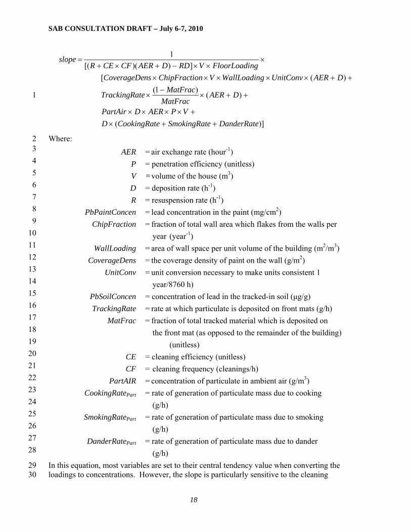
In addition to this regression equation, a mechanistic mass-balance model was developed. This model accounts for the three dominant sources of lead to indoor dust: penetration of ambient air into the indoor environment, tracking of lead soil into the building, and flaking of lead-containing paint from walls. Removal occurs due to ventilation and routine cleaning. The model preserves the total mass in the system and accounts for the accumulation of both lead and particulate on the floor and in the indoor air. The particulate must be included in the model in order to calculate the lead dust concentration because the denominator of the concentration is total dust mass. Thus, in addition to the lead sources, there is also an indoor source of mass from cooking, smoking, and human dander that contributes to dust but is not expected to contain appreciable concentrations of lead. By converting the mass-balance differential equations to difference equations, the model can be integrated forward in time. For the hazard standard calculation, however, the dust levels are expected to be relatively constant in time and not to be subject to any short-term perturbations, such as renovation activities. Thus, the model equations can be solved directly for the steady-state solutions. These solutions provide total dust mass and total lead mass, and from these both the loading and concentration can be calculated. Thus, the steady-state solutions can be used to derive the slope in the equation:
LoadingSlope
Concen ×=1 38
39 This slope is then given by (also derived as equation 3 in Appendix A):
17
SAB CONSULTATION DRAFT – July 6-7, 2010
)](
)()1()([
]))([(1
DanderRateeSmokingRateCookingRatDVPAERDPartAir
DAERMatFrac
MatFracteTrackingRa
DAERUnitConvgWallLoadinVonChipFractinsCoverageDengFloorLoadiVRDDAERCFCER
slope
++×+××××
++×−
×
++×××××
×××−+×+
=
1
2 3 4 5 6 7 8 9
10 11 12 13 14 15 16 17 18 19 20 21 22 23 24 25 26 27 28
29 30
Where:
AER = air exchange rate (hour-1) P = penetration efficiency (unitless) V = volume of the house (m3) D = deposition rate (h-1) R = resuspension rate (h-1) PbPaintConcen = lead concentration in the paint (mg/cm2) ChipFraction = fraction of total wall area which flakes from the walls per
year (year-1) WallLoading = area of wall space per unit volume of the building (m2/m3) CoverageDens = the coverage density of paint on the wall (g/m2) UnitConv = unit conversion necessary to make units consistent 1
year/8760 h) PbSoilConcen = concentration of lead in the tracked-in soil (μg/g) TrackingRate = rate at which particulate is deposited on front mats (g/h) MatFrac = fraction of total tracked material which is deposited on
the front mat (as opposed to the remainder of the building) (unitless)
CE = cleaning efficiency (unitless) CF = cleaning frequency (cleanings/h) PartAIR = concentration of particulate in ambient air (g/m3) CookingRatePart = rate of generation of particulate mass due to cooking
(g/h) SmokingRatePart = rate of generation of particulate mass due to smoking
(g/h) DanderRatePart = rate of generation of particulate mass due to dander
(g/h) In this equation, most variables are set to their central tendency value when converting the loadings to concentrations. However, the slope is particularly sensitive to the cleaning
18

SAB CONSULTATION DRAFT – July 6-7, 2010
1 2 3 4 5
6 7 8 9
10 11 12 13 14 15 16 17 18 19
20 21 22 23 24 25 26 27 28 29 30 31 32 33 34 35 36
38 39 40 41 42 43 44
frequency, building volume, and outdoor soil tracking rate, and distributions are available in the literature for each of these variables. Thus, for each hypothetical person in the Monte Carlo simulation, each of these three variables will be sampled using a pseudo-random number and the resulting slope will be calculated. Then the hazard standard will be converted from a loading to a concentration using the combination of inputs for that person.
At present, the mechanistic model only describes the floor loading-to-concentration relationship and does not model the accumulation of lead and dust on window sills. The processes governing such accumulation are not as well understood. The model could be extended, however, so that a separate slope could be developed for the window sill conversion.
Each of these two alternative conversion methods has strengths and limitations. The regression equation is based on a nationally-representative dataset with sufficient samples across different housing vintages, outdoor soil concentrations, and indoor paint concentrations. The regression equation has highest reliability for the range of loadings and concentrations in the original dataset, and the hazard standard is expected to fall within that range. The equation is specific to residences, however, and it cannot be easily extended to public and commercial buildings. In addition, the regression equation does not allow any incorporation of variability due to the difference in physical attributes and cleaning patterns among buildings. The underlying data show a wide spread across the loading-concentration parameter space, indicating wide house-to-house variability (see Appendix A).
The mechanistic model, on the other hand, allows for extension of the model to public and commercial buildings, provided the physical processes are described adequately and the proper input values can be developed. Because public and commercial buildings tend to be larger, more people come in and out of the buildings daily (thus introducing more dander to the indoor environment and diluting the indoor dust) and the cleaning patterns are different. Thus, these buildings can be expected to have a very different loading-to-concentration relationship from houses. The model, however, assumes that the indoor environment is well-mixed and contains no concentration gradients; thus, it can be applied to any portion of the public or commercial building where this assumption is valid. The mechanistic model also allows for the loading-to-concentration conversion to incorporate house-to-house variability. The model is subject to uncertainty, however, because of the relatively simple form of the physical equations and the absence of information about some of the variable inputs. The model has been calibrated against the HUD dataset and then compared to one additional dataset (see Appendix A), and is expected to return reasonable estimates for the national population in the range of the hazard standard. There currently are no data supporting relationships, however, between window sill loadings and concentrations and unless such slopes are developed, the same slopes as those used for the floor dust would have to be used in developing the window sill hazard standard.
3.4. Characterizing Exposure Variables 37
3.4.1. Human activity patterns
For the purposes of this approach, an exposure profile describes the amount of time spent by a simulated individual from the population of interest in various microenvironments during a one-year period. The time spent in various microenvironments is provided as an input to subsequent components of the conceptual model presented here to determine the uptake of lead and associated health impacts. A collection of profiles represents a random sample drawn from the target population and it is intended that the statistical properties of the collection of profiles
19

SAB CONSULTATION DRAFT – July 6-7, 2010
approximate the statistical properties of the target population (in this case, U.S. children under age 6 and all U.S. adults). The simulated individuals spend varying amounts of time in different microenvironments, each with different distributions of lead concentrations, and this approach allows for the characterization of the resulting differences in lead uptake and the associated health impacts.
1 2 3 4 5
6
7 8 9
10 11 12 13
14 15 16 17 18
19
20 21 22 23 24 25 26 27 28 29 30 31 32 33 34 35 36 37
38
3.4.1.1. Populations of interest
Children under age 6 were selected as a target population for developing commercial and public building hazard standards because they are the population considered most susceptible to adverse health effects from exposure to lead-containing dust in residences. This choice is consistent with studies performed by EPA in support of the RRP rule for residential buildings (USEPA 2008c). In order to capture the variability in time spent in commercial and public buildings by children of various ages under age 6, this population is further divided into six, one-year age groups (0-1, 1-2, etc.) for the purposes of estimating exposure concentrations (see Section 3.5).
In addition to children under age 6, the approach for commercial and public buildings includes consideration of adverse health effects in adults. As a result, U.S. adults were also selected as a target population. To accommodate variations in exposures with changes in the amount of time spent in various microenvironments as adults age, this population will be further divided into age groups based on expected changes in activity patterns with age.
3.4.1.2. Developing exposure profiles
Exposure profiles will be developed using data from CHAD (USEPA 2009b) for the target population and algorithms from the APEX model. Developed by the EPA’s National Exposure Research Laboratory, CHAD contains data collected from several studies designed to capture human activity patterns, and consists of one or more diaries of activities of each participant during the 24-hour period. It is commonly used in exposure assessment and provides required inputs to several EPA exposure models, such as HAPEM, SHEDS, and APEX1. Some applications of CHAD data in exposure assessments by EPA include the characterization of inhalation exposures in EPA’s National Air Toxics Assessment (NATA) and numerous reviews of the National Ambient Air Quality Standards (NAAQS) for criteria pollutants. Among the various datasets available in CHAD, only the National Human Activity Pattern Study (NHAPS) dataset contains data from a nationally-representative sample. This study, sponsored by the EPA and conducted by the University of Maryland, contains responses from 9,386 participants collected between October 1992 and September 1994. Because it is deemed that NHAPS data may not be sufficient to generate large enough sample of exposure profiles, other studies will also be included to develop activity patterns of simulated individuals. These other studies contain data that is collected from the following specific geographic locations: Cincinnati, Ohio; Baltimore, Maryland; California children study; California adults and youth study; Denver, Colorado; Los Angeles, California; Valdez, Alaska; and Washington, DC.
1 HAPEM = Hazardous Air Pollutant Exposure Model; SHEDS = Stochastic Human Exposure and Dose Simulation Model; APEX = Air Pollutants Exposure Model.
20

SAB CONSULTATION DRAFT – July 6-7, 2010
1 2 3 4 5 6 7 8 9
10 11
12 13 14 15 16 17 18 19 20 21 22 23 24 25 26 27 28 29
30 31 32 33 34 35 36 37 38 39 40 41 42
43 44
To generate the activity pattern of a simulated individual for a one-year period, one needs to develop a composite diary of one year from individual 24-hour diaries. A simple approach is to assume that the individual engages in same set of activities and spends same amount of time for an entire period characterized by a CHAD diary. For example, a randomly sampled weekday diary from CHAD data can be assumed to be applicable for all weekdays for a simulated individual. While this approach may capture between-person variability in activity patterns in the target populations, the variation in day-to-day activities of the simulated individual is not modeled. Consequently this approach may result in unrealistically large or small exposure times. Therefore, a probabilistic algorithm that can also capture day-to-day variation in the activity patterns of simulated individuals needs to be applied to develop composite diaries from individual 24-hour diaries.
The Air Pollution Exposure Model (APEX) is a peer-reviewed EPA model that is used to assess inhalation exposure for criteria and toxic air pollutants. The APEX model currently incorporates two stochastic methods to develop composite diaries to evaluate inhalation exposure. The diversity-autocorrelation algorithm assembles multi-day diaries based on reproducing realistic variability in a user-selected key diary variable – the variable that is assumed to have dominant influence on exposure. This algorithm works by first creating diary pools from the CHAD data. A diary pool is a group of CHAD diaries that has a common diary variable that has significant effect on activity patterns. For example, diary pools can be created for each day type (weekday, weekend day) and season (summer, non-summer) because it is expected that the activities of a target population significantly differ from weekday to weekend and between a summer day and a non-summer day. Once diary pools are created, each diary in the pool is assigned a rank, or “x-score,” based on the key activity variable. The composite diary is then assembled based on the x-scores using the longitudinal diary assembly algorithm. This algorithm aims to reproduce the user-supplied statistics D and A. The D statistic quantifies the relative importance of within-person and between-person variances in the key activity variable. The A statistic quantifies the day-to-day autocorrelation, which characterizes the similarity in diaries from day to day. Additional details of this algorithm are presented in the APEX technical support document (USEPA 2008d).
The second algorithm, the Cluster-Markov algorithm, also stochastically generates composite diaries from individual 24-hour period diaries. This approach was developed to better represent variability in activity patterns among simulated individuals. This algorithm first groups the CHAD diaries into two or three groups of similar patterns for each of the 30 combinations of day type (summer-weekday, non-summer weekday and weekend), demographic group (males and females), and age group (0-4, 5-11, 12-17, 18-64, 65+). Next, for each combination of day type and demographic group, category-to-category transition probabilities are defined by the relative frequencies of each second-day category associated with each given first-day category where the same individual was observed for two consecutive days. A composite diary of one year is constructed by first randomly selecting one daily activity pattern from each of the CHAD categories to represent that particular day type and demographic group. Finally, a sequence of daily activities for a one-year period is generated as a one-stage Markov chain process using the category-to-category transition probabilities.
To generate a sufficiently large number of profiles (on the order of a tens of thousands), this approach will apply both of the above algorithms and evaluate them for their statistical
21

SAB CONSULTATION DRAFT – July 6-7, 2010
properties. The algorithm that most adequately represents both the within-person and between-person variability will ultimately be applied to characterize the human activity patterns.
1 2
3
4 5 6 7 8
9 10 11 12 13
14 15 16 17 18 19 20 21 22 23
3.4.1.3. Defining microenvironments of interest
Children under age 6 While the time spent by children under age 6 in commercial and public buildings is of primary interest, their time spent in other microenvironments also contributes to overall lead uptake and therefore must be well characterized. In this approach, time spent by children under age 6 in the following microenvironments is estimated from CHAD data:
• Residences; • Child-occupied facilities (COF); • Outdoors; • Traveling; and • Public and commercial buildings.
It is assumed that the time spent in public and commercial buildings includes any time spent in an indoor building environment that is not a residential building or child-occupied facility, and is estimated from CHAD data by aggregating several location categories. The average, median, and 95th percentile of times spent in these microenvironments from CHAD data for the six children’s ages considered are presented in Table 3-2. Note that the CHAD data contain over 100 location descriptions. For this approach, these locations were aggregated into the five categories mentioned above. For example, the time spent traveling includes general travel, motorized travel, travel by walking, and waiting for bus, train, or other vehicle. Similarly, time spent in other building includes time spent in public buildings (e.g., libraries, museums), hospitals, and commercial buildings (e.g., grocery stores, restaurants)2.
2 This uses the CHAD terminology for “public” and “commercial”, as distinct from this proposal’s terminology, thereby breaking out “hospitals”.
22

SAB CONSULTATION DRAFT – July 6-7, 2010
1
Table 3-2 Children’s Time Spent in Selected Microenvironments, by Age
Age Residence COF Outdoor Travel Public/Commercial Buildings
Average time spent (Hours)
0 - 1 21.32 0.45 0.51 0.81 0.81
1 - 2 20.81 0.53 1.00 0.82 0.76
2 - 3 19.96 0.73 1.4 0.95 0.84
3 - 4 19.56 1.01 1.44 0.96 0.94
4 - 5 18.96 1.38 1.66 0.92 0.99
5 - 6 18.15 2.17 1.73 1.03 0.84
Median time spent (Hours)
0 - 1 22.00 0 0 0.67 0
1 - 2 21.42 0 0.42 0.58 0
2 - 3 20.50 0 0.67 0.67 0
3 - 4 20.00 0 0.83 0.75 0
4 - 5 19.25 0 1.00 0.75 0
5 - 6 18.17 0 1.00 0.75 0
95th percentile of time spent (Hours)
0 - 1 24.00 2.71 2.50 2.42 3.91
1 - 2 24.00 6.16 3.84 2.66 3.50
2 - 3 24.00 7.83 5.25 2.83 3.41
3 - 4 24.00 8.34 5.00 2.92 4.00
4 - 5 24.00 8.75 5.68 2.41 3.96
5 - 6 23.50 8.83 5.76 2.84 3.75
2
3 4 5 6 7
8 9
10 11
12 13 14 15
Adults
As with children under age 6, adults’ time spent in commercial and public buildings is of primary interest; however, their time spent in other microenvironments also contributes to overall lead uptake and therefore must be well characterized. In this approach, time spent by adults in the following microenvironments is estimated from CHAD data:
• Residences; • Outdoors; • Traveling; and • Public and commercial buildings.
It is assumed that the time spent in public and commercial buildings includes any time spent in an indoor building environment that is not a residential building, and is estimated from CHAD data by aggregating several location categories. The average, median, and 95th percentile of times spent in these microenvironments are presented in Table 3-3. These data are presented for
23

SAB CONSULTATION DRAFT – July 6-7, 2010
1 2
3
adults in five different age groups, which were developed by grouping ages with similar activity patterns.
Table 3-3. Adults’ Time Spent in Selected Microenvironments, by Age Group
Age Home Outdoor Travel Public/Commercial
Buildings Average time spent (Hours)
18 - 24 15.84 1.46 1.6 5.07
24 - 30 15.62 1.3 1.58 5.45
30 - 40 16.01 1.41 1.59 4.94
40 - 60 16.26 1.39 1.58 4.73
60 + 19.71 1.21 1.06 1.99
Median time spent (Hours)
18 - 24 15.22 0.3 1.2 5
24 - 30 14.7 0.17 1.17 5.33
30 - 40 15.08 0.27 1.18 4.18
40 - 60 15.5 0.25 1.08 3.67
60 + 20.5 0.17 0.58 0.92
95th percentile of time spent (Hours)
18 - 24 23.25 7.585 4.103 11.25
24 - 30 23.381 7.613 4.381 12.25
30 - 40 23.633 7.24 4.36 11.5
40 - 60 23.75 7 4.667 11.417
60 + 24 6.25 3.592 8.418
4
5
6 7 8 9
10 11 12 13 14 15 16 17 18
3.4.2. Other exposure variables Exposure variables other than the time spent in each microenvironment also affect the overall exposure of a child or adult to lead. These characteristics or variables include the ingestion rate of dust and soil, the intake rate of lead in the diet, the intake rate of lead in water, the ventilation rate, the lead inhalation and ingestion absorption rates, and the maternal blood lead when the child is born. In order to account for inter-individual variability in exposure in the target populations, those exposure variables expected to have the highest sensitivity and to vary the most strongly will be sampled from distributions. These include the ingestion of soil and dust by age group, background water lead intake, and background diet lead intake. Distributions for the ingestion of soil and dust will be generated from information in the Child-Specific Exposure Factors Handbook (USEPA 2008b) and the Exposure Factors Handbook (USEPA 1997). To estimate the distributions of lead dietary and water intake, the LifeLine Model (The LifeLine Group 2008) will be used to estimate a distribution of intakes across the population by age (for children under age 6) and age group (for adults). The ventilation rate and maternal blood lead
24

SAB CONSULTATION DRAFT – July 6-7, 2010
1 2 3 4 5 6 7 8 9
10 11 12 13 14 15
17 18 19 20 21
will not be sampled, but central tendency estimates will be taken in order to conserve computational resources; inhalation exposures are not anticipated to contribute in large measure to total lead exposure compared to soil and dust ingestion (USEPA, 2006) and the ventilation rate is not anticipated to be a sensitive variable. In addition, given the elimination rate of lead in children, maternal blood lead has only a minor impact on a child’s blood lead levels beyond the age of six months with subsequent blood lead levels determined primarily by environmental exposures. For the absorption fractions, these variables may be sensitive in describing the child’s overall response to lead exposure, but information in the literature is currently insufficient to derive distributions, so central tendency values will be used.
The sampled values for each variable differ across the different ages (for children under age 6) and age groups (for adults). To account for the potential correlations across ages, these variables will be sampled from age-specific distributions to ensure the same percentiles are used for each age/age group. For example, if a child has 90th percentile ingestion of soil and dust at age 1, they will also have 90th percentile ingestion of dust at age 5, and the actual ingestion values will be taken from the separate distributions for each age.
3.5. Estimating Exposure Concentrations 16 For each hypothetical person, the Monte Carlo sampling provides dust, soil, and air lead concentrations for each relevant microenvironment. The concentrations in each microenvironment must then be combined to provide overall air, soil, and dust concentrations for input into the blood lead model. First, the floor and window sill dust concentrations in each microenvironment are combined according to the equation:
22
23 24 25 26 27 28 29 30 31 32
33 34 35 36 37
tsilltfloor fracsillfracfloordust ,, ×+×=
where:
dust = the average dust exposure concentration in that microenvironment
floor = the concentration of lead in dust on the floor fracfloor,t = fraction of dust exposure arising from floor dust for age
range t sill = the concentration of lead in dust on the window sill fracsill,t = fraction of dust exposure arising from sill dust for age
range t The fracfloor,t variable will be adjusted for each age/age range to account for expected differences between infants, toddlers, preschoolers, kindergartners, and adults. Then, the concentrations for air, soil, and dust across microenvironments will be combined using the fraction of the time spent in each microenvironment for the specific age/age group. The following equation will be used:
25

SAB CONSULTATION DRAFT – July 6-7, 2010
∑
∑
=
=
×= n
iti
n
iiti
t
f
concenfconcen
1,
1,
exp,
)( 1
2 3 4 5 6 7 8
9 10 11 12 13 14 15 16 17
where:
concenexp,t = the exposure concentration for age range t fi,t = fraction of time spent in each microenvironment for age
range t conceni = the concentration in each microenvironment n = the number of microenvironments in which exposure to
the media occurs In the case of air concentrations, the person is assumed to be exposed to air concentrations in all microenvironments. The person is assumed only to be exposed to dust, however, when indoors (either in the home or outside the home) but not when outdoors or in a vehicle. Similarly, the soil concentrations are only combined using the fractions of time in an outdoor microenvironment. A separate blood lead model input variable accounts for the total ingestion of dust and soil mass and the fraction of total dust+soil ingestion that arises from soil. Thus, provided that the dust and soil concentrations represent the average concentrations to which the person is expected to be exposed as a result of their activity pattern, the approach assumptions are compatible with the blood lead modeling assumptions.
26

SAB CONSULTATION DRAFT – July 6-7, 2010
4. Estimation of Blood Lead Levels 1
4.1. Children under age 6 2
4.1.1. Overview of blood lead models for children 3 4 5 6 7 8 9
10 11 12 13
14 15 16 17 18 19 20 21 22 23 24 25
26 27 28 29 30 31 32 33
34 35 36 37 38 39 40 41
42 43
A number of different approaches are available to estimate children’s blood lead levels in response to defined exposure scenarios (USEPA 2006). Approaches that have been implemented include explicit pharmacokinetic models (where the movement of lead is simulated through compartments with defined volumes and perfusion rates), biokinetic models (where lead moves from compartment to compartment based on first-order rate constants), and empirical models that predict blood lead as a simple regression-like function of steady-state exposure concentrations. In addition to these general-purpose models that take media concentrations or exposures as their inputs, there have been several studies (Rabinowitz et al. 1985, Lanphear 2007) where the impacts of residential renovation activities on blood lead levels have been estimated directly for specific populations of children.
Among the available models, EPA’s IEUBK model (USEPA 2010a) is by far the most thoroughly tested and frequently used for assessment of the impacts of exposures in air, soil, house dust, diet and water on children’s blood lead concentrations. The IEUBK model was originally developed by EPA’s Office of Air Quality Planning and Standards (OAQPS) to support analyses of air quality standards starting in 1985. The model implements a biokinetic model developed by Harley and Kneip (1985) that predicts blood lead levels in children 0-7 years old in response to specified lead exposures. In 1991, responsibility for further development of the IEUBK model was given to the Technical Review Workgroup (TRW), composed of representatives from several EPA program and regional offices. The model was released to the public in 1991 and has been updated continuously since then without basic changes to the model structure, although recommended default exposure factor and environmental concentration values have changed as new data have become available.
The EPA All Ages Lead Model (AALM), now under development, aims to extend beyond IEUBK capabilities to model external Pb exposure impacts (including over many years) on internal Pb distribution not only in young children, but also in older children, adolescents, young adults, and other adults well into older years (up to 90 years of age) (USEPA 2005). The AALM essentially uses adaptations of the IEUBK exposure module features, coupled with adaptations of IEUBK biokinetics components (for young children) and of the Leggett model’s biokinetics components (for older children and adults). The AALM has not yet undergone sufficient development and validation for it to be recommended for general risk assessment use.
EPA’s Clean Air Science Advisory Committee (CASAC) reviewed the use of the IEUBK in support of the 1990 revisions to the National Ambient Air Quality Standard (NAAQS) for lead, and the structure and parameter values in the model have also been reviewed by the Indoor Air Quality and Total Exposure Committee of the Science Advisory Board (SAB). The IEUBK has been subject to external peer review, its performance has been tested against a number of large data sets, and its predictions have been compared to competing pharmacokinetic and biokinetic models (NIEHS 1998, USEPA 2006). The IEUBK was the primary blood lead assessment model used in EPA’s risk assessment supporting the lead NAAQS revision (USEPA 2007).
The most plausible alternatives to the IEUBK include the “Leggett” biokinetic model (Leggett 1993) and the pharmacodynamic model developed by O’Flaherty et al. (1993, 1995). The
27

SAB CONSULTATION DRAFT – July 6-7, 2010
1 2 3 4 5 6 7 8 9
10 11 12 13 14 15
16 17 18 19 20 21 22 23 24
25 26 27 28 29 30 31 32 33 34 35 36
37
38 39 40 41 42 43 44 45
Leggett model was developed with support from the International Agency for Radiological Protection (ICRP) to support risk assessment for radionuclides of lead and related elements. The model is technically sophisticated, simulating the transfer of lead among 15 compartments in the body, based on a large body of age-specific biokinetic data on lead and other metals. In addition, the default time step for biokinetic simulation is one day instead of the minimum one-month time step used in the IEUBK model, which suggests that the Leggett model might be better suited to modeling the impacts of short-term exposures. Despite these potential advantages, the Leggett model has not undergone the same degree of testing against environmental data sets as has the IEUBK. In addition, the Leggett model does not include a detailed exposure model like the IEUBK;and pathway-specific daily intakes must be specified by the user. Detailed comparisons of the IEUBK and Leggett model results indicate that, for plausible exposure scenarios and absorption fraction values, the Leggett model tends to predict higher children’s lead uptake and blood lead levels than the IEUBK for similar exposures (USEPA 2006). One important feature of the Leggett model not shared by the IEUBK is that it has the capability to model blood lead overall from birth through adulthood.
The O’Flaherty pharmacodynamic model (O’Flaherty et al. 1993, 1995) is likewise more complex and technically sophisticated in some ways than the IEUBK model. As noted above, it is a truly pharmacodynamic model with lead transfer modeled between compartments with defined age-specific volumes and perfusion rates. In addition, the O’Flaherty model explicitly models the age-related changes in bone growth and deposition/depuration processes. Like the Leggett model, however, the O’Flaherty et al. model has not been subject to the same degree of calibration and testing against human data sets (particularly children) as has the IEUBK. As will be discussed below, in comparison studies, the O’Flaherty et al. and Leggett models tend to give similar blood lead predictions for defined adult exposure scenarios.
Empirical (regression-type) blood lead models based on environmental concentrations were not considered for use in this analysis because the available models (Lanphear et al. 1998b, Schwartz et al. 1998, USEPA 1998) predict steady-state blood lead levels in adults or children assumed to be facing constant exposures from soil, dust, and paint. They are thus poorly suited to estimating the impacts of variable exposures arising from renovation activities. Two studies were also identified (Rabinowitz et al. 1985, Lanphear et al. 2007) that directly estimated the potential impacts of residential renovation on children’s blood lead levels. While these studies provide helpful support for the current analysis, neither is suited for exposure-response analysis since the number of exposed subjects is small in both studies and both were conducted in older urban neighborhoods where renovation hazards may not be typical of those in the rest of the U.S. The study by Rabito et al. (2007) was likewise limited to estimating the blood lead impacts of demolition activities in a high-lead area.
4.1.2. IEUBK
Based on the evaluation described above, the IEUBK was selected for modeling blood lead concentrations for children under 6 years of age in the residential exposure scenario. The IEUBK model is a multicompartmental pharmacokinetics model that, in the default mode, provides estimates of long-term (annual average) blood lead levels in children (birth to 7 years). Used in batch mode, the IEUBK model can provide estimates of blood lead concentrations over shorter time intervals; run in batch mode, temporal resolution of one month can be achieved. That is, input variables can be specified and blood lead outputs can be obtained for each month of exposure. The exposure module simulates intake of lead for six exposure media: air, diet
28

SAB CONSULTATION DRAFT – July 6-7, 2010
1 2 3 4 5 6 7 8 9
10 11 12
13 14 15 16 17 18
19 20 21 22 23 24 25 26 27 28 29 30 31
33 34 35 36 37 38 39 40 41 42 43 44
(excluding drinking water), drinking water, outdoor soil/dust, indoor dust, and other. Input variables, including absorption fraction and inhalation rate, water intake, dietary intakes of specific food classes, and outdoor soil/dust and indoor dust ingestion rates, are user-specified. Age-specific lead inhalation uptakes are estimated for exposure to outdoor and indoor air, based on age-dependent estimates of time spent indoors and outdoors, estimates of indoor and outdoor air lead concentrations, and age-dependent inhalation rates. Additionally, a respiratory tract adsorption fraction is used to account for both deposition of inhaled lead in the respiratory tract and absorption of deposited lead from either the respiratory tract or from the gastrointestinal (GI) tract. The model also contains an option for calculating indoor dust lead concentrations based on an empirical relationship among air, outdoor soil/dust, and indoor dust lead levels. Ingestion uptake is calculated using absorption fractions that are specific to the ingested medium (diet, drinking water, outdoor soil/dust, or indoor dust).
Under the default option, total gastrointestinal (GI) lead uptake is modeled as being composed of a saturable and an unsaturable component using the IEUBK default parameters describing the relative importance of these two components as a function of total lead intake. The user may change the model inputs describing the saturable pathway, or turn it off completely. The outputs of the uptake module are estimates of the masses of lead absorbed into the body over time as a function of concentrations in the various exposure media.
In the biokinetic module of the IEUBK model, absorbed lead (from ingestion and inhalation) is assumed to appear immediately in the plasma-extracellular fluid (ECF) compartment. The plasma-ECF compartment constitutes the central compartment in the biokinetic model from which exchange to all other compartments occurs. Trabecular and cortical bone (which are not directly coupled in the IEUBK model) constitute the main long-term storage compartments, with the estimated turnover in other compartments being more rapid. The binding capacity of the red blood cell (RBC) compartment is modeled as being saturable, simulating the limited capacity of aminolevulinate dehydratase (ALAD) and other lead-binding proteins. Lead excretion occurs through a urine pathway (distinct from the kidney compartment). Hepatobiliary secretion is coupled with the liver compartment, with a minor component of excretion from “other soft tissues” (i.e., skin, hair, and nails). The sole output from the IEUBK model is blood lead concentrations for each exposure period; the model does not support the estimation of bone accumulation.
4.2. Adults 32
4.2.1. Overview of blood lead models for adults The relative merits of the various models for predicting blood lead levels were discussed in Section 4.1. As noted there, the AALM has not yet undergone sufficient development or validation for it to be recommended for use in this approach. To the extent that the performance of the most well-documented adult blood lead models has been compared, the Leggett biokinetic model (Leggett 1993) and the O’Flaherty et al. (1993, 1995) pharmacokinetic model produce generally similar results for simple exposure scenarios. Both models, despite their differences in structure, include relatively sophisticated representations of lead transport in the body and both are capable of modeling short- and long-term exposures. The Leggett model has been chosen as the primary method for adult blood lead modeling in this approach for several reasons. First, development of the Leggett model built on a very large database of animal and human data relating to the behavior of lead and other metals in the body. In contrast, the O’Flaherty et al.
29

SAB CONSULTATION DRAFT – July 6-7, 2010
1 2 3 4 5 6 7 8
9 10 11 12 13 14 15 16 17 18 19 20 21 22 23 24 25 26 27 28
29 30 31 32
model is based primarily on animal (rodent) data, and its adaptation to predicting human blood lead levels relies heavily on allometric scaling. While the IEUBK has been subjected to much more testing and calibration than either the Leggett or O’Flaherty et al. models, among models that are capable of predicting adult blood lead, the Leggett model likewise has been much more thoroughly tested than the O’Flaherty et al. model. One important additional consideration is that, as part of previous analyses, OAQPS and OPPT have adapted the Leggett model for easy batch mode operation, which greatly facilitates the analyses of large numbers of exposure scenarios and sensitivity analyses of important variables.
4.2.2. Leggett model The Leggett model is capable of predicting changes in blood lead levels for exposed individuals over their entire lifespan (birth to 90 years old). The compartmental structure of the Leggett model was patterned after similar models developed by the ICRP to model the age-specific biokinetics of calcium-like radionuclides (Leggett 1993). In the biokinetic component of the Leggett model, the movement of absorbed lead (from ingestion and inhalation) through various body “compartments” is simulated. The model is “biokinetic,” rather than “pharmacokinetic,” because transfers between compartments are controlled by first-order transfer coefficients (equivalent to first-order rate constants), rather than being perfusion controlled. The values for the transfer rates were estimated using a range of values from adult human radioactive tracer studies, autopsy data from adults and children, and data from animal studies related to the absorption, deposition, and excretion of lead and chemically similar elements (Leggett 1993). Leggett developed estimates of biokinetic parameters for six age categories: newborn (0 to 100 days), 1 year, 5 years, 10 years, 15 years, and 25 years and older, with age-specific transfer parameters for children estimated by interpolation between the nearest values. Transfer factors for children were adjusted to take into account the more rapid bone turnover (calcium/lead addition and resorption) in children compared with adults. The Leggett model does not accept exposure concentrations directly. Instead, it accepts total inhalation and ingestion intakes (administered doses) as inputs. Thus, the exposure concentration time series are converted to intakes using specified input values, as described in Table 6-3.
There are several options for defining the adult exposure period when modeling lead exposures associated with different hazard standards. For this approach, blood lead levels will be modeled starting at age 18 through age 80, with initial blood lead levels sampled from the distribution of blood lead levels for 18-year-olds from the most recent NHANES database.
30

SAB CONSULTATION DRAFT – July 6-7, 2010
1
31

SAB CONSULTATION DRAFT – July 6-7, 2010
5. Application of the Model for Estimating Hazard Standards 1
2 3 4 5 6 7 8 9
10 11 12 13 14 15 16
17 18 19
20 21 22 23
24 25 26 27 28 29
31 32 33 34 35 36 37 38 39
40
41
42
Sections 2 through 4 describe the methods used for calculating a person’s blood lead concentration distribution by specifying lead dust loadings for the dust and window sill candidate hazard standards and simulating numerous hypothetical individuals, each with different sampled behaviors and environmental media concentrations. The purpose of this model, however, is to calculate the floor and window sill dust lead loadings corresponding to the target blood lead levels, or solving for the input of the model with a known output. This section explains the methodology used for calculating dust lead loadings for the candidate hazard standards which result in a target blood lead level.
As described in Section 3, media concentrations and some exposure variables will be sampled probabilistically for all microenvironments except for the candidate commercial/public buildings hazard standards (floor and window sill) for each realization. Therefore, each realization will result in a different blood lead concentration, as each sampling will likely have unique set of media concentrations. The same distributions will be used for thousands of unique realizations to generate a distribution of blood lead concentrations associated with each set of candidate hazard standards.
Because the relationship between hazard standards and the various contributions to blood lead concentration does not exist as an equation in closed form, selecting a set of candidate hazard standards that result in a target blood lead concentration consists of two steps:
1. Create a response surface to correlate candidate dust and window sill lead dust loading levels with blood lead levels. The response surface will be constructed by running many iterations with different target loading levels, with a limited number of realizations for each iteration, to generate rough approximations of the corresponding blood lead levels.
2. Using this response surface, predict the target loading that corresponds to a prespecified point on the blood lead concentration distribution, and run the model to confirm/deny this prediction. Repeat iteratively until the loading value corresponding with the prespecified point has been precisely determined. This step will involve running fewer iterations with a much higher number of realizations, thus creating highly precise relationships between target loadings and blood-lead levels.
5.1. Creating the Target Loading-to-Blood-Lead Response Surface 30 Because multiple distributions are sampled for each realization, the resulting distributions of blood lead levels may have a wide range. Therefore, many realizations may need to be simulated in order for the blood lead distribution to become stable (i.e., adequately represent the underlying inputs). To minimize the number of iterations required to identify the candidate hazard standards corresponding to the prespecified blood lead concentration distribution point, a response surface will be created for a range of candidate hazard standards that will provide an educated guess as to what loading will correspond to a particular target blood lead percentile. Because the response surface will be used only to provide a preliminary estimate of final candidate loadings, fewer realizations can be conducted with each iteration to reduce calculation time.
32

SAB CONSULTATION DRAFT – July 6-7, 2010
5.2. Estimating the Candidate Hazard Standard Using the Response Surface 1 After generating a response surface for range of candidate loadings, a rough estimate of the relationship between candidate loadings and blood lead levels will be known. Using this relationship, a set of candidate loadings can be estimated to correspond with a target blood lead level, and the model is run to determine if the target blood lead level is reached with sufficient precision. Because this analysis is composed of a large number of sampled distributions (Table 5-1), it is suspected that thousands of realizations will be required to reach a stable blood lead level distribution. Stability of the distribution will be assessed using statistical methods roughly comparing variability of the distribution to its median with variability measures generated by such techniques as the boot-strap method
2 3 4 5 6 7 8 9
10
11
c.
Table 5-1. Key Input Variables or Variable Groups Sampled in the Public and Commercial Buildings Model
Group
Sampling independent
or correlated? Variable or Variable Groupa Sampling Notes Dust lead loading, floor, commercial/public building Fixed with each iteration Candidate hazard
standards Correlated Dust lead loading, sill, commercial/public building Fixed with each iteration
Exposure location Independent Time spent in each environment Sampled, resampled annually Independent Ingestion of lead in drinking water Sampled, resampled annually Independent Ingestion of lead in diet Sampled, resampled annually Independent Daily ingestion of dust and soil Fixed, changes annually Independent Ventilation rate Fixed, changes annually
Exposure
Independent Lung absorption efficiency Fixed Dust lead loading, floor, all other areas Sampled, once per realization
Correlated Dust lead loading, sill, all other areas Sampled, once per realization
Independent Soil lead concentration, outdoors Sampled, once per realization
Independent Air lead concentration, indoors Sampled, once per realization
Lead loadings/ concentrations in environmental media
Independent Air lead concentration, outdoors Sampled, once per realization a Variables mentioned above may represent multiple distributions, and therefore the number of sampled distributions will actually be greater than what is presented above. In addition, if additional or better input data are found, additional variables mentioned above may be sampled as well.
12
14 15 16 17
5.3. Sensitivity Analysis 13
To better understand each variable’s impact on the candidate hazard standards identified, a sensitivity analysis will be conducted on each variable. This sensitivity analysis will provide a better understanding of which variables are most influential to the model, and therefore which variables are most influential in determining the candidate hazard levels. This analysis will use
c The simulations will be run until the standard error of the 90th percentile value of the output blood lead distribution is estimated to be less than 10 per cent of its median.
33

SAB CONSULTATION DRAFT – July 6-7, 2010
1 2
3 4 5 6
7 8 9
10 11 12
methods consistent with considerations in the Agency intended to conform to current best practice.
All sensitivity analyses will be conducted in deterministic mode. Deterministic mode is defined using a single value for each variable (i.e., no sampling will occur). In deterministic mode, each unique group of input variables will have one unique output value. Because no sampling will occur, results will not be impacted by the convergence of output distributions.
Elasticity will be used to determine the impact of each input variable. Elasticity is defined as the percent change in a model output value (i.e., blood-lead level) that results from a fixed percent change in a model input variable value with all other variable values held to a constant baseline value. Baseline case is defined as the central tendency values for all variables in the model. By modifying each variable by the same percent change, elasticicity can be compared across variables to better understand to which variables the model is most/least sensitive.
0
01
0
01
xxx
yyy
Elasticity−
−
= 13
14
15
16
17
18
19 20 21 22 23 24 25
26 27 28 29 30 31 32
33 34 35 36
where:
y1 = blood lead level, sensitivity case
yo = blood lead level, baseline case
x1 = property value, sensitivity case
xo = model input property value, baseline case
An elasticity of 1 means that a percent change in an input value is linearly related to a percent change in the output value. An elasticity of 0 means that changing the input value has no effect on the output value. A elasticity in absolute value less than 1 occurs when a percent change in an input value results in a greater percent change in an output value. An elasticity of | <1 | occurs when a percent change in an input value results in a smaller percent change in an output value. A negative value for elasticity indicates that the output value varies in the opposite direction to the input value change.
For all characteristics (sampled or fixed), variability in a property can be nonlinear. To address this in the sensitivity analysis, two analyses will be conducted: a local analysis (representing small changes in a variable) and a global analysis (for larger changes). For the local analysis, each variable in the model will be varied by ± 5% from the central tendency; for the global analysis, each variable will be varied by ± 50% from the central tendency. If the elasticity of a variable is different between the local and global analysis, this indicates that this variable has a nonlinear relationship to blood lead.
Because the model will sample media concentrations from known distributions, additional information is known about the range of possible values from these distributions. Therefore, the sensitivity score will be calculated for variables which are sampled from a distribution. The sensitivity score is calculated by:
34

SAB CONSULTATION DRAFT – July 6-7, 2010
x
xElasticityScoreySensitivitμσ
* = 1
2
3
4
Where:
σx = standard deviation/geometric standard deviation of input distribution
µx = mean/geometric mean of input distribution
35

SAB CONSULTATION DRAFT – July 6-7, 2010
6. Data Needs 1
2 3
4 5 6 7 8 9
10
11 12 13
14 15 16
17 18 19 20 21 22 23
24 25 26 27 28 29 30 31
32 33 34 35 36 37 38
The quality of the results generated using the approach described in this document relies heavily on reliable input data. Among the most important data needs are:
• Media concentrations for residences; • Media concentrations for public and commercial buildings; • Media concentrations for near-roadway areas; • Media concentrations for outdoors; • Relationship between window sill and floor dust lead exposures; • Inputs to the blood lead models; and • Inputs to the mechanistic dust lead loading-to-concentration model.
This section discusses the data identified thus far for each of the types of data, with the exception of the inputs to the mechanistic loading-to-concentration model and those for the floor-dust-to-sill-dust correlation, which are discussed in Appendix A.
6.1.1. Media concentrations for residences As shown in Table 3-1, the distribution of indoor dust floor loadings, indoor dust window sill loadings, and indoor air lead concentrations are needed in residences.
For the floor and window sill loadings, the HUD survey of lead-based paint in homes (USEPA 1995) will be used. This survey provides data on wipe and vacuum samples of floor and window sill loadings in 312 homes. Distributions will be developed from these loadings to capture the distribution of lead loadings in the housing stock. The wipe sample loadings will be used in favor of the vacuum samples because they are expected to provide a better estimate of the total lead loading. The survey provides weighting factors used to update the data to the 1997 housing stock, and the weights will be incorporated when developing the distributions.
For the air distributions, the approach proposes to use the Air Quality System (AQS) monitoring system to develop suitable distributions (USEPA 2010b). In the system, each monitor is assigned a monitoring objective code, as shown in Table 6-1. In order to capture the typical exposure concentrations for the national population, data from all monitors with coverage in 2009 and 2010 for the codes 6 (Population Exposure) and G (General/Background) will be pulled. The data will be annually-averaged, and a distribution across the available values will be developed. In order to capture the total lead content, the analysis will focus on lead Total Suspended Particulate (TSP) monitors.
These monitors provide outdoor air concentrations around the country. To generate the indoor concentrations, a factor will be applied to the outdoor concentrations to approximate the indoor concentration. Thatcher and Layton (1995) report that Colome et al. (1992) found an average indoor/outdoor ratio of 0.7 in 35 California homes. This is also the average indoor/outdoor ratio predicted by the approach’s mechanistic dust model when applied to the HUD data set (see Appendix A), suggesting the ratio is plausibly applied in this approach. Thus, the ambient concentration will be multiplied by 0.7 to convert to an approximate indoor concentration.
36

SAB CONSULTATION DRAFT – July 6-7, 2010
Table 6-1. AQS Monitor Objective Codes Monitor
Code Monitor Objective 0 UNKNOWN 1 UPWIND BACKGROUND 2 MAX PRECURSOR EMISSIONS IMPACT 3 MAX OZONE CONCENTRATION 4 EXTREME DOWNWIND 5 OTHER 6 POPULATION EXPOSURE 7 SOURCE ORIENTED 8 REGIONAL TRANSPORT 9 WELFARE RELATED IMPACTS G GENERAL/BACKGROUND H HIGHEST CONCENTRATION I INVALID CODE TEST
1
2
3 4 5 6
7 8 9
10 11
12 13 14 15 16
17 18 19 20
21 22 23
6.1.2. Media concentrations for public and commercial buildings As shown in Table 3-1, the distribution of indoor air lead concentrations are needed in public and commercial buildings to develop the lead hazard standards. The dust concentrations will be the target hazard standards and will not be approximated from literature data.
Data may not be available to separately define residential and public and commercial building ambient air concentrations. Thus, the approach will likely use the same ambient concentration as used in residences. An extensive literature search will be conducted to identify typical indoor/outdoor air concentration ratios in public and commercial buildings for use in converting to indoor concentrations.
6.1.3. Media concentrations near roadways An exposure concentration in air is also required for the “traveling” microenvironment. Attempts will be made to locate air lead concentrations which are typical on and near roadways. Then, the assumption will be made that the “traveling” microenvironment concentration equals the outdoor ambient concentration.
6.1.4. Media concentrations outdoors
For the outdoor microenvironment, the approach requires outdoor soil concentrations. The HUD survey (USEPA 1995) provides soil concentrations at residences. These concentrations will be used to develop residential soil distributions.
For outdoor locations away from the home, available public and commercial soil lead concentrations will be compared to the residential values and a separate distribution will be developed if needed.
37

SAB CONSULTATION DRAFT – July 6-7, 2010
1
2 3 4 5 6
7 8 9
10 11 12 13 14 15
16 17 18 19 20 21 22 23 24 25 26
27
28
6.1.5. The relationship between window sill and floor exposures In order to combine the indoor dust concentrations into a single exposure level for model input, the floor and sill levels must be combined according to the approximate relative ingestion of each. The LRRP rule (USEPA 2008a) used a weighting strategy based on the surface area. This would give approximately 1% weighting to sills and 99% weighting to floors.
A literature search was conducted to determine if any other exposure assessments have made assumptions of the relative contributions of floor and sill. To date, only a single document has been found. The assessment focused on lead and arsenic exposures associated with the presence of indoor paint. It was submitted to the ATSDR and was prepared by the California Department of Health Services (CDC 2002). In the assessment, the assumption was made that sills contribute 1% in infants, 5% in toddlers, 17% in young children, 25% in older children, and 25% in adults. These values appear to represent the authors’ professional judgment and do not reflect any measurements that could inform the weighting strategy chosen for this approach. Consequently, the relative floor area assumption will be used.
In addition to combining the floor and sill concentrations into a single aggregate dust concentration, the candidate window sill hazard standard will need to be determined corresponding to each candidate floor hazard standard. Because these two loadings are expected to be correlated in a single building, the approach proposes to develop an empirical relationship to combine them in residences. One potential dataset is the HUD survey data (USEPA 1998). The data from homes constructed before 1980 were used to develop a preliminary relationship between floors and sills for this approach. Figure 6-1 shows the regression model for this dataset; details of this analysis are described in Appendix A. The data were natural-log-transformed, since doing so resulted in an apparently higher regression coefficient. The correlation between the variables indicates some correlation (r=0.43). The equation relating the two loadings would then be
91.056.4 FloorSill ×=
Figure 6-1. Regression Relationship between Ln(Sill) and Ln(Floor) for the HUD Data
y = 0.9067x + 1.5167R2 = 0.1864
-6
-4
-2
0
2
4
6
8
10
12
-2 -1 0 1 2 3 4 5 6 7
ln(floor loading in μg/ft2)
ln(s
ill lo
adin
g in
μg/
ft2 )
29
38

SAB CONSULTATION DRAFT – July 6-7, 2010
1 2 3 4 5
6 7 8 9
10 11 12 13 14 15 16 17
In addition, the Rochester data (Lanphear et al., 1998a) could be used to derive an empirical relationship. As in the HUD data, the natural-log-transformed variables are better correlated than the untransformed variables; the regression is presented in Figure 6-2. In this case, the correlation appears slightly higher (r=0.48) and the equation relating sill to floor loading would be
80.01.22 FloorSill ×= A literature search will be conducted to determine if additional details about the empirical relationship can be found. Both of these empirical relationships are more applicable to residences than to public and commercial buildings. However, to date, no data have been found which could relate window sill and floor loadings in public and commercial buildings. The approach proposes to use the residential relationships, although this assumption will introduce uncertainty into the hazard standard estimates.
Figure 6-2. Regression Relationship between Ln(Sill) and Ln(Floor) for the Rochester
Data
y = 0.7976x + 3.0953R2 = 0.2348
0
2
4
6
8
10
12
14
0 1 2 3 4 5 6 7 8 9 10
ln(floor loading in μg/ft2)
ln(s
ill lo
adin
g in
μg/
ft2 )
18 19 20 21 22 23 24 25 26
27 28 29
6.1.6. Inputs to the blood lead models
The blood lead models require a number of inputs in addition to the air, soil, and dust concentrations. Table 6-2 shows the inputs and the proposed values for each of these inputs. As a starting point, the selected values are the same as those used in the development of the benefits analysis for the lead renovation and repair rule (USEPA 2008c). Several input values were then updated with data from recently published literature. Other values, however, were found to still reflect the best information available. These included the lead absorption fractions and the fraction of ingested soil+dust which is soil.
In 2008, EPA published a new edition of its Child-Specific Exposure Factors Handbook, in which updated values for total indoor/outdoor dust ingestion and ventilation rate were presented (USEPA 2008b). Where ages were expressed as a range in that report, rates for intermediate
39

SAB CONS
40
ULTATION DRAFT – July 6-7, 2010
1 2 3 4 5 6 7 8
9 10 11 12 13
14 15 16 17
For the dietary and water lead intakes, distributions will be generated using the LifeLine TM Model (The LifeLine Group 2008). This model will predict distributions of water and dietary lead intake for each medium by age group. Because the IEUBK includes both a water consumption term and a water concentration term, the consumption will be set to one liter per day and the intake will be used in place of the concentration.
ages were interpolated using linear trendlines. Mean and 95th percentile values are available for both the dust ingestion and the ventilation rates. For the dust ingestion, the mean and and 95th percentile values will be used to establish a lognormal distribution which will then be sampled as part of the Monte Carlo simulation. For ventilation rates, the mean age-specific values will be used in developing the hazard standards. Because inhalation rates have been found in previous analyses not strongly to affect the predicted blood lead levels in children (USEPA 2006), this variable is not sampled in order to minimize the number of Monte Carlo realizations necessary to resolve the blood lead distribution.
The IEUBK value for maternal blood lead level has been updated using data from the most recent NHANES survey. These data from 2007 and 2008 (CDC 2009b) reveal that the nationally weighted GM blood lead level among women aged 18 through 45 has fallen over the last fifteen years to 0.847 μg/dL.

SAB CONSULTATION DRAFT – July 6-7, 2010
Table 6-2. Proposed Blood Lead Model Input Values Variable Value
IEUBK Default Age Ranges (Years)
Group Variable Variable Name
0.5
to 1
1 to
2
2 to
3
3 to
4
4 to
5
5 to
6
6 to
7
Basis/Derivation
Daily ventilation rate (cubic
meters [m3]/day) Ventilation rate 5.4 (95%
8.1) 8.0 (95%
12.8) 9.5 (95%
15.9) 10.9 (95%
16.2) 10.9 (95%
16.2) 10.9 (95%
16.2) 12.4 (95%
18.7)
EPA Child-Specific Exposure Factors
Handbook (USEPA 2008b) with interpolation
for intermediate ages
Absolute inhalation absorption
fraction (unitless)
• Lung absorption (IEUBK)
• Absolute respiratory absorption fraction
(Leggett)
0.42 USEPA (1989) Appendix A
Indoor air Pb concentration
Indoor air Pb concentration (percentage of
outdoor)
100%
Inha
latio
n
Time spent outdoors
Time spend outdoors (hours/day) Not used
These values are taken directly into account when developing the
exposure concentrations
Water consumption
(L/day)
Water consumption (L/day) 1 1 1 1 1 1 1
These values are set to 1, since the water
consumption will be incorporated into the
water ingestion estimate used in the next row.
Water Pb concentration
(µg/L)
Pb concentration in drinking water (µg/L) Distribution to be estimated from the LifeLine model
The LifeLine TM model will be used to estimate the distribution of lead
intake from water. Because the water
consumption is set to 1 in the model, the intakes can be entered in place
of the lead concentrations.
Drin
king
Wat
er In
gest
ion
Absolute absorption
• Total percent accessible (IEUBK)
• Absolute GI
50 % (Single value used across all age ranges)
Assumed similar to dietary absorption (see
"Total percent
41

SAB CONSULTATION DRAFT – July 6-7, 2010
Table 6-2. Proposed Blood Lead Model Input Values Variable Value
IEUBK Default Age Ranges (Years)
Group Variable Variable Name
0.5
to 1
1 to
2
2 to
3
3 to
4
4 to
5
5 to
6
Basis/Derivation
6 to
7
(unitless) absorption fraction (Leggett)
accessible" under Diet below).
Dietary Pb intake (µg/day)
Dietary Pb intake (µg/day)
Distribution to be
estimated from the LifeLine model
Distribution to be
estimated from the LifeLine model
Distribution to be
estimated from the LifeLine model
Distribution to be
estimated from the LifeLine model
Distribution to be
estimated from the LifeLine model
Distribution to be
estimated from the LifeLine model
Distribution to be
estimated from the LifeLine model
The LifeLine TM model will be used to estimate the distribution of dietary
intake by age group
Die
t
Absolute absorption (unitless)
(1)Total percent accessible (IEUBK)
(2) Absolute GI absorption fraction
50%
Alexander et al. (1974) and Ziegler et al. (1978)
as cited in USEPA (2006, section 4.2.1)
Out
door
Soi
l/Dus
t and
Indo
or D
ust I
nges
tion
Outdoor soil/dust and indoor dust weighting factor
(unitless)
• Outdoor soil/dust and indoor dust
ingestion weighting factor (percent
outdoor soil/dust) (IEUBK)
• Outdoor soil/dust and indoor dust ingestion rates
calculated separately using same proportion
of outdoor soil/dust ingestion (Leggett)
45 percent
This is the percent of total ingestion that is
outdoor soil/dust. Value reflects best judgment
and consideration (results published by van Wijnen et al. (1990), as cited in (USEPA, 1989).
The van Wijnen et al. study examined at tracer studies of ingestion rates for rainy days and non–
rainy days. It was assumed that rainy days were associated with all
outdoor soil/dust ingestion and non-rainy days were associated with a combination of outdoor soil/dust and
indoor dust with the delta representing outdoor
soil/dust.
42

ULTATION DRAFT – July 6-7, 2010
Table 6-2. Proposed Blood Lead Model Input Values Variable Value
IEUBK Default Age Ranges (Years)
Group Variable Variable Name
0.5
to 1
1 to
2
2 to
3
3 to
4
4 to
5
5 to
6
6 to
7
Basis/Derivation
SAB CONS
43
Total indoor dust + outdoor soil/dust ingestion (mg/day)
Amount of outdoor soil/dust and indoor dust ingested daily
(mg)
Distribution estimated
from percentiles
Distribution estimated
from percentiles
Distribution estimated
from percentiles
Distribution estimated
from percentiles
Distribution estimated
from percentiles
Distribution estimated
from percentiles
Distribution estimated
from percentiles
Distribution estimated from the EPA Child-Specific Exposure Factors Handbook (USEPA 2008b),
excluding cases of soil-pica and geophagy
Absolute gastrointestinal
absorption (outdoor
soil/dust and indoor dust)
(unitless)
• Total percent accessible (IEUBK)
• Absolute GI absorption fraction
(Leggett)
0.30 for both outdoor soil/dust and indoor dust
(USEPA, 1989) reflects evidence that Pb in
indoor dust and outdoor soil/dust is as accessible
as dietary Pb and that indoor dust and outdoor soil/dust ingestion may
occur away from mealtimes (resulting in enhanced absorption relative to exposure during meal events).
Oth
er
Maternal PbB (μg/dL)
Maternal PbB concentration at childbirth, μg/dL
0.847
NHANES 2007-2008, national weighted GM of all women aged 18-45
(CDC 2009b)

SAB CONSULTATION DRAFT – July 6-7, 2010
44

SAB CONSULTATION DRAFT – July 6-7, 2010
7. References 1
2 3
4 5
6 7 8
9 10 11
12 13
14 15
16 17 18
19 20 21 22
23 24
25 26
27 28 29
30 31 32
33 34 35 36
37 38 39
Alexander, F. W.; Clayton, B. E.; Delves, H. T. (1974) Mineral and Trace-Metal Balances in Children Receiving Normal and Synthetic Diets. Q. J. Med. 43: 89-111.
Bellinger, D. (2008) Very low lead exposures and children’s neurodevelopment. Curr. Opp. Pedriatr. 20(2):172-7.
Canfield, R. L.; Henderson, C. R., Jr.; Cory-Slechta, D. A.; Cox, C.; Jusko, T. A.; Lanphear, B. P. (2003) Intellectual impairment in children with blood lead concentrations below 10 μg per deciliter. N. Engl. J. Med. 348: 1517-1526.
Centers for Disease Control and Prevention (CDC). (2002) Review of Dust Sampling Data for the 45th Street Artists’ Cooperative. Available online at: http://www.atsdr.cdc.gov/HAC/pha/PHA.asp?docid=81&pg=0.
Centers for Disease Control and Prevention (CDC). (2005). Third National Report on Human Exposure to Environmental Chemicals. Atlanta (GA): CDC. http://www.cdc.gov/exposurereport/
Centers for Disease Control and Prevention (CDC). (2009a). Fourth National Report on Human Exposure to Environmental Chemicals. Atlanta (GA): CDC. http://www.cdc.gov/exposurereport/
Centers for Disease Control and Prevention (CDC). (2009b) National Health and Nutrition Examination Survey (NHANES), 2007-2008. Available online at: http://www.cdc.gov/nchs/nhanes/nhanes2007-2008/nhanes07_08.htm
Chaney, RL, Sterrett, SB, and Mielke, HW (1984) The potential for heavy metal exposure from urban gardens and soils, pp. 37-84. In: J.R. Preer ed. Proceedings of the symposium on heavy metals in urban gardens. Agricultural Experiment Station, University of the District of Columbia, Washington. Available at: http://indytilth.org/Links/Chaney_Exposure.pdf
Chen A; Cai B; Dietrich K; Radcliffe J; Rogan W. (2007). Lead exposure, IQ, and behavior in urban 5-to 7-year-olds: does lead affect behavior only by lowering IQ? Pediatrics 119: e650.
Chiodo L; Jacobson, S; Jacobson, L. (2004). Neurodevelopmental effects of postnatal lead exposure at very low levels. Neurotoxicology and Teratology 26: 359-371.
Colome, S.D.; Kado, N. Y.; Jaques, P; and Kleinman, M. (1992). Indoor-outdoor air pollution relations: particulate matter less than 10 µm in aerodynamic diameter (PM10) in the homes of asthmatics. Atmospheric Environment 26A, 2173-2178.
Harley, N and Kneip, T. (1985). An Integrated Metabolic Model for Lead in Humans of All Ages. Final Report to the U.S. EPA, Contract No, B33899 with NYU School of Medicine, Dept. of Environmental Medicine, January 30, 1985.
Holmgren, GSS, Meyer, MW, Chaney, RL and Daniels, RB (1993) Cadmium, Lead, Zinc, Copper, and Nickel in Agricultural Soils of the United States of America. J. Environ. Qual. 22:335-348. Available at: http://espm.berkeley.edu/classes/espm-120/Website/Holmgren1993.pdf
Jusko T; Henderson Jr C; Lanphear B; Cory-Slechta D; Parsons P; Canfield R. (2008). Blood lead concentrations< 10 g/dL and child intelligence at 6 years of age. Environmental Health Perspectives 116: 243.
45

SAB CONSULTATION DRAFT – July 6-7, 2010
1 2
3 4 5 6 7
8 9
10 11 12
13 14 15
16 17
18
Lanphear, B.P.; Burgoon, D.A.; Rust, S.W., Eberly, S; and Galke, W (1998a). Environmental exposures to lead and children’s blood lead levels. Environmental Research, 76 (2): 120-130.
Lanphear, B.P., Matte, T.D., Rogers, J., Clickner, R.P., Dietz, B., Bornschein, R.L., Succop, P., Mahaffey, K.R., Dixon, S., Galke, W., Rabinowitz, M., Farfel, M., Rohde, C., Schwartz, J., Ashley, P., Jacobs, D.E. (1998b) The contribution of lead-contaminated house dust and residential soil to children’s blood lead levels. A pooled analysis of 12 epidemiologic studies. Environ. Res. 79(1): 51-68.
Lanphear, B.P.; Hornung, R.; Khoury, J.; Yolton, K.; Baghurst, P.; Bellinger, D.C.; Canfield, R.L.; Dietrich, K.N.; Bornschein, R.; Greene, T.; Rothenberg, S.J.; Needleman, H.L.; Schnaas, L.; Wasserman, G.; Graziano, J.; and Roberts, R. 2005. Low-level environmental lead exposure and children's intellectual function: an international pooled analysis. Environmental Health Perspectives. 113: 894-899.
Lanphear, B.P. et al. 2007. Comments on “An Approach for Estimating Changes in Children’s IQ from Lead Dust Generated during Renovation, Repair and Painting,” “CASAC Tables,” and the PowerPoint™ presentation at the July 9 -10 CASAC review meeting.
Leggett, R.W. 1993. An Age-Specific Kinetic Model of Lead Metabolism in Humans. Environmental Health Perspectives. 101: 598-616.
The LifeLine Group, 2008. The LifeLine model, v5. http://www.thelifelinegroup.org/lifeline/index.htm 19
20 21 22
23 24 25 26
27 28 29
30 31 32
33 34 35 36
37 38
39 40 41
Massachusetts Department of Environmental Protection (MADEP). (2002) Background Levels of Polycyclic Aromatic Hydrocarbons and Metals in Soil; Technical Update. Available at: http://www.mass.gov/dep/cleanup/laws/backtu.doc
Mielke, HW, Anderson, JC, Berry, KJ, Mielke, PW, Chaney, RL and Leech, M (1983) Lead concentrations in inner-city soils as a factor in the child lead problem. Am. J. Public Health 73:1366-1369. Available at: http://www.ncbi.nlm.nih.gov/pmc/articles/PMC1651267/pdf/amjph00647-0022.pdf
Miranda M; Kim D; Galeano M; Paul C; Hull A; Morgan S. (2007). The relationship between early childhood blood lead levels and performance on end-of-grade tests. Environmental Health Perspectives 115: 1242.
Nash, D., Magder, L., Lustberg, M., Sherwin, RW., Rubin, RJ., Kauffman, RB., Silbergeld, EK. (2003) Blood Lead, Blood Pressure, and Hypertension in Perimenopausal and Postmenopausal Women. JAMA. 289(12):1523-1532.
National Institute of Environmental Health Sciences (NIEHS). (1998.) Proceedings of a Workshop on Model Validation and Concepts and Their Application to Lead Models. Env. Health Pers. Volume 106, Supplement 6 (1998) http://ehp.niehs.nih.gov/docs/1998/Suppl-6/toc.html
Navas-Acien et al. (2007). Lead Exposure and Cardiovascular Disease—A Systematic Review. Env. Health Pers. 115(3):472-482.
Nawrot TS, Thijs L, Den Hond EM, Roels HA, Staessen JA. (2002). An epidemiological re-appraisal of the association between blood pressure and blood lead: a meta-analysis. J Hum Hypertens 16:123–131.
46
SAB CONSULTATION DRAFT – July 6-7, 2010
1 2 3
4 5 6 7
8 9
10 11
12 13 14
15 16
17 18 19
20 21 22
23 24
25 26 27
28 29 30
31 32 33 34
35 36
37 38 39
Nigg J; Knottnerus G; Martel M; Nikolas M; Cavanagh K; Karmaus W; Rappley M. (2008). Low blood lead levels associated with clinically diagnosed attention-deficit/hyperactivity disorder and mediated by weak cognitive control. Biological Psychiatry 63: 325-331.
Nigg J; Nikolas M; Knottnerus G; Cavanagh K; Friderici K. (2010). Confirmation and extension of association of blood lead with attention-deficit/hyperactivity disorder (ADHD) and ADHD symptom domains at population-typical exposure levels. Journal of Child Psychology and Psychiatry, and Allied Disciplines 51: 58-65.
O'Flaherty, E. J. (1993) Physiologically based models for bone-seeking elements. IV. Kinetics of lead disposition in humans. Toxicol. Appl. Pharmacol. 118: 16-29.
O'Flaherty, E. J. (1995) Physiologically based models for bone-seeking elements: V. Lead absorption and disposition in childhood. Toxicol. Appl. Pharmacol. 131: 297-308.
Ohio Environmental Protection Agency (EPA). (2008) Closure Plan Review Guidance for RCRA Facilities; Appendix B: Development of Alternate Metal Standards. Available at: http://web.epa.ohio.gov/dhwm/old_cprg/AppendixB_AlternateMetalStandards.pdf
Rabinowitz, M., Leviton, A., and Bellinger, D. 1985. Home Refinishing, Lead Paint, and Infant Blood Lead Levels. Amer. J. Pub. Health. 75(4): 403-404
Rabito, F; Iqbal, S; Shorter, C; Osman, P; Phillips, P; Langlois, E; White, L. (2007). The association between demolition activity and children’s blood lead levels. Environmental Research 103: 345-351.
Roy, A; Bellinger, D; Hu, H; Schwartz, J; Wright, R; Palaniappan, K; Balakrishnan, K. (2008). Lead associated deficits in executive function and behavior in 3-7 year old children in Chennai, India. Epidemiology 19: S306.
Schwartz, J. (1994). Low-level lead exposure and children's IQ: a meta-analysis and search for a threshold. Environ Res 65(1):42-5.
Schwartz, J., Ashley, P., and Jacobs D.E. (1998). The contribution of lead-contaminated house dust and residential soil to children's blood lead levels. A pooled analysis of 12 epidemiologic studies. Environ Res 79(1):51-68.
Scinicariello, F., Yesupriya, A., Chang, M-H, Fowler, BA., (2010). Modification by ALAD of the Association between Blood Lead and Blood Pressure in the U.S. Population: Results from the Third National Health and Nutrition Examination Survey. Env. Health. Pers. 118(2):159-264.
Shacklette, HT and Boerngen, JG (1984) Element concentrations in soils and other surficial materials of the conterminous United States: U.S. Geological Survey Professional Paper 1270, 105 p. Available at: http://pubs.usgs.gov/pp/1270/pdf/PP1270_508.pdf; http://pubs.usgs.gov/pp/p1648/p1648.pdf
Succop, P, Clark,S, Tseng,C-Y, Bornschein, R and Chen, M (2001) Evaluation of Public Housing Risk Assessment Data. Environmental Geochemistry and Health 23: 1-15.
Surkan P; Zhang A; Trachtenberg F; Daniel D; McKinlay S; Bellinger D. (2007). Neuropsychological function in children with blood lead levels< 10 [mu] g/dL. Neurotoxicology 28: 1170-1177.
47

SAB CONSULTATION DRAFT – July 6-7, 2010
1 2 3 4
5 6
7 8 9
10 11 12 13
14 15 16
17 18 19 20
21 22 23
24 25 26 27
28 29 30 31
32 33 34 35
36 37
38 39 40
Téllez-Rojo, M. M.; Bellinger, D. C.; Arroyo-Quiroz, C.; Lamadrid-Figueroa, H.; Mercado-García, A.; Schnaas-Arrieta, L.; Wright, R. O.; Hernández-Avila, M.; Hu, H. (2006) Longitudinal associations between blood lead concentrations < 10 μg/dL and neurobehavioral development in environmentally-exposed children in Mexico City. Pediatrics 118: e323-e330.
Thatcher, T. L.and Layton, D. W. (1995) Deposition, Resuspension, and Penetration of Particles Within a Residence. Atmospheric Environment. 29(13): 1487-1497.
U.S. Environmental Protection Agency (USEPA). (1989) Review of National Ambient Air Quality Standard for Lead: Exposure Analysis Methodology and Validation. EPA-450/2-89-011. Research Triangle Park, NC: Office of Air Quality Planning and Standards; June.
U.S. Environmental Protection Agency (USEPA). (1995) Report on the National Survey of Lead-Based Paint in Housing: Appendix C1: Characterizing Baseline Environmental Lead Levels in the Nation’s Housing Stock. EPA 747-R95-004. Office of Pollution Prevention and Toxics.
U.S. Environmental Protection Agency (USEPA). (1997). Exposure Factors Handbook (Final Report). EPA/600/P-95/002F a-c. Washington, DC: Office of Research and Development; September.
U.S. Environmental Protection Agency (USEPA). 1998. Risk Analysis to Support Standards for Lead in Paint, Dust, and Soil. Office of Pollution Prevention and Toxics. EPA 747-R-97-006. Appendix G: Health Effects Associated with Exposure to Lead and Internal Lead Doses in Humans http://www.epa.gov/lead/pubs/403risk.htm
U.S. Environmental Protection Agency (USEPA). (2005) All ages lead model [draft version 1.05]. Research Triangle Park, NC: National Center for Environmental Assessment. Available at: http://cfpub.epa.gov/ncea/cfm/recordisplay.cfm?deid=139314.
U.S. Environmental Protection Agency (USEPA). (2006) Air Quality Criteria for Lead, Volume I of II. Research Triangle Park, NC: National Center for Environmental Assessment – RTP Office. EPA/600/R-5/144aF. October. Available at: http://cfpub.epa.gov/ncea/cfm/recordisplay.cfm?deid=158823
U.S. Environmental Protection Agency (USEPA). (2007). Lead: Human Exposure and Health Risk Assessments for Selected Case Studies Volume I. Human Exposure and Health Risk Assessments - Full-scale. EPA-452/R-07-014a. http://www.epa.gov/ttn/naaqs/standards/pb/s_pb_cr_td.html
U.S. Environmental Protection Agency (USEPA) Activity-Related Communication. (2007). Email Correspondence between Elizabeth Margosches of U.S. EPA and Richard Hornung of Cincinnati Children's Hospital Medical Center. Title of email: re: coefficients of a piecewise linear model. July 20, 2007.
U.S. Environmental Protection Agency (USEPA). (2008a). Lead; Renovation, Repair, and Painting Program; Final Rule. Federal register (73 FR 21692, April 22, 2008).
U.S. Environmental Protection Agency (USEPA). (2008b). Child-Specific Exposure Factors Handbook. EPA/600/R-06/096F. Washington, DC: Office of Research and Development; September.
48

SAB CONSULTATION DRAFT – July 6-7, 2010
1 2 3
4 5 6 7
8 9
10 11
12 13
14 15
16 17
18 19 20
21 22 23
24 25 26
27 28
U.S. Environmental Protection Agency (USEPA). (2008c). Economic Analysis for the TSCA Lead Renovation, Repair, and Painting Program Final Rule for Target Housing and Child-Occupied Facilities Office of Pollution Prevention and Toxics (OPPT).
U.S. Environmental Protection Agency (USEPA). (2008d). Total Risk Integrated Methodology (TRIM) Air Pollutants Exposure Model Documentation (TRIM. Expo/APEX, Version 4.3) Volume II: Technical Support Document. Available at: http://www.epa.gov/ttn/fera/data/apex/APEX_UsersGuide_Vol2_Oct08.pdf
U.S. Environmental Protection Agency (USEPA). (2009a). Sierra Club etc. Settlement. (August, 2009).
U.S. Environmental Protection Agency (USEPA). (2009b). Consolidated Human Activity Database (CHAD). http://www.epa.gov/chad/.
U.S. Environmental Protection Agency (USEPA). (2010a). IEUBKwin32 Lead Model Version 1.1 Build 11. http://www.epa.gov/superfund/health/contaminants/lead/products.htm#ieubk
U.S. Environmental Protection Agency (USEPA). (2010b) Air Quality System (AQS) Database. Available online at: http://www.epa.gov/ttn/airs/airsaqs/aqsweb/aqswebwarning.htm.
van Wijnen J.H.; Clausing P.; Brunekreef, B. (1990) Estimated Soil Ingestion by Children. Environ Res. 51(2): 147-162.
Weaver, VM., Ellis, LR., Lee, B-K., Todd, AC., Shi, W., Ahn, K-D., Schwartz, B.S. (2008) Associations Between Patella Lead and Blood Pressure in Lead Workers. Amer. J. Ind. Med. 51:336–343
Westat, Inc. (2003) First National Environmental Health Survey of Child Care Centers; Final Report; Volume I. Prepared for the U.S. Department of Housing and Urban Development. July 15, 2003. Available at: http://www.nmic.org/nyccelp/documents/HUD_NEHSCCC.pdf
Wright, J; Dietrich, K; Ris, M.; Hornung, R; Wessel, S; Lanphear, B; Ho, M; Rae, M. (2008). Association of prenatal and childhood blood lead concentrations with criminal arrests in early adulthood. PLoS Med 5: e101.
Ziegler, E. E.; Edwards, B. B.; Jensen, R. L.; Mahaffey, K. R.; Fomon, S. J. (1978) Absorption and Retention of Lead by Infants. Pediatr. Res. 12: 29-34.
49

SAB CONSULTATION DRAFT – July 6-7, 2010
Appendix A. Loading to Concentration Conversion Methods
A-1

SAB CONSULTATION DRAFT – July 6-7, 2010
A-2

SAB CONSULTATION DRAFT – July 6-7, 2010
The indoor lead hazard standard prescribes the amount of lead allowed on the surface per unit area (lead loading). The blood lead models, however, cannot accept lead loadings as inputs. Instead, they require the lead concentration, or the amount of lead per mass of dust. Thus, as part of the derivation of the hazard standard, dust loadings must be converted to dust concentrations for input into the blood lead models. Two different estimates have been developed for this approach, based on two different methodologies: 1) a statistical regression model and 2) a mechanistic model. Sections A.1 through A.3 describe these estimates and highlight the strengths and limitations of each. Section A.4 describes the development of the regression used for the relationship between floor lead dust loading and window sill lead dust loading.
A.1 Development of a Regression Equation The National Survey of Lead-Based Paint in Housing ("HUD Survey Data") was used to develop a loading-to-concentration regression equation for this approach. The data, available in Appendix C-1 in a risk assessment (USEPA, 1998), provide information on wipe sample lead dust loadings, vacuum sample lead dust loadings, and blue nozzle lead concentrations on the floor for over 312 homes in different vintage categories: Pre1940, 1940-1959, 1960-1979, and Post1980. It is anticipated that the wipe samples better capture the total lead present in the home; the vacuum samples are subject to vacuum collection efficiencies. Thus, the wipe loadings were paired with the blue nozzle concentrations at each home to develop the loading-to-concentration statistical relationship. By doing so, the assumption is made that the concentration is roughly uniform across all particles and the particles collected by the blue nozzle device are representative of the true average concentration. In order to focus on the homes containing lead paint, only the data from the older three vintage categories were included. This eliminated 28 data points from the dataset. Some statistics from the reduced dataset are provided in Table A-1. In general, the spread in the data is large and covers loadings up to 375 μg/ft2 and concentrations up to 50,400 μg/g. The range of considered hazard standards is below the 95th percentile loadings, so the results of the regression are anticipated to apply to the hazard standard in residences.
Table A-1. Statistics from the HUD Survey Data
Loading (μg/ft2)
Concentration (μg/g)
Average 20.99 559.08 Min 0.51 0.09 Max 375.00 50400.00 5th percentile 1.25 33.85
25th percentile 3.27 101.75
50th percentile 7.43 201.00
75th percentile 17.38 374.25
95th percentile 96.10 1522.50
A-3

SAB CONSULTATION DRAFT – July 6-7, 2010
From the raw data, each loading and concentration was transformed by taking the natural log. Then, the regression was carried out using the untransformed variables and also the natural-log-transformed variables. Table A-2 shows the results of each regression.
Table A-2. Regression Analysis Results
Data Variable CoefficientStandard Error of
Coefficientt-stat p-value F-stat,
p-level Adjusted
R2
Intercept 159.74 195.86 0.82 0.42 Untransformed Slope 19.02 4.26 4.46 <0.0000
19.88, <0.0000 0.065
Intercept 3.93 0.10 38.11 <0.0000 Natural-log- transformed Slope 0.6655 0.42 15.71 <0.0000
246.75, <0.0000 0.465
The data are positively skewed, and the regression analysis reveals that the log-transformed data provide a regression with a larger adjusted R2 value. Thus, the log-transformed relationship is chosen, and after accounting for the natural log transformation, the equation relating concentration and loading is:
6553.096.50 LoadingConcen ×= .
Figure A-1 below shows the raw data and the regression relationship. The gray lines represent the 90th percentile in the loading and the concentration.
Figure A-1. HUD Data and the Regression Relationship
0
500
1000
1500
2000
0 20 40 60 80 100Loading (μg/ft2)
Con
cent
ratio
n ( μ
g/g)
HUD Data
Regression
A.2 Development of a Mechanistic Dust Model The mechanistic model is designed to capture the physical transfer of mass from one medium to another under the assumption of mass balance. Previous studies have also built mass balance models of indoor dust. Allott et al. (1994) constructed a mass balance model to estimate the
A-4

SAB CONSULTATION DRAFT – July 6-7, 2010
residence time of contaminated soil particles in the indoor environment based on observations in four homes in England contaminated by the Chernobyl incident. Thatcher and Layton (1995) constructed an indoor mass balance model of a home in California to estimate deposition rates, resuspension rates, and infiltration factors. Recognizing the key role of tracked-in soil on indoor dust loadings, Johnson (2008) built the DIRT model simulating the spatial pattern of tracked-in soil for a given total soil mass flux into the home. Layton and Beamer (2009) built a model simulating tracked-in soil and penetration of outdoor air and the subsequent physical processes governing indoor dust loadings. These models cannot be readily applied for developing an approach for the lead hazard standards, however, because they do not include any dust source from lead-containing paint. A new model was constructed for the hazard standard approach and the coefficients were optimized against all available data, as described below. Where applicable, the resulting coefficients are compared to those found in the above studies to help frame the model in the existing literature. This mechanistic model is deterministic in its underlying nature.
The general form of the mass balance equation for a single compartment of interest is:
Out Massof Flux In Massof Fluxdt
Massd−=
][
where:
d[Mass]/dt = change over time of the mass Flux of Mass In = flux of mass into the compartment Flux of Mass Out = flux of mass out of the compartment In the dust model, two “compartments” of interest are defined: the indoor air and the floor. Both of these compartments will contain particulates associated with indoor dust, and by parameterizing the processes that govern the flux of mass to and from each compartment, the model can provide an inventory of dust in the air and on the floor through time.
In the above equation, “mass” could refer to either the mass of lead that penetrates the home and settles on the floor in the dust or it could refer to the mass of the dust particles themselves. Because the blood lead model needs inputs of lead dust concentration, the mechanistic model must separately account for both the mass of lead and the mass of dust particulate that accumulates on the floor. Then, by dividing the total lead mass by the total dust mass, the model provides an estimate of the average lead dust concentration. Thus, for each compartment there are two separate equations, one for the lead mass and one for the dust particulate mass.
The dominant sources of lead to the indoor dust are ambient air particles which penetrate the indoor environment and settle on the floor, outdoor soil particles which are tracked into the home, and lead-containing paint which flakes or chips off the walls and settles to the floor. Dust particles have the same sources, although non-lead dust particles are also formed indoors through human activities such as cooking and smoking and by the accumulation of human and pet dander. Figure A-2 shows a schematic of the various lead and particulate mass flux terms used in the mechanistic model to account for all sources and sinks of mass.
A-5

SAB CONSULTATION DRAFT – July 6-7, 2010
Figure A-2. Mechanistic Indoor Dust Model Schematic
Outdoor Air Particles, Outdoor Air Pb in Particles
Settling
Outdoor Soil
Paint Particles, Pb in Paint
Deterioration
Tracking
Cleaning
Ceiling Height
Floor Area
Indoor Dust Particles, Indoor Pb in Dust
Resuspension
Penetration
Ventilation
Indoor Source of Non-Pb Particles
Indoor Air Particles, Indoor Pb in Particles
Settling
Outdoor Soil
Paint Particles, Pb in Paint
Deterioration
Tracking
Cleaning
Ceiling Height
Floor Area
Indoor Dust Particles, Indoor Pb in Dust
Resuspension
Penetration
Ventilation
Indoor Source of Non-Pb Particles
Indoor Air Particles, Indoor Pb in Particles
For the indoor air compartment, the fluxes for mass include penetration of air and particles from outdoors, ventilation of indoor air back to the outdoor environment, deposition of mass out of the air, resuspension of accumulated mass on the floor back into the air, generation due to indoor sources (where cooking and smoking are thought to dominate these sources), and generation due to the formation of human and pet danderd:
PbPbPb
PbPbPbPb
SourcesDanderSourcesIndoorFluxonResuspensi
FluxDepositionFluxnVentilatioFluxnPenetratiodt
dINAIR
++
+−−=
PartPartPart
PartPartPartPart
SourcesDanderSourcesIndoorFluxonResuspensi
FluxDepositionFluxnVentilatioFluxnPenetratiodt
dINAIR
++
+−−=
where:
d The presence of an HVAC system will tend to re-circulate indoor air, passing the air through a filter with each circulation. This system will tend to remove mass from the indoor environment (both in the air and on the floor) and act as a further sink. Because the circulation rate and filtration efficiency of such systems has not been comprehensively described in the literature and because use of such systems changes across the seasons and different geographic regions, removal of mass during recirculation is not included in the mechanistic model.
A-6

SAB CONSULTATION DRAFT – July 6-7, 2010
dINAIRPb/dt = change in time of the indoor air lead mass dINAIRPart/dt = change in time of the indoor air particulate mass Penetration Flux = penetration of air containing particles from outdoors Ventilation Flux = ventilation of indoor air back to the outdoor environment Deposition Flux = deposition of mass out of the air Resuspension Flux = resuspension of accumulated mass on the floor back into
the air Indoor Sources = generation of mass due to indoor sources such as cooking
or smoking Dander Sources = generation of mass due to human and pet dander In general, each flux is parameterized as either a constant source or as the mass of the "donor" compartment multiplied by the rate (expressed in reciprocal time) of the physical exchange process. In some cases, an efficiency factor is also included to account for any filtration of lead associated with the process. In addition, there is a separate flux term for the lead mass and for the particulate equations. For the Penetration Flux,
VPbAIRPAERFluxnPenetratio Pb ×××= VPartAIRPAERFluxnPenetratio Part ×××=
where:
Penetration FluxPb = penetration of air lead from outdoors (μg/h) Penetration FluxPart = penetration of air particles from outdoors (g/h) AER = air exchange rate (h-1) P = penetration efficiency (unitless) PbAIR = concentration of lead in ambient air (μg/m3) PartAIR = concentration of particles in ambient air (g/m3) V = volume of the house (m3) Because the air exchange rate (AER) specifies the number of times the indoor air is replaced by outdoor air in a given hour, it represents both the rate of penetration in and ventilation out. The ventilation flux out of the house is thus given by:
PbPb INAIRAERFluxnVentilatio ×=
PartPart INAIRAERFluxnVentilatio ×= where:
Ventilation FluxPb = ventilation of indoor lead in air back to the outdoor environment (μg/h)
Ventilation FluxPart = ventilation of indoor particulate in air back to the outdoor environment (g/h)
A-7

SAB CONSULTATION DRAFT – July 6-7, 2010
AER = air exchange rate (h-1) INAIRPb = indoor mass of lead in air (μg) INAIRPart = indoor mass of particulate in air (g) The deposition flux (Deposition Flux) is defined as the amount of mass in the air times a deposition rate:
PbPb INAIRDFluxDeposition ×=
PartPart INAIRDFluxDeposition ×=
where:
Deposition FluxPb = deposition of lead out of the air (μg/h) Deposition FluxPart = deposition of particulate out of the air (g/h) D = deposition rate (h-1) INAIRPb = indoor mass of lead in air (μg) INAIRPart = indoor mass of particulate in air (g) For resuspension, the amount of resuspended material depends on the total available mass on the floor multiplied by a resuspension rate:
PbPb FLOORRFluxonResuspensi ×=
PartPart FLOORRFluxonResuspensi ×=
where:
Resuspension FluxPb = resuspension of lead out of the air (μg/h) Resuspension FluxPart = deposition of particulate out of the air (g/h) R = deposition rate (h-1) FLOORPb = mass of lead on the floor (μg) FLOORPart = mass of particulate on the floor (g)
For the indoor sources of mass, each source is set equal to a constant rate:
0=PbcesIndoorSour
0=PbcesDanderSour
PartPartPart eSmokingRateCookingRatcesIndoorSour +=
PartPart DanderRatecesDanderSour =
A-8

SAB CONSULTATION DRAFT – July 6-7, 2010
where:
IndoorSourcesPb = source of lead due to cooking and smoking (μg/h); assumed to be zero.
DanderSourcesPb = source of lead due to formation of dander (μg/h); assumed to be zero.
IndoorSourcesPart = source of particulate due to cooking and smoking (g/h) CookingRatePart = rate of generation of particulate mass due to cooking
(g/h) SmokingRatePart = rate of generation of particulate mass due to smoking
(g/h) DanderSourcesPart = source of particulate due to formation of dander (g/h) DanderRatePart = rate of generation of particulate mass due to dander
(g/h).
So, using the penetration, ventilation, deposition fluxes, and indoor source terms, the equation for the change in time of the indoor air lead mass is:
PbPbPbPb FLOORRINAIRDINAIRAERVPbAIRPAER
dtdINAIR
×+×−×−×××=
PartPartPart
PartPartPartPart
DanderRateeSmokingRateCookingRat
FLOORRINAIRDINAIRAERVPartAIRPAERdt
dINAIR
++
+×+×−×−×××=
where:
dINAIRPb/dt = change in time of the indoor air lead mass (μg/h) dINAIRPart/dt = change in time of the indoor air particulate mass (g/h) INAIPRPb = indoor mass of lead in air (μg) INAIPRPart = indoor mass of particulate in air (μg) FLOORPb = mass of lead on the floor (μg) FLOORPart = mass of particulate on the floor (g) PbAIR = concentration of lead in ambient air (μg/m3) PartAIR = concentration of particulate in ambient air (g/m3) AER = air exchange rate (hour1) P = penetration efficiency (unitless) V = volume of the house (m3) D = deposition rate (h-1) R = resuspension rate (h-1)
A-9

SAB CONSULTATION DRAFT – July 6-7, 2010
CookingRatePart = rate of generation of particulate mass due to cooking (g/h)
SmokingRatePart = rate of generation of particulate mass due to smoking (g/h)
DanderRatePart = rate of generation of particulate mass due to dander (g/h).
For the indoor floor dust compartment (FLOOR), the fluxes include deposition of lead from the air onto the floor, resuspension of lead from the floor into the air, flaking of paint from the walls, tracking of lead from outdoor soil, and removal of lead due to routine cleaning:
1A)Equation(Pb
PbPbPbPbPb
FluxCleaning
uxTrackingFlFluxPaintFluxonResuspensiFluxDepositiondt
dFLOOR−++−=
1B)Equation(Part
PartPartPartPartPart
FluxCleaning
uxTrackingFlFluxPaintFluxonResuspensiFluxDepositiondt
dFLOOR−++−=
where:
dFLOOR/dt = change in time of the indoor floor mass Deposition Flux = deposition of mass out of the air onto the floor Resuspension Flux = resuspension of mass from the floor into the air Paint Flux = flaking of lead-containing paint onto the floor Tracking Flux = tracking of soil inside from outdoors Cleaning Flux = removal of lead due to routine cleaning. The deposition flux (Deposition Flux) and resuspension flux (ResuspensionFlux) retain the same form as in the INAIR equations. The paint flux is parameterized using a paint chipping fraction, a wall area expressed as the wall loading multiplied by the house volume, and lead paint concentration for the lead mass and the same paint chipping fraction and wall area with a coverage density for the particulate mass. The chipping fraction is explicitly assumed to account for the mass that falls on the floor rather than any mass that lands on window sills or other surfaces:
UnitConvgWallLoadinVonChipFracticenPbPaintConFluxPaint Pb ××××=UnitConvgWallLoadinVonChipFractinsCoverageDeFluxPaint Part ××××=
where:
PaintFluxPb = generation of lead in air due to deterioration of lead- containing paint (μg/h)
PaintFluxPart = generation of particulate in air due to deterioration of lead- containing paint (μg/h)
A-10

SAB CONSULTATION DRAFT – July 6-7, 2010
PbPaintConcen = lead concentration in the paint (mg/cm2) ChipFraction = fraction of total wall area which flakes from the walls per
year (year-1) V = volume of the home (m3) WallLoading = area of wall space per unit volume of the home (m2/m3) CoverageDens = the coverage density of paint on the wall (g/m2) UnitConv = unit conversion necessary to make units consistent (1
year/8760 h). The tracking flux (TrackingFlux) is parameterized specifically according to the limited data available about the process. Von Lindern et al. (2003) measured the amount of particulate deposited on front mats in 276 houses in two locations near the Bunker Hill Superfund Site. The lead levels reported in the paper are expected to be high-end and are not expected to represent general population exposures. This approach assumes, however, that the rate of accumulation of dust (as opposed to the lead in the dust) on doormats is not strongly affected by the location and can be used to represent a national population of homes. In addition, Thatcher and Layton (1995) measured the difference between particulate accumulation in tracked and untracked areas in the home as well as the amount on the front mat. From these two data sources, it is possible to estimate a distribution of mat particulate accumulation rates as well as the fraction of material that remains on the mat compared to being tracked into the home. For this reason, the tracking is parameterized as:
MatFrac
MatFracteTrackingRaenPbSoilConcFluxrackingT Pb)1( −
××=
MatFracMatFracteTrackingRaFluxrackingT Part
)1( −×=
where:
TrackingFluxPb = accumulation of tracked-in lead on the floor (μg/h) TrackingFluxPart = accumulation of tracked-in particulate on the floor (g/h) PbSoilConcen = concentration of lead in the tracked-in soil (μg/g) TrackingRate = rate at which particulate is deposited on front mats (g/h) MatFrac = fraction of total tracked material which is deposited on
the front mat (as opposed to the remainder of the house) (unitless).
The cleaning flux (Cleaning Flux) is parameterized assuming a cleaning efficiency (CE) and cleaning frequency (CF) and multiplying these by the mass on the floor (FLOOR):
PbPb FLOORCFCEFluxCleaning ××=
PartPart FLOORCFCEFluxCleaning ××= where:
Cleaning FluxPb = removal of lead due to routine cleaning (μg/h)
A-11

SAB CONSULTATION DRAFT – July 6-7, 2010
Cleaning FluxPart = removal of particulate due to routine cleaning (g/h) CE = cleaning efficiency (unitless) CF = cleaning frequency (cleanings/h) FLOORPb = mass of lead on the floor (μg) FLOORPart = mass of particulate on the floor (g).
In the above parameterization, the lead and particulate appear to be cleaned separately, although they are actually present on the same physical particles; by applying the same cleaning equation to both the mass of lead and the mass of particulate, the assumption is made that cleaning occurs over the whole floor and the concentration of lead on the particles is roughly uniform across all particles on the floor.
Combining the floor fluxes then gives:
2A)(Equation
)1(Pb
PbPbPb
FLOORCFCEMatFrac
MatFracteTrackingRaenPbSoilConc
UnitConvgWallLoadinVonChipFracticenPbPaintCon
FLOORRINAIRDdt
dFLOOR
××−−
××
+××××
+×−×=
2B)(Equation)1(Part
PartPartPart
FLOORCFCEMatFrac
MatFracteTrackingRa
UnitConvgWallLoadinVonChipFractiDensPbCoverage
FLOORRINAIRDdt
dFLOOR
××−−
×
+××××
+×−×=
where:
dFLOORPb/dt = change in time of the indoor floor lead mass (μg/h) dFLOORPart/dt = change in time of the indoor floor particulate mass (g/h) INAIPRPb = indoor mass of lead in air (μg) INAIPRPart = indoor mass of particulate in air (μg) FLOORPb = mass of lead on the floor (μg) FLOORPart = mass of particulate on the floor (g) D = deposition rate (h-1) R = resuspension rate (h-1) PbPaintConcen = lead concentration in the paint (mg/cm2) ChipFraction = fraction of total wall area which flakes from the walls per
year (year-1) V = volume of the home (m3)
A-12

SAB CONSULTATION DRAFT – July 6-7, 2010
WallLoading = area of wall space per unit volume of the home (m2/m3) CoverageDens = the coverage density of paint on the wall (g/m2) UnitConv = unit conversion necessary to make units consistent 1
year/8760 h) PbSoilConcen = concentration of lead in the tracked-in soil (μg/g) TrackingRate = rate at which particulate is deposited on front mats (g/h) MatFrac = fraction of total tracked material which is deposited on
the front mat (as opposed to the remainder of the house) (unitless)
CE = cleaning efficiency (unitless) CF = cleaning frequency (cleanings/h). The above equations can be converted to difference equations by assuming a discrete time step and the model can be integrated forward in time to describe the lead and particulate accumulation at any moment. The derivation of the hazard standard, however, assumes that conditions in the home are relatively static, so the steady-state solution to the above equations can capture the long-term air and floor lead and particulate masses. To obtain the steady-state solution for each compartment, the derivative terms are set to zero, so that nothing is changing in time. Using equations (1A) and (2A) to solve for the floor lead mass at steady state gives:
)
)()1()((
))((1
VPAERDPbAir
DAERMatFrac
MatFracteTrackingRaenPbSoilConc
DAERUnitConvgWallLoadinVonChipFractioncenintCPbPaRDDAERCFCER
FLOORPb
××××
++×−
××
++×××××
×−+×+
=
This equation is linear with respect to the lead paint, soil, and outdoor air concentrations and gives the expected floor lead accumulation in the house at steady state. Similarly, using equations (1B) and (2B) to solve for the floor particulate mass at steady state gives:
)](
)()1()([
))((1
DanderRateeSmokingRateCookingRatDVPAERDPartAir
DAERMatFrac
MatFracteTrackingRa
DAERUnitConvgWallLoadinVonChipFractinsCoverageDeRDDAERCFCER
FLOORPart
++×+××××
++×−
×
++×××××
×−+×+
=
In order to find the relationship between the floor loading and the concentration, we define the equation:
ConcenSlopeLoading ×=
A-13

SAB CONSULTATION DRAFT – July 6-7, 2010
By using the floor lead mass, the floor particulate mass, and the area of the house, the slope in the above equation is given by
)3Equation()](
)()1()([
]))([(1
DanderRateeSmokingRateCookingRatDVPAERDPartAir
DAERMatFrac
MatFracteTrackingRa
DAERUnitConvgWallLoadinVonChipFractinsCoverageDengFloorLoadiVRDDAERCFCER
slope
++×+××××
++×−
×
++×××××
×××−+×+
=
This final equation is the conversion used in the approach to convert loadings to concentrations (and vice versa).
A.2.1 Input Values for the Mechanistic Model Values were selected from the literature for input into the model equations. Table A-3 lists all the input values in the slope variable. The lead paint concentration, lead air concentration, and lead soil concentration are also needed for the calculation of loadings and concentrations, and these are adjusted according to the dataset being modeled. Each variable includes a central tendency estimate intended to be nationally representative. For variables where distribution information is available and implemented in the model, the geometric mean and geometric standard deviation from the estimated lognormal distribution are also shown.
The house volume (V) was taken from the 2001 Residential Energy Consumption Survey (RECS) (US DOE, 2001). Binned data were used to estimate the lognormal distribution, and the central tendency estimate is the mean of the calculated distribution. The wall loading (WallLoading) and floor loading (FloorLoading) were taken from the Exposure Factors Handbook (USEPA, 1997a).
The air exchange rate (AER) was taken from the Exposure Factors Handbook (USEPA, 1997a) recommendation. Other information by time of year and region of the country is available, but these data have not been added to the model. The penetration efficiency (P) has been modeled for particles of various size classes and has been measured in a few field studies to be less than one (e.g., Dockery and Spengler, 1981; Freed et al., 1983; Liu and Nazaroff, 2001). Unlike the above studies, however, in a field study that simultaneously controlled for penetration and deposition, the penetration efficiency was found to be near 1 for all size classes (Thatcher and Layton, 1995); similar results were also reported for PM2.5 for homes in California (Ozkaynak et al., 1996) and for a model of NHEXAS Midwest homes (P=0.96; Layton and Beamer, 2009). Thus, the penetration efficiency was set to 1 for the mechanistic model.
The deposition rate (D) was set to 0.65 h-1 based on information in the Exposure Factors Handbook (US EPA, 1997a) based on a paper by Wallace (1996). The value for PM10 was selected, as most of the suspended particulate in the home is expected to fall within this size range.
The resuspension rate (R) varies strongly according to what activity is being undertaken in the home. Resuspension rates during periods where humans are still or absent are lower than during periods of human activity. Vacuuming, in particular, introduces much higher resuspension. For
A-14

SAB CONSULTATION DRAFT – July 6-7, 2010
the approach model, an intermediate value was taken from values calculated in Layton and Beamer (2009) for homes in the NHEXAS Midwest region (1.4 x 10⁻⁴ h-1). This value incorporates the increased resuspension rate during an episode when one person was walking through the room.
An extensive literature review was conducted, but no information could be found for typical paint chipping rates in homes. A few approaches were implemented in the model, including a constant rate, a rate that was exponential in time, and a rate that depended on the overall wall area. Based on a review of the results of the calibration exercise and further review of the physical processes, the latter approach was selected. The chipping fraction was then found by calibrating the mean model predictions against the HUD dataset, as discussed in section A.2.2. The value found to best fit the data was 0.0015% of the wall surface area per year. The coverage density was estimated based on information in EPA’s Wall Paint Exposure Model (US EPA, 2001).
As discussed above, the tracking flux (TrackingFlux) is parameterized based on information in Von Lindern et al. (2003) and Thatcher and Layton (1995). Von Lindern et al. (2003) measured the amount of particulate deposited on front mats in 276 houses in two locations near the Bunker Hill Superfund Site. The lead levels reported in the paper are expected to be high-end and are not expected to represent general population exposures. This approach assumes, however, that the rate of accumulation of dust on doormats is not strongly affected by the location and can be used to represent a national population of homes. A distribution was developed by combining the data in the two locations in the 1998 site-wide analysis and estimating a geometric mean and geometric standard deviation for the pooled data. The central tendency estimate is the average of the estimated distribution. In addition, Thatcher and Layton (1995) measured the difference between particulate accumulation in tracked and untracked areas in the home as well as the amount on the front mat. This approach assumes that 75% of the home will contain tracked dirt, and the other 25% consists of corners or other less accessible areas in which people do not walk as frequently. Based on this assumption and the information about the amount of mass on the front mat, the tracked areas of the home, and the untracked areas of the home in Thatcher and Layton (1995), 10% of mass on shoes remains on the front mat (MatFrac) and 90% is carried into the homes. Such an assumption may be particularly reasonable in homes with children, as children are less likely than adults to wipe their feet carefully as they enter the home. Previous assessments have used different assumptions. The DIRT model (Johnson, 2008) assumed that the mass capture on the mat in the von Lindern study represented the total mass entering the home. For that model, a range of 50-300 mg/day was reported, and a mass flux of 200 mg/day was assumed for urban environments. This is lower than the average of approximately 1,100 mg/day in the current approach. As will be discussed below, however, this higher mass flux is more in agreement with the relative contribution to dust from outdoor soil reported in Adgate et al. (1998) and the average organic fraction in dust.
Cleaning efficiency (CE) has been found to vary according to the type of flooring (carpeting versus hard floor) and the total amount of lead on the floor (lower efficiencies for very low lead loadings, due to electrostatic forces attracting the particles to the floor or burial of lead deep into carpet, and higher efficiencies for higher lead loadings). The Environmental Field Sampling Study (EFSS), Volume I: Table 8D-3 (USEPA, 1997b) provides pre- and post-cleaning lead loading estimates from a house with hard floors that was subject to a renovation activity and post-activity cleaning. Thus, these estimates likely are higher than routine cleaning efficiencies
A-15

SAB CONSULTATION DRAFT – July 6-7, 2010
in a house where no renovation (and no associated elevated lead loading) has occurred. The selected value for CE (12.5% removal with each cleaning) represents an approximate midpoint in the lowest lead loading range in the study. These values are similar to values found by Ewers et al. (1994) and Clemson Environmental Technologies Laboratory (2001) for cleaning efficiencies on a carpeted floor after a renovation activity and after three previous cleaning iterations (so that much of the renovation-related lead loading had already been removed and the cleaning was similar to a routine cleaning). The range of efficiency in the literature varies widely. Bero et al. (1997) reported efficiencies of 50% for carpeted areas and 95% for hard floors, representing high-end estimates of efficiency. Roberts et al. (1994), as cited in Qian et al. (2008), reported efficiencies of only 5-10% in older carpets after lead dust exposure. In addition, Ewers et al. (1994) reported that cleaning must be thorough and be carried out for 6 m2/min to ensure removal of more than 70% of dust from carpets. Qian et al. (2008) assumed efficiencies of 5% based on a lower vacuuming rate of 1 m2/min, making the assumption that the 6 m2/min vacuuming rate is rarely achieved in practice.
Cleaning frequency (CF) represents a particularly sensitive variable, as will be discussed in section A.2.3. Self-reported cleaning frequency information was listed in the Exposure Factors Handbook (USEPA, 1997a) for 4,663 U.S. households. The respondents were asked to answer whether they swept or vacuumed nearly every day, three to five times a week, once or twice a week, once or twice a month, less often, or never. Table A-4 lists the data reported in the survey, and the respondents who reported they never cleaned or did not know were not used in the analysis. An upper bound was assigned to each bin and a geometric mean and geometric standard deviation for the overall data were estimated by calculating the distribution that minimized the squared errors between the actual and predicted cumulative probability distributions. The central tendency estimate is the average frequency in the calculated distribution. This value may indicate more cleanings than are realistic, since the data were self-reported; however, this dataset represents the most reliable one that could be located in the literature.
Overall, the selected cleaning efficiency may represent a value toward the lower bound of available values while the average cleaning frequency may be on the higher end (that is, fewer days between cleanings). This observation may reflect the fact that cleanings that occur more often may not be as thorough and may result in lower efficiencies. One way to cast the overall cleaning removal within the context of other models is to examine the cleaning transfer coefficient, which is defined as the cleaning efficiency divided by the days between cleanings. Table A-5 presents information comparing the cleaning removal rate from the current approach model to other models in the literature. Overall, the cleaning removal rate is on the low end of the literature values but is within the range of available values. The table also highlights the wide uncertainty and/or variability associated with this variable. The approach model attempts to address this variability by sampling the cleaning frequency distribution.
Emissions rates for the generation of particulate due to cooking were taken from the “Indoor Air Quality: Residential Cooking Exposures” final report (State of California’s Air Resources Board (CARB, 2001)). Experiments in the CARB study included both cooking episodes and oven cleaning; these were separated and oven cleaning was not included in the analysis. The cooking episodes tested tended to include fairly labor-intensive cooking activities such as frying and broiling meat, and the tests were performed on both electric and gas stoves and ranges. A
A-16

SAB CONS
A-17
Finally, the outdoor air particulate rate was determined by examining PM10 data from particulate monitors in the AQS monitoring network (US EPA, 2010). Data from 1997 were used to match the calibration data sets (see section A.2.2). In general, the particulate mass does not vary as strongly from location to location as the lead mass in the particulate. Thus, the model uses only a central tendency estimate for the particulate concentration based on the average annually-averaged concentration across the AQS monitors.
The assumption was made that the household members do not smoke in their home. A future refinement to the model could include distributions of smoking generation rates based on the frequency of smoking and assumptions about the number of smokers who smoke in their home as opposed to outdoors.
Emission rates due to the formation of human dander were taken from Gilbert (2003), who reported that the average human generates 1.5 grams of dander per day. The 2001 RECS (USDOE, 2001) was used to determine that the average U.S. household has 2.2 people in it. This number was rounded to three and multiplied by the amount of dander generated by each person per day. In addition, information from the CHAD database indicated that people tend to spend 2/3 of their time in the home and 1/3 outside the home on average. Thus, it was assumed that only 2/3 of the dander was emitted in the home. The final estimate, then, incorporates these three assumptions.
lognormal distribution was estimated by weighting each experimental cooking test equally to calculate the geometric mean and geometric standard deviation of emissions rates.
ULTATION DRAFT – July 6-7, 2010

SAB CONS
ICF International
ULTATION DRAFT – July 6-7, 2010
A-18 DRAFT – May 4, 2010
Table A-3. Input Values for the Mechanistic Model
Variable Variable Name Units Central
Tendency Value
Geometric Mean
Geometric Standard Deviation
Source
V House Volume m3 507 390.5 2.06 US DOE (2001) FloorLoading Floor area per unit volume m2/m3 0.36 N/A N/A US EPA (1997a) WallLoading Wall area per unit volume m2/m3 0.98 N/A N/A US EPA (1997a)
AER Air Exchange Rate h-1 0.63 N/A N/A US EPA (1997a) P Penetration Efficiency unitless 1 N/A N/A Thatcher and Layton (1995)
D Deposition Rate h-1 0.65 N/A N/A Value for PM10, US EPA
(1997a), adapted from Wallace (1996)
R Resuspension Rate h-1 1.4E-04 N/A N/A Qian et al. (2008)
ChipFraction Fraction of wall area that flakes per year year-1 1.50E-05 N/A N/A Calibrated
CoverageDensity Paint Coverage Density g/m2 1.25E+02 N/A N/A
Estimated from paint density and EPA Wall Paint Exposure Model
coverage default (US EPA, 2001)
TrackingRate Tracking Rate g/day 1.21E-02 7.89E-02 2.52 Von Lindern et al. (2003)
MatFrac Fraction of tracked material remaining on the mat unitless 0.1 N/A N/A Estimated based on data in
Thatcher and Layton (1995)
CE Cleaning Efficiency unitless 0.125 N/A N/A Estimated based on data in Battelle Memorial Institute
(1997) CF Cleaning Frequency days between cleanings 3.5 3.27 1.78 US EPA (1997a)
CookingRate Cooking Rate g/day 0.35 N/A N/A CARB (2001)
DanderRate Dander Rate g/day 3.015 N/A N/A Estimated from information in Gilbert (2003)
SmokingRate Smoking Rate g/day 0 N/A N/A Assumption
PartAir Outdoor Air Particulate Concentration g/m3 2.36E-05 N/A N/A Based on analysis of AQS data (US EPA, 2010)

SAB CONSULTATION DRAFT – July 6-7, 2010
Table A-4. Cleaning Frequency Data from the Exposure Factors Handbook
Frequency Number Of Respondents Percentage
Nearly Every Day 921 20% Three to Five Times a Week 1108 24% Once or Twice a Week 2178 47% Once or Twice a Month 373 8% Less Often 48 1% Never 10 0% Did Not Know 25 1%
1
Table A-5. Comparison of Cleaning Transfer Coefficients in Mass Balance Models
Cleaning Efficiency (unitless)
Days Between Cleanings (d)
Transfer Coeff (d-1)
Layton and Beamer (2009) N/A N/A 5.30E-03 Qian et al. (2008) 0.05 7 7.14E-03 Approach Model 0.125 2.5 5.00E-02 Johnson (2008) 0.725 14 5.18E-02
2
3 4 5 6 7 8 9
10 11
12 13 14 15 16 17 18 19 20 21 22
23
24
A.2.2 Sensitivity Analysis In order to determine the variables’ values to which the model predictions are most sensitive, a preliminary sensitivity analysis was carried out. First, the media concentrations and other sampled variables were set to their mean values for the HUD dataset (cit.). Then, each variable was separately increased by 5% to determine the percent change in the floor loading, the floor concentration, and the slope. The percent changes were then divided by the percent change in the input (5%) to derive the elasticities. Comparison of the absolute value of elasticities across the different variables provides information about the variables to which the model is most sensitive.
Table A-6 shows the elasticities for each variable, where the table is sorted in decreasing order by the absolute value of the slope elasticities. None of the elasticities is greater than 1, indicating that changing a variable by 5% changes the slope by less than +/- 5%. The model is most sensitive to the cleaning frequency, the floor loading, the house volume, and the cleaning efficiency. To date, the model samples the cleaning frequency, but not the other three variables. The literature does not currently have reliable information to allow building a distribution of cleaning efficiencies. The preliminary sensitivity analysis, however, suggests that the model should sample both house volume and floor area loading in a future implementation in order to capture the variability in these variables. The model also displays moderate sensitivity to the dander generation rate, the fraction of material staying on the floor mat, the soil tracking rate, the deposition rate, and the air exchange rate.
A-19

SAB CONSULTATION DRAFT – July 6-7, 2010
Table A-6. Elasticities for Each Variable in the Model Variable Variable Description Floor
Loading Floor
Concen. Slope
CF Cleaning Frequency 0.97 0.00 0.97FloorLoading Floor Area Loading -0.95 0.00 -0.95V House Volume -0.30 0.66 -0.93CE Cleaning Efficiency -0.92 0.00 -0.92DanderRate Dander Rate 0.00 -0.52 0.53
MatFrac Fraction of tracked material remaining on the mat -0.33 0.07 -0.40
TrackingRate Tracking Rate 0.31 -0.06 0.38D Deposition Rate 0.10 -0.21 0.31AER Air Exchange Rate 0.07 0.36 -0.29CookingRate Cooking Rate 0.00 -0.06 0.06R Resuspension Rate -0.03 0.00 -0.03PartAir Outdoor Air Particulate Concentration 0.00 -0.03 0.03WallLoading Wall area per unit volume 0.52 0.52 0.00ChipFraction Fraction of wall area that flakes per year 0.52 0.52 0.00CoverageDensity Paint Coverage Density 0.00 0.00 0.00PbAirConcen Ambient Air Lead Concentration 0.17 0.17 0.00PbSoilConcen Soil Lead Concentration 0.31 0.31 0.00PbPaintConcen Paint Lead Concentration 0.52 0.52 0.00
1
2 3 4 5 6 7 8
9 10 11 12 13 14 15 16 17 18 19 20 21
22 23
A.2.3 Calibration and Comparisons to Datasets Two datasets were identified for use in calibrating and evaluating the model for residences. The first is the HUD survey of lead in homes (USEPA 1998). This survey provides paint concentrations (as XRF readings), yard soil concentrations, indoor dust lead loading wipe samples and indoor dust lead concentrations for 284 homes. These homes, when combined with their respective weights, are intended to be nationally representative of lead levels in the US housing stock in 1997.
In order to compare the model predictions to the survey results, the AQS data were used to estimate the distribution of lead in total suspended particles (TSP) in 1997 (US EPA, 2010). Available lead monitoring results were averaged to give yearly averages and a lognormal distribution was developed based on the range of values across the different monitors. In addition, distributions of paint concentration and soil concentration were developed from the HUD data from homes built before 1980. The model was then run under the assumption of three different cleaning frequencies (once a week, twice a week, and twice a month) based on the range of cleaning frequencies in the Exposure Factors Handbook (US EPA, 1997a). To generate each of the 100 model points, the soil, paint, and air concentration distributions were sampled to generate a combination of estimates, and the model equations were applied to calculate the floor loading and the slope. Figure A-3 shows the lead loadings and corresponding concentrations for the HUD data and the model predictions. The regression equation discussed in Section A.1 is also shown for reference.
For a given cleaning frequency, the mechanistic model predictions fall in a straight line defined by the slope equation above. Because this equation does not depend on the soil, paint, and air
A-20

SAB CONSULTATION DRAFT – July 6-7, 2010
1 2 3 4 5 6 7 8 9
10
11 12 13 14 15
16 17 18 19 20 21 22 23 24 25
26 27 28 29 30 31 32 33 34 35 36 37 38 39
40
41
42
43
concentrations and because nothing else was sampled in the development of the figure, the slope is constant for a given cleaning frequency. The slope tends to decrease in homes in which cleaning occurs less frequently. The national average cleaning frequency in the Exposure Factors Handbook is approximately two cleanings per week; thus, the paint flaking fraction variable (ChipFraction) was adjusted until the slope was in good agreement with the regression line for loadings up to the 75th percentile loading (a value of approximately 17.3 μg/ft2). Note that the other two cleaning frequencies represent high and low bounds estimates for the population (cleaning every day represents the 2nd percentile while cleaning once every two weeks represents the 99.5th percentile from the estimated cleaning frequency distribution) and they bound the majority of the loading and concentration data points.
The model predicts a straight line for a given cleaning frequency, while the regression suggests a nonlinear relationship. One possible interpretation of this discrepancy is that most of the higher loadings likely occur in homes which are vacuumed less often. Thus, as one moves along the loading axis, a change in cleaning frequency leads to a change in the slope of the loading-concentration relationship.
Once this initial calibration step was complete, the model was run again by sampling additional variables where distributions existed; thus, in addition to the soil, paint, and air concentrations, the soil tracking rate and cleaning frequency were also sampled. The resulting model points are shown along with the raw HUD data in Figure A-4. These model values provide a spread across the actual data. In order to quantify the model performance, Table A-7 provides a comparison of the average and median loadings and concentrations. The model tends to underpredict the mean loadings and concentrations; the means are more affected by the outliers, suggesting that the central tendency values used for most variables may not be sufficient to capture the very high loadings and concentrations. The model is able to capture the median loadings and concentrations, however, which still reflect the distribution, but are not as affected by outliers.
Table A-8 compares model metrics to values found in the literature for data or from other models. Adgate et al. (1998) provided estimates of the fraction of the loading arising from the air, soil, and paint sources in homes in Jersey City, NJ. The model tends to predict more lead arising from paint sources and less from soil sources than in the Adgate study. The Jersey City homes in the Adgate study, however, tended to be in urbanized areas with higher average soil concentrations than in the nationally-representative HUD dataset. Also shown is the average indoor/outdoor air ratio in 35 California homes for PM10 from Colome et al. (1992). The model predicts a ratio very close to this value, which provides further support to the fact that the model coefficients are not merely tuned, but may be reflecting the actual physical processes at work in the homes. The model predicts that about 66% of indoor dust mass arises from indoor sources of organic material (e.g., cooking, human dander). After analyzing the dust in four homes in England, Allott et al. (1994) concluded that 42% +/- 17% arose from organic sources. This suggests the model prediction is within the range found in the four homes in the study and lends support to the relative contribution from soil, paint, air, and indoor sources to indoor dust.
A-21
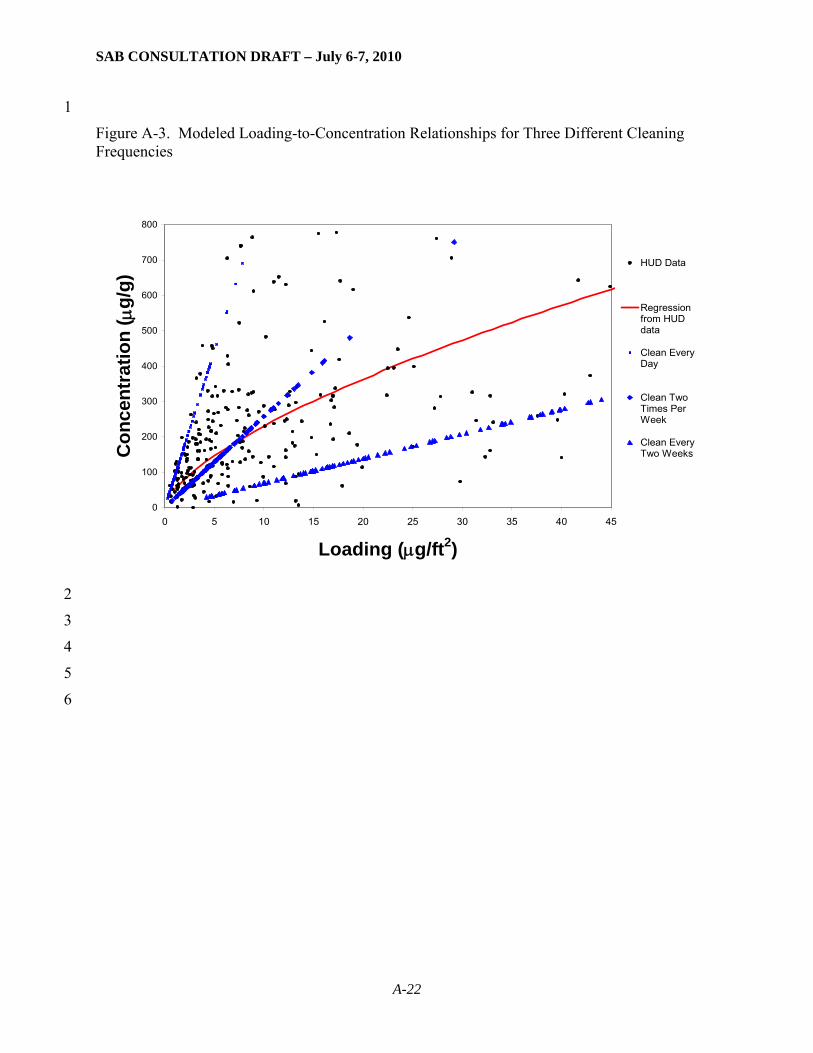
SAB CONSULTATION DRAFT – July 6-7, 2010
1
Figure A-3. Modeled Loading-to-Concentration Relationships for Three Different Cleaning Frequencies
0
100
200
300
400
500
600
700
800
0 5 10 15 20 25 30 35 40 45
Loading (μg/ft2)
Con
cent
ratio
n ( μ
g/g)
HUD Data
Regressionfrom HUDdata
Clean EveryDay
Clean TwoTimes PerWeek
Clean EveryTwo Weeks
2
3
4
5
6
A-22

SAB CONSULTATION DRAFT – July 6-7, 2010
Figure A-4. Modeled Loading and Concentration Values Using HUD Air, Paint, and Soil Distributions and Distributions for Soil Tracking and Cleaning Frequency
0
100
200
300
400
500
600
700
800
0 5 10 15 20 25 30 35 40 45
Loading (μg/ft2)
Con
cent
ratio
n ( μ
g/g)
HUD Data
Regressionfrom HUDdata
Model
1
Table A-7. Comparison Between Modeled and Actual Loadings and Concentrations
Mean Load
Mean Concen
Median Load
Median Concen
HUD Data 21 559 7.4 201
Model 13 336 7.3 188
2
Table A-8. Comparison Between Modeled and Actual Loadings and Concentrations
% Air % Soil % Paint
Indoor / Outdoor Air Ratio
% Indoor Dust from Organic
Sources Literature 17%1 49%1 34%1 0.72 42% +/- 17%3 Model 38% 13% 49% 0.63 66% 1 From Adgate et al. (1998) 2 From Colome et al. (1992) 3 From Allott et al. (1994)
A-23

SAB CONSULTATION DRAFT – July 6-7, 2010
1
2 3 4 5 6 7 8 9
10 11 12 13 14 15 16 17 18 19 20 21 22
23 24 25 26 27 28 29 30 31 32
Once the calibration was complete, the model was applied to a second dataset as a further model evaluation. Lanphear et al. (1998) collected data for 205 children in Rochester, NY. As part of the blood lead evaluation, they collected wipe lead dust loading samples, lead concentration samples, indoor XRF lead paint concentrations, and play yard and house perimeter lead soil samples. Samples were collected in multiple areas and a composite was estimated as the average or median sample value. Distributions were generated from the lead paint concentrations and play yard soil lead concentrations for use in the model. It was assumed that the play yard soil would be more readily tracked into the home than the house perimeter soil. The AQS monitoring network was used to calculate lead concentrations in the ambient air. A distribution was generated by finding the monthly average concentrations for data from 1993-1996 and finding the geometric mean and geometric standard deviation. The model was then applied to the dataset with no other modifications. The lead air concentration, lead soil concentration, lead paint concentration, soil tracking rate, and cleaning frequency were all sampled and modeled for 100 realizations and compared to the median of the floor lead loading and concentration estimates. Figure A-5 provides a comparison between the modeled and actual data. As in the HUD dataset, the spread and pattern of modeled data are consistent with the actual data. Note that the spread of the data is larger in the Rochester data than in the HUD data, likely due to much larger average soil concentrations. Also shown for reference is the regression line calculated from the HUD data and the regression line calculated directly from the Rochester data. The regression lines predict similar relationships at higher loadings, but differ by 25-50% for loadings between 10 and 40 μg/ft2.
Table A-9 compares the modeled and actual means and medians along with the source contribution percentages and outdoor/indoor air ratios. Overall, the model does well at predicting the medians, although it tends to underpredict the means as in the HUD dataset. Table A-10 compares other model metrics to the values in the literature. The source percentages are more similar to the Adgate data (1998), perhaps because the Rochester homes are more comparable with the Adgate Jersey City homes; however, the model still tends to contribute more from paint and less from soil than the Adgate data suggest. The indoor/outdoor ratio is still within range of the mean value from Colome et al. (1992). The percentage of dust mass arising from indoor sources is the same as in the HUD model, since this value does not rely on any of the lead media concentration values.
A-24

SAB CONSULTATION DRAFT – July 6-7, 2010
Figure A-5. Modeled Loading and Concentration Values Using Rochester Air, Paint, and Soil Distributions and Distributions for Soil Tracking and Cleaning Frequency
0
500
1000
1500
2000
2500
3000
3500
4000
0.0 20.0 40.0 60.0 80.0 100.0 120.0 140.0
Loading (μg/ft2)
Con
cent
ratio
n ( μ
g/g)
RochesterData
Regressionfrom HUD
RegressionfromRochester
Model
1
Table A-9. Comparison Between Modeled and Actual Loadings and Concentrations
Mean Load
Mean Concen
Median Load
Median Concen
Rochester Data 21 776 14 370
Model 20 590 13 342
2 3
4
5
6
7
A-25

SAB CONSULTATION DRAFT – July 6-7, 2010
Table A-10. Comparison Between Modeled and Actual Loadings and Concentrations
% Air % Soil % Paint
Indoor / Outdoor Air Ratio
% Indoor Dust from Organic
Sources Literature 17%1 49%1 34%1 0.72 42% +/- 17%3 Model 16% 27% 57% 0.63 66% 1 From Adgate et al. (1998) 2 From Colome et al. (1992) 3 From Allott et al. (1994)
1
2 3
4 5 6 7 8 9
10 11 12 13 14
15 16 17 18 19 20 21 22 23 24 25 26 27 28 29 30 31
32 33 34
A.3 Strengths and Limitations of the Loading-Concentration Conversion Models
As discussed in Section 2.3.2, each of these two alternative methods to convert the loadings to concentrations has strengths and limitations. The regression equation is based on a nationally-representative dataset with sufficient samples across different housing vintages, outdoor soil concentrations, and indoor paint concentrations. The regression equation is most reliably applied in the range of loadings and concentrations seen in the original dataset, and the hazard standard is anticipated to fall within that range. The equation is specific to residences, however, and cannot be easily extended to public and commercial buildings (see Section 3.2.3). In addition, the regression equation does not allow any incorporation of variability due to the difference in physical attributes and cleaning patterns among homes. The underlying data show a wide spread across the loading-concentration parameter space, indicating wide house-to-house variability (see Appendix A).
The mechanistic model, on the other hand, allows for extension of the model to public and commercial buildings, provided the physical processes are described adequately and the proper input values can be developed. Because the public/commercial buildings tend to be larger, more people come in and out of the buildings daily (thus introducing more dander to the indoor environment and diluting the indoor dust), and the cleaning patterns are different, these buildings can be expected to have a very different loading-to-concentration relationship than houses. However, the model assumes that the indoor environment is well-mixed and contains no concentration gradients; thus, it can be applied to any portion of the public/commercial building where this assumption is valid. The mechanistic model also allows for the loading to concentration conversion to incorporate house-to-house variability. The model is subject to uncertainty, however, because of the relatively simple form of the physical equations and the absence of information about some of the variable inputs. The model has been calibrated against the HUD dataset and then compared to one additional dataset, and the model is expected to return reasonable estimates for the national population in the range of the hazard standard. There currently is no relationship between window sill loading and concentration, however, and unless such a slope is developed, the same slope as used for the floor dust would have to be used in developing the window sill hazard standard.
In addition, the mechanistic model uses the steady state solution to the model equations. One assumption is made in the development of these equations, however, which affects the solution. When the steady state equations are solved, an assumption is made that routine cleaning happens
A-26

SAB CONS
A-27
ULTATION DRAFT – July 6-7, 2010
1 2 3 4 5 6 7 8 9
10 11 12
13 14 15 16 17 18
continuously at a rate equal to the cleaning frequency. In reality, however, the cleaning occurs in discrete episodes once per cleaning cycle. This assumption introduces some error into the slope, loading, and concentration estimates, and this error increases with increasing numbers of days between cleaning. Table A-11 shows a representative sample of the slope and loadings under the assumption of episodic and continuous cleaning for ten of the 200 model realizations. For cleaning every two weeks, the error in the slope is up to 14.5%; however, at the average cleaning frequency (about two cleanings per week), the error is only an average of 7.0% (maximum of 9.5%). The errors in the loadings are comparable, and the errors in the concentrations are only an average of 0.5% (maximum of 0.7%). Thus, this assumption, which is necessary from a practical standpoint in the development of the hazard standard in order to avoid numerous iterations of the model, introduces reasonable error in the region of anticipated cleaning frequencies.
While attempts have been made to take into account variability across homes by sampling some of the input parameters, no attempt has been made to account for variability within a home. Unlike the DIRT model (Johnson, 2008), which predicts gradients across floors and carpets, the model treats the home as a uniform environment. Differences across carpets and floors and between high traffic areas and less accessible areas are not accounted for in the model, and the assumption is made that the model captures the mean characteristics of the heterogeneous home.

SAB CONS
A-28
Table A-11. Representative Realizations Demonstrating the Error When Considering Continuous Cleaning Compared to Episodic Clean
Reali- zation
Outdoor Air
Concen. (μg/m3)
Soil Concen.
(μg/g)
Paint Concen.
(μg/g)
Tracking (g/day)
Clean. Freq. (days
between clean.)
Floor Loading, Episodic
Clean.
Floor Concen, Episodic
Clean.
Slope, Episodic
Clean.
Floor Loading, Contin. Clean.
Floor Concen. Contin. Clean.
Slope, Contin. Clean.
% Error in Load.
% Erroin
Conce
1 9.39E-02 1.39E+02 1.11E+00 9.50E-02 2.38E+00 6.04E+00 2.69E+02 2.25E-02 6.45E+00 2.67E+02 2.42E-02 6.8% -0.55 4.12E-02 6.80E+01 2.10E+00 1.78E-02 3.74E+00 7.93E+00 3.08E+02 2.58E-02 8.43E+00 3.06E+02 2.76E-02 6.3% -0.79 4.32E-03 9.61E+00 2.53E+01 1.20E-01 9.47E-01 1.80E+01 1.81E+03 9.96E-03 1.92E+01 1.80E+03 1.07E-02 6.5% -0.5
13 2.50E-02 4.41E+01 8.20E-01 1.33E-01 2.52E+00 2.87E+00 1.06E+02 2.70E-02 3.06E+00 1.06E+02 2.89E-02 6.5% -0.417 4.82E-02 7.79E+01 1.69E+00 2.79E-01 5.72E+00 1.44E+01 1.69E+02 8.49E-02 1.53E+01 1.69E+02 9.05E-02 6.3% -0.321 2.04E-02 3.69E+01 9.95E-01 3.10E-02 3.15E+00 3.28E+00 1.42E+02 2.32E-02 3.49E+00 1.41E+02 2.48E-02 6.6% -0.625 3.06E-03 7.11E+00 2.96E-01 5.28E-02 1.70E+00 4.66E-01 3.34E+01 1.39E-02 4.97E-01 3.32E+01 1.50E-02 6.6% -0.629 2.41E-02 4.27E+01 9.28E-01 7.75E-02 2.05E+00 2.30E+00 1.26E+02 1.83E-02 2.46E+00 1.25E+02 1.96E-02 6.7% -0.533 1.49E-01 2.07E+02 6.02E-01 4.05E-02 3.18E+00 8.78E+00 3.60E+02 2.44E-02 9.34E+00 3.58E+02 2.61E-02 6.4% -0.637 4.34E-01 5.24E+02 1.38E+00 5.50E-02 1.80E+00 1.44E+01 9.76E+02 1.48E-02 1.54E+01 9.70E+02 1.59E-02 6.9% -0.641 3.62E-02 6.08E+01 8.21E-01 1.27E-01 1.93E+00 2.63E+00 1.29E+02 2.04E-02 2.80E+00 1.28E+02 2.18E-02 6.4% -0.445 9.97E-03 1.98E+01 1.26E+00 5.72E-02 6.35E+00 6.67E+00 1.33E+02 5.02E-02 7.08E+00 1.32E+02 5.36E-02 6.2% -0.651 2.38E-02 4.22E+01 3.69E+00 1.46E-01 1.50E+00 4.80E+00 2.91E+02 1.65E-02 5.24E+00 2.90E+02 1.81E-02 9.1% -0.455 7.05E-02 1.08E+02 6.93E-01 2.47E-02 1.95E+00 3.10E+00 2.19E+02 1.42E-02 3.30E+00 2.17E+02 1.52E-02 6.7% -0.759 7.43E-02 1.13E+02 8.81E-01 1.26E-01 1.36E+00 2.97E+00 2.05E+02 1.45E-02 3.16E+00 2.04E+02 1.55E-02 6.5% -0.563 2.70E-01 3.48E+02 8.28E-01 2.70E-02 8.63E+00 3.76E+01 6.42E+02 5.86E-02 3.99E+01 6.38E+02 6.25E-02 6.1% -0.667 1.68E-02 3.12E+01 2.12E+00 3.84E-02 3.03E+00 5.52E+00 2.39E+02 2.31E-02 5.86E+00 2.37E+02 2.47E-02 6.2% -0.671 1.13E-01 1.64E+02 2.74E+00 4.59E-02 4.44E+00 1.66E+01 4.85E+02 3.42E-02 1.77E+01 4.82E+02 3.67E-02 6.5% -0.675 1.50E+00 1.54E+03 1.43E+00 9.95E-02 6.89E+00 1.77E+02 2.80E+03 6.31E-02 1.88E+02 2.79E+03 6.72E-02 6.1% -0.579 7.27E-02 1.11E+02 3.63E+00 4.01E-02 8.42E+00 3.00E+01 4.95E+02 6.06E-02 3.18E+01 4.92E+02 6.47E-02 6.1% -0.683 2.24E+00 2.18E+03 9.50E-01 6.81E-03 2.94E+00 9.48E+01 4.89E+03 1.94E-02 1.01E+02 4.86E+03 2.08E-02 6.4% -0.787 1.38E-03 3.57E+00 2.60E+00 1.63E-01 5.21E+00 9.80E+00 1.66E+02 5.89E-02 1.04E+01 1.66E+02 6.29E-02 6.3% -0.491 7.98E-01 8.90E+02 4.50E+00 7.50E-01 5.79E+00 2.00E+02 1.17E+03 1.71E-01 2.13E+02 1.17E+03 1.81E-01 6.1% -0.295 1.66E-01 2.27E+02 6.24E-01 5.89E-02 2.83E+00 9.01E+00 3.85E+02 2.34E-02 9.61E+00 3.83E+02 2.51E-02 6.7% -0.6
100 1.26E-01 1.79E+02 1.25E+00 1.01E-01 2.29E+00 7.48E+00 3.36E+02 2.22E-02 7.96E+00 3.34E+02 2.38E-02 6.4% -0.5
ULTATION DRAFT – July 6-7, 2010

SAB CONSULTATION DRAFT – July 6-7, 2010
A.4 Regression Relationship for Floor and Sill Dust Loadings The National Survey of Lead-Based Paint in Housing ("HUD Survey Data") was used to develop an empirical relationship between floor and window sill dust loadings. As discussed in Section A.1, in order to focus on the homes containing lead paint, only the data from the first three vintage categories were included. From the raw data, each floor and window sill dust loading was transformed by taking the natural log. Then, the regression was carried out using the untransformed variables and also the natural-log-transformed variables. Table A-12 shows the results of each regression.
Table A-12. Regression Analysis Results
Data Variable
Coefficient
Standard Error of Coefficient
t-stat p-value
F-stat, p-level
Adjusted R2
Intercept 203.8 219.6 0.93 0.35 Untransformed
Slope 21.7 4.8 4.5 <0.001 20.5, <0.001 0.064
Intercept 1.52 0.28 5.44 <0.001 Natural-log- transformed Slope 0.91 0.11 8.04 <0.001
64.6, <0.001 0.186
The data are positively skewed, and the regression analysis reveals that the log-transformed data appear more highly correlated, with a greater adjusted R2. Thus, the transformed relationship is chosen, and Figure A-6 shows the data and the regression equation. The equation relating the two loadings would then be
91.056.4 FloorSill ×= .
Figure A-6. Regression Relationship between Ln(Sill) vs Ln(Floor) for the HUD Data
A-29

SAB CONSULTATION DRAFT – July 6-7, 2010
y = 0.9067x + 1.5167R2 = 0.1864
-6
-4
-2
0
24
68
10
12
-2 -1 0 1 2 3 4 5 6 7
ln(floor loading in μg/ft2)
ln(s
ill lo
adin
g in
μg/
ft2 )
As an alternative method, Lanphear et al. (1998) collected data for 205 children in Rochester, collected in multiple locations and arithmetic and geometric averages were calculated. For the floor to sill relationship, the geometric means of floor and sill loadings were selected since they are not as susceptible to outliers within the house. As with the HUD data, regressions were performed on both the untransformed and natural-log-transformed variables. Table A-13 shows the results of each regression.
Table A-13. Regression Analysis Results
Data Variable
Coefficient
Standard Error of Coefficient
t-stat p-value
F-stat, p-level
Adjusted R2
Intercept 2583.1 3034.5 0.85 0.40 Untransformed
Slope 11.1 2.4 4.58 <0.001 21.0, <0.001 0.094
Intercept 3.1 0.64 4.86 <0.001 Natural-log- transformed Slope 0.80 0.10 7.68 <0.001
58.9, <0.001 0.234
Again, the log-transformed analysis was selected since the variables appear more highly correlated (with a greater adjusted R2), and Figure A-7 shows the data and the regression equation. In this case, the correlation is slightly higher (R=0.48) and the equation relating sill to floor loading would be
80.01.22 FloorSill ×=
A-30

SAB CONSULTATION DRAFT – July 6-7, 2010
Figure A-7. Regression Relationship between Ln(Sill) vs Ln(Floor) for the Rochester Data
y = 0.7976x + 3.0953R2 = 0.2348
0
2
4
6
8
10
12
14
0 1 2 3 4 5 6 7 8 9 10
ln(floor loading in μg/ft2)
ln(s
ill lo
adin
g in
μg/
ft2 )
A-31

SAB CONSULTATION DRAFT – July 6-7, 2010
A.5 References
Adgate, J.L., R.D. Willis, T.J. Buckley, J.C. Chow, J.G. Watson, G.G. Rhoads, and P.J.Lioy (1998). Chemical mass balance source apportionment of lead in house dust. Environ. Sci. Technol 32, 108-114.
Allott, R.W., M. Kelly, and C.N. Hewitt (1994). A model of environmental behaviour of contaminated dust and its application to determining dust fluxes and residence times. Atmos. Envir. 28 (4), 679-687.
Bero, B.N.; M.C. von Braun; I.H. von Lindern; J.E. Hammel; and R.A. Korus (1997). Evaluation of six vacuum techniques for sampling lead-containing carpeted surfaces. Advances in Environmental Research 1(3), 333-344.
CARB (2001) California Air Resources Board, Indoor Air Quality: Residential Cooking Exposures Final Assessment.
Clemson Environmental Technologies Laboratory (CETL). (2001) A Comparison of Post-Renovation and Remodeling Surface Cleaning Techniques. USEPA Office of Pollution, Prevention, and Toxics; December 14.
Colome, S.D.; Kado, N. Y.; Jaques, P; and Kleinman, M. (1992). Indoor-outdoor air pollution relations: particulate matter less than 10 μm in aerodynamic diameter (PM10) in the homes of asthmatics. Atmospheric Environment 26A, 2173-2178.
Dockery D.W. and Spengler J.D. (1981) Indoor-Outdoor Relationships of Respirable Sulfates and Particles. Atmospheric Environment. 15: 335-343.
Ewers, L.; Clark, S.; Menrath, W.; Succop, P.; Bornschein, R. (1994) Clean-Up of Lead in Household Carpet and Floor Dust. Am. Ind. Hyg. Assoc. J. 55(7): 650-657.
Freed, J. R.; , C. T.; Christie, W. N.; Carpenter, C. E. (1983) Methods for Assessing Exposure to Chemical Substance (Volume 2). EPA 560/5-1;3-015: 70-73. USEPA, Office of Toxic Substances.
Gilbert, Scott F (2003). "The Epidermis and the Origin of Cutaneous Structures". Developmental Biology. Sinauer Associates. http://www.ncbi.nlm.nih.gov/bookshelf/br.fcgi?book=dbio&part=A2929.
Johnson, D.L. (2008). A first generation dynamic ingress, redistribution and transport model of soil track-in: DIRT. Environ. Geochem. Health 30, 589-596.
Lanphear, B.P.; Burgoon, D.A.; Rust, S.W., Eberly, S; and Galke, W (1998). Environmental exposures to lead and children’s blood lead levels. Environmental Research, 76 (2): 120-130.
Layton, D.W. and P.I. Beamer (2009). Migration of contaminated soil and airborne particulates to indoor dust. Environ. Sci. Technol. 43, 8199-8205.
Liu, D. L. and Nazaroff, W. W. (2001) Modeling Pollutant Penetration Across Building Envelopes. Atmospheric Environment. 35: 4451-4462.
A-32

SAB CONSULTATION DRAFT – July 6-7, 2010
Ozkaynak, H.; Xue, J.; Spengler, J.; Wallace, L.; Pellizzari, E.; Jenkins, P. (1996) Personal Exposure to Airborne Particles and Metals: Results From the Particle TEAM Study in Riverside, California. J. Expo. Anal. Environ. Epidemiol. 6(1): 57-78.
Roberts, J.W.; G. Glass; and T.M. Spittler (1994). How much dust and lead are in an old rug-measurement and control. In Proceedings of the 6th conference of the International Society of Environmental Epidemiology and 4th Conference of the International Society for Exposure Analysis; International Society of Epidemiology: Research Triangle Park, NC.
Qian, J.; A.R. Ferro; and K.R. Fowler (2008). Estimating the resuspension rate and residence time of indoor particles. Journal of the Air and Waste Management Association 58, 502-516.
Thatcher, T. L. and Layton, D. W. (1995) Deposition, Resuspension, and Penetration of Particles Within a Residence. Atmospheric Environment. 29(13): 1487-1497.
U.S. Department of Energy (USDOE). (2001). Residential Energy Consumption Survey. http://www.eia.doe.gov/emeu/recs/recs2001/detail_tables.html.
USEPA 1995.
U.S. Environmental Protection Agency (USEPA). 1997a. Exposure Factors Handbook (Final Report). EPA/600/P-95/002F a-c. Washington, DC: Office of Research and Development; September.
U.S. Environmental Protection Agency (USEPA). 1997b. Lead Exposure Associated with Renovation and Remodeling Activities: Environmental Field Sampling Study, Volume I: Technical Report. Prepared by Battelle (Columbus, OH) for the Office of Pollution Prevention and Toxics (Washington, D.C.). EPA 747-R-96-007. May.
U.S. Environmental Protection Agency (USEPA). 1998. Risk Analysis to Support Standards for Lead in Paint, Dust, and Soil. Office of Pollution, Prevention, and Toxics. EPA 747-R-97-006. D-29 U.S. Environmental Protection Agency (USEPA). 2001. Wall Paint Exposure Model. Office of Pollution, Prevention, and Toxics. Available at http://www.epa.gov/oppt/exposure/pubs/wpemman.pdf
U.S. Environmental Protection Agency (USEPA). 2010. Air Quality System (AQS) Database. Available online at: http://www.epa.gov/ttn/airs/airsaqs/aqsweb/aqswebwarning.htm.
von Lindern, I.; Spalinger, S. M.; Bero, B. N.; Petrosyan, V.; von Braun, M. C. (2003) The Influence of Soil Remediation on Lead in House Dust. Sci. Total Environ. 303(1-2): 59-78.
Wallace, L.A. (1996) Indoor particles: A review. J. Air and Waste Management Assoc. (46)2:98-126.
A-33