Properties of the Topographic Product of Experts

Colin FyfeThe University of Paisley

Paisley, Scotlandcolin.fyfe@paisley.ac.uk

Abstract - In this paper, we show how a topographic mapping can be created from a productof experts. We learn the parameters of the mapping using gradient descent on the negativelogarithm of the probability density function of the data under the model. We show that themapping, though retaining its product of experts form, becomes more like a mixture of expertsduring training.

Key words - topographic, product of experts

1 Introduction

Recently [2], we introduced a new topology preserving mapping which we called the Topo-graphic Products of Experts (ToPoE). Based on a generative model of the experts, we showedhow a topology preserving mapping could be created from a product of experts in a mannervery similar to that used by Bishop et al [1] to convert a mixture of experts to the GenerativeTopographic Mapping (GTM).We begin with a set of experts who reside in some latent space and take responsibility forgenerating the data set. With a mixture of experts [5, 6], the experts divide up the data spacebetween them, each taking responsibility for a part of the data space. This division of labourenables each expert to concentrate on a specific part of the data set and ignore those regionsof the space for which it has no responsibility. The probability associated with any data pointis the sum of the probabilities awarded to it by the experts. There are efficient algorithms,notably the Expectation-Maximization algorithm, for finding the parameters associated withmixtures of experts. Bishop et al [1] constrained the experts’ positions in latent space andshowed that the resulting mapping also had topology preserving properties.In a product of experts, all the experts take responsibility for all the data: the probabilityassociated with any data point is the (normalised) product of the probabilities given to it bythe experts. As pointed out in e.g. [4] this enables each expert to waste probability mass inregions of the data space where there is no data, provided each expert wastes his mass in adifferent region. The most common situation is to have each expert take responsibility forhaving information about the data’s position in one dimension while having no knowledgeabout the other dimensions at all, a specific case of which is called a Gaussian pancake in[7]: a probability density function which is very wide in most dimensions but is very narrow(precisely locating the data) in one dimension. It is very elegantly associated with MinorComponents Analysis in [7].

WSOM 2005, Paris

In this paper, we review a method of creating a topology preserving mapping from a productof experts. The resulting mapping is neither a true product of experts nor a mixture ofexperts but lies somewhere in between.

2 Topographic Products of Experts

Hinton [3] investigated a product of K experts with

p(xn|Θ) ∝K∏

k=1

p(xn|k) ∝K∏

k=1

(β

2π

)D2

exp(−β

2||mk − xn||2

)(1)

where Θ is the set of current parameters in the model. Hinton notes that using Gaussiansalone does not allow us to model e.g. multi-modal distributions, however the Gaussian isideal for our purposes. To fit this model to the data we can define a cost function as thenegative logarithm of the probabilities of the data so that

C =N∑

n=1

K∑

k=1

β

2||mk − xn||2 (2)

We will, as with the GTM, allow latent points to have different responsibilities depending onthe data point presented so we use the cost function:

C1 =N∑

n=1

K∑

k=1

β

2||mk − xn||2rkn (3)

where rkn is the responsibility of the kth expert for the data point, xn. Thus all the experts areacting in concert to create the data points but some will take more responsibility than others.Note how crucial the responsibilities are in this model: if an expert has no responsibility for aparticular data point, it is in essence saying that the data point could have a high probabilityas far as it is concerned. We do not allow a situation to develop where no expert acceptsresponsibility for a data point; if no expert accepts responsibility for a data point, they all aregiven equal responsibility for that data point (see below). For comparison, the probability ofa data point under the GTM is

p(x) =K∑

i=1

P (i)p(x|i) =K∑

i=1

1K

(β

2π

)D2

exp(−β

2||mi − x||2

)(4)

We wish to maximise the likelihood of the data set X = {xn : n = 1, · · · , N} under thismodel. The ToPoE learning rule (6) is derived from the minimisation of C1 with respect toa set of parameters which generate the mk.We now turn our attention to the nature of the K experts which are going to generate the Kcentres, mk. We envisage that the underlying structure of the experts can be represented byK latent points, t1, t2, · · · , tK . To allow local and non-linear modeling, we map those latentpoints through a set of M basis functions, f1(), f2(), · · · , fM (). This gives us a matrix Φ whereφkj = fj(tk). Thus each row of Φ is the response of the basis functions to one latent point, oralternatively we may state that each column of Φ is the response of one of the basis functions

Properties of the Topographic Product of Experts

to the set of latent points. One of the functions, fj(), acts as a bias term and is set to onefor every input. Typically the others are gaussians centered in the latent space. The outputof these functions are then mapped by a set of weights, W , into data space. W is M × D,where D is the dimensionality of the data space, and is the sole parameter which we changeduring training. We will use wi to represent the ith column of W and Φj to represent the rowvector of the mapping of the jth latent point. Thus each basis point is mapped to a point indata space, mj = ΦjW .We may update W either in batch mode or with online learning. To change W in onlinelearning, we randomly select a data point, say xi. We calculate the current responsibility ofthe jth latent point for this data point,

rij =exp(−γd2

ij)∑k exp(−γd2

ik)(5)

where dpq = ||xp−mq||, the euclidean distance between the pth data point and the projectionof the qth latent point (through the basis functions and then multiplied by W). If no weightsare close to the data point (the denominator of (5) is zero), we set rij = 1

K ,∀j.Define m

(k)d =

∑Mm=1 wmdφkm, i.e. m

(k)d is the projection of the kth latent point on the dth

dimension in data space. Similarly let x(n)d be the dth coordinate of xn. These are used in

the update rule

∆nwmd =K∑

k=1

ηφkm(x(n)d −m

(k)d )rkn (6)

where we have used ∆n to signify the change due to the presentation of the nth data point,xn, so that we are summing the changes due to each latent point’s response to the datapoints. Note that, for the basic model, we do not change the Φ matrix during training atall. It is the combination of the fact that the latent points are mapped through the basisfunctions and that the latent points are given fixed positions in latent space which gives theToPoE its topographic properties. We have previously illustrated these on artificial data in[2].

3 Product or Mixture?

A model based on products of experts has some advantages and disadvantages. The majordisadvantage is that no efficient EM algorithm exists for optimising parameters. [3] suggestsusing Gibbs sampling but even with the very creative method discussed in that paper, thesimulation times were excessive. Thus we have opted for gradient descent as the parameteroptimisation method.The major advantage which a product of experts method has is that it is possible to get verymuch sharper probability density functions with a product rather than a sum of experts.The responsibilities are adapting the width of each expert locally dependent on both theexpert’s current projection into data space and the data point for which responsibility mustbe taken. Initially, rkn = 1

K ,∀k, n and so we have the standard product of experts. Howeverduring training, the responsibilities are refined so that individual latent points take moreresponsibility for specific data points. We may view this as the model softening from a trueproduct of experts to something between that and a mixture of experts.

WSOM 2005, Paris

0

5

10

15

20

0

100

200

300

400

5000

0.2

0.4

0.6

0.8

1

Responsibilities

iteration *100 latent point

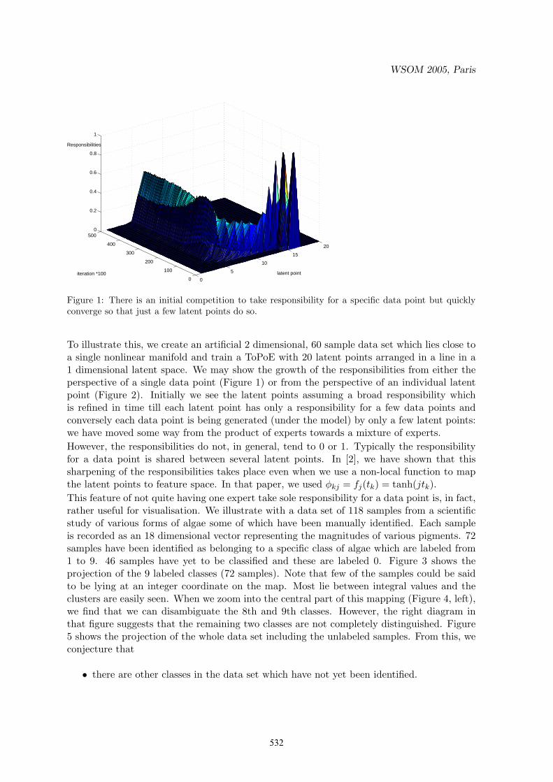
Figure 1: There is an initial competition to take responsibility for a specific data point but quicklyconverge so that just a few latent points do so.

To illustrate this, we create an artificial 2 dimensional, 60 sample data set which lies close toa single nonlinear manifold and train a ToPoE with 20 latent points arranged in a line in a1 dimensional latent space. We may show the growth of the responsibilities from either theperspective of a single data point (Figure 1) or from the perspective of an individual latentpoint (Figure 2). Initially we see the latent points assuming a broad responsibility whichis refined in time till each latent point has only a responsibility for a few data points andconversely each data point is being generated (under the model) by only a few latent points:we have moved some way from the product of experts towards a mixture of experts.However, the responsibilities do not, in general, tend to 0 or 1. Typically the responsibilityfor a data point is shared between several latent points. In [2], we have shown that thissharpening of the responsibilities takes place even when we use a non-local function to mapthe latent points to feature space. In that paper, we used φkj = fj(tk) = tanh(jtk).This feature of not quite having one expert take sole responsibility for a data point is, in fact,rather useful for visualisation. We illustrate with a data set of 118 samples from a scientificstudy of various forms of algae some of which have been manually identified. Each sampleis recorded as an 18 dimensional vector representing the magnitudes of various pigments. 72samples have been identified as belonging to a specific class of algae which are labeled from1 to 9. 46 samples have yet to be classified and these are labeled 0. Figure 3 shows theprojection of the 9 labeled classes (72 samples). Note that few of the samples could be saidto be lying at an integer coordinate on the map. Most lie between integral values and theclusters are easily seen. When we zoom into the central part of this mapping (Figure 4, left),we find that we can disambiguate the 8th and 9th classes. However, the right diagram inthat figure suggests that the remaining two classes are not completely distinguished. Figure5 shows the projection of the whole data set including the unlabeled samples. From this, weconjecture that

• there are other classes in the data set which have not yet been identified.

Properties of the Topographic Product of Experts

0

10

20

30

40

50

60

0

100

200

300

400

5000

0.2

0.4

0.6

0.8

1

Responsibilities

Data points

Iterations *100

Figure 2: The latent point initially has broad responsibilities but learns to take responsibility for onlya few data points.

• some of the unclassified samples belong to classes already identified.

• some may be simply outliers.

These are, however, speculations on our part and must be validated by a scientist withbiological expertise.It is of interest to compare the GTM on the same data: we use a two dimensional latentspace with a 10×10 grid for comparison. The results are shown in Figure 6. The GTMmakes a very confident classification: we see that the responsibilities for data points are veryconfidently assigned in that individual classes tend to be allocated to a single latent point.This, however works against the GTM in that, even with zooming in to the map, one cannotsometimes disambiguate the two different classes such as at the points (1,-1) and (1,1). Thiswas not alleviated by using regularisation in the GTM though we should point out that wehave a very powerful model for a rather small data set.In fact, we can control the level of quantisation by changing the γ parameter in (5). Forexample by lowering γ, we share the responsibilities more equally and so the map contractsto the centre of the latent space to get results such as shown in Figure 7; the different clusterscan still be identified but rather less easily. Alternately, by increasing γ, one tends to get thedata clusters confined to a single node, that which has sole responsibility for that cluster.We are, in effect, able to control how much our product of experts mapping moves towardsa mixture of experts.

References

[1] C. M. Bishop, M. Svensen, and C. K. I. Williams. Gtm: The generative topographicmapping. Neural Computation, 1997.

WSOM 2005, Paris

0 1 2 3 4 5 6 7 8 90

1

2

3

4

5

6

7

8

99 species of algae

Figure 3: Projection of the 9 classes by the ToPoE.

5.3 5.4 5.5 5.6 5.7 5.8

4

4.2

4.4

4.6

4.8

5

Zooming in on the central portion

0.2 0.4 0.6 0.8 1 1.2 1.42.5

3

3.5

4

4.5

5

5.5

Second zoom

Figure 4: Left: zooming in on the central portion. Right: zooming in on the left side.

Properties of the Topographic Product of Experts

0 1 2 3 4 5 6 7 8 90

1

2

3

4

5

6

7

8

9Using the unclassified algae

outlier ?

outlier ?

outlier ?

New class?

type 3 ?

Figure 5: The projection of the whole data set by the ToPoE.

−1 −0.8 −0.6 −0.4 −0.2 0 0.2 0.4 0.6 0.8 1−1

−0.8

−0.6

−0.4

−0.2

0

0.2

0.4

0.6

0.8

1The GTM is very sure

Figure 6: The projection of the algae data given by the GTM.

WSOM 2005, Paris

4.46 4.47 4.48 4.49 4.5 4.51 4.52 4.53 4.544.46

4.47

4.48

4.49

4.5

4.51

4.52

4.53

4.54

4.55

Figure 7: By lowering the γ parameter, the ToPoE map is contracted.

[2] C. Fyfe. Topographic product of experts. In International Conference on Artificial NeuralNetworks, ICANN2005, 2005.

[3] G. E. Hinton. Training products of experts by minimizing contrastive divergence. Tech-nical Report GCNU TR 2000-004, Gatsby Computational Neuroscience Unit, UniversityCollege, London, http://www.gatsby.ucl.ac.uk/, 2000.

[4] G.E. Hinton and Y.-W. Teh. Discovering multiple constraints that are frequently approx-imately satisfied. In Proceedings of the Seventh Conference on Uncertainty in ArtificialIntelligence, pages 227–234, 2001.

[5] R.A. Jacobs, M.I. Jordan, S.J. Nowlan, and G.E. Hinton. Adaptive mixtures of localexperts. Neural Computation, 3:79–87, 1991.

[6] M.I. Jordan and R.A. Jacobs. Hierarchical mixtures of experts and the em algorithm.Neural Computation, 6:181–214, 1994.

[7] C. Williams and F. V. Agakov. Products of gaussians and probabilistic minor componentsanalysis. Technical Report EDI-INF-RR-0043, University of Edinburgh, 2001.