Properties of Stable Matchings

by

Michael Jay Szestopalow

A thesispresented to the University of Waterloo

in fulfillment of thethesis requirement for the degree of

Master of Mathematicsin

Combinatorics and Optimization

Waterloo, Ontario, Canada, 2010

c© Michael Jay Szestopalow 2010

I hereby declare that I am the sole author of this thesis. This is a true copy of the thesis,including any required final revisions, as accepted by my examiners.

I understand that my thesis may be made electronically available to the public.

iii

Abstract

Stable matchings were introduced in 1962 by David Gale and Lloyd Shapley to studythe college admissions problem. The seminal work of Gale and Shapley has motivated hun-dreds of research papers and found applications in many areas of mathematics, computerscience, economics, and even medicine. This thesis studies stable matchings in graphs andhypergraphs.

We begin by introducing the work of Gale and Shapley. Their main contribution was theproof that every bipartite graph has a stable matching. Our discussion revolves around theGale-Shapley algorithm and highlights some of the interesting properties of stable match-ings in bipartite graphs. We then progress to non-bipartite graphs. Contrary to bipartitegraphs, we may not be able to find a stable matching in a non-bipartite graph. Some ofthe work of Irving will be surveyed, including his extension of the Gale-Shapley algorithm.Irving’s algorithm shows that many of the properties of bipartite stable matchings remainwhen the general case is examined.

In 1991, Tan showed how to extend the fundamental theorem of Gale and Shapley tonon-bipartite graphs. He proved that every graph contains a set of edges that is very similarto a stable matching. In the process, he found a characterization of graphs with stablematchings based on a modification of Irving’s algorithm. Aharoni and Fleiner gave a non-constructive proof of Tan’s Theorem in 2003. Their proof relies on a powerful topologicalresult, due to Scarf in 1965. In fact, their result extends beyond graphs and shows thatevery hypergraph has a fractional stable matching. We show how their work provides newand simpler proofs to several of Tan’s results.

We then consider fractional stable matchings from a linear programming perspective.Vande Vate obtained the first formulation for complete bipartite graphs in 1989. Fur-ther, he showed that the extreme points of the solution set exactly correspond to stablematchings. Roth, Rothblum, and Vande Vate extended Vande Vate’s work to arbitrarybipartite graphs. Abeledo and Rothblum further noticed that this new formulation canmodel fractional stable matchings in non-bipartite graphs in 1994. Remarkably, theseformulations yield analogous results to those obtained from Gale-Shapley’s and Irving’salgorithms. Without the presence of an algorithm, the properties are obtained throughclever applications of duality and complementary slackness.

We will also discuss stable matchings in hypergraphs. However, the desirable propertiesthat are present in graphs no longer hold. To rectify this problem, we introduce a new“majority” stable matchings for 3-uniform hypergraphs and show that, under this strongerdefinition, many properties extend beyond graphs. Once again, the linear programmingtools of duality and complementary slackness are invaluable to our analysis. We willconclude with a discussion of two open problems relating to stable matchings in 3-uniformhypergraphs.

v

Acknowledgements

First and foremost, I wish to thank Penny Haxell. This thesis would not exist without herunwavering encouragement and endless patience.

I would like to thank Nick Harvey and Steve Furino for their time and comments relatedto this thesis. A very special thanks to Jeanne Youlden for her generous contribution thathelped make it financially possible for me to continue my studies. Finally, I would like tothank Cathy Brown for helping to conceal my neglect of the English language.

vii

Dedication

For my parents, Janie and Victor.

ix

Table of Contents

List of Figures xiii

List of Tables xv

List of Algorithms xvii

1 Introduction 1

1.1 Background Check . . . . . . . . . . . . . . . . . . . . . . . . . . . . . . . 5

1.1.1 Graph Theory . . . . . . . . . . . . . . . . . . . . . . . . . . . . . . 5

1.1.2 Linear Programming . . . . . . . . . . . . . . . . . . . . . . . . . . 7

1.1.3 Order Theory . . . . . . . . . . . . . . . . . . . . . . . . . . . . . . 10

2 Stable Matchings in Graphs 13

2.1 Bipartite Graphs . . . . . . . . . . . . . . . . . . . . . . . . . . . . . . . . 14

2.1.1 The Gale-Shapley Algorithm . . . . . . . . . . . . . . . . . . . . . . 15

2.1.2 The Lattice of Stable Matchings . . . . . . . . . . . . . . . . . . . . 18

2.2 Non-Bipartite Graphs . . . . . . . . . . . . . . . . . . . . . . . . . . . . . . 20

2.2.1 Irving’s Algorithm . . . . . . . . . . . . . . . . . . . . . . . . . . . 22

2.3 Consequences of Irving’s Algorithm . . . . . . . . . . . . . . . . . . . . . . 28

3 Fractional Stable Matchings 31

3.1 Scarf’s Lemma . . . . . . . . . . . . . . . . . . . . . . . . . . . . . . . . . 32

3.2 Stable Partitions . . . . . . . . . . . . . . . . . . . . . . . . . . . . . . . . 34

xi

3.2.1 Tan’s Algorithm . . . . . . . . . . . . . . . . . . . . . . . . . . . . . 37

3.2.2 A Consequence of Tan’s Algorithm . . . . . . . . . . . . . . . . . . 41

3.3 Linear Programming . . . . . . . . . . . . . . . . . . . . . . . . . . . . . . 42

3.3.1 Stable Matchings and Linear Programming . . . . . . . . . . . . . . 43

4 3-Uniform Hypergraphs 47

4.1 Difficulties with Hypergraph Stable Matchings . . . . . . . . . . . . . . . . 48

4.2 Majority Stable Matchings . . . . . . . . . . . . . . . . . . . . . . . . . . . 50

4.2.1 Constructing Majority Stable Matchings . . . . . . . . . . . . . . . 58

5 Concluding Remarks 63

5.1 Open Questions . . . . . . . . . . . . . . . . . . . . . . . . . . . . . . . . . 64

5.1.1 The Cyclic Stable Family Problem . . . . . . . . . . . . . . . . . . 64

5.1.2 Bounded Denominators . . . . . . . . . . . . . . . . . . . . . . . . . 68

Bibliography 74

xii

List of Figures

1.1 Example of a graph . . . . . . . . . . . . . . . . . . . . . . . . . . . . . . . 5

1.2 Example of a directed graph . . . . . . . . . . . . . . . . . . . . . . . . . . 6

1.3 Example of a non-maximal matching . . . . . . . . . . . . . . . . . . . . . 6

1.4 Example of a bipartite graph . . . . . . . . . . . . . . . . . . . . . . . . . . 7

1.5 Convex and non-convex sets . . . . . . . . . . . . . . . . . . . . . . . . . . 9

1.6 Hasse diagram . . . . . . . . . . . . . . . . . . . . . . . . . . . . . . . . . . 10

2.1 Example of a stable matching . . . . . . . . . . . . . . . . . . . . . . . . . 14

2.2 Bipartite graph with 10 stable matchings . . . . . . . . . . . . . . . . . . . 18

2.3 Stable matchings M1 (thicker edges) and M2 . . . . . . . . . . . . . . . . . 19

2.4 Hasse diagram of stable matchings . . . . . . . . . . . . . . . . . . . . . . 20

2.5 Example with no stable matchings . . . . . . . . . . . . . . . . . . . . . . 21

2.6 K6 with preferences . . . . . . . . . . . . . . . . . . . . . . . . . . . . . . . 23

2.7 Phase 1 subgraph . . . . . . . . . . . . . . . . . . . . . . . . . . . . . . . . 23

2.8 Removing a rotation . . . . . . . . . . . . . . . . . . . . . . . . . . . . . . 25

2.9 Example of a graph with poset preferences . . . . . . . . . . . . . . . . . . 29

2.10 A problem with poset preferences . . . . . . . . . . . . . . . . . . . . . . . 29

2.11 Poset preferences and stable matchings of different size . . . . . . . . . . . 30

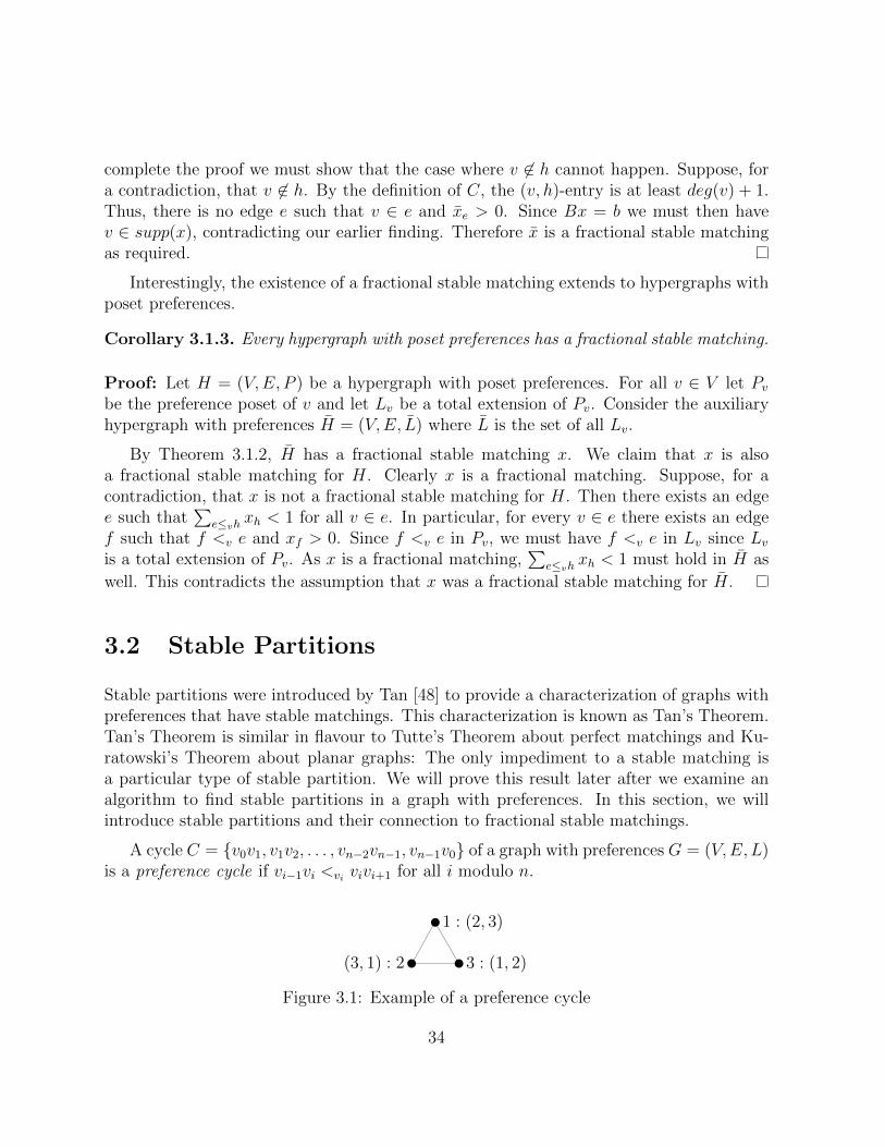
3.1 Example of a preference cycle . . . . . . . . . . . . . . . . . . . . . . . . . 34

3.2 Example of non-convex fractional stable matchings . . . . . . . . . . . . . 42

4.1 Starting the construction of H(G; M) . . . . . . . . . . . . . . . . . . . . . 59

xiii

List of Tables

4.1 Example of a hypergraph . . . . . . . . . . . . . . . . . . . . . . . . . . . . 48

4.2 Stable matchings of different size . . . . . . . . . . . . . . . . . . . . . . . 49

4.3 No vertex partition . . . . . . . . . . . . . . . . . . . . . . . . . . . . . . . 49

4.4 No half-integral stable matching . . . . . . . . . . . . . . . . . . . . . . . . 49

4.5 Majority stable matching example . . . . . . . . . . . . . . . . . . . . . . . 51

4.6 Feasible set of (PMSM) can be empty . . . . . . . . . . . . . . . . . . . . . 52

4.7 Construction of H(G; M) . . . . . . . . . . . . . . . . . . . . . . . . . . . . 59

4.8 Preference lists of N(X) in H and H[N(X)] . . . . . . . . . . . . . . . . . 61

xv

List of Algorithms

1 Gale-Shapley Algorithm . . . . . . . . . . . . . . . . . . . . . . . . . . . . 152 Irving’s Algorithm - Phase 1 . . . . . . . . . . . . . . . . . . . . . . . . . . 223 Irving’s Algorithm - Phase 2 . . . . . . . . . . . . . . . . . . . . . . . . . . 264 Tan’s Algorithm - Phase 1 . . . . . . . . . . . . . . . . . . . . . . . . . . . 385 Tan’s Algorithm - Phase 2 . . . . . . . . . . . . . . . . . . . . . . . . . . . 40

xvii

Chapter 1

Introduction

Imagine that you travel back through time to your final year of high school. It is anexciting time: The days of walking down the halls towards those “decidedly useless” classesare coming to a triumphant end. In the background, school counsellors can be foundpreaching the importance of a post-secondary education. Not surprisingly, we will assumethat you are one of the best students in your school. Because of this assumption, the schoolcounsellors are particularly interested in seeing you attend a post-secondary school and,eventually, have a profound impact on the rest of the world. Try as you may, you reallywill not find a better alternative. Wisely, you accept this idea without too much trouble.You will ultimately be faced with three questions.

The first of these questions is arguably the most important: “Which post-secondaryinstitution should I choose to take all of my money?” The answer will not be found easily;factors such as tuition costs, distance from home, and program reputation will undoubtedlyaffect your eventual choice of school. From the other side, a university has to decidewhich students it will admit. Naturally, a school would want to admit the best studentspossible. However, this may not happen since the best students could prefer to attendanother school. To help with this problem, imagine the existence of a central admissionscommittee that assigns students to schools based on the preferences of both. In addition,suppose Rebecca applied for admission to the University of Waterloo. Ideally, this centraladmissions committee would like to avoid the situation in which Rebecca is denied entry toUW, but would rather admit her than some other student who has already been accepted.Such a scenario would undermine the credibility of the committee since both the studentand the school would have a reason to ignore the committee’s decision.

The second question you will be faced with is: “Who am I going to be yelling at forspawning a new type of bacteria ten feet from where I sleep?” Once a school has a final listof its new first-year students, it now has the task of assigning roommates for the students

1

living in residence. Similar to the first problem, the school does not want students takingmatters into their own hands and reorganizing their living arrangements.

The final question comes after four years of hard work and many hours of lost sleepwhen you finally graduate with a post-secondary degree. You are now expected to starta life in the real world. Typically, this life will involve a successful career (your recentlyobtained degree will be useful in this endeavour) and, more relevant for this paper, abeautiful family. The question becomes: “Who am I going to spend the rest of my lifewith?”

These questions motivate the following three problems:

Problem 1 (College Admissions Problem). A set of n high school students are applying tom universities. Naturally, each student can attend only one university and each universityhas some maximum quota of students. Students rank universities to which they apply,and each university ranks its applicants. Can we find an assignment of students to schoolssuch that if a student is not attending a particular university, then either the studentis attending a school he prefers, or the university has reached its admissions quota withstudents it prefers?

Problem 2 (Stable Roommates Problem). Suppose there are n people living in a universitydormitory. Each person ranks the other students in terms of who they would prefer to haveas a roommate. Can we find an assignment of roommates such that if two people are notroommates then at least one of them prefers their current roommate?

Problem 3 (Stable Marriage Problem). A community consists of n men and m women.Each person ranks members of the opposite sex in terms of who they would prefer for aspouse. Can we find a set of couples such that if two people are not married to each otherthen at least one of them prefers their spouse?

Notice that the stable marriage problem is a special case of the college admissionsproblem: Imagine that each university is only allowed to admit a single student. This isa ludicrous notion; the tuition fees of those poor students would be astronomical! Fortu-nately, this is where the marriage metaphor becomes useful. Restricting each university toonly one student, while ridiculous in principle, yields the stable marriage problem.

We can view the stable marriage problem as an attempt to prevent affairs amongmarried partners. While this is a noble cause, the recent “transgressions” of a certainprofessional golfer would suggest that preventing affairs is an impossible task. Needless tosay, there are social reasons why the stable marriage problem may not accurately describesuccessful marriages, but we will not delve into such reasons here. However, the NationalResident Matching Program (NRMP) is a real example where these problems find someuse.

2

Similar to post-doctoral fellows, residents are recently graduated medical doctors whopractice medicine under the supervision of a full physician until they have the experienceto work as physicians themselves. The NRMP began in 1952 to match residents withhospitals based on the preferences of the participating parties. In fact, they try to solvethe college admissions problem. Indeed, there is no shortage of examples of these two-sidedpreference models. Here at the University of Waterloo we can look to the Co-operativeEducation program: After their interviews, students rank potential employers in terms ofwork preference and the employers rank their student applicants.

Our three problems were formally introduced in 1962 by David Gale and Lloyd Shap-ley [13] and fall into the class of stable matching problems. The main contribution ofGale and Shapley was their proof that every instance of the college admissions problem,and therefore the stable marriage problem, has a solution. Their proof was based on analgorithm we will see later in Section 2.1.1.

Sadly, Gale and Shapley found the following example to show that an instance ofthe stable roommates problem may not have a solution: Suppose a dormitory consists ofAndrew, Brandon, Christopher, and David. Andrew ranks Brandon first, Brandon ranksChristopher first, Christopher ranks Andrew first, and all three rank David last. David’spreferences are immaterial at this point. David’s roommate, regardless of who it is, willprefer both of the others, and one of those two will also prefer David’s roommate [13].Thus, there is no stable assignment of roommates.

However, the seminal work of Gale and Shapley has motivated some fascinating math-ematics, and has been the starting point for hundreds of research papers. In a series oflectures in 1976, Donald Knuth [33] showed that the set of all stable matchings in a bi-partite graph forms a distributive lattice. Although this fact was largely ignored for manyyears, it eventually led to some remarkable consequences. Knuth also conjectured thatstable matchings and lattice theory might be more closely related than originally thought.We will see in Section 2.1.2 that this is indeed the case. As another example, the theoryof stable matchings can be used to give a short proof of Galvin’s Theorem for list-edge-colourings of bipartite multi-graphs, and hence, a proof of the Dinitz conjecture aboutpartial Latin squares [16].

In the last five years, applications of stable matchings have found their way back tothe medical fields. In particular, variants of stable matching problems have been used tomodel the so-called kidney transplant problem. This is essentially the problem of matchingpatients to donors where the preferences for a patient needing a kidney are based on thesuitability of the potential donors [24, 43].

Obviously, the main objective of this thesis is to examine some of the interesting math-ematical properties of stable matchings. Consequently, the bulk of our discussion will bean exposition of the works of Gale and Shapley, Knuth, Irving, and many others. Un-fortunately, a common trait among stable matching papers is that many are written in

3

the context of computer science. While it is undeniable that there have been many ad-vancements in stable matching research, this language can be unfamiliar to certain aspiringmathematicians. We will try to present this material in the context of graph theory andlimit the use of the lists and tables of computer science. Hopefully, this will clean up thepresentation of many of the proofs.

Section 1.1 will conclude our introduction with a review of the necessary prerequisitematerial from graph theory, linear programming, and order theory.

In Chapter 2 we will introduce the stable matching problem. Starting with the workof Gale and Shapley, we highlight some of the interesting properties of stable matchings inbipartite graphs. The chapter will conclude with a look at stable matchings in non-bipartitegraphs. We will see that we keep many of the properties of bipartite stable matchings whenwe jump to the general case.

The purpose of Chapter 3 will be to show that the fundamental theorem of Gale andShapley from Chapter 2 can be extended to non-bipartite graphs by considering a suitableextension of stable matchings. We will consider a result of Tan, and a subsequent resultof Aharoni and Fleiner, which shows that every graph contains a set of edges that is verysimilar to a stable matching. This special set of edges will allow us to characterize thegraphs that have stable matchings. We will also take a vacation from the combinatorialside of stable matchings to visit the linear programming world. Duality and complementaryslackness can provide alternate proofs to many of the results of Chapter 2.

Chapter 4 will bring stable matchings to 3-uniform hypergraphs. We will highlight someof the difficulties stable matchings present us when we move from graphs to hypergraphsand discuss some open questions and conjectures. To deal with these difficulties, we proposea new, stronger, definition of stable matching. Using techniques from linear programming,we obtain original results that show the behaviour of these “majority” stable matchingsmirrors the behaviour of stable matchings in graphs more closely than the standard stablematching in 3-uniform hypergraphs. We will also construct a very large class of 3-uniformhypergraphs admitting a majority stable matching.

Chapter 5 highlights two open questions about stable matchings in 3-uniform hyper-graphs. The first asks if there is always a stable matching when the preferences are struc-tured in a specific way. The second asks if every 3-uniform hypergraph has a fractionalstable matching where all the edge values are not too small. For both problems, we provethat small instances have a positive answer.

4

1.1 Background Check

Possibly excepting some of the order theory, most undergraduates in the Department ofCombinatorics and Optimization here at the University of Waterloo will have seen all ofthis background material by the time they finish the third year of their studies. For thisreason, the majority of people who voluntarily read this thesis can skip the remainder ofthis chapter. However, we include our background section should a reader need a briefreview of basic graph theory, linear optimization, or order theory.

1.1.1 Graph Theory

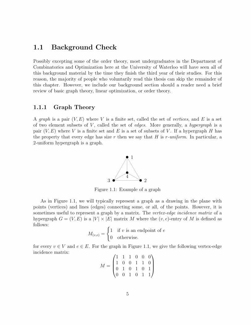
A graph is a pair (V,E) where V is a finite set, called the set of vertices, and E is a setof two element subsets of V , called the set of edges. More generally, a hypergraph is apair (V,E) where V is a finite set and E is a set of subsets of V . If a hypergraph H hasthe property that every edge has size r then we say that H is r-uniform. In particular, a2-uniform hypergraph is a graph.

1

234

Figure 1.1: Example of a graph

As in Figure 1.1, we will typically represent a graph as a drawing in the plane withpoints (vertices) and lines (edges) connecting some, or all, of the points. However, it issometimes useful to represent a graph by a matrix. The vertex-edge incidence matrix of ahypergraph G = (V,E) is a |V | × |E| matrix M where the (v, e)-entry of M is defined asfollows:

M(v,e) =

{1 if v is an endpoint of e

0 otherwise.

for every v ∈ V and e ∈ E. For the graph in Figure 1.1, we give the following vertex-edgeincidence matrix:

M =

1 1 1 0 0 01 0 0 1 1 00 1 0 1 0 10 0 1 0 1 1

5

In a graph, a vertex v is a neighbour of vertex u if uv ∈ E. The neighbourhood of avertex u, denoted N(u), is the set of neighbours of u. Let v ∈ V . The degree of v, denoteddeg(v), is defined to be the number of edges e such that v is an endpoint of e. If deg(u) = 0for some vertex u then we say that u is isolated. Note that in a graph, an isolated vertexhas an empty neighbourhood.

A directed graph, or digraph, is a pair (N,A) where N is a finite set of nodes and A isa set of ordered pairs of distinct nodes of N , called arcs. The distinction here is that thearcs have a direction associated with them: If a = (u, v) is an arc, we think of the arc asbeing directed from u to v. Therefore, in Figure 1.2, we see that the arcs (2, 3) and (3, 2)are different. Alternatively, we will say that u is the tail of arc a and v is the head of a;these will be denoted by tail(a) and head(a), respectively.

1

23

4

Figure 1.2: Example of a directed graph

Let G = (V,E) be a hypergraph. We say H = (V , E) is a subhypergraph of G if V ⊆ Vand E ⊆ E. We will often denote V (H) and E(H) to be the vertices and edges of thesubhypergraph, respectively.

A matching in a hypergraph G = (V,E) is a set of edges, M ⊆ E, such that each vertexin V is incident to at most one edge of M . A matching M is maximal if M ∪ e is not amatching for any e ∈ E\M . In Figure 1.3, the matching is not maximal since we couldadd the edge 34 to obtain a larger matching. Further, if every vertex is incident to exactlyone edge of M , then M is a perfect matching.

1

234

Figure 1.3: Example of a non-maximal matching

A graph G = (V,E) is bipartite if there is a partition (A,B) of V such that everyedge of E has exactly one endpoint in A and one endpoint in B. Similarly, a 3-uniform

6

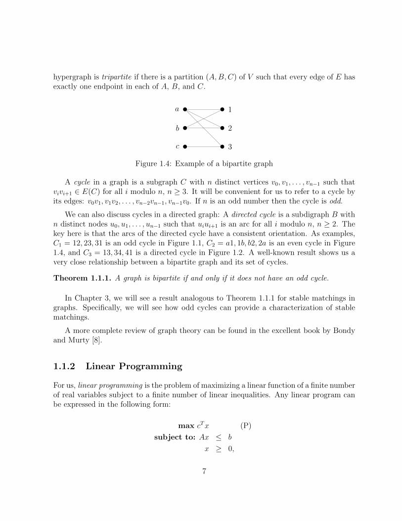
hypergraph is tripartite if there is a partition (A,B,C) of V such that every edge of E hasexactly one endpoint in each of A, B, and C.

1

2

3

a

b

c

Figure 1.4: Example of a bipartite graph

A cycle in a graph is a subgraph C with n distinct vertices v0, v1, . . . , vn−1 such thatvivi+1 ∈ E(C) for all i modulo n, n ≥ 3. It will be convenient for us to refer to a cycle byits edges: v0v1, v1v2, . . . , vn−2vn−1, vn−1v0. If n is an odd number then the cycle is odd.

We can also discuss cycles in a directed graph: A directed cycle is a subdigraph B withn distinct nodes u0, u1, . . . , un−1 such that uiui+1 is an arc for all i modulo n, n ≥ 2. Thekey here is that the arcs of the directed cycle have a consistent orientation. As examples,C1 = 12, 23, 31 is an odd cycle in Figure 1.1, C2 = a1, 1b, b2, 2a is an even cycle in Figure1.4, and C3 = 13, 34, 41 is a directed cycle in Figure 1.2. A well-known result shows us avery close relationship between a bipartite graph and its set of cycles.

Theorem 1.1.1. A graph is bipartite if and only if it does not have an odd cycle.

In Chapter 3, we will see a result analogous to Theorem 1.1.1 for stable matchings ingraphs. Specifically, we will see how odd cycles can provide a characterization of stablematchings.

A more complete review of graph theory can be found in the excellent book by Bondyand Murty [8].

1.1.2 Linear Programming

For us, linear programming is the problem of maximizing a linear function of a finite numberof real variables subject to a finite number of linear inequalities. Any linear program canbe expressed in the following form:

max cTx (P)

subject to: Ax ≤ b

x ≥ 0,

7

where A ∈ Rm×n, c ∈ Rn, and b ∈ Rm. This is called the primal problem. A feasiblesolution of (P) is a vector x ∈ Rn such that Ax ≤ b and x ≥ 0. A feasible solution, x∗, isan optimal solution of (P) if cTx∗ ≥ cTx for every feasible solution, x, of (P). Associatedwith (P) is another linear program:

min bTy (D)

subject to: ATy ≥ c

y ≥ 0.

This is the dual linear program. The feasible solutions of (P) have a special relationshipwith the feasible solutions of (D).

Lemma 1.1.2 (Weak Duality). If x is a feasible solution to (P) and y is a feasible solutionto (D), then cT x ≤ bT y.

Corollary 1.1.3. If x is a feasible solution to (P), y is a feasible solution to (D), andcT x = bT y, then x is optimal for (P) and y is optimal for (D).

The ultimate goal of linear programming is to find an optimal solution to (P). Corollary1.1.3 gives us a simple way to check the optimality of a solution without resorting to analgorithm to solve linear programs. Once we have an optimal solution to our linear program,we would like to be able to deduce some useful properties.

Theorem 1.1.4 (Complementary Slackness). Let x∗ and y∗ be feasible solutions to (P)and (D). Then x∗ and y∗ are optimal for (P) and (D) if and only if

• x∗j = 0 or (rowj(AT ))y∗ = cj for all j ∈ {1, . . . , n}, and

• y∗i = 0 or (rowi(A))x∗ = bi for all i ∈ {1, . . . ,m}.

A vector z ∈ Rn is a convex combination of x and y if z = λx + (1 − λ)y for some λsuch that 0 ≤ λ ≤ 1. In R2 this is easy to visualize: The set of all convex combinationsof x and y is simply the line segment between x and y. A convex combination is strict if0 < λ < 1. A set C ⊆ Rn is convex if for every x, y ∈ C and every real number λ with0 ≤ λ ≤ 1, λx+ (1− λ)y ∈ C. In other words, C is convex if for any x, y ∈ C, C contains

8

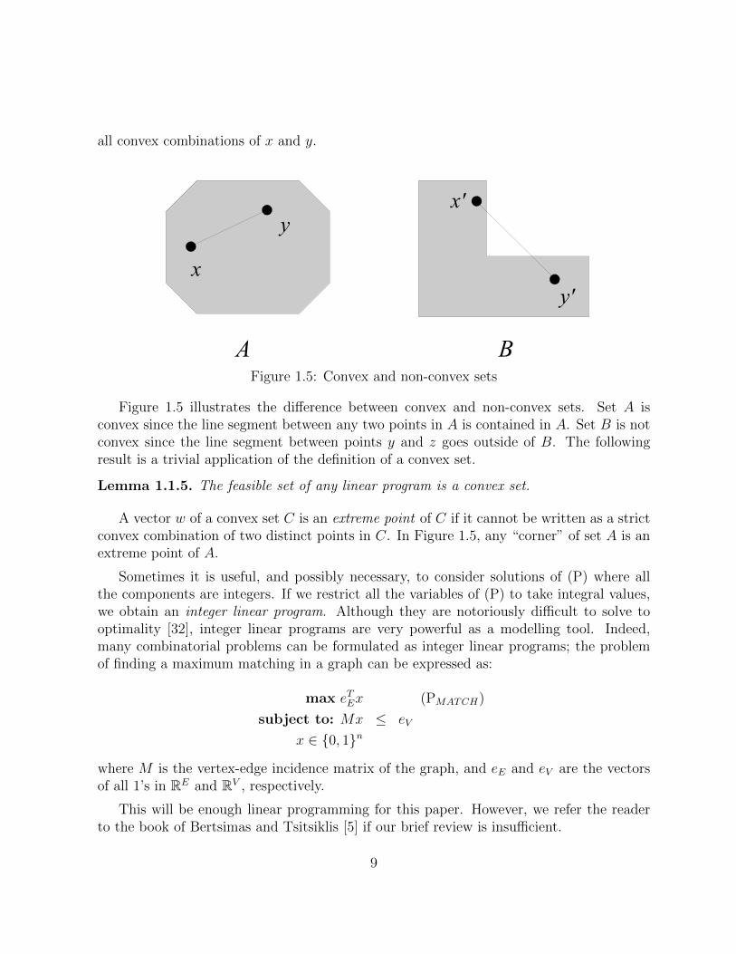
all convex combinations of x and y.

y

y'

x'

x

A BFigure 1.5: Convex and non-convex sets

Figure 1.5 illustrates the difference between convex and non-convex sets. Set A isconvex since the line segment between any two points in A is contained in A. Set B is notconvex since the line segment between points y and z goes outside of B. The followingresult is a trivial application of the definition of a convex set.

Lemma 1.1.5. The feasible set of any linear program is a convex set.

A vector w of a convex set C is an extreme point of C if it cannot be written as a strictconvex combination of two distinct points in C. In Figure 1.5, any “corner” of set A is anextreme point of A.

Sometimes it is useful, and possibly necessary, to consider solutions of (P) where allthe components are integers. If we restrict all the variables of (P) to take integral values,we obtain an integer linear program. Although they are notoriously difficult to solve tooptimality [32], integer linear programs are very powerful as a modelling tool. Indeed,many combinatorial problems can be formulated as integer linear programs; the problemof finding a maximum matching in a graph can be expressed as:

max eTEx (PMATCH)

subject to: Mx ≤ eV

x ∈ {0, 1}n

where M is the vertex-edge incidence matrix of the graph, and eE and eV are the vectorsof all 1’s in RE and RV , respectively.

This will be enough linear programming for this paper. However, we refer the readerto the book of Bertsimas and Tsitsiklis [5] if our brief review is insufficient.

9

1.1.3 Order Theory

A partially ordered set is a pair (P,�) where P is a set and � is a binary relation on theelements of P such that for all a, b, c ∈ P ,

• a � a,

• if a � b and b � a then a = b, and

• if a � b and b � c then a � c.

In other words, ‘�’ is a binary relation on P that is reflexive, transitive, and antisymmetric.Further, we will use a ≺ b to represent that a � b and a 6= b. For brevity we will say (P,�)is a poset or partial order. For example, let a, b ∈ N and define a � b to mean that adivides b. Then (N,�) is a poset.

Let (P,�) be a poset. If a 6� b and b 6� a then a and b are incomparable. In (N,�), 2and 3 are incomparable. The converse of a poset (P,�) is the poset (P,�c) where a �c bif and only if b � a.

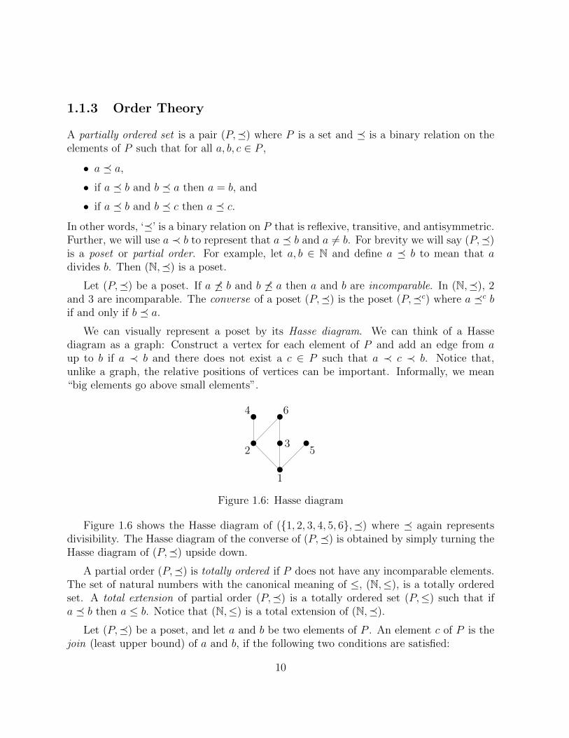
We can visually represent a poset by its Hasse diagram. We can think of a Hassediagram as a graph: Construct a vertex for each element of P and add an edge from aup to b if a ≺ b and there does not exist a c ∈ P such that a ≺ c ≺ b. Notice that,unlike a graph, the relative positions of vertices can be important. Informally, we mean“big elements go above small elements”.

1

23

4

5

6

Figure 1.6: Hasse diagram

Figure 1.6 shows the Hasse diagram of ({1, 2, 3, 4, 5, 6},�) where � again representsdivisibility. The Hasse diagram of the converse of (P,�) is obtained by simply turning theHasse diagram of (P,�) upside down.

A partial order (P,�) is totally ordered if P does not have any incomparable elements.The set of natural numbers with the canonical meaning of ≤, (N,≤), is a totally orderedset. A total extension of partial order (P,�) is a totally ordered set (P,≤) such that ifa � b then a ≤ b. Notice that (N,≤) is a total extension of (N,�).

Let (P,�) be a poset, and let a and b be two elements of P . An element c of P is thejoin (least upper bound) of a and b, if the following two conditions are satisfied:

10

• a ≤ c and b ≤ c, and

• for any w in P , such that a ≤ w and b ≤ w, we have c ≤ w.

We will denote such a c by a ∨ b. Analogously, we can define the meet of a and b, a ∧ b(greatest lower bound of a and b). If (P,�) is a poset and for every a, b ∈ P there existelements a ∨ b and a ∧ b in P then we say that (P,�) is a lattice.

A lattice is distributive if the following identities hold for every a, b, c ∈ P :

• a ∧ (b ∨ c) = (a ∧ b) ∨ (a ∧ c), and

• a ∨ (b ∧ c) = (a ∨ b) ∧ (a ∨ c).

These are often called the distributivity laws.

For our purposes, this is a sufficient introduction to order theory. However, additionalmaterial can be found in Gratzer’s book [17]. We are now ready to discuss stable match-ings.

11

Chapter 2

Stable Matchings in Graphs

Our examination of stable matchings begins with graphs. As we will see, our problemsfrom Chapter 1 can be modelled as matching problems in appropriate graphs. However, ourdefinition of a “graph” is incomplete for the purpose of studying stable matchings. Noticethat a major component of Problems 1, 2, and 3 is the set of preferences of the partiesinvolved. Intuitively, the set of stable matchings should depend on the set preferences.Indeed, this is the case. Therefore, we will be concerned with graphs that have additionalstructure.

Let G = (V,E) be a graph. For a vertex v, a preference list of v, Lv, is a totally orderedlist of the edges that contain v. If every vertex of G has a preference list we will say thatG = (V,E, L) is a graph with preferences where L is the set of vertex preference lists. Wewill take advantage of the fact that, in a graph, a vertex could rank either its incidentedges or its neighbour vertices; there is a one-to-one correspondence between the two sets.We will take the convention that a >v b means vertex v prefers edge a to edge b. We canalso replace the preference list of a vertex with a partially ordered set, called the preferenceposet. In this case G is a graph with poset preferences. Suppose Pv is the preference posetfor vertex v. If a and b are incomparable elements of Pv, then v considers a and b to beequally as good or tied.

Let G = (V,E, L) be a graph with preferences and let M be a matching of G. If there isan edge xy such that x and y prefer each other to their partners in the matching M , thenwe will call it a blocking edge for M . It is certainly possible that an endpoint of a blockingedge is unmatched in a matching. For our purposes, it will be convenient to imagine such avertex as being matched to itself. This will serve the noble purpose of reducing the numberof cases in many of our proofs. We will also say that the v-rank of an edge e is the positionof e in v’s preference list (i.e. v’s favourite edge has a v-rank of 1).

A matching M is a stable matching if for every edge xy 6∈ M either x prefers itspartner in M to y or y prefers its partner in M to x. Equivalently, we could define a

13

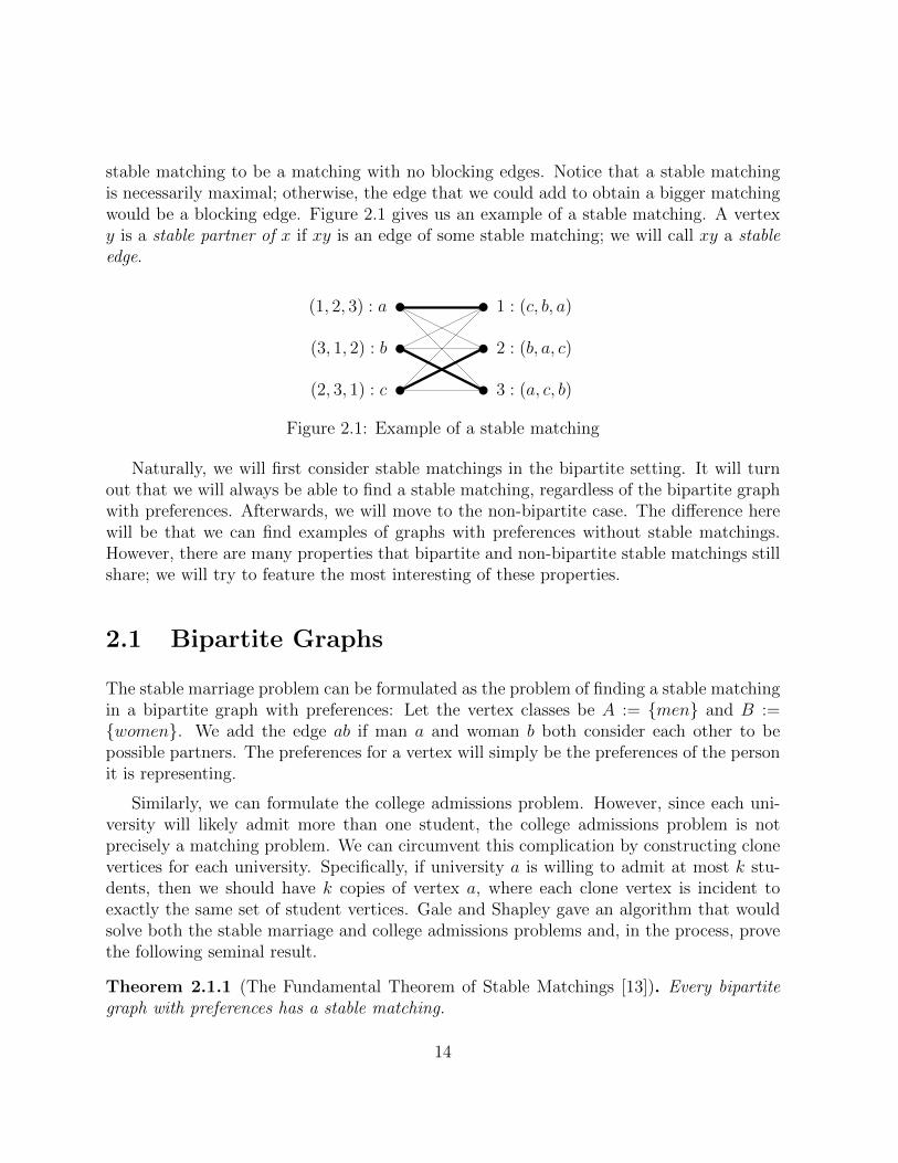
stable matching to be a matching with no blocking edges. Notice that a stable matchingis necessarily maximal; otherwise, the edge that we could add to obtain a bigger matchingwould be a blocking edge. Figure 2.1 gives us an example of a stable matching. A vertexy is a stable partner of x if xy is an edge of some stable matching; we will call xy a stableedge.

1 : (c, b, a)

2 : (b, a, c)

3 : (a, c, b)

(1, 2, 3) : a

(3, 1, 2) : b

(2, 3, 1) : c

Figure 2.1: Example of a stable matching

Naturally, we will first consider stable matchings in the bipartite setting. It will turnout that we will always be able to find a stable matching, regardless of the bipartite graphwith preferences. Afterwards, we will move to the non-bipartite case. The difference herewill be that we can find examples of graphs with preferences without stable matchings.However, there are many properties that bipartite and non-bipartite stable matchings stillshare; we will try to feature the most interesting of these properties.

2.1 Bipartite Graphs

The stable marriage problem can be formulated as the problem of finding a stable matchingin a bipartite graph with preferences: Let the vertex classes be A := {men} and B :={women}. We add the edge ab if man a and woman b both consider each other to bepossible partners. The preferences for a vertex will simply be the preferences of the personit is representing.

Similarly, we can formulate the college admissions problem. However, since each uni-versity will likely admit more than one student, the college admissions problem is notprecisely a matching problem. We can circumvent this complication by constructing clonevertices for each university. Specifically, if university a is willing to admit at most k stu-dents, then we should have k copies of vertex a, where each clone vertex is incident toexactly the same set of student vertices. Gale and Shapley gave an algorithm that wouldsolve both the stable marriage and college admissions problems and, in the process, provethe following seminal result.

Theorem 2.1.1 (The Fundamental Theorem of Stable Matchings [13]). Every bipartitegraph with preferences has a stable matching.

14

The ultimate goal of the next section will be to highlight this result and the Gale-Shapley algorithm. Later on we will also see that for a bipartite graph with preferences,the set of stable matchings forms a distributive lattice.

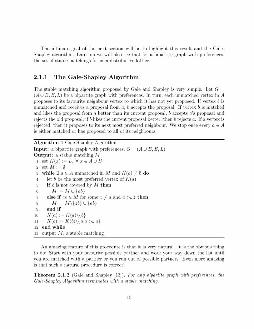
2.1.1 The Gale-Shapley Algorithm

The stable matching algorithm proposed by Gale and Shapley is very simple. Let G =(A ∪B,E,L) be a bipartite graph with preferences. In turn, each unmatched vertex in Aproposes to its favourite neighbour vertex to which it has not yet proposed. If vertex b isunmatched and receives a proposal from a, b accepts the proposal. If vertex b is matchedand likes the proposal from a better than its current proposal, b accepts a’s proposal andrejects the old proposal; if b likes the current proposal better, then b rejects a. If a vertex isrejected, then it proposes to its next most preferred neighbour. We stop once every a ∈ Ais either matched or has proposed to all of its neighbours.

Algorithm 1 Gale-Shapley Algorithm

Input: a bipartite graph with preferences, G = (A ∪B,E,L)Output: a stable matching M1: set K(x) := Lx ∀ x ∈ A ∪B2: set M := ∅3: while ∃ a ∈ A unmatched in M and K(a) 6= ∅ do4: let b be the most preferred vertex of K(a)5: if b is not covered by M then6: M := M ∪ {ab}7: else if zb ∈M for some z 6= a and a >b z then8: M := M\{zb} ∪ {ab}9: end if10: K(a) := K(a)\{b}11: K(b) := K(b)\{u|a >b u}12: end while13: output M , a stable matching

An amazing feature of this procedure is that it is very natural. It is the obvious thingto do: Start with your favourite possible partner and work your way down the list untilyou are matched with a partner or you run out of possible partners. Even more amazingis that such a natural procedure is correct!

Theorem 2.1.2 (Gale and Shapley [13]). For any bipartite graph with preferences, theGale-Shapley Algorithm terminates with a stable matching.

15

Proof: Let G = (A∪B,E,L) be a bipartite graph with preferences and let M∗ be the set ofedges returned by the algorithm. Lines 3 through 9 ensure that M∗ is indeed a matching.Suppose, for a contradiction, that M∗ is not stable. Then there exists a blocking edgeab ∈ E. Specifically, there exists a ∈ A and b ∈ B such that ab 6∈ M∗ and both a and bprefer each other to their partners (if they have one) in M∗.

Since ab 6∈ M∗ then either there exists z ∈ A who proposed to b during the algorithmsuch that z >b a or b never received a proposal throughout the algorithm. Notice that if breceives a proposal, then b is guaranteed to be matched at the end of the algorithm and willonly accept a new proposal if it is better than the current one. Therefore, if b receives aproposal, b is matched to a vertex w such that w ≥b z >b a, contradicting our assumptionthat ab is a blocking edge for M∗. If b did not receive a proposal then every vertex in A ismatched to a vertex in B that it prefers to b, again contradicting our assumption.

Observe that in order for the algorithm to always output a stable matching, any bi-partite graph with preferences must have a stable matching. In this way, Theorem 2.1.1follows directly from the algorithm.

Returning to our University of Waterloo Career Services example from Chapter 1, areasonable conjecture is that the algorithm used to match students to employers is a variantof the above algorithm, with A = {employers} and B = {students}. Unfortunately,a quick search through the Career Services website shows that this conjecture is false.The algorithm used by the Co-operative Education program is “greedy” and does notguarantee a stable matching [50]. However, it is noteworthy that, ten years before the theGale-Shapley paper was published, the NRMP began using the Gale-Shapley algorithm tomatch newly graduated doctors with hospitals [41]. The NRMP has proven so successfulthat the program continues to use a version of the algorithm and thousands of hospitalsand doctors participate in the program [38].

We will refer the reader to the books of Knuth [33], or Gusfield and Irving [19], fora simple analysis of this algorithm. However, if the reader is not interested, we will justmention that the analysis essentially boils down to the fact that each vertex will proposeto each of its neighbours at most once. If there are n vertices then each vertex has at mostn− 1 neighbours; this gives us O(n2) as the running time.

The Gale-Shapley algorithm leads to some interesting theoretical consequences. Wewill mention two of these here. However, we will save the proofs of these results untilSection 2.3.

Theorem 2.1.3 (Gale and Sotomayor [14], McVitie and Wilson [35]). Let G be a bipartitegraph with preferences. If vertex v is unmatched in a particular stable matching of G, thenv is unmatched in all stable matchings of G.

Corollary 2.1.4. Let G be a bipartite graph with preferences. All stable matchings of Ghave the same size.

16

In anticipation of the underlying structure of stable matchings, we will call a stablematching A-optimal if every vertex in A is matched to the most preferred partner it canhave in any stable matching. Notice that in a bipartite graph with preferences, the A-optimal stable matching, should it exist, is unique. However, the existence of such a stablematching seems unlikely (the fact that it is a matching is surprising). Remarkably, Galeand Shapley showed that their algorithm could do more than just guarantee the existenceof a stable matching.

Lemma 2.1.5 (Gale and Shapley [13]). For any bipartite graph with preferences, the Gale-Shapley Algorithm terminates with the A-optimal stable matching.

Proof: Let M∗ be the stable matching given by the algorithm. Suppose, for a contra-diction, that M∗ is not the A-optimal stable matching. Then there exists another stablematching, M , and vertices a ∈ A and x, y ∈ B such that ax ∈ M∗, ay ∈ M , and y >a x.Since ay 6∈ M∗, y must have rejected a during the algorithm. This rejection must havehappened because y received a proposal from a vertex z ∈ A such that z >y a. Since pro-posals occur one at a time, we may assume that this is the first time during the algorithmthat a vertex in B rejected a proposal from a stable partner.

Now z cannot have a better stable partner than y since, at the time of z’s proposalto y, y was first on z’s preference list and ay was the first stable edge that was rejectedduring the algorithm. Thus, since zy 6∈M , z must prefer y to its partner in M . But thenzy is a blocking edge for M , contradicting that M is a stable matching.

We now know that the A-optimal stable matching exists. But, we actually know morethan that! The uniqueness of the A-optimal stable matching shows that the Gale-Shapleyalgorithm will always terminate with the same stable matching. However, throughoutour discussion of Gale-Shapley, we did not specify a proposal order for the vertices inA. Surprisingly, this is not a mistake. Such an order is not necessary! In the proof ofLemma 2.1.5 there were no special assumptions about the execution of the algorithm thatproduced M∗. Hence the proposal order is irrelevant: ANY execution of the algorithm ona bipartite graph with preferences will yield the A-optimal stable matching. We will seethis non-determinism again when we look at Irving’s algorithm.

Many aspects of our world, especially athletics and politics, share a common trait: Thetriumph of one group of people usually comes at the expense of another group. This isalso true with stable matchings in bipartite graphs with preferences.

Corollary 2.1.6 (McVitie and Wilson [36]). In the A-optimal stable matching, each vertexin B is matched with the least preferred vertex it can have in any stable matching.

Proof: Let M∗ be the A-optimal stable matching and let M be another stable matching.Let a, w ∈ A, x, y ∈ B such that ay ∈ M∗, wy ∈ M , and ax ∈ M . Suppose, for a

17

contradiction, that a >y w. Since M∗ is the A-optimal stable matching and ay ∈ M∗, wemust have y >a x. Then ay is a blocking edge for M . But this contradicts that M is astable matching, since ay 6∈M .

This result justifies using the alternate term B-pessimal in place of A-optimal. Bythe noted anti-symmetry of the stable matching problem, we obtain the B-optimal/A-pessimal stable matching by simply running the algorithm with the women as the proposers.Further, the previous two results will give us maximal and minimal elements of the promisedlattice.

2.1.2 The Lattice of Stable Matchings

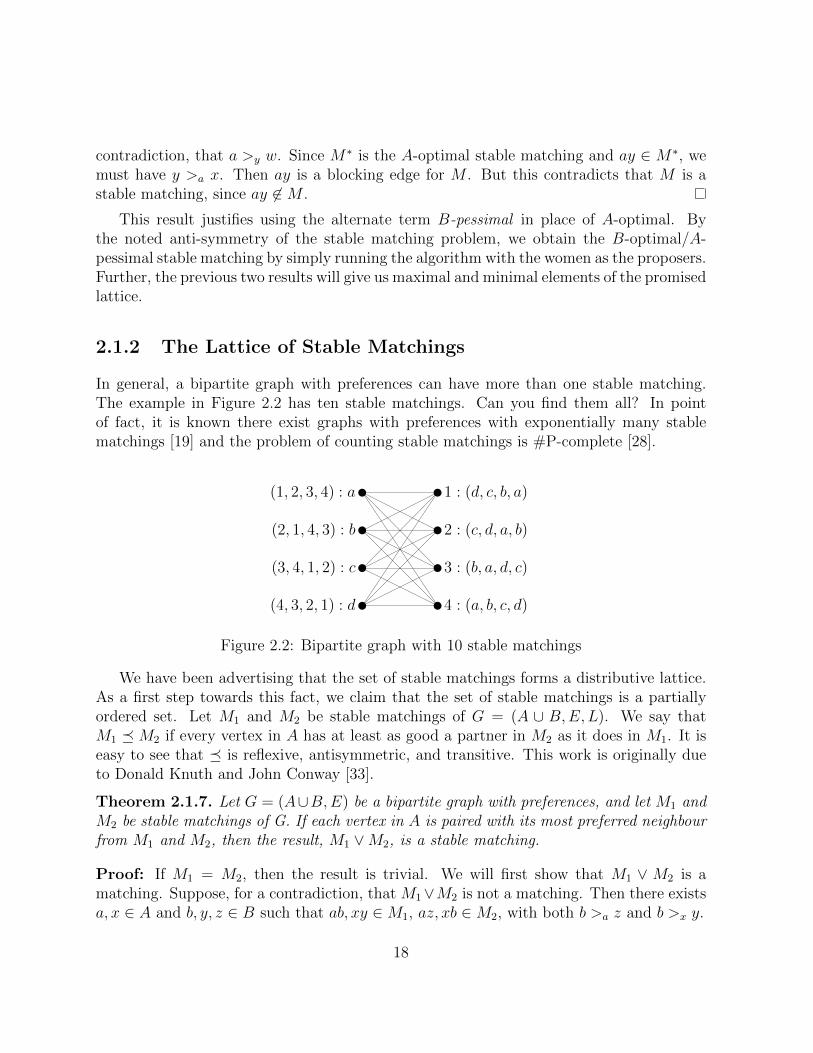
In general, a bipartite graph with preferences can have more than one stable matching.The example in Figure 2.2 has ten stable matchings. Can you find them all? In pointof fact, it is known there exist graphs with preferences with exponentially many stablematchings [19] and the problem of counting stable matchings is #P-complete [28].

1 : (d, c, b, a)

2 : (c, d, a, b)

3 : (b, a, d, c)

4 : (a, b, c, d)

(1, 2, 3, 4) : a

(2, 1, 4, 3) : b

(3, 4, 1, 2) : c

(4, 3, 2, 1) : d

Figure 2.2: Bipartite graph with 10 stable matchings

We have been advertising that the set of stable matchings forms a distributive lattice.As a first step towards this fact, we claim that the set of stable matchings is a partiallyordered set. Let M1 and M2 be stable matchings of G = (A ∪ B,E,L). We say thatM1 � M2 if every vertex in A has at least as good a partner in M2 as it does in M1. It iseasy to see that � is reflexive, antisymmetric, and transitive. This work is originally dueto Donald Knuth and John Conway [33].

Theorem 2.1.7. Let G = (A∪B,E) be a bipartite graph with preferences, and let M1 andM2 be stable matchings of G. If each vertex in A is paired with its most preferred neighbourfrom M1 and M2, then the result, M1 ∨M2, is a stable matching.

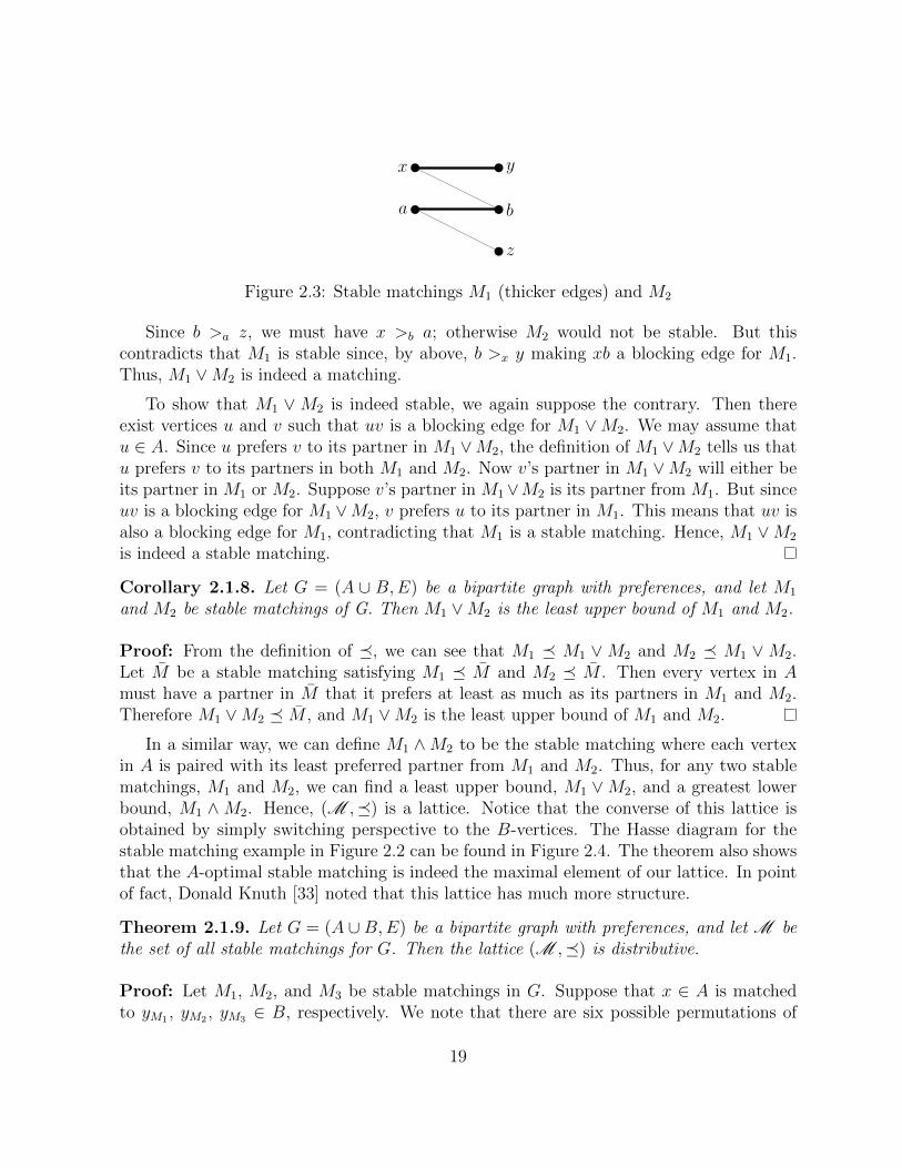
Proof: If M1 = M2, then the result is trivial. We will first show that M1 ∨ M2 is amatching. Suppose, for a contradiction, that M1∨M2 is not a matching. Then there existsa, x ∈ A and b, y, z ∈ B such that ab, xy ∈M1, az, xb ∈M2, with both b >a z and b >x y.

18

y

b

z

x

a

Figure 2.3: Stable matchings M1 (thicker edges) and M2

Since b >a z, we must have x >b a; otherwise M2 would not be stable. But thiscontradicts that M1 is stable since, by above, b >x y making xb a blocking edge for M1.Thus, M1 ∨M2 is indeed a matching.

To show that M1 ∨M2 is indeed stable, we again suppose the contrary. Then thereexist vertices u and v such that uv is a blocking edge for M1 ∨M2. We may assume thatu ∈ A. Since u prefers v to its partner in M1 ∨M2, the definition of M1 ∨M2 tells us thatu prefers v to its partners in both M1 and M2. Now v’s partner in M1 ∨M2 will either beits partner in M1 or M2. Suppose v’s partner in M1∨M2 is its partner from M1. But sinceuv is a blocking edge for M1 ∨M2, v prefers u to its partner in M1. This means that uv isalso a blocking edge for M1, contradicting that M1 is a stable matching. Hence, M1 ∨M2

is indeed a stable matching.

Corollary 2.1.8. Let G = (A ∪ B,E) be a bipartite graph with preferences, and let M1

and M2 be stable matchings of G. Then M1 ∨M2 is the least upper bound of M1 and M2.

Proof: From the definition of �, we can see that M1 � M1 ∨M2 and M2 � M1 ∨M2.Let M be a stable matching satisfying M1 � M and M2 � M . Then every vertex in Amust have a partner in M that it prefers at least as much as its partners in M1 and M2.Therefore M1 ∨M2 � M , and M1 ∨M2 is the least upper bound of M1 and M2.

In a similar way, we can define M1 ∧M2 to be the stable matching where each vertexin A is paired with its least preferred partner from M1 and M2. Thus, for any two stablematchings, M1 and M2, we can find a least upper bound, M1 ∨M2, and a greatest lowerbound, M1 ∧M2. Hence, (M ,�) is a lattice. Notice that the converse of this lattice isobtained by simply switching perspective to the B-vertices. The Hasse diagram for thestable matching example in Figure 2.2 can be found in Figure 2.4. The theorem also showsthat the A-optimal stable matching is indeed the maximal element of our lattice. In pointof fact, Donald Knuth [33] noted that this lattice has much more structure.

Theorem 2.1.9. Let G = (A ∪ B,E) be a bipartite graph with preferences, and let M bethe set of all stable matchings for G. Then the lattice (M ,�) is distributive.

Proof: Let M1, M2, and M3 be stable matchings in G. Suppose that x ∈ A is matchedto yM1 , yM2 , yM3 ∈ B, respectively. We note that there are six possible permutations of

19

yM1 , yM2 , and yM3 in the preference list for x. A simple calculation for each case yieldsM1 ∧ (M2 ∨M3) = (M1 ∧M2)∨ (M1 ∧M3) and M1 ∨ (M2 ∧M3) = (M1 ∨M2)∧ (M1 ∨M3),which are exactly the distributive laws.

There is much more substantial research into stable matching lattice theory [7, 19, 18,25, 28]. A particularly interesting result, motivated by a question of Knuth [33], showshow strong the connection is between stable matchings and lattice theory.

Theorem 2.1.10 (Blair [7]). Every finite distributive lattice is the lattice of stable match-ings for some bipartite graph with preferences.

Blair’s construction took a lattice on n points and gave a bipartite graph with prefer-ences with O(2n) vertices. Gusfield, Irving, Leather, and Saks [18] provided an efficientconstruction of the stable matching instance, while improving the size of the graph toO(n2).

Our detour through lattice theory may, admittedly, feel a little out of place here. How-ever, these remarkable and, in some sense, fairly simple, facts deserve inclusion in ourdiscussion.

a1, b2, c3, d4

a2, b1, c3, d4 a1, b2, c4, d3

a2, b1, c4, d3

a2, b4, c1, d3 a3, b1, c4, d2

a3, b4, c1, d2

a4, b3, c1, d2 a3, b4, c2, d1

a4, b3, c2, d1

Figure 2.4: Hasse diagram of stable matchings

2.2 Non-Bipartite Graphs

We begin our section on non-bipartite graphs with an example to highlight the mainobstacle when considering stable matchings in non-bipartite graphs with preferences. In

20

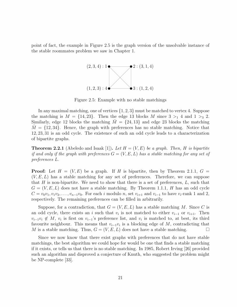
point of fact, the example in Figure 2.5 is the graph version of the unsolvable instance ofthe stable roommates problem we saw in Chapter 1.

2 : (3, 1, 4)

3 : (1, 2, 4)

(2, 3, 4) : 1

(1, 2, 3) : 4

Figure 2.5: Example with no stable matchings

In any maximal matching, one of vertices {1, 2, 3}must be matched to vertex 4. Supposethe matching is M = {14, 23}. Then the edge 13 blocks M since 3 >1 4 and 1 >3 2.Similarly, edge 12 blocks the matching M = {24, 13} and edge 23 blocks the matchingM = {12, 34}. Hence, the graph with preferences has no stable matching. Notice that12, 23, 31 is an odd cycle. The existence of such an odd cycle leads to a characterizationof bipartite graphs.

Theorem 2.2.1 (Abeledo and Isaak [1]). Let H = (V,E) be a graph. Then, H is bipartiteif and only if the graph with preferences G = (V,E, L) has a stable matching for any set ofpreferences L.

Proof: Let H = (V,E) be a graph. If H is bipartite, then by Theorem 2.1.1, G =(V,E, L) has a stable matching for any set of preferences. Therefore, we can supposethat H is non-bipartite. We need to show that there is a set of preferences, L, such thatG = (V,E, L) does not have a stable matching. By Theorem 1.1.1, H has an odd cycleC = v0v1, v1v2, . . . , vn−1v0. For each i modulo n, set vi+1 and vi−1 to have vi-rank 1 and 2,respectively. The remaining preferences can be filled in arbitrarily.

Suppose, for a contradiction, that G = (V,E, L) has a stable matching M . Since C isan odd cycle, there exists an i such that vi is not matched to either vi−1 or vi+1. Thenvi−1vi 6∈ M , vi is first on vi−1’s preference list, and vi is matched to, at best, its thirdfavourite neighbour. This means that vi−1vi is a blocking edge of M , contradicting thatM is a stable matching. Thus, G = (V,E, L) does not have a stable matching.

Since we now know that there exist graphs with preferences that do not have stablematchings, the best algorithm we could hope for would be one that finds a stable matchingif it exists, or tells us that there is no stable matching. In 1985, Robert Irving [26] providedsuch an algorithm and disproved a conjecture of Knuth, who suggested the problem mightbe NP-complete [33].

21

2.2.1 Irving’s Algorithm

Irving’s algorithm is divided into two phases. The first is very similar to the Gale-Shapleyalgorithm and removes edges that could not possibly be part of any stable matching. Themain difference here is that vertices can both give and receive proposals. The second phaseproceeds by deleting edges in a more specialized way until either we are left with a stablematching or we reach a condition that tells us that there is no stable matching.

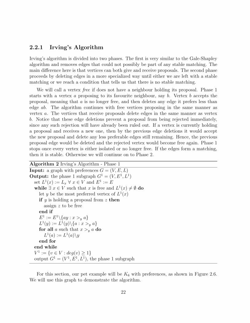
We will call a vertex free if does not have a neighbour holding its proposal. Phase 1starts with a vertex a proposing to its favourite neighbour, say b. Vertex b accepts theproposal, meaning that a is no longer free, and then deletes any edge it prefers less thanedge ab. The algorithm continues with free vertices proposing in the same manner asvertex a. The vertices that receive proposals delete edges in the same manner as vertexb. Notice that these edge deletions prevent a proposal from being rejected immediately,since any such rejection will have already been ruled out. If a vertex is currently holdinga proposal and receives a new one, then by the previous edge deletions it would acceptthe new proposal and delete any less preferable edges still remaining. Hence, the previousproposal edge would be deleted and the rejected vertex would become free again. Phase 1stops once every vertex is either isolated or no longer free. If the edges form a matching,then it is stable. Otherwise we will continue on to Phase 2.

Algorithm 2 Irving’s Algorithm - Phase 1

Input: a graph with preferences G = (V,E, L)Output: the phase 1 subgraph G1 = (V,E1, L1)

set L1(x) := Lx ∀ x ∈ V and E1 := Ewhile ∃ x ∈ V such that x is free and L1(x) 6= ∅ do

let y be the most preferred vertex of L1(x)if y is holding a proposal from z then

assign z to be freeend ifE1 := E1\{ay : x >y a}L1(y) := L1(y)\{a : x >y a}for all a such that x >y a doL1(a) := L1(a)\y

end forend whileV 1 := {v ∈ V : deg(v) ≥ 1}output G1 = (V 1, E1, L1), the phase 1 subgraph

For this section, our pet example will be K6 with preferences, as shown in Figure 2.6.We will use this graph to demonstrate the algorithm.

22

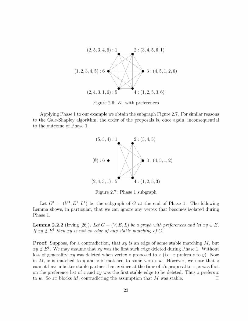
(2, 5, 3, 4, 6) : 1 2 : (3, 4, 5, 6, 1)

3 : (4, 5, 1, 2, 6)

4 : (1, 2, 5, 3, 6)(2, 4, 3, 1, 6) : 5

(1, 2, 3, 4, 5) : 6

Figure 2.6: K6 with preferences

Applying Phase 1 to our example we obtain the subgraph Figure 2.7. For similar reasonsto the Gale-Shapley algorithm, the order of the proposals is, once again, inconsequentialto the outcome of Phase 1.

(5, 3, 4) : 1 2 : (3, 4, 5)

3 : (4, 5, 1, 2)

4 : (1, 2, 5, 3)(2, 4, 3, 1) : 5

(∅) : 6

Figure 2.7: Phase 1 subgraph

Let G1 = (V 1, E1, L1) be the subgraph of G at the end of Phase 1. The followingLemma shows, in particular, that we can ignore any vertex that becomes isolated duringPhase 1.

Lemma 2.2.2 (Irving [26]). Let G = (V,E, L) be a graph with preferences and let xy ∈ E.If xy 6∈ E1 then xy is not an edge of any stable matching of G.

Proof: Suppose, for a contradiction, that xy is an edge of some stable matching M , butxy 6∈ E1. We may assume that xy was the first such edge deleted during Phase 1. Withoutloss of generality, xy was deleted when vertex z proposed to x (i.e. x prefers z to y). Nowin M , x is matched to y and z is matched to some vertex w. However, we note that zcannot have a better stable partner than x since at the time of z’s proposal to x, x was firston the preference list of z and xy was the first stable edge to be deleted. Thus z prefers xto w. So zx blocks M , contradicting the assumption that M was stable.

23

If we are lucky and Phase 1 ends with a matching, it would be nonsensical to suggestthat we need to do more work to reach a stable matching.

Lemma 2.2.3 (Irving [26]). If every vertex in G1 is adjacent to at most one other vertexthen the set of edges E1 form a stable matching in G.

The proof is similar to the proof that the Gale-Shapley algorithm is correct and istherefore omitted. To make our lives easier for the remainder of this section, we will relyheavily on the following two properties.

Property 1. Vertex a is in the current preference list of vertex b if and only if b is in thecurrent preference list of a.

Property 2. Vertex a is first in the current preference list of vertex b if and only if b islast in the current preference list of a.

Property 1 simply means that if we delete an edge ab, we must remember to remove bfrom a’s preference list and remove a from b’s preference list. Notice that Property 2 alsoholds in the Phase 1 subgraph, G1: Suppose vertex b receives a proposal from a. The factthat a proposed to b tells us that b was first in a’s preference list, otherwise a would haveproposed to a vertex it preferred more than b. Vertex a becomes last in b’s preference listbecause b deletes all of its neighbours it prefers less than a [26]. We will show that thesetwo properties hold throughout the algorithm, and will be essential to the proof that thealgorithm is correct.

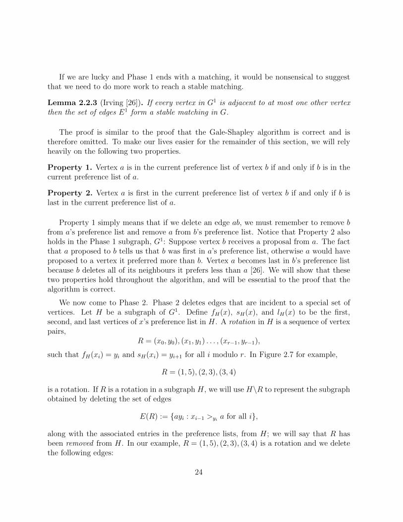
We now come to Phase 2. Phase 2 deletes edges that are incident to a special set ofvertices. Let H be a subgraph of G1. Define fH(x), sH(x), and lH(x) to be the first,second, and last vertices of x’s preference list in H. A rotation in H is a sequence of vertexpairs,

R = (x0, y0), (x1, y1) . . . , (xr−1, yr−1),

such that fH(xi) = yi and sH(xi) = yi+1 for all i modulo r. In Figure 2.7 for example,

R = (1, 5), (2, 3), (3, 4)

is a rotation. If R is a rotation in a subgraph H, we will use H\R to represent the subgraphobtained by deleting the set of edges

E(R) := {ayi : xi−1 >yi a for all i},

along with the associated entries in the preference lists, from H; we will say that R hasbeen removed from H. In our example, R = (1, 5), (2, 3), (3, 4) is a rotation and we deletethe following edges:

24

• 15 since 3 >5 1,

• 23 since 1 >3 2, and

• 34 and 45 since 2 >4 5 and 2 >4 3.

(3, 4) : 1 2 : (4, 5)

3 : (5, 1)

4 : (1, 2)(2, 3) : 5

(∅) : 6

Figure 2.8: Removing a rotation

Figure 2.8 shows the result of removing R. Since we are only deleting edges, the factthat Property 1 holds throughout Phase 2 is obvious. Property 2 also holds in Phase 2:Let H be a subgraph of G1 in which Properties 1 and 2 hold and let

R = (x0, y0), (x1, y1) . . . , (xr−1, yr−1)

be a rotation in H. When we remove R, we delete the edges E(R). In particular, we deleteall the edges of the form xiyi because xi is last in yi’s preference list. Notice also that wedo NOT delete edges of the form xi−1yi. Therefore, yi is now first in xi−1’s preference list.By definition of E(R), xi−1 is now also last in yi’s preference list. Deleting edges not ofthe form xiyi does not affect Property 2, since they are not first nor last in any preferencelist of H. So, Property 2 still holds in H\R, and rotation removal is well defined.

Lemma 2.2.4 (Irving [26]). Let H be a Phase 2 subgraph of G1. If H has a vertex withat least two neighbours then H has a rotation.

Proof: We first note that if vertex a has only one neighbour, say b, then by Properties 1and 2 the only neighbour of b is a. Let T be the set of vertices with at least two neighbours.Let v ∈ T . By the above observation, every neighbour of v is also in T . So for every x ∈ T ,sH(x) and lH(sH(x)) exist and are in T . Furthermore, if lH(sH(x)) = x then, by Property2, we would have fH(x) = sH(x), which is a contradiction since each neighbour of x canonly appear once on x’s preference list. Therefore, lH(sH(x)) 6= x.

Let D be a directed graph with nodes T and for every x ∈ T an outward arc tolH(sH(x)). Since every node has out-degree 1, there exists a directed cycle C. Let C =

25

x0, x1, . . . , xr−1. Note that xi+1 = lH(sH(xi)) for all i modulo r. By Property 2 thismeans that sH(xi) = f(xi+1). Let yi = f(xi) for all i modulo r and we can see thatR = (x0, y0), (x1, y1) . . . , (xr−1, yr−1) is a rotation.

Phase 2 can be described in the following way: While no vertex of V 1 is isolated andthe remaining edges are not a matching, find a rotation, which must exist by Lemma 2.2.4,and remove it. If some some vertex becomes isolated then there is no stable matching.Otherwise the matching we are left with is stable.

Algorithm 3 Irving’s Algorithm - Phase 2

Input: a graph with preferences G = (V,E, L) and its phase 1 subgraph G1 = (V 1, E1, L1)Output: a stable matching M , or proof that there is no stable matching in G

let V ′ = {v ∈ V |degG1(v) ≥ 1}let H = G1

while ∃ v ∈ V (H) such that degH(v) ≥ 2 and 6 ∃ u ∈ V (H) such that degH(u) = 0 dofind a rotation R in HH := H\R

end whileif ∃ u ∈ V (H) such that degH(u) = 0 then

output that G has no stable matchingelse

output M := E(H), a stable matchingend if

The next two results show that if a graph with preferences has a stable matching, thenat every iteration there will be at least one stable matching in the current subgraph of G1.Unlike the Gale-Shapley algorithm, the stable matching found by Irving’s algorithm is notunique; different sequences of rotation removals lead to different stable matchings.

Lemma 2.2.5 (Gusfield and Irving [19]). Let H be a Phase 2 subgraph of G1 and let Mbe a stable matching of G which is contained in H. If

R = (x0, y0), (x1, y1) . . . , (xr−1, yr−1)

is a rotation in H and xiyi 6∈M for some i, then M is contained in H\R.

Proof: Since rotations are cyclic we may assume x0y0 6∈M . By the definition of a rotation,x0 is therefore matched in M to, at best, y1. This means that, since M is a stable matching,y1 must be matched to a vertex it prefers at least as much as x0; otherwise x0y1 would bea blocking edge for M . Notice that by Property 2, x1 is last in y1’s preference list in H. Inparticular, y1 prefers x0 to x1. Therefore, we also have x1y1 6∈M since, as we just noticed,

26

y1 must be matched to a vertex at least as good as x0. Repeating this argument, we seethat xiyi 6∈ M , xi is matched in M to, at best, yi+1, and yi is matched in M to, at worst,xi−1 for all i modulo r. But when we remove R, we only delete an edge if some yi prefersthat edge less than yixi−1. Thus, no edge of M is deleted when we remove R, showing thatM is contained in H\R.

Theorem 2.2.6 (Irving [26], Gusfield and Irving [19]). Let H be a subgraph of G1 in Phase2 and suppose that H contains a stable matching of G. If

R = (x0, y0), (x1, y1) . . . , (xr−1, yr−1)

is a rotation in H, then there is a stable matching contained in H\R.

Proof: Let M be a stable matching of G and let R = (x0, y0), (x1, y1) . . . , (xr−1, yr−1) bea rotation in H. If there is an i such that xiyi 6∈ M , then Lemma 2.2.5 tells us that M iscontained in H\R. Thus, we may assume that xiyi ∈M for all i modulo r.

We first claim that {x0, . . . , xr−1} ∩ {y0, . . . , yr−1} = ∅. Otherwise there are i and jsuch that xi = yj. Note that xiyi, xjyj ∈ M . But this can only happen if xj = yi as well.Using Properties 1 and 2, we can say that

fH(xi) = yi = xj = lH(yj) = lH(xi).

Since the first vertex on the preference list of xi is the same as the last, xi has only onevertex in its preference list, contradicting our assumption that xi was in the rotation R.

Now, let M ′ be the matching obtained from M by replacing the edges xiyi with xiyi+1

for all i modulo r. Since R is cyclic and {x0, . . . , xr−1} ∩ {y0, . . . , yr−1} = ∅, M ′ is indeeda matching. We also note that M ′ is contained in H\R, since fH\R(xi) = yi+1 for all i andonly edges containing yi for some i can possibly be deleted when we remove R.

To complete the proof, we need only show that M ′ is stable. Suppose, for a contra-diction, that the edge uv blocks M ′. Since M is a stable matching, uv cannot block M .Notice that only the xi’s and yi’s have different matching partners in M ′ and only the xi’sprefer their partner in M to their partner in M ′. So any blocking edge for M ′ must involvesome xj. Therefore, we may assume that u = xj for some j.

Claim: The blocking edge uv is an edge of H\R.

Proof of Claim: Suppose, for a contradiction, that uv is not an edge of H\R. Then uv wasdeleted when we removed R. Therefore v = yi for some i and yi prefers xi−1 = lH\R(yi) tou. But this contradicts the assumption that uv blocks M ′ since xi−1yi ∈M by assumption.

So uv ∈ H\R and, by above, u = xj for some j. By definition of M ′, u’s partner inM ′ is first on its preference list in H\R. Since uv ∈ H\R, u must prefer fH\R(u) to v,contradicting the assumption that uv blocks M ′.

27

The proof of Theorem 2.2.6 has a corollary. Specifically, this follows from the sectionof the proof where we show M ′ is a stable matching.

Corollary 2.2.7. If, when Irving’s algorithm terminates, every vertex of V 1 has degree 1,then the remaining edges are a stable matching of G.

Let us prove that Irving’s algorithm really works (finally!). Let G = (V,E, L) be agraph with preferences. Recall that V 1 is the set of non-isolated vertices after Phase 1.First, suppose that G does not have a stable matching. By Corollary 2.2.7, Phase 2 cannotterminate with a perfect matching of G1. Also, we continue to remove rotations while thereis still a vertex of V 1 of degree at least 2. Therefore, there must exist a vertex of V 1 whichbecame isolated during Phase 2 to cause the algorithm to stop.

Now suppose that G has a stable matching. Lemma 2.2.2 tells us that Phase 1 doesnot affect any stable matching of G. So, all the stable matchings of G survive to see Phase2. Now, we keep removing rotations as long as there is a vertex of V 1 with degree at least2. Since an isolated vertex of V 1 implies no stable matching, Phase 2 must terminate as aperfect matching of G1. Theorem 2.2.6 tells us that as long as we are removing rotations,there will always be a stable matching in the remaining subgraph. Therefore, the remainingedges must be a stable matching of G.

Thus, Irving’s algorithm correctly identifies whether a graph with preferences has astable matching and, if it does, provides one for us.

Before we move on, we will briefly describe the running time of Irving’s algorithm.Phase 1 runs in O(n2) time for the same reason that the running time of the Gale-Shapleyalgorithm is O(n2). In his original paper [26], Irving showed how to implement Phase 2 torun in O(n2) time. This gives us an overall time complexity of O(n2).

2.3 Consequences of Irving’s Algorithm

In practice, we can use Irving’s algorithm to decide if a graph with preferences has a stablematching. It is equally useful as a theoretical tool. We will start with a simple observation.

Lemma 2.3.1. Let G be a graph with preferences. If, at the end of Phase 1, vertex v hasan empty preference list then v is not matched in any stable matching of G.

This follows directly from Lemma 2.2.2. Vertex v is not incident to any edges in G1 sono edge incident to v in G can be in any stable matching.

Lemma 2.3.2. Let G be a graph with preferences. If, at the end of Phase 1, vertex v hasa nonempty preference list then v is matched in every stable matching of G.

28

Proof: Let v be a vertex of G that has a nonempty preference list at the end of Phase 1.We first note that v must be first in the preference list of some vertex, say u. Otherwise,by the Pigeonhole principle, there is a vertex z such that z is first in the preference lists ofboth w and y. But, by Property 2, both w and y would then be last in the preference listof z. This is a contradiction since all the preference lists are total orders.

Now if v is unmatched in some stable matching M , then vu blocks M since vu 6∈ Mand u, by Lemma 2.2.2, is matched to a vertex it prefers less than v. Thus, v must bematched in every stable matching.

The next result follows easily from the previous two lemmas and is the non-bipartiteversion of Theorem 2.1.3 in Section 2.1.

Theorem 2.3.3 (Gusfield and Irving). Let G be a graph with preferences. If vertex v isunmatched in a particular stable matching of G, then v is unmatched in all stable matchingsof G.

We now know there exists a partition of the vertices: Vertices that are always matched ina stable matching and vertices that are never matched. Less technically, it does not matterwhich set of stable marriages we choose, the same set of people will never be married(possibly for the best). Once we have this partition, the consequence is inescapable. Yet,the conclusion still startles many people when they first hear it.

Corollary 2.3.4. Let G be a graph with preferences. If G has a stable matching, then allstable matchings of G have the same size.

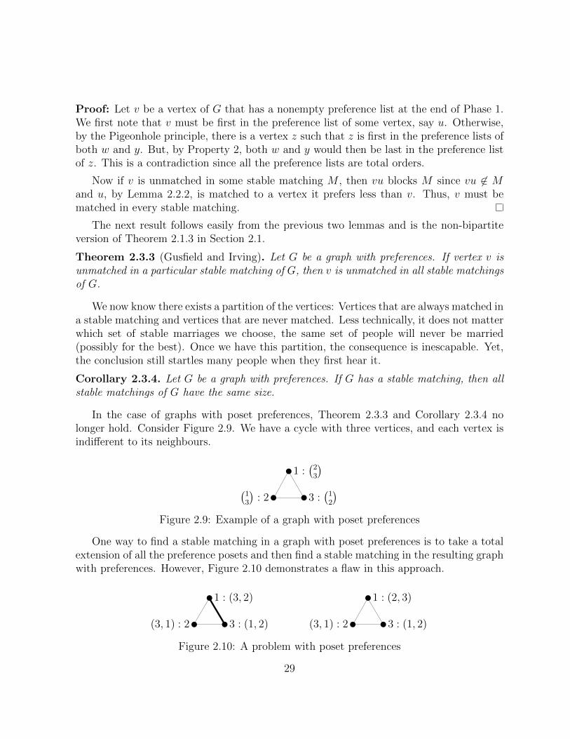
In the case of graphs with poset preferences, Theorem 2.3.3 and Corollary 2.3.4 nolonger hold. Consider Figure 2.9. We have a cycle with three vertices, and each vertex isindifferent to its neighbours.

1 :(23

)

3 :(12

)(13

): 2

Figure 2.9: Example of a graph with poset preferences

One way to find a stable matching in a graph with poset preferences is to take a totalextension of all the preference posets and then find a stable matching in the resulting graphwith preferences. However, Figure 2.10 demonstrates a flaw in this approach.

1 : (2, 3)

3 : (1, 2)(3, 1) : 2

1 : (3, 2)

3 : (1, 2)(3, 1) : 2

Figure 2.10: A problem with poset preferences

29

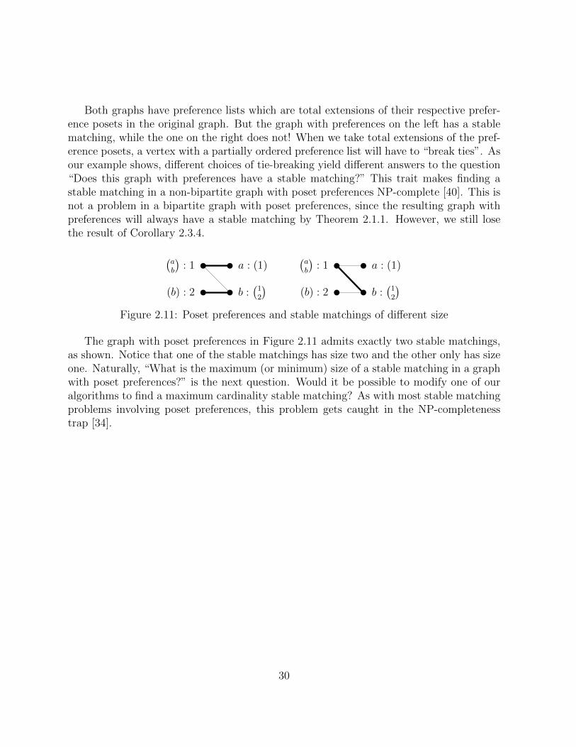
Both graphs have preference lists which are total extensions of their respective prefer-ence posets in the original graph. But the graph with preferences on the left has a stablematching, while the one on the right does not! When we take total extensions of the pref-erence posets, a vertex with a partially ordered preference list will have to “break ties”. Asour example shows, different choices of tie-breaking yield different answers to the question“Does this graph with preferences have a stable matching?” This trait makes finding astable matching in a non-bipartite graph with poset preferences NP-complete [40]. This isnot a problem in a bipartite graph with poset preferences, since the resulting graph withpreferences will always have a stable matching by Theorem 2.1.1. However, we still losethe result of Corollary 2.3.4.

(ab

): 1

(b) : 2

a : (1)

b :(12

)

(ab

): 1

(b) : 2

a : (1)

b :(12

)

Figure 2.11: Poset preferences and stable matchings of different size

The graph with poset preferences in Figure 2.11 admits exactly two stable matchings,as shown. Notice that one of the stable matchings has size two and the other only has sizeone. Naturally, “What is the maximum (or minimum) size of a stable matching in a graphwith poset preferences?” is the next question. Would it be possible to modify one of ouralgorithms to find a maximum cardinality stable matching? As with most stable matchingproblems involving poset preferences, this problem gets caught in the NP-completenesstrap [34].

30

Chapter 3

Fractional Stable Matchings

As we noted in Section 2.2, a non-bipartite graph may not have any stable matchings. Apossible way to avoid this unfortunate fact is to relax the “matching” requirement. Inthis chapter, we will be concerned with graphs with preferences. However, the preliminarydefinitions can be extended to hypergraphs with preferences and will be discussed in thiscontext later in Chapter 5.

A hypergraph with preferences, H = (V,E, L), is a hypergraph where every vertexhas a totally ordered list of its incident edges. Let H = (V,E, L) be a hypergraph withpreferences and let M be a matching of H. If there is an edge e ∈ E such that all thevertices of e prefer edge e to their respective edges of M , then we will call it a blockingedge for M . A matching, M , is stable if M does not have any blocking edges. In otherwords, if M is a stable matching for H, then for every e 6∈ M , at least one of the verticesof e prefers its matching edge to e.

A vector x ∈ RE+ is called a fractional matching if

∑

e∈E:u∈e

xe ≤ 1 for every u ∈ V.

A fractional matching x is called a fractional stable matching if every edge e contains avertex u such that ∑

e≤uj

xj = 1.

We will see that a hypergraph always admits a fractional stable matching regardless of thepreferences of the vertices. In some sense we can think of a fractional stable matching asa stable arrangement of timeshared partnerships: Suppose that i and j are the endpointsof edge e. The value of xe represents the proportion of time that i and j are roommates.

31

At least one of i and j will always have an additional situation that is preferred at least asmuch as the assignment of i to j. Admittedly, this is a curious metaphor since we describedthe original stable marriage problem as a way of preventing multiple partners. Fractionalstable matchings in graphs with preferences will eventually lead us to a structure calleda “stable partition”. Stable partitions very closely resemble stable matchings and can befound using a simple extension of Irving’s algorithm. In the process of our investigation wewill see necessary and sufficient conditions for the existence of stable matchings in graphswith preferences.

3.1 Scarf’s Lemma

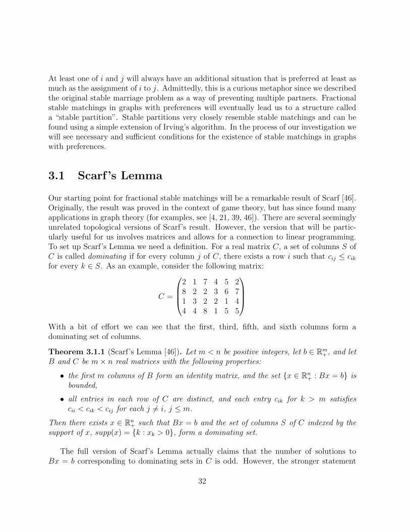
Our starting point for fractional stable matchings will be a remarkable result of Scarf [46].Originally, the result was proved in the context of game theory, but has since found manyapplications in graph theory (for examples, see [4, 21, 39, 46]). There are several seeminglyunrelated topological versions of Scarf’s result. However, the version that will be partic-ularly useful for us involves matrices and allows for a connection to linear programming.To set up Scarf’s Lemma we need a definition. For a real matrix C, a set of columns S ofC is called dominating if for every column j of C, there exists a row i such that cij ≤ cikfor every k ∈ S. As an example, consider the following matrix:

C =

2 1 7 4 5 28 2 2 3 6 71 3 2 2 1 44 4 8 1 5 5

With a bit of effort we can see that the first, third, fifth, and sixth columns form adominating set of columns.

Theorem 3.1.1 (Scarf’s Lemma [46]). Let m < n be positive integers, let b ∈ Rm+ , and let

B and C be m× n real matrices with the following properties:

• the first m columns of B form an identity matrix, and the set {x ∈ Rn+ : Bx = b} is

bounded,

• all entries in each row of C are distinct, and each entry cik for k > m satisfiescii < cik < cij for each j 6= i, j ≤ m.

Then there exists x ∈ Rn+ such that Bx = b and the set of columns S of C indexed by the

support of x, supp(x) = {k : xk > 0}, form a dominating set.

The full version of Scarf’s Lemma actually claims that the number of solutions toBx = b corresponding to dominating sets in C is odd. However, the stronger statement

32

requires additional assumptions on the matrices B and C. We will use Scarf’s Lemmato show the existence of a fractional stable matching in any hypergraph with preferences.Thus, the above version will be sufficient for our purposes. We refer the reader to thepapers of Haxell [21], Rioux [39], or Scarf [46] for a full treatment.

Let H = (V,E, L) be a hypergraph with preferences. The main obstacle that standsin the way of applying Scarf’s Lemma is the link between stability and a dominating setof columns. To that end we make the following definitions. Recall the definition of v-rankfrom the introduction to Chapter 2. Let v be a vertex, let e be an edge such that v ∈ e andlet i be e’s rank in the preference list of v. We define the value of e in the preference list of vto be deg(v)−i+1. For example, v’s favourite edge would have value deg(v)−1+1 = deg(v)and v’s least favourite edge would have value deg(v)− deg(v) + 1 = 1.

We need to encode the preferences of H into a matrix C. The rows of our matrix C willbe indexed by an arbitrary, but fixed, ordering of V . The columns will be indexed by V ∪E.The first |V | columns will be indexed by the same ordering as the rows. The remaining|E| columns will be indexed by some fixed ordering of E. Let v ∈ V . We first define all(v, e)-entries for e ∈ E: set the (v, e)-entry to be the value of e in the preference list of v ifv ∈ e, and otherwise we assign to {(v, e) : v 6∈ e} the values {deg(v) + 1, . . . , |E|} with anarbitrary permutation. Finally for the first |V | entries of row v we let the (v, v)-entry be0, and all other entries be distinct values strictly larger than |E|. We will call C the valuematrix of H.

Theorem 3.1.2 (Aharoni and Fleiner [4]). Every hypergraph with preferences has a frac-tional stable matching.

Proof: Let H = (V,E, L) be a hypergraph with preferences. Let C be the value matrix ofH and let B be the vertex-edge incidence matrix of H with the identity matrix appendedto its left. Both B and C have rows indexed by V and columns indexed by V ∪ E. Byconstruction, C satisfies the conditions of Theorem 3.1.1 and setting b as the all-1’s vectorallows B to meet the conditions of the theorem. Therefore, there exists x ∈ RV ∪E

+ satisfyingBx = b and a set of columns S, indexed by supp(x), which form a dominating set in matrixC. Let x ∈ RE

+ be the entries of x corresponding to the edges of H. We claim that x is afractional stable matching of H.

The definition of B and the fact that Bx = b ensures that x is a fractional matching.To check that x is fractionally stable, let h be an arbitrary edge. Then in the matrix Cthere exists a vertex v such that all entries in row v of the columns indexed by supp(x)are at least the (v, h)-entry. Note that the column v is not in supp(x) as the (v, v)-entryis strictly smaller than every other entry in row v. Therefore

∑e∈E:v∈e xe = 1. If v ∈ h,

then by the way we defined C, we see that every edge e for which v ∈ e and xe > 0 hasa higher value in the preference list of v than h. Therefore

∑h≤ve

xe = 1 as required. To

33

complete the proof we must show that the case where v 6∈ h cannot happen. Suppose, fora contradiction, that v 6∈ h. By the definition of C, the (v, h)-entry is at least deg(v) + 1.Thus, there is no edge e such that v ∈ e and xe > 0. Since Bx = b we must then havev ∈ supp(x), contradicting our earlier finding. Therefore x is a fractional stable matchingas required.

Interestingly, the existence of a fractional stable matching extends to hypergraphs withposet preferences.

Corollary 3.1.3. Every hypergraph with poset preferences has a fractional stable matching.

Proof: Let H = (V,E, P ) be a hypergraph with poset preferences. For all v ∈ V let Pv

be the preference poset of v and let Lv be a total extension of Pv. Consider the auxiliaryhypergraph with preferences H = (V,E, L) where L is the set of all Lv.

By Theorem 3.1.2, H has a fractional stable matching x. We claim that x is alsoa fractional stable matching for H. Clearly x is a fractional matching. Suppose, for acontradiction, that x is not a fractional stable matching for H. Then there exists an edgee such that

∑e≤vh

xh < 1 for all v ∈ e. In particular, for every v ∈ e there exists an edgef such that f <v e and xf > 0. Since f <v e in Pv, we must have f <v e in Lv since Lv

is a total extension of Pv. As x is a fractional matching,∑

e≤vhxh < 1 must hold in H as

well. This contradicts the assumption that x was a fractional stable matching for H.

3.2 Stable Partitions

Stable partitions were introduced by Tan [48] to provide a characterization of graphs withpreferences that have stable matchings. This characterization is known as Tan’s Theorem.Tan’s Theorem is similar in flavour to Tutte’s Theorem about perfect matchings and Ku-ratowski’s Theorem about planar graphs: The only impediment to a stable matching isa particular type of stable partition. We will prove this result later after we examine analgorithm to find stable partitions in a graph with preferences. In this section, we willintroduce stable partitions and their connection to fractional stable matchings.

A cycle C = {v0v1, v1v2, . . . , vn−2vn−1, vn−1v0} of a graph with preferences G = (V,E, L)is a preference cycle if vi−1vi <vi vivi+1 for all i modulo n.

1 : (2, 3)

3 : (1, 2)(3, 1) : 2

Figure 3.1: Example of a preference cycle

34

A stable partition of G = (V,E, L) is a set of edges, S ⊆ E, with the following proper-ties:

• Any component of S is either a cycle, a single edge, or an isolated vertex,

• each cycle component of S is a preference cycle, and

• for any e ∈ E\S, there is a vertex v, incident with an edge of S, such that v ∈ e ande <v f for any f ∈ S with v ∈ f .

Notice that if S does not contain any cycles, then S is actually a stable matching. Inthe case that S contains a preference cycle component of odd length, we will say that S isan odd stable partition.

Theorem 3.2.1 (Tan [48]). Every graph with preferences has a stable partition.

Proof: Let G = (V,E, L) be a graph with preferences. By Theorem 3.1.2 G has a fractionalstable matching x ∈ RE

+. Let S = supp(x). We will show that S is a stable partition. Sincex is a fractional stable matching, we can orient each edge e towards a vertex v such that∑

e≤vjxj = 1.

Claim 1: Each vertex v is the head of, at most, one arc in S.

Proof of Claim 1: Suppose vertex v is the head of arcs e, h ∈ S. Without loss of generality,we may assume that e <v h. Since v is the head of both arcs, we see that

∑e≤vj

xj = 1and

∑h≤vj

xj = 1. But since e <v h, we must have xe = 0, contradicting that e ∈ S.

Claim 2: If e, f is a directed path and e, f ∈ S, then there is a g ∈ S such that e, f, g is adirected path or a directed 3-cycle.

Proof of Claim 2: Let w ∈ V be the tail of f (head of e). Since e is oriented towards w wehave e <w f . Let z = head(f). Note that xf < 1 as x is a fractional matching. Since x isalso a fractional stable matching, there must be an edge g ∈ S such that tail(g) = z andf <z g. If head(g) = tail(e) then e, f, g is a directed 3-cycle. Otherwise e, f, g is a directedpath.

Claim 3: Each vertex v is the tail of, at most, one arc in S.

Proof of Claim 3: Suppose vertex v is the tail of arcs e, h ∈ S. Let z = head(e) andw = head(h). Note that xe and xh are both strictly less than 1. By Claim 1 and our choiceof edge orientations, there must exist arcs f, k ∈ S such that tail(f) = z and tail(k) = w.Repeatedly applying Claims 1 and 2 shows that there is a directed cycle C1 containing thepath e, f and another directed cycle C2 containing the path h, k. Note that all the arcs of

35

C1 and C2 are in S. Since C1 and C2 share vertex v, there must be a vertex that is thehead of two arcs of S, contradicting Claim 1.

Claims 1 and 3 imply that each vertex is incident to, at most, two edges of S. Claim2 implies that any path of length at least two is actually part of a cycle of edges of S.These two properties show that any component of G induced by S is either an isolatedvertex, a single edge or a cycle. Note that the proof of Claim 2 also implies that any cyclecomponent is a preference cycle.

Finally, let i ∈ E\S and suppose that i is oriented as ab. Note that xi = 0 and∑i≤bj

xj = 1. By definition of S and our choice of edge orientation, we must have i <b sfor all s such that b ∈ s and s ∈ S. Thus S is indeed a stable partition.

The proof presented here is due to Aharoni and Fleiner [4]. We will give another proof(similar to Tan’s proof) of this result in the next section when we examine Tan’s Algorithmand show that it will always find a stable partition.

A very nice consequence of the definition of stable partition and Theorem 3.2.1 is thatonce we have a stable partition, we automatically have a fractional stable matching. As wewill see, this fractional stable matching has a very nice property: xe ∈ {0, 1

2, 1} for every

e ∈ E. These special fractional stable matchings are called half-integral stable matchings.

Theorem 3.2.2 (Tan [48], Aharoni and Fleiner [4]). Every graph with preferences has ahalf-integral stable matching.

Proof: Let G = (V,E, L) be a graph with preferences. Theorem 3.2.1 ensures that G hasa stable partition S. Recall that the components of S are either cycles or edges. For everye ∈ E define

xe =

1 if e is an edge component of S12

if e is an edge of a cycle component of S

0 otherwise.

We claim that x is a half-integral stable matching. Note that x is certainly a fractionalmatching, while

∑e∈E:v∈e xe = 1 if v is incident to an edge of S and

∑e∈E:v∈e xe = 0

otherwise. First, let e 6∈ S. Since S is a stable partition, e has an endpoint v suchthat e <v f for every f ∈ S such that v ∈ f . If v is in an edge component of S, thenxf = 1, implying that

∑j∈E:e≤vj

xj = 1. If v is in a cycle component of S, then there are

g, h ∈ S incident with v such that e <v g and e <v h. Since xg = xh = 12, the result is∑

j∈E:e≤vjxj = 1.

Now, let e ∈ S. If e is in an edge component of S, then since x is a fractional matchingand xe = 1, we have

∑j∈E:e≤vj

xj = 1 for some endpoint, v, of e. If e is in a cyclecomponent, then since the cycle is a preference cycle, there exist a vertex u and an edge

36

f such that u ∈ e, u ∈ f and e <u f . Our definition of x ensures that∑

j∈E:e≤ujxj = 1.

Thus x is, indeed, a half-integral stable matching.

Notice that if a cycle component C has an even number of edges, we could insteaddefine the edge variables to alternate between 0 and 1 as we go around the cycle. Then wesee that the above proof is still valid. Thus, a stable partition with no odd cycles inducesa stable matching.

As with Corollary 3.1.3 in the previous section, consider a graph with poset preferences.Once again we can take a total extension of the preference poset for every vertex to obtaina half-integral stable matching in the auxiliary graph. Following the proof of Corollary3.1.3 yields the analogous result.

Corollary 3.2.3. Every graph with poset preferences has a half-integral stable matching.

3.2.1 Tan’s Algorithm

Given that a graph with preferences will always have a stable partition, it would be ideal tohave an algorithm to find such a set of edges. Tan gave such a procedure in 1991 [48]. Thealgorithm is essentially the same as Irving’s algorithm. In fact, Phase 1 is identical. Theonly difference will be our treatment of isolated vertices in Phase 2. Instead of stoppingwhen we find an isolated vertex, we will set aside the isolated vertices and continue thealgorithm on the non-isolated vertices. As a consequence, we will see that Tan’s algorithmprovides us with a characterization of graphs with preferences that do not have a stablematching.

We recommend that the reader be familiar with the definitions and results of Section2.2.1. For convenience, we will give a short review of how the Phase 1 algorithm works.Recall that a vertex x is “free” if there is no vertex z currently holding a proposal fromx. Free vertices propose to their favourite remaining neighbour until every vertex is eitherisolated or not free. If x proposes to vertex v, we delete all the edges incident to v that vprefers less than xv. Note that if v were holding a proposal from z then z would becomefree after x’s proposal to v because v deleted all the edges it preferred less than vz; so, wemust have x >v z in order for x to propose to y. Phase 1 continues as long as there is afree vertex x that is not isolated.

Exactly as in the case of stable matchings, the Phase 1 subgraph contains all stablepartitions.

Lemma 3.2.4 (Tan [48]). Let G = (V,E, L) be a graph with preferences and let xy ∈ E.If, at the end of Phase 1, xy 6∈ E1 then xy is not an edge of any stable partition of G.

37

Proof: Suppose, for a contradiction, that xy is an edge of some stable partition S, butxy 6∈ E1. We may assume that xy was the first such edge deleted during Phase 1. Withoutloss of generality, xy was deleted when vertex z proposed to x (i.e. z >x y). Now in S, x isincident to y and let w be the most preferred vertex adjacent to z. We note that z cannotbe incident to a better vertex in S than x since at the time of z’s proposal, x was first onthe preference list of z and xy was the first edge of S to be deleted. Thus x ≥z w.

If x >z w, then xz 6∈ S by definition of w. But this means that xz blocks S sincez >x y, contradicting that S is a stable partition. Otherwise, x = w. So degS(x) = 2 asxy, xz ∈ S. By definition of stable partition, the component containing the edges xy andxz is a preference cycle. So there must exist a vertex u, possibly y, such that zu ∈ S.However, w = x >z u and z >x y, contradicting that the component is a preference cycleand that S was a stable partition.

Algorithm 4 Tan’s Algorithm - Phase 1

Input: a graph with preferences G = (V,E, L)Output: the phase 1 subgraph G1 = (V 1, E1, L1)

set L1(x) := Lx ∀ x ∈ V and E1 := Ewhile ∃ x ∈ V such that x is free and L1(x) 6= ∅ do

let y be the most preferred vertex of L1(x)if y is holding a proposal from z then

assign z to be freeend ifE1 := E1\{ay : x >y a}L1(y) := L1(y)\{a : x >y a}for all a such that x >y a doL1(a) := L1(a)\y

end forend whileV 1 := {v ∈ V : deg(v) ≥ 1}output G1 = (V 1, E1, L1), the phase 1 subgraph

Once again we can ignore any isolated vertices at this point. By Lemma 3.2.4 thesevertices will be isolated in any stable partition. We now come to Phase 2 where we furtherdelete edges via removal of rotations.

Recall the definition of a “rotation” from Section 2.2.1 and that E(R) is the set ofedges that are deleted when we remove the rotation R. The essential ingredient in Tan’sAlgorithm is the observation that if a vertex becomes isolated after eliminating a rotationR, then E(R) can only be a very special set of edges.

38

Lemma 3.2.5 (Tan [47]). Let H be a subgraph of G1 in Phase 2 and let

R = (x0, y0), (x1, y1) . . . , (xr−1, yr−1)

be a rotation in H. If, after removing R from H, some vertex becomes isolated, then E(R)is exactly an odd preference cycle.

To prevent this thesis from being thrown across the room in frustration, we will omitthe extremely technical details of this result and refer the interested (and brave) readerto the papers of Tan [47, 48]. Nonetheless, here is a sketch of the proof: By definition ofrotation removal we can assume that x0 is an isolated vertex. We now make the observationthat to delete the edge x0y0, we must have y0 = xj and x0 = yj+1 for some j 6= 0. Then,using Properties 1 and 2 from Section 2.2.1, we can show that degH(xj) = 2. Finally, weapply induction to show that the same properties hold for all indices i modulo r and thatr is indeed odd. Hence, E(R) is an odd cycle. The fact that E(R) is a preference cyclefollows since R is a rotation.

As an illustration, consider the graph with preferences in Figure 2.6. Figure 2.8 showedthe state of the graph after Phase 1 and the removal of a rotation. Notice that

R = (1, 3), (2, 4), (3, 5), (4, 1), (5, 2)

is now a rotation and, if we remove it, the graph has no edges left. By inspection E(R) isan odd preference cycle.

During Phase 2 of Irving’s Algorithm, we stopped if we found an isolated vertex becausethere was no stable matching. Tan shows us that the absence of a stable matching impliesthe presence of an odd preference cycle. This preference cycle will turn out to be an oddcomponent of a stable partition.

We can describe Phase 2 in the following way: While there is an active vertex of degreeat least 2, Lemma 2.2.4 tells us that there is a rotation. Therefore, we find a rotation andremove it. If removing a rotation R causes a vertex to become isolated, add E(R) to Sand continue Phase 2 on the non-isolated vertices. If all remaining vertices have degree 1,add the remaining edges to S. Then, S will be a stable partition.

We are now ready to prove that Tan’s algorithm is indeed correct.

Theorem 3.2.6 (Tan [48]). For any graph with preferences, Tan’s algorithm outputs astable partition.

Proof: Let S be the set of edges given by Tan’s algorithm. Notice that, by Lemmas 3.2.4and 3.2.5, the edges of S form components which are either an isolated vertex, a singleedge, or a preference cycle. Thus, we need only show that S satisfies the third condition

39

of a stable partition. Suppose, for a contradiction, that S is not a stable partition. Thenthere exists an edge ab 6∈ S and edges aw, bz ∈ S such that b >a w and a >b z.

If ab was deleted during Phase 1, then without loss of generality, there is a vertex uthat proposed to vertex a such that u >a b. But this contradicts the fact that edge aw ∈ S,since if such a u existed, u >a b >a w which would have caused the edge aw to be deletedas well.

If ab was deleted during Phase 2, then as noted in the proof of Theorem 2.2.6, we mayassume that b = yi for some yi in the removed rotation

R = (x0, y0), (x1, y1) . . . , (xr−1, yr−1).

Since ab was deleted, we must have xi−1 >b a. By definition of rotation removal we alsosee that edge bz was deleted, since xi−1 >b a >b z. Again this contradicts our assumptionthat bz ∈ S. Thus S must be a stable partition.

Algorithm 5 Tan’s Algorithm - Phase 2

Input: a graph with preferences G = (V,E, L) and its phase 1 subgraph G1 = (V 1, E1, L1)Output: a stable partition S

let H := G1, and S = ∅while ∃ v ∈ V (H) such that degH(v) ≥ 2 do

find a rotation R in HJ := H\Rif ∃ u ∈ V (J) such that degJ(u) = 0 thenS := S ∪ E(R)V ′ := V (H)\{v ∈ V (H) : degJ(v) = 0}

end ifE ′ := E(H)\E(R) and L′ := L(H)\L(R)H := (V ′, E ′, L′)

end whileS := S ∪ E(H)output S, a stable partition

This procedure is almost identical to Irving’s Algorithm. The only difference comeswhen we find an isolated vertex in Phase 2. Instead of stopping, we store E(R) andcontinue removing rotations as if the algorithm did not find anything at all. So, it is nota surprising fact that the running time of Tan’s Algorithm remains O(n2) [48].

40

3.2.2 A Consequence of Tan’s Algorithm

Section 2.3 shows how many interesting properties of stable matchings in bipartite graphsactually extend to the non-bipartite case. This section will look at an implication of Tan’sAlgorithm and the existence of stable partitions. In particular, we will finally give a proofof Tan’s Theorem.

Theorem 3.2.7 (Tan’s Theorem [47]). A graph with preferences has a stable matching ifand only if it does not have an odd stable partition.

Given that all bipartite graphs with preferences have a stable matching, this resultshould not come as a huge surprise. As we saw in Theorem 1.1.1, any non-bipartite graphnecessarily has an odd cycle. Therefore, it is reasonable to suspect that the non-existenceof a stable matching in a graph with preferences must have something to do with an oddcycle. Tan’s Theorem simply confirms our suspicions.

The reader who is still awake at this point will realize that Tan’s characterization ofgraphs with preferences admitting stable matchings is missing only one piece.

Lemma 3.2.8 (Tan [48]). If G is a graph with preferences and has an odd stable partition,then G has no stable matching.

Proof: Suppose, for a contradiction, that G has an odd stable partition, S, and a stablematching M . Let A be the set of vertices who have a partner in M that they prefer morethan at least one of their neighbours in S. Let B be the set of vertices who have a partnerin M that they prefer less than all of their neighbours in S. Every vertex in A must bematched in M to a vertex in B. Otherwise, if ab ∈M , a ∈ A and b 6∈ B then both a and bwould prefer the edge ab to at least one of their partners in S which would contradict thatS is a stable partition. So we must have |A| ≤ |B|.

Now let xy ∈ S. If both x and y are in B, then both x and y prefer the edge xy totheir matching partners, contradicting that M is a stable matching. Let C be the verticesof a component of S. Since each component of S is either a single vertex, a single edge ora cycle, and no two adjacent edges are in B, we must have |A∩C| ≥ |B ∩C|. If C has anodd number of vertices then the inequality is strict. Let C be the set of components of S.

|A| =∑

C∈C

|A ∩ V (C)| >∑

C∈C

|B ∩ V (C)| = |B|.

The strict inequality comes from the fact that S is an odd stable partition and musttherefore have at least one odd component. Thus, we have a contradiction which gives usthe result.

41

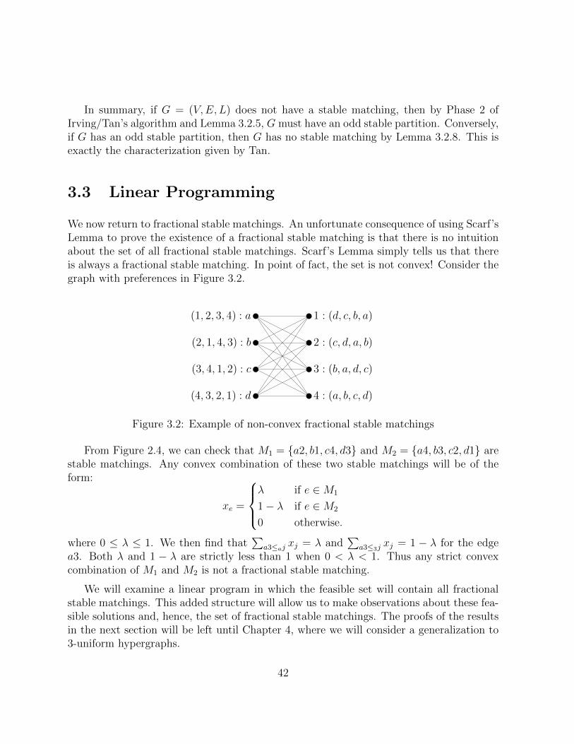
In summary, if G = (V,E, L) does not have a stable matching, then by Phase 2 ofIrving/Tan’s algorithm and Lemma 3.2.5, G must have an odd stable partition. Conversely,if G has an odd stable partition, then G has no stable matching by Lemma 3.2.8. This isexactly the characterization given by Tan.

3.3 Linear Programming

We now return to fractional stable matchings. An unfortunate consequence of using Scarf’sLemma to prove the existence of a fractional stable matching is that there is no intuitionabout the set of all fractional stable matchings. Scarf’s Lemma simply tells us that thereis always a fractional stable matching. In point of fact, the set is not convex! Consider thegraph with preferences in Figure 3.2.

1 : (d, c, b, a)

2 : (c, d, a, b)

3 : (b, a, d, c)

4 : (a, b, c, d)

(1, 2, 3, 4) : a

(2, 1, 4, 3) : b

(3, 4, 1, 2) : c

(4, 3, 2, 1) : d

Figure 3.2: Example of non-convex fractional stable matchings

From Figure 2.4, we can check that M1 = {a2, b1, c4, d3} and M2 = {a4, b3, c2, d1} arestable matchings. Any convex combination of these two stable matchings will be of theform:

xe =

λ if e ∈M1

1− λ if e ∈M2

0 otherwise.

where 0 ≤ λ ≤ 1. We then find that∑

a3≤ajxj = λ and

∑a3≤3j

xj = 1 − λ for the edgea3. Both λ and 1 − λ are strictly less than 1 when 0 < λ < 1. Thus any strict convexcombination of M1 and M2 is not a fractional stable matching.

We will examine a linear program in which the feasible set will contain all fractionalstable matchings. This added structure will allow us to make observations about these fea-sible solutions and, hence, the set of fractional stable matchings. The proofs of the resultsin the next section will be left until Chapter 4, where we will consider a generalization to3-uniform hypergraphs.

42

3.3.1 Stable Matchings and Linear Programming

The first linear programming formulation for stable matchings was given by Vande Vatein 1989 [51]. However, his formulation was only for stable matching problems where theunderlying graph was the complete bipartite graph, Km,n. Roth, Rothblum, and VandeVate [42] extended Vande Vate’s work to arbitrary bipartite graphs with preferences in1993. In 1994, Abeledo and Rothblum [3] showed that many interesting properties of thebipartite formulation easily extend to the non-bipartite case.

Recall that x ∈ RE+ is a fractional stable matching for a graph with preferences if it is a

fractional matching and for every edge ij either∑

a≥ijxia = 1, or

∑b≥ji

xjb = 1. Observethat any fractional stable matching is a feasible solution to the following linear program:

max∑

ij∈E

xij (PSM)

subject to:∑

j∈N(i)

xij ≤ 1 i ∈ V∑

a>ij

xia +∑

b>ji

xjb + xij ≥ 1 ij ∈ E

xij ≥ 0 ij ∈ E.

Suppose we take another look at the example in Figure 3.2. Notice that, since M1 andM2 are stable matchings, the vectors

xe =

{1 if e ∈M1

0 otherwise

and

xe =

{1 if e ∈M2

0 otherwise

are feasible for (PSM). Since the feasible region of any linear program is convex, any convexcombination of x and x is also a feasible solution to (PSM). But we showed that any strictconvex combination of x and x is not a fractional stable matching. Therefore, the feasiblesolutions of (PSM) are not necessarily fractional stable matchings. However, this does notmake (PSM) useless! Since we now know that every graph with preferences has a fractionalstable matching, Theorem 3.1.2 implies that the feasible set of (PSM) is always non-empty.As we will see, this linear program has some very useful properties which can be transferreddirectly to the set of fractional stable matchings.

43

Lemma 3.3.1 (Roth, Rothblum, and Vande Vate [42], Abeledo and Rothblum [3]). Let Gbe a graph with preferences. The incidence vectors of stable matchings of G are preciselythe feasible integer solutions to (PSM).

It is well known that integer programming is a hard problem in general [32]. A naturalquestion to ask is: Can we add any other constraints to (PSM) and obtain the convexhull of the incidence vectors of stable matchings? Or in other words: Is there a linearprogramming formulation for stable matchings such that the extreme points of the feasiblesolutions are exactly the stable matchings? Such a formulation would allow us to solveany linear optimization problem over the set of stable matchings using a suitable linearprogramming algorithm. Sadly, this is not the case.

Theorem 3.3.2 (Feder [11]). Let G be a graph with preferences. It is NP -hard to optimizea linear function over the set of stable matchings of G.

We should point out that Feder’s result does not mean that the extreme point solutionsto (PSM) can be arbitrary.

Theorem 3.3.3 (Abeledo and Rothblum [3]). Let G be a graph with preferences and letS be the set of feasible solutions to (PSM). Then the extreme points of S are half-integral.

By the above comments, an ideal formulation would have extreme points with integralcoordinates. It turns out (not surprisingly) that by restricting our focus to bipartite graphswith preferences, (PSM) is such a formulation.

Theorem 3.3.4 (Vande Vate [51], Rothblum [45]). Let G be a bipartite graph with pref-erence lists and let S be the set of feasible solutions to (PSM). Then the extreme points ofS are exactly the incidence vectors of stable matchings of G.

In the bipartite case, we now have that the feasible set of (PSM) is a non-empty poly-tope and its extreme points are always integral. This leads us to another proof of TheFundamental Theorem of Stable Matchings from Section 2.1.

As mentioned earlier, duality and complementary slackness play a leading role in thelinear programming perspective of stable matchings. Obviously we need a dual linearprogram to fully utilize these tools. The dual of (PSM) is the following:

min∑

i∈V

yi −∑

ij∈E

zij (DSM)

subject to: yi ≥ 0 i ∈ Vzij ≥ 0 ij ∈ E

yi + yj −∑

j>ia

zia −∑

i>jb

zjb − zij ≥ 1 ij ∈ E.

44

Although it is worthwhile to work through the details to obtain (DSM) (and wouldprobably be an excellent assignment question in a linear programming course), we willleave this as an exercise for the reader.

Lemma 3.3.5 (Abeledo and Rothblum [3]). Let x be a feasible solution to (PSM) and lety ∈ RV and z ∈ RE be defined as follows:

yi =∑

j∈N(i)

xij i ∈ V,

zij = xij ij ∈ E.Then (y, z) is a feasible solution to (DSM).

Theorem 3.3.6 (Roth, Rothblum, and Vande Vate [42], Abeledo and Rothblum [3]). Letx be a feasible solution to (PSM). Then x is also an optimal solution to (PSM).

It is also true that the (y, z) defined in Lemma 3.3.5 is optimal for (DSM). This willturn out to be very important when we look at the proofs of these results. The followingcorollary is now immediate.

Corollary 3.3.7. Let G be a graph with preferences. If G has a stable matching, then allstable matchings of G have the same size.

This is exactly the conclusion of Corollary 2.3.4. Additionally, Theorem 2.3.3 is a trivialconsequence of the following result.

Theorem 3.3.8 (Roth, Rothblum, and Vande Vate [42], Abeledo and Rothblum [3]). LetG = (V,E, L) be a graph with preferences. There exists a partition (A,B) of V such thatfor every feasible solution x to (PSM),

∑

j∈N(i)

xij = 1 if i ∈ A,

∑

j∈N(i)

xij = 0 if i ∈ B.

This partition of the vertices can even give us a sufficient condition for the non-existenceof a stable matching.

Corollary 3.3.9 (Abeledo and Rothblum [3]). Let G be a graph with preferences. If |A|is odd then G does not have a stable matching.

The main point here is that linear programming can provide alternate proofs to manyof the results in Chapter 2 without relying on the properties of an algorithm. Furthermore,these properties extend to the fractional case since fractional stable matchings are feasiblesolutions to (PSM). We will see this approach again, along with extensions of many of theproofs, in Section 4.2.

45

Chapter 4

3-Uniform Hypergraphs

Let us return to our time travelling adventure from Chapter 1. However, against the adviceof many science fiction enthusiasts, we are going to allow some small changes to the past.

First, suppose that your university has several options for residence and you decide youwould like to live in an apartment. This means that, instead of having a single roommate,you will have several roommates. We will assume that each apartment will have threeoccupants. The school is faced with essentially the same problem as before: Can it assignstudents to apartments so that there is no group of three students who would rather livetogether than with their assigned roommates?

The other change we will make comes when you get married: Your future spouse hasagreed to marry you only if you agree to having a dog. Now, instead of only finding a spouse,you have to worry about finding a spouse AND a dog. We will make the assumption thatthe dogs know what kinds of dog food they will be fed by each possible couple, so that theywill be able to rank their possible owners. Once again, the goal is to avoid man-woman-dogtriplets that prefer each other to their respective families.

Our motivational problems from Chapter 1 have the following hypergraphic cousins:

Problem 4 (Threesome Roommates Problem). Suppose there are n people living in auniversity dormitory. Each person ranks the other

(n−1

2

)pairs of students in terms of who

they would prefer to have as roommates. Can we find an assignment of roommates suchthat if three students are not roommates then at least one of them prefers their currentroommates?

Problem 5 (Stable Family Problem). A community consists of n men, n women, andn dogs. Each man ranks every woman-dog pair in terms of who they would prefer for afamily. Similar rankings are made by each woman and dog. Can we find a set of familiessuch that if a man, a woman, and a dog are not a family then at least one of them preferstheir current family?

47

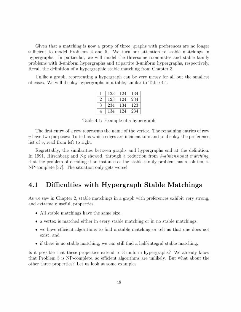
Given that a matching is now a group of three, graphs with preferences are no longersufficient to model Problems 4 and 5. We turn our attention to stable matchings inhypergraphs. In particular, we will model the threesome roommates and stable familyproblems with 3-uniform hypergraphs and tripartite 3-uniform hypergraphs, respectively.Recall the definition of a hypergraphic stable matching from Chapter 3.

Unlike a graph, representing a hypergraph can be very messy for all but the smallestof cases. We will display hypergraphs in a table, similar to Table 4.1.

1 123 124 1342 123 124 2343 234 134 1234 134 124 234

Table 4.1: Example of a hypergraph

The first entry of a row represents the name of the vertex. The remaining entries of rowv have two purposes: To tell us which edges are incident to v and to display the preferencelist of v, read from left to right.

Regrettably, the similarities between graphs and hypergraphs end at the definition.In 1991, Hirschberg and Ng showed, through a reduction from 3-dimensional matching,that the problem of deciding if an instance of the stable family problem has a solution isNP-complete [37]. The situation only gets worse!

4.1 Difficulties with Hypergraph Stable Matchings

As we saw in Chapter 2, stable matchings in a graph with preferences exhibit very strong,and extremely useful, properties:

• All stable matchings have the same size,

• a vertex is matched either in every stable matching or in no stable matchings,

• we have efficient algorithms to find a stable matching or tell us that one does notexist, and

• if there is no stable matching, we can still find a half-integral stable matching.

Is it possible that these properties extend to 3-uniform hypergraphs? We already knowthat Problem 5 is NP-complete, so efficient algorithms are unlikely. But what about theother three properties? Let us look at some examples.

48

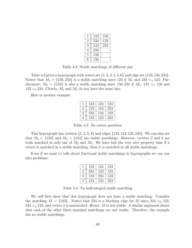
1 123 1562 234 1233 123 2344 2345 1566 156

Table 4.2: Stable matchings of different size

Table 4.2 gives a hypergraph with vertex set {1, 2, 3, 4, 5, 6} and edge set {123, 156, 234}.Notice that M1 = {156, 234} is a stable matching since 123 6∈ M1 and 234 >2 123. Fur-thermore, M2 = {123} is also a stable matching since 156, 234 6∈ M2, 123 >1 156 and123 >3 234. Clearly, M1 and M2 do not have the same size.

Here is another example:

1 123 124 1342 123 124 2343 234 134 1234 134 124 234

Table 4.3: No vertex partition

This hypergraph has vertices {1, 2, 3, 4} and edges {123, 124, 134, 234}. We can also seethat M3 = {123} and M4 = {134} are stable matchings. However, vertices 2 and 4 areboth matched in only one of M3 and M4: We have lost the very nice property that if avertex is matched in a stable matching, then it is matched in all stable matchings.

Even if we want to talk about fractional stable matchings in hypergraphs we can runinto problems:

1 123 124 1342 234 123 1243 134 234 1234 124 134 234

Table 4.4: No half-integral stable matching

We will first show that this hypergraph does not have a stable matching. Considerthe matching M = {123}. Notice that 234 is a blocking edge for M since 234 >2 123,234 >3 123, and vertex 4 is unmatched. Hence, M is not stable. A similar argument showsthat each of the other three maximal matchings are not stable. Therefore, the examplehas no stable matchings.

49

What can we say about its fractional stable matchings? Recall that a fractional match-ing x is called a fractional stable matching if every edge e contains a vertex u such that

∑

e≤uj

xj = 1.

A graph may or may not have a stable matching, but we know that it will always have afractional stable matching where every edge takes a value in the set {0, 1

2, 1}.

Suppose that this hypergraph has a half-integral stable matching. Since it does not havea stable matching, some edge must have a value of 1

2. The preference lists have a cyclic

structure, so we may assume that x123 = 12. The definition of a fractional stable matching

tells us that since x123 = 12, we must have either x234 = 1

2or x134 = 1

2. If the former is true,

then the same argument shows that either x134 = 12

or x124 = 12. Now, x134 6= 1

2since the

sum of the edges at vertex 3 would be 32

and not a matching. But, x124 6= 12

because vertex2 runs into the same problem. Thus, it is not possible to have x234 = 1

2. The x134 = 1

2case

is very similar and is left to the reader. There is no half-integral stable matching. In fact,the best fractional stable matching can be found by giving each edge a value of 1

3.

The point of these examples is this: All of our properties can fail to exist when wemove to hypergraphs! We must hope there is a special case of stable matchings that willyield these properties.

4.2 Majority Stable Matchings

Let H be a 3-uniform hypergraph with preferences and let M be a matching of H. Recallthat M is a stable matching if for every edge ijk 6∈ M , at least one of i,j, or k prefers itsmatching edge to ijk. If every ijk 6∈ M has the stronger property that at least TWO ofi, j, and k prefer their matching edge to ijk, then we will say that M is a majority stablematching. Once more, we can alternatively define a majority stable matching in terms ofblocking edges. In this case, a blocking edge for a matching M is an edge ijk 6∈ M suchthat at least two of i, j, and k prefer the edge ijk to their respective matching edges; amatching M is a majority stable matching if it does not have any of these blocking edges.

There has been much research into the varying “strength” of a stable matching in ahypergraph with poset preferences [6, 23, 24, 27]. Weak, strong, super, and ultra stablematchings form a hierarchy based on the types of blocking edges they exclude [23]. How-ever, all four of these stable matchings coincide with our notion of stable matching whenthe preference lists are totally ordered. In addition to bringing the desirable properties ofstable matchings from graphs to hypergraphs, our definition of majority stable matchingswas made to study the strengths of stable matchings when the preference lists are totallyordered.

50

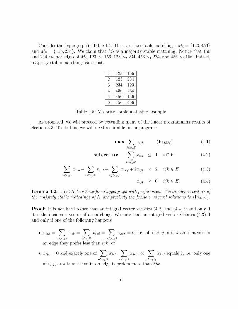
Consider the hypergraph in Table 4.5. There are two stable matchings: M5 = {123, 456}and M6 = {156, 234}. We claim that M5 is a majority stable matching: Notice that 156and 234 are not edges of M5, 123 >1 156, 123 >2 234, 456 >4 234, and 456 >5 156. Indeed,majority stable matchings can exist.

1 123 1562 123 2343 234 1234 456 2345 456 1566 156 456

Table 4.5: Majority stable matching example

As promised, we will proceed by extending many of the linear programming results ofSection 3.3. To do this, we will need a suitable linear program:

max∑

ijk∈E

xijk (PMSM) (4.1)

subject to:∑

uv:iuv∈E

xiuv ≤ 1 i ∈ V (4.2)

∑

ab>ijk

xiab +∑

cd>jik

xjcd +∑

ef>kij

xkef + 2xijk ≥ 2 ijk ∈ E (4.3)

xijk ≥ 0 ijk ∈ E. (4.4)

Lemma 4.2.1. Let H be a 3-uniform hypergraph with preferences. The incidence vectors ofthe majority stable matchings of H are precisely the feasible integral solutions to (PMSM).

Proof: It is not hard to see that an integral vector satisfies (4.2) and (4.4) if and only ifit is the incidence vector of a matching. We note that an integral vector violates (4.3) ifand only if one of the following happens:

• xijk =∑

ab>ijk

xiab =∑

cd>jik

xjcd =∑

ef>kij

xkef = 0, i.e. all of i, j, and k are matched in

an edge they prefer less than ijk, or

• xijk = 0 and exactly one of∑

ab>ijk

xiab,∑

cd>jik

xjcd, or∑

ef>kij

xkef equals 1, i.e. only one

of i, j, or k is matched in an edge it prefers more than ijk.

51

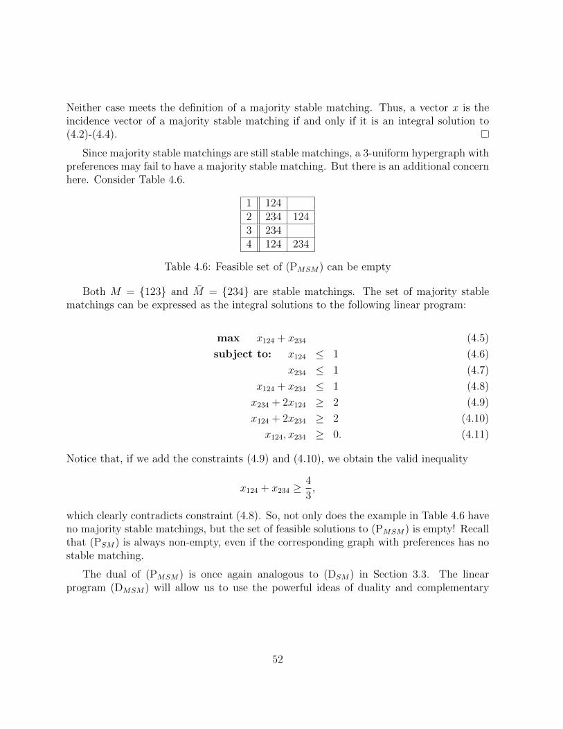
Neither case meets the definition of a majority stable matching. Thus, a vector x is theincidence vector of a majority stable matching if and only if it is an integral solution to(4.2)-(4.4).

Since majority stable matchings are still stable matchings, a 3-uniform hypergraph withpreferences may fail to have a majority stable matching. But there is an additional concernhere. Consider Table 4.6.

1 1242 234 1243 2344 124 234

Table 4.6: Feasible set of (PMSM) can be empty

Both M = {123} and M = {234} are stable matchings. The set of majority stablematchings can be expressed as the integral solutions to the following linear program:

max x124 + x234 (4.5)

subject to: x124 ≤ 1 (4.6)

x234 ≤ 1 (4.7)

x124 + x234 ≤ 1 (4.8)

x234 + 2x124 ≥ 2 (4.9)

x124 + 2x234 ≥ 2 (4.10)

x124, x234 ≥ 0. (4.11)

Notice that, if we add the constraints (4.9) and (4.10), we obtain the valid inequality

x124 + x234 ≥4

3,

which clearly contradicts constraint (4.8). So, not only does the example in Table 4.6 haveno majority stable matchings, but the set of feasible solutions to (PMSM) is empty! Recallthat (PSM) is always non-empty, even if the corresponding graph with preferences has nostable matching.

The dual of (PMSM) is once again analogous to (DSM) in Section 3.3. The linearprogram (DMSM) will allow us to use the powerful ideas of duality and complementary

52

slackness to obtain results that are analogous to the results in Section 3.3:

min∑

i∈V

yi − 2∑

ijk∈E

zijk (DMSM)

subject to: yi ≥ 0 i ∈ Vzijk ≥ 0 ijk ∈ E

yi + yj + yk −∑

jk>iab

ziab −∑

ik>jcd

zjcd −∑

ij>kef

zkef − 2zijk ≥ 1 ijk ∈ E.

Lemma 4.2.2. Let x be a feasible solution to (PMSM) and let y ∈ RV and z ∈ RE bedefined as follows:

yi =∑

uv:iuv∈E

xiuv i ∈ V,

zijk = xijk ijk ∈ E.

Then (y, z) is a feasible solution to (DMSM).

Proof: By construction, we see that yi ≥ 0 for all i ∈ V and zijk ≥ 0 for all ijk ∈ E.To establish the feasibility of (y, z), we consider the remaining constraint of (DMSM). Letijk ∈ E. For (y, z) the left hand side of the inequality is

yi + yj + yk −∑

jk>iab

ziab −∑

ik>jcd

zjcd −∑

ij>kef

zkef − 2zijk.

Substituting in the values for y and z we obtain

∑

ab:iab∈E

xiab +∑

cd:jcd∈E

xjcd +∑

ef :kef∈E

xkef −∑

jk>iab

xiab −∑

ik>jcd

xjcd −∑

ij>kef

xkef − 2xijk,

which simplifies to

∑

ab>ijk

xiab +∑

cd>jik

xjcd +∑

ef>kij

xkef + xijk ≥ 1.

The inequality in the last line follows from the primal feasibility of x. Thus, (y, z) is feasiblefor (DMSM).

In Section 3.3 we saw that every feasible solution to (PSM) was also an optimal solution.The linear program (PMSM) has the same helpful property.

53

Theorem 4.2.3. Let x be a feasible solution to (PMSM). Then x is also an optimal solutionto (PMSM).

Proof: Let x be a feasible solution to (PMSM). Define (y, z) as in Lemma 4.2.2. Since(y, z) is feasible for (DMSM), we can compute its objective value:

∑

i∈V

yi − 2∑

ijk∈E

zijk =∑

i∈V

∑

uv:iuv∈E

xiuv

− 2

∑

ijk∈E

xijk

= 3∑

ijk∈E

xijk − 2∑

ijk∈E

xijk

=∑

ijk∈E

xijk.

Since the dual objective value of (y, z) equals the primal objective value of x, Corollary1.1.3 implies that x is optimal for (PMSM).

We note that the proof of this result also shows that (y, z), defined in Lemma 4.2.2, isoptimal for (DMSM).

Theorem 4.2.4. Let H = (V,E, L) be a 3-uniform hypergraph with preferences. There isa partition (A,B) of V such that for every feasible solution, x, to (PMSM),

∑

uv:iuv∈E

xiuv = 1 if i ∈ A, and

∑

uv:iuv∈E

xiuv = 0 if i ∈ B.

Proof: Define the sets A and B as follows:

A =

v ∈ V :

∑

uv:iuv∈E

xiuv = 1 for all feasible x of (PMSM)

and

B =

v ∈ V :

∑

uv:iuv∈E

xiuv = 0 for all feasible x of (PMSM)

.

Let i ∈ V and suppose i 6∈ B. We will show i ∈ A. Since i 6∈ B, there exists a feasiblesolution x to (PMSM) such that ∑

uv:iuv∈E

xiuv > 0.

54

Define (y, z) as in Lemma 4.2.2. The proof of Theorem 4.2.3 shows that (y, z) is optimalfor (DMSM). Therefore, (x, (y, z)) satisfies the conditions of Theorem 1.1.4. Note that yiis the dual variable corresponding to the primal constraint

∑

uv:iuv∈E

xiuv ≤ 1.

Sinceyi =

∑

uv:iuv∈E

xiuv > 0,

Theorem 1.1.4 implies that ∑

uv:iuv∈E

xiuv = 1. (4.12)

Now, Theorem 4.2.3 tells us that every x which is feasible for (PMSM) is also optimal. So,(x, (y, z)) satisfies complementary slackness for all x feasible for (PMSM). In particular,(4.12) holds for all such x. Thus, i ∈ A.

This is exactly the same partition we saw for graphs with preferences in Sections 2.3and 3.3. Not surprisingly, this partition of the vertices leads to the same consequences.

Corollary 4.2.5. Let H be a 3-uniform hypergraph with preferences. For every feasiblesolution x to (PMSM),

∑

ijk∈E

xijk =|A|3.

Proof: Let x be a feasible solution to (PMSM). Recall from Theorem 4.2.4:

∑

uv:iuv∈E

xiuv = 1 if i ∈ A, and

∑

uv:iuv∈E

xiuv = 0 if i ∈ B.

55

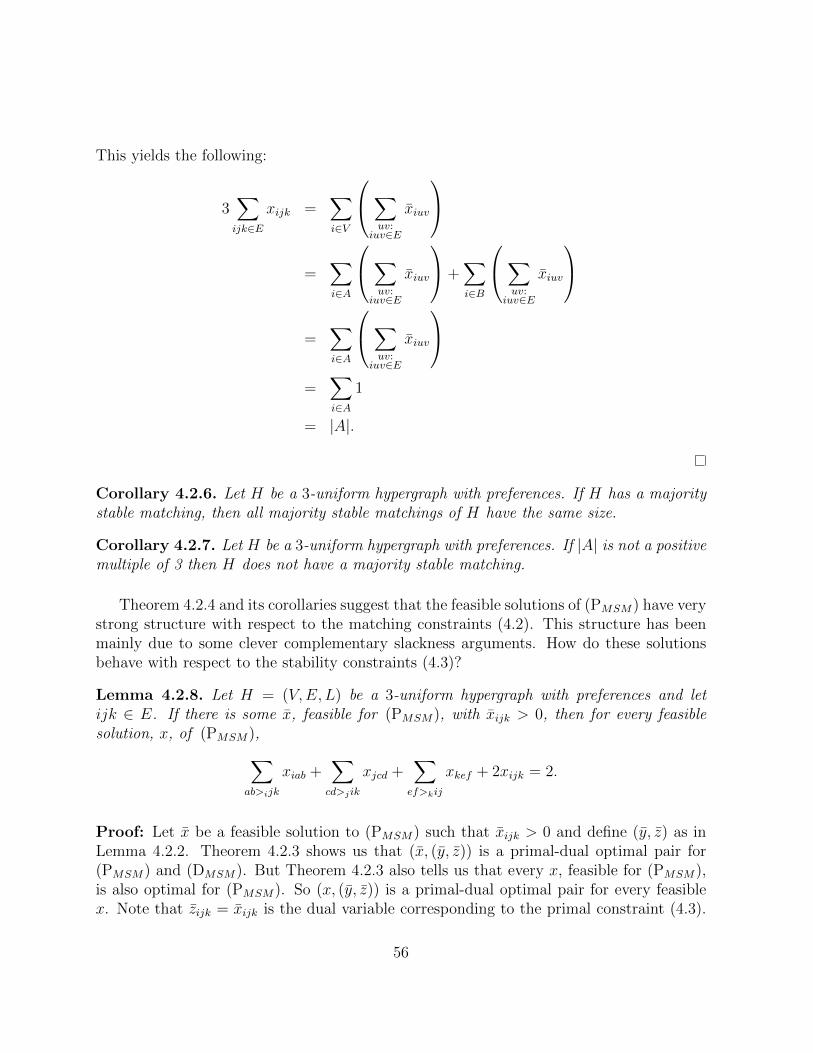
This yields the following:

3∑

ijk∈E

xijk =∑

i∈V

∑

uv:iuv∈E

xiuv

=∑

i∈A

∑

uv:iuv∈E

xiuv

+

∑

i∈B

∑

uv:iuv∈E

xiuv

=∑

i∈A

∑

uv:iuv∈E

xiuv

=∑

i∈A

1

= |A|.

Corollary 4.2.6. Let H be a 3-uniform hypergraph with preferences. If H has a majoritystable matching, then all majority stable matchings of H have the same size.

Corollary 4.2.7. Let H be a 3-uniform hypergraph with preferences. If |A| is not a positivemultiple of 3 then H does not have a majority stable matching.

Theorem 4.2.4 and its corollaries suggest that the feasible solutions of (PMSM) have verystrong structure with respect to the matching constraints (4.2). This structure has beenmainly due to some clever complementary slackness arguments. How do these solutionsbehave with respect to the stability constraints (4.3)?

Lemma 4.2.8. Let H = (V,E, L) be a 3-uniform hypergraph with preferences and letijk ∈ E. If there is some x, feasible for (PMSM), with xijk > 0, then for every feasiblesolution, x, of (PMSM),

∑

ab>ijk

xiab +∑

cd>jik

xjcd +∑

ef>kij

xkef + 2xijk = 2.

Proof: Let x be a feasible solution to (PMSM) such that xijk > 0 and define (y, z) as inLemma 4.2.2. Theorem 4.2.3 shows us that (x, (y, z)) is a primal-dual optimal pair for(PMSM) and (DMSM). But Theorem 4.2.3 also tells us that every x, feasible for (PMSM),is also optimal for (PMSM). So (x, (y, z)) is a primal-dual optimal pair for every feasiblex. Note that zijk = xijk is the dual variable corresponding to the primal constraint (4.3).

56

Since zijk > 0, complementary slackness tells us that (4.3) is satisfied with equality forevery feasible x.

Let M and M be stable matchings of a hypergraph with preferences. We will say thatvertex v prefers M to M if v prefers its matching edge in M to its matching edge in M .

Corollary 4.2.9. Let H be a 3-uniform hypergraph with preferences and let M be a ma-jority stable matching of H. If ijk ∈M , then there is no majority stable matching, M , ofH such that all of i, j, and k prefer M to M .

Proof: Let xM be the incidence vector of the majority stable matching M such thatijk ∈ M . Suppose, for a contradiction, that there exists a majority stable matching Msuch that all of i, j, and k prefer M to M and let xM be the incidence vector of M . Notethat xMijk = 0. Since xMijk = 1, Lemma 4.2.8 shows that

∑

ab>ijk

xMiab +∑

cd>jik

xMjcd +∑

ef>kij

xMkef = 2. (4.13)

However, all of i, j, and k prefer M to M . So

∑

ab>ijk

xMiab = 1,

∑

cd>jik

xMjcd = 1, and

∑

ef>kij

xMkef = 1.

This contradicts (4.13) and gives us the result.

Corollary 4.2.9 is of similar flavour to Corollary 2.1.6 from Section 2.1.1: Improvingthe outcome of a sufficiently large group of people will almost undoubtedly come at theexpense of another group of people.

Sadly, all this exciting work cannot hide the fact that majority stable matchings inhypergraphs with preferences can still pose difficulties. To illustrate this point, considerthe following disheartening result.

Theorem 4.2.10. If H is a 3-uniform hypergraph with preferences and H has a majoritystable matching, then H has only one majority stable matching.

Proof: LetH be a 3-uniform hypergraph with preferences and suppose, for a contradiction,that M and M are distinct majority stable matchings of H. Let T be the set of edgeswhich are in M but not in M and let U be the set of edges which are in M but not M .

57

Define W to be the set of vertices of H that are matched in M by the edges of T . Noticethat the vertex partition from Theorem 4.2.4 shows us that W is also the set of verticesmatched in M by the edges of U . Furthermore, |W | is a positive multiple of 3.

Now, xMijk = 1 > 0 for every ijk ∈ T . Therefore, by Lemma 4.2.8,

∑

ab>ijk

xiab +∑

cd>jik

xjcd +∑

ef>kij

xkef + 2xijk = 2

holds for the incidence vector, x, of any majority stable matching of H. Since xMijk = 0 forevery ijk ∈ T , ∑

ab>ijk

xMiab +∑

cd>jik

xMjcd +∑

ef>kij

xMkef = 2.

This tells us that for every ijk ∈ T , exactly two of i, j, and k prefer M to M . In simpleterms, two thirds of the vertices in W prefer M to M . However, if we repeat the argumentfor the edges of U , we will also see that two thirds of the vertices in W prefer M to M .The result follows from this contradiction.

Theorem 4.2.10 rules out any further discussion of the set of majority stable matchingsfor a particular 3-uniform hypergraph. However, if we were given the task of finding astable matching in a 3-uniform hypergraph with preferences, a majority stable matchingwould be a desirable choice because of the increased agreement among the vertices. Isthere a large class of 3-uniform hypergraphs with preferences that will have a majoritystable matching? In point of fact, the class is much larger than the class of graphs withpreferences that have a stable matching.

4.2.1 Constructing Majority Stable Matchings

In some sense, majority stable matchings are the ideal stable matchings in 3-uniformhypergraphs with preferences. The problem is that they do not always exist. We wouldlike to construct an infinite class of 3-uniform hypergraphs with preferences that have amajority stable matching.

Our construction starts with a graph with preferences, G, and a fixed stable matchingof G, say M . We will build a 3-uniform hypergraph with preferences, H(G; M) = (V,E, L),using the structure of G and M . Specifically, let G = (V , E, L) be a graph with preferencesthat has at least one stable matching and let M be a stable matching of G. The verticesof H(G; M) are given by

V := V ∪ {zxy : xy ∈ M}.That is, the vertices of H(G; M) are the vertices of G plus a vertex for each edge of M . Todefine the edges of H(G; M), we first choose a subset of edges, Tzxy , of G for every xy ∈ M .

58

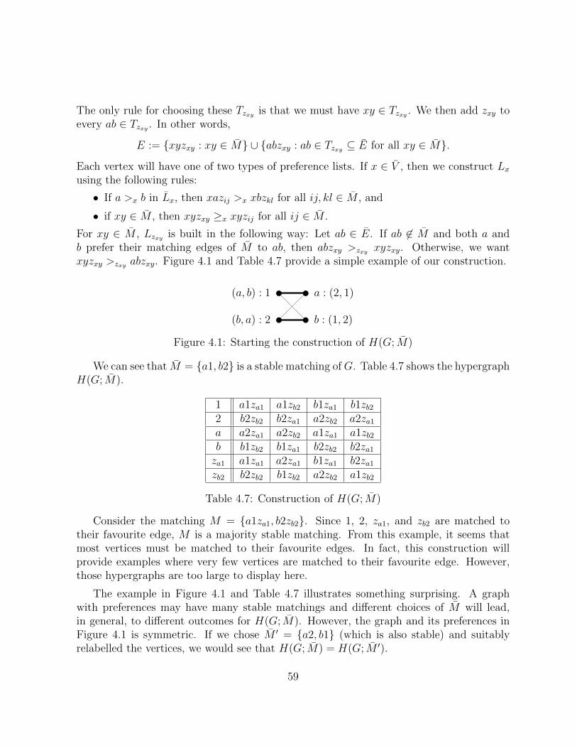
The only rule for choosing these Tzxy is that we must have xy ∈ Tzxy . We then add zxy toevery ab ∈ Tzxy . In other words,

E := {xyzxy : xy ∈ M} ∪ {abzxy : ab ∈ Tzxy ⊆ E for all xy ∈ M}.Each vertex will have one of two types of preference lists. If x ∈ V , then we construct Lx

using the following rules:

• If a >x b in Lx, then xazij >x xbzkl for all ij, kl ∈ M , and

• if xy ∈ M , then xyzxy ≥x xyzij for all ij ∈ M .

For xy ∈ M , Lzxy is built in the following way: Let ab ∈ E. If ab 6∈ M and both a andb prefer their matching edges of M to ab, then abzxy >zxy xyzxy. Otherwise, we wantxyzxy >zxy abzxy. Figure 4.1 and Table 4.7 provide a simple example of our construction.

(a, b) : 1

(b, a) : 2

a : (2, 1)

b : (1, 2)

Figure 4.1: Starting the construction of H(G; M)

We can see that M = {a1, b2} is a stable matching ofG. Table 4.7 shows the hypergraphH(G; M).

1 a1za1 a1zb2 b1za1 b1zb22 b2zb2 b2za1 a2zb2 a2za1

a a2za1 a2zb2 a1za1 a1zb2b b1zb2 b1za1 b2zb2 b2za1

za1 a1za1 a2za1 b1za1 b2za1

zb2 b2zb2 b1zb2 a2zb2 a1zb2

Table 4.7: Construction of H(G; M)

Consider the matching M = {a1za1, b2zb2}. Since 1, 2, za1, and zb2 are matched totheir favourite edge, M is a majority stable matching. From this example, it seems thatmost vertices must be matched to their favourite edges. In fact, this construction willprovide examples where very few vertices are matched to their favourite edge. However,those hypergraphs are too large to display here.

The example in Figure 4.1 and Table 4.7 illustrates something surprising. A graphwith preferences may have many stable matchings and different choices of M will lead,in general, to different outcomes for H(G; M). However, the graph and its preferences inFigure 4.1 is symmetric. If we chose M ′ = {a2, b1} (which is also stable) and suitablyrelabelled the vertices, we would see that H(G; M) = H(G; M ′).

59

Lemma 4.2.11. Let G be a graph with preferences and let M be a stable matching of G.Then H(G; M) has a majority stable matching.

Proof: Let G be a graph with preferences and let M be a stable matching of G. DefineM := {xyzxy : xy ∈ M}. We will show that M is a majority stable matching of H(G; M).By construction, M is certainly a matching of H(G; M). Suppose, for a contradiction, thatM is not a majority stable matching. Then, there exists an edge ijzxy, for some xy ∈ M ,such that at least two of i, j, and zxy prefer ijzxy to their respective matching edges.

Notice that if ijzxy >zxy xyzxy, then, by the construction of Lzxy , ij 6∈ M and bothi and j prefer their matching edges of M to ij. So, i and j also prefer their matchingedges of M to ijzxy. Hence, zxy is the only vertex of i, j, and zxy that prefers ijzxy toits matching edge. This would contradict that ijzxy is a blocking edge of M . So, we mayassume that only i and j prefer ijzxy.

Suppose ikzik ∈ M , so that ik ∈ M . By construction of Li, ikzik is i’s most preferrededge that contains k. So, if i prefers ijzxy to ikzik, then j 6= k and j >i k in Li. Similarly, jprefers i to its matching partner of M . Therefore, ij is a blocking edge of M , contradictingthat M is a stable matching of G. Thus, M is indeed a majority stable matching ofH(G; M).

The construction of H(G; M) takes a graph with preferences and a stable matching tocreate a 3-uniform hypergraph with preferences and a majority stable matching. Couldthere be a converse to this statement? In other words, does every 3-uniform hypergraphwith a majority stable matching correspond in some natural way to a graph with a stablematching? Currently, we do not know the answer to this question, but we can show aresult of this form for a certain special class of hypergraphs.

So far, the graphs we considered have been simple: For each pair of vertices, x and y,there is, at most, one edge of the form xy. For the remainder of this section, we are goingto relax this requirement and allow pairs of vertices to have multiple edges between them.For a fixed pair of vertices, x and y, the set of edges that have both x and y as endpointsis called the parallel class of x and y. The graphs which allow parallel classes bigger thanone are called multigraphs.

Conveniently, the definition of “stable matching” is the same for graphs and multi-graphs. In 2005, Cechlarova and Fleiner showed that finding a stable matching in a multi-graph with preferences is equivalent to finding a stable matching in graph with preferences.Specifically, they showed that if H is a multigraph with preferences, then there is a sim-ple graph with preferences, G, such that H has a stable matching if and only if G has astable matching. Consequently, Irving’s algorithm can be used to find a stable matchingin a multigraph with preferences by finding a stable matching in a suitable graph withpreferences. We will refer the reader to the paper of Cechlarova and Fleiner for moredetails [9].

60

Let H = (V,E, L) be a 3-uniform hypergraph with preferences. We will call H bipartiteif there exists a set X ⊆ V such that every edge of H contains exactly one vertex ofX. Notice that, in a bipartite 3-uniform hypergraph, the neighbourhood of X, N(X),induces a multigraph. This multigraph, H[N(X)], has vertex set N(X) and edge set{(yz)x : x ∈ X and xyz ∈ E}.

There is a natural way to define the preference lists of N(X) based on L. Observe thatthere is a one-to-one correspondence between the edges of H and the edges of H[N(X)].Therefore, if xyz >y xyz in H, we will insist that (yz)x >y (yz)x in H[N(X)] for allx ∈ X and y, z, z ∈ N(X). With this requirement, we will say that H[N(X)] has inducedpreferences. Table 4.8 illustrates the close relationship between the preference lists of Hand the preference lists of H[N(X)].

H y xyz xyz xyz xyzH[N(X)] y (yz)x (yz)x (yz)x (yz)x

Table 4.8: Preference lists of N(X) in H and H[N(X)]

Lemma 4.2.12. Let H = (V,E, L) be a bipartite 3-uniform hypergraph with preferencesand let X ⊆ V be its distinguished set of vertices. If H has a majority stable matching,then H[N(X)] with induced preferences has a stable matching.

Proof: Suppose H = (V,E, L) is a 3-uniform hypergraph with preferences and let X bea set of vertices such that every e ∈ E contains exactly one vertex of X. Let M be amajority stable matching of H. Define M := {(yz)x : xyz ∈ M and x ∈ X}. We will showthat M is a stable matching of H[N(X)]. The set M is certainly a matching of H[N(X)].Suppose, for a contradiction, that M is not a stable matching of H[N(X)]. Then thereexists an edge of H[N(X)], say (ab)x, that blocks M .

Since (ab)x 6∈ M , the construction of M tells us that xab 6∈ M . Since M is a majoritystable matching, at least two of x, a, and b prefer their respective matching edges of M toxab. However, the correspondence between the preference lists of H and H[N(X)] showsthat at least one of a or b prefers its matching edge of M to (ab)x, contradicting that (ab)xwas a blocking edge of M . Thus, M is a stable matching of H[N(X)].

Suppose that M is a stable matching of H[N(X)]. We can define a simple graph withpreferences, G, by deleting all but one edge from each parallel class, while preserving theedges of M . The preference lists of G are obtained from H[N(X)] by simply deleting theentries corresponding to the edges that were deleted. Then if M is a stable matching ofH[N(X)], M remains stable in G because we did not delete any edges of M . As with ourconstruction of H(G; M), this G is not unique. Different choices of edge deletions will giveus, in general, different graphs with preferences.

61

Another question which we did not answer here is: Can we decide if a 3-uniformhypergraph with preferences has a majority stable matching? At the moment, it is unclearif the feasibility of (PMSM) is sufficient to guarantee a majority stable matching or if(PMSM) can be feasible without an integral solution. In the next chapter, we will discusssome other open problems relating to 3-uniform hypergraphs.

62

Chapter 5

Concluding Remarks

The practical applications of stable matchings have been evident since their formal intro-duction in 1962. Indeed, the Gale-Shapley algorithm has been used to solve instances ofthe college admissions problem for the NRMP and, in some cases, real schools. Today,the medical field has found more complicated applications of hypergraphic stable match-ings [24]. Stable matchings have even been applied in many other areas of mathematics [33].A surprising fact to many people is that rich structure can be found when stable match-ings are considered as a theoretical object. This versatility has helped the theory of stablematchings to become a popular and developed research topic.

Before we continue on to some interesting unsolved problems, let us summarize whatwe have seen in the preceding chapters.

Chapter 2We began with an introduction to graphs with preferences and the basics of stable match-ings. We then saw that the proposal/rejection process used by Gale and Shapley led tosome very intriguing properties. We also looked into stable matchings in non-bipartitegraphs with preferences. Irving’s algorithm showed that many of the interesting stablematching properties found in bipartite graphs remain in stable matchings of non-bipartitegraphs.

As an aside, we looked briefly at the intimate connection between stable matchings andlattice theory. Delving further into this association would require much more time thanwe have here, but is a fascinating subject in its own right.

Chapter 3Chapter 3 focused on the following question: “Can we generalize Theorem 2.1.1 to non-bipartite graphs with preferences?” In fact, this is achieved by relaxing the integrality ofa stable matching to allow edges to take fractional values. But, rather than attacking

63

non-bipartite graphs directly, we looked to fractional stable matchings in hypergraphswith preferences. Using a matrix version of a powerful result due to Scarf, Theorem 3.1.2promised that EVERY hypergraph with preferences has a fractional stable matching. Wethen applied Theorem 3.1.2 to the special case of graphs. We saw that every graph withpreferences contains a set of edges that is, at least, very similar to a stable matching. As aconsequence of this fact, we can characterize the graphs with preferences that admit stablematchings.

Linear programming provided tools that enabled us to talk about stable matchingsand fractional stable matchings at the same time. This allowed us to prove that fractionalstable matchings have analogous properties to stable matchings in graphs with preferences.

Chapter 4Contrary to stable matchings in graphs with preferences, stable matchings in hypergraphswith preferences behave very badly. The remarkable properties evident in graphs withpreferences vanish when edges are allowed to have a size bigger than two. The lack ofthese properties is likely the reason why most hypergraphic stable matching problems areNP-complete.

By considering majority stable matchings, we were able to use linear programming toour advantage again. However, our successes were fleeting. The existence of a majoritystable matching in a 3-uniform hypergraph with preferences is such a strong propertythat there can be, at most, one. However, we saw that it is possible to construct a largeclass of 3-uniform hypergraphs with preferences which admit majority stable matchings.This construction uncovered a strong relationship between majority stable matchings in3-uniform hypergraphs and stable matchings in graphs.

5.1 Open Questions

To conclude this thesis, we will look to the future and discuss two open problems aboutstable matchings in 3-uniform hypergraphs with preferences.

5.1.1 The Cyclic Stable Family Problem

Our first open problem is a slight variation on the stable family problem. It is rumoured tobe due to Knuth, but it first appeared in a paper by Ng and Hirschberg after they provedthat the stable family problem was NP-complete [37]. Specifically, we are interested in thefollowing:

Problem 6 (Cyclic Stable Family Problem). A community consists of n men, n women,and n dogs. Each man ranks every woman in terms of with whom they would prefer to be

64

in a family. Similarly, each woman ranks all the dogs and each dog ranks all the men. Canwe find a set of families such that if a man, a woman, and a dog are not a family then atleast one of them prefers their current family?

Once again, we are looking for a stable matching in a tripartite 3-uniform hypergraphwith preferences, H = (A ∪ B ∪ C,E, L). The difference here comes in the structure ofthe preference lists. Notice that each vertex no longer ranks all its adjacent neighbours:The vertices of A are interested only in the vertices of B, B is interested only in C, and Cis interested only in A. For example, if i ∈ A and j ∈ B, then any edge containing bothi and j is the same from i’s perspective. In this situation, we will say that H has cyclicpreferences.

With this special type of preference list, the definition of a blocking edge remains thesame: A blocking edge for a matching M of H is an edge ijk 6∈ M such that all of i, j,and k prefer ijk to their respective matching edges. A matching, M , is stable if it doesnot have any blocking edges.

For the remainder of this section, we will make two assumptions:

• For every i ∈ A, j ∈ B, and k ∈ C, ijk is an edge of H, and

• n = |A| = |B| = |C|.The first assumption simply says that H is a complete hypergraph. This problem becomesNP-complete without the completeness restriction [6]. The second assumption is purelyaesthetic. If the vertex classes have different sizes, then we can add just enough artificialvertices so that A, B, and C are the same size. Any of these artificial vertices will beappended to the end of any preference lists in an arbitrary order. Then, if the new hyper-graph has a stable matching M , we can exclude any edge of M that contains any of theartificial vertices to obtain a stable matching of the original hypergraph.

To some extent, this variant of the stable family problem most closely resembles theoriginal stable marriage problem: Each vertex class has preferences over only one other ver-tex class. Recall that every instance of the stable marriage problem has a stable matching.The belief is that this fact is also true for the cyclic stable family problem.

Conjecture 5.1.1 (Eriksson, Sjostrand, and Strimling [10]). Every tripartite 3-uniformhypergraph with cyclic preferences has a stable matching.

How close are we to a proof of this conjecture? Actually, not close at all. At this pointin time, we know only that very small instances always admit stable matchings.

Theorem 5.1.2 (Eriksson, Sjostrand, and Strimling [10]). Let H be a tripartite 3-uniformhypergraph with cyclic preferences. If n ≤ 4, then H has a stable matching.

65

The proof of this result is a highly technical case analysis that is difficult to extend tolarger values of n. Additionally, Eriksson, Sjostrand, and Strimling provided substantialcomputer evidence to suggest that the n = 5 case is true [10]. However, a formal proof ofthis fact remains elusive. We would suspect that successful proofs of the full conjecturewould cleverly employ one of two strategies:

• Generalize the Gale-Shapley algorithm to account for the extra vertex class, or

• artificially define a second set of preferences for the vertices of A over the vertices ofC and then use a double application of Theorem 2.1.1.

Since we are unable to resolve Conjecture 5.1.1, nor the n = 5 case, in this thesis (perhapsat a later date), we will look at some special cases.

Lemma 5.1.3. Let H = (A ∪ B ∪ C,E, L) be a 3-uniform, tripartite hypergraph withcyclic preferences. If every vertex in A has the same preference list, then H has a stablematching.

Proof: We proceed by induction on n. If n ≤ 4, then H has a stable matching by Theorem5.1.2. So, we can assume that n ≥ 5 and that the result holds for all k < n. Supposefurther that y ∈ B is the most preferred vertex by the vertices of A, z ∈ C is the favouritevertex of y, and x ∈ A is the favourite vertex of z.

Consider the subhypergraph with preferences, T , obtained by removing the vertices x,y, and z from H. By the inductive hypothesis, T has a stable matching M . Define thematching M := M ∪ {xyz} for H.

Claim: The matching M is a stable matching of H.

Proof of Claim: Suppose, for a contradiction, that M is not a stable matching. Then thereexists a blocking edge ijk for M . Notice that any ijk must contain one of the vertices x,y, or z. Otherwise, ijk would also be a blocking edge for M in T , contradicting that M isa stable matching of T . Now, recall that xyz ∈M . Therefore, the vertices x, y, and z arealready matched to their most preferred vertex. Thus, the blocking edge ijk cannot exist.This contradiction shows that M is a stable matching of T .

Notice that we could strengthen this result slightly: Instead of restricting the verticesof A to a single preference list, we could just insist that the first n− 4 entries are identical.

Lemma 5.1.4. Let H = (A∪B ∪C,E, L) be a tripartite 3-uniform hypergraph with cyclicpreferences. If each vertex of A has a distinct favourite vertex in B, then H has a stablematching.

Proof: Let M be any matching of H such that each vertex in A is matched in an edgecontaining its favourite vertex of B.

66

Claim: The matching M is a stable matching of H.

Proof of Claim: Suppose, for a contradiction, that M is not stable. Then, there exists ablocking edge ijk for M . We may assume that i ∈ A. By definition of M , i is alreadymatched to its favourite vertex, meaning that the vertex j cannot exist. This contradictsthat ijk is a blocking edge for M . Thus, M is a stable matching.

An edge ijk is a preferable edge if j is first in i’s preference list, k is first in j’s preferencelist, and i is first in k’s preference list. In the n = 5 case, the existence of a preferable edgeis sufficient to guarantee the existence of a stable matching and follows from Lemma 5.1.3.

Lemma 5.1.5. Let H = (A∪B ∪C,E, L) be a tripartite 3-uniform hypergraph with cyclicpreferences where n = 5. If H has a preferable edge, then H has a stable matching.

As anyone who has been part of a committee will know, the unanimous agreement ofLemma 5.1.3 is an exceedingly special case. Even the complete discord of Lemma 5.1.4and the ideal triple of Lemma 5.1.5 are very rare. But, these extreme cases make stablematching proofs quite pleasant. To have any hope of proving Conjecture 5.1.1, we willneed to fill in this gap. Sadly, this is quite a substantial challenge when we do not knowof a way to extend the work of Gale and Shapley. To partially illustrate this fact, let usconsider the n = 5 case.

Lemma 5.1.6. Let H = (A∪B ∪C,E, L) be a tripartite 3-uniform hypergraph with cyclicpreferences where n = 5. If there are two vertices of B that are first and second in everypreference list of A, then H has a stable matching.

Proof: Let H = (A ∪ B ∪ C,E, L) be a tripartite 3-uniform hypergraph with cyclicpreferences where n = 5. Suppose b, b ∈ B are the two vertices described in the statementof the lemma. Let Ab be the subset of vertices of A that rank b first and b second. Similarly,let Ab be the vertices of A that rank b first and b second. Notice that, by assumption,(Ab, Ab) is a partition of A.

Let c and c in C be the favourite vertices of b and b, and let a and a in A be thefavourite vertices of c and c, respectively.

At this point, we can make the following assumptions:

• c 6= c,

• a 6= a, and

• a ∈ Ab and a ∈ Ab.

If c = c, then either abc or abc is a preferable edge, depending on whether a ∈ Ab ora ∈ Ab. Therefore by Lemma 5.1.5, H has a stable matching. Similarly, we can findpreferable edges if a = a, a ∈ Ab, or a ∈ Ab.

67

Now, consider the subhypergraph, T , of H obtained by removing the vertices a, a, b, b,c, and c. By Theorem 5.1.2, T has a stable matching, say M . Define M := M ∪{abc, abc},a matching of H.

Claim: The matching M is a stable matching of H.

Proof of Claim: Suppose, for a contradiction, that M is not stable. Then, there existsa blocking edge ijk for M . Since M is a stable matching for T and b, b, c, and c arematched in M to their favourite vertices, we can say that the edge ijk contains either aor a. Suppose i = a. Since a ∈ Ab and abc ∈ M , the only vertex a prefers to b is b. Butb is matched to c, its favourite vertex of C. Therefore it is not possible for ijk to be ablocking edge, contradicting that M was not a stable matching. This contradiction givesus the result.

This proof relies on the three assumptions that guarantee a preferable edge. But veryfew instances of the cyclic stable family problem actually have a preferable edge. Thismeans that we have to consider edges that are not as well liked by their vertices, drivingthe number of cases out of control very quickly. We hope that a more cunning approach ispossible.

5.1.2 Bounded Denominators

In Chapter 3, we saw that every graph with preferences has a stable partition. As aconsequence of this, every graph with preferences also has a half-integral stable matching.It is natural to wonder if 3-uniform hypergraphs have a similar fractional stable matching.With a bit of work, or a quick trip back to Table 4.4 in Section 4.1, we see that it is notpossible for all hypergraphs with preferences to have a half-integral stable matching. So,what kinds of edge values can we hope for? Are they even rational? More concretely, can wefind some absolute constant N such that for every 3-uniform hypergraph with preferences,there is a fractional stable matching where the denominator of every fractional value is atmost N?

As an example, we saw that N = 2 for graphs. If such an N existed for 3-uniformhypergraphs, Table 4.4 shows that N = 3 is the best possible. We are interested in knowingif three is the true value of N for all 3-uniform hypergraphs. Before we continue, we willmake this notion precise. A fractional stable matching, x, is a 1

3-integral stable matching if

xe ∈ {0, 13, 1

2, 2

3, 1} for every e ∈ E. Based on this definition, we ask the following question:

Question 5.1.7. Does every 3-uniform hypergraph with preferences have a 13-integral stable

matching?

To clarify, a 3-uniform hypergraph may have many fractional stable matchings; someof which may even have arbitrarily large denominators. We would like to know if at least

68

one of the fractional stable matchings has reasonable values. At this point, we do not knowthe answer to this problem. However, there is some evidence to suggest it might be true.

Lemma 5.1.8. Let H = (V,E, L) be a hypergraph with preferences and let x be a fractionalstable matching of H. The support of x, supp(x), has at most |V | edges.

Proof: Let H = (V,E, L) be a 3-uniform hypergraph with preferences. Let x be afractional stable matching ofH and let S = supp(x). Since x is a fractional stable matching,we can orient each edge e towards a vertex v such that

∑e≤vj

xj = 1. The following claimshows that |S| ≤ |V |, as required.

Claim: Each vertex v is the head of at most one arc in S.

Proof of Claim: Suppose vertex v is the head of arcs e, h ∈ S. Without loss of generality,we may assume that e <v h. Since v is the head of both e and h,

∑e≤vj

xj = 1 and∑h≤vj

xj = 1. But since e <v h, we must have xe = 0, contradicting that e ∈ S.

Lemma 5.1.8 tells us that the subhypergraph induced by the support of a fractionalstable matching is very sparse. This greatly reduces the number of eccentric special casesfor the structure of the support of a fractional stable matching.

Recall from Chapter 3 that we could show another result that is similar to the claimin the above proof: Each vertex v is the tail of at most one arc in S. With this secondproperty, it is possible to deduce the structure of S, and hence, define a half-integralstable matching. Ideally, we would like to be able to do something similar here. As wemight expect, however, this is the step that is currently missing. But, for small 3-uniformhypergraphs, it is feasible to attack the problem directly.

Lemma 5.1.9. Every 3-uniform hypergraph with preferences with four vertices has a 13-

integral stable matching.

Proof: Let H = (V,E, L) be a 3-uniform hypergraph with preferences where |V | = 4. Letx be a fractional stable matching of H and let S = supp(x). If |S| = 1, then S is a stablematching. So, we may assume that |S| ≥ 2.

Claim: The set S cannot contain exactly three edges.

Proof of Claim: Suppose, for a contradiction, that |S| = 3. Let a, b, c ∈ S. Since H hasonly four vertices, there must be exactly one vertex, v, that is incident to all of a, b, andc. Since x is a fractional stable matching, we must have

xa + xb + xc = 1. (5.1)

69

We may assume that a >v b >v c. The edge b must contain a vertex u 6= v such that∑

b≤uj

xj = 1,

as x is a fractional stable matching. Note that deg(u) = 2 in S, by the above remarks.However, this contradicts (5.1) since v is the only vertex incident to all of a, b, and c.Thus, it is not possible for |S| = 3.

Suppose |S| = 2 and let a, b ∈ S. Since H has only four vertices, the edges a and bmust share exactly two vertices, say u and v. Further, xa < 1 and xb < 1. Let z be thethird vertex of the edge a. Notice that if both a >u b and a >v b hold, then we must have

∑

a≤zj

xj = 1,

since x is a fractional stable matching. But, z is only incident to a in S. Therefore,∑

a≤zj

xj = xa < 1,

contradicting that x was a fractional stable matching. So, we must have a >u b and b >v a.Now, we can define a new fractional stable matching, x, by

xe =

{12

if e ∈ S0 otherwise.

The stability of x follows since supp(x) = supp(x).

If |S| = 4, then by the claim in the proof of Lemma 5.1.8, every edge of S must be lastin the preference list of some vertex. Simply set xe = 1

3for every e ∈ E to construct a

fractional stable matching.

In all cases, H has a 13-integral stable matching.

It is possible to extend this result to 3-uniform hypergraphs with |V | ≤ 5. However,it would be rather cruel to force the reader to suffer through the case-by-case verificationwhen the end of this thesis is so close. Hopefully, we will think of a clever way to simplifythe proof enough in the near future to make it presentable.

There is some disagreement about the potential answer to Question 5.1.7. In generalhypergraphs with preferences, it is known that the denominators in fractional stable match-ings can be unbounded. For example, consider the r-uniform analogue of Table 4.4. It ispossible to show that the best fractional stable matching assigns 1

rto each of the edges.

Once again, we will let the reader play with this problem (Hint: Notice the cyclic natureof the preferences). Perhaps, for 3-uniform hypergraphs, it is more realistic to hope thatthe denominators are simply bounded by a finite positive integer. In either case, we wouldlike to resolve this question.

70

Bibliography

[1] Hernan Abeledo and Garth Isaak. A characterization of graphs that ensure the exis-tence of stable matchings. Mathematical Social Sciences, 22(1):93 – 96, 1991. 21

[2] Hernan G. Abeledo and Yosef Blum. Stable matchings and linear programming. LinearAlgebra and its Applications, 245:321–333, 1996.

[3] Hernan G. Abeledo and Uriel G. Rothblum. Stable matchings and linear inequalities.Discrete Appl. Math., 54(1):1–27, 1994. 43, 44, 45

[4] Ron Aharoni and Tamas Fleiner. On a lemma of Scarf. J. Comb. Theory Ser. B,87(1):72–80, 2003. 32, 33, 36

[5] Dimitris Bertsimas and John Tsitsiklis. Introduction to Linear Optimization. AthenaScientific, 1997. 9

[6] Peter Biro and Eric McDermid. Three-sided stable matchings with cyclic preferences.Algorithmica, 58(1):5–18, 2009. 50, 65

[7] Charles Blair. Every finite distributive lattice is a set of stable matchings. J. Comb.Theory, Ser. A, 37(3):353–356, 1984. 20

[8] J.A. Bondy and U.S.R. Murty. Graph Theory, volume 244 of Graduate Texts inMathematics. Springer, 2008. 7

[9] Katarına Cechlarova and Tamas Fleiner. On a generalization of the stable roommatesproblem. ACM Trans. Algorithms, 1(1):143–156, 2005. 60

[10] Kimmo Eriksson, Jonas Sjostrand, and Pontus Strimling. Three-dimensional stablematching with cyclic preferences. Mathematical Social Sciences, 52(1):77 – 87, 2006.65, 66

[11] Tomas Feder. A new fixed point approach for stable networks and stable marriages.In STOC ’89: Proceedings of the twenty-first annual ACM symposium on Theory ofcomputing, pages 513–522, New York, NY, USA, 1989. ACM. 44

71

[12] Tamas Fleiner. Stable and Crossing Structures. PhD thesis, Technische UniversiteitEindhoven, 2000.

[13] D. Gale and L. S. Shapley. College admissions and the stability of marriage. TheAmerican Mathematical Monthly, 69(1):9–15, 1962. 3, 14, 15, 17

[14] David Gale and Marilda Sotomayor. Some remarks on the stable matching problem.Discrete Applied Mathematics, 11(3):223 – 232, 1985. 16

[15] Giorgio Gallo, Giustino Longo, Stefano Pallottino, and Sang Nguyen. Directed hy-pergraphs and applications. Discrete Appl. Math., 42(2-3):177–201, 1993.

[16] Fred Galvin. The list chromatic index of a bipartite multigraph. Journal of Combi-natorial Theory, Series B, 63(1):153 – 158, 1995. 3

[17] George Gratzer. Lattice Theory: First Concepts and Distributive lattices. W.H. Free-man and Company, San Francisco, California, 1971. 11

[18] Dan Gusfield, Robert Irving, Paul Leather, and Michael Saks. Every finite distributivelattice is a set of stable matchings for a small stable marriage instance. Journal ofCombinatorial Theory, Series A, 44(2):304 – 309, 1987. 20

[19] Dan Gusfield and Robert W. Irving. The stable marriage problem: structure andalgorithms. MIT Press, Cambridge, MA, USA, 1989. 16, 18, 20, 26, 27

[20] Penny Haxell. Stable matchings, October 2008. Lecture Notes, CO 342, University ofWaterloo.

[21] Penny Haxell. On forming committees. unpublished manuscript, University of Wa-terloo, 2010. 32, 33

[22] Penny Haxell and G. T. Wilfong. A fractional model of the border gateway protocol(BGP). In SODA ’08: Proceedings of the nineteenth annual ACM-SIAM symposiumon Discrete algorithms, pages 193 – 199, Philadelphia, PA, USA, 2008. Society forIndustrial and Applied Mathematics.

[23] Chien-Chung Huang. Two’s company, three’s a crowd: Stable family and threesomeroommates problems. In ESA, pages 558–569, 2007. 50

[24] Chien-Chung Huang. Circular stable matching and 3-way kidney transplant. Algo-rithmica, 58(1):137–150, 2009. 3, 50, 63

[25] J.S. Hwang. The algebra of stable marriages. Intern. J. Computer Math., 20(3-4):227–243, 1986. 20

72

[26] Robert W. Irving. An efficient algorithm for the ”stable roommates” problem. J.Algorithms, 6(4):577–595, 1985. 21, 23, 24, 25, 27, 28

[27] Robert W. Irving. Stable marriage and indifference. Discrete Appl. Math., 48(3):261–272, 1994. 50

[28] Robert W Irving and Paul Leather. The complexity of counting stable marriages.SIAM J. Comput., 15(3):655–667, 1986. 18, 20

[29] Robert W. Irving, Paul Leather, and Dan Gusfield. An efficient algorithm for the“optimal” stable marriage. J. ACM, 34(3):532–543, 1987.

[30] Robert W. Irving and David F. Manlove. The stable roommates problem with ties.Journal of Algorithms, 43(1):85 – 105, 2002.

[31] Kazuo Iwama, David Manlove, Shuichi Miyazaki, and Yasufumi Morita. Stable mar-riage with incomplete lists and ties. In ICALP, pages 443–452, 1999.

[32] Richard Karp. Reducibility among combinatorial problems. In Complexity of Com-puter Computations, pages 85 – 103. Plenum Press, 1972. 9, 44

[33] Donald E. Knuth. Mariages stables et leurs relations avec d’autres problemes combi-natoires. Les Presses de l’Universite de Montreal, Montreal, Quebec, 1976. 3, 16, 18,19, 20, 21, 63

[34] David F. Manlove, Robert W. Irving, Kazuo Iwama, Shuichi Miyazaki, and YasufumiMorita. Hard variants of stable marriage. Theor. Comput. Sci., 276(1-2):261–279,2002. 30

[35] D. G. McVitie and L. B. Wilson. Stable marriage assignment for unequal sets. BIT,10(3):295–309, 1970. 16

[36] D. G. McVitie and L. B. Wilson. The stable marriage problem. Commun. ACM,14(7):486–490, 1971. 17

[37] Cheng Ng and Daniel S. Hirschberg. Three-dimensional stable matching problems.SIAM Journal on Discrete Mathematics, 4:4–245, 1991. 48, 64

[38] National Resident Matching Program. http://www.nrmp.org/, 2010. 16

[39] Caroline Rioux. Scarf’s theorem and applications in combinatorics. Master’s thesis,University of Waterloo, 2006. 32, 33

[40] Eytan Ronn. NP-complete stable matching problems. Journal of Algorithms, 11(2):285– 304, 1990. 30

73

[41] Alvin E. Roth. The evolution of the labor market for medical interns and residents:A case study in game theory. Journal of Political Economy, 92:991 – 1016, 1984. 16

[42] Alvin E. Roth, Uriel G. Rothblum, and John H. Vande Vate. Stable matchings,optimal assignments, and linear programming. Math. Oper. Res., 18(4):803–828, 1993.43, 44, 45

[43] Alvin E. Roth, Tayfun Sonmez, and M. Utku Unver. Pairwise kidney exchange.Journal of Economic Theory, 125(2):151 – 188, 2005. 3

[44] Alvin E. Roth and Marilda Sotomayor. Two-sided matching: A study in game-theoreticmodeling and analysis. Cambridge University Press, 1990.

[45] Uriel G. Rothblum. Characterization of stable matchings as extreme points of apolytope. Math. Program., 54(1):57–67, 1992. 44

[46] Herbert E. Scarf. The core of an n person game. Cowles Foundation Discussion Papers182R, Cowles Foundation, Yale University, 1965. 32, 33

[47] Jimmy J. M. Tan. A maximum stable matching for the roommates problem. BIT,30(4):631–640, 1990. 39, 41

[48] Jimmy J. M. Tan. A necessary and sufficient condition for the existence of a completestable matching. J. Algorithms, 12(1):154–178, 1991. 34, 35, 36, 37, 39, 40, 41

[49] Chung-Piaw Teo and Jay Sethuraman. The geometry of fractional stable matchingsand its applications. Math. Oper. Res., 23(4):874 – 891, 1998.

[50] Co-operative Education University of Waterloo. Co-op student manual - ranking.http://www.cecs.uwaterloo.ca/manual/first_cycle/4_11.php, 2010. 16

[51] John H. Vande Vate. Linear programming brings marital bliss. Operations ResearchLetters, 8(3):147–153, 1989. 43, 44

74