Propensity+Score+Matching+in+SPSS: … ·...

Propensity Score Matching in SPSS:How to turn an Audit into a RCT

Outline

• What is Propensity score matching?

• Propensity Score Matching in SPSS

• Example: Comparing patients with both Gout & diabetes to those with diabetes only

• Dealing with missing data

Mario D Hair Independent Statistics Consultant 1

Mario D Hair Independent Statistics Consultant

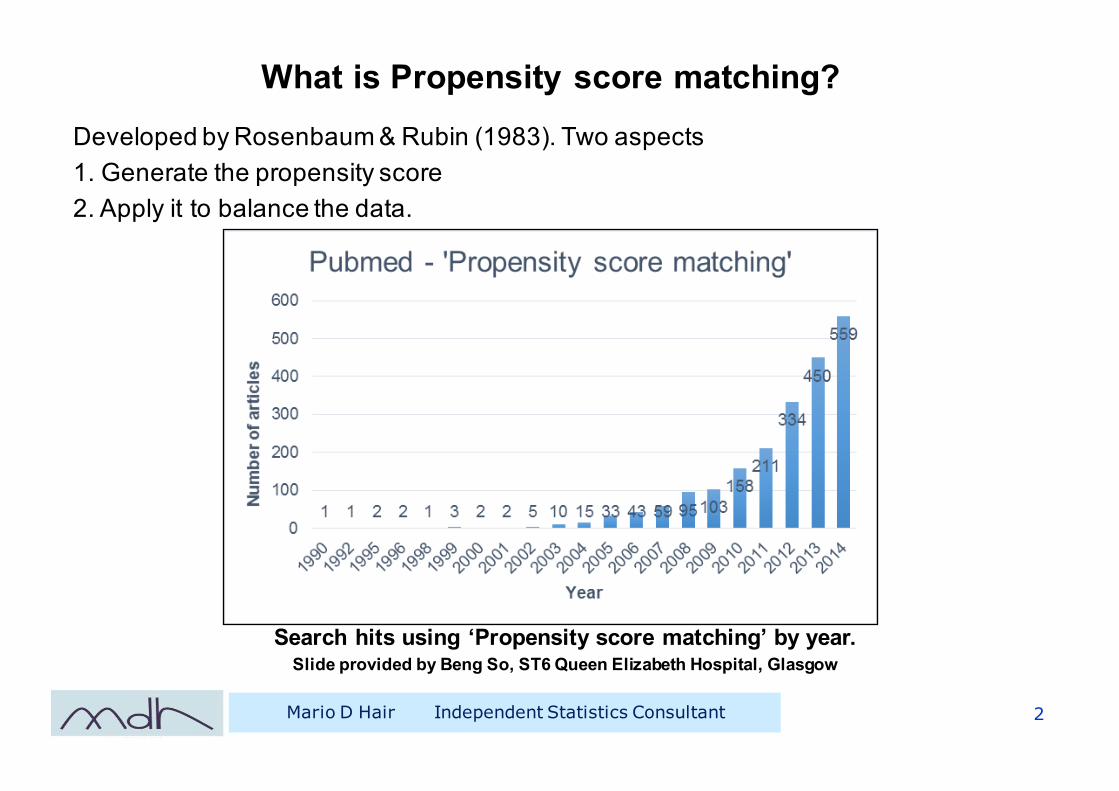
What is Propensity score matching?Developed by Rosenbaum & Rubin (1983). Two aspects1. Generate the propensity score2. Apply it to balance the data.

Search hits using ‘Propensity score matching’ by year. Slide provided by Beng So, ST6 Queen Elizabeth Hospital, Glasgow


What is Propensity score matching?

1. Generate the propensity scoreThe propensity score is the probability (from 0 to 1) of a case being in a particular group based on a given set of covariates. Generally calculated using logistic regression with group (Treatment /Control) as dependent , covariates as independent variables.

Caveats & Limitations• Can only be two groups. If more groups need to analyse them pairwise.• The propensity score is only as good as the predictors used to generate it. • Propensity score not generated for any case with any missing data. • Not interested in any aspect of the logistic model other than the probabilities.

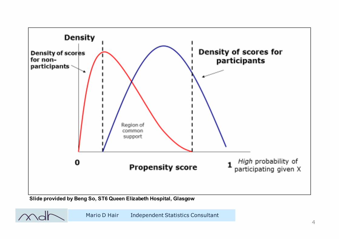
The propensity score is a balancing score: The differences between groups on the covariates condensed down into a single score so if two groups balanced on the propensity score then balanced on all the covariates.


Mario D Hair Independent Statistics Consultant4

Slide provided by Beng So, ST6 Queen Elizabeth Hospital, Glasgow

What is Propensity score matching?

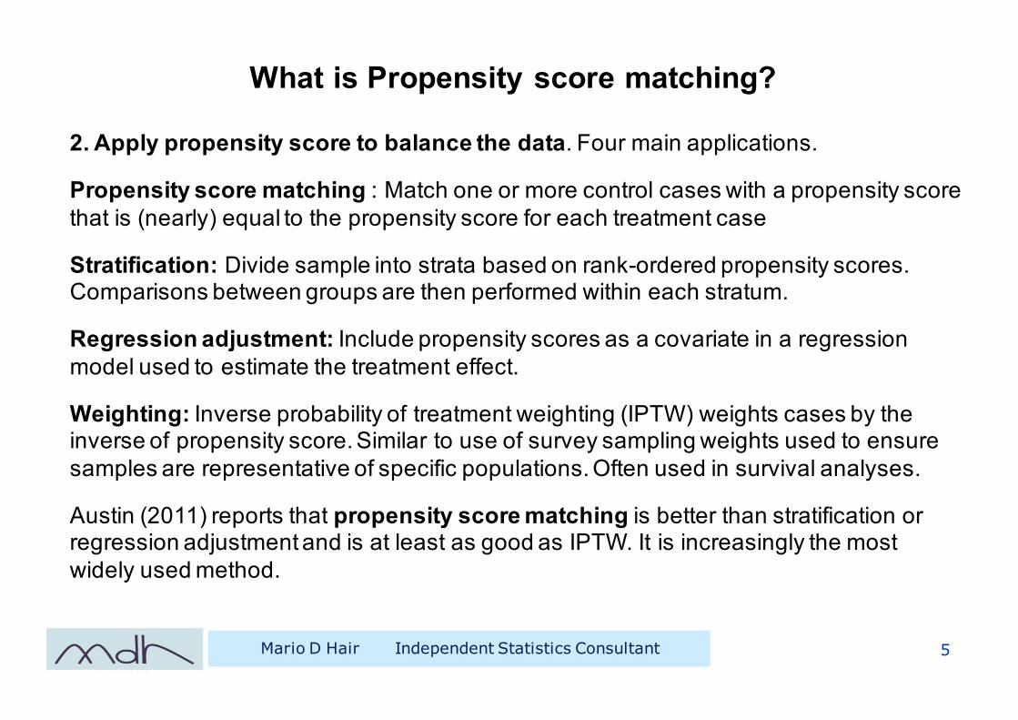
2. Apply propensity score to balance the data. Four main applications.

Propensity score matching : Match one or more control cases with a propensity score that is (nearly) equal to the propensity score for each treatment case

Stratification: Divide sample into strata based on rank-ordered propensity scores. Comparisons between groups are then performed within each stratum.

Regression adjustment: Include propensity scores as a covariate in a regression model used to estimate the treatment effect.

Weighting: Inverse probability of treatment weighting (IPTW) weights cases by the inverse of propensity score. Similar to use of survey sampling weights used to ensure samples are representative of specific populations. Often used in survival analyses.

Austin (2011) reports that propensity score matching is better than stratification or regression adjustment and is at least as good as IPTW. It is increasingly the most widely used method.


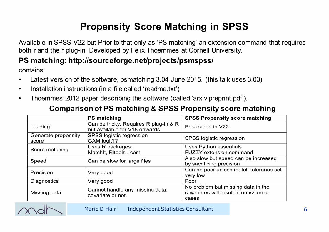
Propensity Score Matching in SPSSAvailable in SPSS V22 but Prior to that only as ‘PS matching’ an extension command that requires both r and the r plug-in. Developed by Felix Thoemmes at Cornell University. PS matching: http://sourceforge.net/projects/psmspss/ contains • Latest version of the software, psmatching 3.04 June 2015. (this talk uses 3.03)• Installation instructions (in a file called ‘readme.txt’) • Thoemmes 2012 paper describing the software (called ‘arxiv preprint.pdf’).

Comparison of PS matching & SPSS Propensity score matching


PS matching SPSS Propensity score matching

Loading Can be tricky. Requires R plug-in & R but available for V18 onwards Pre-loaded in V22

Generate propensity score

SPSS logistic regression GAM logit?? SPSS logistic regression

Score matching Uses R packages: MatchIt, Rltools , cem

Uses Python essentials FUZZY extension command

Speed Can be slow for large files Also slow but speed can be increased by sacrificing precision

Precision Very good Can be poor unless match tolerance set very low

Diagnostics Very good Poor

Missing data Cannot handle any missing data, covariate or not.

No problem but missing data in the covariates will result in omission of cases


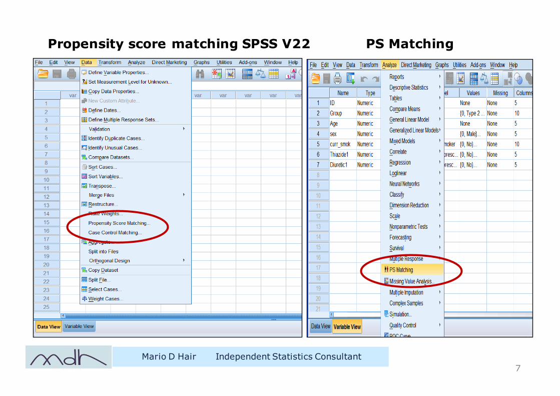
Propensity score matching SPSS V22 PS Matching

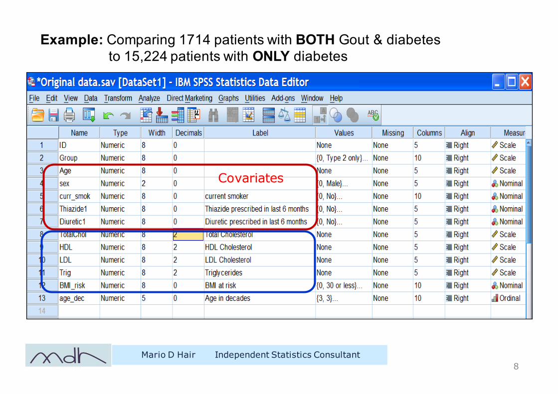
Example: Comparing 1714 patients with BOTH Gout & diabetesto 15,224 patients with ONLY diabetes


Covariates

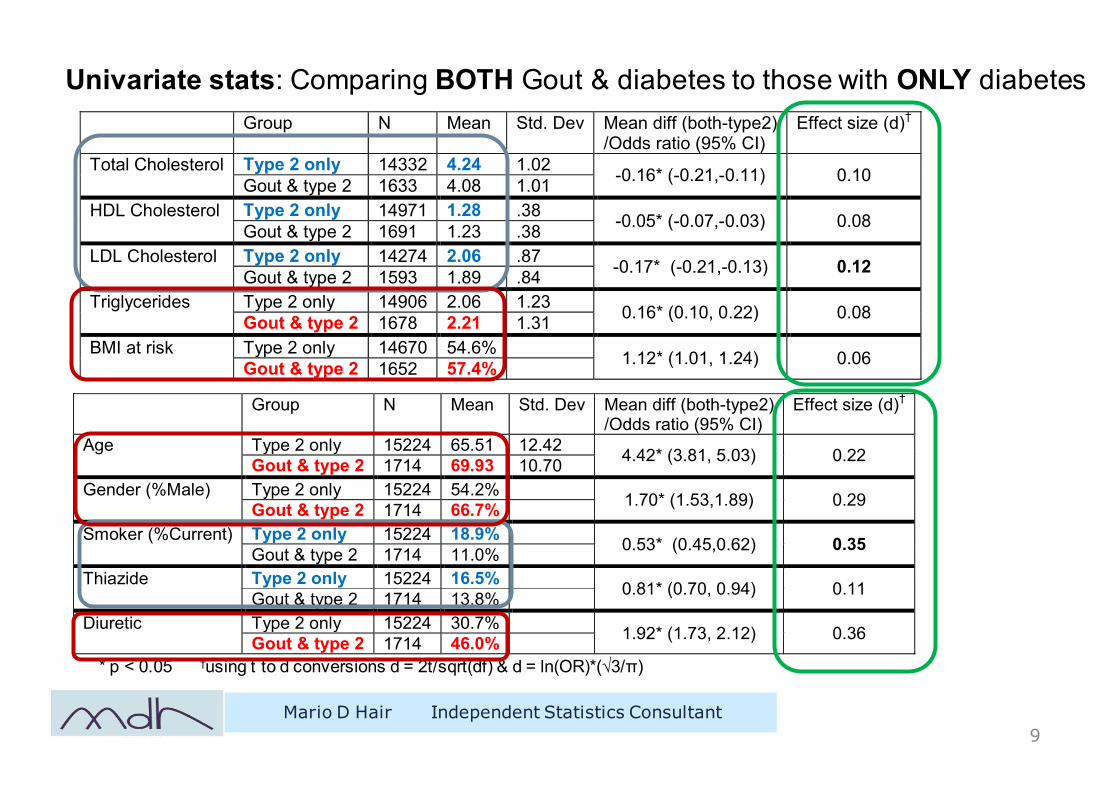
Univariate stats: Comparing BOTH Gout & diabetes to those with ONLY diabetes


Group N Mean Std. Dev Mean diff (both-type2) /Odds ratio (95% CI)

Effect size (d)†

Total Cholesterol Type 2 only 14332 4.24 1.02 -0.16* (-0.21,-0.11) 0.10 Gout & type 2 1633 4.08 1.01 HDL Cholesterol Type 2 only 14971 1.28 .38 -0.05* (-0.07,-0.03) 0.08 Gout & type 2 1691 1.23 .38 LDL Cholesterol Type 2 only 14274 2.06 .87 -0.17* (-0.21,-0.13) 0.12 Gout & type 2 1593 1.89 .84 Triglycerides Type 2 only 14906 2.06 1.23 0.16* (0.10, 0.22) 0.08 Gout & type 2 1678 2.21 1.31 BMI at risk Type 2 only 14670 54.6% 1.12* (1.01, 1.24) 0.06 Gout & type 2 1652 57.4%

* p < 0.05 †using t to d conversions d = 2t/sqrt(df) & d = ln(OR)*(√3/π)

Group N Mean Std. Dev Mean diff (both-type2) /Odds ratio (95% CI)

Effect size (d)†

Age Type 2 only 15224 65.51 12.42 4.42* (3.81, 5.03) 0.22 Gout & type 2 1714 69.93 10.70 Gender (%Male) Type 2 only 15224 54.2% 1.70* (1.53,1.89) 0.29 Gout & type 2 1714 66.7% Smoker (%Current) Type 2 only 15224 18.9% 0.53* (0.45,0.62) 0.35 Gout & type 2 1714 11.0% Thiazide Type 2 only 15224 16.5% 0.81* (0.70, 0.94) 0.11 Gout & type 2 1714 13.8% Diuretic Type 2 only 15224 30.7% 1.92* (1.73, 2.12) 0.36 Gout & type 2 1714 46.0%

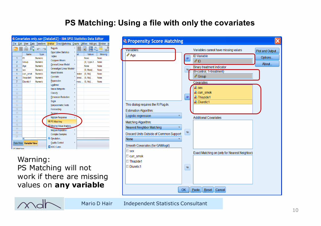
PS Matching: Using a file with only the covariates


Warning:PS Matching will not work if there are missing values on any variable

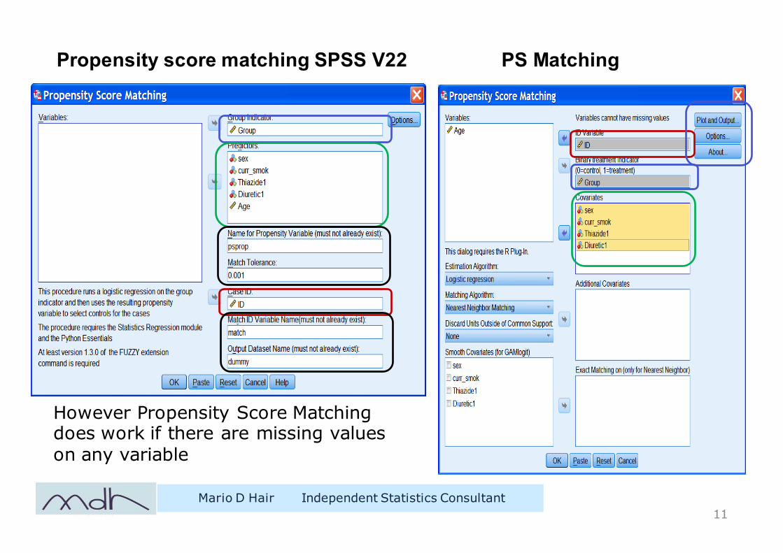
Propensity score matching SPSS V22 PS Matching


However Propensity Score Matching does work if there are missing values on any variable

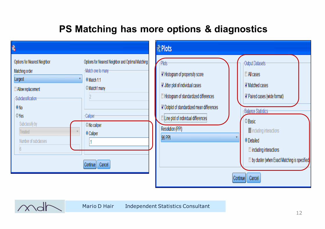
PS Matching has more options & diagnostics


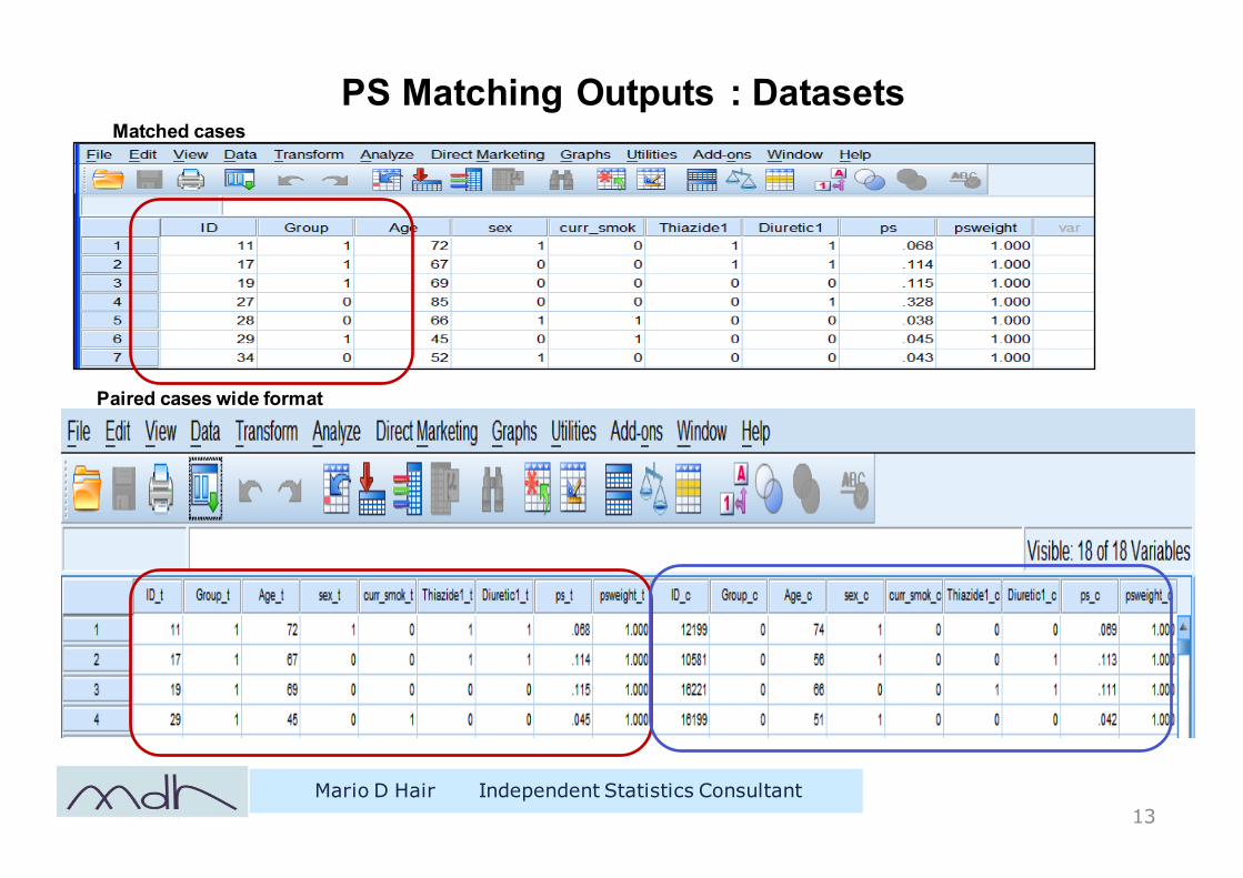
PS Matching Outputs : Datasets


Paired cases wide format

Matched cases

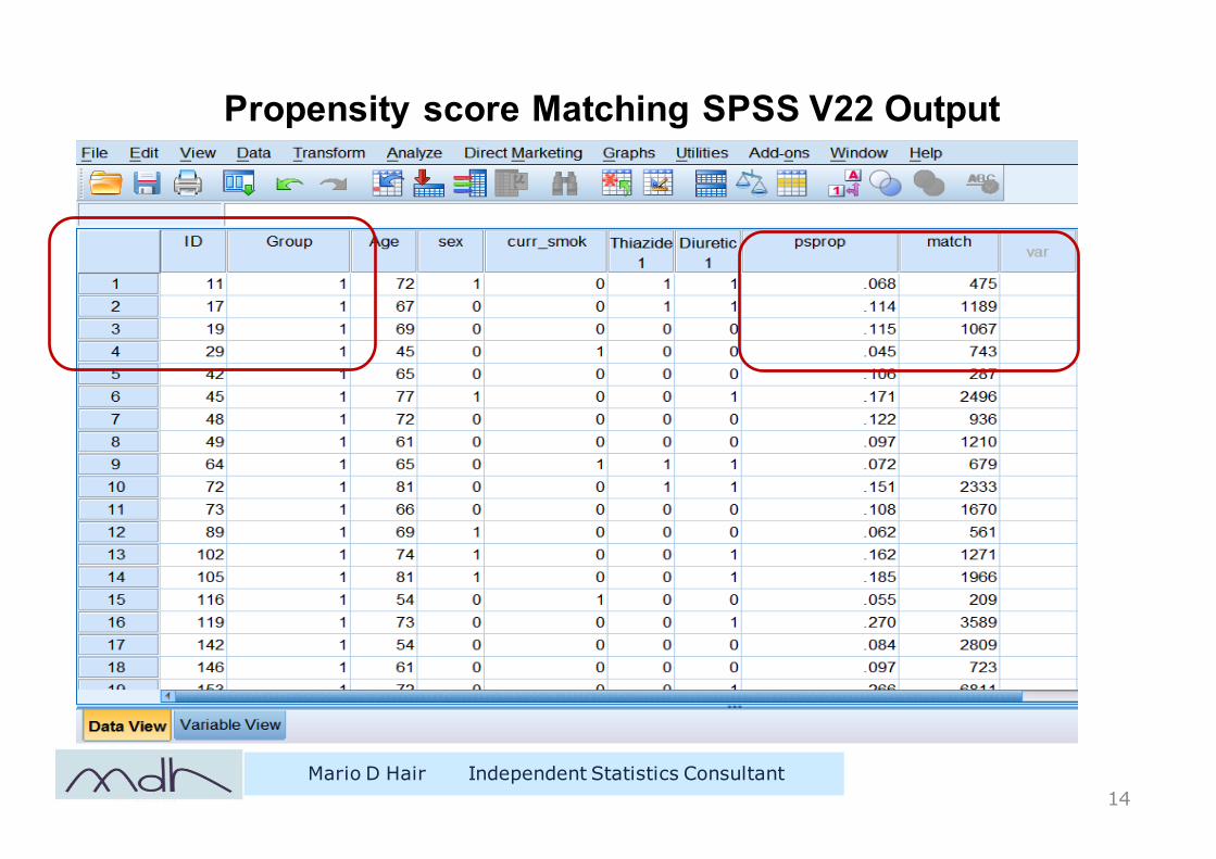
Propensity score Matching SPSS V22 Output


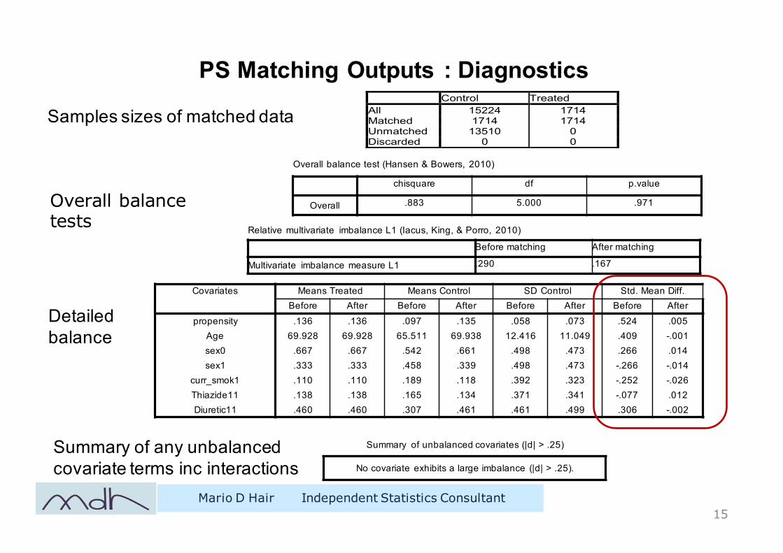
PS Matching Outputs : Diagnostics


Control Treated All 15224 1714 Matched 1714 1714 Unmatched 13510 0 Discarded 0 0

Samples sizes of matched data

Overall balance test (Hansen & Bowers, 2010)

chisquare df p.value

Overall .883 5.000 .971Overall balance tests Relative multivariate imbalance L1 (Iacus, King, & Porro, 2010)

Before matching After matching

Multivariate imbalance measure L1 .290 .167

Covariates Means Treated Means Control SD Control Std. Mean Diff.Before After Before After Before After Before After

propensity .136 .136 .097 .135 .058 .073 .524 .005Age 69.928 69.928 65.511 69.938 12.416 11.049 .409 -.001sex0 .667 .667 .542 .661 .498 .473 .266 .014sex1 .333 .333 .458 .339 .498 .473 -.266 -.014

curr_smok1 .110 .110 .189 .118 .392 .323 -.252 -.026Thiazide11 .138 .138 .165 .134 .371 .341 -.077 .012Diuretic11 .460 .460 .307 .461 .461 .499 .306 -.002

Detailed balance

Summary of unbalanced covariates (|d| > .25)

No covariate exhibits a large imbalance (|d| > .25).

Summary of any unbalanced covariate terms inc interactions

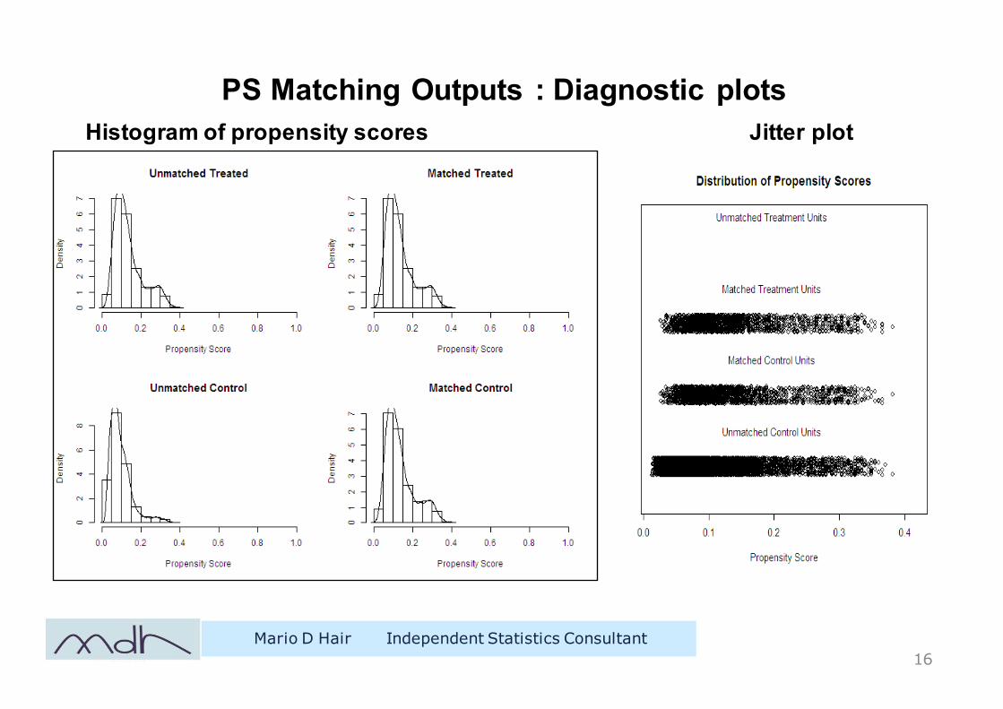
PS Matching Outputs : Diagnostic plots


Histogram of propensity scores Jitter plot

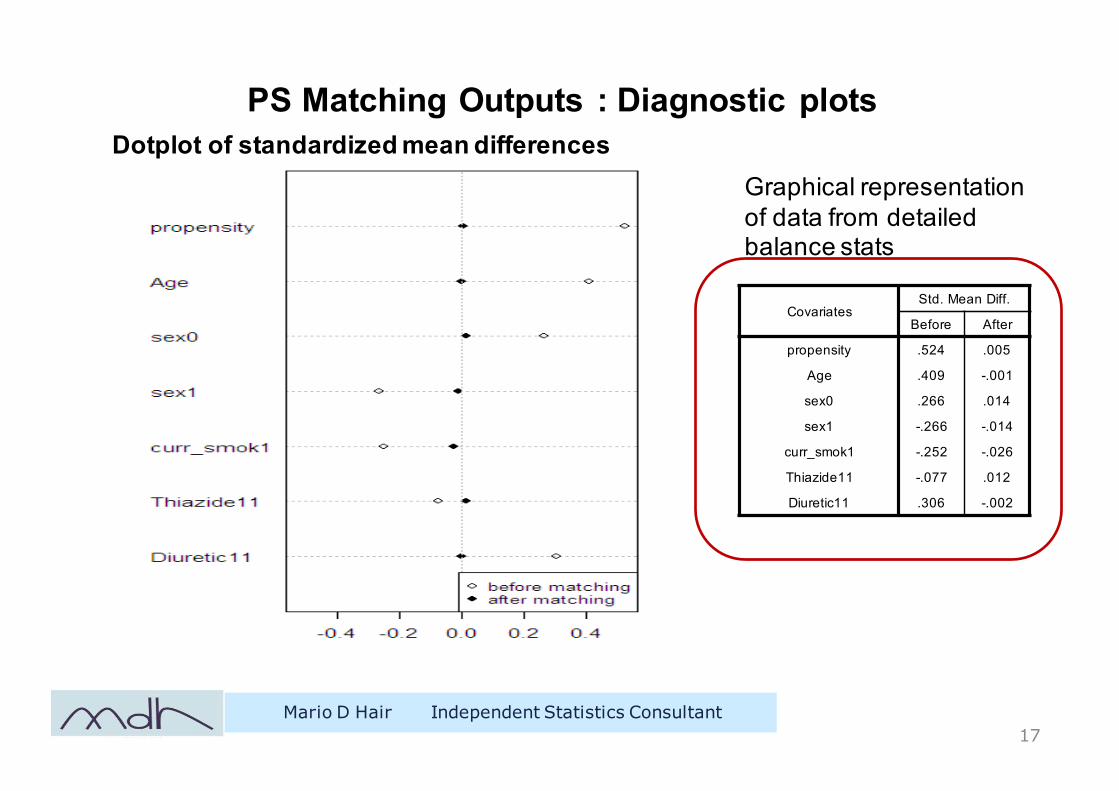
PS Matching Outputs : Diagnostic plots


Dotplot of standardized mean differences

CovariatesStd. Mean Diff.

Before After

propensity .524 .005

Age .409 -.001

sex0 .266 .014

sex1 -.266 -.014

curr_smok1 -.252 -.026

Thiazide11 -.077 .012

Diuretic11 .306 -.002

Graphical representation of data from detailed balance stats

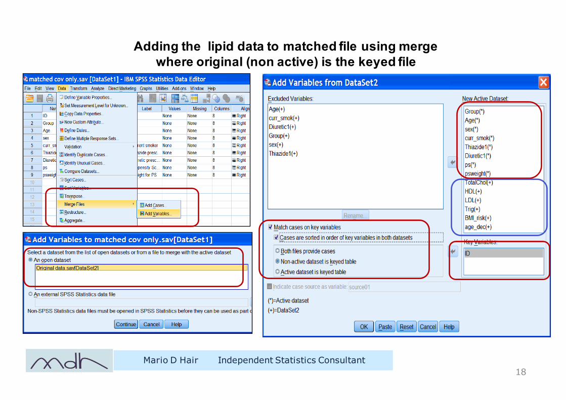
Adding the lipid data to matched file using merge where original (non active) is the keyed file


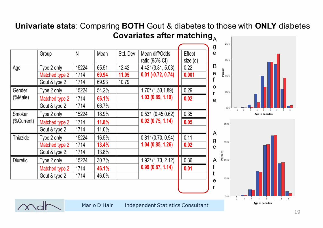
Univariate stats: Comparing BOTH Gout & diabetes to those with ONLY diabetes Covariates after matching


Age

Before

Age

Af ter

Group N Mean Std. Dev Mean diff/Odds ratio (95% CI)

Effect size (d)

Age Type 2 only 15224 65.51 12.42 4.42* (3.81, 5.03) 0.01 (-0.72, 0.74)

0.22 Matched type 2 1714 69.94 11.05 0.001 Gout & type 2 1714 69.93 10.79

Gender (%Male)

Type 2 only 15224 54.2% 1.70* (1.53,1.89) 1.03 (0.89, 1.19)

0.29 Matched type 2 1714 66.1% 0.02 Gout & type 2 1714 66.7%

Smoker (%Current)

Type 2 only 15224 18.9% 0.53* (0.45,0.62) 0.92 (0.75, 1.14)


Thiazide Type 2 only 15224 16.5% 0.81* (0.70, 0.94) 1.04 (0.85, 1.26)


Diuretic Type 2 only 15224 30.7% 1.92* (1.73, 2.12) 0.99 (0.87, 1.14)


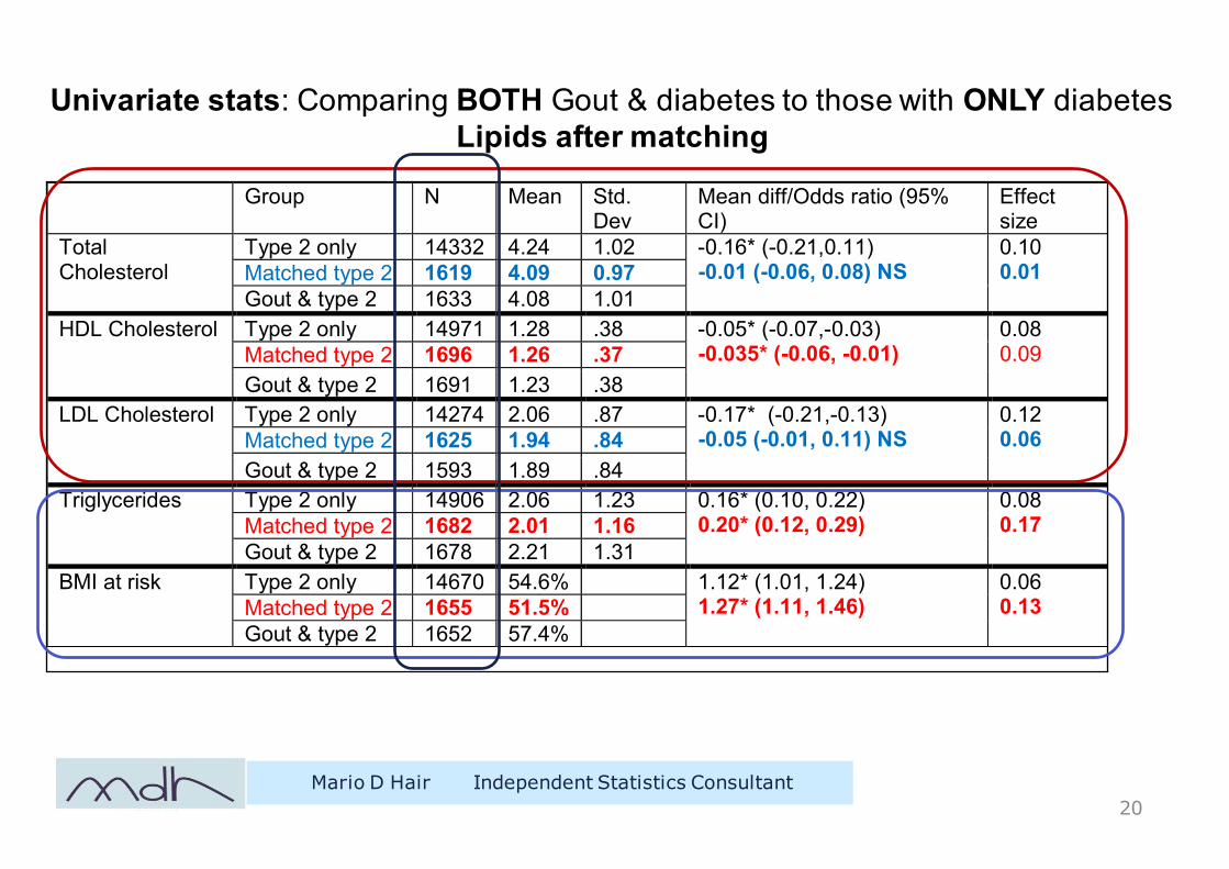
Univariate stats: Comparing BOTH Gout & diabetes to those with ONLY diabetes Lipids after matching


Group N Mean Std. Dev

Mean diff/Odds ratio (95% CI)

Effect size

Total Cholesterol

Type 2 only 14332 4.24 1.02 -0.16* (-0.21,0.11) -0.01 (-0.06, 0.08) NS

0.10 0.01 Matched type 2 1619 4.09 0.97

Gout & type 2 1633 4.08 1.01 HDL Cholesterol Type 2 only 14971 1.28 .38 -0.05* (-0.07,-0.03)

-0.035* (-0.06, -0.01) 0.08 0.09 Matched type 2 1696 1.26 .37

Gout & type 2 1691 1.23 .38 LDL Cholesterol Type 2 only 14274 2.06 .87 -0.17* (-0.21,-0.13)

-0.05 (-0.01, 0.11) NS 0.12 0.06 Matched type 2 1625 1.94 .84

Gout & type 2 1593 1.89 .84 Triglycerides Type 2 only 14906 2.06 1.23 0.16* (0.10, 0.22)

0.20* (0.12, 0.29) 0.08 0.17 Matched type 2 1682 2.01 1.16

Gout & type 2 1678 2.21 1.31 BMI at risk Type 2 only 14670 54.6% 1.12* (1.01, 1.24)

1.27* (1.11, 1.46) 0.06 0.13 Matched type 2 1655 51.5%

Gout & type 2 1652 57.4%

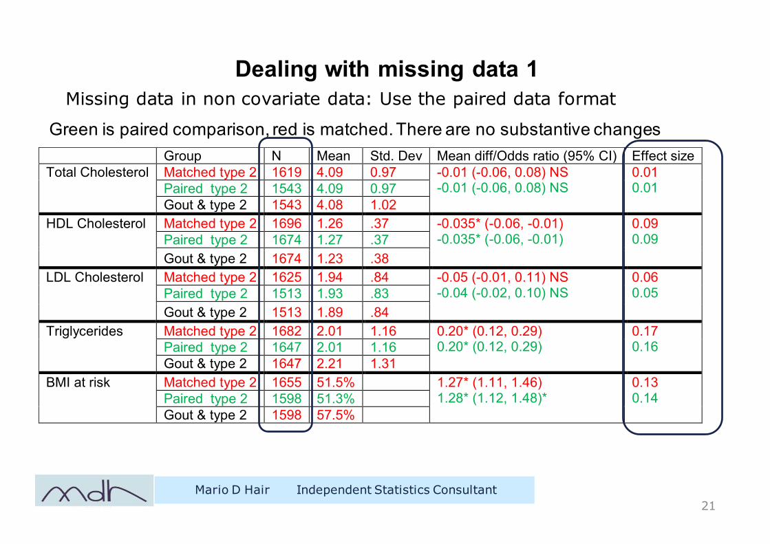
Dealing with missing data 1


Missing data in non covariate data: Use the paired data format

Group N Mean Std. Dev Mean diff/Odds ratio (95% CI) Effect size Total Cholesterol Matched type 2 1619 4.09 0.97 -0.01 (-0.06, 0.08) NS

-0.01 (-0.06, 0.08) NS 0.01 0.01 Paired type 2 1543 4.09 0.97

Gout & type 2 1543 4.08 1.02 HDL Cholesterol Matched type 2 1696 1.26 .37 -0.035* (-0.06, -0.01)

-0.035* (-0.06, -0.01) 0.09 0.09 Paired type 2 1674 1.27 .37

Gout & type 2 1674 1.23 .38 LDL Cholesterol Matched type 2 1625 1.94 .84 -0.05 (-0.01, 0.11) NS

-0.04 (-0.02, 0.10) NS 0.06 0.05 Paired type 2 1513 1.93 .83

Gout & type 2 1513 1.89 .84 Triglycerides Matched type 2 1682 2.01 1.16 0.20* (0.12, 0.29)

0.20* (0.12, 0.29) 0.17 0.16 Paired type 2 1647 2.01 1.16

Gout & type 2 1647 2.21 1.31 BMI at risk Matched type 2 1655 51.5% 1.27* (1.11, 1.46)

1.28* (1.12, 1.48)* 0.13 0.14 Paired type 2 1598 51.3%

Gout & type 2 1598 57.5%

Green is paired comparison, red is matched. There are no substantive changes

Dealing with missing data 2


Missing data in covariates: Use multiple imputation

• Separate creation of propensity scores from the matching

• Run logistic regression on imputed datasets

• Aggregate to get mean (median) propensity score

• Use the aggregate file to do the matching

• Load in the other variables

• Use imputation again if missing data in non-covariates

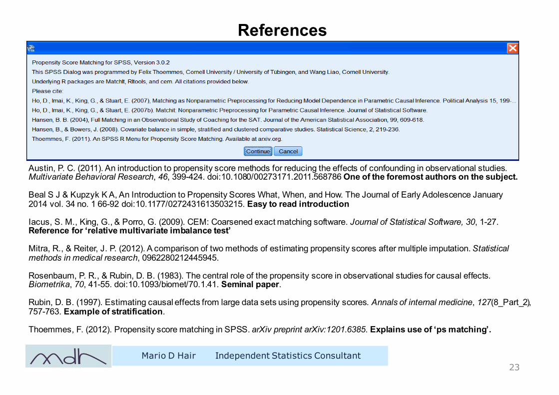
References


Austin, P. C. (2011). An introduction to propensity score methods for reducing the effects of confounding in observational studies. Multivariate Behavioral Research, 46, 399-424. doi:10.1080/00273171.2011.568786 One of the foremost authors on the subject.

Beal S J & Kupzyk K A, An Introduction to Propensity Scores What, When, and How. The Journal of Early Adolescence January 2014 vol. 34 no. 1 66-92 doi:10.1177/0272431613503215. Easy to read introduction

Iacus, S. M., King, G., & Porro, G. (2009). CEM: Coarsened exact matching software. Journal of Statistical Software, 30, 1-27. Reference for ‘relative multivariate imbalance test’

Mitra, R., & Reiter, J. P. (2012). A comparison of two methods of estimating propensity scores after multiple imputation.Statistical methods in medical research, 0962280212445945.

Rosenbaum, P. R., & Rubin, D. B. (1983). The central role of the propensity score in observational studies for causal effects. Biometrika, 70, 41-55. doi:10.1093/biomet/70.1.41. Seminal paper.

Rubin, D. B. (1997). Estimating causal effects from large data sets using propensity scores. Annals of internal medicine, 127(8_Part_2), 757-763. Example of stratification.

Thoemmes, F. (2012). Propensity score matching in SPSS. arXiv preprint arXiv:1201.6385. Explains use of ‘ps matching’.

Propensity Score Matching in SPSS:How to turn an Audit into a RCT

Outline• What is Propensity score matching?• Propensity Score Matching in SPSS• Example: Comparing patients with both Gout & diabetes to those with diabetes only• Dealing with missing data

Thank you: Questions?


Mario D Hair Independent Statistics Consultant

Propensity+Score+Matching+in+SPSS: … ·...

Documents

Transcript of Propensity+Score+Matching+in+SPSS: … ·...