Propagation Terminal Design and Measurements

National Aeronautics and Space AdministrationGlenn Research Center at Lewis Field

November 16, 2015

Keeping the universe connected.

Propagation Terminal Design and Measurements

James Nessel

NASA Glenn Research CenterAdvanced High Frequency Branch

Goals of this Presentation

• To provide the motivation behind conducting propagation measurements.

• To understand the system design for beacon receivers (i.e., propagation terminals) and the types of measurements performed.

• To provide examples as to how propagation data can be/has been used for defining requirements for a satellite communications system.

2

Relevance/ImpactWhy do we need Propagation Data?

Ground StationAntenna Size

System Temperature

SpacecraftAntenna Size

Transmit PowerGimbal Requirements

Propagation ChannelRain Attenuation

Gaseous AbsorptionDepolarizationFree Space Loss

It is well understood that the largest uncertainty in Earth‐space communications system design lies in the impact of the stochastic atmospheric channel on propagating electromagnetic waves.

Proper characterization of the atmosphere is necessary to mitigate risk and reduce lifetime costs through the optimal design of the space and ground segment.

As NASA continues to move towards Ka‐band operations (currently) and millimeter wave/optical frequencies (future), the need for this data is becoming more and more evident and requested by system designers.

3

Primary Objectives of Propagation Data Collection: • To reduce mission risk and mission costs by ensuring optimal design of SATCOM systems

• To improve predictions of global propagation models

Relevance/ImpactWhat Propagation Data Helps Support

4Guam (SN)Guam (SN)

Ka-band (Next Gen.)

Next Generation Space Network

White Sands Complex (SN)

Ka-Band, Optical, or V/W-band (Next Gen.)

Svalbard (NEN)Alaska (NEN)

Ku-Band (Current)

S/X-band (Current)

LEO Spacecraft

Goldstone (DSN)

Ka-band Uplink Array (Next Gen.)

GRC/GSFC data collection inGuam is providing shortbaseline site diversity data forpractical implementation of Ka‐band in tropical environments.

GRC/GSFC data collection inSvalbard is providing criticalcharacterization of Ka‐bandperformance at low elevation anglepolar sites for NEN upgrades.

As NASA Networks continue their current transitionto Ka‐band and future transition to higher frequencyallocations (e.g., for the next generation SBR), GRCpropagation data collection will influence SCaNNetwork architecture design through optimalunderstanding of system margin requirements andcompensation of existing assets to enhance Networkoperational availability

GRC/JPL data collection at DSN sitesare providing characterization ofturbulence effects for the practicalimplementation of Ka‐band uplinkarrays for DSN upgrades.GRC/GSFC/AFRL data collection

in White Sands is providingavailability measurements ofKa/Q/V/W‐band potential for RFSpace‐Ground Links.

PROPAGATION STUDIESTask History

5

RF Propagation Program HistoryAdvanced Communications Technology Satellite (ACTS)

6

GRC opened up the Ka band spectrum through propagation characterization in the 1990’s through the AdvancedCommunications Technology Satellite (ACTS) program.

Current NASA Network Characterization Sites

In the post‐ACTS era, NASA propagation activities have primarily focused on site characterization of NASA operational networks throughout the world.

7

Propagation Data Collected by NASA

8

Location Satellite Used Frequency: Station Years Measurements Performed/Lessons Learned

Fairbanks, Alaska ACTS 20.2 GHz : 5 yrs.27.5 GHz : 5 yrs.

Rain AttenuationScintillation

British Columbia, Canada ACTS 20.2 GHz : 5 yrs.27.5 GHz : 5 yrs.

Rain AttenuationScintillation effects

Fort Collins, Colorado ACTS 20.2 GHz : 5 yrs.27.5 GHz : 5 yrs.

Rain and snow effectsPolarimetric radar

Tampa, Florida ACTS 20.2 GHz : 5 yrs.27.5 GHz : 5 yrs.

Rain Attenuation (Subtropical Zone)Site Diversity

Norman, Oklahoma ACTS 20.2 GHz : 5 yrs.27.5 GHz : 5 yrs.

Rain AttenuationScintillation

Snow on AntennaClarksburg, MD ACTS 20.2 GHz : 5 yrs.

27.5 GHz : 5 yrs.Rain Attenuation

ScintillationAshburn, VA ACTS 20.2 GHz : ~1 yr. Depolarization

Humacao, Puerto Rico UFO 09 20.7 GHz : 1.5 yrs. Rain Attenuation (Tropical Zone)

Goldstone, California ANIK F2CIEL 2

20.2 GHz : 7 yrs.12.45 GHz: 4 yrs.

Phase DecorrelationTotal Attenuation

Las Cruses, New Mexico ANIK F2 20.2 GHz : 12 yrs.27.5 GHz : 5 yrs.

Phase Decorrelation (6 yrs.)Total Attenuation (12 yrs.)Atmospheric Profiles (3 yrs.)

Guam, USA UFO 08 20.7 GHz : 5 yrs.Phase Decorrelation

Rain Attenuation (Tropical Zone)Site Diversity

Canberra, Australia OPTUS D3 11.95 GHz: 3 yrs. Phase Decorrelation

Madrid, Spain EUTELSAT 9A 11.95 GHz: 1 yr. Phase Decorrelation

Svalbard, Norway N/A 22.234 GHz: 3 yrs.26.5 GHz: 3 yrs.

Gaseous Absorption (Low Elevation Angles)Cloud Attenuation

Milan, Italy Alphasat 19.7 GHz: 1 yr.39.4 GHz: 1 yr. Total Attenuation

PROPAGATION EXPERIMENT REQUIREMENTS

9

Atmospheric Propagation Effects at Ka‐band and Above

• Rain, rain, go away!

10

, ,

,

,

, ,

Characterization Techniques

11

Desired Measurement

Reason for Measurement Technology Pros/Cons

Attenuation Characterization of link margin availability as a result of losses through the atmosphere.

Dominant atmospheric mechanism for defining system link

Beacon Receiver • Provides DIRECT power loss measurement ofatmosphere in all conditions (clear sky, cloudy, rain,snow, etc.)

• Difficulty in scaling results from one frequency toanother, unless known site‐dependent scaling factor dataexists.

• Requires source signal

Radiometer • INDIRECT power loss measurement of atmosphere inonly clear sky/cloudy conditions.

• In combination with Beacon Receiver, provides referenceattenuation level

• Does not require source signal

Brightness Temperature Desire to determine atmospheric noise temperature contribution to low receiver noise systems (high G, low T systems)

Radiometer

Phase Desire arraying capability at a particular site for link margin availability

Interferometer • Provides DIRECT measurement of atmospheric‐inducedphase fluctuations

• Requires source signal (beacon, quasar, downlink)

Water Vapor Radiometer • INDIRECT measurement of atmospheric phasefluctuations

• Reliant on local radiosonde database and models toextract phase from water vapor content

• Limited to longer integration times (>2 sec)• Does not require source signal

Depolarization Provide double the data capacity through us of dual polarization receive/ transmit

Beacon Receiver

Scintillation Important for low elevation angle links Beacon Receiver

Goldstone

12

Step 1: Identify Signals of Opportunity

White Sands

KaSAT

Fairbanks

AlphasatAnik F2

KaSAT: 19.68 GHz Beacon

Anik F2: 20.199 GHz Beacon

Alphasat: 19.701 GHz Beacon39.402 GHz Beacon

Thor 7

Thor 7: 20.198 GHz Beacon

Svalbard

Milan

EdinburghCleveland

39.402 GHz0.008 m26.50 dBW

38600 km

0.5 dB0.0 dB0.0 dB0.0 dB

216.08 dB

Antenna Diameter 0.6 mIllumination Taper Factor 70 degHalf Power Beamwidth 0.888 degAntenna Efficiency 60 %Antenna Gain 45.66 dBNoise Temperature Contributions:

Cosmic Background Noise Temperature 2.8 KAtmosphere Physical Temperature 290 KAntenna Noise Temperature (Clear Sky) 34.03 KAntenna Noise Temperature (Rain) 34.03 KReceiver Noise Temperature 800 K

System Temperature 834.03 K29.21 dBK

Boltzmann's Constant ‐228.60 dBW/K·HzNoise Spectral Density ‐199.39 dBGain over Noise Temperature Ratio (G/T) 16.44 dB/KReceived Carrier Power (C) ‐144.43 dBWCarrier to Noise Density (C/N0) 54.96 dBHz

Pointing LossPolarization LossFree Space Loss

Receive Antenna Parameters

Transmitter Receiver Range

Gaseous Absorption LossRain Attenuation

Effective Isotropic Radiated Power (EIRP)Propagation Channel Parameters

Parameter User Inputs CalculatedFrequency of OperationWavelength

39.402 GHz0.008 m26.50 dBW

38600 km

0.5 dB0.0 dB0.0 dB0.0 dB

216.08 dB

Antenna Diameter 0.6 mIllumination Taper Factor 70 degHalf Power Beamwidth 0.888 degAntenna Efficiency 60 %Antenna Gain 45.66 dBNoise Temperature Contributions:

Cosmic Background Noise Temperature 2.8 KAtmosphere Physical Temperature 290 KAntenna Noise Temperature (Clear Sky) 34.03 KAntenna Noise Temperature (Rain) 34.03 KReceiver Noise Temperature 800 K

System Temperature 834.03 K29.21 dBK

Boltzmann's Constant ‐228.60 dBW/K·HzNoise Spectral Density ‐199.39 dBGain over Noise Temperature Ratio (G/T) 16.44 dB/KReceived Carrier Power (C) ‐144.43 dBWCarrier to Noise Density (C/N0) 54.96 dBHz

Pointing LossPolarization LossFree Space Loss

Receive Antenna Parameters

Transmitter Receiver Range

Gaseous Absorption LossRain Attenuation

Effective Isotropic Radiated Power (EIRP)Propagation Channel Parameters

Parameter User Inputs CalculatedFrequency of OperationWavelength

Step 2: Link Budget EstimatesExample: Alphasat Q‐band Beacon

13

Obtained from Satellite Operator

Estimates from Models/Experience

4

End Result: Provides dynamic range estimate of receiver

.

55 10 1035

~ ‐115 dBm power level at antenna flange

Can adjust antenna size to obtain desired dynamic range… Trades: Tracking Requirements

Receiver Noise Temperature primarily determined by LNA performance…Good LNA: ~ 600KNot So Good LNA: ~ 1000‐1200K

Parameters fixed by virtue of experimental setup

Dominant parameter to define dynamic range performance of receiver

Parameter determined from system design (limited improvement)

Step 3: System Design

14

To DAQ…

Low Noise Amplifier (LNA)

IF Amp~~~Filter

~

Mixer

Local Oscillator (LO)

The role of the propagation terminal hardware is simply to provide a means to convert the receive beacon frequency to a more manageable intermediate frequency (IF) for digitizing…

Losses before LNA can dominate system noise

Antenna size will determine maximum receive signal strength

LNA amplifies signal and noise, as well as introduces additional noise

Desire low phase noise for frequency stability

DownconverterSubsystem

Spectrum Representation

RF leakage

LO leakage

IF

Mixer multiplies input frequencies to generate IF frequency

Bandpass/Lowpass filters to remove spurious frequencies

~~~Filter

Following downconversion, is simply a matter of ensuring signal level range is sufficient enough for digitizer…

TRx =

Step 3: System Noise Temperature

15

~

~~~

Pflange = -115 dBmN0 = -170 dBm/HzC/N0 = 55 dB/Hz

OMT

L = 1 dB

LNA

G = 35 dBNF = 2.7 dB

Mixer

20.129 GHz LO

L = 9 dB

LPF

L = 1 dB

~~~BPF

L = 1.5 dB

IF Amp

G = 29 dBNF = 2.9 dB

~ 10 MHz REF

To DAQ…~~~BPF

~

Mixer

19.203 GHz LO

L = 1 dB L = 10 dB

Splitter

From IF Box…

Pout = -74.5 dBm

681.7 K

1 1 1 1 …

365.1 K 679.8 K 680.6 K

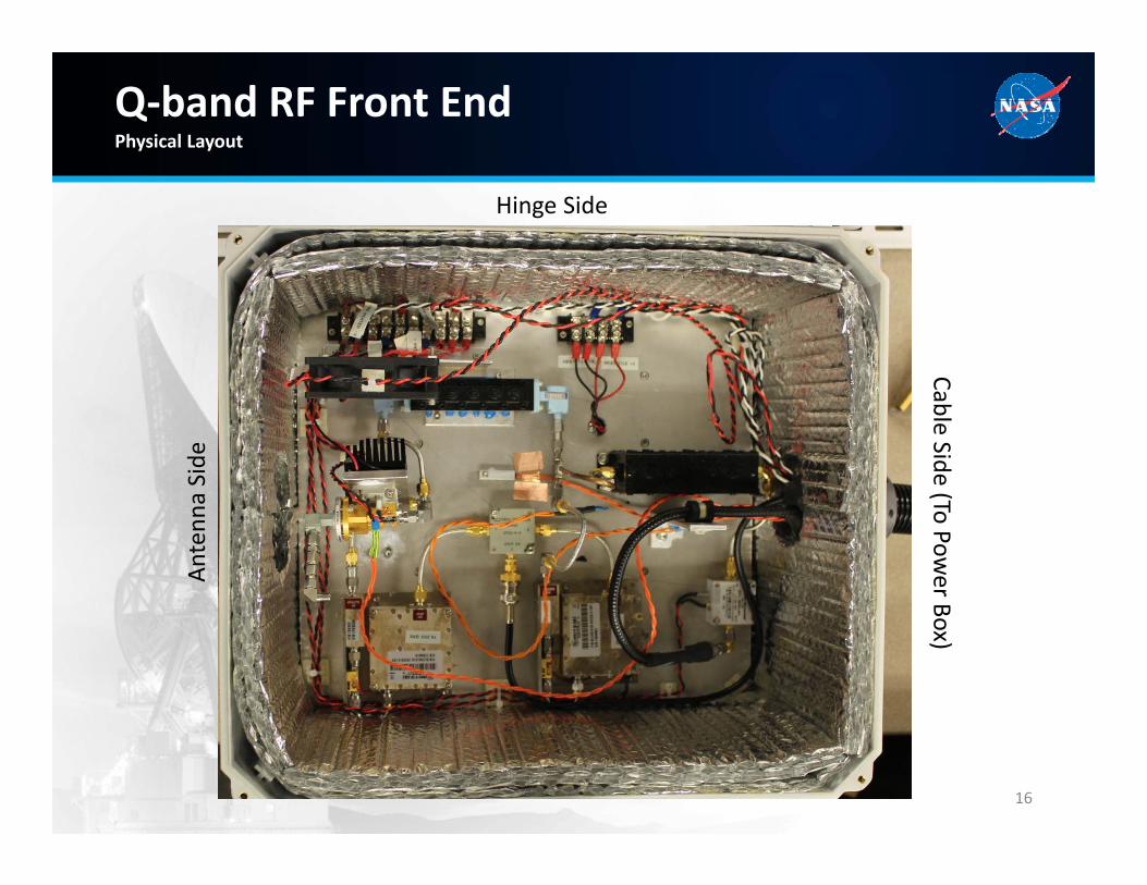
Q‐band RF Front EndPhysical Layout

16

Hinge SideAn

tenn

a Side

Cable Side (To Power Box)

DIGITAL SIGNAL PROCESSING

17

Thewell‐knownNyquist‐ShannonSamplingTheoremstatesthatacontinuous‐timefunctionmustbesampledatarateofatleast2f0 Hz,wheref0 isthehighestfrequencycomponentofthesignal(i.e.asamplingrateof2f0 Hzwillensurethatnoaliasingoccurs).

f0

2f0

National Aeronautics and Space Administration www.nasa.gov 18

Nyquist‐Shannon

Frequency Detection

Detecting the measured frequency of the beacon can be done easily with an FFT, but there are much more accurate

alternatives.

National Aeronautics and Space Administration

www.nasa.gov 19

FFT Peak Search

• The FFT can be used to easily estimate the frequency of a signal by finding the peak bin, but it has a resolution is defined by (where fs is the sampling frequency of the signal and N is the number of points) – this is the distance between two points in the FFT, and thus the finest measurement of frequency we can make by doing a simple peak search.

• In other words, while the actual signal frequency can vary continuously between and 1 , the bins of the FFT are discrete integer multiples of .

Therefore, if we want a fine resolution that can accurately measure frequency, we are forced to choose fs and N such that is very small.


www.nasa.gov 20

1

Binn Binn+1

… …

Whenthefrequencyofasignalfallsexactlyintoabinfrequency,thatbinwillcontainallofthepowerofthesignal.Inallothercases,thepowerofthesignalwillalsobespreadintomultiplenearbybins.

Theworstcasescenariooccurswhenthesignalfrequencyishalfwaybetweentwobinfrequencies,inwhichcasethetwobinsoneithersidewillhavethesameamountofpower(inotherwords,therewillbetwomatchingpeaks).

f0 = Bin Frequency f0 = Half Bin Frequency

Signal Frequency, f0 Signal Frequency, f0


PeakBinMagnitude/Power

However,justdoingasimplepeaksearchignoresotherinformationthattheFFTprovides.

Bin Frequency vs. Half‐Bin Frequency


www.nasa.gov 22

4.54 4.542 4.544 4.546 4.548 4.55 4.552 4.554 4.556 4.558 4.56

x 105

0.05

0.1

0.15

0.2FFT

Frequency

|Y(f)

| 2

4.54 4.542 4.544 4.546 4.548 4.55 4.552 4.554 4.556 4.558 4.56

x 105

0.1

0.2

0.3

0.4

0.5FFT

Frequency

|Y(f)

| 2

Ifweareonlyconsideringthepowerinthepeakbin,weobserveascallopingeffect: thepowerquicklydropsoffwhenwemoveawayfromabinfrequency,thencomesbackupagainaswestartapproachinganotherbinfrequency.

However,ifwealsoconsider±1binoneithersideofthepeak(red),or±2(green)or±5(blue),thescallopingeffectisgreatlymitigated,andwecaptureamajorityofthesignalpower.


Scalloping

455.0 455.1 455.2 455.3 455.4 455.5-8

-7

-6

-5

-4

-3

-2

Input Signal Frequency (kHz)

Pow

er (d

BW

)

Power in FFT Bins - Positive Frequencies Only, -3dBW Input(fs = 3276.8 kHz, N = 32768, fs/N = 100)

Peak BinPeak 1Peak 2Peak 5All Positive Frequencies

Frequency Estimates and IQ Power


www.nasa.gov 24

AtahighSNRof10dB(asexpected)allmethodsotherthantheFFTperformedwell,trackingthefrequencyasitvariedfromexactlyonebinfrequencytothenext.

TheestimatorsalsoeliminatethescallopingthatoccursintherelativepoweroftheIQreceiverifjusttheFFTPeakisused.

10 20 30 40 50 60 70 80 90 100

454.95

454.96

454.97

454.98

454.99

455

455.01

455.02

455.03

455.04

Distance Between Bins [%]

Freq

uenc

y [H

z]

Frequency Estimation fs = 4550; N = 65536; fs/N = 0.069427; SNR = 10

f0 = [454.9583 .... 455.0278]

10 20 30 40 50 60 70 80 90 100-8

-7

-6

-5

-4

-3

-2

-1

0


Rel

ativ

e P

ower

[dB

]

IQ Receiver

FFT PeakQuinn-FernandesQuinn-Fernandes-NesselQuinnJacobsenMacleodBunemanActual Frequency

FFT PeakQuinn-FernandesQuinn-Fernandes-NesselQuinnJacobsenMacleodBuneman



www.nasa.gov 25

WiththeSNRdecreasedto‐10dB,morenoiseisapparentinthefrequencyestimations,buttheycontinuetotrackthefrequencylinearlyandavoidscallopingintheIQreceiverpower.

Buneman inparticularbeginstoexhibitanoisierestimatenearthebinfrequencies(attheedges),whereastheotherestimatesaremoreconsistent.

10 20 30 40 50 60 70 80 90 100

454.95

454.96

454.97

454.98

454.99

455

455.01

455.02

455.03

455.04


Freq

uenc

y [H

z]

Frequency Estimation fs = 4550; N = 65536; fs/N = 0.069427; SNR = -10

f0 = [454.9583 .... 455.0278]

10 20 30 40 50 60 70 80 90 100-8

-7

-6

-5

-4

-3

-2

-1

0


Rel

ativ

e P

ower

[dB

]

IQ Receiver





www.nasa.gov 26

At‐20dBSNR,thenoiseissignificant,buttheestimatorsarestillabletoperform.

TheFFTbeginstooscillatearoundthehalfwaypointbecause,whentherearetwopeaksverysimilarinmagnitude,thenoiseislargeenoughtomakeeitheronethemaximum.

10 20 30 40 50 60 70 80 90 100

454.95

454.96

454.97

454.98

454.99

455

455.01

455.02

455.03

455.04


Freq

uenc

y [H

z]

Frequency Estimation fs = 4550; N = 65536; fs/N = 0.069427; SNR = -20

f0 = [454.9583 .... 455.0278]

10 20 30 40 50 60 70 80 90 100-8

-7

-6

-5

-4

-3

-2

-1

0


Rel

ativ

e P

ower

[dB

]

IQ Receiver



RMS Error vs. SNR


www.nasa.gov 27

WithSNRvaryingfrom‐30to+10dB,eachalgorithm’serrorwithrespecttotheactualfrequency(RMS)isplottedonasemi‐logscaleabove.

Allsixmethodsconsidered(excludingtheFFT)exhibitanexponentialincreaseinRMSerrorastheSNRdecreases.Atapproximately‐24dBSNR,thenoiseatanypointinthespectrummayexceedthepeakoftheFFT,andmostofthemethodsthereforebecomeunabletotrackthefrequency.Quinn‐Fernandes‐Nesselmanagestosurvivebelowthispointbecauseoftheaprioriinformationitisgivenonwheretolookforthepeak.

-30 -25 -20 -15 -10 -5 0 5 10

10-2

10-1

100

SNR [dB]

RM

S (D

evia

tion

from

Act

ual F

requ

ency

) [H

z]RMS (Deviation from Actual Frequency) vs. SNR

fs = 4550; N = 65536; fs/N = 0.069427 f0 = [454.9583 .... 455.0278]


DATA PRODUCTS

28

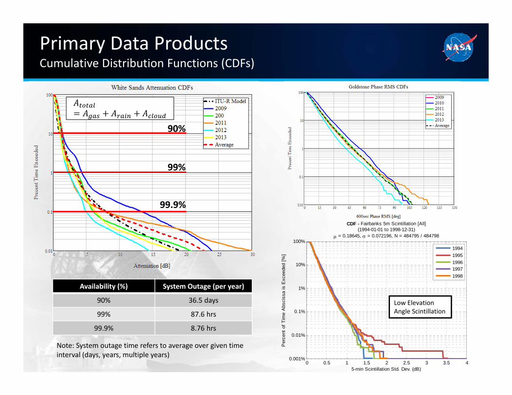
Primary Data ProductsCumulative Distribution Functions (CDFs)

290 0.5 1 1.5 2 2.5 3 3.5 4

0.001%

0.01%

0.1%

1%

10%

100%

5-min Scintillation Std. Dev. (dB)

Per

cent

of T

ime

Abs

ciss

a is

Exc

eede

d [%

]

CDF - Fairbanks 5m Scintillation [All](1994-01-01 to 1998-12-31)

= 0.18645, = 0.072196, N = 484795 / 484798

19941995199619971998

Low Elevation Angle Scintillation

90%

99%

99.9%

Availability (%) System Outage (per year)

90% 36.5 days

99% 87.6 hrs

99.9% 8.76 hrs

Note: System outage time refers to average over given time interval (days, years, multiple years)

Example Higher Order Data Products

30

Fade Duration

• System outage and unavailability: store/forward requirements

• Sharing of the system resource: dynamic reassignment of system

• System coding and modulation: FEC, optimal modulation schemes

Fade Slope

• Fade Mitigation Techniques• Adaptive/Cognitive Systems• Can provide short‐term

statistical prediction

Interannual Variability

• Fade Mitigation Techniques• Seasonal Statistics• Metric for design confidence

level (i.e., probability of exceeding exceedence levels)

Where Does this Data Go?System Design Infusion Path

31

Mission Designers

SATCOM Industry

Other Government Agencies

International Space Agencies

JPL (DSN)

GSFC (NEN/SN)

Other NASA Network Users

International Telecommunications Union

Improve Global Maps/Models

Propagation Data

Attenuation Statistics

Phase Statistics

Second Order Statistics

Atmospheric Models

PROPAGATION DATA FOR MISSION DESIGN

32

Case Study #1Solar Dynamic Observatory (SDO)

• Values used in SDO Downlink Margin Calculation (based on model)

• Design Goal: 99% Availability (87.6 hrs/yr outage)

At 4.06 dB link margin: 99.6% (35 hrs/yr outage)

At 7.90 dB link margin: 99.88%(10.5 hrs/yr outage)

33

3.75 dB

1.36 dB

Atmospheric Loss* 4.06 dB

Margin 3.84 dB

Total Margin 7.90 dB

* model based on worst case elevation angle conditions and did not account for inclined orbit

• Final SDO Architecture utilizes 2 ground station antennas for site diversity (STGT/WSGT, 3km separation distance)

• Analysis for Site Diversity Architecture

– Conclusions: Diversity gain, on average, improves link margin by < 1dB (due to site geometry and average rain conditions)

Results from System Availability Analysis• Over 5 year timespan…

– 615.2 min. of system outage related to weather

– Over 200 mins of downtime due to both dishes being completely full of snow (not modeled in determining atmospheric‐related outages)

34

Case Study #1Solar Dynamic Observatory (SDO)

Margin Measurement Model Actual

Architecture Single Site Diversity Sites Single Site Diversity Sites Diversity Sites

2.24 dB 99.0% 99.45% 97.5% 98.5%* ‐‐

3.75 dB 99.5% 99.6%* 99.0% 99.45% ‐‐

7.90 dB 99.88% 99.92%* 99.7% 99.78%* 99.98%

* Values not available…estimates of availability based on diversity gain estimates

35

From ITU‐R 618‐11: Earth‐Space Link DesignFor non‐geostationary systems, where the elevation angle is varying, the link availability for a single satellite can be calculated in the following way1. Calculate the minimum and maximum elevation

angles at which the system will be expected to operate

2. Divide the operational range of angles into small increments (e.g. 5 bins)

3. Calculate the percentage of time that the satellite is visible as a function of elevation angle in each increment

4. For a given propagation impairment level, find the time percentage that the level is exceeded for each elevation angle increment

5. For each elevation angle increment, multiply the results of (3) and (4) and divide by 100, giving the time percentage that the impairment level is exceeded at this elevation angle

6. Sum the time percentage values obtained in (5) to arrive at the total system time percentage that the impairment level is exceeded

PDF of Elevation Angles

At 99%, range of attenuation from 1.2dB – 12dB over elevation angles

Case Study #2Joint Polar Satellite System (JPSS)

36

• JPSS‐1 designed using ITU‐R model for worst‐case condition of constant 5 degree elevation angle at worst case site (Fairbanks, AK).

• Measurements from Fairbanks site (during ACTS) and Svalbard site indicate that model used for fixed elevation angle (geostationary conditions) overestimates measurements by approximately 4 dB.

• Furthermore, link margin does not take into account LEO architecture, which would reduce total atmospheric loss requirements by approximately 7 dB.

• Total Atmospheric Loss Overdesign = 7 dB.

JPSS‐1 Link Budget

4 dB overpredictionby model compared to measurement

7 dB overpredictionby not using LEO orbit

Case Study #2Joint Polar Satellite System (JPSS)

Measurements predict availability of 99.99% vs. design requirement of 99% (not including excess margin)

THANK YOU!!!

37

Propagation Terminal Design and Measurements

Documents

Transcript of Propagation Terminal Design and Measurements