PROPAGATION OF LIGHT IN UNGUIDED MEDIA

11

1.1 INTRODUCTION

Free Space Optical communication (FSO) is found in a variety of telecommunication applications. In terrestrial applications, FSO technology employs a far infrared modu-lated beam through the atmosphere and particularly through its troposphere. In space applications, laser beams are used to establish inter - satellite links (ISL), so that a cluster of satellites forms a network in the sky [1] ; in this case, satellites comprise nodes of a network, whereby the network may consists of geostationary (GS) or of low earth orbiting satellites (LEOS).

Either type of application, through troposphere or in space, owns a different set of issues [2] . In space the distance is very long and the satellite receivers may or may not face the sun, whereas in troposphere the medium is not homogeneous or stable. A third type of application comprises a stationary FSO node communicating with a moving FSO node, with additional tracking issues. As such, engineering FSO requires interdis-ciplinary expertise, so that the fi nal FSO network provides high data rate links with reliability and at the expected performance under all or most environmental conditions in a profi table manner; the laser beam and the medium it travels through are two impor-tant entities of the FSO network.

1

PROPAGATION OF LIGHT IN UNGUIDED MEDIA

Free Space Optical Networks for Ultra-Broad Band Services, First Edition. Stamatios V. Kartalopoulos.© 2011 Institute of Electrical and Electronics Engineers. Published 2011 by John Wiley & Sons, Inc.

COPYRIG

HTED M

ATERIAL

12 PROPAGATION OF LIGHT IN UNGUIDED MEDIA

1.2 LASER BEAM CHARACTERISTICS

1.2.1 Wavelength

The laser beam that is used in FSO links has a wavelength of either 800 nm, 1310 nm, or 1550 nm. The mast popular of the three is 1550 nm for the following reasons:

• The 800 nm is generated by low cost vertical cavity surface emitting lasers (VCSEL) laser technology but the beam has low power and therefore the beam is modulated at very low data rates, up to 100 Mb/s and for link lengths of few hundred meters.

• The 1310 nm used to be a popular wavelength because of the distributed feedback (DFB) and Fabry - Perot type lasers, which support higher power than the VCSEL and therefore higher data rate and/or longer link lengths.

• The 1550 nm has been the most popular of all because it supports higher power levels, Gb/s data rate, longer link lengths, and also wavelength division multi-plexing (WDM) technology [3, 4] ; that is, several wavelengths in the 1520 – 1570 nm range and ITU - T standard compliant [5 – 8] ; that is, an aggregate data rate which is the product of the number of different optical channels in the beam times the data rate in each channel. In some WDM applications, the 1310 nm is multiplexed with the 1550 nm to provide a two - channel WDM beam; this is acceptable in applications that do not require a large aggregate data rate; in addition, the 1310 and 1550 nm channels have large channel separation that turns out to be benefi cial and convenient in receiver fi lter design. Moreover, a long - pass optical fi lter at the receiver rejects most wavelengths below the 1300 nm and it greatly reduces the solar background radiation (SBR) interfer-ence. The sun ’ s photosphere emits electromagnetic radiation in a wide spectrum that is centered at a wavelength of 500 nm (the visible spectrum is from 400 to 700 nm) and at an average temperature in excess of 5500 ° C; the sun ’ s radia-tion also includes wavelengths in the radio, Ultra Violet (UV), X - ray and Gamma - ray bands.

1.2.2 Beam Profi le and Modes

As the laser beam emerges from the device, the intensity distribution along its cross - section is not uniform but it usually has a distribution; if the distribution is Gaussian, the beam is also termed “ Gaussian ” .

The cross - section profi le of the beam is of importance; in general, it is supposed to be circular with a uniform Gaussian distribution of 360 ° . Typically, lasers that emit beams with a pure Gaussian distribution are operating on the fundamental transverse mode , or “ TEM 00 mode ” , Figure 1.1 .

In general, the analysis of beam profi le is complex and the Hermite - Gaussian equa-tions are used to describe the beam modes, which are designated as “ TEM mn ” , where m and n are polynomial indices in the x and y directions. With pure Gaussian distribu-

LASER BEAM CHARACTERISTICS 13

tion, m = n = 0 and thus TEM 00 . Some lasers, however, are not as uniform and they operate in different modes, Figure 1.2 .

1.2.3 Beam Divergence

Besides the non - uniformity of the beam cross section, the beam is not purely parallel in the z - direction (the direction of propagation). Even if the beam emerges parallel, it

Figure 1.1. Intensity distribution of a Gaussian beam (cross section).

Figure 1.2. Hermite - Gaussian beam modes (approximated).

TEM00 TEM10

TEM01 TEM11


does not remain so because of spatial diffraction, which causes the beam to fi rst narrow at a point known as “ waist ” , w 0 , and then diverge at an angle Θ , Figure 1.3 .

A laser beam propagating in the z direction and with Gaussian distribution across the beam is mathematically described by:

E r E w /w z r /w z jkz jk r / R z jo( ) [ ( )] exp[ ( )] exp[ ( ( )) tan= ⋅ ⋅ − ⋅ − − +2 2 2 2 −−1( )]z/zo 1.1

where E is the amplitude of the electric fi eld, w o is the minimum beam waist where the phase is constant, w(z) is the beam waist at distance z, r is the radius of the waist at z, k is the wave number approximated to (k ∼ 2 π / λ ), R(z) is the radius of the wave curvature at distance z, and z o is the Rayleigh distance where the beam has expanded to ( )2wo .

Beam divergence expands the diameter of the beam cross - section over distance, known as geometrical spreading , which reduces rapidly the optical power density of the beam, known as geometrical spreading loss . Starting with a cross section of one or less millimeter diameter at the aperture of the laser device, as a result of geometrical spreading the laser beam will be few meters in diameter after few kilometers. Beams with negligible divergence, or with an almost constant radius over the axis of propaga-tion z are known as collimated beams ; an optical device known as collimator helps to accomplish this.

The geometrical spreading loss (GSL) for typical laser beams with surface area of the transmit aperture SA T , at distance R where the receiver is with surface area of the receive aperture SA R , with constant divergence angle θ , and assuming constant power distribution across the beam, is estimated at:

GSLSurface area of receive aperture

Surface area of beam a=

tt distance R

SA

SA / RR

T

=+ ( )( )π θ4 2

1.2

Typical values for SA T and SA R are in the range 0.004 – 0.025 m 2 , for an angle θ of 1 to 3 mrad.

The aforementioned spreading loss is for an ideal beam and also a good approxi-mation. However, practical beams do not have a constant power distribution across the beam but they may have a Gaussian distribution; as aforementioned, laser beams are

Figure 1.3. Divergent beam parameters: w 0 is the beam waist width w(z), depth of focus; Θ

is the angular spread (angle of divergence after the waist).


not purely conic but they may have a longitudinal profi le with a waist of radius W 0 , after which they diverge at an almost constant angle. In calculations, one may use the full width at half - maximum (FWHM), which is provided in the manufacturer ’ s data sheets; the FWHM, or 50% of intensity, is 0.59W 0 .

Additionally, in practical beams the cross - section and the intensity distribution may be neither circular nor Gaussian, Figure 1.4 ; non - circular cross - section reduces the coupling effi ciency of the beam onto the fi ber and onto the FSO receiver due to irregular power distribution and irregular divergence. For non - Gaussian profi les, an integral formula may be used for waist and radius calculations.

The optimum waist, w 0,optimum , for a wavelength λ at a distance z from the source is defi ned as:

w z/optimum/

01 2

, [ ]= λ π 1.3

Similarly, the distance at which the radius spreads by a factor 2 is called Rayleigh range, z R , and it is defi ned by:

z wR = π λ02 / 1.4

The beam parameter product (BPP) is a measure of laser beam quality or its prox-imity to an ideal Gaussian beam. BPP is the product of waist radius W 0 and the far fi eld divergence of the beam. The deviation of a beam from a Gaussian beam at the same wavelength is indicated by a factor, M 2 ; this factor is the ratio of the actual beam BPP to an ideal beam BPP at the same wavelength.

For example, pure Gaussian beams have a value of M 2 = 1, He - Ne laser beams are very close to Gaussian with M 2 < 1.1, and diode laser beams have M 2 , from 1.1 to 1.7.

Figure 1.4. Gaussian distribution of circular cross - section and non - Gaussian irregular power

distribution.

Gaussiandistribution

Laser

y

x

A

B

z

waistBeam

Cross-section

Θ


Finally, when divergent beams are corrected to parallel with a lens system, known as collimator , then the beam is known as collimated beam .

1.2.4 Rayleigh Range

The point from the beam waist where the beam area is doubled is known as Rayleigh length or Rayleigh range ; actually, this is the distance from the beam waist where the beam radius is increased by 2. For Gaussian beams, the Rayleigh length, Z R , is deter-mined by the waist radius W 0 and by the wavelength λ (assuming a beam with moderate divergence):

Z W /R o= ( )π λ2 1.5

where the wavelength λ is the vacuum wavelength divided by the refractive index n of the medium in which the beam propagates. The Rayleigh length is decreased by a factor M 2 for beams with non - Gaussian profi le. In either case, notice that Z R depends on the wavelength λ . Twice the Rayleigh length is known as the confocal parameter b [9 – 11] .

In free space propagation of Gaussian beams, the beam cross - section or spot size at a distance z, W(z), is expressed in terms of the waist and the Rayleigh length:

W z W z/Zo R( ) { ( ) }= +1 2 1.6

where the origin on the z axis is approximated at the waist point. Similarly, the width of the beam at the Rayleigh distance Z R is Wo 2, and the

confocal parameter, b, is:

b Z W /R o= =2 2 2( ) .π λ 1.7

For points far away from the Rayleigh range, z >> Z R , the divergence is approxi-mated to:

θ λ π/ Wo( ), 1.8

and the total angular spread of the beam to:

Θ = 2θ. 1.9

Because of these approximations, the Gaussian beam model holds for waists larger than 2 λ / π .

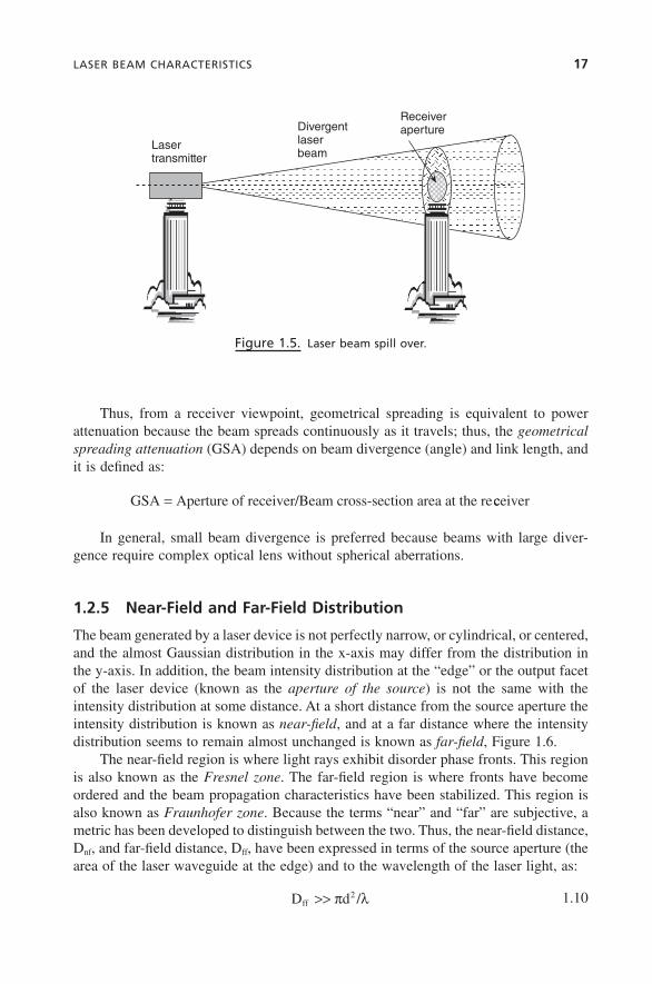
Geometrically, beam divergence or spreading is the derivative of the beam radius with respect to the distance from the beam waist. Beam divergence has an important effect at the receiver: the optical power per square unit area of the beam cross - section weakens fast as it propagates, and because the receiving photodetector has a small detecting area, a fraction of a square centimeter or few square millimeters, the optical power that impinges onto the photodetector is very small and the remaining power of the laser beam spills over, Figure 1.5 .


Thus, from a receiver viewpoint, geometrical spreading is equivalent to power attenuation because the beam spreads continuously as it travels; thus, the geometrical spreading attenuation (GSA) depends on beam divergence (angle) and link length, and it is defi ned as:

GSA Aperture of receiver/Beam cross-section area at the re= cceiver

In general, small beam divergence is preferred because beams with large diver-gence require complex optical lens without spherical aberrations.

1.2.5 Near - Field and Far - Field Distribution

The beam generated by a laser device is not perfectly narrow, or cylindrical, or centered, and the almost Gaussian distribution in the x - axis may differ from the distribution in the y - axis. In addition, the beam intensity distribution at the “ edge ” or the output facet of the laser device (known as the aperture of the source ) is not the same with the intensity distribution at some distance. At a short distance from the source aperture the intensity distribution is known as near - fi eld , and at a far distance where the intensity distribution seems to remain almost unchanged is known as far - fi eld , Figure 1.6 .

The near - fi eld region is where light rays exhibit disorder phase fronts. This region is also known as the Fresnel zone . The far - fi eld region is where fronts have become ordered and the beam propagation characteristics have been stabilized. This region is also known as Fraunhofer zone . Because the terms “ near ” and “ far ” are subjective, a metric has been developed to distinguish between the two. Thus, the near - fi eld distance, D nf , and far - fi eld distance, D ff , have been expressed in terms of the source aperture (the area of the laser waveguide at the edge) and to the wavelength of the laser light, as:

D d /ff >> π λ2 1.10

Figure 1.5. Laser beam spill over.

Lasertransmitter

Divergentlaserbeam

Receiveraperture


and

D d /nf << π λ2 1.11

Which of the two parameters (D ff or D nf ) is more suitable depends on optical design requirements. For monochromatic light, and if focusing lens are incorporated in the design, then the far - fi eld is better suited. In addition, the far - fi eld angular dispersion is superior to the near - fi eld. If on the other hand, the laser light needs to be coupled in another waveguide in the vicinity of the laser, the near - fi eld may be better suited. For laser diodes with divergent beams, the near - fi eld is few microns from the output facet. If the far - fi eld divergence angle is θ , and the near - fi eld width is w, a beam parameter for a given wavelength λ , K, is defi ned as:

K / w= 4λ π θ 1.12

Occasionally, a similar parameter M is used, defi ned as M /K= 1 . Typically, laser manufacturers provide near - and far - fi eld data for their devices.

1.2.6 Peak Wavelength

Laser devices do not source a purely monochromatic beam. In practice, they source a continuum of wavelengths in a narrow spectral range with a near - Gaussian distribution. The wavelength with the highest radiant intensity of the source is known as peak wave-length . The wavelength spread at either side of the peak is measured in nm; e.g., 1550 + / − 2 nm indicates that 1550 is the peak wavelength with a Gaussian spread at either side of 2 nm.

A monochromator is a narrow band - pass fi ltering device that allows a very narrow spectral band to pass through it.

1.2.7 Degree of Coherence

Laser beams, by defi nition may be considered coherent; that is, the wavefront of all rays departing the laser device are in phase. However, this is not absolutely true. For

Figure 1.6. Defi nition of near fi eld and far - fi eld of laser beams.

Near-Field Dnf << πd2/λ

Far-Field Dff >> πd2/λ Plane

Laser

x-axis

y-axis

Device aperture, d


example, in simple interference experiments, when the intensity minima and maxima of the fringes in the interference pattern are well defi ned and crisp, the beam is coher-ent , and when they are not (the pattern appears blurry), the beam is incoherent .

The degree of coherence (DoC) corresponds to the percent of rays in phase in the beam. For example, if in an interference experiment the minimum and maximum inten-sity of the fringed pattern is I min and I max , respectively, then the degree of coherence is defi ned as:

DoC I I / I I= − +( ) ( )max min max min 1.13

In general, a beam is considered coherent when the degree of coherence is above 0.88, partially coherent if it is less than 0.88 but above 0.55, and incoherent if it is < 0.5.

Notice that, although a sourced beam may start being coherent, as the beam travels through matter with non - uniform dielectric, DoC may change. Thus, the length of travel during which the beam remains coherent ( > 0.88) is known as the coherence length , and correspondingly, the travel time along this length is known as the coherence time .

When coherency of two interacting rays varies with time, then a time varying interferogram is produced known as a speckle pattern . In FSO systems, this in fact gives rise to the phenomenon of scintillation [12] .

1.2.8 Photometric Terms

For comparison between two light sources or two illuminated objects, the following measurable units are introduced.

• (Total) luminous fl ux , Φ , is the rate of optical energy fl ow (or number of photons per second) emitted by a point light source in all directions; it is measured in lumens (lm). In radiometric terms this is known as optical power and it is mea-sured in Watts.

• Luminous (or candle ) intensity , I, is the rate emitted in a solid angle of a spherical surface area equal to its radius (e.g. radius = 1 m, surface area = 1 m 2 ). Luminous intensity is measured in candelas or candles (cd). The luminous intensity of a sphere is Φ /4 π .

• Illuminance , E, is the fl ux density at an area A (m 2 ), or the luminous fl ux per unit area; it is measured in lux (lx). The illuminance at a point of a spherical surface is E = Φ /4 π R 2 . Illuminance refers to light received by a surface. Since the luminous intensity I of the sphere is Φ /4 π , then E = I/R 2 . This is known as the law of inverse squares , Figure 1.7 .

• Luminance , B, is the amount of optical energy emitted by a lighted surface per unit of time and per unit of solid angle and per unit of projected area is known as. Luminance is measured in cd/m 2 and is also known as nit (nt).


Table 1.1 summarizes the photometric units that are used in optics and optical communications, their measuring units and their dimensions (M = mass. T = time, L = length):

1.2.9 Radiometric Terms

Similarly, there are radiometric terms defi ned as follows:

• Radiant power ( φ ) or optical power is the rate of fl ow of radiant energy and it is measured in Watts (W).

• Radiant energy (Q) is the energy transferred by electromagnetic waves. It is the time integral of radiant power and it is measured in joules (J).

• Radiant intensity (I) is the radiant power per unit solid angle and it is measured in Watts/steradiant (W/sr).

• Radiance (L) in a given direction is the radiant intensity per unit of projected area of the source as viewed from that direction, and it is measured in W/sr - m 2 .

Figure 1.7. Illustration of the law of inverse squares.

Clear blue sky: 10 4

Sun: 1.6 × 10 9

Candle: 2 × 10 6

Fluorescent lamp: 10 4

Some examples of luminance are (in cd/m 2 ):


TABLE 1.1. Photometric Units (M = mass. T = time, L = length)

Defi nition Photometric unit Dimensions

Energy: Luminous energy (talbot) ML 2 T − 2 Energyper unit area: Luminous density (talbot/m 2 ) MT − 2 Energyper unit time: Luminous fl ux (lumen) ML 2 T − 3 Flux per unit area: Luminous emittance (lumen/m 2 or lambert) MT − 3 Flux per unit solid angle: Luminous intensity (lumen/steradian) ML 2 T − 3 Flux per unit solid angle per unit projected area:

Luminance (candela/m 2 ) MT − 3

Flux input per unit area: Illuminance (meter - candela) MT − 3 Ratio of refl ected to incident fl ux:

Luminous refl ectance

incident fl ux: Luminous transmittance Ratio of absorbed to incident fl ux:

Luminous absorptance

• Spectral radiance (L λ ) is the radiance per unit wavelength interval at a given wavelength, and it is measured in Watts/steradiant - unit area - wavelength interval (W/sr.m 2 .nm).

• Irradiance (E) or power density is the radiant power per unit area incident upon a surface, and it is measured in Watts/square meter (W/m 2 ).

• Spectral irradiance (E λ ) is the irradiance per unit wavelength interval at a given wavelength, and it is measured in Watts/unit area - unit wavelength interval (W/m 2 .nm).

1.2.10 Beam Power and Intensity

The optical power P(r, z) through a circular hole of radius r in the transverse plane at point z of the propagation axis is calculated from:

P z P r / w zo( , ) [ exp{ ( ( )}]r = − −1 2 2 2 1.14

where P o is the power of the beam emitted by the laser:

P I W /o o o= π 2 2. 1.15

where I o is the peak intensity of the beam. The above relationship is approximated for a circle of radius r = w(z) as

P z e P Po o( , ) ( ) . .r = − =1 0 8652 1.16

Thus, if the radius is r = 1.224 w(z), then 95% of the beam power will fl ow through the circle.


Similarly, the peak intensity I(z) at a distance z from the beam waist is twice the average intensity, which is obtained by dividing the total power emitted by the laser by the area within the radius w(z).

Example: Consider a laser beam emanating from a laser device with 260 mW power, a spot size (beam cross - section) 1.5 mm diameter, and with Gaussian distribution profi le. For a beam with a divergence angle 1.5 mrad, the light intensity or irradiance (optical power/area of beam cross - section) at 3 meters is ∼ 9.2 mW/mm 2 . If divergence is reduced by 20% (down to 1.2 mrad), the irradiance at 3 meters is ∼ 12.7 mW/mm 2 , that is an improvement of ∼ 40%. This means that, as the angle of beam divergence decreases, the light intensity increases exponentially and thus the same laser beam is useable over longer distance.

1.2.11 The Decibel Unit

Optical power, power attenuation and optical loss are measured in decibel units (dB). Power in decibel units is defi ned as ten times the logarithm (base 10) of power (in Watts):

Power dB P Watts( ) log [ ( )]= 10 10 1.17

In communications, the transmitted optical signal is at extremely low power, in the order of milliwatts. To denote this, the decibel unit is expressed in dBm:

Power dBm P mWatts PX W( ) log[ ( )] log[ ( )]= = −10 10 10 3

Here, few properties of logarithms are reminded, Table 1.2 , as they play a key role in the understanding of dos and don ’ ts when dealing with decibels.

TABLE 1.2. Properties of Logarithms

1. log(AB) = log A + logB 2. log(A/B) = logA − logB 3. log(A N ) = N logA 4. log {Nroot(A)} = (1/N)logA 5. log10 = 1 6. log1 = 0 7. logA = log(e) lnA 8. log (e) = log(2.71828 + ) = 0.434294 9. ln10 = 2.30258 +

10. ln2.71828 = 1 11. log A = + logA, where A > 1 12. log A = − log|A|, where 0 < A < 1 13. log(A + B) not equal to logA + logB


When adding/subtracting dBs and dBms, caution should be taken regarding the mix - and - match of units. Decibel units are additive if their argument is multiplicative, and therefore, if the units are not handled correctly one may make a serious erroneous calculation.

Power attenuation or power loss is also expressed in decibel units. In this case, it is (ten times) the logarithm of the ratio of received power over transmitted power, both expressed in the same units and thus the ratio is dimensionless. Hence, the attenuation over a fi ber span is expressed in dB, regardless whether the power is in W or mW units):

α λ( ) log ( )= 10 1 2P /P dB 1.18

As an example, a power ratio of 1000 is 30 dB, of 10 is 10 dB, of ∼ 3 is 5 dB, of 2 is ∼ 3 dB, and a ratio of 0.1 is − 10 dB. To the untrained eye and mind, loss or gain in dB ’ s is very abstract as we are trained to think of loss and gain in ratios, such as for example, 100 times less or 100 times more versus 20 dB. However, the dB is a more convenient unit and in optical communications it is widely used.

Besides decibels, power loss is also provided as a percent of power transmitted compared with that received, such as 60%, and so on. That is, if 100 units of power were transmitted and 60 were received, the loss is 100 – 60 = 40 and in percent it is (100 – 60)/100. The correspondence of dB to percent is easy to calculate. For example, 90% power loss corresponds to 10log{(100 – 90)/100} = − 10 dB, 50% corresponds to 10log0.5 = − 3 dB and 2% to 10log0.98 = − 0.01 dB. Table 1.3 lists conversions from dB loss to % loss and from % loss to dB loss.

A power ratio that is widely used in communications is the signal - to - noise (SNR), also expressed in dB units.

1.2.12 Laser Safety

The optical spectrum used in communications is invisible to the human eye. Although the eye has high absorbance in 1550 nm, nevertheless the general rule is that it is very

TABLE 1.3. Conversion from dB loss to % and from % to dB loss

dB loss %loss %loss dB loss

0 0 0 0 − 0.1 − 2.3 − 0.5 − 0.02 − 0.5 − 10.9 − 1 − 0.04 − 1 − 20.6 − 5 − 0.22 − 2 − 36.9 − 10 − 0.46 − 5 − 68.4 − 40 − 2.22

− 10 − 90.0 − 90 − 10.00 − 20 − 99.0 − 99 − 20.00


risky to look straight into a laser beam or into a lit fi ber; this invisible light may be at a power level or at an irradiance that can permanently damage the cornea and/or the retinal sensors . Retinal sensors do not regenerate and once they are damaged they remain so.

The eye physiology is such that an image is focused onto the retina where there are about 130 millions of light sensors, rods and cones, the axons of which send elec-trochemical signals to other retinal neurons where image preprocessing takes place, and from where other signals are sent via the optic nerve to the brain for fi nal post - processing.

Now, because the eye automatically focuses light, a beam with cross section 1 cm 2 on the lens is concentrated to less than 20 μ m 2 onto the fovea. This represents an enor-mous power density factor, such that 1 W/cm 2 on the lens becomes many kW/cm 2 on the fovea, which may damage it permanently.

There are two factors to consider in retinal damage, radiance of the beam and time of exposure (continuous or pulsed beam), and one safety rule, use laser eye protectors. A source is considered continuous if it emits light continuously from 0.25 to 30,000 seconds; below 0.25 sec, it is considered pulsed, and ordinary eye protectors made with polycarbonate can withstand irradiances up to 100 W/cm 2 (1 MW/m 2 ) at 10.6 μ m for several seconds.

Federal law mandates affi xing the classifi cation of the laser source on the device.

1.2.13 Classifi cation of Lasers

The transmitter and specifi cally the light source is one of the key components in optical communications systems. Light sources must be compact, monochromatic, stable, and have a long lifetime (many years). Stability implies constant optical power level and wavelength (over time, voltage and temperature variations), that is, no power variation and wavelength drift. In practice, because there are no absolute monochro-matic light sources, a very narrow band of wavelengths with a Gaussian distribution is desirable.

Light sources are classifi ed as coherent (when all emitted photons are in phase) and incoherent (when emitted photons have random phase).

The fi rst classifi cation includes all lasers and the second includes light emitting diodes (LED) and incandescent sources.

Light sources are also classifi ed as continuous wave (CW), and as directly modulated .

In communications, CW sources require modulators that are placed in the optical path. In this arrangement, an electrical signal representing a data stream acts upon the modulator affecting the continuous fl ow of light. Modulators are affected by the appli-cation of a modulated voltage, current, or light. They may be external or integrated with the laser device, Figure 1.8 .

Based on the maximum accessible emission limits (AEL), or the driving optical power (in Watts), or the energy (in Joules) by wavelength and exposure time, light sources had been classifi ed in four classes, from class 1 (no hazard when used in


normal ways) to class 4 (hazardous to eye and skin). Because since 1970 laser tech-nology has been advanced and laser applicability has been expanded, the classifi cation system has been revised (IEC 60825 – 1, edition 2.0, March 3, 2007, is applicable to safety of laser products emitting laser radiation in the wavelength range 180 nm to 1 mm).

Under the old system, in the United States the class numbers were the Roman numerals (I to IV), and in the European Union the Arabic numerals (1 – 4). The revised system uses numerals (1 – 4) in all jurisdictions. The revised four classes and their sub-classes are:

Figure 1.8. A light modulator can be external (A) or integrated with the laser device (B);

CW = continuous source.

V+

V+

V–

V∼

V∼

CWsource

CW sourcesection

Modulator

Modulationsection

Modulatedlight

Isolationbarrier

Modulatedlight

A

B


• Class 1 : This class includes high - power lasers within an enclosure that prevents exposure to the radiation; the enclosure cannot be opened without shutting down the laser. A class 1 laser is safe under all conditions in normal use; that is, the maximum permissible exposure (MPE) is not exceeded. For example, a continuous laser at 600 nm (visible) can emit up to 0.39 mW, but for shorter wavelengths the maximum emission is lower because potentially those wave-lengths can generate photochemical damage. The maximum emission is also related to the pulse duration, in the case of pulsed lasers, and to the degree of spatial coherence.

• Class 1M : Class 1M lasers produce large - diameter beams, or beams that are divergent. A Class 1M laser is safe for all conditions of use except when passed through magnifying optics such as microscopes and telescopes. If the beam is refocused, the hazard of Class 1M lasers may be increased and the product may be reclassifi ed. A laser can be classifi ed as Class 1M if the total output power is below class 3B but the power that can pass through the pupil of the eye is within Class 1.

• Class 2 : Class 2 applies to visible - light lasers (400 – 700 nm). Class - 2 lasers are limited to 1 mW continuous wave, or more if the emission time is less than 0.25 seconds, or if the generated light is not spatially coherent. Because the blink refl ex of the eye limits the laser exposure to no more than 0.25 seconds, Class 2 laser is safe, unless the the blink refl ex is intentionally suppressed. Many laser pointers are class 2.

• Class 2M : As with class 1M, this class applies to laser beams with a large diameter or large divergence, for which the amount of light passing through the pupil cannot exceed the limits for class 2. Thus, a Class 2M laser is safe because of the blink refl ex if not viewed through optical instruments.

• Class 3R : Visible spectrum continuous lasers in Class 3R are limited to 5 mW; for other wavelengths and for pulsed lasers, other limits apply. A Class 3R laser is considered safe if handled carefully, with restricted beam viewing. With a class 3R laser, the MPE can be exceeded, but with a low risk of injury.

• Class 3B : A Class 3B laser is hazardous if the eye is exposed directly, but diffuse refl ections such as from paper or other matte surfaces are not harmful. Continuous lasers in the wavelength range from 315 nm to far infrared are limited to 0.5 W. For pulsed lasers between 400 and 700 nm, the limit is 30 mJ. Other limits apply to other wavelengths and to ultrashort pulsed lasers. Protective eyewear is typi-cally required when directly viewing a Class 3B laser beam. Class 3B lasers must be equipped with a key switch and a safety interlock.

• Class 4 : Class 4 lasers include all lasers with beam power greater than Class 3B. By defi nition, a Class 4 laser can burn the skin, in addition to potentially causing permanent eye damage as a result of direct or diffuse beam viewing. These lasers may ignite combustible materials, and thus may represent a fi re risk. Class 4 lasers must be equipped with a key switch and a safety interlock. Most entertainment, industrial, scientifi c, military, and medical lasers are in this category.


Because many lasers in use were manufactured before the revised classifi cation, the old classifi cation is [found in 13 ]:

• Class I : Class I includes all lasers for which the power is low so that there is no eye damage even after hours of exposure. This includes more hazardous laser devices, which however are in enclosures preventing user access to the laser beam during operation, such as CD players. Laser sources must satisfy Class I Laser Safety requirements according to the US Food and Drug Administration (FDA/CDRH) and international IEC - 825 standards.

• Class II : Class II are low power laser sources that dot impose hazard due to the blinking of the eye. However, prolonged exposure may cause damage. Class II are lasers emitting light in the visible spectrum (0.4 to 0.7 mm) at an average power up to 1 mW power, and if applicable a pulse duration of less than 0.25 seconds. The blink refl ex of the human eye (known as aversion response ) will prevent eye damage An example of a Class II laser is a HeNe laser pointer of 1 mW or less.

• Class IIa : Class IIa are lasers emitting light in the visible wavelengths (0.4 to 0.7 mm) which produce a burn to the retina if directly and continuously viewed in excess of 1000 seconds. Supermarket laser scanners are in this subclass.

• Class IIIa : Class IIIa laser sources when viewed for < 0.25 seconds are not hazardous. However, they may be if the exposure is prolonged or if the laser beam is focused by a lens. Class IIIa are medium power lasers 1 to 5 mW and they represent a potential hazard to the eye. Beam power density may not exceed 2.5 mW/square cm. Class IIIa includes lasers with an accessible output power between 1 to 5 times the Class I AEL for wavelengths shorter than 0.4 μ m or longer than 0.7 μ m, or less than 5 times the AEL for wavelength between 0.4 and 0.7 μ m. Lasers applicable to fi rearms and laser pointers are in this category.

• Class IIIb : Class IIIb laser sources may cause damage if viewed directly or through specular refl ections but do not produce hazardous refl ections. Class IIIb lasers are typically less than 0.5 W average power. The hazard for IIIb lasers is potentially greater than that for IIIa. The hazard is still limited to direct viewing of the laser beam. These lasers do not produce hazardous diffuse refl ections or represent a skin exposure hazard. Protective eyewear is recommended when direct beam viewing. Lasers at the high power end of Class IIIb may also present a fi re hazard and can lightly burn skin.

• Class IV : Class IV laser sources cause damage if viewed directly or through specular refl ections and produce hazardous refl ections. Class IV lasers are at 0.5 W and higher. These lasers represent hazards (eye damage, skin injury, and or potential fl ammable material ignition source) for direct viewing, viewing of diffuse refl ections, and skin exposure. Most entertainment, industrial, scientifi c, military, and medical lasers are in this category.


Note: Multiwave lasers are classifi ed (with the old or the revised system) according to the most hazardous wavelength or the most hazardous possible wavelength confi guration.

In general, laser sources in communications are of class 1 or class I with Hazard Level 3A. System designers and fi ber connector designers take precautions so that there is automatic power laser shutdown (APSD) as soon as a fi ber is disconnected from the source and particularly where laser power radiation exposure is greater than 50 mW (17 dBm). Standards that describe recommendations for laser safety are:

• The ITU - T recommendation G.664 provides optical safety procedures.

• The American National Standard Institute (ANSI Z136.1 - 2000) provides maximum permissible exposure (MPE) limits and exposure durations, from 100 fempto - seconds to 8 hours.

• Similarly, the American Conference of Governmental Industrial Hygienists (ACGIH) provides the threshold limit values (TLV) and biological exposure indices (BEI).

• Both ANSI and ACGIH have become the basis for the U.S. Federal Product Performance Standard (21 CFR 1040).

In summary, depending on intensity of the source, laser sources in the range 700 – 1400 nm may cause retinal burn and promote cataract, whereas lasers in the range 1400 – 3000 nm may cause corneal burn, may affect the protein of the aqueous humour of the eye, and may promote cataract; the optical communications spectrum is in the range 1280 – 1620 nm, whereas the most used wavelengths in FSO are in the range 700 – 800 nm and in the range around 1550 nm.

1.3 ATMOSPHERIC LAYERS

The atmosphere is retained by the Earth ’ s gravitational fi eld and it consists of a mixture of gases that form a layer surrounding Earth [14] . The overall atmosphere consists approximately of (by volume) 78.00% Nitrogen, 21% Oxygen, 1% Argon, 0.04% Carbon dioxide, and other gases in smaller amounts (He, Ne, CH 4 , H 2 , Kr, and others), ∼ 1% vapor, natural and manmade aerosols and pollutants (fl uorine, chlorine, mercury, sulfur dioxide (SO 2 ), as well as dust, spores, pollen, and other; notice that this composi-tion fl uctuates within a year; the mass of atmosphere (or the total mean mass) is 5.1480 × 10 18 kilograms (kg) with an annual range due to water vapor of about 1.5 × 10 15 kg.

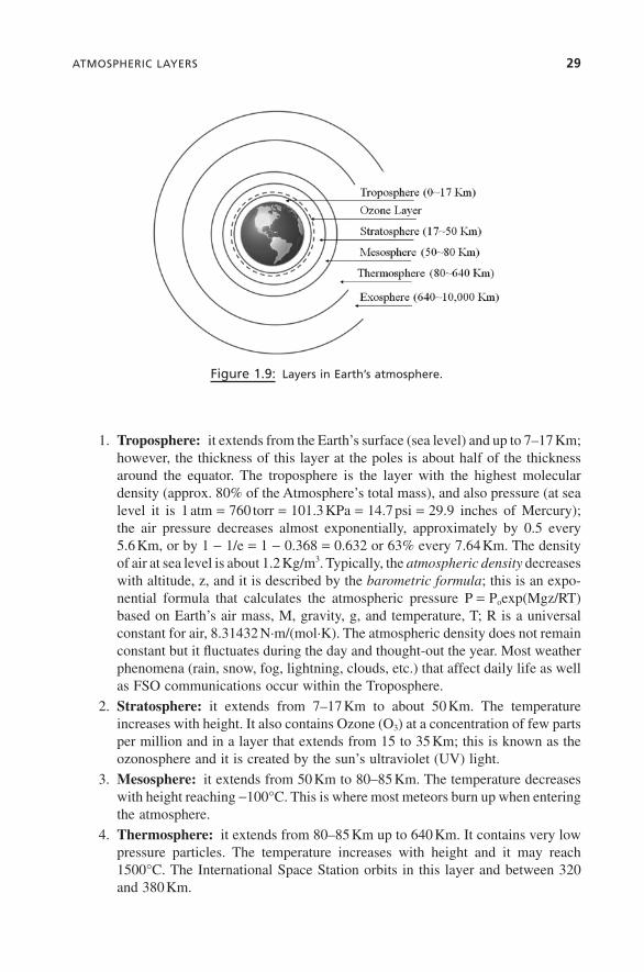
Because of the gravitational fi eld, the vertical distribution of gases is not uniform, the density of gases is not equally distributed vertically from the surface of the earth, and the pressure is not the same at all heights. In addition, the temperature of the atmosphere varies with altitude. As a result, three quarters of the atmosphere ’ s mass is within 11 Km from the surface. Because at different heights from the surface of the Earth there are different effects, the atmosphere is distinguished in layers (from lowest to highest), Figure 1.9 :

ATMOSPHERIC LAYERS 29

1. Troposphere : it extends from the Earth ’ s surface (sea level) and up to 7 – 17 Km; however, the thickness of this layer at the poles is about half of the thickness around the equator. The troposphere is the layer with the highest molecular density (approx. 80% of the Atmosphere ’ s total mass), and also pressure (at sea level it is 1 atm = 760 torr = 101.3 KPa = 14.7 psi = 29.9 inches of Mercury); the air pressure decreases almost exponentially, approximately by 0.5 every 5.6 Km, or by 1 − 1/e = 1 − 0.368 = 0.632 or 63% every 7.64 Km. The density of air at sea level is about 1.2 Kg/m 3 . Typically, the atmospheric density decreases with altitude, z, and it is described by the barometric formula ; this is an expo-nential formula that calculates the atmospheric pressure P = P o exp(Mgz/RT) based on Earth ’ s air mass, M, gravity, g, and temperature, T; R is a universal constant for air, 8.31432 N · m/(mol · K). The atmospheric density does not remain constant but it fl uctuates during the day and thought - out the year. Most weather phenomena (rain, snow, fog, lightning, clouds, etc.) that affect daily life as well as FSO communications occur within the Troposphere.

2. Stratosphere : it extends from 7 – 17 Km to about 50 Km. The temperature increases with height. It also contains Ozone (O 3 ) at a concentration of few parts per million and in a layer that extends from 15 to 35 Km; this is known as the ozonosphere and it is created by the sun ’ s ultraviolet (UV) light.

3. Mesosphere : it extends from 50 Km to 80 – 85 Km. The temperature decreases with height reaching − 100 ° C. This is where most meteors burn up when entering the atmosphere.

4. Thermosphere : it extends from 80 – 85 Km up to 640 Km. It contains very low pressure particles. The temperature increases with height and it may reach 1500 ° C. The International Space Station orbits in this layer and between 320 and 380 Km.

Figure 1.9: Layers in Earth ’ s atmosphere.


5. Ionosphere : it extends from 50 – 1000 Km. It contains charged (ionized) par-ticles and therefore it is important to radio communications.

6. Exosphere : it extends from 5000 – 1000 Km up to 10,000 Km. It borders the outer space and it contains few particles, which however cause atmospheric drag on satellites.

The interface between two successive layers have also names, such as that between the troposphere and the stratosphere is called tropopause , between the stratosphere and the mesosphere is called stratopause , and the one between the mesosphere and the thermosphere is called mesopause .

Notice that the aforementioned layers (thickness and positioning) vary continu-ously within a day and their borders overlap. The actual air pressure, density, tempera-ture and molecular consistency in each depend on the relative position of moon and sun with respect to the Earth ’ s surface, on solar activity, and on many other factors.

In the following section, we focus on the Troposphere and particularly on the phenomena that affect FSO communications.

1.4 ATMOSPHERIC EFFECTS ON OPTICAL SIGNALS

FSO technology in terrestrial applications depends on the propagation of the laser beam through the troposphere. The troposphere is the layer in which many weather phenomena occurs, which interact with and affect the quality of the propagating optical signal.

Although weather predictions can be made with the help of radars and weather satellites, overall, the troposphere is a highly dynamic and unstable medium; it consists of gases, vapor, airborne dust, natural and manmade aerosols, pollutants, and other particles, which with sunlight, temperature and pressure variation continuously move and change their consistency and characteristics so that a dynamic model of the tropo-sphere is highly complex and diffi cult to construct [15, 16] .

All molecules and particles in the troposphere interact with light and, in addition to chemically interacting, they cause absorption, scattering, fog attenuation, rain attenu-ation, snow attenuation, scintillation, lightning discharges, atmospheric tides, and other effects that affect the FSO optical propagating signal.

As such, in free space optical communication, the troposphere as propagation medium should be examined and understood. The understanding of tropospheric phe-nomena and how they affect the propagating light helps to better engineer effective, intelligent and cost - effi cient FSO links and reliable networks with the ability to self - adjust laser emission power and receiver sensitivity, self - control link alignment, self - balance network traffi c load, and self - avoid affected areas in order to provide uninterrupted service at the expected quality.

In this section, we examine the most important tropospheric phenomena that affect FSO communications. However, because the refractive index of air is an important parameter that affects light propagation through it, we will start with it.

ATMOSPHERIC EFFECTS ON OPTICAL SIGNALS 31

1.4.1 Refractive Index of Air

The index of refraction of the atmosphere has been an important parameter in the study of light propagation through it; the study of the index of refraction of air is highly complex due to the many variables that continuously change under dynamic conditions, some predictably and some unpredictably. Thus, some studies started as early as 1700, predominantly motivated by astronomical observations. For example, differential refraction due to atmospheric refractive index variation, and depending on the wave-length of observation, causes the image of an object to appear at different positions in the focal plane of a telescope.

With the advent of technology and particularly the computer, last century witnessed a signifi cant impetus in modeling the index of refraction of the air. Although the purpose of this section is not to provide a complete historical overview of the developed models on the refraction index of air, it is of interest to briefl y look into some models, as they are still in use and because FSO is a benefi ciary of a large body of research in atmo-spheric refractive index modeling [17] .

In 1939, Barrell and Sear [18] formulated the fi rst mathematical model of the refractive index of air in the visible spectrum at T = 0 ° C and P = 452 mmHg.

In1953, Edl é n formulated an empirical model by fi tting a curve on data for the refractive index of “ standard air ” at a vacuum wavelength of λ vac ( μ m); that is, air at temperature T = 15 ° C (288.15 ° K), atmospheric pressure P = 760 mmHg (1013.25 mbar), and containing 300 ppm CO 2 [19] , which is:

( ) . ( ) ( )n / /− × = + − + −− −1 10 6432 8 2949810 146 25540 418 2 2λ λ 1.19

where n is the refractive index, and λ is the wavelength (in μ m) in vacuum. In 1966, this model was revised and it was corrected; after re - fi tting the data, the

number 41 in the denominator was replaced by the number 38.9 [20] . In 1967, Edl é n ’ s formula was revised by Owens [21] who consired air compress-

ibility effects deviating from the ideal gas. In 1972, Peck and Reeder [22] made new measurements in the infrared region (IR),

with a refractive index accuracy of 2 parts in 10 9 in the region 230 nm (UV) to 1.69 mm (near IR); FSO is within this region because it uses wavelengths at ∼ 800 nm and 1.55 mm.

In 1981, Jones reconsidered the real - gas and formulated his own model [23] ; sub-sequent to this, more models have been formulated [24 – 31] in an attempt to consider water and CO2 in the atmosphere, and also other parameters that affect the refractive index of air in an attempt to provide the most accurate model.

1.4.2 Atmospheric Electricity

Atmospheric electricity, between clouds and between cloud and earth ’ s surface, builds up a typical voltage differential that ranges from 20,000 Volts to 100 Mega - Volts, which can cause multiple lightning discharges through the atmosphere, each up to 35,000 Amperes.


Lightning emits fl ashes of electro - magnetic waves from very long to very short wavelength, such as radio waves (RF, VHF, UHF), optical, x - rays, and up to gamma rays. The plasma temperature in the lightning can reach 28,000 ° K and the electron density may exceed 10 24 e − /m 3 [32] . The duration of each fl ash is between 20 to 130 msec; in FSO communications at 1 Gb/s, 100 msecs fl ash is equivalent to 10 8 bits (or 12.5 Mbytes), which corresponds to substantial data loss if the fl ash interferes with the signal at the receiver.

1.4.3 Atmospheric Tide

Vapor and ozone absorb the Sun ’ s periodic radiation causing atmospheric tides in the Troposphere and in the Stratosphere. Atmospheric tides propagate in an atmosphere where density varies signifi cantly with altitude causing wind, temperature, density and pressure fl uctuations with a periodic oscillation of about 24 hours. Near ground level, atmospheric tides are manifested with semidiurnal pressure minima (at 4 am and 4 pm local time) and pressure maxima (at 10am and 10 pm local time) [33] .

1.4.4 Defi nitions

1.4.4.1 Parts Per Million by Volume ( PPMV ) PPMV of an element in the air is the number that expresses the fraction of total molecules of a gas element in the unit of volume of air or by mole of air and it refers to the concentration of a gas element in the air [34] . For example, 1 PPMV is a micro - liter (10 − 6 liter) of a specifi c gas that is mixed in a litter of air.

Another unit for the concentration of a gas element in the air is the metric unit milligram per cube - meter ( μ g/m 3 ). To convert PPMV to μ g/m 3 one needs the density of the particular gas; this is calculated using Avogadro ’ s Law that stipulates: equal volumes of gases, at the same temperature and pressure, contain the same number of molecules . Avogadro ’ s Law implies that 1 mole of gas at standard temperature and pressure (STP) has a volume of 22.71108 liters; this is also known as the molar volume of ideal gas [35] . The Internet provides PPMV to metric units converter tools, one of them found at http://www.lenntech.com/calculators/ppm/converter - parts - per - million.htm .

1.4.4.2 Visibility This is a term specifi cally defi ned for meteorology, aviation and traffi c in general. It characterizes the degree of transparency of the atmosphere in the visible spectrum; that is, as is seen by a human observer.

Visibility is measured by the runway visual range (RVR); that is, the distance a luminous parallel beam travels through the atmosphere until its intensity (or luminous fl ux) is reduced to 5% its original value.

1.4.5 Absorption and Attenuation

Atmospheric absorption is an important impairment to FSO communications. The atmosphere, and particularly the troposphere, consists of various gases and particles


that interact with, and absorb or scatter specifi c wavelengths of light that enters the atmosphere. For example, water molecules absorb wavelengths above 700 nm (IR and far IR), whereas O 2 and O 3 absorb wavelengths below 300 nm (UV light).

Atmospheric opacity (or conversely, atmospheric transmittance) studies the elec-tromagnetic radiation from the sun and from the cosmos and its selective absorption (or transmission) by the atmosphere all the way down to the ground; atmospheric opacity (or transmittance) considers the complete spectrum from radio waves to beyond gamma rays.

Most electromagnetic wavelengths are absorbed or blocked by the atmosphere; the spectrum that passes through the atmosphere and reaches the Earth ’ s surface is known as the optical window . This window spans from 300 nm to about 1100 nm, and because it includes the visible spectrum 400 – 700 nm, it is named “ optical window ” . Another window spans from about 2 cm to 11 m and thus it is named the “ radio window ” , Table 1.4 .

As the atmosphere absorbs light from the Sun and the cosmos, so it does to laser light that propagates through it. In fact, absorption is a critical impairment to FSO communications when there is dense fog or heavy snowfall. For example, although attenuation is a mere 0.2 dB/Km in a clear day, it can be 300 dB/Km in dense fog; in the latter case, the FSO link becomes inoperable.

In general, various molecules in the atmosphere selectively absorb wavelengths; the absorption coeffi cient for a given wavelength depends on the type of gas molecule, and on the concentration of molecules.

Water (fog, rain, snow) and liquid aerosols infl uence atmospheric attenuation . Aerosols (solid or liquid) have a very small size (from sub - nanometer to 100 nm) and thus they are suspended in the air. Consequently, each particle type in the air is respon-sible for light attenuation, although the actual amount of attenuation depends on mol-ecule type, size of droplet, density of particles, and on wavelength; attenuation is measured in decibels (dB/Km). In general, the longer the λ , the lower the attenuation is, and attenuation starts becoming an issue above 5 GHz.

In general, the transmissivity of light (and from it, the absorption) is expressed by the Beer ’ s law, also known as the Beer - Lambert law. Transmissivity of transparent matter is defi ned as the ratio T = I/Io, where I and Io are the intensity or power after crossing the matter and the incident power, respectively.

The Beer ’ s law states that the transmissivity of light depends logarithmically on the product of the absorption coeffi cient, α , and the travel path of light through matter, L.

Now, if the absorption coeffi cient is expressed as the product of the molar absorp-tivity ε and the concentration c, or, as the product of an absorption cross section σ and the density N of absorbers, then, the transmissivity T is usually written as:

TABLE 1.4. Spectral ranges of concern to FSO in the Atmosphere

Spectral Range Band Sky Transparency Sky Brightness

1.1 – 1.4 microns J high low at night 1.5 – 1.8 microns H high very low


T for liquidsaL Lc= =− −10 10 ε ( ) 1.20

or as

T e for gasesLN= −σ ( ). 1.21

Similarly the absorbance is expresses as:

A I/Io for liquids= − log ( ) ( )10 1.22

or as

A I/Io for gases= − ln( ) ( ). 1.23

Thus, the absorbance is linear with the density of absorbers, as:

A Lc for liquids= ε ( ) 1.24

or

A LN for gases= σ ( ). 1.25

Now, because the atmosphere consists of different gases, each with different absor-bance characterists, the Beer ’ s law for the overall atmospheric absorption is:

I I m a g w r= − + + + + +0 2 3exp( ( )),τ τ τ τ τ τNO O 1.26

where τ a is the optical depth to aerosols that absorb and scatter light, τ g is the optical depth to uniformly mixed gases (mainly carbon dioxide CO 2 and molecular oxygen O 2 that absorb light, τ NO2 is the optical depth to nitrogen dioxide due to atmospheric pol-lutants, τ O3 is the optical depth to ozone that absorbs light, and τ r is the optical depth due to Rayleigh scattering; m is the optical mass factor (also called airmass factor ), which is approximated to 1/cos θ , where θ is the angle between the perpendicular to the Earth ’ s surface and the observed object (the zenith angle).

Realistically, atmospheric attenuation is extremely diffi cult to mathematically describe, although prediction models have been devised as well as experimental or empirical models that in general are applicable to specifi c locations and to specifi c applications [36 – 38] . Among these models, the Longley - Rice model [39 – 42] predicts transmission loss for tropospheric communication and maps data over irregular terrain and it has been adopted as a standard by FCC. However, this standard pertains to signals from 20 MHz to 40 GHz and for path lengths from 1 Km to 2000 Km; thus, the optical regime is a topic that is currently under study and a reliable and effi cient model is still in need. Another one is the Kruse model [43 ] , which provides a semi - empirical formula that relates meteorological visibility to optical atmospheric attenuation, from the visible


to near IR for dust and aerosol and for fog, if fog particles are much smaller than the wavelength:

Γ( , ) ( ) ( ) . ( )V /V / xV dB/km/λ λ= × ×17 550 0 581 1 3 1.27

where V is the visible range in Km, and λ the wavelength of the laser light. The latter formula is also simplifi ed to:

Γ( , ) ( )V k/V dB/kmλ = 1.28

where k is a unit - less coeffi cient in the range 8.5 – 17 dB that depends on wavelength; Kruse predicts k = 12 at 1550 nm. If fog particles are larger than the wavelength, then the simplifi ed Kruse formula should not be used [44] .

Atmospheric emission is the opposite of absorption. When light enters the atmo-sphere, atoms and molecules are excited and gain energy. Excited atoms then, either spontaneously or because they were stimulated emit energy, photonic or phononic (thermal). For example, the atmosphere emits infrared radiation, which may be con-tained or not if there are clouds and certain gases (CO 2 , H 2 O) or not; when it is con-tained, it gives rise to the greenhouse effect . In addition, celestial bodies emit energy. For example, the sun at approximately 6000 ° K radiates electromagnetic waves at a wavelength peak of 500 nm (visible), whereas the earth at 290 ° K radiates at a peak of 10,000 nm (invisible).

1.4.6 Fog

Fog is a cloud in contact with the ground, it is distinguished from mist only by its droplet density, and it is expressed in degree of visibility in kilometers or in meters: fog has a higher density of droplets than mist. It reduces visibility to less than 1 Km (occasionally, to less than 50 meters), whereas mist or haze reduces visibility to no less than 2 Km. As a consequence, fog attenuates light passing through it more than mist or haze. However, the attenuation coeffi cient (attenuation in dB/Km) is not the same for all electromagnetic waves but it is a function of wavelength [45 – 47] . Therefore, in communications lower frequencies that are attenuated less by fog, are advantageous. However, such frequencies are the radio frequencies that cannot support the high band-width and long link length that “ optical ” frequencies support, which are attenuated by fog much more.

Fog begins forming when water vapor at high concentration (near 100% humidity) condenses into tiny water droplets (1 – 20 μ m) in the air and when the difference between temperature and dew point is generally less than 2.5 ° C and in the presence of hydro-scopic particles in the air (that stimulate vapor condensation). Water vapor is formed by the evaporation of liquid water or by the sublimation of ice (ice to vapor). The thickness of fog is largely determined by the altitude of the inversion boundary. There are a number of mechanisms that form fog, s ome of which are briefl y described (alphabetically):


• Advection fog is formed when warm and moist air moves over a cool surface, such as land or ice, or even cooler waters. In such cases, the lower layers of the moist air are cooled down rapidly to form advection fog; this typically occurs during spring or fall.

• Artifi cial fog is fog generated by a water vaporizing machine and when the ambient temperature is cold. Power plants that emit large quantities of steam may also be included in this category.

• Diamond dust is precipitation of fi ne and sparse ice crystals falling from the clear sky.

• Flash fog is fog formed suddenly and is dissipated rapidly, as a result of tem-perature changing over the dew point.

• Freezing fog occurs when liquid fog droplets freeze to form feathery ice crystals that are deposited on the windward side of vertical surfaces, including areal wires, pylons, masts, antennas, posts, airplane wings, etc. This is common on mountain tops that are exposed to low clouds.

• Garua fog is a misty and transparent fog that occurs by the coast of Chile and Peru. When normal fog by the sea travels inland, it encounters hot air that causes the fog particles to shrink by evaporation and become almost invisible.

• Ground fog or radiation fog is formed when land cools after sunset by thermal radiation, in calm conditions and clear sky, when the ground quickly loses heat by radiation and cools the moist air above it to saturation point. Ground or radiation fog is localized, is dense and it occurs often in the fall and early winter.

• Hail fog occurs near the ground and in the vicinity of signifi cant hail accumula-tion due to decreased temperature and increased moisture. This fog is localized but it can be extremely dense and abrupt.

• Hill fog or upslope fog is formed when mild moist air ascends the slope of a hill or mountain. As the air moves up the windward side of the mountain it cools down producing fog.

• Ice fog, aka pogonip , is a type of fog that consists of fi ne ice crystals or frozen droplets that are suspended in the air. It occurs in urban areas of Polar Regions where temperature is at or below − 35 ° C. Ice fog can be extremely dense and may persist day and night until the temperature rises.

• Precipitation fog , or frontal fog , forms when fi ne rain falls into drier air below the cloud and the droplets shrink into vapor. The water vapor cools and at the dew point it condenses to form fog.

• Steam fog or evaporation fog is localized and is created by cold air passing over much warmer water or moist land.

• Valley fog forms in mountain valleys as a result of temperature inversion. It can last for several days in calm conditions. Valley fog is also known as Tule fog.

Because of the many parameters involved in fog characterization, empirical models have been developed [48] to characterize attenuation in terms of visibility based on


data taken over a period for the location of interest [49] ; as an example, the data in Table 1.5 are from [49] .

1.4.7 Smog

Smog is a combined word of smoke and fog; it actually consists of air pollution. Smog is generated by factories that emit large amounts of smoke and sulfur dioxide as a result of coal burning; now, as a result of the clean air act, this type of smog has been greatly reduced in advanced countries. However, vehicular and industrial emis-sions interact with moisture and other molecules in the atmosphere when sunlight passes through to form secondary chemical pollutants known as partriculate matter; this process is known as photochemical smog . Such polutants may be aldehydes, nitrogen oxides, peroxvacyl nitrates, and other volatile organic compounds, which are reactive and oxidizing. Photochemical smog absorbs and/or scatters the laser light used in FSO communications.

1.4.8 Rain

Rain consists of water droplets in the range of 100 μ m to 10 mm. As such, rain affects communications in the GHz range; for example, rain attenuation at 4 GHz is orders of magnitude less than attenuation at 12 GHz, a frequency typically used in satellite links. Rain also affects optical frequencies but not as much as snow does.

Rain attenuation of communications signals depends on droplet size, droplet density, rainfall rate, and the range of rain (or the rain cell) that the signal travels through [50] . Similarly, rain fade refers to absorption of RF signals. Notice that a signal may be infl uenced by rain, even though rain does not exist at the location of the transmitter or the receiver but someplace between the two.

The rainfall rate unit is mm/hr and it is measured with rain gauges over intervals of 5 minutes.

Hail is frozen rain droplets which, like rain, also affect the integrity of communica-tion signals. However, hail has a size of 5 to 50 mm.

Like snow, rain attenuation empirical models have been developed to predict optical signal attenuation from visibility range [51 – 54] ,

TABLE 1.5. Fog characterization based on empirical data (from [49] ).

Type of Fog Visibility

(m) Attenuation

(dB/Km)

Dense fog 40 – 70 250 – 143 Thick fog 70 – 250 143 – 40 Moderate fog 250 – 500 40 – 20 Light fog 500 – 1000 20 – 9.3


a /VRain = 2 9. 1.29

1.4.9 Snow

Snow, like fog and rain, has a detrimental effect in the quality of transmitted FSO optical signals.

Snow is a form of precipitation of water in the form of hexagonal ice micro - crystals due to the molecular structure of water. As these micro - crystals are created, they form fl akes and come down in one of the following forms:

• Snowfl ake is a collection of snow crystals, loosely bound together into a lace structure or a puff - ball. Snowfl akes can grow from 1 mm to about 10 cm across, and may be wet and sticky. A typical snowfl ake consists of up to 100 snow crystals.

• Snow crystals are single ice crystals with symmetrical shapes that grow directly from condensing water vapor in the air, usually around a nucleus of dust or some other foreign material. Snow crystals grow from microscopic up to a few mil-limeters in diameter.

• Rime is super cooled tiny water droplets (typically in a fog) that freeze quickly onto any surface, including snow crystals.

The snow attenuation exerted on optical signals, based on visibility range, is approximated by the empirical model [55] :

a /Vsnow = 58 1.30

1.4.10 Solar Interference

The Sun ’ s photosphere emits high intensity electromagnetic waves that are capable of interfering with electromagnetic transmission, including optical frequencies. However, solar interference occurs if the communications channel operates at the solar radiation spectrum. The solar spectrum starts from about 0.2 μ m and extends beyond 2 mm, with the highest intensity in the visible range centered about 500 nm (the visible spectrum is from 400 to 700 nm) and at an average temperature that may reach ∼ 6000 ° K; the Sun ’ s radiation also includes wavelengths in the radio, Ultra Violet (UV), X - ray and Gamma - ray bands.

Optical communications transmission is typically in the range 1280 to 1620 nm. In FSO communication systems, the most popular wavelengths are about 800 nm and about 1550 nm. Thus, there is potential solar interference, although interference is more likely to be at 800 nm than 1550 nm. However, for solar interference to be troublesome, sunlight must fall onto the photodetector. Additionally, when 1550 nm is used, a long - pass optical fi lter at the receiver may reject wavelengths below the 1300 nm to greatly reduce the solar background radiation (SBR) interference. In FSO, the Solar Background Radiation (SBR) is greatly reduced with proper housing design and with optical fi lters.


1.4.11 Scattering

As light passes through the atmosphere, photons interact with molecules and other particles and are scattered in every possible direction like billiard balls; that is, photons are defl ected by the molecules without altering their wavelength or energy. However, all photons do not interact the same way, because the actual scattering mechanism depends on the size and type of molecules and on the wavelength of light [56 – 60] .

Assuming that the airborne particles in the atmosphere are small spheres with radius r, they have a refractive index n, and that light has a wavelength λ , the size parameter σ is defi ned by:

σπλ

= − +4 2

31 2

5 6

42 2 2( )

{( ) )}r

n /n 1.31

Then, the intensity of scattered unpolarized photons at an angle θ , at a distance from the particle D, wavelength λ , and initial intensity I 0 is:

I ID

o= +3

161

22σ

πθ( cos ) 1.32

For example, nitrogen has σ = 5.1 × 10 − 31 m 2 at a wavelength 532 nm, which cor-responds to green light.

The above intensity equation may be modifi ed if scattering is by molecules, which have no well - defi ned refractive index but they have polarizability, α .

Polarizability is defi ned as the ratio of the induced dipole moment P of an atom to the electric fi eld E that produces the moment, α = P/E; that is, polarizability is the amount of charge re - distribution of a cloud of electrons in the presence of an external electric fi eld (of a nearby charged molecule or ion). In this case, for N scatterers, the intensity is:

I IN

Do= +

81

4 2

4 22π α

λθ( cos ) 1.33

Based on the particle size and the wavelength of light, three scattering mechanisms are identifi ed:

• Rayleigh Scattering when r << λ ; then σ ∼ λ − 4

• Mie Scattering when r ∼ λ ; then σ ∼ λ − 1.6 to 0

• Geometric Scattering when r >> λ ; then σ ∼ λ ≥ 0

Clearly, in the atmosphere where many different kinds and sizes of particles and molecules are present, scattering may occur by one or more of the above mechanisms. For example, a photon may be scattered by a very small particle (Rayleigh scattering), the scattered particle may then be scattered by a particle of the same order of magnitude


(Mie scattering) and then perhaps by a very large particle (Geometric scattering), and so on.

1.4.11.1 Rayleigh Scattering This occurs when the particles in the atmo-sphere are much smaller than the wavelength of light passing through them. As a consequence, Rayleigh scattering at 400 nm is approximately 10 times greater than 700 nm for equal light intensity.

In addition, the intensity of the scattered light varies as the sixth power of the particle size and varies inversely with the fourth power of the wavelength. Because of the relatively smaller size of particles compared with the wavelength and because photons have small energy (large wavelength) and no charge, Rayleigh scattering may be studied using elastic scattering equations; that is, the energy of scattered photon before scattering and after scattering are maintained but not the direction of movement. If the photon has enough energy to excite a particle (that is, to interact with some of its vibration modes), then some energy exchange may take place; this is known as Raman scattering .

As a consequence of Rayleigh scattering, shorter wavelengths (blue) scatter more than longer wavelengths (red); as a result, during the day the sky is blue from all direc-tions because what we see is the scattered light by the atmosphere ’ s molecules and particles. When viewing the sun however, what we see is unscattered light (with blue being removed by scattering) and therefore the sun looks red - yellowish. At sunset, because the sun is at the horizon or beyond it, rays travel the longest path in the atmo-sphere, the blue light has already been scattered out and only the reddish rays are the ones to reach our eyes. When viewing the Earth from the outer space, the atmosphere looks blue because what one sees is scattered light, the sky looks black and the sun white. The water droplets in clouds are much larger than the wavelength of visible light, they are the result of Mie scattering, and they look white against a blue sky.

Rayleigh scattering produces forward and backward transmission patterns like antenna lobes, which are narrower and more intense for smaller particles [61] .

Rayleigh scattering also occurs when light propagates in gases, liquids, as well as in transparent solid materials, such as optical fi ber.

In silica fi ber, the molecule density fl uctuates randomly giving rise to optical power loss due to scattering. The loss coeffi cient due to scattering, α scat , in this case is:

απλ

βscat n p T=8

3

3

48 2( )( )k 1.34

where p is the photoelastic coeffi cient of silica, k is the Boltzman constant, n is the refractive index of silica, λ is the wavelength of scattered light, and β is the isothermal compressibility.

1.4.11.2 Mie Scattering Mie scattering — the outcome of the theory of elec-tromagnetic plane wave scattering by a dielectric sphere — occurs when the radius of the particles in the atmosphere, including aerosols are about the same size as the wave-


length of light passing through it [62] . Dust, pollen, smoke, and water vapor are responsible for Mie scattering. As a consequence, Mie scattering occurs in the lower layer of the troposphere where such particles are in higher concentration, particularly during overcast conditions.

Mie scattering does not strongly depend on wavelength and it produces the whitish glare around the sun when the density of particulate material is in the atmosphere, as well as the white light from mist and fog. Mie scattering also produces a transmission forward pattern like an antenna lobe, which is narrower and more intense for larger particles, Figure 1.10 .

1.4.11.3 Geometric Scattering This occurs when particles in the atmo-sphere are many orders of magnitude larger than the wavelength; in FSO applications where laser light is 1.5 μ m, the particle size is in the order of mm. Such particles may be soil, sand and dust that become airborne during storms and strong winds in specifi c parts of the world (deserts, agricultural areas, volcanic activity, etc). In this case, scat-tering and light attenuation depends on the density of particles per cubic cm or meter, and it is much more pronounced than Rayleigh or Mie scattering. As a point of

Figure 1.10. Rayleigh scattering is bidirectional (A), whereas Mie scattering is mostly unidi-

rectional (B).


reference, Table 1.6 lists approximate radii of various molecules and particles in the atmosphere.

1.4.12 Scintillation

The atmosphere is a mixture of gases, molecules and particles that continuously gain or lose energy (heat). Some localized cells are heated more than others, whereas some others are cooled more than others. Thus, there is expansion and contraction of air cells, upward and downward movement, as well as lateral shifts. The end result is a thermal turbulence in air cells characterized by inhomogeneous and dynamically changing refractive index, density and air consistency.

When a light beam propagates through atmospheric turbulence, most of its pro-perties are affected. That is, its polarization, refraction, absorption, scattering and attenuation fl uctuate randomly at a frequency between 0.01 Hz and 200 Hz; under the same conditions, the intensity and frequency of fl uctuations increase with wave frequency.

In FSO, when the laser beam crosses atmospheric turbulence, its polarization and coherency fl uctuates due to anisotropic fl uctuations of the air mass along the path, and its attenuation constant fl uctuates due to non - consistent power loss throughout the air mass along the path [63, 64] . As a result, when the signal arrives at the receiver, its intensity fl uctuates due to random temporal and spatial irradiance fl uctuations of the beam, and the signal focuses and defocuses onto the photodetector randomly; this effect is similar to the fl ickering lights of a city in a summer night when they are viewed from far away. This signal fl uctuation due to thermal turbulence is known as scintillation .

Scintillation affects the quality of the propagating signal and the magnitude of the scintillation effect is defi ned as the ratio between its instantaneous amplitude and its average value in the unit of time, expressed in decibel units. Several theoretical models have been developed in an attempt to predict the scintillation effect [65, 66] . However, scintillation is a complex phenomenon that also depends on time - variant meteorological

TABLE 1.6. Approximate radii of various molecules and particles in the atmosphere.

Particle type Radius ( μ m)

Air molecules Approx. 0.0001 N2 0.000075 CO2 0.000323 O2 0.000292 Haze 0.01 – 1 Fog 1 – 20 Rain 100 – 10,000 Snow 1000 – 5000 Hail 5000 – 50,000


phenomena, which are diffi cult to model. Therefore, theoretical scintillation models are valuable as long as the parameters and boundary conditions they were developed for hold, and they also require validation by experimental data.

Scintillations is measured by the scintillation index, σ index , which is expressed as:

σ index I I / I2 2 2 2= < > − < > < >( ) 1.35

where I is the irradiance (or intensity) of the optical wave, and the brackets < > denote the average value over time.

In FSO communication links as well as in laser radar links, knowledge of the scintillation index is important for determining system performance. The scintillation index increases with path length, while the optical signal becomes less coherent and the focusing effect at the optical power receiver deteriorates.

To ameliorate the scintillation effect, the diameter of the collecting lens at the receiver is increased to beyond the irradiance correlation width , ρ c , of the received optical signal; the irradiance correlation width is determined from the irradiance covari-ance function, which is a Gaussian function of time, and it identifi es the maximum receiver aperture size that acts like a point receiver .

Apertures larger than ρ c perform aperture averaging , and as such, the correlation width ρ c is a design parameter that helps to reduce the amount of scintillation effect as is experienced by the photodetector of the receiver. An interesting method that uses a rotation pipe to reduce the amount of speckle has been reported [67] .

1.4.13 Wind and Beam Wander

Wind is movement of air masses that takes place in the troposphere and in the strato-sphere [68] Light itself is not affected by wind only, but perhaps what causes wind (temperature variation and other factors). However, in FSO applications, wind has a degrading effect on beam alignment because FSO transceivers are positioned on tall buildings or on poles. Strong wind turbulence can sway a tall building by few meters and thus displace the beam from its target receiver. As a consequence, the effect of turbulent winds on beam alignment may be signifi cant as the laser beam seems to wander at the receiver; this is known as beam wander . If in addition to wind, there are localized temperature variations on the beam path (which cause scintillation), then beam wander may also affect the scintillation index [69] ; this is known as beam wander induced scintillation (BWIS). Clearly, the effect of the latter depends on beam properties; BWIS is insignifi cant if the beam is collimated or is divergent, and is aggra-vated if the beam is focused. Currently, we have no signifi cant data to identify the effect on BWIS of a very thin, almost not divergent, laser beam with and without auto - tracking.

In short, the effect of beam wander depends on whether the beam is collimated, is divergent or is focused, on the diameter of the beam, and also whether the transceivers have an automatic tracking system to maintain alignment even if the position of one transceiver shifts by few meters with respect to the other.


1.5 CODING FOR ATMOSPHERIC OPTICAL PROPAGATION

FSO communications is based on an optical narrow beam that propagates through the atmosphere. The atmosphere, an unbounded medium, is very dynamic and its param-eters are not constant. Therefore, as already described, the various atmospheric phe-nomena of the troposphere have an adverse effect on the quality of the optical signal. Therefore, the obvious question: which modulation method of the optical signal would be more effective?

Drawing from the experience in fi ber optic communications, currently four methods seem to be the most probable: phase - shift keying (PSK), frequency shift keying (FSK), state of polarization shift keying (SoPSK), and amplitude or on - off keying (OOK).

• The PSK is effective if the phase remains unadulterated in the medium and along the transmission path. As we have discussed, the phase of the FSO beam changes due to refractive index changes and scintillation. Therefore, it is obvious that this modulation method will produce an increased bit error rate (BER).

• The FSK requires switching between two different optical frequencies and thus it requires two laser transmitters, or a laser transmitter and a wavelength con-verter device. Although this method could be very effective, it adds to the cost and to the design complexity of the transceivers.

• The SoPSK experiences the same issues with the PSK; the polarization is not maintained by the air medium due to the dynamic changes in refractive index of the air.

• The OOK modulation method is the most basic form of pulsed modulation and is used in binary direct detection receivers in fi ber - optic and in FSO communica-tions, for which the link performance versus link length, the signal to noise ratio (SNR), and the bit error rate (BER) have been thoroughly studied.

The performance (probability of error in terms of SNR) for OOK is:

P erfc S/Ne = 1 2 ( ) 1.36

where erfc is the error function complimentary. In FSO systems, the OOK method seems to be the most robust of the four afore-

mentioned since pulsed light with direct detection does not depend as much on phase and polarization variations, although it does on intensity.

In addition, because the performance of an FSO link can be deduced from the probability density function (PDF) of the irradiance signal, then, in the presence of air turbulence the unconditional BER is determined from the probability of error or the conditional probability averaged over the PDF of the random signal.

1.6 LIDAR

LIDAR is an acronym that stands for Laser Detection And Ranging . As the acronym states, it is based on a thin laser beam that is pulsed and emitted in the atmosphere; the

LIDAR 45

power of the beam may be from few milliWatts to many Watts. In addition, a photo-detector measures the beam refl ection to determine phase shift, intensity, and perhaps polarization state, Figure 1.11 . The laser beam may be refl ected vertically or horizon-tally, and it can be stationary or moving in a rotational mode or in a scan mode. As such, LIDARs have found applications in astronomy, in meteorology, in archaeology, in land surveying, in 3 - D object mapping, distance measurement, object detection, movement detection, and more [70 – 72] .

LIDARs use a short wavelength that typically ranges from the UV (below 400 nm) to IR (above 700 nm); that is, the complete visible spectrum and beyond. As such, the feature accuracy of objects obtained by LIDARs are very accurate, in the order of the wavelength. However, the laser beam is also susceptible to atmospheric impairments (absorption, attenuation, scattering, scintillation, etc.) as a result of molecular, aerosol, and atmospheric pollutant interaction. Although this may seem to be detrimental to LIDAR applications, in fact it is an advantage: because of the small wavelength, refl ec-tions take place by minute dielectric discontinuities or localized dielectric anomalies (caused by aerosols, smoke, and other pollutants) and not by large metallic objects as in the case of radio frequency RADARs; the long wavelength of RADAR is insensitive to small particles, like large sea waves over small pebbles are. Thus, the LIDAR has been used in atmospheric research, in weather prediction, and in air pollution identifi ca-tion and measuring.

Depending on the type and size of molecules that scatter the beam, LIDARs are classifi ed in:

• Rayleigh LiDAR,

• Mie LiDAR,

• Raman LiDAR, which exploits inelastic scattering; a small amount of the pho-tonic power interacts with gases and light is scattered with a longer wavelength which depends on the type of gas. This LIDAR is used for atmospheric gas

Figure 1.11. Principles of a LIDAR.


concentration, and for aerosol parameter measurement), as already described. Using THz interferometry, chemical, nuclear, or organic molecules can be detected from a distance.

• The differential absorption LIDAR uses an “ on - line ” or probe wavelength that is absorbed by the gas and another wavelength that is not absorbed. From the scattered light, the differential absorption is measured from which ozone, carbon dioxide, or water vapor measurements are made.

• The Elastic Backscatter (by aerosols and clouds) LIDAR.

• The Fluorescence LiDAR is based on the fl uoresce effect of certain elements (Na, Fe, K), and

• The Doppler LIDAR is similar to the Elastic Backscatter LIDAR but it measures the frequency shift of the backscattered light from which the wind speed is cal-culated. Traffi c speed enforcement uses this type of LIDAR.

Moreover, there are two more orthogonal classifi cation types of LIDARs, the coherent light and the incoherent type.

• The coherent type LIDAR uses coherent light and measurements are based on phase differences of the refl ected beam. Thus, the receiver must be a heterodyne photodetector receiver. This type is suitable for moving objects and for phase sensitive measurements.

• The incoherent type LIDAR uses incoherent light and measurements are based on the amplitude (intensity) of the refl ected beam. That is, the receiver uses a simple direct intensity photodetector.

When the LIDAR beam scans the surface of a 3 - D object, the beam is refl ected and a map of its surface may be obtained by measuring the time and/or the phase of the pulsed light that returns to the detector; thus the distance is measured with resolu-tion commensurate with the wavelength (nm) or the pulse repetition rate. The informa-tion obtained may be used to identify an object, to map or survey a terrain, to reproduce (copy) an object, and more. One of the simplest LIDAR applications is the label and barcode scanner at check - out points.

Regarding laser power, in atmospheric applications it is many Watts whereas in surveying and identifying objects is few milliWatts. More LIDAR applications are emerging including automatic vehicular guidance and control, and possibly automatic control of FSO link alignment and performance.

REFERENCES

1. S.V. Kartalopoulos , “ A Global Multi Satellite Network ” , U.S. patent #5,602,838 , 2/11/ 1997 .

2. K. Shaik , “ Atmosphere Propagation Effects Relevant to Optical Communications , ” TDA Progress Report, 42 – 94, pp. 180 – 200 , Jet Propulsion Laboratory, Pasadena, CA, August, 1988 .

REFERENCES 47

3. S.V. Kartalopoulos , DWDM: Networks, Devices and Technology , IEEE/Wiley , 2003 .

4. S.V. Kartalopoulos , Introduction to DWDM Technology: Data in a Rainbow , IEEE/Wiley , 2000 .

5. ITU - T Recommendation G.652 , “ Characteristics of a single - mode optical fi bre cable ” , Oct. 2000 (Table G.652.C lists the parameters of the water - free fi ber).

6. ITU - T Recommendation G.692 , “ Optical interfaces for Multi - channel Systems with Optical Amplifi ers ” , Oct. 1998 (Appendix VII provides bidirectional WDM transmission recom-mendations, Appendix VIII transmission of 16 and 32 channels), and Corrigentum 1, Jan. 2000 .

7. ITU - T Recommendation G.694.1 , “ Spectral Grids for WDM Applications: DWDM Frequency Grid ” , 5/ 2002 .

8. ITU - T Recommendation G.694.2 , “ Spectral Grids for WDM Applications: CWDM Wavelength Grid ” , 6/ 2002 Draft.

9. B.E.A. Saleh and M.C. Teich , Fundamentals of Photonics , John Wiley & Sons , New York , 1991 .

10. F. Pampaloni and J. Enderlein ( 2004 ). “ Gaussian, Hermite - Gaussian, and Laguerre - Gaussian beams: A primer ” . ArXiv:physics/0410021 . http://arxiv.org/abs/physics/0410021 .

11. A Tutorial on Gaussian Beam Optics , Newport: http://www.newport.com/servicesupport/Tutorials/default.aspx?id=122 ; Retrieved Jan 2011 .

12. L. Andrews , R.L. Philips , and C.Y. Hopen , Laser Beam Scintillation with Applications , SPIE Press , 2001 .

13. ANSI Z136.1 - 1993 , “ American National Standard for Safe Use of Lasers ” .

14. U.S. Standard Atmosphere , U.S. Government Printing Offi ce, Washington, D.C., 1976 . Also in http://ntrs.nasa.gov/archive/nasa/casi.ntrs.nasa.gov/19770009539_1977009539.pdf .

15. F.K. Lutgens and E.J. Tarbuck , The Atmosphere , Prentice Hall , 1995 .

16. ITU - R Recommendation P.530 - 11 , “ Propagation data and prediction methods required for the design of terrestrial line - of - sight systems , ” International Telecommunication Union, Geneva, 2005 .

17. B.A. Bodhaine , N.B. Wood , E.G. Dutton , and J.R. Slusser , “ On Rayleigh Optical Depth Calculations , ” Journal of Atmospheric and Oceanic Technology , vol. 16 , issue 11 , pp. 1854 – 1861 , Nov. 1999 . Good historical overview of refractive index modeling.

18. H. Barrell and J.E. Sears , “ The Refraction and Dispersion of Air for the Visible Spectrum , ” Philosophical Tranactions of the Royal Society A , vol. 238 , pp. 6 – 62 , 1939 .

19. B. Edl é n , “ Dispersion of standard air , ” Journal of the Optical Society of America , vol. 43 , pp. 339 – 344 , 1953 .

20. B. Edl é n , “ The refractive index of air , ” Metrologia , vol. 2 , pp. 71 – 80 , 1966 .

21. J.C. Owens , “ Optical refractive index of air: dependence on pressure, temperature and com-position , ” Applied Optics , vol. 6 , pp. 51 – 59 , 1967 .

22. E.R. Peck and K. Reeder , “ Dispersion of air , ” Journal of the Optical Society of America , vol. 62 , pp. 958 – 962 , 1972 .

23. J.W. Marini and C.W. Murray , Jr , Correction of laser range tracking data for atmospheric refraction at elevations above 10 degrees , NASA - TM - X - 70555, 1973 .

24. C.S. Gardner , Correction of laser tracking data for the effects of horizontal refractivity gradients , Applied Optics, vol. 16, pp. 2427 – 2432 , 1977 .

25. F.E. Jones , “ The refractivity of air , ” Journal Research NBS , vol. 86 , pp. 27 – 32 , 1981 .


26. P.E. Ciddor , “ Refractive index of air: new equations for the visible and near infrared , ” Applied Optics , vol. 35 , pp. 1566 – 1573 , 1996 .

27. P.E. Ciddor and R.J. Hill , “ Refractive index of air , ” Applied Optics , vol. 38 , pp. 1663 – 1667 , 1999 .

28. V. Mendes , Modeling the neutral - atmosphere propagation delay in radiometric space tech-niques , PhD. thesis, University of New Brunswick , 1999 .

29. H. Yan and G. Wang , “ New consideration of atmospheric refraction in laser ranging data , ” Monthly Notices of the Royal Astronomical Society , vol. 307 , pp. 605 – 610 , 1999 .

30. Y.S. Galkin , R. Tatevian , and L. Blank , Correction of the water vapour absorption line effect for EDM with infrared emitting diodes , 22nd General Assembly of the International Union of Geodesy and Geophysics (IUGG), 1999 .

31. P.E. Ciddor , “ Refractive Index of Air: 3. The Roles of CO 2 , H 2 O, and Refractivity Virials ” , Applied Optics , vol. 41 , pp. 2292 – 2298 , 2002 .

32. V.A. Rakov and M.A. Uman , Lightning Physics and Effects , Cambridge Univ. Press , 2003 .

33. T.F. Malone , Ed, Compendium of Meteorology , American Meteorological Society , Boston, Mass , 1951 .

34. N. Never , Air Pollution Control Engineering , McGraw - HILL , Singapore , 1995 .

35. E.R. Cohen and B.N. Taylor , Journal of Research National Bureau of Standards , vol. 92 , pp. 85 – 95 , 1987 . (International Union of Pure and Applied Chemistry (IUPAC))

36. ITU - R Recommendation P.618 - 7 , 2001 , “ Propagation Data and Prediction Methods Required for the Design of Earth - Space Telecommunication Systems ” .

37. H. Hemmati , Deep Space Optical Communications , John Wiley & Sons , 2006 .

38. P.W. Kruse and al., “ Elements of infrared technology: Generation, transmission and detec-tion ” , J. Wiley and sons, New York, 1962 .

39. A.G. Longley , “ Radio propagation in urban areas , ” OT Report 78 – 144, Apr. 1978 .

40. A.G. Longley , “ Local variability of transmission loss - land mobile and broadcast systems ” , OT Report, May 1976 .

41. OET BULLETIN No. 69 , Longley - Rice Methodology for Evaluating TV Coverage and Interference , February 2006 ; it provides guidance on the implementation and use of Longley - Rice methodology.

42. http://www.v - soft.com/probe/probeIIgalary.htm provides a gallery of map studies using the Longley - Rice model. Retrieved Nov 23, 2010 .

43. P.W. Kruse , L. McGlauchlin , and O.H. Vaughan , Elements of Infrared Technology: Generation, Transmission and Detection , John Wiley & Sons , New York , 1962 .

44. R.M. Pierce , J. Ramaprasad , and E. Eisenberg , “ Optical Attenuation in Fog and Clouds , ” Optical Wireless Communications IV, Proceedings of SPIE , vol. 4530 , pp. 58 – 71 , 2001 .

45. I.I. Kim , B. McArthur , and E. Korevaar , “ Comparison of laser beam propagation at 785 nm and 1550 nm in fog and haze for optical wireless communications , ” Proc. SPIE , 4214 , 26 – 37 , 2001 .

46. M. Al Naboulsi , H. Sizun , and F. de Fornel , Fog Attenuation Prediction for Optical and Infrared Waves , Journal SPIE, International Society for Optical Engineering, 2003 .

47. M. Gebbart , E. Leitgeb , M. Al Naboulsi , H. Sizun , and F. de Fornel , Measurements of light attenuation at different wavelengths in dense fog conditions for FSO applications , STSM - 7, COST270, 2004 .

REFERENCES 49

48. S.S. Muhammad , B. Flecker , E. Leitgeb , and M. Gebhart , “ Characterization of fog attenua-tion in terrestrial free space optical links , ” Journal of Optical Engineering , vol. 46 , no. 4 . Paper. 066001 , June 2007.

49. M.S. Awan , L.C. Horwath , S.S. Muhammad , E. Leitgeb , F. Nadeem , and M.S. Khan , “ Characterization of Fog and Snow Attenuations for Free - Space Optical Propagation , ” Journal of Communications , vol. 4 , no. 8 , pp. 533 – 545 , September 2009 .

50. M. Akiba , K. Wakamori , and S. Ito , “ Measurement of optical propagation characteristics for free - space optical communications during rainfall ” , IEICE Transactions on Communications E87 - B, 2053 – 2056 ( 2004 ).

51. D. Atlas , “ Shorter Contribution Optical Extinction by Rainfall , ” J. Meteorology , vol. 10 , pp. 486 – 488 , 1953 .

52. ITU - R Recommendation P.839 - 3 , “ Rain height model for prediction models ” , International Telecommunication Union, Geneva, 2001 .

53. ITU - R , “ Development towards a model for combined rain and sleet attenuation ” , ITUR Document 3M/62E, International Telecommunication Union, Geneva, 2002 .

54. ITU - R Recommendation P.837 - 4 , “ Characteristics of precipitation for propagation model-ing ” , International Telecommunication Union, Geneva, 2003 .

55. H.W. O ’ Brien , “ Visibility and Light Attenuation in Falling Snow , ” Journal of Applied Meteorology , vol. 9 , pp. 671 – 683 , 1970 .

56. H.C. van de Hulst , Light scattering by small particles , New York, Dover , 1981 .

57. M. Kerker , The scattering of light and other electromagnetic radiation , Academic Press , New York , 1969 .

58. C.F. Bohren and D.R. Huffmann , Absorption and scattering of light by small particles , John Wiley - Interscience , New York , 1983 .

59. P.W. Barber and S.S. Hill , Light scattering by particles: Computational methods , World Scientifi c , Singapore , 1990 .

60. D. Atlas , M. Kerker , and W. Hitschfeld , “ Scattering and attenuation by nonspherical atmo-spheric particles , ” Journal for Atmospheric and Terrestrial Physics , vol. 3 , pp. 108 – 119 , 1953 .

61. M. Sneep and W. Ubachs , “ Direct measurement of the Rayleigh scattering cross section in various gases , ” Journal of Quantitative Spectroscopy and Radiative Transfer , vol. 92 , p. 293 , 2005 .

62. G. Mie , “ Beitr ä ge zur Optik tr ü ber Medien, speziell kolloidaler Metall ö sungen , ” Leipzig, Ann. Phys , vol. 330 , pp. 377 – 445 , 1908 .

63. L.C. Andrews and R.L. Phillips , Laser Beam Propagation through Random Media , 2 nd ed. , SPIE SPIE Press , 2005 .

64. Encyclopedia of Optical Engineering , Volume 3 , R.G. Driggers , Editor, CRC Press , 2003 .

65. J. Sala , M. Lamarca , J. A. Lopez , F. Rey , J. Riba , G. Vazquez , X. Villares , A. M. Jalon , and P. Rodr ı guez , “ A Rain and Scintillation Ka - band Channel Simulator ” , 10th International Workshop on Signal Processing for Space Communications (SPSC 2008 ), 6 – 8 October 2008, Rhodes Island, Greece. Paper also available at: http://www.gts.tsc.uvigo.es/gpsc/sproactive/Documents/Papers/SPSC08.pdf .

66. L.C. Andrews , R.L. Phillips , and C.Y. Hopen , Laser Beam Scintillation with Applications , SPIE Press , 2001 .

67. M. Sun and Z. Lu , “ Speckle suppression with a rotating light pipe , ” Optical Engineering , vol. 49 , no. 2 , paper 024202 , February 2010.


68. J.A. Dutton , The Ceaseless Wind: An Introduction to the Theory of Atmospheric Motion , Dover Publications , New York , 1986 .

69. L.C. Andrews , et al., “ Beam wander effects on the scintillation index of a focused beam , ” SPIE , vol. 5793 , 2005 .

70. http://home.iitk.ac.in/ ∼ blohani/LiDAR_Tutorial/Airborne_AltimetricLidar_Tutorial.htm provides a quick tutorial of LIDARs and their applications. Retrieved Nov. 23, 2010 .

71. http://www - calipso.larc.nasa.gov/ provides a description of the Cloud - Aerosol Lidar and Infrared Pathfi nder Satellite Observation (CALIPSO) satellite used for measurements of clouds and atmospheric aerosols (airborne particles) that play a role in regulating Earth ’ s weather, climate, and air quality.

72. http://ramanlidar.gsfc.nasa.gov/ describes NASA ’ s Raman LIDAR for measuring water vapor, aerosols and other atmospheric species.

PROPAGATION OF LIGHT IN UNGUIDED MEDIA

Documents

Transcript of PROPAGATION OF LIGHT IN UNGUIDED MEDIA