Università degli Studi di Padova

Faculty of Physics

Propagation of electromagnetic

waves in “Fishnet” metamaterials

Doctoral Thesis

Dr. Giuseppe Parisi

Padua, 2012

Coordinator: Ch.mo Prof. Andrea Vitturi

Supervisor: Ch.mo Prof. Filippo Romanato

To my father

i

Summary

AbstractAbstractAbstractAbstract………………………………………………………………………………………................1111

AcknowledgementAcknowledgementAcknowledgementAcknowledgement ................................................................................................................................................................................................................................................................................................................................................................................................ 3333

1111 IntroductionIntroductionIntroductionIntroduction ................................................................................................................................................................................................................................................................................................................................................................................................ 4444

1.11.11.11.1 Historical overview ............................................................................................... 7

1.21.21.21.2 The recent interest in metamaterial. .................................................................. 10

1.31.31.31.3 Main research directions in metamaterials ......................................................... 11

1.3.1 Negative permittivity .................................................................................. 12

1.3.2 Negative permeability ................................................................................. 13

1.3.3 Perfect lens .................................................................................................. 16

1.3.4 Metamaterials cloaks ................................................................................... 17

1.3.5 Chiral and bi-anisotropic materials............................................................. 18

1.3.6 Tunable metamaterials ............................................................................... 18

1.3.7 Optic metamaterials. ................................................................................... 19

1.1.1.1.4444 The aim of the thesis .......................................................................................... 21

2222 Effective method approach to metamaterialsEffective method approach to metamaterialsEffective method approach to metamaterialsEffective method approach to metamaterials ........................................................................................................................................................................................ 24242424

2.12.12.12.1 The standard retrieval method ........................................................................... 27

2.22.22.22.2 S-parameters ....................................................................................................... 31

2.32.32.32.3 Retrieval method in presence of one or two substrate. ...................................... 34

2.42.42.42.4 S-parameters in presence of bi-anisotropy medium. ........................................... 36

2.52.52.52.5 Conclusion .......................................................................................................... 39

3333 Fishnet Fishnet Fishnet Fishnet metamaterialmetamaterialmetamaterialmetamaterial……………………………………….... ........................................................................................................ 42424242

3.13.13.13.1 Single negative µ metamaterial ......................................................................... 43

3.23.23.23.2 A DNNIM in the optical spectral range: the Fishnet metamaterial. ................. 45

3.33.33.33.3 The effective Fishnet parameters ....................................................................... 47

3.43.43.43.4 The Fishnet modes (an overview) ...................................................................... 49

3.53.53.53.5 Electric and magnetic response of metamaterial Fishnet ................................... 53

3.63.63.63.6 Parametric analysis of Fishnet metamaterial ..................................................... 56

3.73.73.73.7 Parametric simulations under D, W, h variation .............................................. 58

3.83.83.83.8 Scaling law under P and az variation .................................................................. 62

3.93.93.93.9 Scaling with dielectric permittivity dε .............................................................. 64

3.103.103.103.10 Conclusion ....................................................................................................... 65

4444 Multilayered Fishnet and bianisotropyMultilayered Fishnet and bianisotropyMultilayered Fishnet and bianisotropyMultilayered Fishnet and bianisotropy ............................................................................................................................................................................................................................ 66666666

ii

4.14.14.14.1 Negative Refractive index of a multilayered Fishnet structure. ......................... 67

4.24.24.24.2 The role of surface polaritons in multilayered Fishnet metamaterial ............... 75

4.34.34.34.3 Conclusion .......................................................................................................... 84

5555 Experimental FishnetExperimental FishnetExperimental FishnetExperimental Fishnet ................................................................................................................................................................................................................................................................................................................................ 86868686

5.15.15.15.1 Experimental methods ........................................................................................ 87

5.25.25.25.2 Results and discussion ........................................................................................ 88

5.35.35.35.3 Bianisotropy Fishnet metamaterial. ................................................................... 92

5.45.45.45.4 Conclusion .......................................................................................................... 97

6666 Complex dispersion curve calculation by means of FEMComplex dispersion curve calculation by means of FEMComplex dispersion curve calculation by means of FEMComplex dispersion curve calculation by means of FEM .................................................................................................................... 99999999

6.16.16.16.1 The FEM simulation ........................................................................................ 100

6.1.1 The boundary conditions .......................................................................... 103

6.26.26.26.2 Plasmonic Chrystal slab ................................................................................... 104

6.2.1 The perfect matched layer (PML) implementation .................................. 106

6.2.2 2D sinusoidal grating and PML test ......................................................... 108

6.36.36.36.3 Conclusion ........................................................................................................ 125

7777 Complex dispersion curves for Fishnet metamaterialsComplex dispersion curves for Fishnet metamaterialsComplex dispersion curves for Fishnet metamaterialsComplex dispersion curves for Fishnet metamaterials .................................................................................................................................... 121212127777

7.17.17.17.1 Negative Index Plasmonic Fishnet ................................................................... 127

7.27.27.27.2 Negative refraction test .................................................................................... 132

7.37.37.37.3 Conclusion ........................................................................................................ 134

8888 ConclusionConclusionConclusionConclusion ............................................................................................................................................................................................................................................................................................................................................................................................ 135135135135

9999 BibliographyBibliographyBibliographyBibliography .................................................................................................................................................................................................................................................................................................................................................................................... 139139139139

1

AbstractAbstractAbstractAbstract

Propagation of electromagnetic waves in “Fishnet” metamaterials

Recently, the fabrication and optimization of nano-hole arrays in noble metal layers

have attracted much attention both because of the interesting new physics associated

with them and for their potential applications in nano-optics and biosensing. In

particular nano-hole arrays in metal-dielectric-metal stacks, also known as “fish-net”

type structures, are nowadays the best candidates to accomplish some suggestive

physical phenomena like negative refractive index. The doctoral thesis summarizes the

study of the propagation of electromagnetic waves in periodic structures, namely in

Fishnet metamaterials. The EM propagation enables an uncommon property: the

negative refraction index. The general aim of the thesis is to study the origin of the

negative refraction index and its dependence on the geometric parameters, initially dealing

with the basic three-layers fishnet until studying more evolved structures such as a

multilayered fishnet structure. Some methods and effective models for the extraction of the

complex parameters will be initially considered in the preliminary study. However for a

more rigorous investigation, a recent modal method for the analysis of bulk strongly

coupled structures (i.e. multilayered fishnet) ,in which also the evanescent modes linked to

the metal losses can play a crucial role , will be presented. The FEM method is based on

the Elmholts’s equation in weak form and it represents a powerful method for the

investigation of complex modes, responsible for the negative refraction index, from a more

fundamental point of view.

2

SommarioSommarioSommarioSommario Propagazione delle onde elettromagnetiche attraverso i metamateriali

“Fishnet”

Recentemente la fabbricazione e l’ottimizzazione di nano aperture periodiche attraverso

strati di metalli nobili ha riscosso molta attenzione sia per l’interesse verso fenomeni fisici

non comuni sia per le potenziali applicazioni alla nano-ottica e alla biosensoristica. In

particolare i metamateriali composti da strati metallo-dielettrici sovrapposti e perforati da

aperture periodiche, conosciuti come strutture a forma di spina di pesce, sono oggi tra i

migliori candidati per studiare alcuni fenomeni fisici non comuni, come la rifrazione ad

angolo negativo. La tesi di dottorato riassume lo studio della propagazione delle onde

elettromagnetiche in strutture periodiche, in particolare nelle “Fishnet”. La propagazione di

onde elettromangetiche nelle Fishent genera una proprieta’ non comune: l’indice di

rifrazione negativo. L’obbiettivo principale della tesi e’ quello di studiare l’origine dell’indice

di rifrazione negativo e la sua dipendenza dai parametri geometrici a partire da strutture di

base come la Fishnet a tre strati fino a strutture piu’ evolute come la Fishnet a multi

strato. Dei metodi e modelli effettivi per l’estrazione dei parametri complessi saranno

inizialmente considerati per lo studio preliminale. Tuttavia per un’indagine piu’ rigorosa

verra’ presentato un recente metodo modale adatto all’analisi di strutture omogenee

fortemente accoppiate come le Fishnet a multistrato in cui anche i modi evanescenti, legati

alla dissipazione del metallo, possono giocare un ruolo cruciale. Il metodo FEM di analisi

modale e’ basato sull’equazioni di Elmholtz in forma debole e rappresenta un potente

metodo di indagine per studiare l’evoluzione dei modi complessi, alla base dell’indice

effettivo di rifrazione negativo (parte reale e complessa), da un punto di vista piu’

fondamentale.

3

Acknowledgement

I would like to express thanks to my supervisor, Prof. Filippo Romanato from the

University of Padua, for his many suggestions and constant support during this

research. I also would like to thank all the young and graduated researchers of the

LaNN group of research in Padua, under the supervision of Prof. Filippo Romanato. I

also wish to thank PhD. Denis Garoli and PhD Marco Natali for their cooperation

with gaining the experimental results presented in Chapter 5 of this thesis. A very

special thanks to PhD Pierfrancesco Zilio for many fruitful discussions which have

helped to improve this thesis. I also wish to thank my friend Francesco P. for his

constant humane support during these last three years in Padua.

The research work has been supported by a grant from “Fondazione Cariparo” -

Surface Plasmonics for Enhanced Nano Detectors and Innovative Devices (SPLENDID)

– Progetto Eccellenza 2008 and from University of Padova – Progetto di Eccellenza

“Platform”.

4

1 Introduction

In the last few years, the term metamaterials can be found frequently in the literature.

The prefix meta comes from Greek and means beyond and also of a higher kind. One

can find various definitions of metamaterials and they are still being refined as new

phenomena appear. According to a general definition, metamaterials are artificial

structures which can be characterized by some unique properties that cannot be found

in nature. These new properties emerge due to specific interactions with

electromagnetic fields or due to external electrical control. The specific interactions are

caused by inclusions (usually metallic), which are periodically (rarely randomly or

irregularly) inserted into the hosting material. The existence of homogeneous

substances with negative permittivity ε and/or permeability µ in nature was first

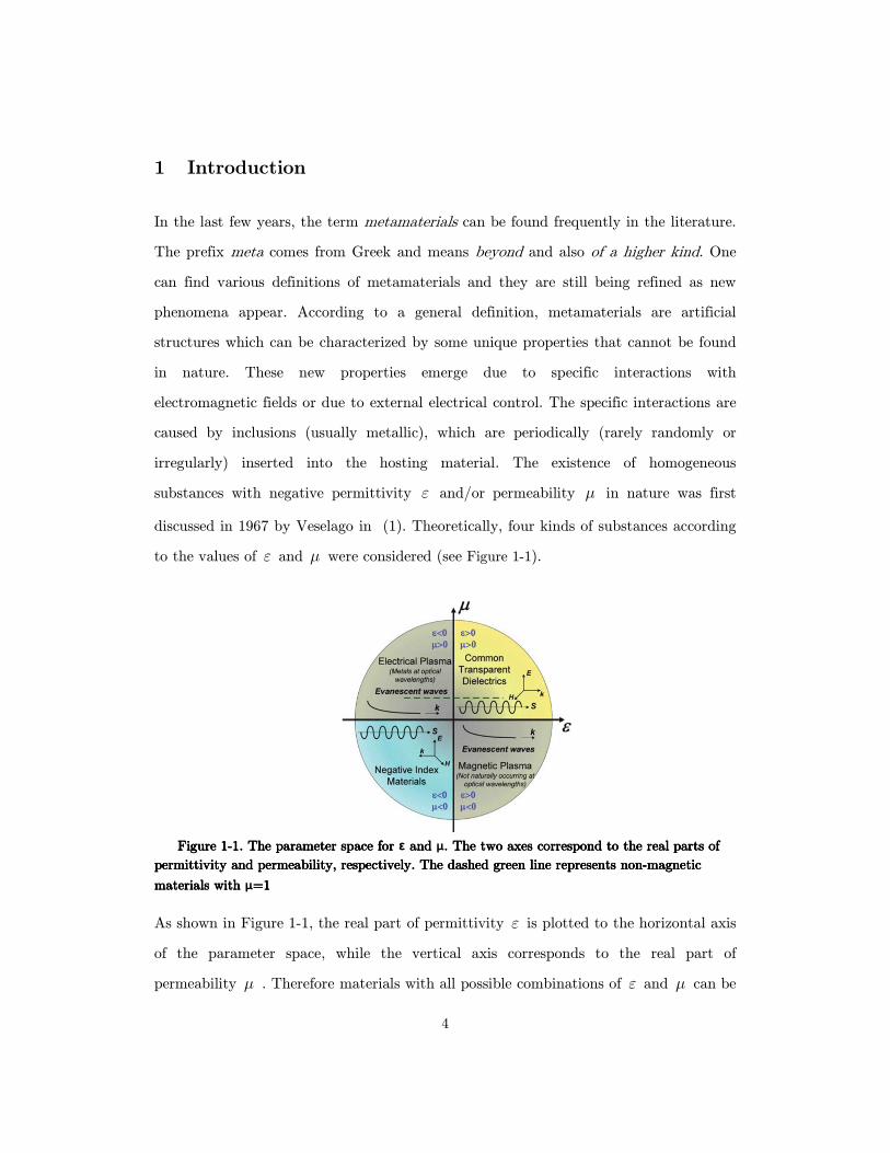
discussed in 1967 by Veselago in (1). Theoretically, four kinds of substances according

to the values of ε and µ were considered (see Figure 1-1).

Figure Figure Figure Figure 1111----1111. . . . The parameter space for The parameter space for The parameter space for The parameter space for ε and and and and μ. The two axes correspond to the real parts of . The two axes correspond to the real parts of . The two axes correspond to the real parts of . The two axes correspond to the real parts of

permittivity and permeability, respectively. The dashed green line represents nonpermittivity and permeability, respectively. The dashed green line represents nonpermittivity and permeability, respectively. The dashed green line represents nonpermittivity and permeability, respectively. The dashed green line represents non----magneticmagneticmagneticmagnetic

materials with materials with materials with materials with μ=1=1=1=1

As shown in Figure 1-1, the real part of permittivity ε is plotted to the horizontal axis

of the parameter space, while the vertical axis corresponds to the real part of

permeability µ . Therefore materials with all possible combinations of ε and µ can be

5

placed in the parameter space. Conventional materials known to be transparent are

found in the first quadrant, where both ε and µ have positive values. A negative

value of ε (µ ) indicates that the direction of the electric (magnetic) field induced

inside the material is in the opposite direction to the incident field. Noble metals at

optical frequencies are good examples for materials with negative ε , and negative µ

can be found in ferromagnetic media near a resonance (2). No propagating waves can

be supported in materials represented by the second and fourth quadrants, where one

of the two parameters is negative and the index of refraction becomes purely imaginary.

In the domain of optics, all conventional materials are confined to an extremely narrow

zone around a horizontal line at µ=1 in the space, as represented by the dashed line in

Figure 1-1. Moreover in an anisotropic medium, the field vectors EEEE and DDDD are not

necessarily parallel to each other; hence the permittivity must be in the form of a

tensor rather than a scalar value. Anisotropic and strongly dispersive features generally

occur in most of metamaterials studied thus far; for this reason, we should always

specify the frequency and direction under consideration when we address any effective

parameters in a metamaterial. Various kinds of passive artificial media are under

consideration, and these media can be divided into two large classes. In one of the

classes, the spatial period of the inclusions in the hosting material is small compared to

the wavelength. This means that the spatial dispersion effects are weak. In the other

case we have structures in which those characteristic sizes are comparable with the

wavelength known as photonic crystal (3). This is a situation of strong spatial

dispersion, and the usual material description in terms of its permittivity and

permeability loses its sense.

In (1) Veselago introduced the term left-handed materials for metamaterials. This term

is widely used today, but can have different meanings from different points of view (4)

(5). Several other names for these materials are also in use: mentioning that the term

metamaterial should be used for three-dimensional volumetric or bulk structures.

6

• Veselago media

• Media with simultaneously negative permittivity and permeability

• Double-negative(DNG) media

• Negative index of refraction (NIR or NRI) media

• Negative phase-velocity media

• Backward-wave (BW) media

• Left-handed (LH) media

Media with only one negative parameter are sometimes called single-negative

(SNG), specifically either ε -negative (ENG) or µ -negative (MNG) media. Many

authors use the term left-handed media. It should be noted that when we say

something is left- or right-handed, this term can have three different denotations in

electromagnetism:

• Right- or left-handed in structure of materials

• Right- or left-handed in polarization of the propagating media

• Right- or left-handed basis of the three vectors characterizing the wave

The first meaning comes from the basic sense: for example, the left hand cannot be

superimposed on the right hand by only making rotations and translations. They are

mirror images of each other. The Greek word gives us the term chiral for objects that

are right- or left-handed (e.g., screws). Chiral materials can be formed from chiral

objects: when one mixes left-handed objects into a neutral host medium the result is a

left-handed material. The well-known effect of chirality on wave propagation through

such a medium is that the polarization plane rotates along the propagation path (6).

Another meaning of right- or left-handed orientation is related to the polarization of

the electromagnetic wave, which is determined by the behaviour of the electric field

7

vector. Because there are two possibilities in the direction of the rotation, we come to

two choices of polarization: left-handed and right-handed. The orientation of the

polarization is dependent on the direction of observation. The third use of right- or left-

handed orientation is more abstract and is connected with the vector system associated

with wave propagation. In an “ordinary” medium with µ >0 and ε >0, the system (EEEE, HHHH,

kkkk) forms a right-handed triplet, whereas if ε and µ are negative, the triplet is left-

handed. For such media, the propagation constant kkkk is opposite to the power flow.

From these examples it is obvious that the widely used term left-handed is not very

suitable for metamaterials. The term gives the impression that the right- or left-handed

orientation is a characteristic of the material itself, which generally is not true.

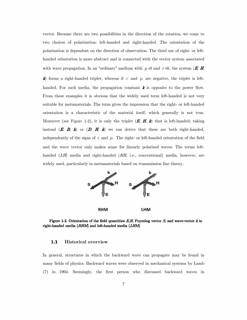
Moreover (see Figure 1-2), it is only the triplet (EEEE, HHHH, kkkk) that is left-handed; taking

instead (EEEE, BBBB, kkkk) or (DDDD, HHHH, kkkk) we can derive that these are both right-handed,

independently of the signs of ε and µ . The right- or left-handed orientation of the field

and the wave vector only makes sense for linearly polarized waves. The terms left-

handed (LH) media and right-handed (RH, i.e., conventional) media, however, are

widely used, particularly in metamaterials based on transmission line theory.

Figure Figure Figure Figure 1111----2222. Orientation of the field quantities . Orientation of the field quantities . Orientation of the field quantities . Orientation of the field quantities EEEE,,,,HHHH, Poynting vector , Poynting vector , Poynting vector , Poynting vector SSSS, and wave, and wave, and wave, and wave----vector vector vector vector kkkk in in in in

rightrightrightright----handed media (handed media (handed media (handed media (RHMRHMRHMRHM) and left) and left) and left) and left----handed media (handed media (handed media (handed media (LHMLHMLHMLHM))))

1.11.11.11.1 Historical overview

In general, structures in which the backward wave can propagate may be found in

many fields of physics. Backward waves were observed in mechanical systems by Lamb

(7) in 1904. Seemingly, the first person who discussed backward waves in

8

electromagnetism was Schuster (8). He briefly noted Lamb’s work and gave a

speculative discussion of its implications for optical refraction, when a material with

such properties were to be found. Around the same time, Pocklington (9) showed that

in a specific backward-wave medium a suddenly activated source produces a wave

whose group velocity is directed away from the source, while its phase velocity moves

toward the source. In electromagnetism, metamaterials are characterized by negative

permittivity and permeability. One of the first references to substances with negative

material parameters comes from Mandelshtam (10), who proposed the idea of the

reversed Snell’s law. The possibility of negative phase velocity of an electromagnetic

wave was predicted by Sivukhin (11). He observed that media with negative

parameters are backward-wave media, but had to state that “media with ε <0 and µ <0

were not known. The question of the possibility of their existence was not clarified.”

The first more extensive paper on hypothetical materials with negative permittivity

and permeability was introduced by Veselago (1). For centuries people had believed

that the refraction index can only be positive, but in this paper it was suggested that it

could also be negative. The term left-handed material was used for the first time there.

In the case of µ 0> and, 0ε > the vectors EEEE, HHHH and kkkk form a right-handed triplet,

and if 0µ < and 0ε < , they form a left-handed set as just pointed above. Since

vector kkkk is in the direction of the phase velocity, it is clear that left-handed substances

are substances with negative group velocity, which occurs in particular in anisotropic

substances or when there is spatial dispersion. In (1), several examples are discussed,

including the reversed Doppler effect, the reversed Vavilov-Cerenkov effect, and the

refraction of a ray at the boundary between left-handed and conventional media.

Veselago introduced the term rightness, which can be positive or negative, to divide

materials into two categories: right-handed and left-handed. The question of the proper

use of the term left-handed was discussed above.

9

Figure Figure Figure Figure 1111----3333. Refraction at two. Refraction at two. Refraction at two. Refraction at two----medium interface as determined bymedium interface as determined bymedium interface as determined bymedium interface as determined by phase matphase matphase matphase matcccching.hing.hing.hing.

One way to understand negative refraction is through the idea of phase matching. To

illustrate, consider the two-medium interface of Figure 1-3, where medium 1 (M1 ) is an

RHM and medium 2 (M2) is unspecified for the moment. A plane wave originating in

M1 is incident on the interface with wave-vector k1, , , , and it establishes a refracted wave

in M2 with wave-vector k2 such that their tangential components k1t and k2t are equal,

according to the conservation of the wave momentum. Having specified the tangential

components, we immediately recognize that there are two possibilities for the normal

component of k2: : : : the first case, in which k2 is directed away from the interface, and the

second case, usually describing reflected waves, in which k2 is directed towards the

interface. These two cases are represented as Case 1 and Case 2 in Figure 1-3. By the

conservation of energy, the normal components of the Poynting vectors SSSS1111 and SSSS2222 must

remain in the positive z-direction through both media. Thus, Case 1 depicts the usual

situation in which M2 is a conventional positive-index medium; however, if M2 is a

medium supporting propagating backward waves (LHM), then the wave-vector kz must

be directed oppositely to the Poynting Vector SSSS2222 (i.e., with a normal component in the

negative z-direction). Therefore, refraction in media that support backward waves must

be described by the second case, in which power is propagated along the direction of

phase advance, , , , and so is directed through a negative angle of refraction. Thus, M2 can

be seen to possess an effectively negative refractive index.

10

1.21.21.21.2 The recent interest in metamaterial.

The paper published by Veselago in 1967 provoked considerable interest at the time.

Surprisingly, however, real metamaterial research did not start until about three

decades later, when several seminal papers were published. The idea of having negative

effective material parameters and thus a negative refractive index was stunning, but it

lacked practical applications. In 1999, Pendry et al. (12) showed that microstructures

built from nonmagnetic conducting sheets exhibit an effective magnetic permeability

effµ , which can be tuned to values not accessible in naturally occurring materials,

including large imaginary components of effµ . The microstructure is on a scale much

smaller than the wavelength of radiation, and is not resolved by incident microwave

radiation. An example of such a structure is an array of non-magnetic thin sheets of

metal, planar metallic split-rings or so called Swiss rolls (12). Using Swiss rolls, a very

strong magnetic response can be achieved. The idea of a material with a negative

refractive index was worked out by Smith in 2000 in the paper (13). There he drew

inspiration from Veselago’s paper and proposed an artificial material which can produce

both negative effective permittivity and negative effective permeability. Veselago had

been looking for such a material for many years, and had expended huge amounts of

time and resources, but unfortunately he did not find the proper way. He had intended

to build the metamaterial as a mixture of natural materials with electric and/or

magnetic anisotropy. The problem was always with high losses and the resonance of

magnetically and electrically anisotropic materials at different frequencies . The idea of

Smith et al. was different, since it utilized a composite material, not a homogeneous

one. One of the revolutionary metamaterial applications was proposed in 2000 by

Pendry in (14). It is well known that with a conventional optical lens the sharpness of

the image is always limited by the wavelength of light used for illuminating the object.

An unconventional alternative to a lens, a slab of negative refractive index material,

has the power to focus all Fourier components of a two-dimensional image, even those

that do not propagate (evanescent waves). The waves decay in amplitude, not in phase,

11

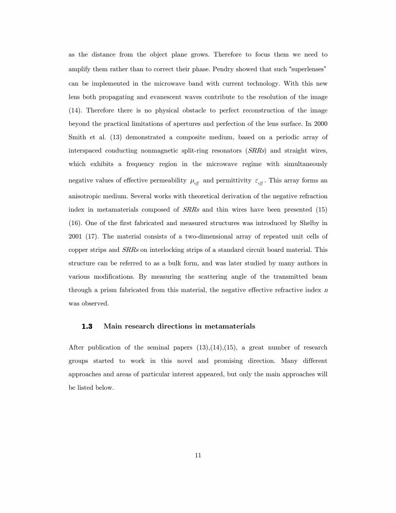
as the distance from the object plane grows. Therefore to focus them we need to

amplify them rather than to correct their phase. Pendry showed that such “superlenses”

can be implemented in the microwave band with current technology. With this new

lens both propagating and evanescent waves contribute to the resolution of the image

(14). Therefore there is no physical obstacle to perfect reconstruction of the image

beyond the practical limitations of apertures and perfection of the lens surface. In 2000

Smith et al. (13) demonstrated a composite medium, based on a periodic array of

interspaced conducting nonmagnetic split-ring resonators (SRRs) and straight wires,

which exhibits a frequency region in the microwave regime with simultaneously

negative values of effective permeability effµ and permittivity

effε . This array forms an

anisotropic medium. Several works with theoretical derivation of the negative refraction

index in metamaterials composed of SRRs and thin wires have been presented (15)

(16). One of the first fabricated and measured structures was introduced by Shelby in

2001 (17). The material consists of a two-dimensional array of repeated unit cells of

copper strips and SRRs on interlocking strips of a standard circuit board material. This

structure can be referred to as a bulk form, and was later studied by many authors in

various modifications. By measuring the scattering angle of the transmitted beam

through a prism fabricated from this material, the negative effective refractive index n

was observed.

1.31.31.31.3 Main research directions in metamaterials

After publication of the seminal papers (13),(14),(15), a great number of research

groups started to work in this novel and promising direction. Many different

approaches and areas of particular interest appeared, but only the main approaches will

be listed below.

12

1.3.1 Negative permittivity

It is well known that plasmas are described by a permittivity function that becomes

negative below a plasma frequency pω , causing the propagation constant in the

plasma to become imaginary. In this frequency region, electromagnetic waves incident

on the plasma suffer reactive attenuation and are reflected. Thus, the plasma frequency

bears a resemblance to the modal cutoff frequencies of particular electromagnetic

waveguides, below which the waveguide environment can be perceived as an inductively

loaded free space, as observed in 1954 by R. N. Bracewell (18). The idea of modeling

plasmas using artificial dielectrics was examined as early as 1962 by Walter Rotman

(19). His analysis, however, could not explicitly consider the permittivity of the media

and, instead, was limited to the consideration of their index of refraction. Rotman

noted that an isotropic electrical plasma could be modeled by a medium with an index

of refraction below unity, provided that its permeability was near that of free space.

Consequently, the sphere and disk-type media were excluded, since the finite

dimensions of these conducting inclusions transverse to the applied electric field give

the effective medium a diamagnetic response. What remained was the “rodded”

dielectric medium, or conducting strip medium, consisting of thin wire rods oriented

along the incident electric field. The dispersion characteristics of this medium showed

that it does, indeed, behave like a plasma. The idea of a negative permittivity was

implicit in many such works, but it was not until nearly a quarter-century later, when

Rotman’s rodded dielectric was rediscovered, that it was made clear exactly how a wire

medium resembled a plasma. It is evident that in the construction of electromagnetic

structures of any sort in the microwave range, we rely on the properties of metals.

Essentially, metals are plasmas, since they consist of an ionized “gas” of free electrons.

Below their plasma frequency, the real component of the permittivity of bulk metals

can be said to be negative. However, the natural plasma frequencies of metals normally

occur in the ultraviolet region of the electromagnetic spectrum, in which wavelengths

are extremely short. This condition certainly precludes the use of realizable artificial

13

dielectrics in the microwave range, which, moreover, must operate in the long

wavelength regime. Although the permittivity is negative at frequencies below the

plasma frequency, the approach toward absorptive resonances at lower frequencies

increases the dissipation, hence the complex nature of ε . Thus, to observe a negative

permittivity with low absorption at microwave frequencies, it would be necessary to

somehow depress the plasma frequency of the metal. This problem was addressed by

Pendry et al. (20) (and simultaneously by Sievenpiper et al. (21)), who proposed the

familiar structure of Rotman consisting of a mesh of very thin conducting wires

arranged in a periodic lattice, but approached the problem from a novel standpoint.

Due to the spatial confinement of the electrons to thin wires, the effective electron

concentration in the volume of the structure is decreased, which also decreases the

plasma frequency. More significant, however, is that the self-inductance of the wire

array manifests itself as a greatly enhanced effective mass of the electrons confined to

the wires. This enhancement reduces the effective plasma frequency of the structure by

many orders of magnitude, placing it well into the gigahertz range. Thus, an array of

thin metallic wires, by virtue of its macroscopic plasma-like behavior, produces an

effectively negative permittivity at microwave frequencies.

1.3.2 Negative permeability

Before dismissing the possibility of achieving 0µ < using natural isotropic substances,

Veselago momentarily contemplated the nature of such a substance. He imagined a gas

of magnetic “charges” exhibiting a magnetic plasma frequency, below which the

permeability would assume negative values. The obstacle, of course, was the

constitutive particle itself, the hypothetical magnetic charge. It is important to note

that in the effort to synthesize a negative effective permittivity, Rotman and Pendry

relied on the analogies their structures shared with the simplified electrodynamics of

natural substances. Indeed, as acknowledged by Veselago himself (1), it is a much more

14

difficult task to synthesize an isotropic negative permeability, for which there exists no

known electrodynamics precedent.

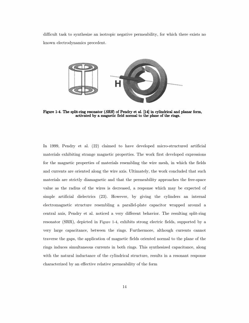
Figure Figure Figure Figure 1111----4444.... The splitThe splitThe splitThe split----ring resonator (ring resonator (ring resonator (ring resonator (SRRSRRSRRSRR) of Pendry et al. ) of Pendry et al. ) of Pendry et al. ) of Pendry et al. [14] [14] [14] [14] in cylindrical and planar form,in cylindrical and planar form,in cylindrical and planar form,in cylindrical and planar form, activated by a magnetic field normal to the plane of the activated by a magnetic field normal to the plane of the activated by a magnetic field normal to the plane of the activated by a magnetic field normal to the plane of the rings.rings.rings.rings.

In 1999, Pendry et al. (22) claimed to have developed micro-structured artificial

materials exhibiting strange magnetic properties. The work first developed expressions

for the magnetic properties of materials resembling the wire mesh, in which the fields

and currents are oriented along the wire axis. Ultimately, the work concluded that such

materials are strictly diamagnetic and that the permeability approaches the free-space

value as the radius of the wires is decreased, a response which may be expected of

simple artificial dielectrics (23). However, by giving the cylinders an internal

electromagnetic structure resembling a parallel-plate capacitor wrapped around a

central axis, Pendry et al. noticed a very different behavior. The resulting split-ring

resonator (SRR), depicted in Figure 1-4, exhibits strong electric fields, supported by a

very large capacitance, between the rings. Furthermore, although currents cannot

traverse the gaps, the application of magnetic fields oriented normal to the plane of the

rings induces simultaneous currents in both rings. This synthesized capacitance, along

with the natural inductance of the cylindrical structure, results in a resonant response

characterized by an effective relative permeability of the form

15

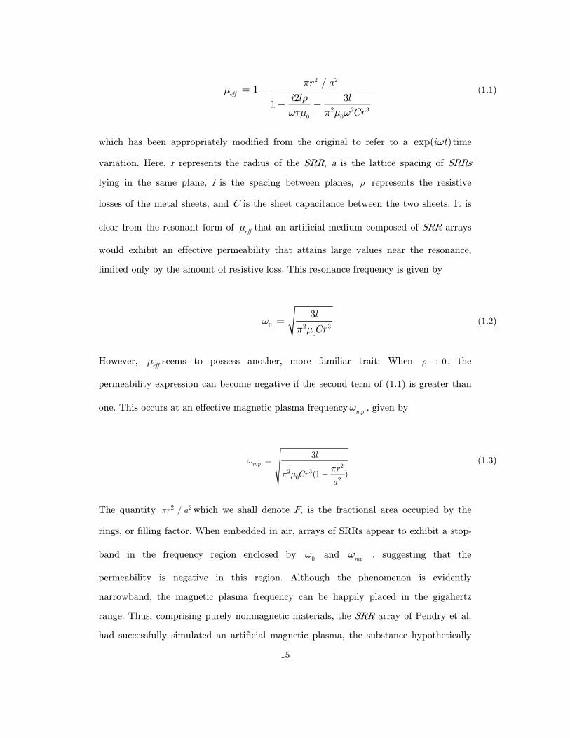
2 2

2 2 30 0

/1

2 31

eff

r a

i l l

Cr

πµ

ρ

ωτµ π µ ω

= −

− −

(1.1)

which has been appropriately modified from the original to refer to a exp( )i tω time

variation. Here, r represents the radius of the SRR, a is the lattice spacing of SRRs

lying in the same plane, l is the spacing between planes, ρ represents the resistive

losses of the metal sheets, and C is the sheet capacitance between the two sheets. It is

clear from the resonant form of effµ that an artificial medium composed of SRR arrays

would exhibit an effective permeability that attains large values near the resonance,

limited only by the amount of resistive loss. This resonance frequency is given by

0 2 3

0

3l

Crω

π µ= (1.2)

However, effµ seems to possess another, more familiar trait: When 0ρ → , the

permeability expression can become negative if the second term of (1.1) is greater than

one. This occurs at an effective magnetic plasma frequencympω , given by

2

2 30 2

3

(1 )

mp

l

rCr

a

ωπ

π µ

=

−

(1.3)

The quantity 2 2/r aπ which we shall denote F, is the fractional area occupied by the

rings, or filling factor. When embedded in air, arrays of SRRs appear to exhibit a stop-

band in the frequency region enclosed by 0ω and

mpω , suggesting that the

permeability is negative in this region. Although the phenomenon is evidently

narrowband, the magnetic plasma frequency can be happily placed in the gigahertz

range. Thus, comprising purely nonmagnetic materials, the SRR array of Pendry et al.

had successfully simulated an artificial magnetic plasma, the substance hypothetically

16

envisioned by Veselago, for which the effective permeability assumes negative values at

microwave frequencies. The role of the magneto-electric coupling in SRRs can be

minimized by the proper choice of geometrical dimensions or by applying symmetries in

the design, but some residual coupling still remains. A method for calculation and

measurement of the magneto-electric coupling (bianisotropy) of SRRs is proposed in

(24) (25). The possibility of designing isotropic 3D magnetic resonators by properly

arranging modified SRRs was studied in .

1.3.3 Perfect lens

From optics it is well known that no lens can focus light on an area smaller than the

square wavelength, thus it is not able to provide an image of objects smaller than the

wavelength of the light illuminating the object. The hypothetical perfect lens overcomes

this rule. Unlike conventional optical components, it will focus both the propagating

spectra and the evanescent waves, and thus be capable of achieving diffraction-free

imaging. In 2000, Pendry (14) predicted an intriguing property of such a LH lens (later

refined in (26), (27), a solution of a spherical perfect lens was given in (28)). Such a

lens is formed by a planar slab of double-negative material. Currently, samples of

double-negative materials are created mainly in the microwave region (29), (30), (31),

(32) due to the difficulty of achieving a strong magnetic response at higher frequencies.

Planar lenses, however, can operate only when the source is close to the lens (the

distance is related with the slab thickness). For practical applications, such as

telescopes and microwave communications, distant radiation needs to be focused. In

order to focus far field radiation, the negative refractive index (NRI) lens with a

concave surface is generally used. The monochromatic imaging quality of a

conventional optical lens can be characterized by the five Seidel aberrations: spherical,

coma, astigmatism, field curvature, and distortion. In (33), aberrations in a general

NRI concave lens have been studied by Smith and Schurig. They found that this lens

allows reduction or elimination of more aberrations than can be achieved with only

17

positive refractive index media. The 3D superresolution in metamaterial slabs was

experimentally shown in (34), and the theory was later generalized to an arbitrary

subdiffraction imaging system (35). The sensitivity of NRI lens resolution to the

material imperfection is studied in (36). The creation of left-handed materials at THz

frequencies and in the optical range meets with problems in getting the required

magnetic properties (37) (38), which have to be created artificially. In the absence of

magnetic properties, the lenses formed by materials with negative permittivity only (for

example, silver at optical frequencies (14), (39) or an array of metallic nanorods (40))

are still able to create images with subwavelength resolution, but the operation is

restricted to p-polarization only and the lens has to be thin as compared to the

wavelength. This idea was confirmed by experimental results (41), which demonstrated

the reality of subwavelength imaging using silver slabs in the optical frequency range.

The resolution of such lenses is restricted by losses in the silver. At the present time

there is no recipe for increasing the thickness of such lenses other than the introduction

of artificial magnetism.

1.3.4 Metamaterials cloaks

Another interesting practical application of metamaterials is a cloaking device. Let us

imagine an object covered by a hypothetical material which is able to bend the

electromagnetic waves passing through so that they go around the object and then

return undisturbed to their original trajectories. Then for an observer outside it seems

that the object is “invisible”. The idea was first suggested by Pendry et al. in (42) and

then elaborated in (43) where spherical and cylindrical cloaks were worked out. The

authors described a method in which the transformation properties of Maxwell

equations and the constitutive relations can yield material descriptions that allow such

manipulations with the beam trajectory. Leonhardt described a similar method, where

the two-dimensional Helmholtz equation is transformed to produce similar effects in the

geometric limit (44). Probably the first practical realization of a two-dimensional

cloaking device was demonstrated under certain approximations in (45). A copper

18

cylinder was “hidden” inside a cloak constructed with the use of artificially structured

metamaterials, designed for operation over a band of microwave frequencies. The cloak

decreases the scattering from the hidden object while at the same time reduces its

shadow, so that the cloak and object combined begin to resemble empty space. No real

three-dimensional cloaking device has been fabricated so far.

1.3.5 Chiral and bi-anisotropic materials

Chiral media provide another example of metamaterials with promising properties

(6). In chiral media, the spatial geometrical character of the internal structure (anti-

symmetry or non-symmetry with respect to the mirror reflection) rotates the

polarization of the propagating plane wave. This rotation is due to the magneto-electric

coupling caused by chiral elements. The bianisotropy of SRRs was studied in (46). A

way to obtain negative refraction with chiral materials was proposed by Pendry in (47)

and later extended by several research groups, see, e.g., (48), (49), (50), (51), (52). The

advantage of these structures is that they can provide both negative effective

permittivity and negative effective permeability with just one particle instead of the

two (e.g., SRRs and wires) needed in conventional metamaterials.

1.3.6 Tunable metamaterials

Most of the practical metamaterial implementations so far have been narrow-band

resonant structures. No wonder that researchers would like to achieve more broadband

and tunable devices. Metamaterial applications can be divided into two big groups: the

first one usually uses active devices to tune the capacitance or inductance in order to

achieve left-handed behavior in various frequency bands (varactor-loaded split-ring

resonators (53) coupled to micro-strip lines can lead to metamaterial transmission lines

with tuning capability (54), a tunable impedance surface etc.. whereas the other group

utilizes generally anisotropic natural materials with properties that are dependent on

19

external electric or magnetic field intensity. Such examples are nonlinear dielectric

substrates (55), tunable phase shifters based on ferroelectric films (56) which have

properties dependent on external fields. Utilization of micro-electro-mechanical

structures (MEMS) as tunable capacitors is shown in (57). Another extensive class of

tunable metamaterials is formed by liquid crystals. The properties of liquid crystals can

be changed easily by applying an external electric field. Hence, they are adaptable for

tuning. Bush and John (58) predicted the tunability of the band structure in photonic

crystals utilizing liquid crystals. Takeda and Yoshino (59) showed tunable refraction

effects in photonic crystal structures infiltrated by liquid crystals.

Recently (60) was analyzed numerically the optical response and effective macroscopic

parameters of Fishnet metamaterials infiltrated with a nematic liquid crystal which

enables switchable optical metamaterials, where the refractive index can be switched

from positive to negative by an external field.

1.3.7 Optic metamaterials.

The idea of metamaterials has been quickly adopted even to THz and optical

frequencies, since nanofabrication and sub-wavelength imaging have developed rapidly

in recent years. When the light interacts with a conventional material, then from the

electric and magnetic component of the light only the electric component probes the

atoms of a material effectively whereas the interaction with the magnetic component is

usually weak. However, metamaterials allow both components of the light to be

coupled, when they are designed properly. This can lead to fascinating applications

such as super-lenses, optical nanolithography, ”invisibility cloaks” etc. The

metamaterials known from microwave frequencies, however, are difficult to fabricate at

optical frequencies. For materials at optical frequencies, the dielectric permittivity ε is

very different from that in a vacuum, whereas the magnetic permeability µ (for

natural materials) is close to that in a vacuum. This is because of the weak interaction

with the magnetic component of the light, mentioned above (61). Conventional SRRs

operating at GHz frequencies were scaled down up to 1 THz frequencies (62), and

20

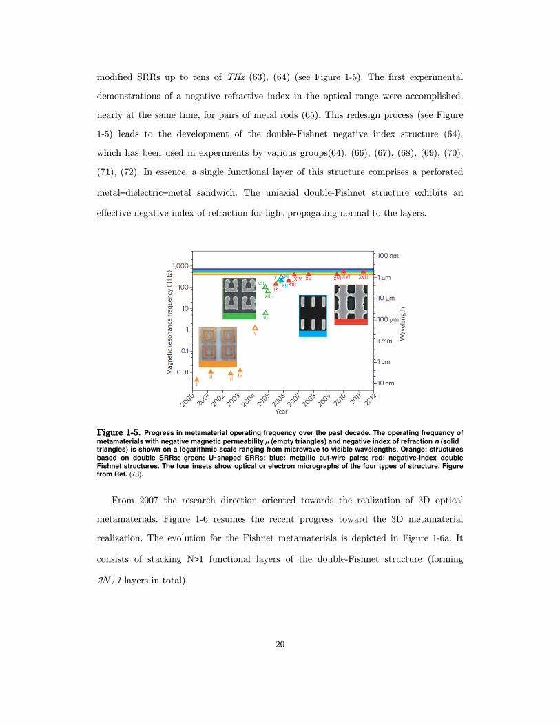
modified SRRs up to tens of THz (63), (64) (see Figure 1-5). The first experimental

demonstrations of a negative refractive index in the optical range were accomplished,

nearly at the same time, for pairs of metal rods (65). This redesign process (see Figure

1-5) leads to the development of the double-Fishnet negative index structure (64),

which has been used in experiments by various groups(64), (66), (67), (68), (69), (70),

(71), (72). In essence, a single functional layer of this structure comprises a perforated

metal–dielectric–metal sandwich. The uniaxial double-Fishnet structure exhibits an

effective negative index of refraction for light propagating normal to the layers.

Figure Figure Figure Figure 1111----5555. . . . Progress in metamaterial operating frequency over the past decade. The operating frequency of

metamaterials with negative magnetic permeability µ (empty triangles) and negative index of refraction n (solid triangles) is shown on a logarithmic scale ranging from microwave to visible wavelengths. Orange: structures

based on double SRRs; green: U‑‑‑‑shaped SRRs; blue: metallic cut-wire pairs; red: negative-index double Fishnet structures. The four insets show optical or electron micrographs of the four types of structure. Figure from Ref. (73).

From 2007 the research direction oriented towards the realization of 3D optical

metamaterials. Figure 1-6 resumes the recent progress toward the 3D metamaterial

realization. The evolution for the Fishnet metamaterials is depicted in Figure 1-6a. It

consists of stacking N>1 functional layers of the double-Fishnet structure (forming

2N+1 layers in total).

21

Figure Figure Figure Figure 1111----6666.Fig 3D photo.Fig 3D photo.Fig 3D photo.Fig 3D photonicnicnicnic----metamaterialmetamaterialmetamaterialmetamaterial structures. (astructures. (astructures. (astructures. (a) Double) Double) Double) Double----FishnetFishnetFishnetFishnet negativenegativenegativenegative----index index index index

metamaterialmetamaterialmetamaterialmetamaterial with several layers. (bwith several layers. (bwith several layers. (bwith several layers. (b) ) ) ) ‘StereoStereoStereoStereo’ or chiral or chiral or chiral or chiral metamaterialmetamaterialmetamaterialmetamaterial fabricated through stackfabricated through stackfabricated through stackfabricated through stacked ed ed ed

electronelectronelectronelectron----beam lithography. (cbeam lithography. (cbeam lithography. (cbeam lithography. (c) Chiral ) Chiral ) Chiral ) Chiral metamaterialmetamaterialmetamaterialmetamaterial made using directmade using directmade using directmade using direct----laslaslaslaser writing and er writing and er writing and er writing and

electroplatinelectroplatinelectroplatinelectroplating g g g . (d. (d. (d. (d) Hyperbolic (or ) Hyperbolic (or ) Hyperbolic (or ) Hyperbolic (or ‘indefiniteindefiniteindefiniteindefinite’) ) ) ) metamaterialmetamaterialmetamaterialmetamaterial made by electroplating hmade by electroplating hmade by electroplating hmade by electroplating hexagonalexagonalexagonalexagonal----

holeholeholehole----array templates array templates array templates array templates . (e. (e. (e. (e) Metal) Metal) Metal) Metal–dielectric layered dielectric layered dielectric layered dielectric layered metamaterialmetamaterialmetamaterialmetamaterial composed of coupled plasmonic composed of coupled plasmonic composed of coupled plasmonic composed of coupled plasmonic

waveguides, enabling anglewaveguides, enabling anglewaveguides, enabling anglewaveguides, enabling angle----independent negative nindependent negative nindependent negative nindependent negative n for particular frequencies. for particular frequencies. for particular frequencies. for particular frequencies. (f(f(f(f)))) SRRs oriented SRRs oriented SRRs oriented SRRs oriented

in all three dimensions, fabricated using mein all three dimensions, fabricated using mein all three dimensions, fabricated using mein all three dimensions, fabricated using membrane projection lithography mbrane projection lithography mbrane projection lithography mbrane projection lithography . (g. (g. (g. (g) Wide) Wide) Wide) Wide----angle angle angle angle

visible negativevisible negativevisible negativevisible negative----index index index index metamaterialmetamaterialmetamaterialmetamaterial based on a coaxial design based on a coaxial design based on a coaxial design based on a coaxial design . (h) Connected cubic. (h) Connected cubic. (h) Connected cubic. (h) Connected cubic----symmetry symmetry symmetry symmetry

negativenegativenegativenegative----index index index index metamaterialmetamaterialmetamaterialmetamaterial structure amenstructure amenstructure amenstructure amenable to direable to direable to direable to direct laser writingct laser writingct laser writingct laser writing. (i. (i. (i. (i) Metal cluster) Metal cluster) Metal cluster) Metal cluster----ofofofof----

clusters visibleclusters visibleclusters visibleclusters visible----frequency magnetic frequency magnetic frequency magnetic frequency magnetic metamaterialmetamaterialmetamaterialmetamaterial made umade umade umade using largesing largesing largesing large----area selfarea selfarea selfarea self----assembly assembly assembly assembly . (. (. (. (llll) All) All) All) All----

dielectric negativedielectric negativedielectric negativedielectric negative----index index index index metamaterialmetamaterialmetamaterialmetamaterial composed of twcomposed of twcomposed of twcomposed of two sets of higho sets of higho sets of higho sets of high----refractiverefractiverefractiverefractive----index index index index dielectric dielectric dielectric dielectric

spheres arraspheres arraspheres arraspheres arranged on a simpnged on a simpnged on a simpnged on a simplelelele----cubic latticecubic latticecubic latticecubic lattice. Figure taken from Ref.(73). Figure taken from Ref.(73). Figure taken from Ref.(73). Figure taken from Ref.(73)

1.41.41.41.4 The aim of the thesis

The general aim of this work is to study the propagation of electromagnetic waves in

periodic structures, namely in “fish-net” like metamaterial structures (see structure

depicted in Figure 1-6a). It is well known that, when wavelengths much larger than

the periodicity cross these artificial systems, they can enable uncommon properties such

as the negative refraction index and the negative phase advance respect to the power

flow direction. The purpose of this thesis is to study the origin of the negative

refraction and its dependence on the geometric parameters of the structures. An

average method for the extraction of the effective parameters and the introduction of a

simple LC circuit formalism is commonly adopted for the investigation and some

clarification about the refractive index behavior under a parametric variation of the

fishnet. However this effective approaches to metamaterials are sometime insufficient to

22

explain the intrinsic nature of such structures being strictly related to their complex

dispersions. For this reason a robust approach toward the microscopic investigation of

periodic structures is presented and for the first time it is also extended to the case of

plasmonic/photonic crystal slabs. Within this (FEM) modal method based on the weak

form of the Elmholtz’s equation one can accurately extract all the complex Bloch-modes

of an elettromagnetic periodic system thus leading to the possibility of calculating the

modes losses. The method offers great reliability in computational time, extraction of

complex kkkk-bands, independence by any shape of periodic holes and kind of materials,

extraction of complex isofrequency contours, for either 2D periodic photonic/plamonic

crystal slabs or 2D-3D photonic/plamonic crystals. The thesis can be resumed as fellow:

the introduction gives a brief historical overview of metamaterial research, and the

main research directions in this area are outlined. The first part of the thesis

summarize the theoretic framework for the investigation of the average properties of

metamaterials. In the second part we report a design and a parametrical analysis of a

Fishnet in the optical spectral range. In particular the dependence of both the magnetic

and the electric resonance on the geometric features of the Fishnet is investigated in

the optical frequency spectrum. The transmission and reflection coefficients and

distribution of the electric field within the lattice were calculated by means of FEM

electromagnetic simulations. Moreover the properties of Fishnet metamaterial have

been investigated for a multi-layered structure. The SPPs modes propagating inside the

stacked metamaterial have been identified and enumerated. We show that the

asymptotic bulk properties for a multilayered Fishnet metamaterial are easily reached

by staking just more than 3-functional layers along the propagation direction. The

third part of the thesis reports a preliminary result on the nanofabrication of Fishnet

type Au/dieletric/Au metamaterial stacks. Nano-hole arrays have been realized on

Au(30 nm)-dielectric(50nm)-Au(30nm)/ITO stacks by means of direct ion milling with

FIB using a FEI Nova 600i instrument. Finite element method simulations were used

to design the structures and to foresee their optical behavior. The bianisotropic

approach for a more accurate extraction of the physical parameters is presented. In the

last part of the thesis a FEM modal method based on the weak form of the Helmholtz’s

23

equation is presented. The dispersion characteristic of plasmonic/photonic crystals in

the shape of a periodic slabs or of a 2D-3D periodic structure are calculated and the

method is applied on a Fishnet metamaterial. The complex kkkk-band diagrams are

calculated together with the isofrequency dispersion curves. The method allows the

identification of the left-handed modes and the calculation of losses in metal. The

simulation of the negative refraction from a NRI prism in the shape of a wedge is also

showed. The electric and magnetic modes generating the NRI are than identified with

plamonic resonances originating by the coupling of the incident momentum light with

the grating diffractive orders. In Chapter 5 a preliminary fabricated sample of Fishnet

metamaterial is reported. Moreover the presence of bianisotropy (always present in

fabricated sample) is studied by means of scattering parameters. In Chapter 6 and 7 a

powerful modal method based on weak formulation within the FEM environment is

reported. This method represent a very useful tool for the investigation of photonic and

plamonic structures allowing for the extraction of the complex photonic and plamonic

dispersion curves of the Bloch-modes.

24

2 Effective method approach to metamaterials

Materials composed of small elements are known to respond as continuous

media when the operating wavelength is much larger than the individual constituents.

A classic example of such materials are natural dielectrics that can be described by a

single parameter, the electric permittivity ε . All the negative and positive charges in a

dielectric medium are bound to their location by atomic forces and are therefore not

free to move like in a conductor. Under the influence of an external electric field,

however, these assemblies of negative and positive charges may slightly reorganize,

which results in the creation of bound electric dipoles. From a macroscopic point of

view, the orientation of these dipoles generates a polarization vector PPPP that influences

the electric flux density D D D D such as D D D D = 0ε EEEE+PPPP, where EEEE is the external applied

electric field. This allows one to define a general permittivity ε such that D D D D =ε 0ε EEEE,

where naturally ε is defined in terms of the polarization vector. Similarly, magnetic

media are described by a magnetic permeability µ , and ε and µ represent the

constitutive parameters essential to the macroscopic Maxwell equations. In our case,

the metamaterials are composite structures designed to exhibit specific electromagnetic

properties at some particular wavelengths that are much larger than the elementary

constituents. It is therefore legitimate to look for homogeneous or effective medium

parameters, typically an effective permeability. Like in the case of more standard

media, these constitutive parameters directly represent the properties of the medium:

isotropic metamaterials should be described by scalar constitutive parameters while

anisotropic ones should be described by second rank tensors ε and µ , losses induce

an imaginary part to these parameters, frequency dispersion yields frequency-dependent

parameters, non-locality makes them spatially dispersive (dependent on k), the passive

nature of metamaterials forces the imaginary parts to be positive, reciprocity imposes

conditions on the tensors, etc.

The homogenization procedure therefore involves two steps:

25

1. A hypothesis, more or less refined, on the characteristics of the medium

(isotropic vs. anisotropic, lossless vs. lossy, etc). Paradoxically, the properties of

the metamaterial are initially unknown, and yet a model has to be chosen to

perform the homogenization procedure. Therefore, the model should also be

tested a posteriori.

2. The determination (or retrieval) of the corresponding constitutive parameters

using numerical or analytical algorithms.

Once the overall model has been ascertained, the next step is to obviously determine

the numerical values of the components of the permittivity and permeability tensors.

The number of unknowns is directly related to the model chosen and dictates the

number of equations that must be obtained from measurements (either experimental

measurements or numerical simulations). For example, a simple lossy isotropic

dielectric material exhibits two unknowns, the real and imaginary parts of the scalar

permittivity, which can be obtained from one complex measurement such as the

reflection and/or the transmission coefficients.

Before detailing the homogenization procedures, it is necessary to say a few

words about the limitations of homogenization. Although we are interested

inhomogenizing metamaterials, the range of applicability of such process must be

carefully examined. In particular, homogenization would not be valid under the

following conditions:

1. When the constituents are not much smaller than the operating wavelength.

This includes metamaterials with unit cells large or comparable to wavelength

of the radiation, as well as dielectric photonic crystals operating close to hale

wavelength.

2. When the wave propagation inside the material cannot be described by a single

propagating mode. Such situation occurs for example close to the resonance of

some constituents of the metamaterials.

Failing to comply with these conditions may produce unphysical artifacts in the

frequency-dependent retrieved parameters, the most common of which are an anti-

26

resonance of the permittivity (with an associated negative imaginary part) at the

location of the resonance of the permeability (74), and possibly a truncated resonance

of the index of refraction as pointed out in Koschny et al.(2005). These artifacts have

been suggested to be due to the fact that the periodicity of the medium becomes visible

at the corresponding frequencies, making the homogenization hypothesis less accurate.

A conservative ratio of about 30 between the wavelength and the size of the unit cell

has been proposed for the homogenization hypothesis to be very well justified, although

most of the metamaterials realized to date exhibit a ratio of about 10 at best.

Typically one can deals with two distinct approach in order to determine the

constitutive parameters of an effective medium once: one consist on averaging the

internal fields over some relevant volume in the medium and the other is based on the

extraction from the reflection and transmission coefficients.

There are several methods based on the fields average more or less rigorous and

more or less valid under certain geometries and materials under study. The Maxwell-

Garnett approximation, which is essentially the quasi-static generalization of the

Clausius Mossotti electrostatic approximation, has been used widely to calculate the

bulk electromagnetic properties of inhomogeneous materials (75). The component with

the largest filling factor is considered to be a host in which other components are

embedded and the field induced in the uniform host by a single inclusion (assumed to

be spherical or elliptical) is calculated and the distortion of this field due to the other

inclusions is calculated approximately. The Maxwell–Garnett approach incorporates the

distortions due to the dipole field on an average and has been very successful in

describing the properties of dilute random inhomogeneous materials. There are other

effective medium theories (76), (77) for high filling fractions that include more residual

interactions or higher multi-pole effects. We should also note that there are more

mathematically rigorous homogenization theories (78), which analyses the fields in an

asymptotic expansion in terms of the microscopic length-scale associated with the

inhomogeneities, which is however beyond the scope of this doctoral thesis.

In the case of periodically structured materials,. the periodicity, first of all,

implies that the averaging need not be over orientational and density fluctuations.

27

Another approach (12) was first used to discretize Maxwell’s equations on a lattice

and it is essentially based on the fields averaging of the unit cell of the lattice (assumed

to be simple cubic).

The effective medium parameters determined from any such averaging process should

be unique and independent of the manner of the averaging process. Likewise, it should

give unique medium responses to applied fields, and it should be possible to uniquely

determine the scattered fields for the metamaterial. In fact, experiments usually access

only the emergent quantities such as the reflection and transmission through (say) a

slab of the effective medium and not the internal microscopic fields.

The method which will be more extensively presented is based on the extraction of the

complex materials parameters from the reflection and transmission coefficient and it is

traditionally overwhelmingly used in the metamaterial scientific community (79), (80),

(81), (82), (83), (84), (85).

This method is appealing because of its relative simplicity to set up in an experimental

configuration, as well as its numerical efficiency since the electromagnetic fields need

only to be computed over surfaces instead of volumes. In this procedure, the reflection

and transmission coefficients (R and T) are used as the linking information between the

incident electromagnetic field and the constitutive parameters, the latter relationship

being essentially the purpose of inversion or parameter retrieval algorithms.

2.12.12.12.1 The standard retrieval method

The first step is to determine the relationship between the incident, reflected,

and transmitted fields and the reflection/transmission coefficients. In order to comply

to the previous hypothesis, an effective medium is supposed to be of infinite extent in

the transverse x- and y-directions and of finite extent in the propagation z-direction.

We first assume that the medium is isotropic and homogeneous or symmetrically

inhomogeneous respect to the direction of propagation normal to the effective medium

slab. We illustrate the effective medium in Figure 2-1 indicated as region (2) embedded

in two air domains (region (1) and (3)). The single propagating mode here is taken to

be a plane wave, equivalent to the TEM mode in a parallel plate waveguide.

28

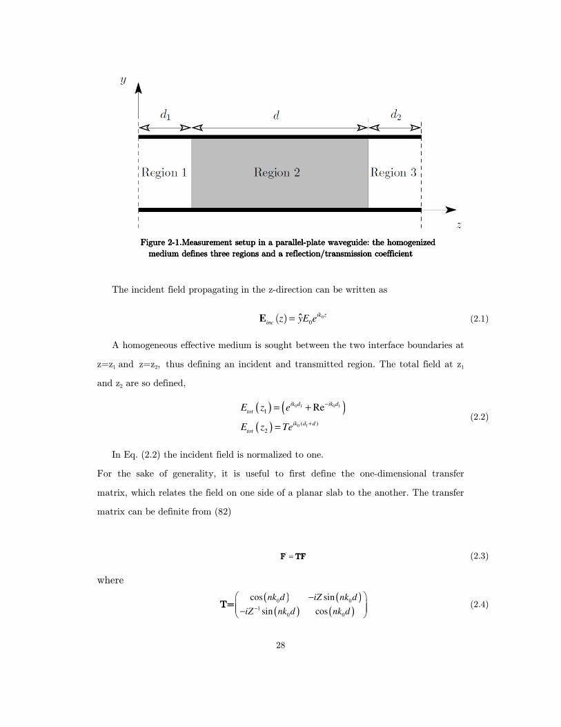
Figure Figure Figure Figure 2222----1111....Measurement setup in a parallelMeasurement setup in a parallelMeasurement setup in a parallelMeasurement setup in a parallel----plate waveguide: the homogenizedplate waveguide: the homogenizedplate waveguide: the homogenizedplate waveguide: the homogenized

medium defines three regions and a reflection/transmission coefficientmedium defines three regions and a reflection/transmission coefficientmedium defines three regions and a reflection/transmission coefficientmedium defines three regions and a reflection/transmission coefficient

The incident field propagating in the z-direction can be written as

0

0( ) ik z

incz yE e= ˆE (2.1)

A homogeneous effective medium is sought between the two interface boundaries at

z=z1 and z=z2, thus defining an incident and transmitted region. The total field at z1

and z2 are so defined,

( ) ( )( )

0 1 0 1

0 1

1

( )

2

Reik d ik d

tot

ik d d

tot

E z e

E z Te

−

+

= +

= (2.2)

In Eq. (2.2) the incident field is normalized to one.

For the sake of generality, it is useful to first define the one-dimensional transfer

matrix, which relates the field on one side of a planar slab to the another. The transfer

matrix can be definite from (82)

' =F TFF TFF TFF TF (2.3)

where

( ) ( )

( ) ( )0 0

1

0 0

cos sin

sin cosT=T=T=T=

nk d iZ nk d

iZ nk d nk d−

− −

(2.4)

29

is the T-matrix and

,1 ,2'

,1 ,2

F= , F = F= , F = F= , F = F= , F = E E

H H

t t

t t

(2.5)

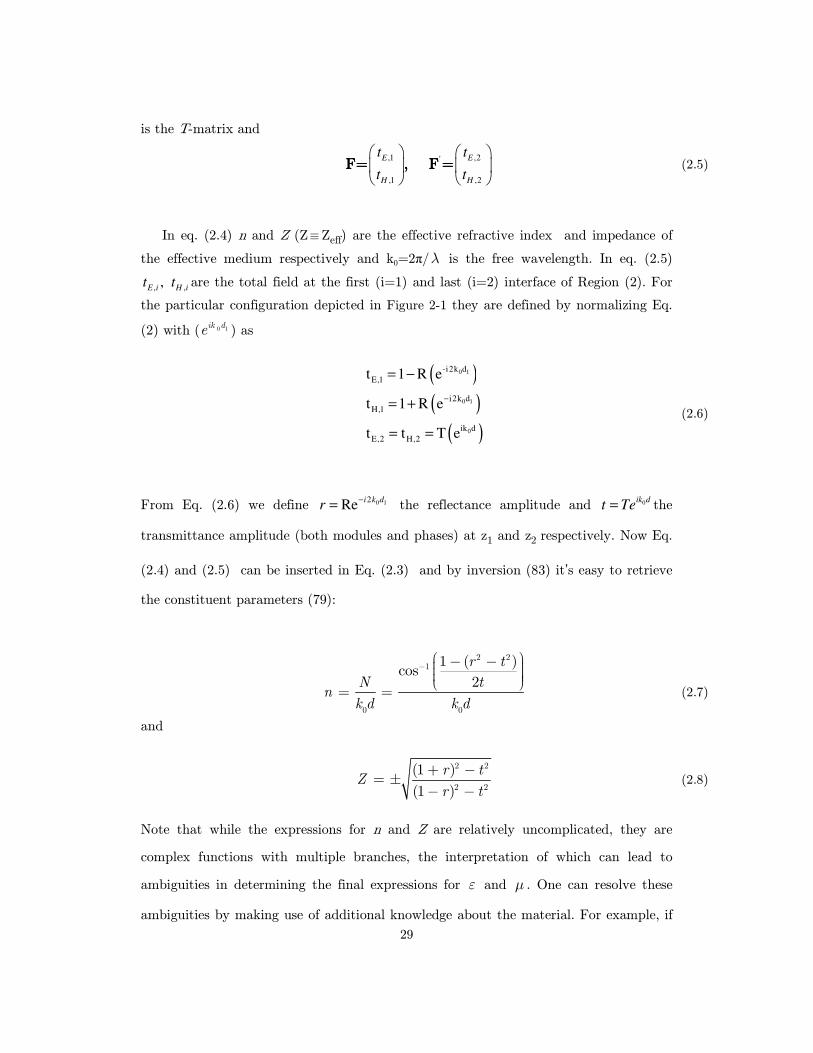
In eq. (2.4) n and Z (Z≡Zeff) are the effective refractive index and impedance of

the effective medium respectively and k0=2π/λ is the free wavelength. In eq. (2.5)

, ,,E i H it t are the total field at the first (i=1) and last (i=2) interface of Region (2). For

the particular configuration depicted in Figure 2-1 they are defined by normalizing Eq.

(2) with ( 0 1ik de ) as

( )( )

( )

0 1

0 1

0

-i2k d

E,1

i2k d

H,1

ik d

E,2 H,2

t 1 R e

t 1 R e

t t T e

−

= −

= +

= =

(2.6)

From Eq. (2.6) we define 0 12Re i k d

r−= the reflectance amplitude and 0ik d

t Te= the

transmittance amplitude (both modules and phases) at z1 and z2 respectively. Now Eq.

(2.4) and (2.5) can be inserted in Eq. (2.3) and by inversion (83) it’s easy to retrieve

the constituent parameters (79):

2 21

0 0

1 ( )cos

2

r t

tNn

k d k d

− − −

= = (2.7)

and

2 2

2 2

(1 )

(1 )

r tZ

r t

+ −= ±

− − (2.8)

Note that while the expressions for n and Z are relatively uncomplicated, they are

complex functions with multiple branches, the interpretation of which can lead to

ambiguities in determining the final expressions for ε and µ . One can resolve these

ambiguities by making use of additional knowledge about the material. For example, if

30

the material is passive, the requirement that Re(Z)>0 fixes the choice of sign in Eq.

(2.8). Likewise, Im(n)>0 leads to an unambiguous result for Re(n) and Im(n):

0Re( ) ' ( ( '') ' 2 ) / ( )n n sign N N l k dπ= = + (2.9)

0Im( ) '' ( '') ''/ ( )n n sign N N k d= = (2.10)

with the conditions

' 0

'' 0

Z

n

≥

≥ (2.11)

Where sign(x) is equal to 1 if 0x ≥ and to -1 otherwise and l is an integer number.

The branch factor is related to the number of wavelength that propagate inside the

slab. By choosing short samples, it is therefore possible to ensure that the sample is

smaller than one wavelength, thus automatically selecting m = 0 as solution. Such

strategy works well with standard dielectric, where the constitutive parameters are

usually reasonably small within the frequencies of interest and where their variations

with respect to frequency are small. In the case of left-handed media, however, the

parameters might take large absolute values, either at low frequencies for a Drude

model or close to resonance for a Lorentz model. Therefore, the small thickness of the

sample does not guarantee a sub-wavelength propagation distance due to the possibly

large values of the permittivity and the permeability (and hence the effective

wavelength inside the medium is small). A robust method for achieving the right

branch number has yet been proposed in (81) . Commonly when the number of layer in

the propagation direction consist of few elements in order to avoid ambiguities in

selecting a phase-adjusting integer l in Eq. (2.9) one should start the restoration of n’

from a higher wavelength (far away from resonances) and obtain physically sound

values of n’ . Then, the wavelength should be moved toward shorter values while

simultaneously adjusting the values of l in Eq. (2.9) to obtain a continuous behavior

for n’.

31

2.22.22.22.2 S-parameters

Scattering parameters (or S-parameters) are complex-valued, frequency dependent

matrices describing the transmission and reflection of electromagnetic energy measured

at different ports of devices like filters, antennas, waveguide transitions, and

transmission lines. The use of S-parameter is common in electromagnetic simulation

when one deals with a fundamental propagation mode which can be used to excite a

port with a known analytic profile. For homogeneous slab with small features and small

periodicity respect to the operative wavelength, the eigen-value associated to the

fundamental mode is an incident plane wave with incident power conventionally

normalized to one. S-parameters originate from transmission-line theory and are defined

in terms of transmitted and reflected voltage waves. For high-frequency problems,

voltage is not a well-defined entity, and it is necessary to define the scattering

parameters in terms of T-matrix. For homogeneous or symmetric homogeneous slab it

can be shown (82) that the S matrix is symmetric with:

( )

( )

( )

21 12

12 21

21 12

11 22

12 21

1

1

2

1

2 ,1

2

s

s

S S

T iT iT

i T TS S

T iT iT

= =

+ −

− += =

+ −

(2.12)

where 11 22sT T T= = . Using the analytic expression for the T-matrix elements in

Eq.(2.4) gives the S-parameters

( ) ( )21 12

1

1cos sin

2

S Si

nkd Z nkdZ

= = − +

(2.13)

and

( )11 22

1sin

2

iS S Z nkd

Z

= = − (2.14)

32

Equations (2.13) and (2.14) can be inverted to find n and Z in terms of the S-

parameters as follows:

( )1 2 211 21

21

1cos 1 ,

2N S S

S

− = − +

(2.15)

( )

( )

2 211 21

2 211 21

1

1

S SZ

S S

+ −=

− + (2.16)

The computation of the reflection and transmission coefficients in Eqs. (2.7)−(2.8) as

well as the computation of the S-parameters ins Eqs. (2.15), (2.16) requires the

knowledge of the scattered electromagnetic fields. Various numerical algorithms are

available toward this end, some of the most common ones being the Finite-Difference

Time-Domain Method (FDTD), Finite Element Method (FEM), the Transfer Matrix

Method, or an integral equation method such as the Method of Moments. The first

three methods have the appeal of an extreme generality and mathematical simplicity:

they have been applied for many years to solve a plethora of electromagnetic problems,

and are well documented in various references. Among this methods I’m aware only

with FEM and all the simulation have been performed by using the commercial FEM

software COMSOL Multyphysics @ (86). More detailed treatments can be found

elsewhere (87) , (88), (89). Eqs. (2.15), (2.16) are formally similar to Eq. (2.7), (2.8)

respectively and the same considerations about the determination of the integer l must

be careful token in mind. Moreover it’s important to stress that operatively the S-

parameters are defined at two boundaries at fixed distances (d=0 and d=d1+d+d2

respectively in our example) from the slab interfaces. For this reason it’s necessary to

de-embed the homogeneous slab from the cladding and substrate domains by

multiplying the S-parameters with constant phases (83):

00 1 0 1arg2 2

11 22 0

((E E )/E )|P tot inc in zii k d i k d

tot zS S re R e e=

−

== = = = (2.17)

and

0 1 2 0 1 2 2 0 1

2

arg (

21 12 ,E )|( ) ( ) ( )P out z d d

iik d d ik d d d ik d d

tot z dS S te Te e e=

+ + + +

== = = = (2.18)

33

Where Eout is the electric field and Ptot is the power flow calculated at the two outer

boundaries. The practical implementation of these equations for the retrieval of the

index of refraction and the impedance is hindered by a few issues that need to be

carefully examined :

1. The practical limitation of Eqs. (2.11)

2. The sensitivity of these parameters to noise

3. The definition of the material boundaries.

1. both numerical simulations and experimental measurements introduce perturbations

in the S parameters that translate into perturbations on n and Z. These perturbations

are typically small and can be filtered out unless the parameters themselves are close to

zero, in which case a small perturbation can induce an unphysical sign change. This

issue can be resolved by introducing a threshold in the use of Eqs. (2.11): when the

absolute value of Z is greater than the threshold, Eq. (2.11) can be used. Otherwise, the

sign of Z is determined such that the corresponding index of refraction has a non-

negative imaginary part. This condition is equivalent to 0 1ink de ≤ , where

0 21

11

11

1

ink d Se

ZS

Z

=−

−+

(2.19)

2. When the transmission is either close to zero or close to unity. In the first case,

which typically appears below the resonance band, S21 is close to zero which yields large

values in Eq. (2.15) and hence, strong variations in the index of refraction (seen as

unphysical spikes in the retrieved values). This situation is avoided by solving first for

the impedance. The latter is indeed stable as can be seen by inspecting the first

derivative

( )

221 11

2 221 11 21

8

1

S SZ

S S S

∂=

∂ − −

(2.20)

34

The second situation is the mirror of this first one: the impedance is unstable, whereas

the index of refraction is stable and should be used first in the retrieval process. Eqs.

(2.17),(2.18) can then be solved within a threshold.

3. The purpose of the homogenization procedure is to find the effective parameters of

metamaterials, but also to find the boundaries of the effective medium. The

metamaterials being usually composed of discrete metallic elements, it is not

immediately clear where these boundaries should be. The determination of the

boundaries can be performed based on the requirement of homogenization, namely that

the effective parameters of two slabs of different thicknesses should be identical at all

frequencies. This principle, along with the fact that the impedance depends on the slab

thickness, can be used to set up a minimization problem: the impedances of two

different metamaterial slabs are computed, and their difference is optimized across the

entire frequency spectrum of interest as function of the boundaries of the medium. The

boundaries that reach the minimum in a pre-defined sense are chosen to be the

boundaries of the effective medium. In the case of periodic structures, this method

yields the expected results that the effective boundaries coincide with the boundaries of

the unit cell of the metamaterial (81).

2.32.32.32.3 Retrieval method in presence of one or two substrate.

The retrieval method discussed thus far contains most of the essential physics for

extracting effective parameters from the amplitudes and phases of the waves

transmitted and reflected from a metamaterial slab. However, this technique is not

immediately applicable to most optical metamaterials, because the procedure is based

on the assumption that the metamaterial is in the form of a free-standing slab

surrounded by a vacuum. In almost all reported metamaterials for the optical

frequency, substrate layers are involved, and therefore the metamaterial slabs are

embedded in an asymmetric environment. In the most usual case one side of the

metamaterial slab is immediately attached to a microscopically thick substrate (usually

glass) and the other side interfaces air or vacuum. The NIM-air interface coefficients tE,1

35

and tH,1 are still defined by Eq.(2.6) but the coefficients at the NIM-substrate interface

are given by tE,2=t and tH,2=n2t and

( ) ( )

2 21 2

2 2

1cos ,

1 1

r n tN

n t rt n

− − + = + + −

(2.21)

where t is calculated (measured) in the substrate 0 2 2 1( )

21

ik n d dt S e− += , 0 12

11

i k dr S e−= and

n2≡nGlass.

Coefficients tE,1 and tH,1 at the NIM-air interface of a NIM layer on an ITO-glass

substrate are also defined by Eq.(2.6), but back side coefficients should be first

calculated (measured) in the substrate at the ITO-glass interface (tE,3=t and tH,3=n3t)

and then back-propagated using Eq. (2.4),

(2.22)

,2

2,2 3

,E

H

t tT

t n t

= (2.23)

where

( ) ( )( ) ( )

12 2 2

22 2 2

cos sin

sin cos

n kd in n kdT

in n kd n kd

− − = − (2.24)

with n2≡nITO, n3≡nGlass. After some algebra the effective parameters are the fellow:

( )( ) ( )

( )( ) ( )( )( )( ) ( )( )( )

1 2 22 2 0 2 3 2 2 2 2 0

2 2 0 2 2 2 0 2 3 2

2 2 0 3 2 2 0 2 3 2

cos 1 sin 2 / cos 2 /2

cos 1 sin /,

cos 1 sin /

iN r t n d k n n n n n d k

n d k n i n d k n n nt

r n d k n i n d k n n n

− = − + + +

+ + + + − + −

(2.25)

and

2 2 2

2 2 0 3 2 2 2 0

2 2 23 2 2 0 2 2 2 0

((1 ) (cos( ) ( / )sin( )) ),

((1 ) ( cos( ) sin( )) )

r t n d k i n n n d kZ

r t n n d k in n d k

+ − +=

− − + (2.26)

36

with 0 1 3 3 0 1( ) 2

21 11, rik d n d i k dt S e S e− + −= = and d3 is the glass layer thickness under ITO.

2.42.42.42.4 S-parameters in presence of bi-anisotropy medium.

A common method to retrieve the effective constitutive parameters is based on the

complex transmission and reflection coefficients (S-parameters). The standard retrieval

method discussed in the last sessions assumes isotropic constitutive parameters (ϵ, μ)

for a symmetric structure (82). However, this fails if the unit cell of the NIM is not

symmetric in the propagation direction. The asymmetry can causes the electrical field

in one specific direction to induce a magnetic dipole in the orthogonal direction while

the magnetic field can also induce an electrical dipole in its orthogonal direction. By

assuming that the medium is reciprocal (90) and that the harmonic time dependence is

i te ω− , one can write the constitutive relationships as

D= E+ HD= E+ HD= E+ HD= E+ H

B= H+ EB= H+ EB= H+ EB= H+ E

ε ξ

µ ζ, (2.27)

where

0

0

0

0 0 0 0

0 0 , = 0 0 ,

0 0 0 0

0 0 0 0 0 01 10 0 0 , = 0 0 .

0 0 0 0 0

x x

y y

z z

ic c

i

ε µ

ε ε ε µ µ

ε µ

ξ ζ ξ

ξ

=

= −

(2.28)

The seven unknowns ϵx, ϵy, ϵz, μx, μy, μz, and ξ0 are quantities without dimensions. If ,

for instance, a plane wave that is polarized in the x-direction is incident in the z-

direction, three parameters ϵx, μy, and ξ0 will be active, while the other four parameters,

ϵy, ϵz, μx and μz will not be involved in the bianisotropic process and, therefore, are out

37

of the scope of the study. Compared to an isotropic material, the most interesting and

important feature of a bianisotropic material is that the characteristic impedances have

different values for the waves propagating in the two opposite directions of the z-axis.

For an electromagnetic wave traveling in the z-direction, the impedances will be

0 0

, z ,y yz

n i n i

µ µ

ξ ξ

+ −= =+ −

(2.29)

respectively. Here n is the effective refractive index (neff), which has the same value for

the EM wave traveling in the two opposite directions on the z-axis,

20x y

n ε µ ξ= ± − (2.30)

There are two different situations to be considered, i.e., incidence in the +z- and –z-

directions. After applying the boundary continuous conditions, it is easy to obtain the

expressions for the S-parameters by using the transfer matrix method (90),(82). When

the incidence is in the +z-direction (see Figure 2-1 in which the homogeneous slab is

now to be considered as a bianisotropy medium) the corresponding reflection (S11) and

transmission (S21) coefficients are (84),(85)

0 0

0 0

2 20 0

11 2 2 2 20 0

21 2 2 2 20 0

2 sin( ) ( ),

( ) ( )

4,

( ) ( )

y

ink d ink d

y y

y

ink d ink d

y y

i nk d n iS

n e n e

nS

n e n e

ξ µ

µ ξ µ ξ

µ

µ ξ µ ξ

−

−

+ + = + + − − +

= + + − − +

(2.31)

while the case when the incidence is in the –z-direction, we obtain the corresponding

reflection (S22) and transmission (S12) coefficients as

0 0

0 0

2 20 0

22 2 2 2 20 0

12 21 2 2 2 20 0

2 sin( ) ( ),

( ) ( )

4,

( ) ( )

y

ink d ink d

y y

y

ink d ink d

y y

i nk d n iS

n e n e

nS S

n e n e

ξ µ

µ ξ µ ξ

µ

µ ξ µ ξ

−

−

+ − = + + − − −

= = + + − − +

(2.32)

38

After some trivial treatment, the analytical expression for the refractive index n is

obtained,

2

11 22 210

21

1cos( ) cos( )

2

S S Snk d N

S

− += = (2.33)

Obviously, when (S11) is equal to (S22), Eq. (2.33) will degenerate into a standard

retrieval Eq. (2.15). Eq. (2.33) shows that an effective index can be recovered from a

modified S-parameter retrieval procedure that utilizes all elements of the S-matrix. A

comparison of Eq. (2.33) with Eq. (2.15) shows that the standard retrieval procedure

can be applied to find the index for an inhomogeneous structure using an averaged Sav

of

11 22AV

S S S= (2.34)

Note that the retrieval procedures for both homogeneous and symmetric

inhomogeneous unit cells are identical, since S11=S22.

Again when solving for n from Eq. (2.33), one must determine one branch from many

branches of solutions as just discussion in the last session Therefore, it will not be

detailed here again. For a passive medium, the solved n must obey the condition

'' 0.n ≥ (3.35)

After n is obtained, other constitutive parameters can be obtained easily (84)

39

11 220

21

11 22

21

2 20

,2 sin( )

2cos( ) ,

sin( ) 2

( ).

y

z

y

S Sn

nkd S

S Sinnkd

nkd S

n

ξ

µ

ξε

µ

− = −

+ + = −

+=

(2.36)

Consequently, the impedances Re(z+) and Re(z

−) can be obtained from Eq. (2.29).

Again, for a passive medium, the following conditions should be satisfied:

Re( ) 0, Re(z ) 0.z+ −≥ ≥ (2.37)

2.52.52.52.5 Conclusion

Using port for solving the scattering problem is a very common approach because it

offers a straightforward implementation: each port is associated with a fundamental

mode and automatically generates the related S-parameters. However there are two

situation in which one has to be more careful and the port implementation fails.

1. When the direction of the incident wave is not perpendicular to the

homogeneous slab.

2. When the substrate dielectric constant is so great that the effective

wavelength is reduced and the scattering is no longer dominated by the

fundamental mode, thus invalidating hypothesis of effective response by

metamaterial.

40

1. In case of incident wave not perpendicular to the slab it’s not easy to excite

the right mode on both ports, in particular the polarization state of the

transmitted wave is not known a priori. In this case it’s possible to abandon the

port implementation in favor of the scattering formulation (87). The scattering

formulation in FEM is a common approach for the solution of the EM waves

scattering problem when the scattering object has smaller dimension than the

incident wavelength. The scattering field is calculated as the difference between

the total and the incident field. The incident field is the back-ground field which

can be calculated analytically (for the most simple cases) or numerically from

simulation. In the simulations considered in the next chapters the back-ground

field is a free plane wave in air or propagating in air+glass domains. The

scattered field is calculated from the initial analytical back-ground field

expression and it is absorbed by Perfectly Matched Layers which truncate the

mesh under and above the computational cell. Once the incident field profile is

set together with the absorbing condition and the lateral boundary condition

(Floquet-periodic condition for oblique incidence (87)) the total field is computed

automatically by COMSOL.

2. When the index of dielectric in the substrate is quite high so that Bragg-

scattering becomes more efficient and several orders can be produced causing the

two-port implementation to be un-correct. In this case the right way to proceed

(at least when the incident field is perpendicular to the slab and there are no

uncertainties on the transmitted polarization generated by the effective refractive

index) is to set more than one port in the input and output domain in order to

absorb all the diffracted orders and capture the fundamental one associated with

the effective medium. Fortunately the typical experimental set up consist in

metamaterials upon a thick substrate of glass or glass+ITO with moderately

small index of refraction (∼1.5,1.7 respectively ). Than for this configuration the

homogenization condition holds well for large wavelength thus allowing the

calculation by means of Eqs. (2.21), (2.25).

41

42

3 Fishnet metamaterial

The refractive index ' ''n n n= + is the key parameter in the interaction of light with

matter. Normally 'n has been considered to be positive, but the condition ' 0n < does

not violate any fundamental physical law (1). Negative index metamaterials (NIMs)

with ' 0n < have some remarkable properties. The refractive index is expressed in

terms of the real and imaginary parts of the permittivity and permeability as

' '' ( ' ' '' '') ( ' '' '' '),n n in iε µ ε µ ε µ ε µ= + = − + + (3.1)

where ' ''ε ε ε= + and ' ''µ µ µ= + . To achieve a negative 'n , the imaginary part

inside the square root needs to be < 0, which can be satisfied for a sufficiently large

imaginary term without requiring both 'ε and 'µ to be negative. Typically, a NIM is

an artificially engineered metal-dielectric composite that exhibits ' 0n < within a

particular wavelength range. From Eq. (3.1) this can be accomplished either through

the strong (sufficient) condition that 0µ < and 0ε < , or through a more general

(necessary and sufficient) condition ' '' ' '' 0ε µ µ ε+ < . The latter strictly implies that

there cannot be ' 0n < in a passive metamaterial with 1 0iµ = + . Following the

above discussion, two types of NIMs can be introduced. A double-negative NIM

(DNNIM) is a material with simultaneously negative real parts of effective permeability

and permittivity ( ' 0ε < and ' 0µ < ). A single-negative NIM (SNNIM) has a

negative refractive index with either 'ε or 'µ (but not both) being negative. At

optical wavelengths, obtaining ' 0ε < is easy compared to ' 0µ < , since noble metals

naturally have a negative permittivity. The ratio –n΄ /n΄΄ is often taken as a figure of

merit (FOM) of NIMs, since low-loss NIMs are desired. The FOM can be rewritten as

( ' ') / ( '' '')µ ε ε µ µ ε ε µ− + + indicating that a DNNIM with ' 0ε < and ' 0µ <

is better than a SNNIM with the same ' 0n < , but with ' 0µ > . In other words, a

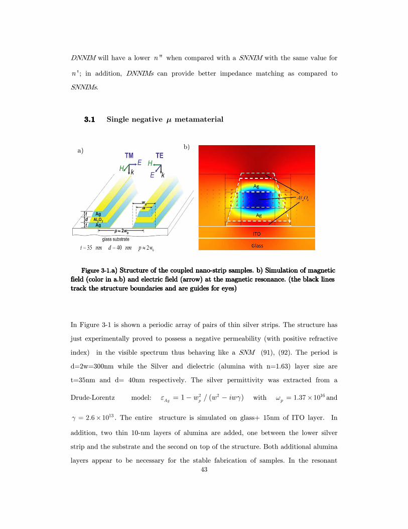
43

DNNIM will have a lower ''n when compared with a SNNIM with the same value for

'n ; in addition, DNNIMs can provide better impedance matching as compared to

SNNIMs.

3.13.13.13.1 Single negative µ metamaterial

Figure Figure Figure Figure 3333----1111....a) a) a) a) Structure of the coupled nanStructure of the coupled nanStructure of the coupled nanStructure of the coupled nanoooo----strip samples.strip samples.strip samples.strip samples. b) Simulation of magnetic b) Simulation of magnetic b) Simulation of magnetic b) Simulation of magnetic

field (color in a.b) and electric field (arrow) at the magnetic resonance. (the black lines field (color in a.b) and electric field (arrow) at the magnetic resonance. (the black lines field (color in a.b) and electric field (arrow) at the magnetic resonance. (the black lines field (color in a.b) and electric field (arrow) at the magnetic resonance. (the black lines

track the structure boundaries and are guides for eyes)track the structure boundaries and are guides for eyes)track the structure boundaries and are guides for eyes)track the structure boundaries and are guides for eyes)

In Figure 3-1 is shown a periodic array of pairs of thin silver strips. The structure has

just experimentally proved to possess a negative permeability (with positive refractive

index) in the visible spectrum thus behaving like a SNM (91), (92). The period is

d=2w=300nm while the Silver and dielectric (alumina with n=1.63) layer size are

t=35nm and d= 40nm respectively. The silver permittivity was extracted from a

Drude-Lorentz model: 2 21 / ( )Ag p

w w iwε γ= − − with 161.37 10pω = × and

132.6 10γ = × . The entire structure is simulated on glass+ 15nm of ITO layer. In

addition, two thin 10-nm layers of alumina are added, one between the lower silver

strip and the substrate and the second on top of the structure. Both additional alumina

layers appear to be necessary for the stable fabrication of samples. In the resonant

a)

b)

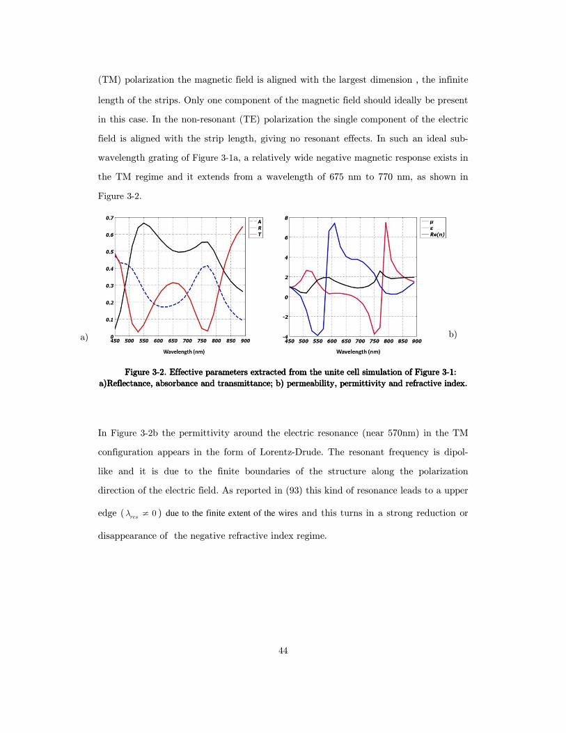
44

(TM) polarization the magnetic field is aligned with the largest dimension , the infinite

length of the strips. Only one component of the magnetic field should ideally be present

in this case. In the non-resonant (TE) polarization the single component of the electric

field is aligned with the strip length, giving no resonant effects. In such an ideal sub-

wavelength grating of Figure 3-1a, a relatively wide negative magnetic response exists in

the TM regime and it extends from a wavelength of 675 nm to 770 nm, as shown in

Figure 3-2.

Figure Figure Figure Figure 3333----2222. Effective parameters extracted from the unite cell simulation of . Effective parameters extracted from the unite cell simulation of . Effective parameters extracted from the unite cell simulation of . Effective parameters extracted from the unite cell simulation of Figure Figure Figure Figure 3333----1111::::

a)Reflectanca)Reflectanca)Reflectanca)Reflectance, absorbance and transmie, absorbance and transmie, absorbance and transmie, absorbance and transmittttttttance;ance;ance;ance; b) permeability, permittivity and refractive indexb) permeability, permittivity and refractive indexb) permeability, permittivity and refractive indexb) permeability, permittivity and refractive index....

In Figure 3-2b the permittivity around the electric resonance (near 570nm) in the TM

configuration appears in the form of Lorentz-Drude. The resonant frequency is dipol-

like and it is due to the finite boundaries of the structure along the polarization

direction of the electric field. As reported in (93) this kind of resonance leads to a upper

edge ( 0resλ ≠ ) due to the finite extent of the wires and this turns in a strong reduction or

disappearance of the negative refractive index regime.

a) b)

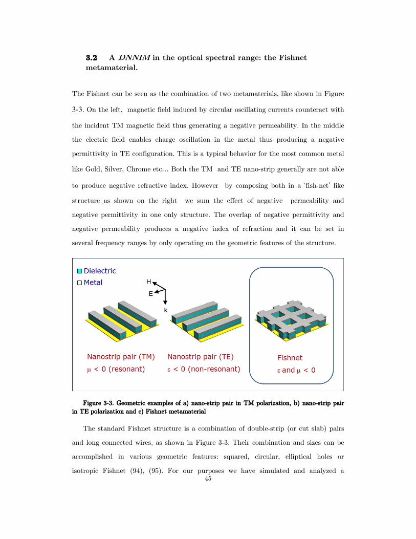
45

3.23.23.23.2 A DNNIM in the optical spectral range: the Fishnet

metamaterial.

The Fishnet can be seen as the combination of two metamaterials, like shown in Figure

3-3. On the left, magnetic field induced by circular oscillating currents counteract with

the incident TM magnetic field thus generating a negative permeability. In the middle

the electric field enables charge oscillation in the metal thus producing a negative

permittivity in TE configuration. This is a typical behavior for the most common metal

like Gold, Silver, Chrome etc… Both the TM and TE nano-strip generally are not able

to produce negative refractive index. However by composing both in a ‘fish-net’ like

structure as shown on the right we sum the effect of negative permeability and

negative permittivity in one only structure. The overlap of negative permittivity and

negative permeability produces a negative index of refraction and it can be set in

several frequency ranges by only operating on the geometric features of the structure.

Figure Figure Figure Figure 3333----3333. Geometric examples of a) nano. Geometric examples of a) nano. Geometric examples of a) nano. Geometric examples of a) nano----strip pair in TM polarization, b) nanostrip pair in TM polarization, b) nanostrip pair in TM polarization, b) nanostrip pair in TM polarization, b) nano----strip pair strip pair strip pair strip pair

in TE polarization and c) in TE polarization and c) in TE polarization and c) in TE polarization and c) FishnetFishnetFishnetFishnet metamaterialmetamaterialmetamaterialmetamaterial

The standard Fishnet structure is a combination of double-strip (or cut slab) pairs

and long connected wires, as shown in Figure 3-3. Their combination and sizes can be

accomplished in various geometric features: squared, circular, elliptical holes or

isotropic Fishnet (94), (95). For our purposes we have simulated and analyzed a

46

Fishnet with squared holes. The structure is illuminated at normal incident with the

long wires along the electric fields. All the geometric features are illustrated in Figure

3-4. The thickness of the metal (Au) layers and the dielectric (Al2O3) layer are fixed to

t=30 nm and h=40 nm respectively and az=2t+h is the total Fishnet thickness in the

longitudinal (parallel to kkkk) direction. We chose D=150 nm and W= 120 nm as the

major and minor size of the squared holes respectively and P=300 nm is the lattice

parameter in the lateral directions. Alumina (Al2O3) with index of refraction n=1.63

has been chosen for its low losses in the terahertz range. For the extraction of the S-

Parameters and the verification of our design, parametric simulations were done with

the commercial Comsol Multiphysics ® software, employing the Finite Element Method

(FEM) for finding approximate solutions of Maxwell’s equations. The Fishnet has been

regarded theoretically as an artificial waveguide surrounded by air, with two perfect

magnetic conductor planes normal to the incident magnetic fields and two perfect

electric conductor planes normal to the incident electric fields. Two ports under and

above the unite cell Fishnet have been added for the evaluation of the S-Parameters of

the wave-guide. In this way the structure is equivalent to a periodic infinite tri-layer

medium (homogeneous for the operative wavelengths over 400 nm) with a polarized

normal incident wave. Drude model extracted from experimental data for metallic bulk

has been used to describe the electron plasma behavior at the surface of Gold (96),

(97).The value of plasma frequency (ω p ) and collision frequency (γ ) are 2175 THz and

6.5 THz respectively. These values are guaranteed to fit the experimental data over a

frequency range from 30 to 900 THz (96),(97). The effective parameters, permittivity,

permeability and refraction index are retrieved according to the traditional method

(81),(82) by inverting the simulated S-Parameters, under the assumption that the

metamaterial can be treated as homogenous. For most of the potential applications of

metamaterials, like super-lensing resolution, waves propagate at non zero angle of

incidence with respect to the plane perpendicular to the boundary of the structure (EEEE-kkkk

plane). So we recalculated the transmission data of our Fishnet for different angles of

incidence in TE configuration (only a part of the magnetic incident field is oriented

47

parallel to the z-axis) and using circular holes of ray r=76nm. In Figure 3-4 we see that

the spectral position and shape of the observed transmission band in the magnetic

resonant regime varies slightly with the angle of incidence although the magnetic

coupling decrease with larger angles of incidence ( °> 40ϑ ).

Figure Figure Figure Figure 3333----4444. Unit cell of the . Unit cell of the . Unit cell of the . Unit cell of the FishnetFishnetFishnetFishnet with parameters indicated: The lattice constant along xwith parameters indicated: The lattice constant along xwith parameters indicated: The lattice constant along xwith parameters indicated: The lattice constant along x----

y direction P=300 nm, the metal (Au) thickness t=30 nm, the dielectric (Aly direction P=300 nm, the metal (Au) thickness t=30 nm, the dielectric (Aly direction P=300 nm, the metal (Au) thickness t=30 nm, the dielectric (Aly direction P=300 nm, the metal (Au) thickness t=30 nm, the dielectric (Al2222OOOO3333) thickness h=40 ) thickness h=40 ) thickness h=40 ) thickness h=40

nm and the widths of the rectangular holes respectively D=75 nm and W=60 nm. The nm and the widths of the rectangular holes respectively D=75 nm and W=60 nm. The nm and the widths of the rectangular holes respectively D=75 nm and W=60 nm. The nm and the widths of the rectangular holes respectively D=75 nm and W=60 nm. The

electromagnetic field is incident along the z direction, with the electric and magnetic fields in electromagnetic field is incident along the z direction, with the electric and magnetic fields in electromagnetic field is incident along the z direction, with the electric and magnetic fields in electromagnetic field is incident along the z direction, with the electric and magnetic fields in

the x and y direction respectively. the x and y direction respectively. the x and y direction respectively. the x and y direction respectively.

3.33.33.33.3 The effective Fishnet parameters

In Figure 3-5 we show the effective parameters extracted from the simulation. Two

dips in the reflectance (and two corresponding maxima in the transmittance) spectrum

are clearly visible. They are evident manifestation of two resonances at 600nm and

830nm. The two dips in the reflectance correspond to the two local minima of

permeability: µ=-0.46 at 599 nm and µ=-1.52 at 834 nm. Two left handed LH bands

of negative index are foreseen in the two regions: from 595nm to 600nm and from

810nm to 840nm where the real part of permeability and permittivity overlaps giving

rise to a negative refractive index.

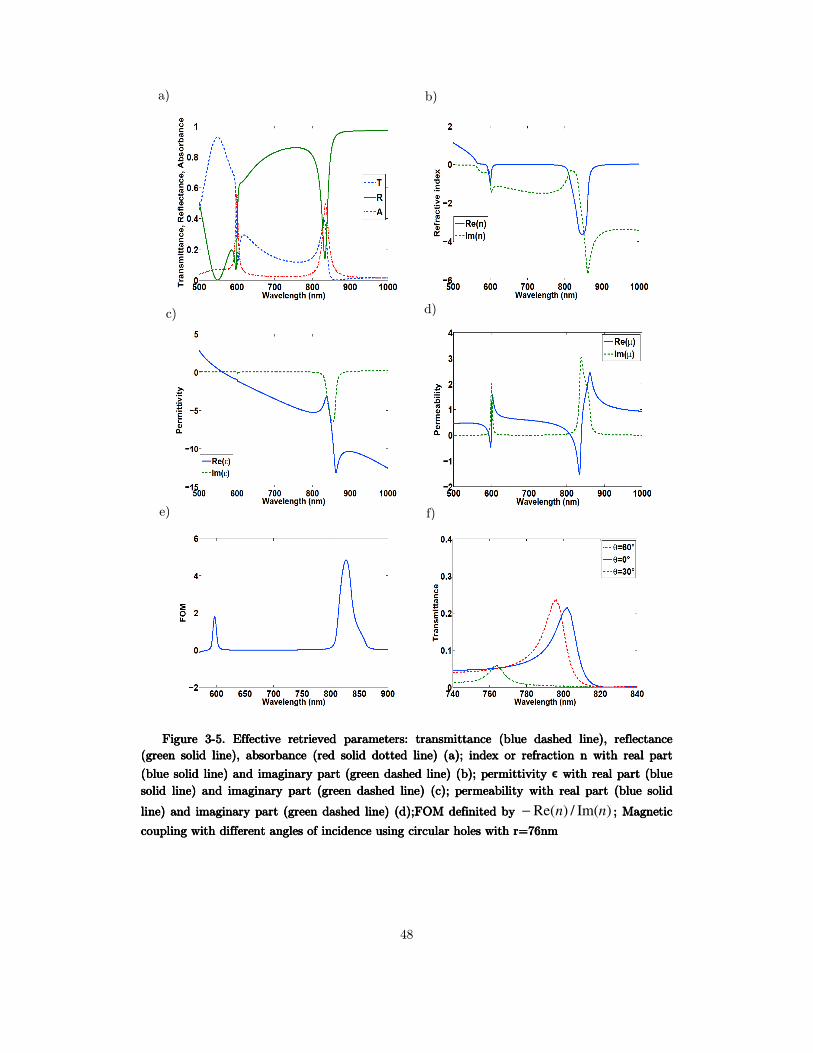
48

Figure Figure Figure Figure 3333----5555. Effective retrieved parameters: transmittance (blue dashed line), reflectance . Effective retrieved parameters: transmittance (blue dashed line), reflectance . Effective retrieved parameters: transmittance (blue dashed line), reflectance . Effective retrieved parameters: transmittance (blue dashed line), reflectance

(green solid line), absorbance (red solid dotted line) (a); index or refraction n with real part (green solid line), absorbance (red solid dotted line) (a); index or refraction n with real part (green solid line), absorbance (red solid dotted line) (a); index or refraction n with real part (green solid line), absorbance (red solid dotted line) (a); index or refraction n with real part

(blue solid line) and imaginary part (green dashed line) (b); permittivity (blue solid line) and imaginary part (green dashed line) (b); permittivity (blue solid line) and imaginary part (green dashed line) (b); permittivity (blue solid line) and imaginary part (green dashed line) (b); permittivity ϵ wiwiwiwith real part (blue th real part (blue th real part (blue th real part (blue

solid line) and imaginary part (green dashed line) (c); permeability with real part (blue solid solid line) and imaginary part (green dashed line) (c); permeability with real part (blue solid solid line) and imaginary part (green dashed line) (c); permeability with real part (blue solid solid line) and imaginary part (green dashed line) (c); permeability with real part (blue solid

line) and imaginary part (green dashed line) (d);FOM definited by line) and imaginary part (green dashed line) (d);FOM definited by line) and imaginary part (green dashed line) (d);FOM definited by line) and imaginary part (green dashed line) (d);FOM definited by )Im(/)Re( nn− ; Magnetic ; Magnetic ; Magnetic ; Magnetic

coupling with different angles of incidenccoupling with different angles of incidenccoupling with different angles of incidenccoupling with different angles of incidence using circular holes with r=76nme using circular holes with r=76nme using circular holes with r=76nme using circular holes with r=76nm

a) b)

c) d)

e) f)

49

3.43.43.43.4 The Fishnet modes (an overview)

The nature of this resonances is quite different. Christ et al (98) and more recently

J.Parson at al (99), have investigated the nature of these modes. They are related to

the hybridization of LSPRs (Localized Surface Plasmon Resonance). The absorbance

maxima in the hole-array structure is attribute to the coupling of the incident radiation

to LRSP modes associated with the charge distribution induced in the vicinity of the

nano-holes. As long as the dielectric separation is not too large (about few tens of

nanometers), we expect two modes to be possible: an electric symmetric and a magnetic

anti-symmetric mode. Symmetric and anti-symmetric refers to the orientation of

currents along the two metal-dielectric interfaces. In Figure 3-6 we show simulations

mapping the electric and the magnetic fields in the unit cell around the hole. In Figure

3-6b two opposite currents are visible inside the hole volume at frequency of 834nm.

a) b)

x

z

50

Figure Figure Figure Figure 3333----6666 MMMMapapapapssss of electric and magnetic fields: Electric field of electric and magnetic fields: Electric field of electric and magnetic fields: Electric field of electric and magnetic fields: Electric field components components components components at at at at the the the the electricelectricelectricelectric

resonanceresonanceresonanceresonance and the z component (contour plot) (a); electric field components (arrows) at and the z component (contour plot) (a); electric field components (arrows) at and the z component (contour plot) (a); electric field components (arrows) at and the z component (contour plot) (a); electric field components (arrows) at

magneticmagneticmagneticmagnetic resonance and the z component (contour plot) (b);resonance and the z component (contour plot) (b);resonance and the z component (contour plot) (b);resonance and the z component (contour plot) (b); magnetic field components at thmagnetic field components at thmagnetic field components at thmagnetic field components at the e e e

magnetic resonance (arrows) and tmagnetic resonance (arrows) and tmagnetic resonance (arrows) and tmagnetic resonance (arrows) and the y component (contour plot) (he y component (contour plot) (he y component (contour plot) (he y component (contour plot) (cccc); For the 3 cases the unit ); For the 3 cases the unit ); For the 3 cases the unit ); For the 3 cases the unit

cell has been centered around the hole and the observation planes have been fixed at P/2 in the cell has been centered around the hole and the observation planes have been fixed at P/2 in the cell has been centered around the hole and the observation planes have been fixed at P/2 in the cell has been centered around the hole and the observation planes have been fixed at P/2 in the

y direction (a,by direction (a,by direction (a,by direction (a,b) and az/2 in the z direction () and az/2 in the z direction () and az/2 in the z direction () and az/2 in the z direction (cccc) respectively.) respectively.) respectively.) respectively.

The π-phase change in the incident electric field is not possible over a distance less

than one wavelength (which in turn enforces the homogeneity condition). Instead, the

excitation of the anti-ymmetric mode occurs through the incident time-varying

magnetic field which induces currents in both the upper and lower layers being in anti-

phase. For this reason this kind of resonance is referred to as a magnetic resonance. In

Figure 3-6b is also shown the z-component of the electric fields. Two effective magnetic

capacitance are generated by the magnetic resonance as it appears from the arrows of

the electric field in the z-direction. In Figure 3-6c are also shown the magnetic fields

components (arrow plot). The magnetic field components at the resonance have

opposed direction between the neck and the slab. This is consequence of counteracting

currents between the neck and the slab generated by opposite charges between the

slabs (see the arrows in opposite directions between the neck and the slab). This

produces two magnetic inductances in parallel. As a result a resonant magnetic LC

circuit is induced by the charge distribution in the Fishnet metamaterial. Moreover

from Figure 3-6a the current distribution around the hole appears symmetric at

frequency of 598nm and its related resonance is mainly electric in nature. In this case

the currents flow through the electric capacitance between two parallel wires of

approximate length P and radius t without charge accumulation between the slab and

c)

x

y

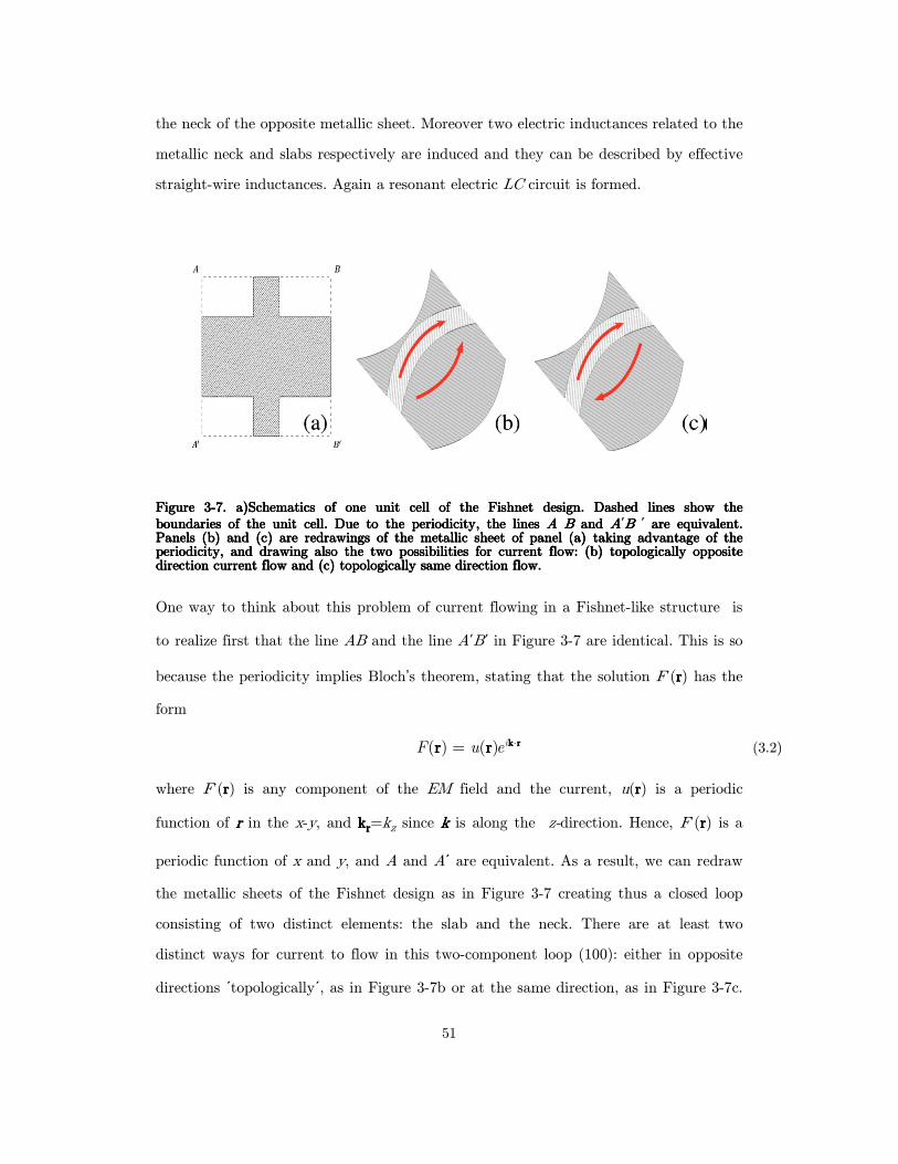
51

the neck of the opposite metallic sheet. Moreover two electric inductances related to the

metallic neck and slabs respectively are induced and they can be described by effective

straight-wire inductances. Again a resonant electric LC circuit is formed.

Figure Figure Figure Figure 3333----7777.... aaaa))))Schematics of oneSchematics of oneSchematics of oneSchematics of one unit cell of the unit cell of the unit cell of the unit cell of the FishnetFishnetFishnetFishnet design. Dashed lines show tdesign. Dashed lines show tdesign. Dashed lines show tdesign. Dashed lines show the he he he boundaries of the unit cell. boundaries of the unit cell. boundaries of the unit cell. boundaries of the unit cell. Due to the periodicity, the lines Due to the periodicity, the lines Due to the periodicity, the lines Due to the periodicity, the lines AAAA B B B B and and and and AAAA΄BBBB ΄ are equivalent. are equivalent. are equivalent. are equivalent. Panels (Panels (Panels (Panels (bbbb)))) and and and and ((((cccc)))) are redrawings of the metallic sheet of panel are redrawings of the metallic sheet of panel are redrawings of the metallic sheet of panel are redrawings of the metallic sheet of panel ((((aaaa)))) taking taking taking taking advantage of the advantage of the advantage of the advantage of the periodicity, and draperiodicity, and draperiodicity, and draperiodicity, and drawing also the two possibilities wing also the two possibilities wing also the two possibilities wing also the two possibilities for current flow: for current flow: for current flow: for current flow: ((((bbbb)))) topologically topologically topologically topologically opposite opposite opposite opposite direction current flow direction current flow direction current flow direction current flow and and and and ((((cccc)))) topologically same direction flowtopologically same direction flowtopologically same direction flowtopologically same direction flow.... One way to think about this problem of current flowing in a Fishnet-like structure is

to realize first that the line AB and the line A΄B΄ in Figure 3-7 are identical. This is so

because the periodicity implies Bloch’s theorem, stating that the solution F˙(rrrr) has the

form

( ) ( ) iF u e ⋅= k rk rk rk rr rr rr rr r (3.2)

where F˙(rrrr) is any component of the EM field and the current, u(rrrr) is a periodic

function of rrrr in the x-y, and kkkkrrrr=kz since kkkk is along the z-direction. Hence, F˙(rrrr) is a

periodic function of x and y, and A and A΄ are equivalent. As a result, we can redraw

the metallic sheets of the Fishnet design as in Figure 3-7 creating thus a closed loop

consisting of two distinct elements: the slab and the neck. There are at least two

distinct ways for current to flow in this two-component loop (100): either in opposite

directions ΄topologically΄, as in Figure 3-7b or at the same direction, as in Figure 3-7c.

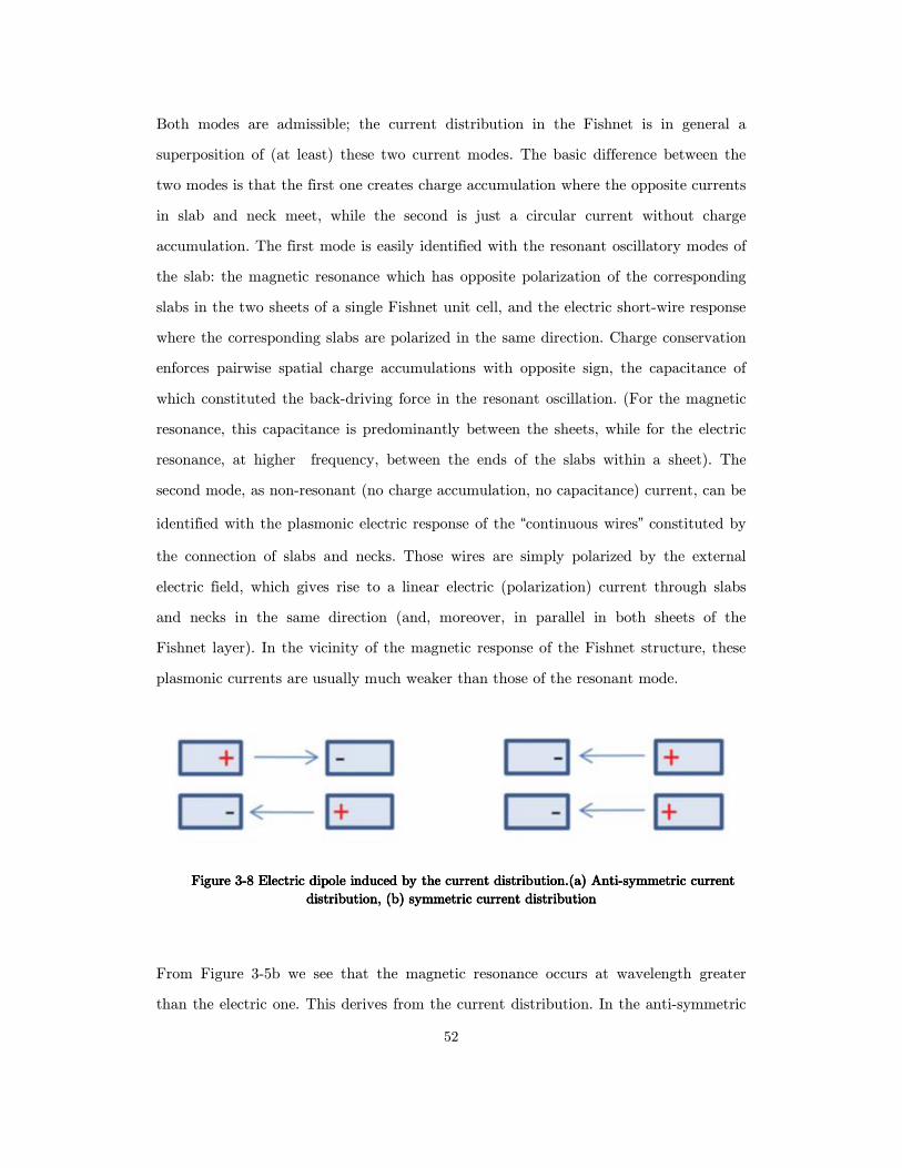
52

Both modes are admissible; the current distribution in the Fishnet is in general a

superposition of (at least) these two current modes. The basic difference between the

two modes is that the first one creates charge accumulation where the opposite currents

in slab and neck meet, while the second is just a circular current without charge

accumulation. The first mode is easily identified with the resonant oscillatory modes of

the slab: the magnetic resonance which has opposite polarization of the corresponding

slabs in the two sheets of a single Fishnet unit cell, and the electric short-wire response

where the corresponding slabs are polarized in the same direction. Charge conservation

enforces pairwise spatial charge accumulations with opposite sign, the capacitance of

which constituted the back-driving force in the resonant oscillation. (For the magnetic

resonance, this capacitance is predominantly between the sheets, while for the electric

resonance, at higher frequency, between the ends of the slabs within a sheet). The

second mode, as non-resonant (no charge accumulation, no capacitance) current, can be

identified with the plasmonic electric response of the “continuous wires” constituted by

the connection of slabs and necks. Those wires are simply polarized by the external

electric field, which gives rise to a linear electric (polarization) current through slabs

and necks in the same direction (and, moreover, in parallel in both sheets of the

Fishnet layer). In the vicinity of the magnetic response of the Fishnet structure, these

plasmonic currents are usually much weaker than those of the resonant mode.

Figure Figure Figure Figure 3333----8888 Electric dipole induced by the current distribution.(a) AntiElectric dipole induced by the current distribution.(a) AntiElectric dipole induced by the current distribution.(a) AntiElectric dipole induced by the current distribution.(a) Anti----symmetric current symmetric current symmetric current symmetric current

distribution, (b) symmetric current distributiondistribution, (b) symmetric current distributiondistribution, (b) symmetric current distributiondistribution, (b) symmetric current distribution

From Figure 3-5b we see that the magnetic resonance occurs at wavelength greater

than the electric one. This derives from the current distribution. In the anti-symmetric

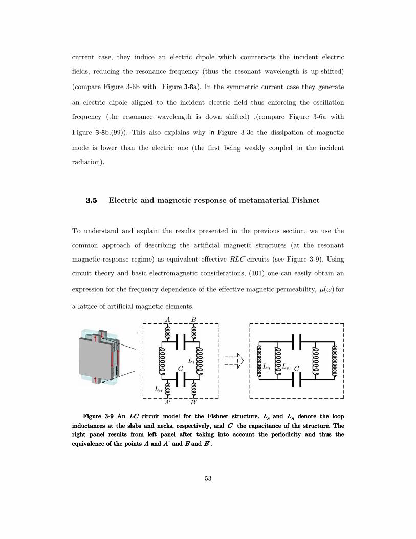
53

current case, they induce an electric dipole which counteracts the incident electric

fields, reducing the resonance frequency (thus the resonant wavelength is up-shifted)

(compare Figure 3-6b with Figure 3-8a). In the symmetric current case they generate

an electric dipole aligned to the incident electric field thus enforcing the oscillation

frequency (the resonance wavelength is down shifted) ,(compare Figure 3-6a with

Figure 3-8b,(99)). This also explains why in Figure 3-3e the dissipation of magnetic

mode is lower than the electric one (the first being weakly coupled to the incident

radiation).

3.53.53.53.5 Electric and magnetic response of metamaterial Fishnet

To understand and explain the results presented in the previous section, we use the

common approach of describing the artificial magnetic structures (at the resonant

magnetic response regime) as equivalent effective RLC circuits (see Figure 3-9). Using

circuit theory and basic electromagnetic considerations, (101) one can easily obtain an

expression for the frequency dependence of the effective magnetic permeability, ( )µ ω for

a lattice of artificial magnetic elements.

Figure Figure Figure Figure 3333----9999 An An An An LC LC LC LC circuit model for the circuit model for the circuit model for the circuit model for the FishnetFishnetFishnetFishnet structure. structure. structure. structure. LLLLssss and and and and LLLLnnnn denote the loop denote the loop denote the loop denote the loop

inductances at the slabs and necks, respectively, andinductances at the slabs and necks, respectively, andinductances at the slabs and necks, respectively, andinductances at the slabs and necks, respectively, and CCCC the capacitance of the structure. The the capacitance of the structure. The the capacitance of the structure. The the capacitance of the structure. The

right panel results from leftright panel results from leftright panel results from leftright panel results from left panel after taking into account the periodicity and thus the panel after taking into account the periodicity and thus the panel after taking into account the periodicity and thus the panel after taking into account the periodicity and thus the

equivalenceequivalenceequivalenceequivalence of the points of the points of the points of the points A A A A and and and and AAAA΄ and and and and B B B B and and and and BBBB΄....

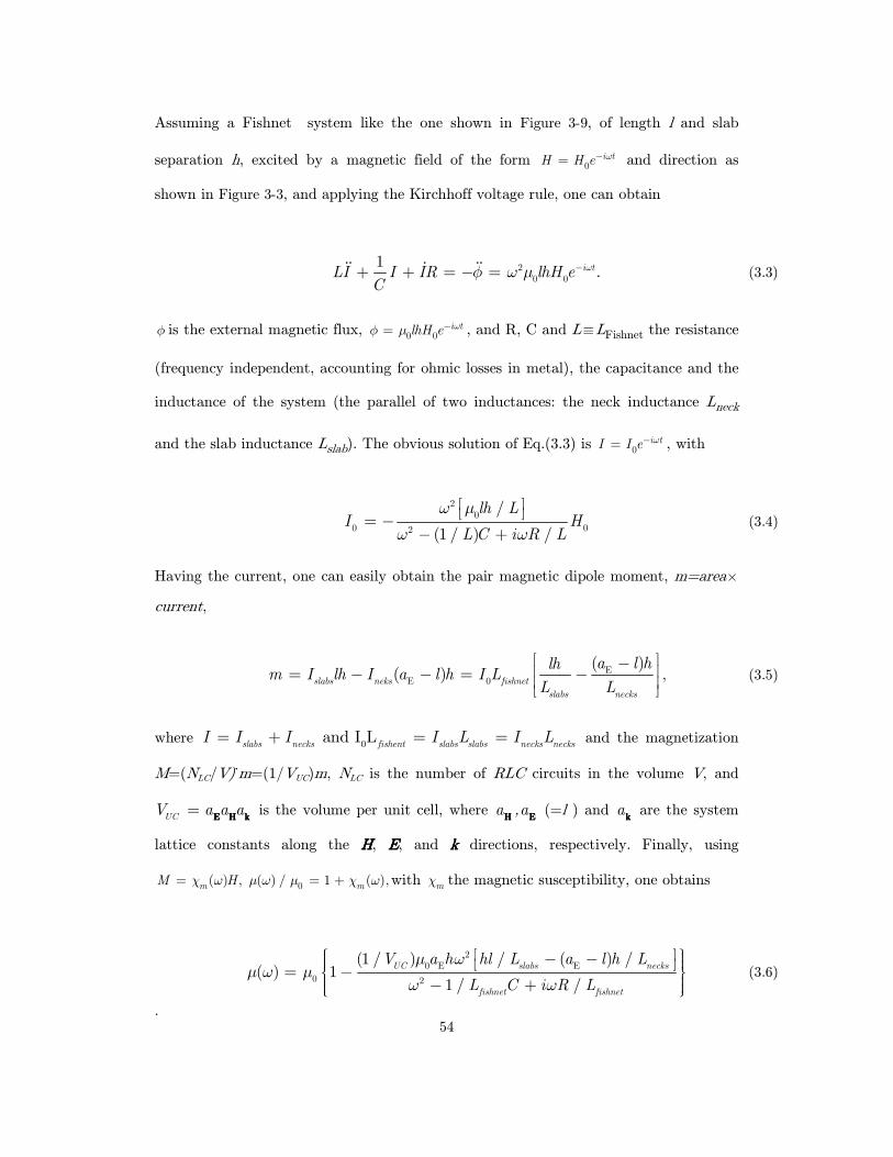
54

Assuming a Fishnet system like the one shown in Figure 3-9, of length l and slab

separation h, excited by a magnetic field of the form 0i tH H e ω−= and direction as

shown in Figure 3-3, and applying the Kirchhoff voltage rule, one can obtain

20 0

1.i tLI I IR lhH e

C

ωφ ω µ −+ + = − =ɺɺ ɺ ɺɺ (3.3)

φ is the external magnetic flux, 0 0i tlhH e ωφ µ −= , and R, C and L≡LFishnet the resistance

(frequency independent, accounting for ohmic losses in metal), the capacitance and the

inductance of the system (the parallel of two inductances: the neck inductance Lneck

and the slab inductance Lslab). The obvious solution of Eq.(3.3) is 0i tI I e ω−= , with

20

0 02

/

(1 / ) /

lh LI H

L C i R L

ω µ

ω ω

= −

− + (3.4)

Having the current, one can easily obtain the pair magnetic dipole moment, m=area×

current,

EE 0

( )( )

slabs neks fishnet

slabs necks

a l hlhm I lh I a l h I L

L L

− = − − = −

, (3.5)

where 0 and I L

slabs necks fishent slabs slabs necks necksI I I I L I L= + = = and the magnetization

M=(NLC/V)˙m=(1/VUC)m, NLC is the number of RLC circuits in the volume V, and

UCV a a a=

E H kE H kE H kE H k is the volume per unit cell, where a

HHHH,a

EEEE (=l ) and a

kkkk are the system

lattice constants along the HHHH, EEEE, and kkkk directions, respectively. Finally, using

0( ) , ( ) / 1 ( ),m mM Hχ ω µ ω µ χ ω= = + with mχ the magnetic susceptibility, one obtains

20 E E

0 2

(1 / ) / ( ) /( ) 1

1 / /

UC slabs necks

fishnet fishnet

V a h hl L a l h L

L C i R L

µ ωµ ω µ

ω ω

− − = − − +

(3.6)

.

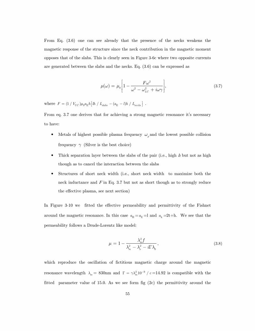
55

From Eq. (3.6) one can see already that the presence of the necks weakens the

magnetic response of the structure since the neck contribution in the magnetic moment

opposes that of the slabs. This is clearly seen in Figure 3-6c where two opposite currents

are generated between the slabs and the necks. Eq. (3.6) can be expressed as

2

0 2 2( ) 1 ,

LC

F

i

ωµ ω µ

ω ω ωγ

= − − +

(3.7)

where 0 E E(1 / ) / ( ) /UC slabs necksF V a h lh L a l h Lµ = − − .

From eq. 3.7 one derives that for achieving a strong magnetic resonance it’s necessary

to have:

• Metals of highest possible plasma frequency pω and the lowest possible collision

frequency γ (Silver is the best choice)

• Thick separation layer between the slabs of the pair (i.e., high h but not as high

though as to cancel the interaction between the slabs

• Structures of short neck width (i.e., short neck width to maximize both the

neck inductance and F in Eq. 3.7 but not as short though as to strongly reduce

the effective plasma, see next section)

In Figure 3-10 we fitted the effective permeability and permittivity of the Fishnet

around the magnetic resonance. In this case Ha = Ea =l and ka =2t+h. We see that the

permeability follows a Drude-Lorentz like model:

2

2 20

1 m

m o

f

i

λµ

λ λ λ= −

− − Γ, (3.8)

which reproduce the oscillation of fictitious magnetic charge around the magnetic

resonance wavelength mλ = 830nm and 2 910 /m cγλ −Γ = =14.92 is compatible with the

fitted parameter value of 15.0. As we see form fig (2c) the permittivity around the

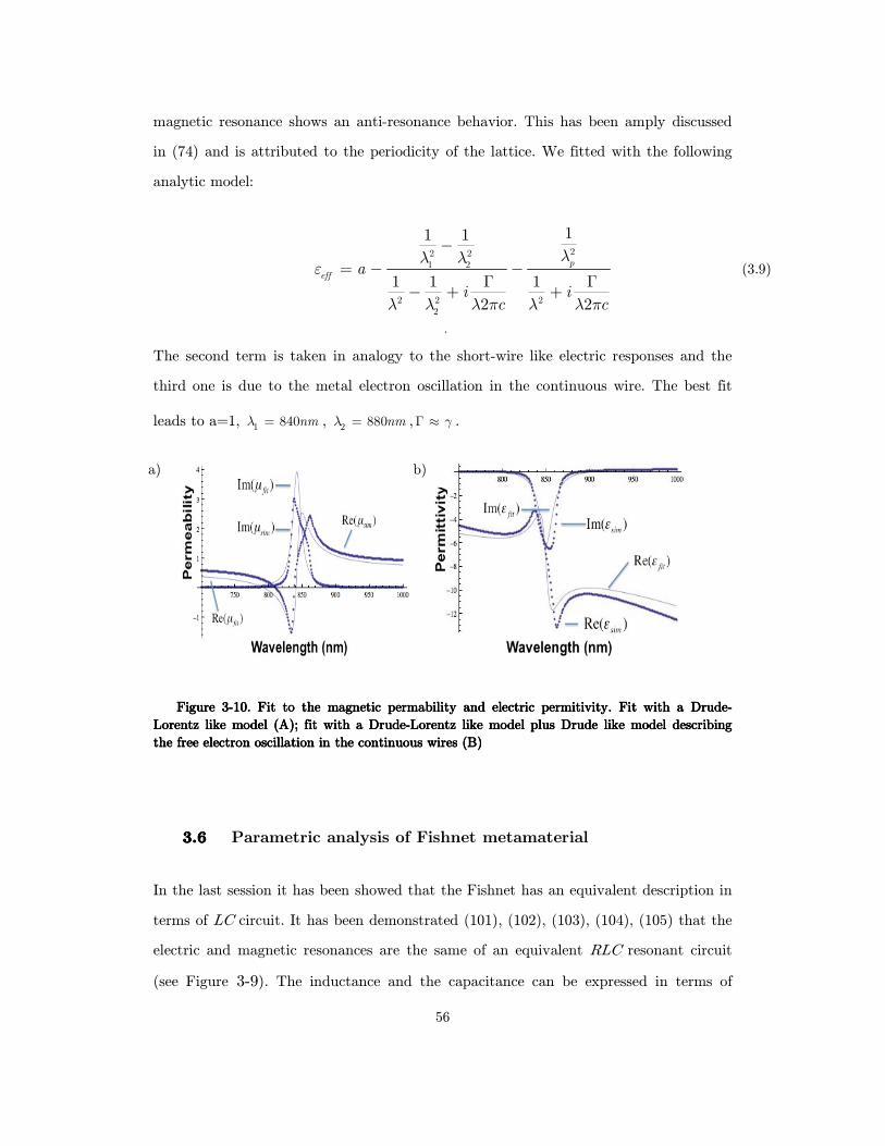
56

magnetic resonance shows an anti-resonance behavior. This has been amply discussed

in (74) and is attributed to the periodicity of the lattice. We fitted with the following

analytic model:

22 21 2

2 2 22

11 1

1 1 1

2 2

p

effa

i ic c

λλ λε

λ π λ πλ λ λ

−

= − −Γ Γ

− + +

(3.9)

.

The second term is taken in analogy to the short-wire like electric responses and the

third one is due to the metal electron oscillation in the continuous wire. The best fit

leads to a=1, 1 840nmλ = , 2 880nmλ = , γΓ ≈ .

Figure Figure Figure Figure 3333----10101010. . . . Fit to the magnetic permability and electric permitivity. Fit with a DrudeFit to the magnetic permability and electric permitivity. Fit with a DrudeFit to the magnetic permability and electric permitivity. Fit with a DrudeFit to the magnetic permability and electric permitivity. Fit with a Drude----

Lorentz like model (A); fit with a DrudeLorentz like model (A); fit with a DrudeLorentz like model (A); fit with a DrudeLorentz like model (A); fit with a Drude----Lorentz like model plus Drude Lorentz like model plus Drude Lorentz like model plus Drude Lorentz like model plus Drude like model describing like model describing like model describing like model describing

the free electron oscillation in the continuous wires (B)the free electron oscillation in the continuous wires (B)the free electron oscillation in the continuous wires (B)the free electron oscillation in the continuous wires (B)

3.63.63.63.6 Parametric analysis of Fishnet metamaterial

In the last session it has been showed that the Fishnet has an equivalent description in

terms of LC circuit. It has been demonstrated (101), (102), (103), (104), (105) that the

electric and magnetic resonances are the same of an equivalent RLC resonant circuit

(see Figure 3-9). The inductance and the capacitance can be expressed in terms of

a) b)

57

geometric parameters. In the case of magnetic mode ,for example, the capacity can be

approximated by that of a capacitance with plate faces and the inductance can be

approximated by that of a solenoid. The inductance for both the magnetic and electric

mode is the parallel with the inductance generated by the slab and that generated by

the necks. With this assumption it’s possible to approximate the magnetic capacitance

and inductance as:

( ) ( ) ( )( ) ( )2 / 2 , 1 / 1 /m mm mslabs necksC P P W h L L L− +≃ ≃ , (3.10)

where ( )( ) 2 /mslabsL P W h P−≃ and ( )( ) / 2m

necksL Wh P D−≃ , see Figure 3-9.

As a result a magnetic LC circuit is induced by the charge distribution in the Fishnet

with magnetic resonance frequency given by (102).

2( ) ( )

1 1 2 ( 2 )

2 ( 2 )( 2 )2m m m

d

c P DK

WP P WP WL Cω

π επ

−= = +

−− (3.11)

Where c is the light speed and dε is the dielectric permittivity constant. On the other

hand because of anti-parallel currents between the slab and the neck at the electric

resonance frequency, the effective neck’s inductance ( )enecksL is in parallel with the slab

inductance ( )eslabsL . As a consequence, the electric resonance frequency is given by (102):

( ) ( )

1 ln( / )

2 22 ( 2 )ln ln2

e e e

c b t A B

P P W WL C P W WP P D

ωππ

= = + − − −

(3.12)

where ( ) / ln( / )eC P b t= is the approximate capacitance between two parallel wires

of length P and radius t, (b is the separation between neighbor short-cut wires, it’s the

same of 2W) and the inductances ( )( ) ( 2 )ln ( 2 ) /e

slabsL P W P W P= − − and

58

( )( ) ln / ( 2 )e

necksL W W P D= − are approximate formulas for a straight-wire

inductance.

In the last relation, the increase of the first term in the sum (as a result of increasing

W) counteracts the decrease of the first one and this leaves the electric resonance

frequency almost unaffected (except the slow logarithmic variation ln(b/t)). The

constant K, A, B are intrinsically related to the shape of the system and they don’t

have a simple analytic expression related to the geometric parameters. From Figure

3-5b it’s possible to see that the electric resonance lies well above the magnetic

resonance frequency mω . Therefore, the effective electric response of the Fishnet design

is actually the Drude-like electric response of the continuous wires only. This effect is

associated with an advantage for the LH behavior of the structure, stemming from the

fact that the Drude-like effective ε experiences slower changes than an effective ε

influenced by electric resonances and this allows a wide frequency spectrum of negative

effective permittivity negative into which the negative permeability can overlap thus

accomplish for negative effective refractive index.

3.73.73.73.7 Parametric simulations under D, W, h variation

The simulations will prove that the LC model is an effective description and guideline

for metamaterial Fishnet. In order to optimize our design we perform a complete

analysis varying all the geometric features of the Fishnet. In Figure 3-11 we perform a

parametric simulation varying the width W of the squared holes. As shown in Figure

3-11, when W decreases both the electric and magnetic resonant wavelength increase

(the electric resonance wavelength increases slowly due to the logarithmic dependence

as just discussed above). This is predicted by the above formulas (Eqs.3.11-3.12).

Physically, when W decreases, the electric-induced slab-dipole resonance wavelength

59

tends to increase (the resonance frequency tends to decrease). Thus the slab dipoles

interact with the incident electric fields leading to a decrease of the resonance

frequency. In Figure 3-11 the resonance at λ=600nm change from LH to RH when W

decreases (the plasma wavelength is up-shifted). Moreover, reducing the parameter W

corresponds to reducing the area of the holes thus disturbing the magnetic performance

of the Fishnet. This leads to a weaker strength and to a positive values for the

permeability around the electric resonance, see Figure 3-11c.

Figure Figure Figure Figure 3333----11111111.... RRRRefractive index (A), permittivity (B), permeability (C) varying the W efractive index (A), permittivity (B), permeability (C) varying the W efractive index (A), permittivity (B), permeability (C) varying the W efractive index (A), permittivity (B), permeability (C) varying the W

parameters of the holes (from 25 to 110 nm).parameters of the holes (from 25 to 110 nm).parameters of the holes (from 25 to 110 nm).parameters of the holes (from 25 to 110 nm).

In Figure 3-12 we perform a parametric analysis of the effective index of the Fishnet

varying the hole width parameter D Figure 3-4. We see that both the magnetic and the

electric resonances wavelengths increase when D increases. This is confirmed by the

a) b)

c)

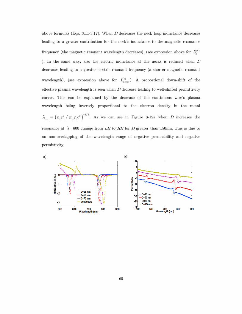
60

above formulas (Eqs. 3.11-3.12). When D decreases the neck loop inductance decreases

leading to a greater contribution for the neck’s inductance to the magnetic resonance

frequency (the magnetic resonant wavelength decreases), (see expression above for ( )mnL

). In the same way, also the electric inductance at the necks is reduced when D

decreases leading to a greater electric resonant frequency (a shorter magnetic resonant

wavelength), (see expression above for ( )enecksL ). A proportional down-shift of the

effective plasma wavelength is seen when D decrease leading to well-shifted permittivity

curves. This can be explained by the decrease of the continuous wire’s plasma

wavelength being inversely proportional to the electron density in the metal

( )1/2

2 2, 0

/e p e

n e m cε

λ ε−

= . As we can see in Figure 3-12a when D increases the

resonance at λ=600 change from LH to RH for D greater than 150nm. This is due to

an non-overlapping of the wavelength range of negative permeability and negative

permittivity.

a) b)

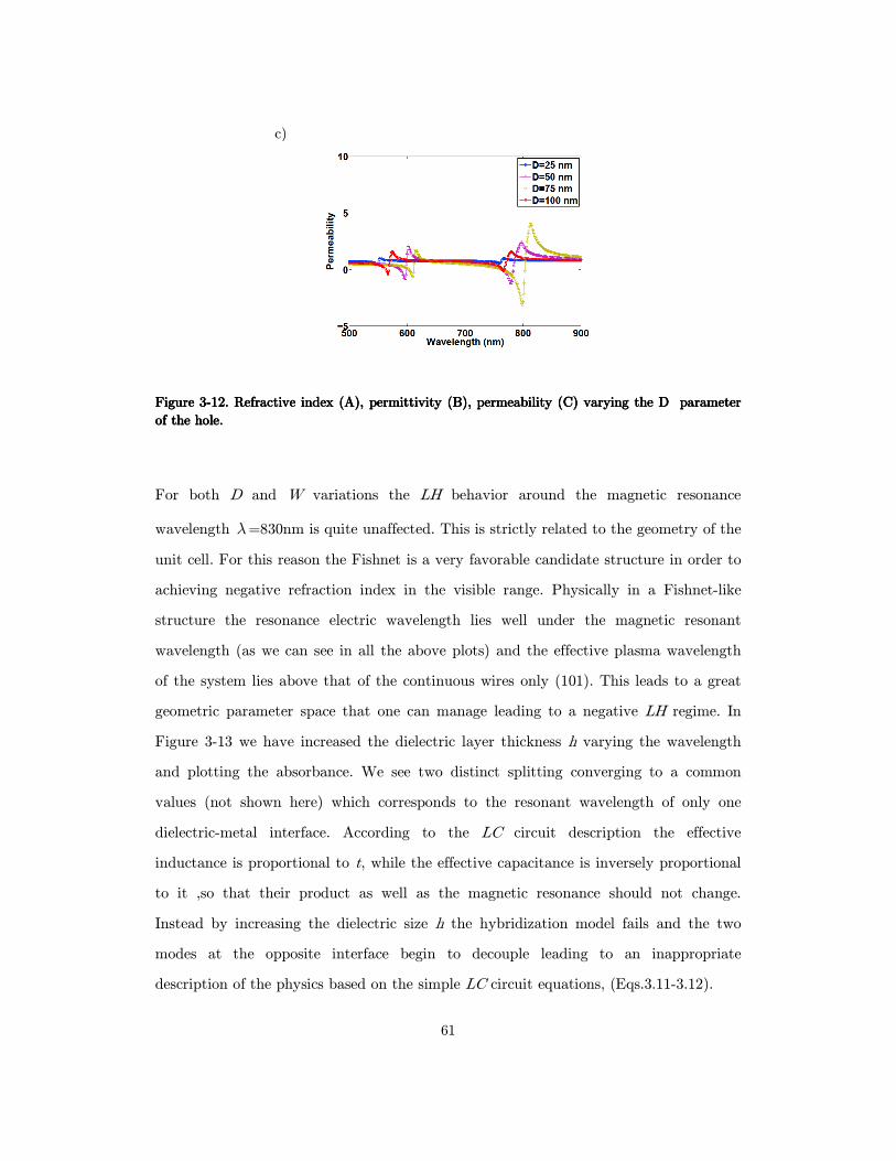
61

Figure Figure Figure Figure 3333----12121212. Refractive index (A), permittivity (B), permeability (C) varying the D parameter . Refractive index (A), permittivity (B), permeability (C) varying the D parameter . Refractive index (A), permittivity (B), permeability (C) varying the D parameter . Refractive index (A), permittivity (B), permeability (C) varying the D parameter

of the hole.of the hole.of the hole.of the hole.

For both D and W variations the LH behavior around the magnetic resonance

wavelength λ=830nm is quite unaffected. This is strictly related to the geometry of the

unit cell. For this reason the Fishnet is a very favorable candidate structure in order to

achieving negative refraction index in the visible range. Physically in a Fishnet-like

structure the resonance electric wavelength lies well under the magnetic resonant

wavelength (as we can see in all the above plots) and the effective plasma wavelength

of the system lies above that of the continuous wires only (101). This leads to a great

geometric parameter space that one can manage leading to a negative LH regime. In

Figure 3-13 we have increased the dielectric layer thickness h varying the wavelength

and plotting the absorbance. We see two distinct splitting converging to a common

values (not shown here) which corresponds to the resonant wavelength of only one

dielectric-metal interface. According to the LC circuit description the effective

inductance is proportional to t, while the effective capacitance is inversely proportional

to it ,so that their product as well as the magnetic resonance should not change.

Instead by increasing the dielectric size h the hybridization model fails and the two

modes at the opposite interface begin to decouple leading to an inappropriate

description of the physics based on the simple LC circuit equations, (Eqs.3.11-3.12).

c)

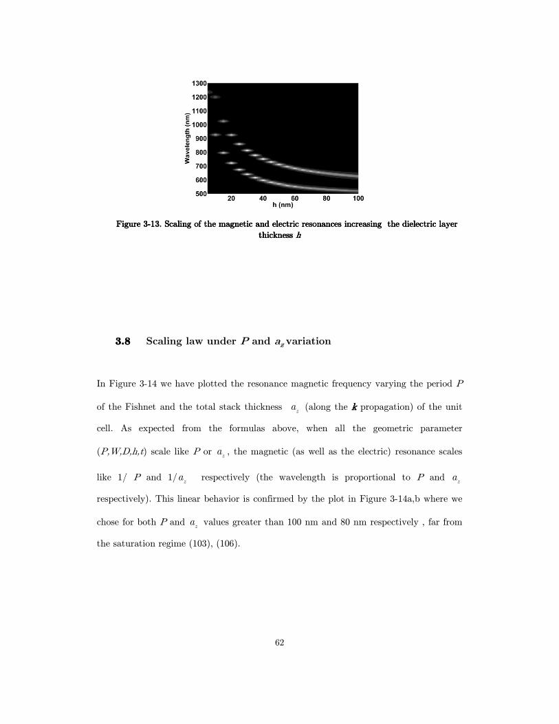
62

Figure Figure Figure Figure 3333----13131313. . . . Scaling of the magnetic and electric resonances increasing the dielectric layer Scaling of the magnetic and electric resonances increasing the dielectric layer Scaling of the magnetic and electric resonances increasing the dielectric layer Scaling of the magnetic and electric resonances increasing the dielectric layer

thicknessthicknessthicknessthickness hhhh

3.83.83.83.8 Scaling law under P and az variation

In Figure 3-14 we have plotted the resonance magnetic frequency varying the period P

of the Fishnet and the total stack thickness za (along the kkkk propagation) of the unit

cell. As expected from the formulas above, when all the geometric parameter

(P,W,D,h,t) scale like P or za , the magnetic (as well as the electric) resonance scales

like 1/ P and 1/za respectively (the wavelength is proportional to P and

za

respectively). This linear behavior is confirmed by the plot in Figure 3-14a,b where we

chose for both P and za values greater than 100 nm and 80 nm respectively , far from

the saturation regime (103), (106).

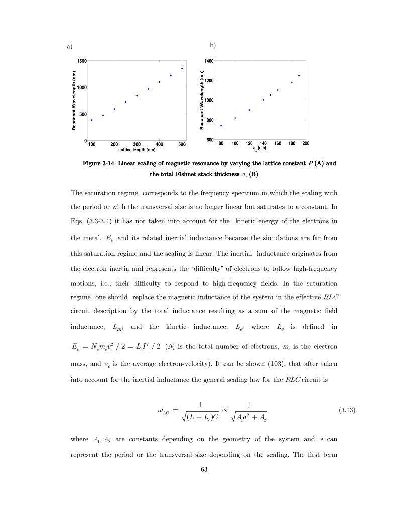
63

Figure Figure Figure Figure 3333----14141414.... Linear scaling of magnetic resonance by varying the lattice constant Linear scaling of magnetic resonance by varying the lattice constant Linear scaling of magnetic resonance by varying the lattice constant Linear scaling of magnetic resonance by varying the lattice constant PPPP (A) and (A) and (A) and (A) and

the total the total the total the total FishnetFishnetFishnetFishnet stack thickness stack thickness stack thickness stack thickness za (B)(B)(B)(B)

The saturation regime corresponds to the frequency spectrum in which the scaling with

the period or with the transversal size is no longer linear but saturates to a constant. In

Eqs. (3.3-3.4) it has not taken into account for the kinetic energy of the electrons in

the metal, k

E and its related inertial inductance because the simulations are far from

this saturation regime and the scaling is linear. The inertial inductance originates from

the electron inertia and represents the “difficulty” of electrons to follow high-frequency

motions, i.e., their difficulty to respond to high-frequency fields. In the saturation

regime one should replace the magnetic inductance of the system in the effective RLC

circuit description by the total inductance resulting as a sum of the magnetic field

inductance, Lm, and the kinetic inductance, Le, where Le is defined in

2 2/ 2 / 2k e e e e

E N m v L I= = (Ne is the total number of electrons, me is the electron

mass, and ve is the average electron-velocity). It can be shown (103), that after taken

into account for the inertial inductance the general scaling law for the RLC circuit is

2

1 2

1 1

( )LC

eL L C Aa A

ω = ∝+ +

(3.13)

where 1A , 2A are constants depending on the geometry of the system and a can

represent the period or the transversal size depending on the scaling. The first term

a) b)

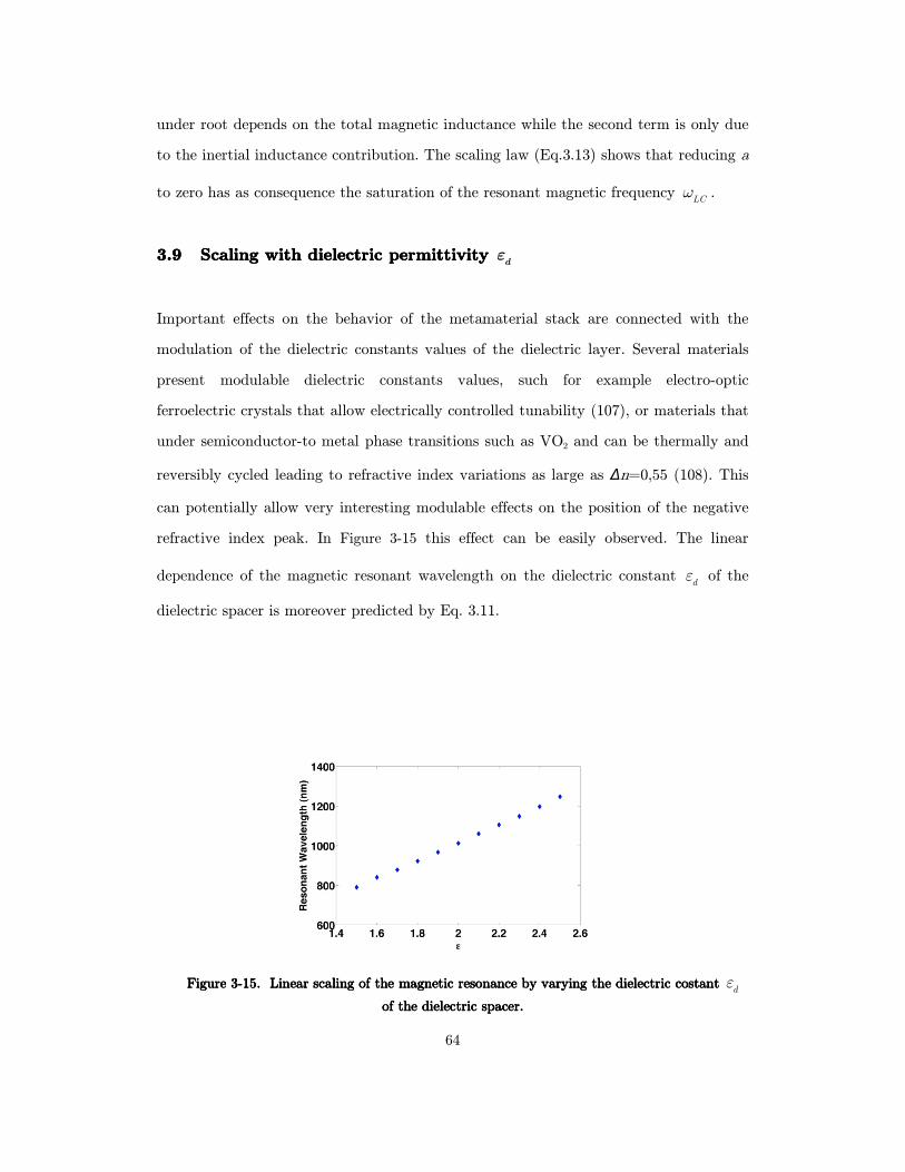
64

under root depends on the total magnetic inductance while the second term is only due

to the inertial inductance contribution. The scaling law (Eq.3.13) shows that reducing a

to zero has as consequence the saturation of the resonant magnetic frequency LCω .

3.93.93.93.9 Scaling with dielectric permittivity Scaling with dielectric permittivity Scaling with dielectric permittivity Scaling with dielectric permittivity dε

Important effects on the behavior of the metamaterial stack are connected with the

modulation of the dielectric constants values of the dielectric layer. Several materials

present modulable dielectric constants values, such for example electro-optic

ferroelectric crystals that allow electrically controlled tunability (107), or materials that

under semiconductor-to metal phase transitions such as VO2 and can be thermally and

reversibly cycled leading to refractive index variations as large as ∆n=0,55 (108). This

can potentially allow very interesting modulable effects on the position of the negative

refractive index peak. In Figure 3-15 this effect can be easily observed. The linear

dependence of the magnetic resonant wavelength on the dielectric constant dε of the

dielectric spacer is moreover predicted by Eq. 3.11.

Figure Figure Figure Figure 3333----15151515. . . . Linear scaling of the magnetic resonance by varying the dielectric costant Linear scaling of the magnetic resonance by varying the dielectric costant Linear scaling of the magnetic resonance by varying the dielectric costant Linear scaling of the magnetic resonance by varying the dielectric costant dε

of the dielectric spacer.of the dielectric spacer.of the dielectric spacer.of the dielectric spacer.

65

3.103.103.103.10 Conclusion

In this chapter we carried out a comprehensive theoretical analysis of the Fishnet

metamaterial in the optical spectral range based on the effective parameters retrieved

from simulation. We first operated a systematic variation of the two widths parameters

of its holes. Even if this influences the negative left handed regime around the electric

resonance, it doesn’t affect the LH behavior around the magnetic resonance. This

suggests the possibility to employment of the Fishnet structure for achieving negative

refraction index around the magnetic resonance in a wide region of the optical

spectrum. Moreover we varied the dielectric spacer observing that the simple LC circuit

interpretation is not longer valid when the dielectric size increase above tens of

nanometers. A theoretical explanation in terms of LRSP is needed for a better

understanding of this phenomena. Moreover, as clearly illustrated it is possible to tune

the position of the resonance peak acting on the unite cell lattice parameters and the

total Fishnet stack thickness. Moreover a particularly interesting result regards the

prospect of tunable NIMs related with the dependences of the negative refractive index

band position on the dielectric constant of the dielectric layer. As is well known several

materials present reversible modulable dielectric constants values, such as for example

electro-optic ferroelectric crystals or materials that undergo a metal-insulator phase

transition.

66

4 Multilayered Fishnet and bianisotropy

In the last two years, there has been much progress towards the realization of NIMs

at optical frequencies. This has included numerical studies of infrared magnetic

metamaterials (109) and NIMs (110) and experimental demonstrations of THz, mid-

infrared and near-infrared magnetic metamaterials (37), (111),(63),(64) as well as near-

infrared NIMs (112),(65). However, to date, the experimentally demonstrated near-IR

NIMs exhibit large Im(n), which makes them unsuitable for many applications. As a

result, a figure of merit, just introduced in the last chapter as the ration '/ ''n n− , has

been introduced (112) to allow comparison between different NIM structures. As shown

in (112), a thin metamaterial (<<λ ) slab consisting of a metal/dielectric/metal layer

stack with a periodic array of holes exhibits a negative refractive index in the vicinity

of its quasi-static LC resonances. This thin metamaterial slab can be considered as a

basic NIM building block that can be used to construct a much thicker metamaterial (

∼ λ ). The evolution of the optical properties of a metamaterial as a function of the

number of unit cells is an interesting question in its own right as well as providing

insight into the design of NIMs (113). Most of the metamaterials exhibiting artificial

magnetism, and a negative refractive index n at THz and optical frequencies consist of

only a functional layer. The number of actual layers M=2N+1, where N is the number

of functional layers. The first five-functional layer of SRRs operating at 70 THz (114)

was published in 2008 and recently, a ten-functional layer of Fishnets (21 layers of

silver and AL2O3) operating at 200 THz was fabricated (115). However, it is very

important to study how the optical properties (ε , µ , and n) change as one increases

the number of layers. How many layers are needed to achieve convergence of the

optical properties and can one call this metamaterial bulk? How do optical properties

67

behave as one changes the distance between two neighboring Fishnets? If the distance

is small, there is a strong-coupling . The convergence of optical properties is slow, and

more importantly, it does not converge to the isolated Fishnet case (113), (116).

Actually it’s not well understood the mechanism at the base of the field distribution in

a multilayered Fishnet metamaterial. In this chapter a phenomenology model will be

presented inspired by the ‘magnetic’ molecule model (117). In this model the

electromagnetic modes between the Fishnet layers couple in a similar way as a

‘magnetic’ molecule system hybridize. In the last third section a modal analysis will be

performed in order to identify the electromagnetic modes of the multi-layered Fishnet

metamaterial (up to 7 layers) to the Bloch-modes of a 2D-periodic structure.

4.14.14.14.1 Negative Refractive index of a multilayered Fishnet

structure.

In this section, a detailed study on the coupling effects in stacked magnetic

metamaterials in the optical frequency regime will be presented. The formation of

‘magnetic molecules’ from coupled ‘magnetic atoms’ in stacked Fishnet metamaterials

has just been be demonstrated (117) together with the concept of ‘magnetic molecules’

as well as ‘magnetic solids’, generalizing the plasmon hybridization scheme to N

‘magnetic atoms’ that form a ‘magnetic solid’. The evolution of effective material

parameters with increasing layer numbers will be shown. Figure 1 shows the schematic

of a stacked Fishnet structure, which is constructed from five alternating layers of

silver Fishnets and dielectric spacers.

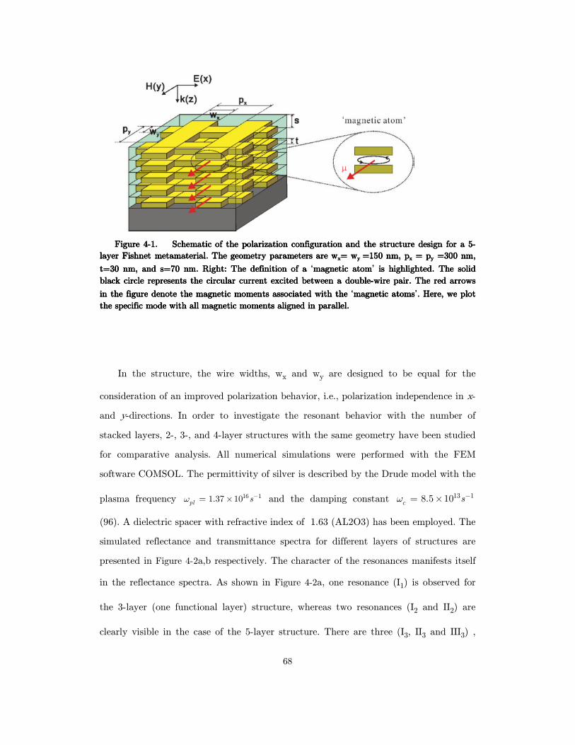
68

Figure Figure Figure Figure 4444----1111. . . . Schematic of the polarization configuration and the structureSchematic of the polarization configuration and the structureSchematic of the polarization configuration and the structureSchematic of the polarization configuration and the structure design for a 5design for a 5design for a 5design for a 5----

layer layer layer layer FishnetFishnetFishnetFishnet metamaterialmetamaterialmetamaterialmetamaterial. The geometry parameters are w. The geometry parameters are w. The geometry parameters are w. The geometry parameters are wxxxx= w= w= w= wy y y y =150 nm, =150 nm, =150 nm, =150 nm, ppppxxxx ==== ppppyyyy ====333300 nm, 00 nm, 00 nm, 00 nm,

tttt====30 nm, and 30 nm, and 30 nm, and 30 nm, and ssss====70 nm. Right: 70 nm. Right: 70 nm. Right: 70 nm. Right: The definition of a The definition of a The definition of a The definition of a ‘magnetic atommagnetic atommagnetic atommagnetic atom’ is highis highis highis highlighted. The solid lighted. The solid lighted. The solid lighted. The solid

black circle black circle black circle black circle represents the circular current excited betwrepresents the circular current excited betwrepresents the circular current excited betwrepresents the circular current excited between a doubleeen a doubleeen a doubleeen a double----wire pair. The red wire pair. The red wire pair. The red wire pair. The red arrows arrows arrows arrows

in the figure denote the magnein the figure denote the magnein the figure denote the magnein the figure denote the magnetic moments associated with the tic moments associated with the tic moments associated with the tic moments associated with the ‘magnetic atomsmagnetic atomsmagnetic atomsmagnetic atoms’. Here, we plot . Here, we plot . Here, we plot . Here, we plot

the the the the specific mode with all magneticspecific mode with all magneticspecific mode with all magneticspecific mode with all magnetic mommommommoments aligned in parallel.ents aligned in parallel.ents aligned in parallel.ents aligned in parallel.

In the structure, the wire widths, wx and wy are designed to be equal for the

consideration of an improved polarization behavior, i.e., polarization independence in x-

and y-directions. In order to investigate the resonant behavior with the number of

stacked layers, 2-, 3-, and 4-layer structures with the same geometry have been studied

for comparative analysis. All numerical simulations were performed with the FEM

software COMSOL. The permittivity of silver is described by the Drude model with the

plasma frequency 16 11.37 10pl sω −= × and the damping constant 13 18.5 10c

sω −= ×

(96). A dielectric spacer with refractive index of 1.63 (AL2O3) has been employed. The

simulated reflectance and transmittance spectra for different layers of structures are

presented in Figure 4-2a,b respectively. The character of the resonances manifests itself

in the reflectance spectra. As shown in Figure 4-2a, one resonance (I1) is observed for

the 3-layer (one functional layer) structure, whereas two resonances (I2 and II2) are

clearly visible in the case of the 5-layer structure. There are three (I3, II3 and III3) ,

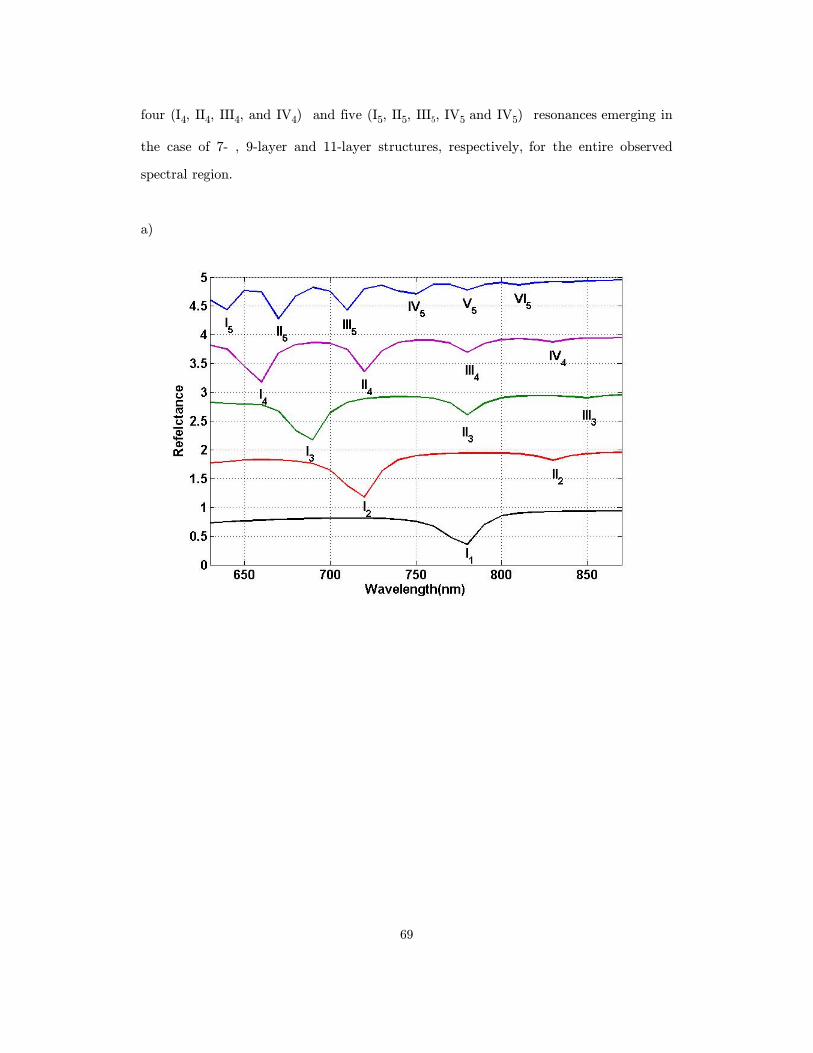
69

four (I4, II4, III4, and IV4) and five (I5, II5, III5, IV5 and IV5) resonances emerging in

the case of 7- , 9-layer and 11-layer structures, respectively, for the entire observed

spectral region.

a)

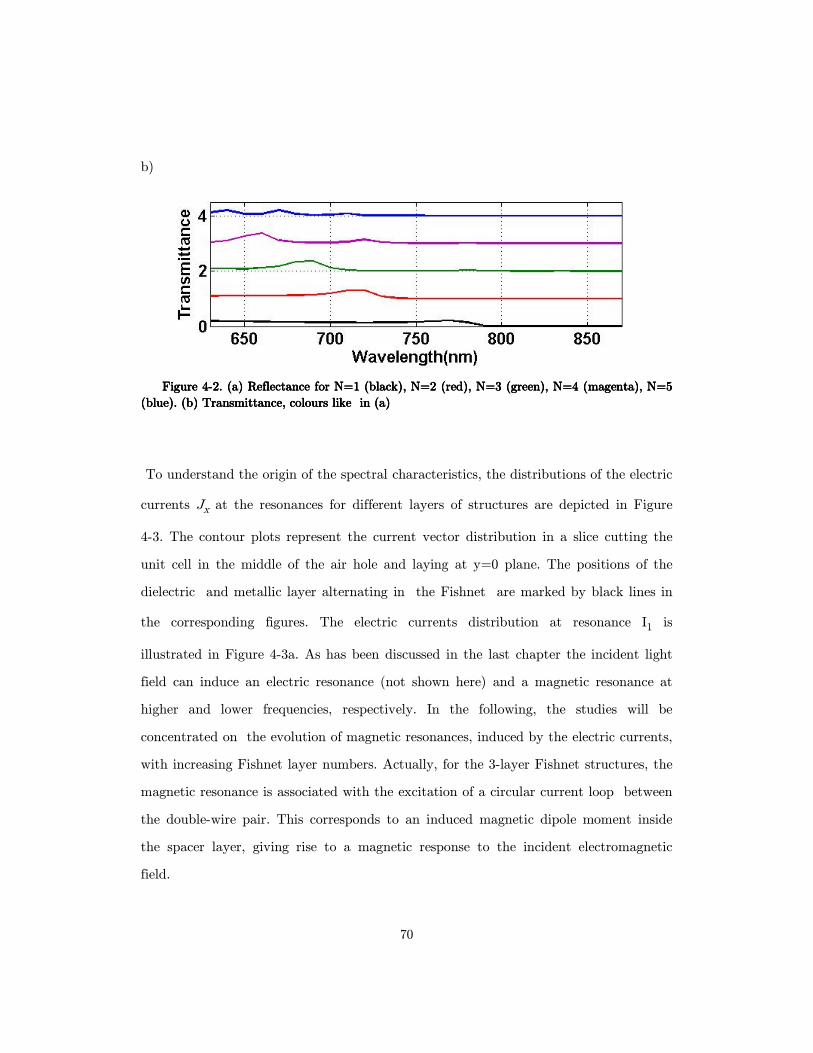
70

b)

Figure Figure Figure Figure 4444----2222. (a) Reflectance for N=. (a) Reflectance for N=. (a) Reflectance for N=. (a) Reflectance for N=1 (black), N=2 (red), N=3 (green), N=4 (magenta), N=5 1 (black), N=2 (red), N=3 (green), N=4 (magenta), N=5 1 (black), N=2 (red), N=3 (green), N=4 (magenta), N=5 1 (black), N=2 (red), N=3 (green), N=4 (magenta), N=5

(blue). (b) Transmittance, colours(blue). (b) Transmittance, colours(blue). (b) Transmittance, colours(blue). (b) Transmittance, colours like in (a)like in (a)like in (a)like in (a)

To understand the origin of the spectral characteristics, the distributions of the electric

currents Jx at the resonances for different layers of structures are depicted in Figure

4-3. The contour plots represent the current vector distribution in a slice cutting the

unit cell in the middle of the air hole and laying at y=0 plane. The positions of the

dielectric and metallic layer alternating in the Fishnet are marked by black lines in

the corresponding figures. The electric currents distribution at resonance I1 is

illustrated in Figure 4-3a. As has been discussed in the last chapter the incident light

field can induce an electric resonance (not shown here) and a magnetic resonance at

higher and lower frequencies, respectively. In the following, the studies will be

concentrated on the evolution of magnetic resonances, induced by the electric currents,

with increasing Fishnet layer numbers. Actually, for the 3-layer Fishnet structures, the

magnetic resonance is associated with the excitation of a circular current loop between

the double-wire pair. This corresponds to an induced magnetic dipole moment inside

the spacer layer, giving rise to a magnetic response to the incident electromagnetic

field.

71

a)

b)

c)

Figure Figure Figure Figure 4444----3333 Simulated electric current of Jx in the plane y=0 at the corresponding resonant Simulated electric current of Jx in the plane y=0 at the corresponding resonant Simulated electric current of Jx in the plane y=0 at the corresponding resonant Simulated electric current of Jx in the plane y=0 at the corresponding resonant

frequencies together with the schematic wavefrequencies together with the schematic wavefrequencies together with the schematic wavefrequencies together with the schematic wave----functions for (A) 1functions for (A) 1functions for (A) 1functions for (A) 1----, (B) 2, (B) 2, (B) 2, (B) 2---- and (C) 3and (C) 3and (C) 3and (C) 3----functional functional functional functional

layer layer layer layer FishnetFishnetFishnetFishnet metamaterialmetamaterialmetamaterialmetamaterials. The grey circles in s. The grey circles in s. The grey circles in s. The grey circles in the schematic drawings represent the the schematic drawings represent the the schematic drawings represent the the schematic drawings represent the ‘magnetic magnetic magnetic magnetic

atomsatomsatomsatoms’....

In analogy to electric plasmons excited in metallic nanostructures, the magnetic dipole

oscillation inside the spacer layer has been defined (112) to be a magnetic plasmon. For

the 5-layer structure, two circulating current loops are induced in the three-wire

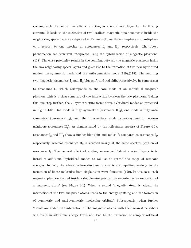
72

system, with the central metallic wire acting as the common layer for the flowing

currents. It leads to the excitation of two localized magnetic dipole moments inside the

neighboring spacer layers as depicted in Figure 4-3b, oscillating in-phase and anti-phase

with respect to one another at resonances I2 and II2, respectively. The above

phenomenon has been well interpreted using the hybridization of magnetic plasmons.

(118) The close proximity results in the coupling between the magnetic plasmons inside

the two neighboring spacer layers and gives rise to the formation of two new hybridized

modes: the symmetric mode and the anti-symmetric mode (119),(118). The resulting

two magnetic resonances I2 and II2 blue-shift and red-shift, respectively, in comparison

to resonance I1, which corresponds to the bare mode of an individual magnetic

plasmon. This is a clear signature of the interaction between the two plasmons. Taking

this one step further, the 7-layer structure forms three hybridized modes as presented

in Figure 4-3c. One mode is fully symmetric (resonance III3), one mode is fully anti-

symmetric (resonance I3), and the intermediate mode is non-symmetric between

neighbors (resonance II3). As demonstrated by the reflectance spectra of Figure 4-2a,

resonances I3 and III3 show a further blue-shift and red-shift compared to resonance I1,

respectively, whereas resonance II3 is situated nearly at the same spectral position of

resonance I1. The general effect of adding successive Fishnet stacked layers is to

introduce additional hybridized modes as well as to spread the range of resonant

energies. In fact, the whole picture discussed above is a compelling analogy to the

formation of linear molecules from single atom wave-functions (120). In this case, each

magnetic plasmon excited inside a double-wire pair can be regarded as an excitation of

a ‘magnetic atom’ (see Figure 4-1). When a second ‘magnetic atom’ is added, the

interaction of the two ‘magnetic atoms’ leads to the energy splitting and the formation

of symmetric and anti-symmetric ‘molecular orbitals’. Subsequently, when further

‘atoms’ are added, the interaction of the ‘magnetic atoms’ with their nearest neighbors

will result in additional energy levels and lead to the formation of complex artificial

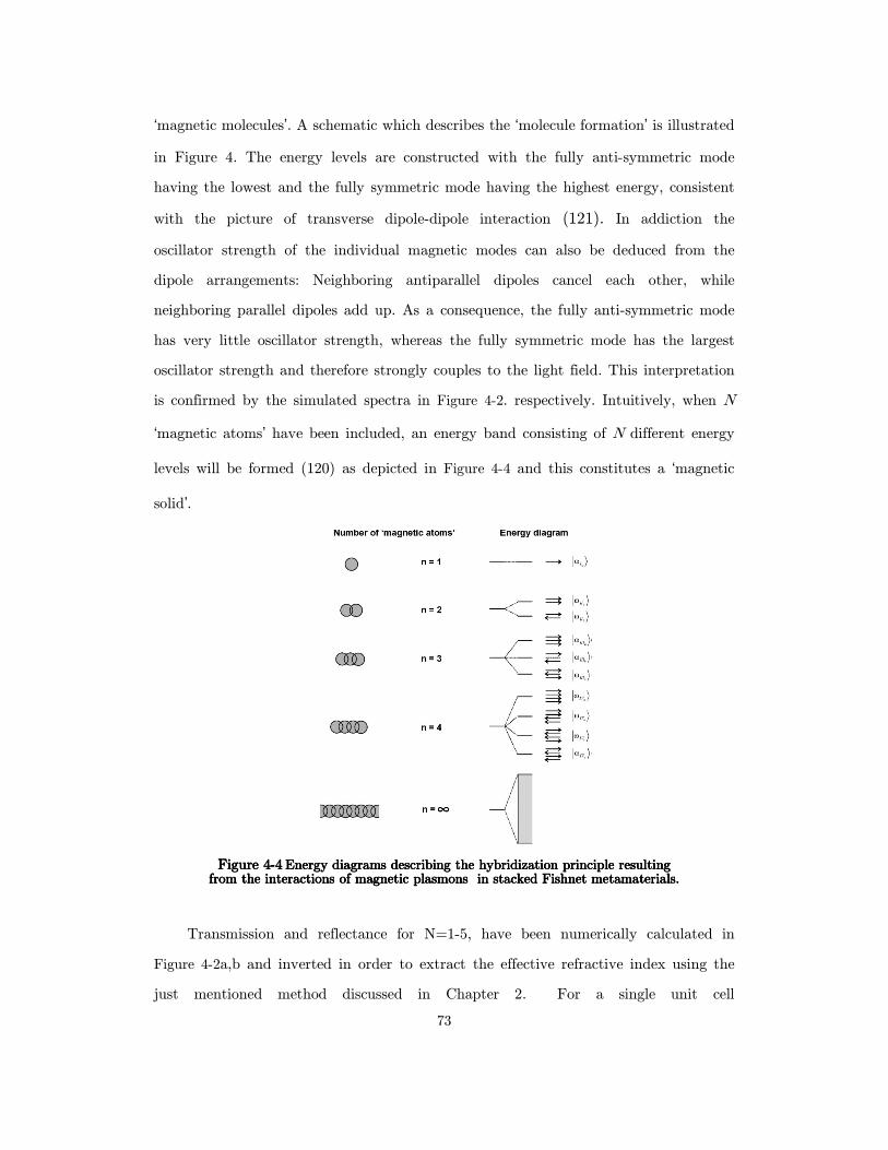
73

‘magnetic molecules’. A schematic which describes the ‘molecule formation’ is illustrated

in Figure 4. The energy levels are constructed with the fully anti-symmetric mode

having the lowest and the fully symmetric mode having the highest energy, consistent

with the picture of transverse dipole-dipole interaction (121). In addiction the

oscillator strength of the individual magnetic modes can also be deduced from the

dipole arrangements: Neighboring antiparallel dipoles cancel each other, while

neighboring parallel dipoles add up. As a consequence, the fully anti-symmetric mode

has very little oscillator strength, whereas the fully symmetric mode has the largest

oscillator strength and therefore strongly couples to the light field. This interpretation

is confirmed by the simulated spectra in Figure 4-2. respectively. Intuitively, when N

‘magnetic atoms’ have been included, an energy band consisting of N different energy

levels will be formed (120) as depicted in Figure 4-4 and this constitutes a ‘magnetic

solid’.

Figure Figure Figure Figure 4444----4444 Energy diagrams describing the hybridization principle resultingEnergy diagrams describing the hybridization principle resultingEnergy diagrams describing the hybridization principle resultingEnergy diagrams describing the hybridization principle resulting from the interactions offrom the interactions offrom the interactions offrom the interactions of magnetic plasmonsmagnetic plasmonsmagnetic plasmonsmagnetic plasmons in stacked in stacked in stacked in stacked FishnetFishnetFishnetFishnet metamaterialmetamaterialmetamaterialmetamaterials.s.s.s.

Transmission and reflectance for N=1-5, have been numerically calculated in

Figure 4-2a,b and inverted in order to extract the effective refractive index using the

just mentioned method discussed in Chapter 2. For a single unit cell

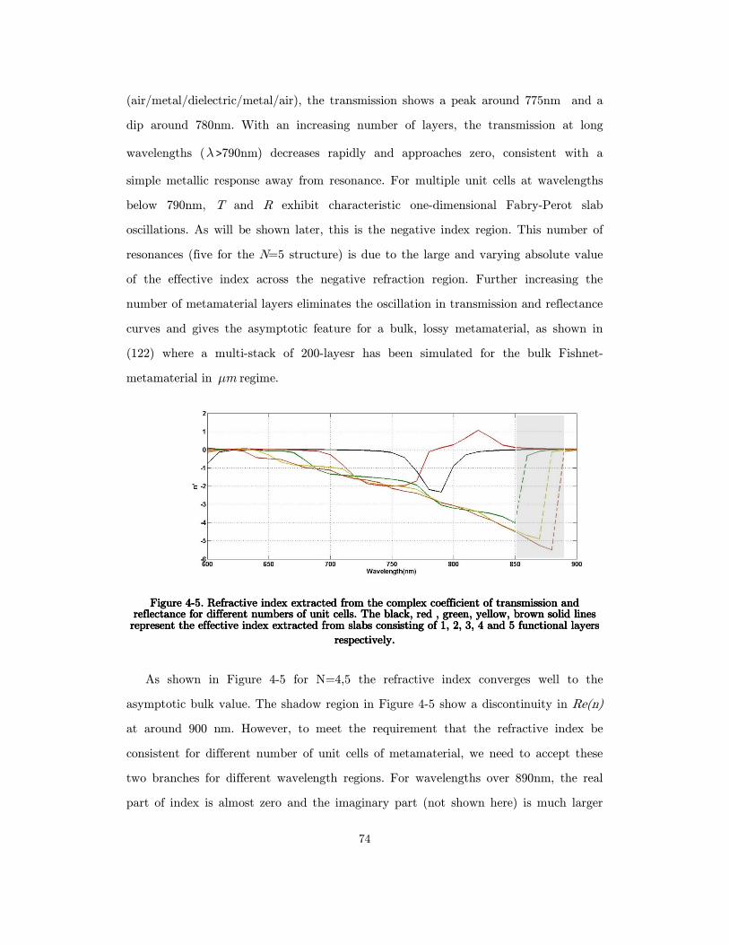
74

(air/metal/dielectric/metal/air), the transmission shows a peak around 775nm and a

dip around 780nm. With an increasing number of layers, the transmission at long

wavelengths (λ >790nm) decreases rapidly and approaches zero, consistent with a

simple metallic response away from resonance. For multiple unit cells at wavelengths

below 790nm, T and R exhibit characteristic one-dimensional Fabry-Perot slab

oscillations. As will be shown later, this is the negative index region. This number of

resonances (five for the N=5 structure) is due to the large and varying absolute value

of the effective index across the negative refraction region. Further increasing the

number of metamaterial layers eliminates the oscillation in transmission and reflectance

curves and gives the asymptotic feature for a bulk, lossy metamaterial, as shown in

(122) where a multi-stack of 200-layesr has been simulated for the bulk Fishnet-

metamaterial in mµ regime.

Figure Figure Figure Figure 4444----5555.... Refractive index extracted from the complex coefficient of transmission and Refractive index extracted from the complex coefficient of transmission and Refractive index extracted from the complex coefficient of transmission and Refractive index extracted from the complex coefficient of transmission and reflectareflectareflectareflectance nce nce nce for different numbers of unit cellfor different numbers of unit cellfor different numbers of unit cellfor different numbers of unit cells. The black, red , green, yellow, brown solid liness. The black, red , green, yellow, brown solid liness. The black, red , green, yellow, brown solid liness. The black, red , green, yellow, brown solid lines represent the effective index extracted represent the effective index extracted represent the effective index extracted represent the effective index extracted from from from from slabs consisting of 1, 2, 3, 4 and 5 functional layersslabs consisting of 1, 2, 3, 4 and 5 functional layersslabs consisting of 1, 2, 3, 4 and 5 functional layersslabs consisting of 1, 2, 3, 4 and 5 functional layers

respectively.respectively.respectively.respectively.

As shown in Figure 4-5 for N=4,5 the refractive index converges well to the

asymptotic bulk value. The shadow region in Figure 4-5 show a discontinuity in Re(n)

at around 900 nm. However, to meet the requirement that the refractive index be

consistent for different number of unit cells of metamaterial, we need to accept these

two branches for different wavelength regions. For wavelengths over 890nm, the real

part of index is almost zero and the imaginary part (not shown here) is much larger

75

than the real part, exhibiting metallic properties. For light propagating in a periodic

structure, an infinite number of modes exist for a given frequency (each mode is the

linear combination of many Floquet plane waves based on the periodicity in the

transverse directions). As the number of unit cells along the propagation direction is

increased, the mode with the smallest imaginary part dominates the optical response

(122),(116). The reason for the discontinuity has been cleared in (122): the imaginary

part of the fundamental mode exceeds that of the first higher mode for wavelengths

above 850nm, and therefore, for a thick slab, the second mode becomes the dominant

mode at longer wavelengths. As shown in Figure 4-5, the effective index calculated for

five to ten layers converges very well except for a narrow wavelength range around

850nm where the two modes exhibit comparable losses, indicating that the fundamental

mode is absolutely dominant over other modes over most of the frequency range (up to

850nm). A modal analysis will be presented in Chapter 6 which reproduces the complex

dispersion curves of the first least-damped modes in such structure.

4.24.24.24.2 The role of surface polaritons in multilayered Fishnet

metamaterial

A surface plasmon polariton (SPP) is an electromagnetic surface wave traveling along

the interface separating a dielectric and a metal. It is produced by the interaction of

collective oscillations of free electrons in the metal surface with the electromagnetic

wave impinging on the metal. The first theoretical description of surface plasmons

dates back to 1957 when Ritchie (123) predicted the existence of surface plasmons

when he discussed the plasma losses in thin films. However, it was in 1998, when

Ebbesen et al. (124) published their pioneering work about Extraordinary Optical

Transmission ˙EOT˙ through hole arrays in metallic films, when SPPs attracted the

attention of fundamental research giving rise to the field of plasmonics. Since then,

other studies have proved the existence of EOT (for a complete review see (125)),

mostly on single-layer metal films with periodic hole arrays, being well accepted that

the EOT through single-layer hole arrays originates from the grating coupling between

76

the dispersion relation of the SPPs that propagate along a smooth infinite metal-

dielectric interface and the momentum of the incident light taking into account the

lattice structure provided by the holes. However, this procedure has to be considered as

an approximation due to the fact that it models the momentum of the SPPs on a holed

array using the expression of SPPs on a smooth metal-dielectric interface, thus ignoring

the effect which the holes may have on the SPP propagation. Nevertheless the

predictions of this model are usually very accurate (126). In the last session the

phenomenological model of ‘magnetic molecules’ has been discussed in order to explain

the distribution of magnetic resonances inside a multi-layered Fishnet metamaterial.

Only the magnetic resonances have been taken into account. Next numerically

studies are carried out to find the correlation (at least in a good approximation)

between all the magnetic resonances of a N= 1,2,3 and 4 functional layers Fishnet

metamaterial. It is known that when two metal layers are placed closer than the SPP

attenuation length, the SPPs that propagate along each of the two inner interfaces

couple to each other, thus creating a mode called internal SPPs whose dispersion

relation differs from the usual aforementioned dispersion relation of the SPPs on a

single interface. In the fellow will be presented, in analogy with the model for single-

layer hole arrays, the dispersion relation of the SPPs propagating on a multilayer

structure without holes and it will be equate with the momentum of the incident light

,taking into account the periodicity of the structure provided by the holes.

In Figure 4-6 the analytic dispersion curves for a 5-layers structure is shown.

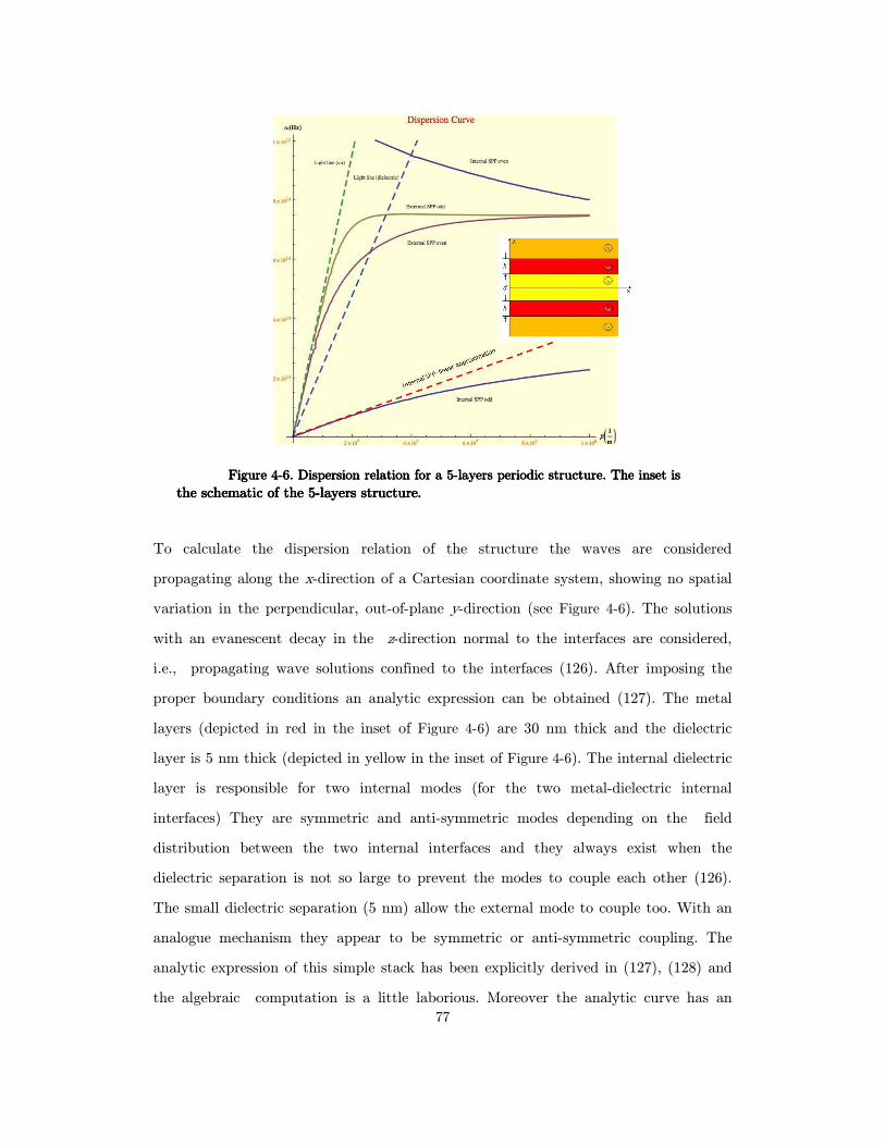
77

Figure Figure Figure Figure 4444----6666. . . . Dispersion relation for a 5Dispersion relation for a 5Dispersion relation for a 5Dispersion relation for a 5----layerlayerlayerlayerssss periodic structure. The inset is periodic structure. The inset is periodic structure. The inset is periodic structure. The inset is

the schematic of the 5the schematic of the 5the schematic of the 5the schematic of the 5----layerlayerlayerlayerssss structure.structure.structure.structure.

To calculate the dispersion relation of the structure the waves are considered

propagating along the x-direction of a Cartesian coordinate system, showing no spatial

variation in the perpendicular, out-of-plane y-direction (see Figure 4-6). The solutions

with an evanescent decay in the z-direction normal to the interfaces are considered,

i.e., propagating wave solutions confined to the interfaces (126). After imposing the

proper boundary conditions an analytic expression can be obtained (127). The metal

layers (depicted in red in the inset of Figure 4-6) are 30 nm thick and the dielectric

layer is 5 nm thick (depicted in yellow in the inset of Figure 4-6). The internal dielectric

layer is responsible for two internal modes (for the two metal-dielectric internal

interfaces) They are symmetric and anti-symmetric modes depending on the field

distribution between the two internal interfaces and they always exist when the

dielectric separation is not so large to prevent the modes to couple each other (126).

The small dielectric separation (5 nm) allow the external mode to couple too. With an

analogue mechanism they appear to be symmetric or anti-symmetric coupling. The

analytic expression of this simple stack has been explicitly derived in (127), (128) and

the algebraic computation is a little laborious. Moreover the analytic curve has an

78

implicit dependence by frequency and wave vector. When more layers have to be taken

into account the computation becomes even challenging. A simple way to overcome the

algebraic computation is to employ a modal analysis for extracting the dispersion

curves in a more straightforward way by simulation. The out-of-plane modes package

in COMSOL has been used. This 2D simulation calculate modes propagating in the

third direction (perpendicular to the computational plane) with periodic boundary

condition in one direction (x-direction for the present case) and with PEC (Perfect

Electric Conductor) condition under and above the unite cell. Once know the way to

simply extract the dispersion curves for a multi-flat layered structure evolving in the z-

direction it’s possible to equal them (in good approximation) to the momentum of the

incident light (tacking into account the periodicity of the structure provided by the

holes).

, , , 0

sinSPP flat SPP holes x i j x yk k k G k iG jGφ= + = + +≃ (4.1)

The second step is to extract the reflection and transmission coefficients of the

multi-layered system. In this way it’s possible to identify the modes of the stacked

structure by equaling its resonant frequencies to the ones of the dispersion curves. The

modal analysis for the flat multi-layered structure and its correlated full vectorial

simulation for multi-layered structure with periodic holes has been performed for 1 up

to 4 functional layers structures with period P=600nm, hole sizes wx, wy =100nm, and

metal (Drude silver)/dielectric (n=1.38) spacers of hm= hd=30nm respectively. In

Figure 4-7 the dispersion relations for a 27-multi-layer structure (N=13) has been

calculated with the modal solver. As predicted by Economu (127) the internal modes of

a multi-layered structure (13 in this case) have a phase velocity

1/2

)exp(2 ) 1 2 cos( )exp(/ 2

exp(2 ) 1

m m p m

d d p

p m

k h ah k hc c h h

k hλ

+ − = + −

ɶ (4.2)

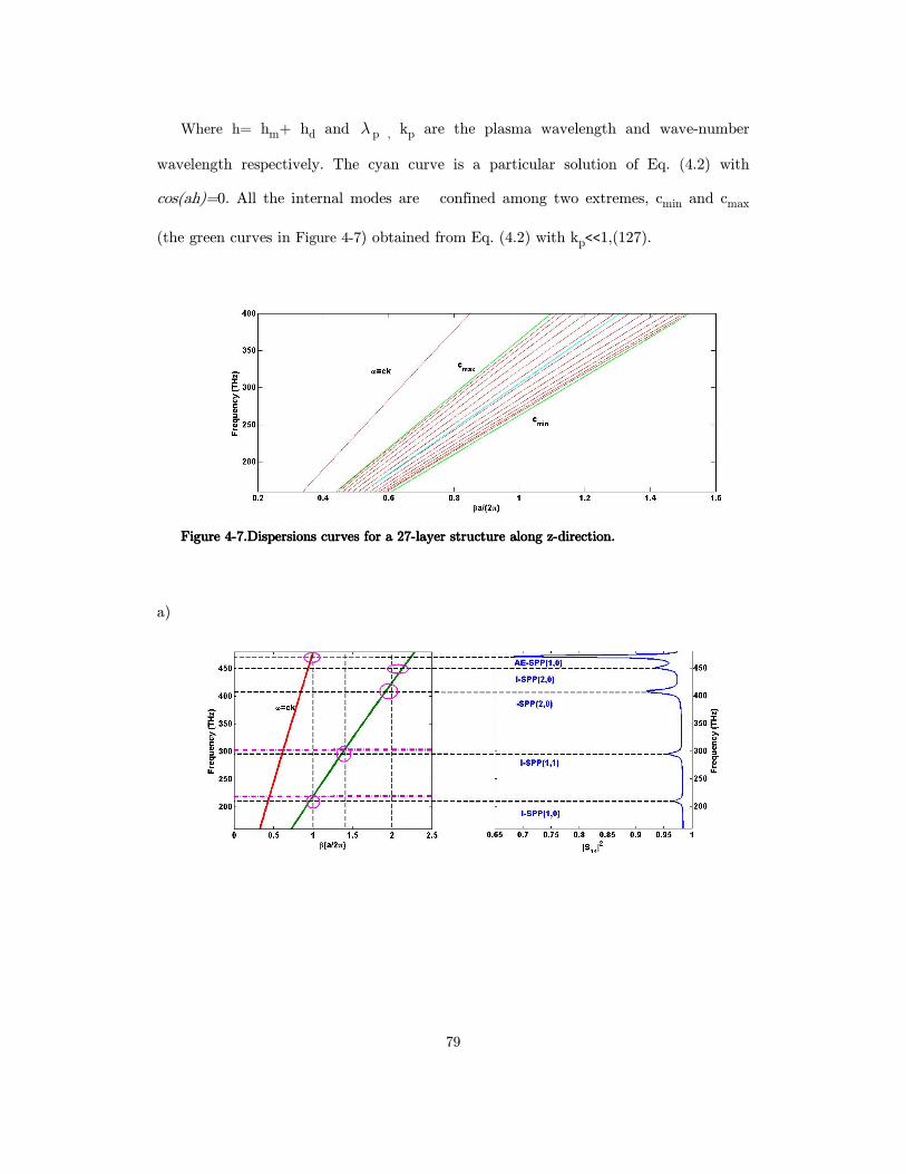
79

Where h= hm+ hd and λ p , kp are the plasma wavelength and wave-number

wavelength respectively. The cyan curve is a particular solution of Eq. (4.2) with

cos(ah)=0. All the internal modes are confined among two extremes, cmin and cmax

(the green curves in Figure 4-7) obtained from Eq. (4.2) with kp<<1,(127).

Figure Figure Figure Figure 4444----7777.Dispersions curves f.Dispersions curves f.Dispersions curves f.Dispersions curves for a 27or a 27or a 27or a 27----layer structure along zlayer structure along zlayer structure along zlayer structure along z----direction.direction.direction.direction.

a)

80

b)

Figure Figure Figure Figure 4444----8888. (a). (a). (a). (a)----left: dispersion relation from the model analysis for a 3left: dispersion relation from the model analysis for a 3left: dispersion relation from the model analysis for a 3left: dispersion relation from the model analysis for a 3----layer layer layer layer structure structure structure structure along along along along

the zthe zthe zthe z----directiondirectiondirectiondirection in the flat casein the flat casein the flat casein the flat case. The red curve is the light curve, the green curve is the dispersion . The red curve is the light curve, the green curve is the dispersion . The red curve is the light curve, the green curve is the dispersion . The red curve is the light curve, the green curve is the dispersion

of the internal modesof the internal modesof the internal modesof the internal modes.... (a)(a)(a)(a)----right: right: right: right: |SSSS11111111|2 parameter for the 3parameter for the 3parameter for the 3parameter for the 3----layer layer layer layer FishnetFishnetFishnetFishnet with periodic holes.with periodic holes.with periodic holes.with periodic holes. (b) (b) (b) (b)

refractive index of 3refractive index of 3refractive index of 3refractive index of 3----layer layer layer layer FishnetFishnetFishnetFishnet metamaterialmetamaterialmetamaterialmetamaterials.s.s.s.

In Figure 4-8a is shown the comparison between the frequencies predicted by the modal

analysis and the resonant frequencies associated to the reflectance deeps for several

values (i,j) of internal (I-SPP) and external (E-SPP) SPP modes. In Figure 4-8a the

predicted frequencies are seen to approximately match the simulated spectra reflectance

deeps (correlated to the EOT peaks) according to Eq. (4.1). Agreement between

simulation and the model is not perfect because the dispersion relation of the SPPs

used as matching condition does not take into account the presence of the holes, which

cause scattering losses and a resonance shift. As a consequence, the predicted resonant

frequencies are slightly larger than those obtained by simulations (128). The magenta

circles mark the frequency region of the matching while the magenta dashed horizontal

lines represent the resonant frequencies for the same model with smaller hole (60nm

thick). In this last case the matching is even better as expected.

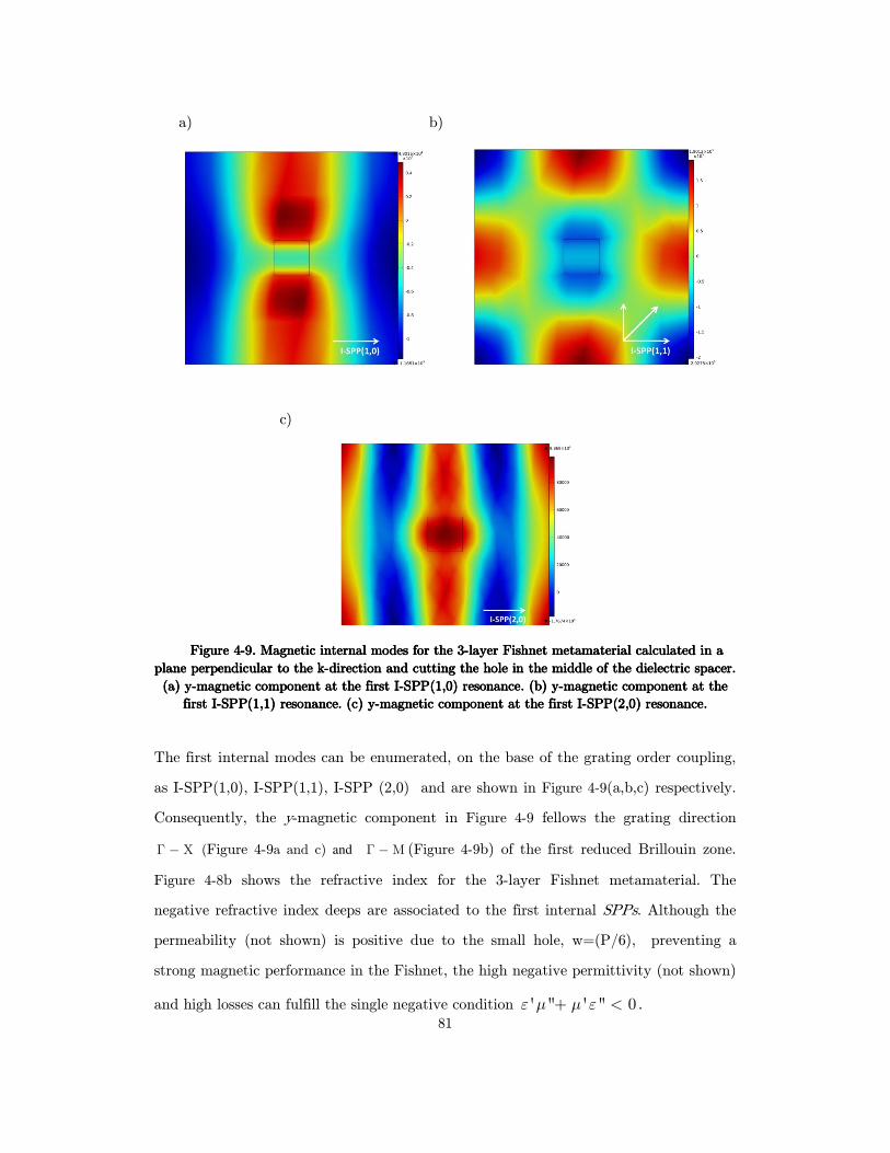
81

a) b)

c)

Figure Figure Figure Figure 4444----9999. Magnetic internal modes for the 3. Magnetic internal modes for the 3. Magnetic internal modes for the 3. Magnetic internal modes for the 3----layer layer layer layer FishnetFishnetFishnetFishnet metamaterialmetamaterialmetamaterialmetamaterial calculated in a calculated in a calculated in a calculated in a

plane perpendicular to the kplane perpendicular to the kplane perpendicular to the kplane perpendicular to the k----direction and cutting the hole in the middle of the dielectric spacer. direction and cutting the hole in the middle of the dielectric spacer. direction and cutting the hole in the middle of the dielectric spacer. direction and cutting the hole in the middle of the dielectric spacer.

(a) y(a) y(a) y(a) y----magnetic component at the first Imagnetic component at the first Imagnetic component at the first Imagnetic component at the first I----SPP(1,0) resonance. (b) ySPP(1,0) resonance. (b) ySPP(1,0) resonance. (b) ySPP(1,0) resonance. (b) y----magnetic component at the magnetic component at the magnetic component at the magnetic component at the

first Ifirst Ifirst Ifirst I----SPP(1,1) resonance. (c) ySPP(1,1) resonance. (c) ySPP(1,1) resonance. (c) ySPP(1,1) resonance. (c) y----magnetic compmagnetic compmagnetic compmagnetic component at the first Ionent at the first Ionent at the first Ionent at the first I----SPP(2,0) resonance.SPP(2,0) resonance.SPP(2,0) resonance.SPP(2,0) resonance.

The first internal modes can be enumerated, on the base of the grating order coupling,

as I-SPP(1,0), I-SPP(1,1), I-SPP (2,0) and are shown in Figure 4-9(a,b,c) respectively.

Consequently, the y-magnetic component in Figure 4-9 fellows the grating direction

Γ − Χ (Figure 4-9a and c) and Γ − Μ (Figure 4-9b) of the first reduced Brillouin zone.

Figure 4-8b shows the refractive index for the 3-layer Fishnet metamaterial. The

negative refractive index deeps are associated to the first internal SPPs. Although the

permeability (not shown) is positive due to the small hole, w=(P/6), preventing a

strong magnetic performance in the Fishnet, the high negative permittivity (not shown)

and high losses can fulfill the single negative condition ' '' ' '' 0ε µ µ ε+ < .

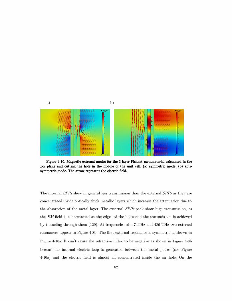
82

a) b)

Figure Figure Figure Figure 4444----10101010. Magnetic external modes for the 3. Magnetic external modes for the 3. Magnetic external modes for the 3. Magnetic external modes for the 3----layer layer layer layer FishnetFishnetFishnetFishnet metamaterialmetamaterialmetamaterialmetamaterial calculated in the calculated in the calculated in the calculated in the

xxxx----k plane and cutting the hole in the middle of the unit cell.k plane and cutting the hole in the middle of the unit cell.k plane and cutting the hole in the middle of the unit cell.k plane and cutting the hole in the middle of the unit cell. (a) symmetric mode, (b) anti(a) symmetric mode, (b) anti(a) symmetric mode, (b) anti(a) symmetric mode, (b) anti----

symmetric mode. The arrow represent the electric field.symmetric mode. The arrow represent the electric field.symmetric mode. The arrow represent the electric field.symmetric mode. The arrow represent the electric field.

The internal SPPs show in general less transmission than the external SPPs as they are

concentrated inside optically thick metallic layers which increase the attenuation due to

the absorption of the metal layer. The external SPPs peak show high transmission, as

the EM field is concentrated at the edges of the holes and the transmission is achieved

by tunneling through them (129). At frequencies of 474THz and 486 THz two external

resonances appear in Figure 4-8b. The first external resonance is symmetric as shown in

Figure 4-10a. It can’t cause the refractive index to be negative as shown in Figure 4-8b

because no internal electric loop is generated between the metal plates (see Figure

4-10a) and the electric field is almost all concentrated inside the air hole. On the

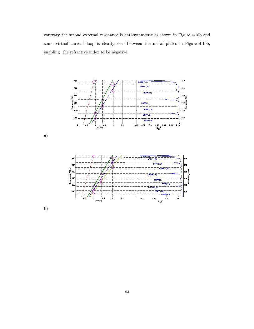
83

contrary the second external resonance is anti-symmetric as shown in Figure 4-10b and

some virtual current loop is clearly seen between the metal plates in Figure 4-10b,

enabling the refractive index to be negative.

a)

b)

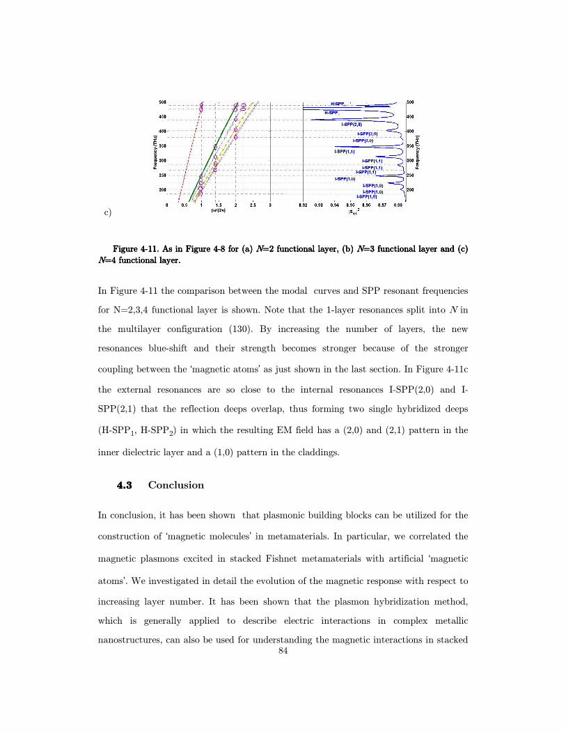
84

c)

Figure Figure Figure Figure 4444----11111111. As in . As in . As in . As in Figure Figure Figure Figure 4444----8888 for (a) for (a) for (a) for (a) NNNN=2 functional layer, (b) =2 functional layer, (b) =2 functional layer, (b) =2 functional layer, (b) NNNN=3 functional layer and (c) =3 functional layer and (c) =3 functional layer and (c) =3 functional layer and (c)

NNNN=4 functional layer. =4 functional layer. =4 functional layer. =4 functional layer.

In Figure 4-11 the comparison between the modal curves and SPP resonant frequencies

for N=2,3,4 functional layer is shown. Note that the 1-layer resonances split into N in

the multilayer configuration (130). By increasing the number of layers, the new

resonances blue-shift and their strength becomes stronger because of the stronger

coupling between the ‘magnetic atoms’ as just shown in the last section. In Figure 4-11c

the external resonances are so close to the internal resonances I-SPP(2,0) and I-

SPP(2,1) that the reflection deeps overlap, thus forming two single hybridized deeps

(H-SPP1, H-SPP2) in which the resulting EM field has a (2,0) and (2,1) pattern in the

inner dielectric layer and a (1,0) pattern in the claddings.

4.34.34.34.3 Conclusion

In conclusion, it has been shown that plasmonic building blocks can be utilized for the

construction of ‘magnetic molecules’ in metamaterials. In particular, we correlated the

magnetic plasmons excited in stacked Fishnet metamaterials with artificial ‘magnetic

atoms’. We investigated in detail the evolution of the magnetic response with respect to

increasing layer number. It has been shown that the plasmon hybridization method,

which is generally applied to describe electric interactions in complex metallic

nanostructures, can also be used for understanding the magnetic interactions in stacked

85

Fishnet metamaterials. This allowed us to classify and explain the rather complex

spectra in the case of up to 3-functional layered Fishnet metamaterials. More

specifically, the interaction of the magnetic plasmons or namely ‘magnetic atoms’ leads

to the formation of artificial ‘magnetic molecules’, following the same hybridization

mechanism of simple atoms bonded into linear molecules. An easy scheme for

evaluating the oscillator strength of different coupled modes was proven to be

applicable. Moreover it has been obtained analytically the dispersion relation of SPPs

in a double-layer metallic structure and it has been shown by numerical analysis that

light coupling to the external and internal SPPs originates EOT. A good matching

between the theoretical and simulated resonant frequencies is observed. In addition, at

the internal-SPP resonant frequencies a negative effective permeability is achieved as a

virtual current loop is formed between the metallic layers which can be used to design

negative-index metamaterials. Understanding the coupling of evanescent waves in

complex double-layer metallic hole arrays nanostructures is of fundamental interest and

practical importance in designing optical devices that could become important building

blocks in future nano-optical systems.

86

5 Experimental Fishnet

In the recent years metamaterials have attracted more and more interest in the

scientific community. A first example of a material with a negative index was

represented by the split-ring resonators (SRRs). Such magnetic structures were realized

in the spectral range from microwave up to 200 THz. To create a metamaterial at

optical wavelengths other structures were proposed [13], however in all the cases small

periodicities (about 300 nm and less) and tiny feature sizes (about 30 nm) are essential.

Thus, the fabrication of optical metamaterials is challenging since high-precision, high-

throughput, and low-cost manufacturing processes are needed. Feature sizes can require

nanofabrication processes with sub-100-nm resolution. For rapid prototyping of

metamaterials, focused-ion beam milling techniques can be used. In FIB, a focused

beam of gallium ions is used to sputter atoms from the surface and it is used as a

micro-machining tool, to pattern materials at the micro and nano-scale. Recently, this

technique was used for fabricating magnetic metamaterials based on split-ring

resonators (131). In order to get the resonance wavelength down to NIR/Vis range the

structure requires sub-100-nm gap sizes (down to 35 nm). For such small features,

EBL-based fabrication requires time consuming tests and careful optimization of

writing parameters and processing steps, leading to relatively long overall fabrication

times. In contrast, the rapid prototyping of complete structures can be achieved via

FIB writing. In fact, although the E-beam lithographic step is faster, with FIB writing

the structure is ready and no further post-processing steps are required. However, due

to the low throughput, FIB has certain limitation in its use for fabricating optical

metamaterials. However, it should be mentioned that for some specific designs and

proof-of-principle experiments, for example including nonlinear materials, FIB is the

first choice for rapid prototyping.

Here we report on the FIB fabrication of “fish-net” structured metamaterial that

shows a resonance in the NIR spectral range. The fish-net structure was previously

proposed by several authors and demonstrate interesting properties for an easy design

87

of an effective negative index material (NIMs). FEM simulations have been used to

design the optimized system and the prepared samples have been analysed by means of

transmittance and reflectance measurements in order to verify the presence of the

resonance.

5.15.15.15.1 Experimental methods

The fabrication of nano-holes array, also called “fish-net” structure requires few step

of process: e-beam evaporation; spin-coating and focused ion beam lithography. A

schematic illustration of the prepared structure is reported in Figure 5-1.

Figure Figure Figure Figure 5555----1111. Unit cell. Unit cell. Unit cell. Unit cell

A suitable substrate for this metamaterial must be transparent in the spectral

region of interest. A soda-lime glass covered with 110nm of ITO was used. The ITO

layer ensures a good adhesion for the coatings to be prepared in a 3 layers stack. Our

design comprises 30nm of Gold (Au) / 50nm of dielectric (n=2.2 ; k=0) / 30nm of

Gold. Au evaporations were performed by means of e-beam, while the interlayer of

dielectric was prepared via sol-gel. The film stack was then patterned by Focused Ion

Beam lithography. An array of 400μm x 400μm was prepared by using an accelerating

voltage of 30kV and a probe current of 28pA. The period was fixed at 780nm while two

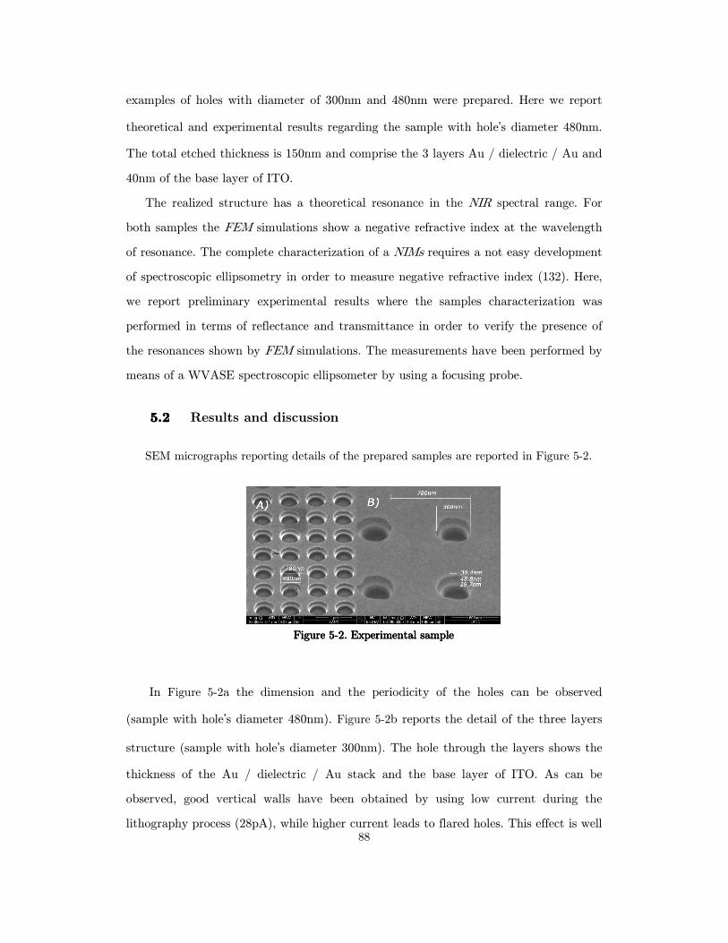
88

examples of holes with diameter of 300nm and 480nm were prepared. Here we report

theoretical and experimental results regarding the sample with hole’s diameter 480nm.

The total etched thickness is 150nm and comprise the 3 layers Au / dielectric / Au and

40nm of the base layer of ITO.

The realized structure has a theoretical resonance in the NIR spectral range. For

both samples the FEM simulations show a negative refractive index at the wavelength

of resonance. The complete characterization of a NIMs requires a not easy development

of spectroscopic ellipsometry in order to measure negative refractive index (132). Here,

we report preliminary experimental results where the samples characterization was

performed in terms of reflectance and transmittance in order to verify the presence of

the resonances shown by FEM simulations. The measurements have been performed by

means of a WVASE spectroscopic ellipsometer by using a focusing probe.

5.25.25.25.2 Results and discussion

SEM micrographs reporting details of the prepared samples are reported in Figure 5-2.

Figure Figure Figure Figure 5555----2222. Experimental sample. Experimental sample. Experimental sample. Experimental sample

In Figure 5-2a the dimension and the periodicity of the holes can be observed

(sample with hole’s diameter 480nm). Figure 5-2b reports the detail of the three layers

structure (sample with hole’s diameter 300nm). The hole through the layers shows the

thickness of the Au / dielectric / Au stack and the base layer of ITO. As can be

observed, good vertical walls have been obtained by using low current during the

lithography process (28pA), while higher current leads to flared holes. This effect is well

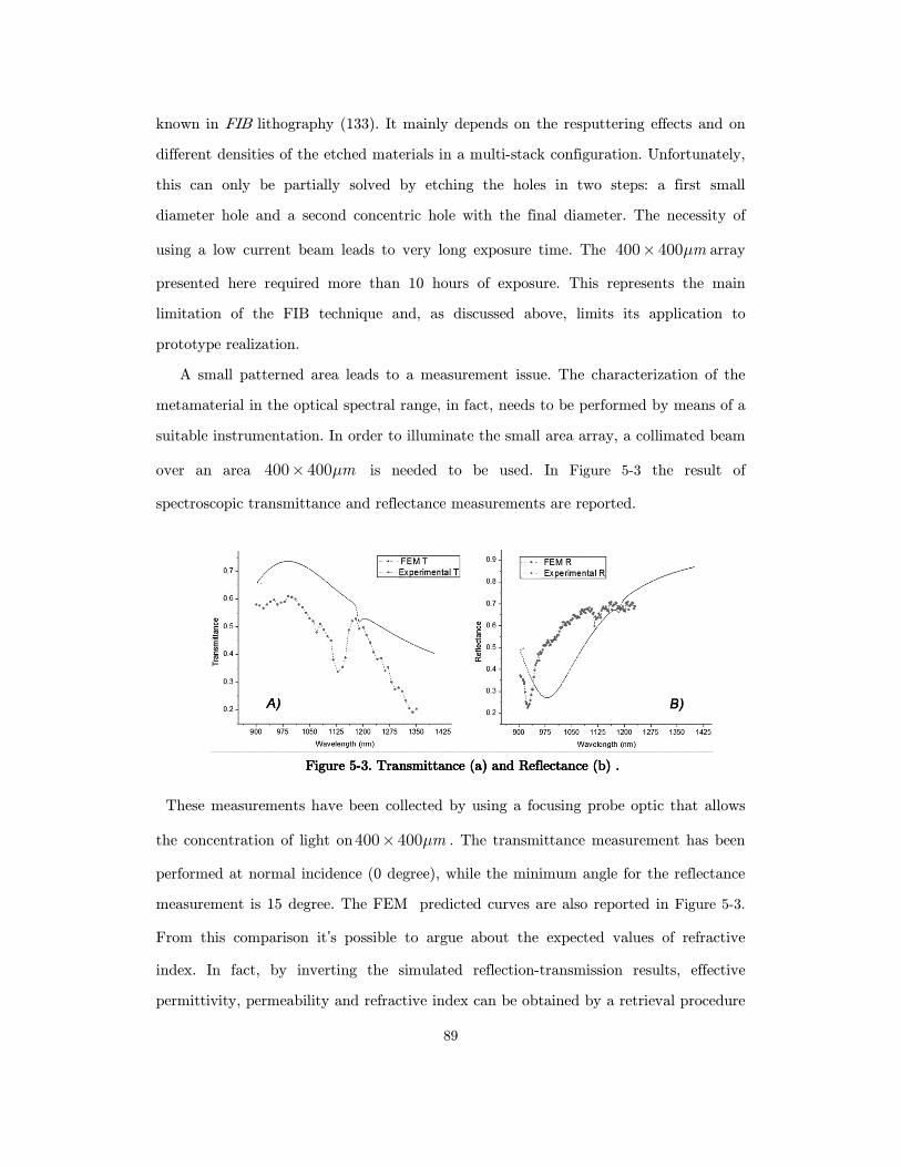
89

known in FIB lithography (133). It mainly depends on the resputtering effects and on

different densities of the etched materials in a multi-stack configuration. Unfortunately,

this can only be partially solved by etching the holes in two steps: a first small

diameter hole and a second concentric hole with the final diameter. The necessity of

using a low current beam leads to very long exposure time. The 400 400 mµ× array

presented here required more than 10 hours of exposure. This represents the main

limitation of the FIB technique and, as discussed above, limits its application to

prototype realization.

A small patterned area leads to a measurement issue. The characterization of the

metamaterial in the optical spectral range, in fact, needs to be performed by means of a

suitable instrumentation. In order to illuminate the small area array, a collimated beam

over an area 400 400 mµ× is needed to be used. In Figure 5-3 the result of

spectroscopic transmittance and reflectance measurements are reported.

Figure Figure Figure Figure 5555----3333.... Transmittance (a) and Reflectance (b) .Transmittance (a) and Reflectance (b) .Transmittance (a) and Reflectance (b) .Transmittance (a) and Reflectance (b) .

These measurements have been collected by using a focusing probe optic that allows

the concentration of light on400 400 mµ× . The transmittance measurement has been

performed at normal incidence (0 degree), while the minimum angle for the reflectance

measurement is 15 degree. The FEM predicted curves are also reported in Figure 5-3.

From this comparison it’s possible to argue about the expected values of refractive

index. In fact, by inverting the simulated reflection-transmission results, effective

permittivity, permeability and refractive index can be obtained by a retrieval procedure

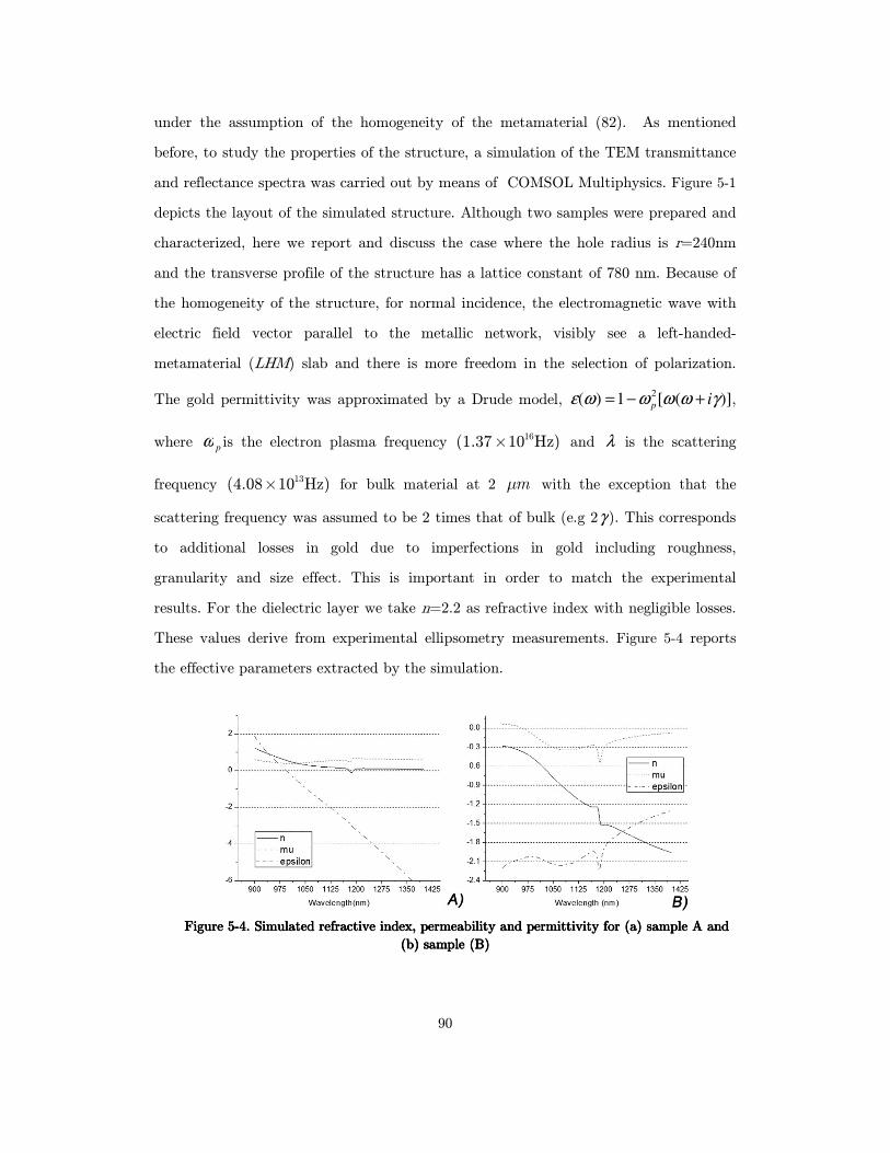
90

under the assumption of the homogeneity of the metamaterial (82). As mentioned

before, to study the properties of the structure, a simulation of the TEM transmittance

and reflectance spectra was carried out by means of COMSOL Multiphysics. Figure 5-1

depicts the layout of the simulated structure. Although two samples were prepared and

characterized, here we report and discuss the case where the hole radius is r=240nm

and the transverse profile of the structure has a lattice constant of 780 nm. Because of

the homogeneity of the structure, for normal incidence, the electromagnetic wave with

electric field vector parallel to the metallic network, visibly see a left-handed-

metamaterial (LHM) slab and there is more freedom in the selection of polarization.

The gold permittivity was approximated by a Drude model, ε(ω) =1−ω p

2[ω(ω + iγ )],

where ω p is the electron plasma frequency × 16(1.37 10 Hz) and λ is the scattering

frequency × 13(4.08 10 Hz) for bulk material at 2 mµ with the exception that the

scattering frequency was assumed to be 2 times that of bulk (e.g 2γ ). This corresponds

to additional losses in gold due to imperfections in gold including roughness,

granularity and size effect. This is important in order to match the experimental

results. For the dielectric layer we take n=2.2 as refractive index with negligible losses.

These values derive from experimental ellipsometry measurements. Figure 5-4 reports

the effective parameters extracted by the simulation.

Figure Figure Figure Figure 5555----4444. Simulated refractive index, permeability and permittivity for (a) sample A and . Simulated refractive index, permeability and permittivity for (a) sample A and . Simulated refractive index, permeability and permittivity for (a) sample A and . Simulated refractive index, permeability and permittivity for (a) sample A and

(b) sample (B)(b) sample (B)(b) sample (B)(b) sample (B)

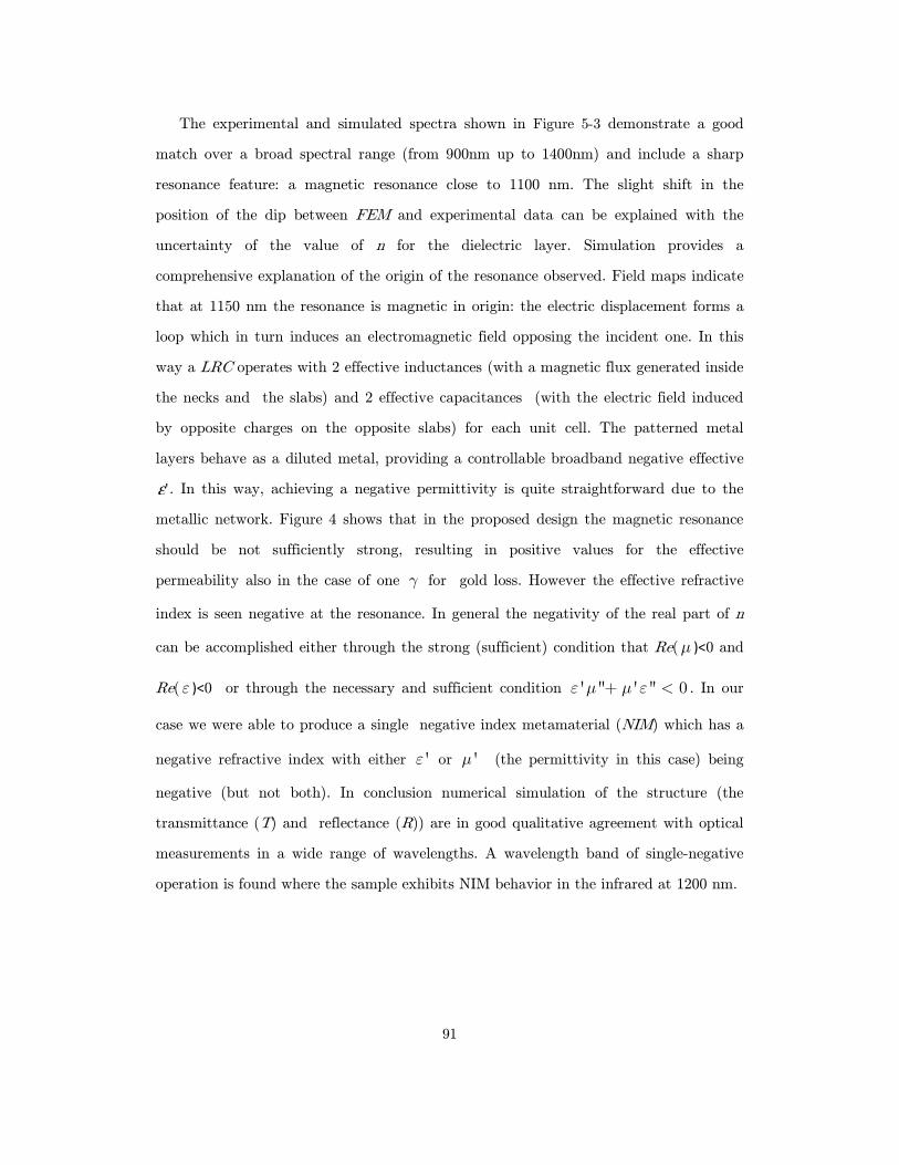
91

The experimental and simulated spectra shown in Figure 5-3 demonstrate a good

match over a broad spectral range (from 900nm up to 1400nm) and include a sharp

resonance feature: a magnetic resonance close to 1100 nm. The slight shift in the

position of the dip between FEM and experimental data can be explained with the

uncertainty of the value of n for the dielectric layer. Simulation provides a

comprehensive explanation of the origin of the resonance observed. Field maps indicate

that at 1150 nm the resonance is magnetic in origin: the electric displacement forms a

loop which in turn induces an electromagnetic field opposing the incident one. In this

way a LRC operates with 2 effective inductances (with a magnetic flux generated inside

the necks and the slabs) and 2 effective capacitances (with the electric field induced

by opposite charges on the opposite slabs) for each unit cell. The patterned metal

layers behave as a diluted metal, providing a controllable broadband negative effective

ε'. In this way, achieving a negative permittivity is quite straightforward due to the

metallic network. Figure 4 shows that in the proposed design the magnetic resonance

should be not sufficiently strong, resulting in positive values for the effective

permeability also in the case of one γ for gold loss. However the effective refractive

index is seen negative at the resonance. In general the negativity of the real part of n

can be accomplished either through the strong (sufficient) condition that Re(µ )<0 and

Re( ε )<0 or through the necessary and sufficient condition ' '' ' '' 0ε µ µ ε+ < . In our

case we were able to produce a single negative index metamaterial (NIM) which has a

negative refractive index with either 'ε or 'µ (the permittivity in this case) being

negative (but not both). In conclusion numerical simulation of the structure (the

transmittance (T) and reflectance (R)) are in good qualitative agreement with optical

measurements in a wide range of wavelengths. A wavelength band of single-negative

operation is found where the sample exhibits NIM behavior in the infrared at 1200 nm.

92

5.35.35.35.3 Bianisotropy Fishnet metamaterial.

The present fabrication techniques for making one- to multiple-functional layer NIMs,

include interferometric lithography (IL) (134), E-beam lithography (EBL) (135),

focused ion beam (FIB) (115), nanoimprint (NIL) (136), and so on. In general, the

processing procedure to fabricate the Fishnet NIMs is to define the hole-size using a

polymetric material, usually by lithographically defining polymer posts, followed by

deposition of the constitutive materials and dissolution of the polymer (liftoff

processing). This processing (fabrication of posts, multi-layer deposition, liftoff) often

gives rise to significant sidewall-angles (SWAs), resulting from continuous growth of

the tops of the posts during the deposition. NIMs with SWAs are not symmetric

structures, but rather are bianisotropic, exhibiting different reflectivities at normal

incidence from the two sides of the film stack. This fabrication induced SWA effect

requires a modified method to retrieve the effective parameters (84),(85) in place of

the conventional approach that is appropriate only to symmetric, vertical sidewall

structures (81). The FEM approach is used to simulate an Ag (silver) – AL2O3

(n=1.63) - Ag sandwich Fishnet structure with 1- and 3-functional layers (FLs). No

substrate is present in the simulation to allow clearer demonstration of the effects of

the bianisotropy. The geometrical parameters of the multi-functional layered Fishnet

NIMs are indicated in tilted view in Figure 5-5. The orthogonal pitches of the 2D

gratings px (pitch along x-axis) and py (pitch along y-axis) are both fixed at 300 nm.

The thicknesses of Ag/AL2O3/Ag are fixed at 30/40/30 nm, respectively. The wx and

wy are both fixed at 75nm. In this way the structure is independent by the incident

wave polarization (in the x-y plane)

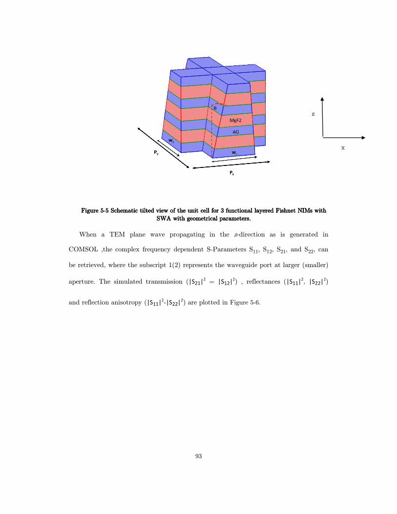
93

Figure Figure Figure Figure 5555----5555 Schematic tilted view of the unit cell for 3 functional layered Schematic tilted view of the unit cell for 3 functional layered Schematic tilted view of the unit cell for 3 functional layered Schematic tilted view of the unit cell for 3 functional layered FishnetFishnetFishnetFishnet NIMs withNIMs withNIMs withNIMs with

SWA with geometrical parameters. SWA with geometrical parameters. SWA with geometrical parameters. SWA with geometrical parameters.

When a TEM plane wave propagating in the z-direction as is generated in

COMSOL ,the complex frequency dependent S-Parameters S11, S12, S21, and S22, can

be retrieved, where the subscript 1(2) represents the waveguide port at larger (smaller)

aperture. The simulated transmission (|S21|2 = |S12|

2) , reflectances (|S11|2, |S22|

2)

and reflection anisotropy (|S11|2-|S22|

2) are plotted in Figure 5-6.

z

x

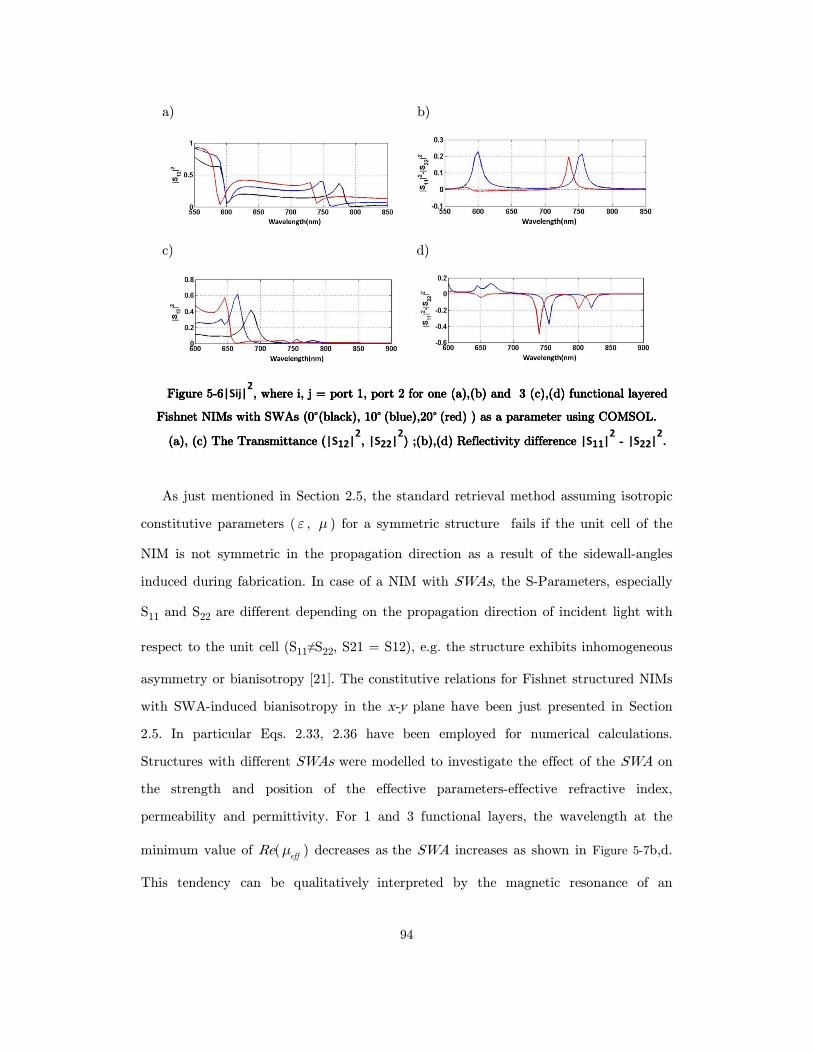
94

a) b)

c) d)

Figure Figure Figure Figure 5555----6666|Sij|2, where i, j = port 1, port 2 for one , where i, j = port 1, port 2 for one , where i, j = port 1, port 2 for one , where i, j = port 1, port 2 for one (a),(b) (a),(b) (a),(b) (a),(b) and 3and 3and 3and 3 (c),(d) (c),(d) (c),(d) (c),(d) functional layered functional layered functional layered functional layered

FishnetFishnetFishnetFishnet NIMs with SWAs (0NIMs with SWAs (0NIMs with SWAs (0NIMs with SWAs (0°(black)(black)(black)(black),,,, 10101010° (blue)(blue)(blue)(blue),20,20,20,20° (red)(red)(red)(red) ) as a parameter using COMSOL. ) as a parameter using COMSOL. ) as a parameter using COMSOL. ) as a parameter using COMSOL.

((((aaaa), (c) The Transmittance (), (c) The Transmittance (), (c) The Transmittance (), (c) The Transmittance (|S12|2, , , , |S22|

2) ;(b),) ;(b),) ;(b),) ;(b),(d) Reflectivity(d) Reflectivity(d) Reflectivity(d) Reflectivity difference difference difference difference |S11|

2 ---- |S22|

2....

As just mentioned in Section 2.5, the standard retrieval method assuming isotropic

constitutive parameters ( ε , µ ) for a symmetric structure fails if the unit cell of the

NIM is not symmetric in the propagation direction as a result of the sidewall-angles

induced during fabrication. In case of a NIM with SWAs, the S-Parameters, especially

S11 and S22 are different depending on the propagation direction of incident light with

respect to the unit cell (S11≠S22, S21 = S12), e.g. the structure exhibits inhomogeneous

asymmetry or bianisotropy [21]. The constitutive relations for Fishnet structured NIMs

with SWA-induced bianisotropy in the x-y plane have been just presented in Section

2.5. In particular Eqs. 2.33, 2.36 have been employed for numerical calculations.

Structures with different SWAs were modelled to investigate the effect of the SWA on

the strength and position of the effective parameters-effective refractive index,

permeability and permittivity. For 1 and 3 functional layers, the wavelength at the

minimum value of Re(effµ ) decreases as the SWA increases as shown in Figure 5-7b,d.

This tendency can be qualitatively interpreted by the magnetic resonance of an

95

equivalent LC circuit: a larger SWA corresponds to smaller capacitance and inductance

(137), which in turn leads to a shorter resonance wavelength.

a) b)

c) d)

Figure Figure Figure Figure 5555----7777.... Real parts of the effective parameters (n, Real parts of the effective parameters (n, Real parts of the effective parameters (n, Real parts of the effective parameters (n, µ and and and and ε) for one) for one) for one) for one----(a,b) and three(a,b) and three(a,b) and three(a,b) and three----(c,d) (c,d) (c,d) (c,d) functionalfunctionalfunctionalfunctional layeredlayeredlayeredlayered FishnetFishnetFishnetFishnet NIMs with SWAs NIMs with SWAs NIMs with SWAs NIMs with SWAs (0(0(0(0°(black)(black)(black)(black), 10, 10, 10, 10° (blue)(blue)(blue)(blue),,,, 20202020°(red)(red)(red)(red) ) using the using the using the using the

modifimodifimodifimodified retrieval equation. (a)ed retrieval equation. (a)ed retrieval equation. (a)ed retrieval equation. (a),(c),(c),(c),(c) showshowshowshowssss Re[Re[Re[Re[nnnneffeffeffeff] and (b)] and (b)] and (b)] and (b),(d),(d),(d),(d) shows shows shows shows Re[ Re[ Re[ Re[ μeff] ] ] ] and Re[and Re[and Re[and Re[εeff]]]]. . . .

The magnitude of negative refractive index in NIMs with 1 FL depends on the

sidewall-angle, that is, the minimum value of Re(effn ) increases as the SWA increases

as shown in Figure 3-7a. The reason for the increase is clear: as the sidewall-angle

increases, the absolute values of Re(effε ) decreases (as shown in Figure 5-7b,d) due to

the decrease of the Ag line-width along the direction of electric field. The wavelength at

the minimum of Re(effn )] decreases with increase of sidewall-angle, which is a result of

the blue-shifted resonance peaks of both Re(effε ) and Re(

effµ ). Also, the blue-shifted

resonance frequency of effective permittivity and permeability as mentioned above

accounts for decrease of the wavelength at minimum effective refractive index in multi-

functional layered NIMs with the increase of the side-wall angle. Moreover Figure 5-8

96

shows that the bi-anisotropic parameter 0ξ for multiple functional layered Fishnet

NIMs as a function of the sidewall-angle.

Figure Figure Figure Figure 5555----8888.... Real and imaginary parts of the biReal and imaginary parts of the biReal and imaginary parts of the biReal and imaginary parts of the bi----anisotropic parameter (anisotropic parameter (anisotropic parameter (anisotropic parameter ( 0ξ ) for one) for one) for one) for one---- (left) and (left) and (left) and (left) and

to five (right) functional layered to five (right) functional layered to five (right) functional layered to five (right) functional layered FishnetFishnetFishnetFishnet NIMs with SWAs (10NIMs with SWAs (10NIMs with SWAs (10NIMs with SWAs (10° blue)blue)blue)blue),20,20,20,20° (red)(red)(red)(red)).).).).

As shown in Figure 5-7d the wavelength of the minimum value of Re(effµ ) is linearly

dependent on the SWA. The trend of a decreasing minimum value of Re(effµ ) can be

explained as a more complicated coupling between magnetic and electric dipoles. In an

ideal Fishnet structured NIM with vertical sidewalls the bianisotropic parameter 0ξ for

Fishnet NIMs with zero sidewall-angle is identically zero, independent of number of

functional layers. The structure is composed of independent electric atoms and

magnetic atoms: the electric response results from the array of thin metal wires parallel

to the electric field direction and the magnetic response from pairs of metal stripes

separated by a dielectric spacer along the direction of magnetic field that support an

anti-symmetric current as shown in Figure 5-9. However, in realistic Fishnet structured

NIMs with a fabrication-induced side wall angle, the NIMs are bianisotropic (138). In

the thin metal wires (electric response), a magnetic dipole in the x-direction is induced

by an electric field EEEE in the y-direction, resulting from the disparity of the current

distribution in the two metal films, so the magnetic and electric dipoles induced by E E E E

are coupled to each other. Similarly, the electric dipoles induced by HHHH (magnetic loop

response) now include a net y-component, so the electric and magnetic dipoles induced

by HHHH are also mutually coupled as shown in Figure 5-9.

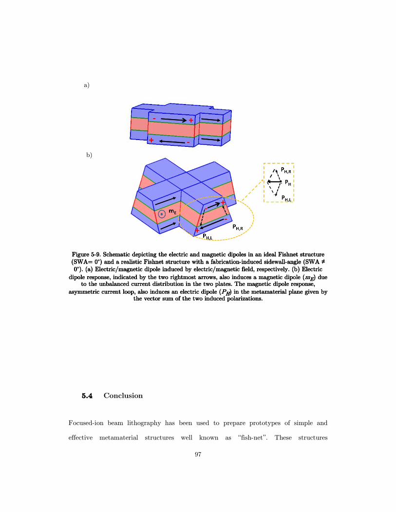
97

Figure Figure Figure Figure 5555----9999.... Schematic depicting the electric and magnetic dipoles in Schematic depicting the electric and magnetic dipoles in Schematic depicting the electric and magnetic dipoles in Schematic depicting the electric and magnetic dipoles in an ideal an ideal an ideal an ideal FishnetFishnetFishnetFishnet structure structure structure structure (SWA= 0(SWA= 0(SWA= 0(SWA= 0°) and a realistic ) and a realistic ) and a realistic ) and a realistic FishnetFishnetFishnetFishnet structure with a fabricationstructure with a fabricationstructure with a fabricationstructure with a fabrication----induced sidewallinduced sidewallinduced sidewallinduced sidewall----angle (SWA angle (SWA angle (SWA angle (SWA ≠ 0000°). (a) ). (a) ). (a) ). (a) Electric/magnetic dipole induced by electric/magnetic field, reElectric/magnetic dipole induced by electric/magnetic field, reElectric/magnetic dipole induced by electric/magnetic field, reElectric/magnetic dipole induced by electric/magnetic field, respectively. (b) Electric spectively. (b) Electric spectively. (b) Electric spectively. (b) Electric

dipole dipole dipole dipole response, indicated by the two rightmost arrows, also induces a magnetic dipole (response, indicated by the two rightmost arrows, also induces a magnetic dipole (response, indicated by the two rightmost arrows, also induces a magnetic dipole (response, indicated by the two rightmost arrows, also induces a magnetic dipole (mmmmEEEE) due ) due ) due ) due to to to to the the the the unbalanced current distribution in the two plates. The magneunbalanced current distribution in the two plates. The magneunbalanced current distribution in the two plates. The magneunbalanced current distribution in the two plates. The magnetic dipole response, tic dipole response, tic dipole response, tic dipole response,

asymmetric asymmetric asymmetric asymmetric current loop, also induces an electric dipole (current loop, also induces an electric dipole (current loop, also induces an electric dipole (current loop, also induces an electric dipole (PPPPHHHH) in the ) in the ) in the ) in the metamaterialmetamaterialmetamaterialmetamaterial plane given plane given plane given plane given by by by by tttthe vector he vector he vector he vector sum of the two induced polarizations.sum of the two induced polarizations.sum of the two induced polarizations.sum of the two induced polarizations.

5.45.45.45.4 Conclusion

Focused-ion beam lithography has been used to prepare prototypes of simple and

effective metamaterial structures well known as ‘‘fish-net’’. These structures

a)

b)

98

theoretically exhibit a band of negative refractive index at optical frequencies and

reduces the selection of the polarization direction of electromagnetic wave. The

prepared samples were characterized by means of spectroscopic ellipsometry in terms of

transmittance and reflectance measurements. Numerical simulation of the structure

(the transmittance (T) and reflectance (R)) are in good qualitative agreement with

optical measurements in a wide range of wavelengths although a shift in the position of

the peak was observed. A wavelength band of single-negative operation is expected

where the sample exhibits NIM behavior in the infrared at 1200 nm.

Moreover an analytic approach has been presented in order to calculate the effect of bi-

anisotropy induced by fabrication, which appears not negligible in order to improve the

accuracy of the extracted effective parameters.

99

6 Complex dispersion curve calculation by means of FEM

The numerical simulation of electromagnetic fields inside both metamaterial and

photonic crystals is an important tool for analyzing these periodic structures. In

particular, the eigen-modes of crystals, defined as freely propagating waves not coupled

to external currents, are often of the most interest. The conventional method (139),

(140) of numerically solving for crystal eigen-modes is to define the geometry of the

unit cell of the crystal of interest and the differential equation that the fields must obey

in this geometry and then impose Bloch periodic boundary conditions. The partial

differential equation problem is then discretized using one of the many standard

methods (finite element, finite integral, finite difference, etc.) thereby turning it into an

algebraic eigenvalue problem with a finite number of degrees of freedom and the

frequency ω as the eigenvalue. The band structure of the photonic crystal, ( )kω is

then obtained as a function of the crystal momentum kkkk. When material dispersion

plays a crucial role, as in the case of metal nanostructures, the resulting eigenvalue

equation is nonlinear (141). Besides time consuming brute force methods (142) ,

involving non-linear iterative solvers, other methods have been proposed to solve such

kind of problems, which are based on the solution of Helmholtz’s equation considering

the wave vector as eigenvalue instead of the frequency (obtaining therefore the bands

as kkkk(ω )) (143), (144), (145), (146), (147), (148). Generally these methods end up with

a much more tractable quadratic eigenvalue equation in kkkk, which is can be solved by

proper linearization procedures (147). Moreover the imaginary part of kkkk as well as the

real one is naturally retrieved. In a recent work Fietz et al. (148) showed a modal

analysis method based on reformulation of the eigenvalue equation in weak form, which

enables to obtain a quadratic eigenvalue equation in kkkk. This formulation of the problem

finds then natural solution in the frame of Finite Elements Methods, which inherently

handle weak forms of partial differential equations. The method, originally developed

100

by Hiett et al. (146), demonstrated to be very powerful since it allows to deal with

completely general materials, dispersive, lossy and possibly anisotropic.

Here we present the method and its potential application to 2D and 3D plasmonic-

crystal slabs. In the next chapter we’ll extend the application to a full periodic

metamaterial Fishnet showing the complex bands for its least-damped modes.

6.16.16.16.1 The FEM simulation

The aim of the present section is to briefly revisit the FEM weak formulation of

Helmholtz’s eigenvalue equation presented in (148) keeping the treatment sufficiently

general in roder to handle problem invonvilng anisotropic dispersive lossy material

dielectric constants. Maxwell equations for time harmonic fields E(x,t)=E(x)exp(-jωt),

H(x,t)=H(x)exp(-jωt) are

ˆ

ˆ .

E= - H

H= E

j

j

ωµ

ωε

∇×

∇× (6.1)

Here ˆ( )ε ω and ˆ( )µ ω are the microscopic permittivity and permeability tensor of the

plasmonic structure. These two equations can be recast in the following general wave

equation

( ) 2ˆ ˆ 0,V Vp qω∇× ∇× − = (6.2)

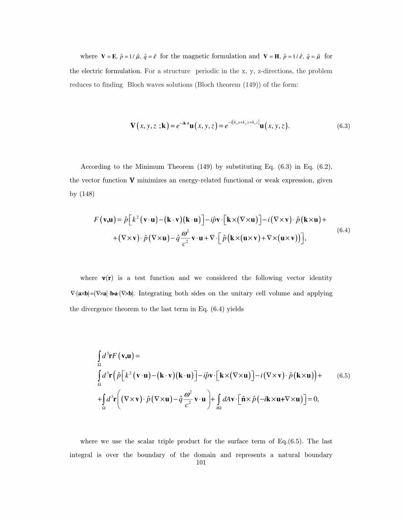
101

where ˆˆ ˆ ˆ, 1 / ,p qµ ε= = =V E for the magnetic formulation and ˆˆ ˆ ˆ, 1 / ,p qε µ= = =V H for

the electric formulation. For a structure periodic in the x, y, z-directions, the problem

reduces to finding Bloch waves solutions (Bloch theorem (149)) of the form:

( ) ( ) ( ) ( ), , ; , , , , .k rV k u ux y zi k x k y k zix y z e x y z e x y z

− + +− ⋅= = (6.3)

According to the Minimum Theorem (149) by substituting Eq. (6.3) in Eq. (6.2),

the vector function V V V V minimizes an energy-related functional or weak expression, given

by (148)

( ) ( ) ( )( ) ( ) ( ) ( )

( ) ( ) ( ) ( )( )

2

2

2

ˆ ˆ ˆ

ˆ ˆ ˆ ,

v,u v u k v k u v k u v k u

v u v u k u v u v

F p k ip i p

p q pc

ω

= ⋅ − ⋅ ⋅ − ⋅ × ∇× − ∇× ⋅ × +

+ ∇× ⋅ ∇× − ⋅ + ∇ ⋅ × × + ∇× ×

(6.4)

where vvvv(rrrr) is a test function and we considered the following vector identity

( ) ( ) ( ).∇⋅ × = ∇× ⋅ ⋅ ∇×a b a b-a b Integrating both sides on the unitary cell volume and applying

the divergence theorem to the last term in Eq. (6.4) yields

( )

( ) ( )( ) ( ) ( ) ( )( )

( ) ( ) ( )

3

3 2

23

2

ˆ ˆ ˆ

ˆˆ ˆ ˆ 0,

r v,u

r v u k v k u v k u v k u

r v u v u v n k u+ u

d F

d p k ip i p

d p q dA p ic

ω

Ω

Ω

Ω ∂Ω

=

⋅ − ⋅ ⋅ − ⋅ × ∇× − ∇× ⋅ × +

+ ∇× ⋅ ∇× − ⋅ + ⋅ × − × ∇× =

∫

∫

∫ ∫

(6.5)

where we use the scalar triple product for the surface term of Eq.(6.5). The last

integral is over the boundary of the domain and represents a natural boundary

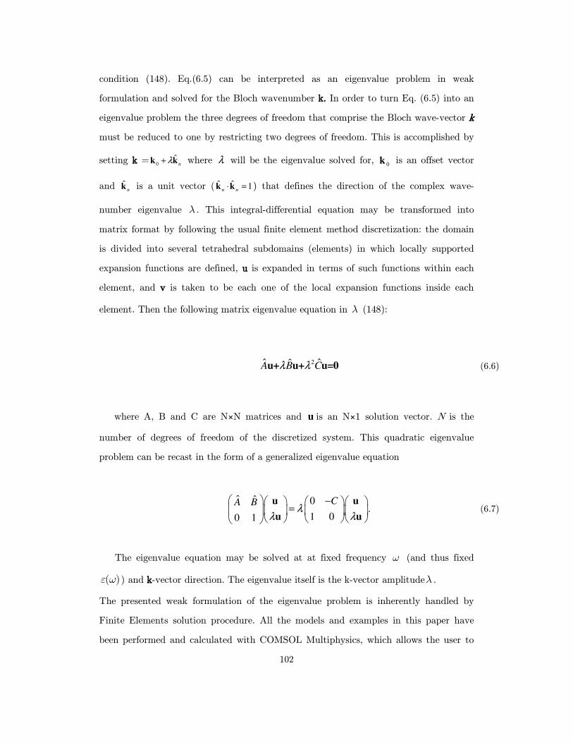
102

condition (148). Eq.(6.5) can be interpreted as an eigenvalue problem in weak

formulation and solved for the Bloch wavenumber k.k.k.k. In order to turn Eq. (6.5) into an

eigenvalue problem the three degrees of freedom that comprise the Bloch wave-vector k k k k

must be reduced to one by restricting two degrees of freedom. This is accomplished by

setting k k k k =0

ˆn

λ+k k where λ will be the eigenvalue solved for, 0k is an offset vector

and ˆn

k is a unit vector ( ˆ ˆ 1n n

⋅ =k k ) that defines the direction of the complex wave-

number eigenvalue λ . This integral-differential equation may be transformed into

matrix format by following the usual finite element method discretization: the domain

is divided into several tetrahedral subdomains (elements) in which locally supported

expansion functions are defined, uuuu is expanded in terms of such functions within each

element, and vvvv is taken to be each one of the local expansion functions inside each

element. Then the following matrix eigenvalue equation in λ (148):

2ˆ ˆˆu+ u+ u=0A B Cλ λ (6.6)

where A, B and C are N×N matrices and u is an N×1 solution vector. N is the

number of degrees of freedom of the discretized system. This quadratic eigenvalue

problem can be recast in the form of a generalized eigenvalue equation

ˆ ˆ 0

.1 00 1

u u

u u

CA Bλ

λ λ

− =

(6.7)

The eigenvalue equation may be solved at at fixed frequency ω (and thus fixed

( )ε ω ) and kkkk-vector direction. The eigenvalue itself is the k-vector amplitudeλ .

The presented weak formulation of the eigenvalue problem is inherently handled by

Finite Elements solution procedure. All the models and examples in this paper have

been performed and calculated with COMSOL Multiphysics, which allows the user to

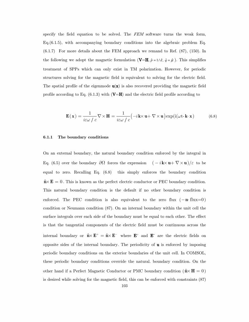
103

specify the field equation to be solved. The FEM software turns the weak form,

Eq.(6.1.5), with accompanying boundary conditions into the algebraic problem Eq.

(6.1.7) For more details about the FEM approach we remand to Ref. (87), (150). In

the following we adopt the magnetic formulation (VVVV=HHHH, ˆˆ ˆ ˆ1 / ,p qε µ= = ). This simplifies

treatment of SPPs which can only exist in TM polarization. However, for periodic

structures solving for the magnetic field is equivalent to solving for the electric field.

The spatial profile of the eigenmode uuuu(xxxx) is also recovered providing the magnetic field

profile according to Eq. (6.1.3) with (VVVV=HHHH) and the electric field profile according to

( )1 1

( ) exp(i( t- )ii c i c

ωεω εω

= ∇× = − × +∇× ⋅E x H k u u k x/ /

(6.8)

6.1.1 The boundary conditions

On an external boundary, the natural boundary condition enforced by the integral in

Eq. (6.5) over the boundary ∂Ω forces the expression ( )/i ε− × +∇×k u u to be

equal to zero. Recalling Eq. (6.8) this simply enforces the boundary condition

0× =n E . This is known as the perfect electric conductor or PEC boundary condition.

This natural boundary condition is the default if no other boundary condition is

enforced. The PEC condition is also equivalent to the zero flux ( flux=0− ⋅n )

condition or Neumann condition (87). On an internal boundary within the unit cell the

surface integrals over each side of the boundary must be equal to each other. The effect

is that the tangential components of the electric field must be continuous across the

internal boundary or + −× = ׈ ˆn E n E where EEEE+ and EEEE− are the electric fields on

opposite sides of the internal boundary. The periodicity of u u u u is enforced by imposing

periodic boundary conditions on the exterior boundaries of the unit cell. In COMSOL,

these periodic boundary conditions override the natural. boundary condition. On the

other hand if a Perfect Magnetic Conductor or PMC boundary condition ( 0× =n H )

is desired while solving for the magnetic field, this can be enforced with constraints (87)

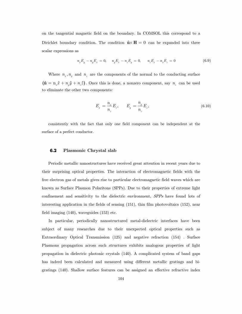
104

on the tangential magnetic field on the boundary. In COMSOL this correspond to a

Dirichlet boundary condition. The condition 0× =n H can be expanded into three

scalar expressions as

0, 0, 0x y y x y x z y z x x zn E n E n E n E n E n E− = − = − = (6.9)

Where xn ,

yn and

zn are the components of the normal to the conducting surface

nx y zx n y n z= + +ˆ ˆ ˆ ˆ(n ) . Once this is done, a nonzero component, say

zn can be used

to eliminate the other two components:

, , yx

x z y z

z z

nnE E E E

n n= = (6.10)

consistently with the fact that only one field component can be independent at the

surface of a perfect conductor.

6.26.26.26.2 Plasmonic Chrystal slab

Periodic metallic nanostructures have received great attention in recent years due to

their surprising optical properties. The interaction of electromagnetic fields with the

free electron gas of metals gives rise to particular electromagnetic field waves which are

known as Surface Plasmon Polaritons (SPPs). Due to their properties of extreme light

confinement and sensitivity to the dielectric environment, SPPs have found lots of

interesting application in the fields of sensing (151), thin film photovoltaics (152), near

field imaging (140), waveguides (153) etc.

In particular, periodically nanostructured metal-dielectric interfaces have been

subject of many researches due to their unexpected optical properties such as

Extraordinary Optical Transmission (125) and negative refraction (154) . Surface

Plasmons propagation across such structures exhibits analogous properties of light

propagation in dielectric photonic crystals (140). A complicated system of band gaps

has indeed been calculated and measured using different metallic gratings and bi-

gratings (140). Shallow surface features can be assigned an effective refractive index

105

describing their interaction with SPP, thus enabling a complete analogy with 2D

photonic crystals. The description of Plasmonic Bloch waves propagating in a

plasmonic crystal slabs, however, is a much more challenging task with respect to the

description of photonic Bloch waves in fully periodic dielectric systems.

The treatment of Photonic Crystal Slabs (PCS), however, requires proper handling of

not only truly bound modes but also of leaky modes. This term addresses eigen-modes

whose crystal momentum lies inside the light cone. In these cases the mode can couple

to waves propagating in the semi-infinite half space resulting in radiative losses (3).

Simulation of open space boundaries is a tricky task both for methods based on

discretization of real space (like Finite Elements and Finite Differences) as well as for

methods suited for fully periodic structures (like Plane Wave Expansion method). A

common approach introduces a fictitious periodicity in the direction normal to the slab

(Super-cell approach (155),(3)). The period is chosen sufficiently large in order to

decouple the bound modes of the slabs. However, the artificial periodicity produces

many spurious modes and moreover it perturbs the physical eigen-modes profile and it

requires much computational time (because of the large super-cell size necessary for

decoupling of modes). Plane Wave Expansion Method has been extended by Shi and

coworkers (145) including Perfectly Matched Layers (PMLs) which correctly absorbs

leakage radiation. These layers are characterized by a slowly space varying relative

permittivity and permeability, properly designed in order to minimize reflection of

plane waves impinging on them at arbitrary incidence. The method can deal with

photonic crystal slabs with arbitrarily dispersive materials but only in case of absence

of losses, excluding therefore the important class of plasmonic crystal slabs. Other

methods, based on FDTD can handle the lossy dispersive problem but are

computationally very expensive (156). To our knowledge, a complete and efficient

numerical treatment of metallic planar crystals still lacks.

In this paper we adopt the weak formulation of the Helmholtz’s eigenvalue

equation, which allows to solve the problem with wave vector as eigenvalue, adding

PMLs to correctly deal with leaky modes radiation. The method is compared to

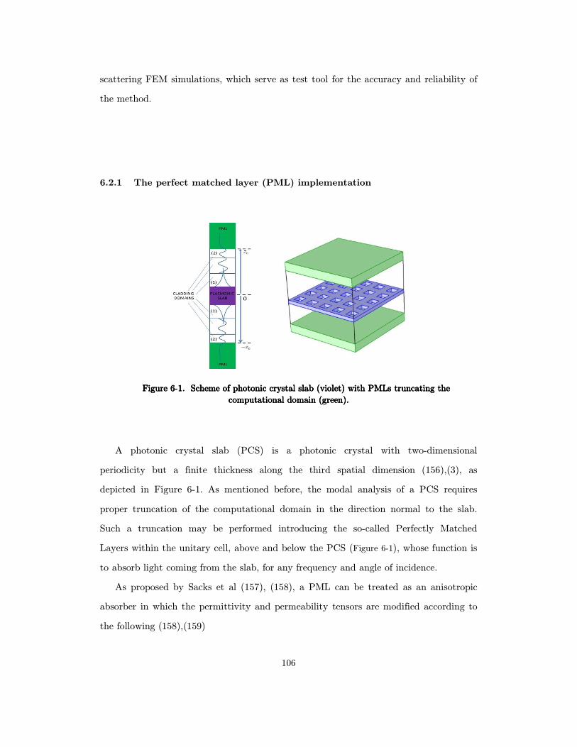
106

scattering FEM simulations, which serve as test tool for the accuracy and reliability of

the method.

6.2.1 The perfect matched layer (PML) implementation

Figure Figure Figure Figure 6666----1111. . . . Scheme of photonic crystal slab (violet) with PMLs truncating the Scheme of photonic crystal slab (violet) with PMLs truncating the Scheme of photonic crystal slab (violet) with PMLs truncating the Scheme of photonic crystal slab (violet) with PMLs truncating the

computational domain (green).computational domain (green).computational domain (green).computational domain (green).

A photonic crystal slab (PCS) is a photonic crystal with two-dimensional

periodicity but a finite thickness along the third spatial dimension (156),(3), as

depicted in Figure 6-1. As mentioned before, the modal analysis of a PCS requires

proper truncation of the computational domain in the direction normal to the slab.

Such a truncation may be performed introducing the so-called Perfectly Matched

Layers within the unitary cell, above and below the PCS (Figure 6-1), whose function is

to absorb light coming from the slab, for any frequency and angle of incidence.

As proposed by Sacks et al (157), (158), a PML can be treated as an anisotropic

absorber in which the permittivity and permeability tensors are modified according to

the following (158),(159)

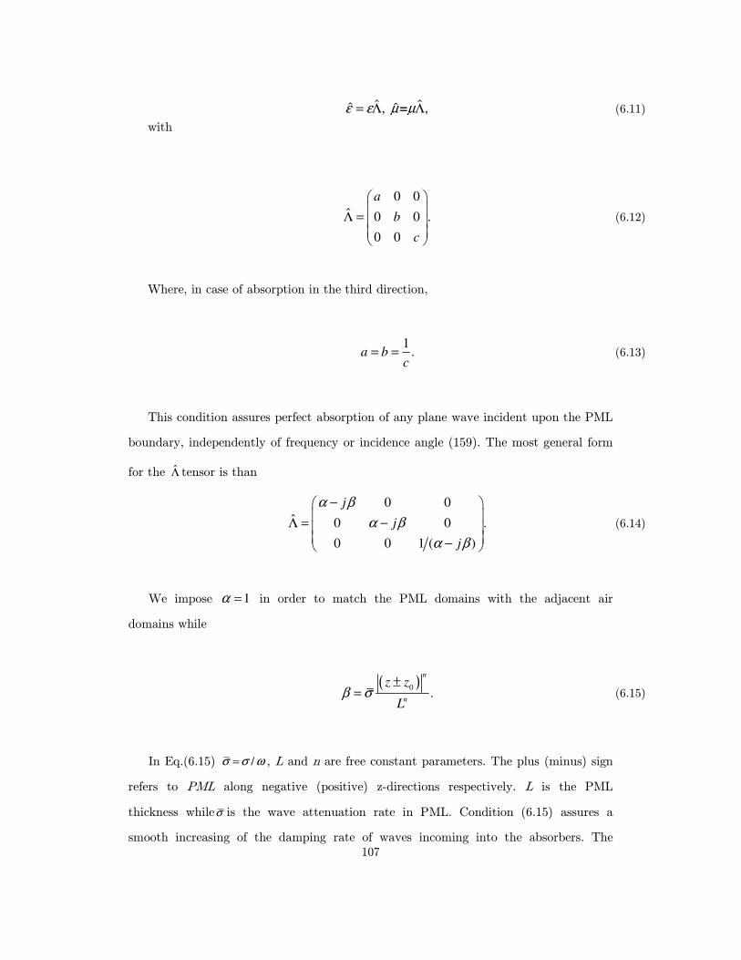
107

ˆ ˆˆ ˆ, , =ε ε µ µ= Λ Λ (6.11)

with

0 0

ˆ 0 0 .

0 0

a

b

c

Λ =

(6.12)

Where, in case of absorption in the third direction,

1

.a bc

= = (6.13)

This condition assures perfect absorption of any plane wave incident upon the PML

boundary, independently of frequency or incidence angle (159). The most general form

for the Λ tensor is than

0 0

ˆ 0 0 .

0 0 1 ( )

j

j

j

α β

α β

α β

−

Λ = − −

(6.14)

We impose 1α = in order to match the PML domains with the adjacent air

domains while

( )0

.

n

n

z z

Lβ σ

±= (6.15)

In Eq.(6.15) /σ σ ω= , L and n are free constant parameters. The plus (minus) sign

refers to PML along negative (positive) z-directions respectively. L is the PML

thickness whileσ is the wave attenuation rate in PML. Condition (6.15) assures a

smooth increasing of the damping rate of waves incoming into the absorbers. The

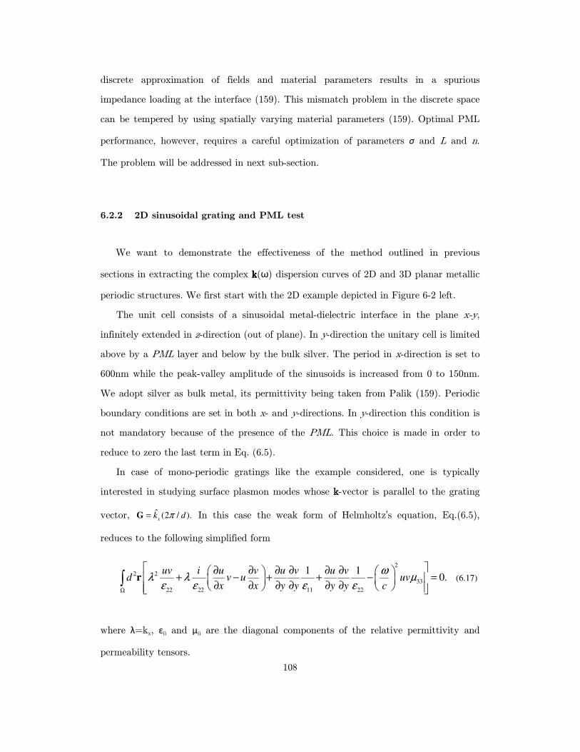
108

discrete approximation of fields and material parameters results in a spurious

impedance loading at the interface (159). This mismatch problem in the discrete space

can be tempered by using spatially varying material parameters (159). Optimal PML

performance, however, requires a careful optimization of parameters σ and L and n.

The problem will be addressed in next sub-section.

6.2.2 2D sinusoidal grating and PML test

We want to demonstrate the effectiveness of the method outlined in previous

sections in extracting the complex kkkk(ω) dispersion curves of 2D and 3D planar metallic

periodic structures. We first start with the 2D example depicted in Figure 6-2 left.

The unit cell consists of a sinusoidal metal-dielectric interface in the plane x-y,

infinitely extended in z-direction (out of plane). In y-direction the unitary cell is limited

above by a PML layer and below by the bulk silver. The period in x-direction is set to

600nm while the peak-valley amplitude of the sinusoids is increased from 0 to 150nm.

We adopt silver as bulk metal, its permittivity being taken from Palik (159). Periodic

boundary conditions are set in both x- and y-directions. In y-direction this condition is

not mandatory because of the presence of the PML. This choice is made in order to

reduce to zero the last term in Eq. (6.5).

In case of mono-periodic gratings like the example considered, one is typically

interested in studying surface plasmon modes whose kkkk-vector is parallel to the grating

vector, ˆ (2 / ).x

k dπ=G In this case the weak form of Helmholtz’s equation, Eq.(6.5),

reduces to the following simplified form

2

2 2

33

22 22 11 22

1 10.r

uv i u v u v u vd v u uv

x x y y y y c

ωλ λ µ

ε ε ε εΩ

∂ ∂ ∂ ∂ ∂ ∂ + − + + − =

∂ ∂ ∂ ∂ ∂ ∂ ∫ (6.17)

where λ=kx, εii and μii are the diagonal components of the relative permittivity and

permeability tensors.

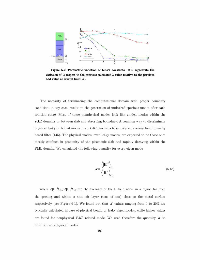
109

Figure Figure Figure Figure 6666----2222. Parametric variation of tensor constants. . Parametric variation of tensor constants. . Parametric variation of tensor constants. . Parametric variation of tensor constants. λ∆ representrepresentrepresentrepresentssss the the the the

variation of variation of variation of variation of λ respect to the previous respect to the previous respect to the previous respect to the previous calculated calculated calculated calculated λ value relative to the previous value relative to the previous value relative to the previous value relative to the previous

L/d value at several fixed L/d value at several fixed L/d value at several fixed L/d value at several fixed σ ....

The necessity of terminating the computational domain with proper boundary

condition, in any case, results in the generation of undesired spurious modes after each

solution stage. Most of these nonphysical modes look like guided modes within the

PML domains or between slab and absorbing boundary. A common way to discriminate

physical leaky or bound modes from PML modes is to employ an average field intensity

based filter (145). The physical modes, even leaky modes, are expected to be those ones

mostly confined in proximity of the plasmonic slab and rapidly decaying within the

PML domain. We calculated the following quantity for every eigen-mode

2

(1)

2

(2)

H

Hκ = (6.18)

where <|H|2>(1), <|H|

2>(2) are the averages of the H H H H field norm in a region far from

the grating and within a thin air layer (tens of nm) close to the metal surface

respectively (see Figure 6-1). We found out that κ values ranging from 0 to 20% are

typically calculated in case of physical bound or leaky eigen-modes, while higher values

are found for nonphysical PML–related mode. We used therefore the quantity κ to

filter out non-physical modes.

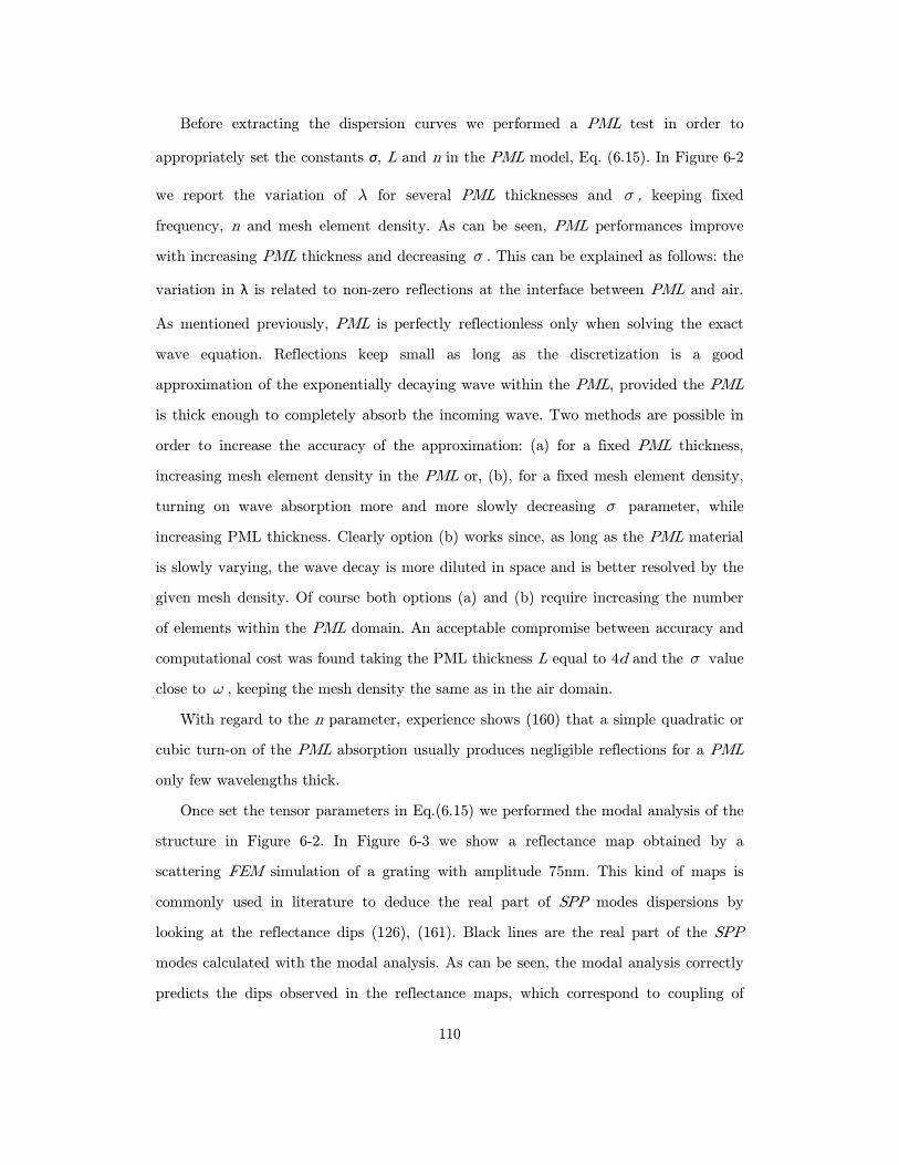
110

Before extracting the dispersion curves we performed a PML test in order to

appropriately set the constants σ, L and n in the PML model, Eq. (6.15). In Figure 6-2

we report the variation of λ for several PML thicknesses and σ , keeping fixed

frequency, n and mesh element density. As can be seen, PML performances improve

with increasing PML thickness and decreasing σ . This can be explained as follows: the

variation in λ is related to non-zero reflections at the interface between PML and air.

As mentioned previously, PML is perfectly reflectionless only when solving the exact

wave equation. Reflections keep small as long as the discretization is a good

approximation of the exponentially decaying wave within the PML, provided the PML

is thick enough to completely absorb the incoming wave. Two methods are possible in

order to increase the accuracy of the approximation: (a) for a fixed PML thickness,

increasing mesh element density in the PML or, (b), for a fixed mesh element density,

turning on wave absorption more and more slowly decreasing σ parameter, while

increasing PML thickness. Clearly option (b) works since, as long as the PML material

is slowly varying, the wave decay is more diluted in space and is better resolved by the

given mesh density. Of course both options (a) and (b) require increasing the number

of elements within the PML domain. An acceptable compromise between accuracy and

computational cost was found taking the PML thickness L equal to 4d and the σ value

close to ω , keeping the mesh density the same as in the air domain.

With regard to the n parameter, experience shows (160) that a simple quadratic or

cubic turn-on of the PML absorption usually produces negligible reflections for a PML

only few wavelengths thick.

Once set the tensor parameters in Eq.(6.15) we performed the modal analysis of the

structure in Figure 6-2. In Figure 6-3 we show a reflectance map obtained by a

scattering FEM simulation of a grating with amplitude 75nm. This kind of maps is

commonly used in literature to deduce the real part of SPP modes dispersions by

looking at the reflectance dips (126), (161). Black lines are the real part of the SPP

modes calculated with the modal analysis. As can be seen, the modal analysis correctly

predicts the dips observed in the reflectance maps, which correspond to coupling of

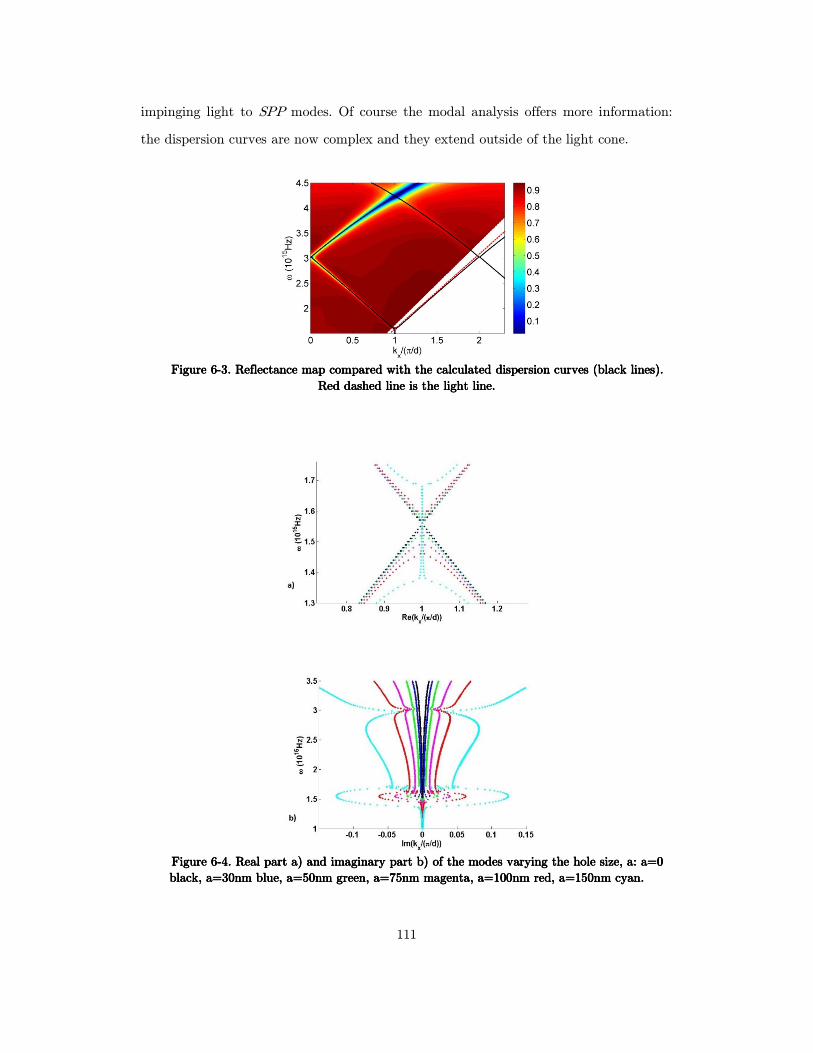
111

impinging light to SPP modes. Of course the modal analysis offers more information:

the dispersion curves are now complex and they extend outside of the light cone.

Figure Figure Figure Figure 6666----3333. Reflectance map compared with the calculated dispersion curves (black lines). . Reflectance map compared with the calculated dispersion curves (black lines). . Reflectance map compared with the calculated dispersion curves (black lines). . Reflectance map compared with the calculated dispersion curves (black lines).

Red dashed line is the light Red dashed line is the light Red dashed line is the light Red dashed line is the light linelinelineline....

Figure Figure Figure Figure 6666----4444. Real part a) and imaginary part b) of the modes. Real part a) and imaginary part b) of the modes. Real part a) and imaginary part b) of the modes. Real part a) and imaginary part b) of the modes varying the hole size, a: a=0 varying the hole size, a: a=0 varying the hole size, a: a=0 varying the hole size, a: a=0

black, a=30nm blue, a=50nm green, a=75nm magenta, a=100nm red, a=150nm cyan.black, a=30nm blue, a=50nm green, a=75nm magenta, a=100nm red, a=150nm cyan.black, a=30nm blue, a=50nm green, a=75nm magenta, a=100nm red, a=150nm cyan.black, a=30nm blue, a=50nm green, a=75nm magenta, a=100nm red, a=150nm cyan.

112

In Figure 5a it is reported real part of mode dispersion at the edge of first Brillouin

zone for increasing grating amplitudes. As well-known (126), the flat metal interface

sustains a SPP wave whose dispersion is given by 1/2

, 0( / ( ))

SPP F m d m dk k ε ε ε ε= + . When a

shallow periodic perturbation is introduced the mode dispersion remains close to the

flat case dispersion. The only remarkable difference with respect to the flat case is seen

at the edge of first Brillouin zone, where an energy gap is rapidly established with

increasing grating depth (162). In general, energy gaps occur at the crossing points of

the flat metal inferface SPP dispersion curves, i.e. at the edge and at the center of first

Brillouin zone (kx =π /d and kx=0 respectively). When ω increases, starting from

zero, the first crossover defines the so-called first order stop band (162), which

corresponds to the coupling of two counter-propagating surface waves. As discussed in

Ref. (162) for the case of lossless metal gratings, if a surface mode propagates on a

corrugated surface whose grating wave vector G=2π /d is twice the mode wave vector,

this results in the formation of a standing wave pattern. For symmetry reasons, the

mode field distribution on the surface may then take only two alternative

configurations, having different energies. The two standing wave patterns take different

positions with respect to the peaks and troughs of the grating. The low frequency

solution concentrate its energy around the grating peaks (high effective permittivity

region) while the high frequency solution concentrate its energy in the troughs of the

grating (low effective permittivity region). This situation is analogue to the band gap

formation in case of 1D photonic crystals (3). It is worth noting in Figure 6-4a that the

modal method converges to a solution also at frequencies within the band gap. In

particular the band, at frequencies close to the lower gap edge, rises steeply through a

continuum of states toward the upper gap edge, reaching the value kx=π /d only in one

point. The gap edges are actually not well defined, especially for higher amplitude

gratings. This behavior was already noticed in similar modal analyses performed with

real frequency and complex Bloch wave vector. The frequency gap however is more

evident looking at the imaginary part of the mode dispersions (Figure 6-4b). At

frequencies corresponding to the energy gap the imaginary part assumes great values,

reaching a maximum at the centre of the gap. The phenomenon becomes more evident

113

with increasing grating depths, as expected. The mode in this frequency range has a

great dissipation which prevents it to propagate in the groove direction, thus it is

sometimes referred as gap-like mode

For frequencies above the upper gap edge (ω > 1.7x1015Hz) the imaginary part of

the Bloch wave vector has values much greater than for frequencies below the gap. This

is because the folded plasmonic band enters the light cone and radiative copling to

propagating waves in the upper air half space becomes possible. In Figure 6-5 we show

the z-component of the eigen-mode magnetic field at a frequency of ω = 2.5x1015Hz for

grating amplitudes of 0, 30 and 100nm. In the flat case, the mode is a guided eigen-

mode of the metal-dielectric interface and is perfectly confined (Figure 6-5a). As

already pointed out, for small grating depths, the SPP wave vector is only slightly

perturbed with respect to kSPP,F. In this situation the mode remains well confined as in

the flat case and the main damping is due to losses in metal (see Figure 6-5b). The

mode confinement decreases with increasing the grating amplitude, and stronger

leakage radiation is observed (see Figure 6-5c). It is worth noting how the leakage

radiation is perfectly exponentially decaying when crossing the PML domain (see Figure

6-5d) with almost zero spurious back reflections.

Figure Figure Figure Figure 6666----5555. From left to right: z. From left to right: z. From left to right: z. From left to right: z----component of the component of the component of the component of the

magnetic field (in a. u.) for magnetic field (in a. u.) for magnetic field (in a. u.) for magnetic field (in a. u.) for aaaa=0 (a), =0 (a), =0 (a), =0 (a), aaaa=30nm (b), =30nm (b), =30nm (b), =30nm (b),

aaaa=100nm (c), z=100nm (c), z=100nm (c), z=100nm (c), z----component of the magnetic field (in a. u.) component of the magnetic field (in a. u.) component of the magnetic field (in a. u.) component of the magnetic field (in a. u.)

inside the cladding region (under the black horizontal inside the cladding region (under the black horizontal inside the cladding region (under the black horizontal inside the cladding region (under the black horizontal

line) and the PML domain (above the black horizontal line) and the PML domain (above the black horizontal line) and the PML domain (above the black horizontal line) and the PML domain (above the black horizontal

line) (d).line) (d).line) (d).line) (d).

At ω ≅ 3x1015Hz a second crossover of the dispersion curves occurs (see Figure 6-3).

This point has been subject of several discussions both in metallic and dielectric

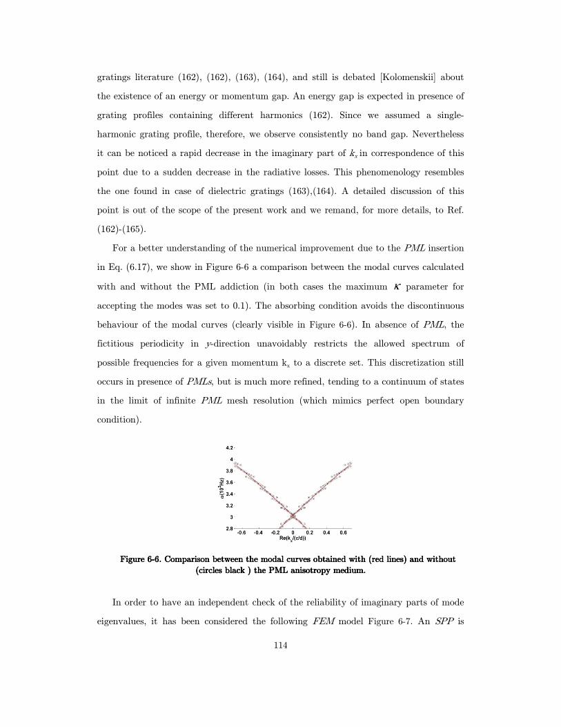
114

gratings literature (162), (162), (163), (164), and still is debated [Kolomenskii] about

the existence of an energy or momentum gap. An energy gap is expected in presence of

grating profiles containing different harmonics (162). Since we assumed a single-

harmonic grating profile, therefore, we observe consistently no band gap. Nevertheless

it can be noticed a rapid decrease in the imaginary part of kx in correspondence of this

point due to a sudden decrease in the radiative losses. This phenomenology resembles

the one found in case of dielectric gratings (163),(164). A detailed discussion of this

point is out of the scope of the present work and we remand, for more details, to Ref.

(162)-(165).

For a better understanding of the numerical improvement due to the PML insertion

in Eq. (6.17), we show in Figure 6-6 a comparison between the modal curves calculated

with and without the PML addiction (in both cases the maximum κ parameter for

accepting the modes was set to 0.1). The absorbing condition avoids the discontinuous

behaviour of the modal curves (clearly visible in Figure 6-6). In absence of PML, the

fictitious periodicity in y-direction unavoidably restricts the allowed spectrum of

possible frequencies for a given momentum kx to a discrete set. This discretization still

occurs in presence of PMLs, but is much more refined, tending to a continuum of states

in the limit of infinite PML mesh resolution (which mimics perfect open boundary

condition).

Figure Figure Figure Figure 6666----6666. Comparison between the modal curves obtained with (red lines) and without . Comparison between the modal curves obtained with (red lines) and without . Comparison between the modal curves obtained with (red lines) and without . Comparison between the modal curves obtained with (red lines) and without

(circles black ) (circles black ) (circles black ) (circles black ) the PML anisotropy medium.the PML anisotropy medium.the PML anisotropy medium.the PML anisotropy medium.

In order to have an independent check of the reliability of imaginary parts of mode

eigenvalues, it has been considered the following FEM model Figure 6-7. An SPP is

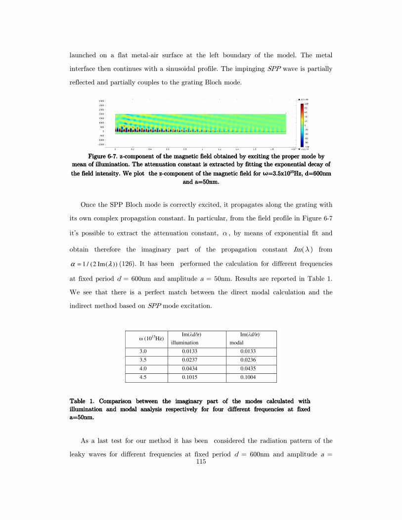
115

launched on a flat metal-air surface at the left boundary of the model. The metal

interface then continues with a sinusoidal profile. The impinging SPP wave is partially

reflected and partially couples to the grating Bloch mode.

Figure Figure Figure Figure 6666----7777. z. z. z. z----component of the magnetic field obtained by exciting the proper mode by component of the magnetic field obtained by exciting the proper mode by component of the magnetic field obtained by exciting the proper mode by component of the magnetic field obtained by exciting the proper mode by

mean of illumination. The attenuation constant is extracted by fittingmean of illumination. The attenuation constant is extracted by fittingmean of illumination. The attenuation constant is extracted by fittingmean of illumination. The attenuation constant is extracted by fitting the exponential decay of the exponential decay of the exponential decay of the exponential decay of

the field intensity. We plot the zthe field intensity. We plot the zthe field intensity. We plot the zthe field intensity. We plot the z----component of the magnetic field for component of the magnetic field for component of the magnetic field for component of the magnetic field for ω=3.5x10=3.5x10=3.5x10=3.5x1015151515Hz, d=600nm Hz, d=600nm Hz, d=600nm Hz, d=600nm

and a=50nm.and a=50nm.and a=50nm.and a=50nm.

Once the SPP Bloch mode is correctly excited, it propagates along the grating with

its own complex propagation constant. In particular, from the field profile in Figure 6-7

it’s possible to extract the attenuation constant, α , by means of exponential fit and

obtain therefore the imaginary part of the propagation constant Im(λ ) from

1 / (2 Im( ))α λ= (126). It has been performed the calculation for different frequencies

at fixed period d = 600nm and amplitude a = 50nm. Results are reported in Table 1.

We see that there is a perfect match between the direct modal calculation and the

indirect method based on SPP mode excitation.

ω (1015Hz) Im(λd/π)

illumination

Im(λd/π)

modal

3.0 0.0133 0.0133

3.5 0.0237 0.0236

4.0 0.0434 0.0435

4.5 0.1015 0.1004

Table 1. Comparison between the imaginary part of the modes calculated with Table 1. Comparison between the imaginary part of the modes calculated with Table 1. Comparison between the imaginary part of the modes calculated with Table 1. Comparison between the imaginary part of the modes calculated with

illumination and illumination and illumination and illumination and modal analysis respectively for four different frequencies at fixed modal analysis respectively for four different frequencies at fixed modal analysis respectively for four different frequencies at fixed modal analysis respectively for four different frequencies at fixed

a=50nm.a=50nm.a=50nm.a=50nm.

As a last test for our method it has been considered the radiation pattern of the

leaky waves for different frequencies at fixed period d = 600nm and amplitude a =

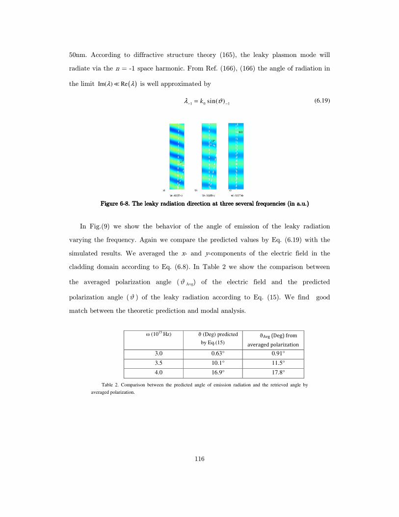
116

50nm. According to diffractive structure theory (165), the leaky plasmon mode will

radiate via the n = -1 space harmonic. From Ref. (166), (166) the angle of radiation in

the limit ( )Im( ) Reλ λ≪ is well approximated by

1 0 1sin( )kλ ϑ− −= (6.19)

Figure Figure Figure Figure 6666----8888. The leaky radiation direction at three several frequencies (in a.u.). The leaky radiation direction at three several frequencies (in a.u.). The leaky radiation direction at three several frequencies (in a.u.). The leaky radiation direction at three several frequencies (in a.u.)

In Fig.(9) we show the behavior of the angle of emission of the leaky radiation

varying the frequency. Again we compare the predicted values by Eq. (6.19) with the

simulated results. We averaged the x- and y-components of the electric field in the

cladding domain according to Eq. (6.8). In Table 2 we show the comparison between

the averaged polarization angle (ϑ Avg) of the electric field and the predicted

polarization angle (ϑ ) of the leaky radiation according to Eq. (15). We find good

match between the theoretic prediction and modal analysis.

ω (1015 Hz) ϑ (Deg) predicted

by Eq.(15)

ϑAvg (Deg) from

averaged polarization

3.0 0.63° 0.91°

3.5 10.1° 11.5°

4.0 16.9° 17.8°

Table 2. Comparison between the predicted angle of emission radiation and the retrieved angle by

averaged polarization.

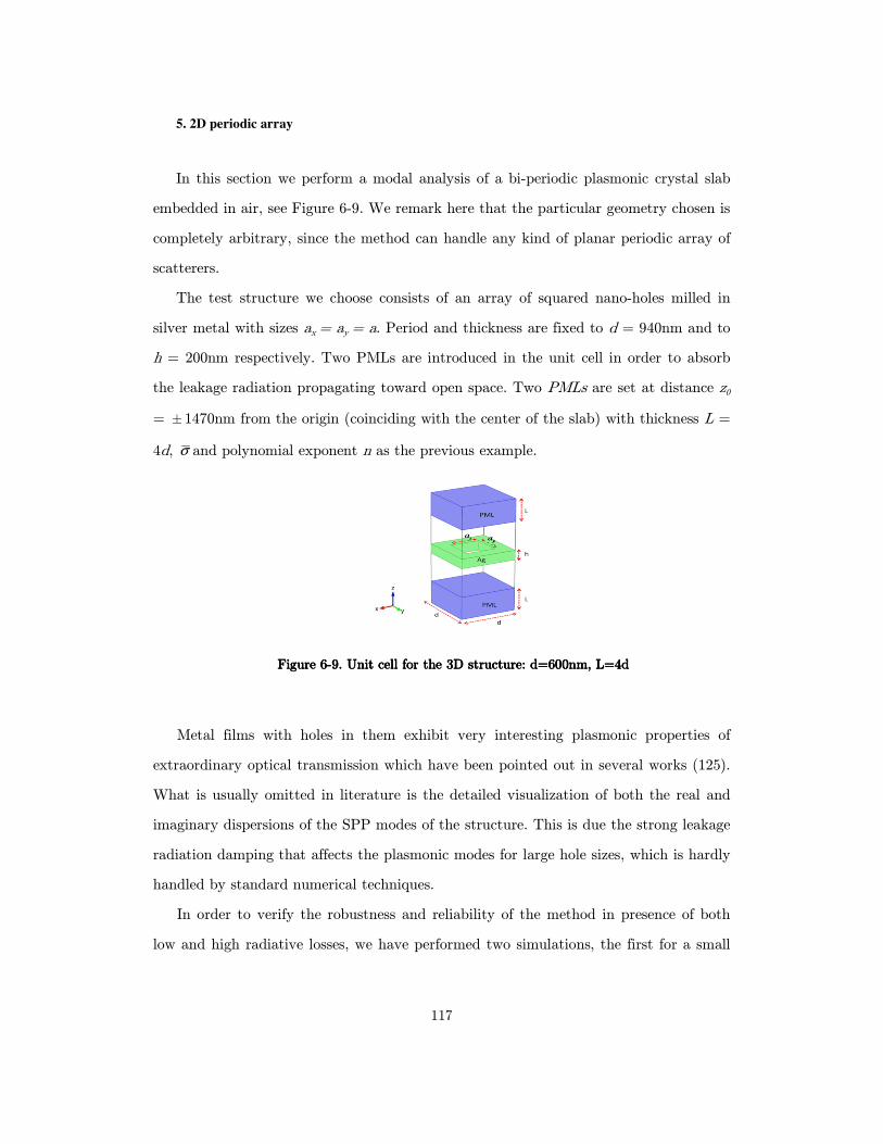
117

5. 2D periodic array

In this section we perform a modal analysis of a bi-periodic plasmonic crystal slab

embedded in air, see Figure 6-9. We remark here that the particular geometry chosen is

completely arbitrary, since the method can handle any kind of planar periodic array of

scatterers.

The test structure we choose consists of an array of squared nano-holes milled in

silver metal with sizes ax = ay = a. Period and thickness are fixed to d = 940nm and to

h = 200nm respectively. Two PMLs are introduced in the unit cell in order to absorb

the leakage radiation propagating toward open space. Two PMLs are set at distance z0

= ± 1470nm from the origin (coinciding with the center of the slab) with thickness L =

4d, σ and polynomial exponent n as the previous example.

Figure Figure Figure Figure 6666----9999. Unit cell for . Unit cell for . Unit cell for . Unit cell for the 3D structure: d=600nm, L=4dthe 3D structure: d=600nm, L=4dthe 3D structure: d=600nm, L=4dthe 3D structure: d=600nm, L=4d

Metal films with holes in them exhibit very interesting plasmonic properties of

extraordinary optical transmission which have been pointed out in several works (125).

What is usually omitted in literature is the detailed visualization of both the real and

imaginary dispersions of the SPP modes of the structure. This is due the strong leakage

radiation damping that affects the plasmonic modes for large hole sizes, which is hardly

handled by standard numerical techniques.

In order to verify the robustness and reliability of the method in presence of both

low and high radiative losses, we have performed two simulations, the first for a small

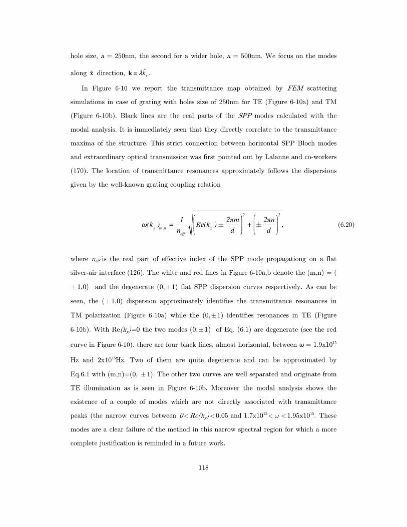
118

hole size, a = 250nm, the second for a wider hole, a = 500nm. We focus on the modes

along x direction, ˆx

kλk = .

In Figure 6-10 we report the transmittance map obtained by FEM scattering

simulations in case of grating with holes size of 250nm for TE (Figure 6-10a) and TM

(Figure 6-10b). Black lines are the real parts of the SPP modes calculated with the

modal analysis. It is immediately seen that they directly correlate to the transmittance

maxima of the structure. This strict connection between horizontal SPP Bloch modes

and extraordinary optical transmission was first pointed out by Lalanne and co-workers

(170). The location of transmittance resonances approximately follows the dispersions

given by the well-known grating coupling relation

,

,m n

± ±

2 2

x x

eff

1 2πm 2πnω(k ) = Re(k ) +

n d d (6.20)

where neff is the real part of effective index of the SPP mode propagationg on a flat

silver-air interface (126). The white and red lines in Figure 6-10a,b denote the (m,n) = (

±1,0) and the degenerate (0,± 1) flat SPP dispersion curves respectively. As can be

seen, the (±1,0) dispersion approximately identifies the transmittance resonances in

TM polarization (Figure 6-10a) while the (0,±1) identifies resonances in TE (Figure

6-10b). With Re(ky)=0 the two modes (0,±1) of Eq. (6.1) are degenerate (see the red

curve in Figure 6-10). there are four black lines, almost horizontal, between ω = 1.9x1015

Hz and 2x1015Hz. Two of them are quite degenerate and can be approximated by

Eq.6.1 with (m,n)=(0, ± 1). The other two curves are well separated and originate from

TE illumination as is seen in Figure 6-10b. Moreover the modal analysis shows the

existence of a couple of modes which are not directly associated with transmittance

peaks (the narrow curves between 0<Re(ky)< 0.05 and 1.7x1015 ω< < 1.95x1015. These

modes are a clear failure of the method in this narrow spectral region for which a more

complete justification is reminded in a future work.

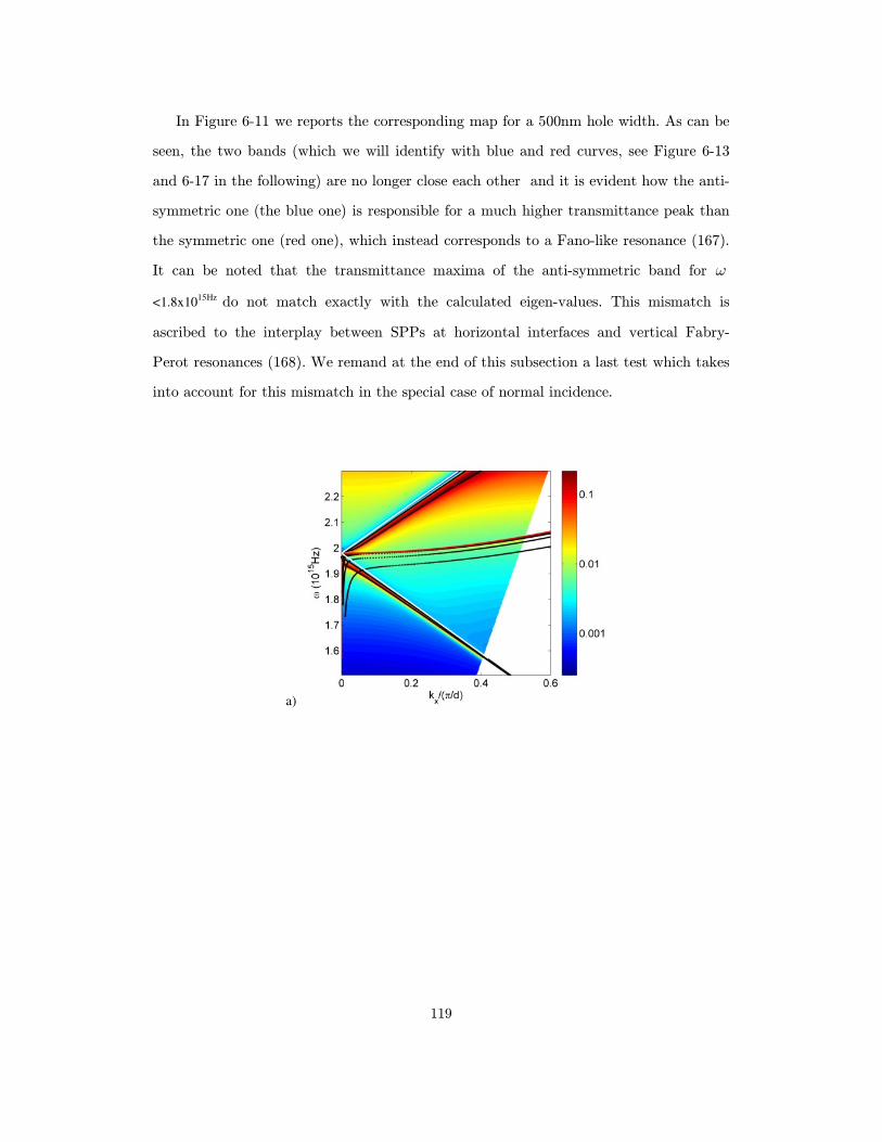
119

In Figure 6-11 we reports the corresponding map for a 500nm hole width. As can be

seen, the two bands (which we will identify with blue and red curves, see Figure 6-13

and 6-17 in the following) are no longer close each other and it is evident how the anti-

symmetric one (the blue one) is responsible for a much higher transmittance peak than

the symmetric one (red one), which instead corresponds to a Fano-like resonance (167).

It can be noted that the transmittance maxima of the anti-symmetric band for ω

<1.8x1015Hz do not match exactly with the calculated eigen-values. This mismatch is

ascribed to the interplay between SPPs at horizontal interfaces and vertical Fabry-

Perot resonances (168). We remand at the end of this subsection a last test which takes

into account for this mismatch in the special case of normal incidence.

a)

120

b)

Figure Figure Figure Figure 6666----10101010. Transmittance map . Transmittance map . Transmittance map . Transmittance map for TM (a),TE (b) ,propagation for TM (a),TE (b) ,propagation for TM (a),TE (b) ,propagation for TM (a),TE (b) ,propagation compared with the compared with the compared with the compared with the

calculated dispersion curves (black lines) calculated dispersion curves (black lines) calculated dispersion curves (black lines) calculated dispersion curves (black lines) and the grating dispersion curves of modes (1,0) , and the grating dispersion curves of modes (1,0) , and the grating dispersion curves of modes (1,0) , and the grating dispersion curves of modes (1,0) ,

(white line) and the degenerate mode (0,(white line) and the degenerate mode (0,(white line) and the degenerate mode (0,(white line) and the degenerate mode (0,± 1),(red line) 1),(red line) 1),(red line) 1),(red line) for a=250nm for a=250nm for a=250nm for a=250nm ....

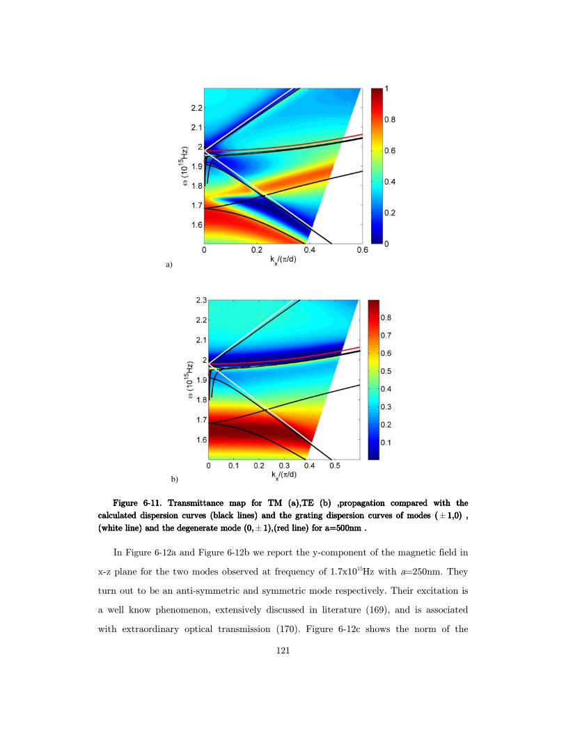
121

a)

b)

Figure Figure Figure Figure 6666----11111111.... Transmittance map Transmittance map Transmittance map Transmittance map for TM (a),TE (b) ,propagation for TM (a),TE (b) ,propagation for TM (a),TE (b) ,propagation for TM (a),TE (b) ,propagation compared with the compared with the compared with the compared with the

calculated dispersion curves (black lines) calculated dispersion curves (black lines) calculated dispersion curves (black lines) calculated dispersion curves (black lines) and the grating dispersion curves of modes (and the grating dispersion curves of modes (and the grating dispersion curves of modes (and the grating dispersion curves of modes (± 1,0) , 1,0) , 1,0) , 1,0) ,

(white line) and the degenerate mode (0,(white line) and the degenerate mode (0,(white line) and the degenerate mode (0,(white line) and the degenerate mode (0,± 1),(red line) for a=5001),(red line) for a=5001),(red line) for a=5001),(red line) for a=500nm nm nm nm ....

In Figure 6-12a and Figure 6-12b we report the y-component of the magnetic field in

x-z plane for the two modes observed at frequency of 1.7x1015Hz with a=250nm. They

turn out to be an anti-symmetric and symmetric mode respectively. Their excitation is

a well know phenomenon, extensively discussed in literature (169), and is associated

with extraordinary optical transmission (170). Figure 6-12c shows the norm of the

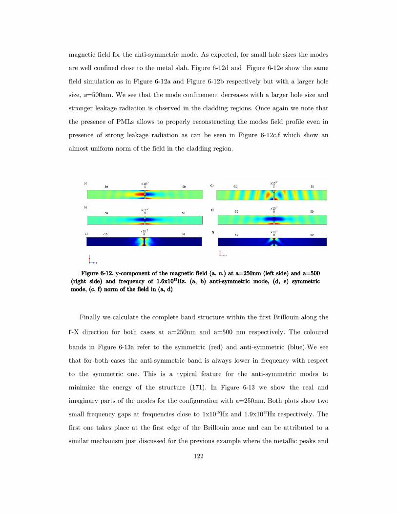
122

magnetic field for the anti-symmetric mode. As expected, for small hole sizes the modes

are well confined close to the metal slab. Figure 6-12d and Figure 6-12e show the same

field simulation as in Figure 6-12a and Figure 6-12b respectively but with a larger hole

size, a=500nm. We see that the mode confinement decreases with a larger hole size and

stronger leakage radiation is observed in the cladding regions. Once again we note that

the presence of PMLs allows to properly reconstructing the modes field profile even in

presence of strong leakage radiation as can be seen in Figure 6-12c,f which show an

almost uniform norm of the field in the cladding region.

Figure Figure Figure Figure 6666----12121212. . . . yyyy----component of the magnetic field (a. u.) at a=250nm component of the magnetic field (a. u.) at a=250nm component of the magnetic field (a. u.) at a=250nm component of the magnetic field (a. u.) at a=250nm (left side) and a=500 (left side) and a=500 (left side) and a=500 (left side) and a=500

(right side) and frequency of 1.6x10(right side) and frequency of 1.6x10(right side) and frequency of 1.6x10(right side) and frequency of 1.6x1015151515Hz. (a, b) antiHz. (a, b) antiHz. (a, b) antiHz. (a, b) anti----symmetric mode, (d, e) symmetric symmetric mode, (d, e) symmetric symmetric mode, (d, e) symmetric symmetric mode, (d, e) symmetric

mode, (c, f) norm of the field in (a, d)mode, (c, f) norm of the field in (a, d)mode, (c, f) norm of the field in (a, d)mode, (c, f) norm of the field in (a, d)

Finally we calculate the complete band structure within the first Brillouin along the

Г-X direction for both cases at a=250nm and a=500 nm respectively. The coloured

bands in Figure 6-13a refer to the symmetric (red) and anti-symmetric (blue).We see

that for both cases the anti-symmetric band is always lower in frequency with respect

to the symmetric one. This is a typical feature for the anti-symmetric modes to

minimize the energy of the structure (171). In Figure 6-13 we show the real and

imaginary parts of the modes for the configuration with a=250nm. Both plots show two

small frequency gaps at frequencies close to 1x1015Hz and 1.9x1015Hz respectively. The

first one takes place at the first edge of the Brillouin zone and can be attributed to a

similar mechanism just discussed for the previous example where the metallic peaks and

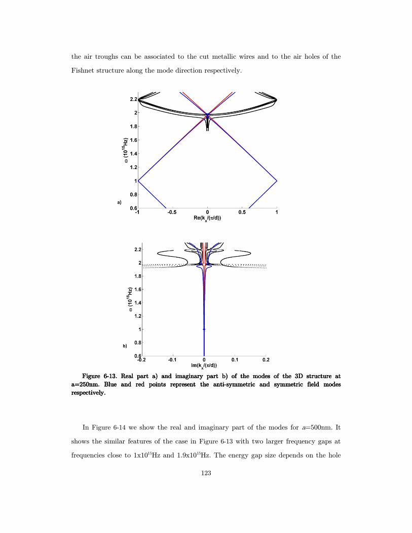
123

the air troughs can be associated to the cut metallic wires and to the air holes of the

Fishnet structure along the mode direction respectively.

Figure Figure Figure Figure 6666----13131313. Real part a) and imaginary part b) of the modes of the 3D structure at . Real part a) and imaginary part b) of the modes of the 3D structure at . Real part a) and imaginary part b) of the modes of the 3D structure at . Real part a) and imaginary part b) of the modes of the 3D structure at

a=250nm. Blue and red points represent the a=250nm. Blue and red points represent the a=250nm. Blue and red points represent the a=250nm. Blue and red points represent the antiantiantianti----symmetric and symmetric field modes symmetric and symmetric field modes symmetric and symmetric field modes symmetric and symmetric field modes

respectively.respectively.respectively.respectively.

In Figure 6-14 we show the real and imaginary part of the modes for a=500nm. It

shows the similar features of the case in Figure 6-13 with two larger frequency gaps at

frequencies close to 1x1015Hz and 1.9x1015Hz. The energy gap size depends on the hole

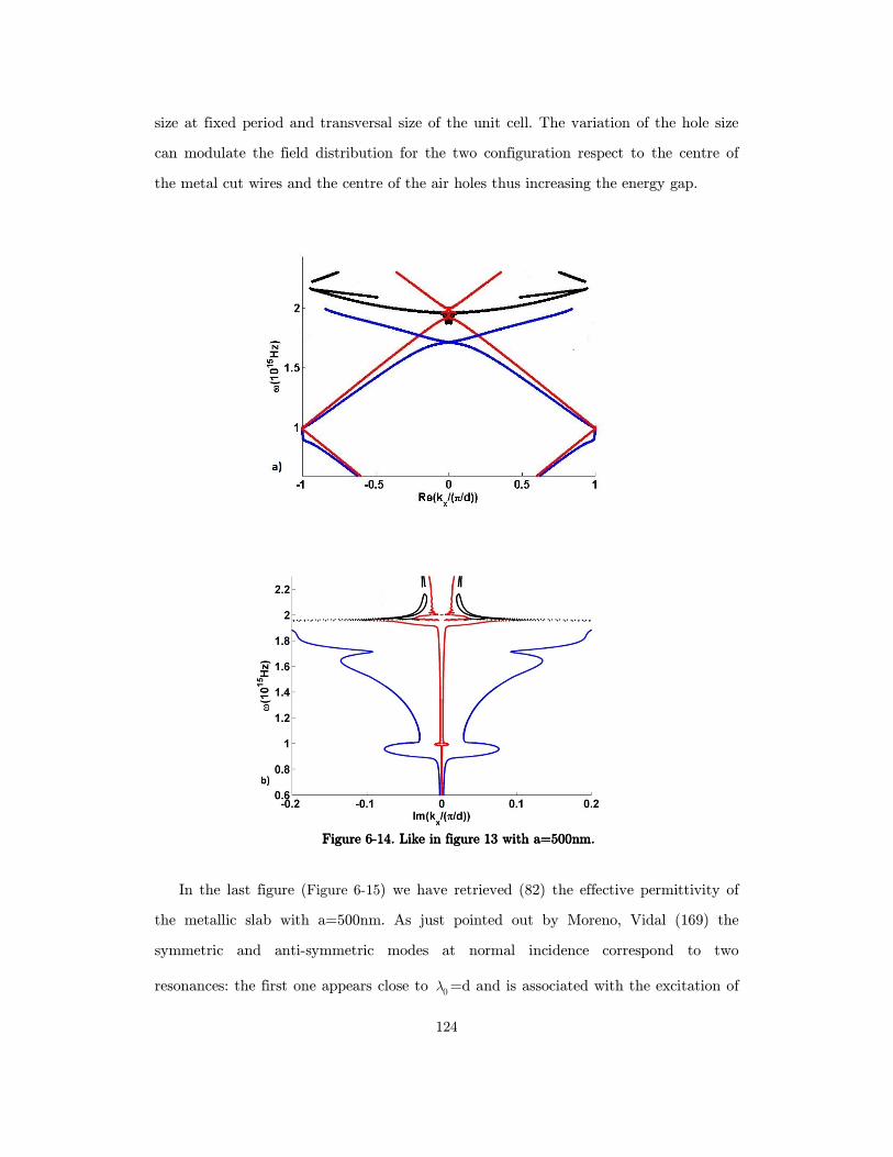
124

size at fixed period and transversal size of the unit cell. The variation of the hole size

can modulate the field distribution for the two configuration respect to the centre of

the metal cut wires and the centre of the air holes thus increasing the energy gap.

Figure Figure Figure Figure 6666----14141414. Like in figure 13 with a=500nm.. Like in figure 13 with a=500nm.. Like in figure 13 with a=500nm.. Like in figure 13 with a=500nm.

In the last figure (Figure 6-15) we have retrieved (82) the effective permittivity of

the metallic slab with a=500nm. As just pointed out by Moreno, Vidal (169) the

symmetric and anti-symmetric modes at normal incidence correspond to two

resonances: the first one appears close to 0λ =d and is associated with the excitation of

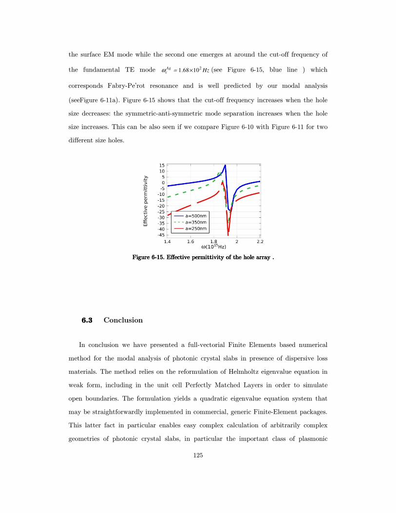
125

the surface EM mode while the second one emerges at around the cut-off frequency of

the fundamental TE mode 21.68 10

Agc Hzω ×≃ (see Figure 6-15, blue line ) which

corresponds Fabry-Pe’rot resonance and is well predicted by our modal analysis

(seeFigure 6-11a). Figure 6-15 shows that the cut-off frequency increases when the hole

size decreases: the symmetric-anti-symmetric mode separation increases when the hole

size increases. This can be also seen if we compare Figure 6-10 with Figure 6-11 for two

different size holes.

Figure Figure Figure Figure 6666----15151515. Effective permittivity of the hole array .. Effective permittivity of the hole array .. Effective permittivity of the hole array .. Effective permittivity of the hole array .

6.36.36.36.3 Conclusion

In conclusion we have presented a full-vectorial Finite Elements based numerical

method for the modal analysis of photonic crystal slabs in presence of dispersive loss

materials. The method relies on the reformulation of Helmholtz eigenvalue equation in

weak form, including in the unit cell Perfectly Matched Layers in order to simulate

open boundaries. The formulation yields a quadratic eigenvalue equation system that

may be straightforwardly implemented in commercial, generic Finite-Element packages.

This latter fact in particular enables easy complex calculation of arbitrarily complex

geometries of photonic crystal slabs, in particular the important class of plasmonic

126

nanostructures. Moreover, an important advantage associated with solving the

quadratic eigenvalue problems in kkkk, is that it naturally allows retrieving both real and

imaginary part of Bloch wave vectors, which is of particular interest in analysis of

plasmonic nanostructures. On the other hand, PML implementation allows to properly

handling leaky modes, characteristic feature of photonic crystal slabs, enabling the

reconstruction of the correct radiative eigen-mode profile. Results obtained with modal

analysis were corroborated by means of comparison with scattering simulations, and

good agreement was found between the methods.

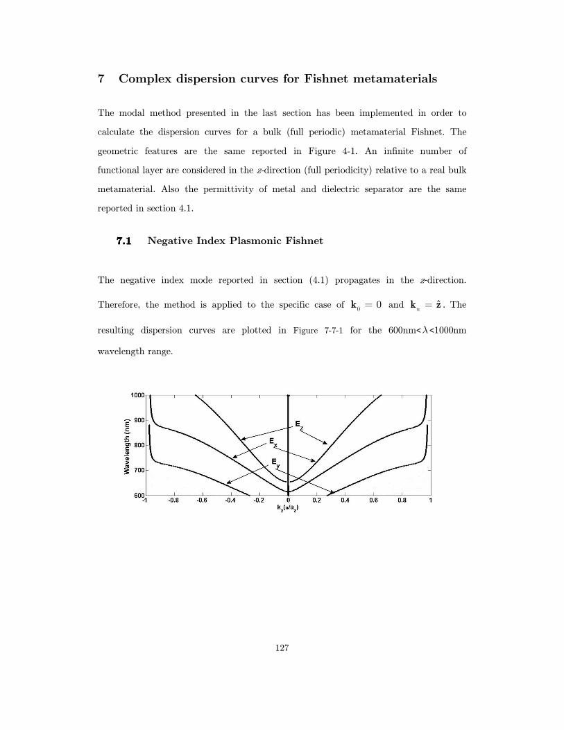
127

7 Complex dispersion curves for Fishnet metamaterials

The modal method presented in the last section has been implemented in order to

calculate the dispersion curves for a bulk (full periodic) metamaterial Fishnet. The

geometric features are the same reported in Figure 4-1. An infinite number of

functional layer are considered in the z-direction (full periodicity) relative to a real bulk

metamaterial. Also the permittivity of metal and dielectric separator are the same

reported in section 4.1.

7.17.17.17.1 Negative Index Plasmonic Fishnet

The negative index mode reported in section (4.1) propagates in the z-direction.

Therefore, the method is applied to the specific case of 0

0=k and ˆk zn= . The

resulting dispersion curves are plotted in Figure 7-7-1 for the 600nm<λ <1000nm

wavelength range.

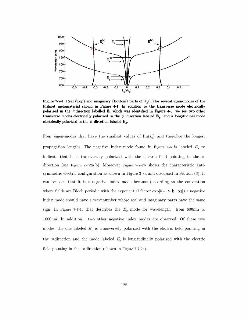
128

Figure Figure Figure Figure 7777----7777----1111: Real (Top) and imaginary (B: Real (Top) and imaginary (B: Real (Top) and imaginary (B: Real (Top) and imaginary (Bottom) parts of ottom) parts of ottom) parts of ottom) parts of ( )zk ω for several eigenfor several eigenfor several eigenfor several eigen----modes of the modes of the modes of the modes of the

FishnetFishnetFishnetFishnet metamaterialmetamaterialmetamaterialmetamaterial shown in shown in shown in shown in Figure Figure Figure Figure 4444----1111. In addition to the transverse mode electrically . In addition to the transverse mode electrically . In addition to the transverse mode electrically . In addition to the transverse mode electrically

polarized in the polarized in the polarized in the polarized in the x direction labelled Edirection labelled Edirection labelled Edirection labelled Exxxx which was identified in which was identified in which was identified in which was identified in Figure Figure Figure Figure 4444----5555, , , , we see two other we see two other we see two other we see two other

transverse modestransverse modestransverse modestransverse modes electrically polarized in the electrically polarized in the electrically polarized in the electrically polarized in the y direction labeled Edirection labeled Edirection labeled Edirection labeled Eyyyy and aand aand aand a longitudinal mode longitudinal mode longitudinal mode longitudinal mode

electrically electrically electrically electrically polarized in the polarized in the polarized in the polarized in the z direction labeled Edirection labeled Edirection labeled Edirection labeled Ezzzz....

Four eigen-modes that have the smallest values of Im(kz) and therefore the longest

propagation lengths. The negative index mode found in Figure 4-5 is labeled Ex to

indicate that it is transversely polarized with the electric field pointing in the x-

direction (see Figure 7-7-2a,b). Moreover Figure 7-7-2b shows the characteristic anti-

symmetric electric configuration as shown in Figure 3-8a and discussed in Section (3). It

can be seen that it is a negative index mode because (according to the convention

where fields are Bloch periodic with the exponential factor exp[i(ω t- k k k k · xxxx)]) a negative

index mode should have a wavenumber whose real and imaginary parts have the same

sign. In Figure 7-7-1, that describes the Ex mode for wavelength from 600nm to

1000nm. In addition, two other negative index modes are observed. Of these two

modes, the one labeled Ey is transversely polarized with the electric field pointing in

the y-direction and the mode labeled Ez is longitudinally polarized with the electric

field pointing in the zzzz----direction (shown in Figure 7-7-2c).

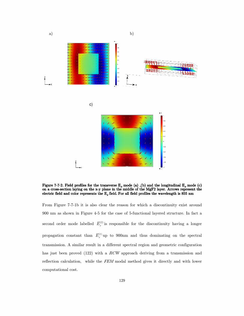
129

a) b)

c)

Figure Figure Figure Figure 7777----7777----2222. . . . Field profiles forField profiles forField profiles forField profiles for the transverse Ethe transverse Ethe transverse Ethe transverse Exxxx mode (amode (amode (amode (a) ) ) ) ,(b) ,(b) ,(b) ,(b) and the longitudinal Eand the longitudinal Eand the longitudinal Eand the longitudinal Ezzzz mode (cmode (cmode (cmode (c) ) ) ) on a crosson a crosson a crosson a cross----section laying on the section laying on the section laying on the section laying on the xxxx----y y y y plaplaplaplane in the middle ne in the middle ne in the middle ne in the middle of the MgF2 layer. Arrows represent of the MgF2 layer. Arrows represent of the MgF2 layer. Arrows represent of the MgF2 layer. Arrows represent the the the the electric field and color represents the Eelectric field and color represents the Eelectric field and color represents the Eelectric field and color represents the Ezzzz field.field.field.field. For all fielFor all fielFor all fielFor all field profiles the wavelength is d profiles the wavelength is d profiles the wavelength is d profiles the wavelength is 855855855855 nmnmnmnm From Figure 7-7-1b it is also clear the reason for which a discontinuity exist around

900 nm as shown in Figure 4-5 for the case of 5-functional layered structure. In fact a

second order mode labelled (2)x

E is responsible for the discontinuity having a longer

propagation constant than (1)x

E up to 900nm and thus dominating on the spectral

transmission. A similar result in a different spectral region and geometric configuration

has just been proved (122) with a RCW approach deriving from a transmission and

reflection calculation, while the FEM modal method gives it directly and with lower

computational cost.

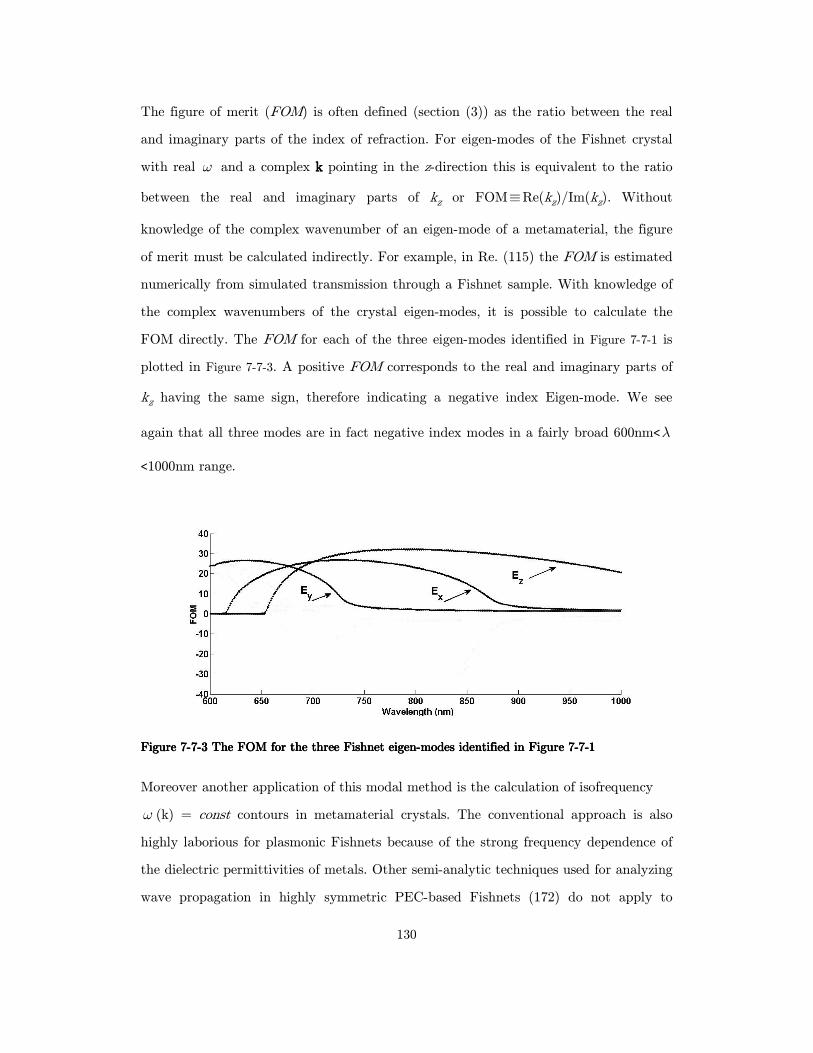
130

The figure of merit (FOM) is often defined (section (3)) as the ratio between the real

and imaginary parts of the index of refraction. For eigen-modes of the Fishnet crystal

with real ω and a complex k k k k pointing in the z-direction this is equivalent to the ratio

between the real and imaginary parts of kz or FOM≡Re(kz)/Im(kz). Without

knowledge of the complex wavenumber of an eigen-mode of a metamaterial, the figure

of merit must be calculated indirectly. For example, in Re. (115) the FOM is estimated

numerically from simulated transmission through a Fishnet sample. With knowledge of

the complex wavenumbers of the crystal eigen-modes, it is possible to calculate the

FOM directly. The FOM for each of the three eigen-modes identified in Figure 7-7-1 is

plotted in Figure 7-7-3. A positive FOM corresponds to the real and imaginary parts of

kz having the same sign, therefore indicating a negative index Eigen-mode. We see

again that all three modes are in fact negative index modes in a fairly broad 600nm<λ

<1000nm range.

Figure Figure Figure Figure 7777----7777----3333 The FOM for the three The FOM for the three The FOM for the three The FOM for the three FishnetFishnetFishnetFishnet eigeneigeneigeneigen----modes identifiedmodes identifiedmodes identifiedmodes identified in in in in Figure Figure Figure Figure 7777----7777----1111

Moreover another application of this modal method is the calculation of isofrequency

ω (k) = const contours in metamaterial crystals. The conventional approach is also

highly laborious for plasmonic Fishnets because of the strong frequency dependence of

the dielectric permittivities of metals. Other semi-analytic techniques used for analyzing

wave propagation in highly symmetric PEC-based Fishnets (172) do not apply to

131

plasmonic Fishnets of interest. Moreover the FEM method provides information

about propagation lengths which are important in lossy metamaterials such as the

Fishnet. Figure 7-7-4 shows an iso-frequency diagram calculated using the FEM modal

method. A single isofrequency contour was obtain by fixing the real frequency ω ,

setting 0 yk= ˆk y and n= ˆk z , and then scanning ky from π− /py to π /py.

a) b)

Figure Figure Figure Figure 7777----7777----4444.... (a)(a)(a)(a)IsoIsoIsoIso----frequency contours for the Efrequency contours for the Efrequency contours for the Efrequency contours for the Ex x x x polarized eigenpolarized eigenpolarized eigenpolarized eigen----mode of the mode of the mode of the mode of the FishnetFishnetFishnetFishnet crystal crystal crystal crystal plotted with respect to Replotted with respect to Replotted with respect to Replotted with respect to Re((((kkkkzzzz) ) ) ) and and and and kkkkyyyy. The black arrows indicate the direction of the. The black arrows indicate the direction of the. The black arrows indicate the direction of the. The black arrows indicate the direction of the phase phase phase phase velocity and the red arrows indicate the direction of thvelocity and the red arrows indicate the direction of thvelocity and the red arrows indicate the direction of thvelocity and the red arrows indicate the direction of the group velocity at a wavelength of e group velocity at a wavelength of e group velocity at a wavelength of e group velocity at a wavelength of

820820820820nmnmnmnm and and and and kkkkyyyy ====wwww////ccccsinsinsinsin((((π ////6666))))....(b) Iso(b) Iso(b) Iso(b) Iso----frequency contours for the imaginary part frequency contours for the imaginary part frequency contours for the imaginary part frequency contours for the imaginary part of kof kof kof kyyyy. The . The . The . The EEEExxxx

eigeneigeneigeneigen----modesmodesmodesmodes are represented with colors: (magenta) 620nm, (black) 630 nm, (cyan) 640 nm, are represented with colors: (magenta) 620nm, (black) 630 nm, (cyan) 640 nm, are represented with colors: (magenta) 620nm, (black) 630 nm, (cyan) 640 nm, are represented with colors: (magenta) 620nm, (black) 630 nm, (cyan) 640 nm, (blue) 650nm.(blue) 650nm.(blue) 650nm.(blue) 650nm.

The eigenvalue in this simulation is a complex valued kz. This procedure was repeated

for several values of wavelength from 620nm to 650nm. The resulting eigen-modes can

be excited by a plane wave incident on an interface between vacuum and the Fishnet

crystal parallel with the x-y plane if the wave-vector of the incident wave is confined to

the y-z plane. Because the y-component of the incident wave-vector is real valued, the

y-component of the wave excited in the Fishnet crystal must also be real-valued.

ky = sin θ (ω /c) where θ is the incidence angle with respect to the normal z. The

eigenmode excited in the Fishnet crystal decays in the z-direction as indicated by the

imaginary part of kz plotted in Figure 7-7-4b. The iso-frequency contours in Figure

7-7-4 are hyperbolic in appearance. For ky =(ω /c)sin(π /6) and a wavelength of

630nm the iso-frequency diagram shows two eigen-modes with the correct value of ky

and equal and opposite values of kz. The correct mode is found by calculating the

group velocity Re( )gv ω≡ ∂ ∂/ k which is by definition normal to the iso-frequency

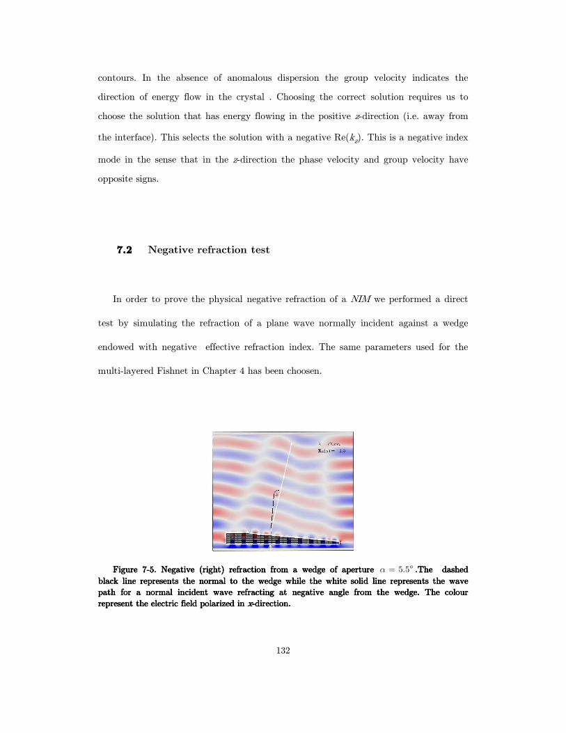
132

contours. In the absence of anomalous dispersion the group velocity indicates the

direction of energy flow in the crystal . Choosing the correct solution requires us to

choose the solution that has energy flowing in the positive z-direction (i.e. away from

the interface). This selects the solution with a negative Re(kz). This is a negative index

mode in the sense that in the z-direction the phase velocity and group velocity have

opposite signs.

7.27.27.27.2 Negative refraction test

In order to prove the physical negative refraction of a NIM we performed a direct

test by simulating the refraction of a plane wave normally incident against a wedge

endowed with negative effective refraction index. The same parameters used for the

multi-layered Fishnet in Chapter 4 has been choosen.

Figure Figure Figure Figure 7777----5555. . . . NNNNegative (right) refractionegative (right) refractionegative (right) refractionegative (right) refraction from a wedge of aperture from a wedge of aperture from a wedge of aperture from a wedge of aperture 5.5α = ° .The dashed .The dashed .The dashed .The dashed

black line represents the normal to the wedge while the white solid line represents the wave black line represents the normal to the wedge while the white solid line represents the wave black line represents the normal to the wedge while the white solid line represents the wave black line represents the normal to the wedge while the white solid line represents the wave

path for path for path for path for a a a a normal incident wave refracting at negative angle from the wedge.normal incident wave refracting at negative angle from the wedge.normal incident wave refracting at negative angle from the wedge.normal incident wave refracting at negative angle from the wedge. The colour The colour The colour The colour

represent the electric field polarizerepresent the electric field polarizerepresent the electric field polarizerepresent the electric field polarized in d in d in d in xxxx----direction.direction.direction.direction.

133

The wedge consist of 21 layers (at its maximum height) scaled down to 5 layers (at

its minimum height). The wedge aperture is 5.5α = ° . The effective refraction index

for a N=10 functional layers structure at 720nm was first calculated , where the valued

retrieved for the refractive index is Re(n)= -1.5, see Figure 7-6. Note that the 5-

functional layers structure in Figure 4-5 overwrites well to the 10-functional layers

structure refractive index showed in Figure 7-6 proving that just for few layers (at

least 7 layers) the asymptotic bulk value is well reached. The predicted angle of

refraction is calculated by Snell’s law, sin( ) / sin( )n ϑ α= . For Re(n)=-1.5 it is

8ϑ− ≈ ° which describes the simulated out-going wave direction at negative angle.

Moreover from the extraction of the scattered electric field polarization (retrieved with

COMSOL) the field components (x- and z- components respectively) have been

averaged in order to find the average polarization which gives us a value of 9.2°

comparable with the previous calculated of 8°. The little mismatch can be due to the

finiteness of the prism size and to edge diffractions.

Figure Figure Figure Figure 7777----6666. Retrieved effective refractive index for a . Retrieved effective refractive index for a . Retrieved effective refractive index for a . Retrieved effective refractive index for a NNNN=10 functional layer structure. =10 functional layer structure. =10 functional layer structure. =10 functional layer structure.

134

7.37.37.37.3 Conclusion

The application of the FEM modal method to the Fishnet metamaterial clearly show

that the bulk-structure is strongly dispersive. Three negative-index modes of the

Fishnet structure and hyperbolic iso-frequency surfaces have been computed for the

least-damped transverse mode. The method represent a powerful tool because it

directly allows the extraction of the imaginary part of the refractive index and

consequently its FOM and the possibility to distinguish between the dominant modes

inside the metamaterial.

135

8 Conclusion

The aim of this doctoral thesis has been to study the propagation of electromagnetic

waves in periodic structures, namely in Fishnet metamaterial. These new class of

materials possesses uncommon properties in nature and one could say that

metamaterials have formed a new research direction in recent years. It has been

investigated on the origin and the manipulation of the negative refractive index both in

a double-layered structure and a bulk multi-layered system. The refractive index of a

metamaterial fishnet in the long wavelength regime is an effective parameter of the

system. However, the current homogeneous methods for the extraction of the effective

fishnet parameters are not sufficient to understand all the complex properties of the

structure. The main contribute of the thesis is a clear presentation of a powerful modal

method in the Finite Element environment. This method allows the comprehension of

the Fishnet modes from a microscopically point of view. It enables the possibility to

calculate all the complex Bloch modes (real and imaginary part) and the complex

isofrequency contours, being both a crucial point when dissipation is present in

metamaterials. This method amply discussed in (148) has been extended to embrace a

wide class of plamonic and photonic crystal slabs. The introductory part of the thesis

gives a brief historical overview of metamaterial research. The main research directions

in this area are outlined, together with a list of crucial papers published in each subject

field in recent years. In Chapter 2 we reported the general tools for the extraction of

the effective parameters for isotropic and bianistropic metamaterials at normal

incidence and at large wavelength regime ( dλ ≫ ). The choice of multi-branch in the

real part of the effective refractive index requires much attention and some artifacts

can be produced around the resonance wavelength (resonant – anti-resonant behavior

between permittivity and permeability) due to the intrinsic periodicity of the structure.

In Chapter 3 the Fishnet structure is built by crossed metallic wires separated by a

dielectric spacer. The connection of the wires forms a slab pair. The slab behaves as a

136

resonant magnetic-moment element generated by opposed currents between the double

interface metal-dielectric forming a magnetic dipole loop. While negative permittivity is

easily obtained by using the most common metals, achieving negative permeability is

requires more efforts. The presence of wide slabs in the Fishnet structure allows a large

filling factor (F) and thus a strong magnetic response. Moreover the connection with

continuous wires pushes the lower resonant electric mode of the structure much above

the magnetic resonance regime, leading to a perfect overlapping between negative

permeability and negative permittivity at the magnetic resonance. For this reason the

Fishnet structure seems to be a prominent candidate for achieving LH metamaterials.

We have reported a design and a parametrical analysis of a Fishnet in the optical

spectral range. In particular the dependence of both the magnetic and the electric

resonance on the geometric features of the Fishnet is investigated. We found that a

sharp electric resonance is down-shifted by 200 nm related to weakening of the

magnetic resonance. For appropriately designed squared hole-array structures, the

frequency of the magnetic resonance coincides with a region of negative effective

permittivity and a negative index of refraction is seen in the simulations. We use the

LC circuit description proposed for comparing the simulated results with the analytic

predictions and to reduce the time needed to design practical applications using the

proposed line. Hence we have a clear understanding of the parametric space over which

it is possible to optimize the Fishnet NIM and the related applications. In Chapter 4 we

studied how the effective optical parameters change as the number of layers increases.

The number of layers required to reach the bulk 3D regime strongly depends on the

coupling between adjacent layers, and hence on the interlayer spacing. If the distance

between adjacent functional layers is small, the coupling is strong, the convergence of

the optical properties is slow, and at least four functional layers are required. The

behavior converges, but not to that of the monolayer case. In contrast, for larger

distances, the coupling is weak and the retrieved optical parameters for several

functional layers are very similar to that of the monolayer case (173). The retrieved

effective parameters remain the same when increasing the number of layers, which

means that the bulk metamaterial limit has been reached. The minimum number of

137

layers required for the metamaterial to qualify as ‘bulk’ depends on both the structure

under investigation and the choice of az. Moreover we employed a modal analysis in

order to make evidence of the evanescent internal and external SPPs modes of the

multi-layered structure based on the approximation between the multi-layered Fishnet

metamaterial and the multi-layered flat system (equaling the external momentum of

the incident light to the kkkk(ω ) dispersion curve of a multi-layered flat system). We

made evidence of SPPs modes for N= 1-,2-,3-,4- functional layers system noticing that

the 1-layer resonances split into N in the multilayer configuration. In Chapter 5 we

showed how the Focused-ion beam lithography can be used to prepare prototypes of

simple and effective metamaterial structures well known as ‘‘fish-net’’. The prepared

samples were characterized by means of spectroscopic ellipsometry in terms of

transmittance and reflectance measurements. Numerical simulation of the structure

(the transmittance (T) and reflectance (R)) are in good qualitative agreement with

optical measurements in a wide range of wavelengths although a shift in the position of

the peak was observed. A wavelength band of single-negative operation is expected

where the sample exhibits NIM behavior in the infrared at 1200 nm. It has been

showed how bi-anisotropy can sensibly affect the sample. The analytic method

presented in Chapter 2 has been employed for the extraction of the bianisotropic

effective parameters in order to study their behavior for a 1- and 3- functional layered

system. We showed that the magnitude of negative refractive index in NIMs depends

on the sidewall-angle, that is, the minimum value of Re(neff) increases as the SWA

increases as result of the blue-shifted resonance peaks of both Re(µ eff) and Re( ε eff). In

Chapter 6 we have presented a full-vectorial Finite Elements based numerical method

for the modal analysis of 2D and 3D palsmonic/photnonic crystal in presence of

dispersive losses materials. The introduction of PMLs in the weak formulation of the

Helmholtz eigenvalue equation allows the calculation of the complex Bloch dispersion

curves also for plasmonic/photonic crystal slab. The method directly solves a quadratic

eigenvalue problem in kkkk and it naturally allows retrieving both real and imaginary part

138

of Bloch wave vectors, which is of particular interest in analysis of plasmonic

nanostructures.

Moreover the modal method allows the study of leaky modes radiation thus enabling

not only the calculation of the real and imaginary part of the leaky modes but also the

reconstruction of the correct radiative eigen-mode profile. Another powerful application

of the modal method consists in the calculation of the iso-frequency (complex) contour

for any periodic structure, in particular a metamaterial Fishnet (Chapter 7). Several

indirect tests based on the direct illumination and scattering formulation have been

performed confirming the reliability of the method which at our knowledge is one of the

most advanced in terms of computational time, precision and richness of physical

information.

139

9 Bibliography

1. “The electrodynamics of substances with simultaneously negative values of ε and µ”.

V. G. Veselago. 4, s.l. : Soviet Physics Uspekhi, 1968, Vol. 10, pp. 509–514.

2. ”Unusual waveguide characteristics associated with the apparent negative permeability obtainable in ferrites. GHB, Thompson. s.l. : Nature, 1995, Vol. 175, pp.

1135–1136.

3. J. D. Joannopoulos, S. G. Johnson, R. D. Meade, and J. N. Winn. Photonic Crystals:Molding the Flow of Light. Second edition. s.l. : Princeton Univ. Press, 2008.

4. “Metamaterials in electromagnetics (invited review),”. A. Sihvola. 1, s.l. :

Metamaterials, 2007, Vol. 1, pp. 2-11.

5. “On the three different denotations of handedness in wavematerial interaction”. A.

Sihvola and I. Lindell. Pisa : URSI International Symposium on Electromagnetic Theory,

2004, pp. 84-86.

6. Electromagnetic waves in chiral and bi-isotropic media. I. V. Lindell, A. Sihvola, S.

A. Tretyakov, and A. J. Viitanen. Boston & London : Artech House, 1994.

7. “On group-velocity”. Lamb, H. 1, s.l. : Proc. London Math. Soc.,, 1994, pp. 473–479.

8. A. Schuster. ”An Introduction to the Theory of Optics”. London : Edward Arnold,

1904. pp. 607–608.

9. “Growth of a wave-group when the group velocity is negative”. Pocklington, H. C.

s.l. : Nature, 2005, Vol. 71, pp. 607–608.

10. Lectures on some problems of the theory of oscillations. L. I. Mandelshtam.

Moscow : Complete Collection of Works, 1944, Vol. 5.

11. “The energy of electromagnetic waves in dispersive media”. Sivukhin, D. V. s.l. :

Opticheskaia Spektroskopia, 1957, Vol. 3, pp. 308-312.

12. “Magnetism from conductors and enhanced nonlinear phenomena”. J. B. Pendry, A.

J. Holden, D. J. Robbins, and R. J. Stewart. 11, s.l. : IEEE Trans. Microwave Theory

Tech, 1999, Vol. 47, pp. 2075–2084.

13. “Composite medium with simultaneously negative permeability and permittivity”.

D. R. Smith, W. J. Padilla, D. C. Vier, S. C. Nemat-Nasser, and S. Schultz,. 18, s.l. : Phys.

Rev. Lett, May 2000, Vol. 84, pp. 4184–4187.

14. “Negative refraction makes a perfect lens”. Pendry, J. B. 18, s.l. : Phys. Rev. Lett,

October 2000, Vol. 85, pp. 3966–3969.

15. “Negative refractive index in left-handed materials”. Kroll, D. R. Smith and N. 14,

s.l. : Phys. Rev.Lett., Oct. 2000, Vol. 84, pp. 2933–2936.

16. “Direct calculation of permeability and permittivity for a left-handed material”. D.

R. Smith, D. C. Vier, N. Kroll, and S. Schultz. 14, s.l. : Appl. Phys. Lett, Oct. 2000, Vol.

77, pp. 2246–2248.

17. “Experimental verification of a negative index of refraction”. R. A. Shelby, D. R.

Smith, and S. Schultz,. s.l. : Science, April 2001, Vol. 292, pp. 7–79.

140

18. “Analogues of an ionized medium: Applications to the ionosphere”. Bracewell, R. N.

s.l. : Wireless Eng.,, December 1954, Vol. 31, pp. 320-326,.

19. “Plasma simulation by artificial dielectrics and parallel-plate media,”. W. Rotman. 1,

1962 : IRE Trans. Antennas Propag., January, Vols. vol. AP-10, pp. 82-85.

20. “Extremely low frequency plasmons in metallic mesostructures,”. J. B. Pendry, A. J.

Holden, W. J. Stewart, and I. Youngs. 25, s.l. : Phys. Rev. Lett, June 1996, Vol. 76, pp.

4773-4776.

21. “3D wire mesh photonic crystal”. D. F. Sievenpiper, M. E. Sickmiller, and E.

Yablonovitch. 14, s.l. : Phys. Rev. Lett., April 1996, Vol. 76, pp. 2480-2483,.

22. “Magnetism from conductors and enhanced nonlinear phenomena,”. J. B. Pendry, A.

J. Holden, D. J. Robbins, and W. J. Stewart. 11, s.l. : IEEE Trans. Microwave Theory

Tech., November 1999, Vol. 47, pp. 2075-2084,.

23. “Metal lens antennas,”. Kock, W. E. s.l. : Proceedings, IRE and Waves and

Electrons, November 1946, pp. 828-836.

24. “Calculation and measurement of bianisotropy in a split ring resonator

metamaterial,”. D. R. Smith, J. Gollub, J. J. Mock, W. J. Padilla, and D. Schurig. s.l. : J.

Appl. Phys., 2006, Vol. 100, pp. 024 507(1–9).

25. “Electrically small isotropic three dimensional magnetic resonators for metamaterial

design,”. J. D. Baena, L. Jelınek, R. Marques, and J. Zehentner. s.l. : Appl. Phys. Lett.,

2006, Vol. 88, pp. 134 108(1–3).

26. “Refining the perfect lens,”. Ramakrishna, J. B. Pendry and S. A. s.l. : Physica B,

2003, Vol. 338, pp. 329–332.

27. “Limitations on sub-diffraction imaging with a negative refractive index slab,”. D. R.

Smith, D. Schurig, M. Rosenbluth, S. Schultz, S. A. Ramakrishna, and J. B. Pendry. s.l. :

Appl. Phys.Lett., 2003, Vol. 82, pp. 1506–1508.

28. “Spherical perfect lens: Solutions of Maxwells equations for spherical geometry,”.

Pendry, S. A. Ramakrishna and J. B. s.l. : Phys. Rev. B, 2004, Vol. 69, pp. 115 115(1–7).

29. “Overcoming the diffraction limit with a planar lefthanded transmission-line lens,”.

Eleftheriades, A. Grbic and G. V. 11, s.l. : Phys. Rev. Lett., March 2004, Vol. 92, pp. 117

403(1–4).

30. “Near-perfect imaging in a focusing system based on a left-handed-material plate,”.

Kissel, A. N. Lagarkov and V. N. 7, s.l. : Phys. Rev. Lett., Feb. 2004, Vol. 92, pp. 077

401(1–4).

31. “Focusing by planoconcave lens using negative refraction,”. P. Vodo, P. V. Parimi,

W. T. Lu, and S. Sridhar. s.l. : Appl. Phys. Lett., 2005, Vol. 86, pp. 201 108(1–3).

32. “Subwavelength resolution with a negative-index metamaterial siperlens”. K. Aydin,

I. Bulu, and E. Ozbay. s.l. : Appl. Phys. Lett., 2007, Vol. 90, pp. 254 102(1–3).

33. “Negative index lens aberrations,”. Smith, D. Schurig and D. R. s.l. : Phys. Rev. E,

2004, Vol. 70, pp. 065 601(1–4).

34. “Three-dimensional superresolution in metamaterial slab lenses: Experiment and

theory,”. F. Mesa, M. J. Freire, R. Marques, and J. D. Baena. s.l. : Phys. Rev. B, 2005,

Vol. 72.

141

35. “Theory of three-dimensional subdiffraction imaging,”. R. Marques, M. J. Freire,

and J. D. Baena. s.l. : Appl. Phys. Lett., 2006, Vol. 89, pp. 211 113(1–3).

36. “Perturbation on the perfect lens: the near-perfect lens,”. O. E. French, K. I.

Hopcraft, and E. Jakeman. s.l. : New Journal of Phys., 2006, Vol. 8, p. 271.

37. “Terahertz magnetic response from artificial materials,”. T. J. Yen, W. J. Padilla, N.

Fang, D. C. Vier, D. R. Smith, J. B. Pendry, D. N. Basov,and X. Zhang. s.l. : Science,

2004, Vol. 303, pp. 1494–1496.

38. “Magnetic response of metamaterials at 100 terahertz,”. S. Linden, C. Enkrich, M.

Wegener, J. Zhou, T. Koschny, and C. M. Soukoulis. s.l. : Science, 2004, Vol. 306, pp.

1351–1353.

39. “Regenerating evanescent waves from a silver superlsne”. N. Fang, Z. Liu, T.-J. Yen,

and X. Zhang,. 7, s.l. : Optics Express, April 2003, Vol. 11, pp. 682–687.

40. “Subwavelength imaging at infrared frequencies using an array of metallic

nanorods,”. M. G. Silveirinha, P. A. Belov, and C. R. Simovski,. s.l. : Phys. Rev. B, 2007,

Vol. 75, pp. 035 108(1–12).

41. “Subdiffraction-limited optical imaging with a silver superlens,”. N. Fang, H. Lee, C.

Sun, and X. Zhang. s.l. : Science, 2005, Vol. 308, pp. 534–537.

42. “Controlling electromagnetic fields,”. J. B. Pendry, D. Schurig, and D. R. Smith.

s.l. : Science, 2006, Vol. 312, pp. 1780–1782.

43. “Calculation of material properties and ray tracing in transformation media,”. D.

Schurig, J. B. Pendry, and D. R. Smith. [ed.] 9794–9804. 21, s.l. : Optics Express, Oct.

2006, Vol. 14.

44. “Notes on conformal invisibility devices,”. Leonhardt, U. 118, s.l. : New Journal of

Phys.,, 2006, Vol. 8.

45. “Metamaterial electromagnetic cloak at microwave frequencies,”. D. Schurig, J. J.

Mock, B. J. Justice, S. A. Cummer, J. B. Pendry, A. F. Starr, and D. R.Smith. s.l. :

Science, 2006, Vol. 314.

46. “Role of bianisotropy in negative permeability and left-handed metamaterials,”. R.

Marques, F. Medina, and R. Rafii-El-Idrissi. s.l. : Phys. Rev. B, 2005, Vol. 65, pp. 144

440(1–6),.

47. “A chiral route to negative refraction,”. Pendry, J. B. s.l. : Science, November 2004,

Vol. 306, pp. pp. 1353–1355.

48. “Generalized constitutive relations for metamaterials based on the quasi-static

lorentz theory,”. A. Ishimaru, S.-W. Lee, Y. Kuga, and V. Jandhyala. 10, s.l. : IEEE Trans.

Antennas Propagat., October 2003, Vol. 51.

49. “Plane waves with negative phase velocity in isotropic chiral mediums,”. Mackay, T.

G. 2, s.l. : Microwave and Opt. Techn. Lett., April 2005, Vol. 45, pp. 120–121.

50. “Backward-wave regime and negative refraction in chiral composites,”. S. A.

Tretyakov, A. Sihvola, and L. JylhΥa. s.l. : Photonics and Nanostructures, 2005, Vol. 3, pp.

107–115.

51. “Negative refractions in uniaxially anisotropic chiral media,”. Cui, Q. Cheng and T.

J. s.l. : Phys. Rev. B, 2006, Vol. 73, pp. 113 104(1–4).

142

52. “Negative refraction in gyrotropic media,”. V. M. Agranovich, Y. N. Gartstein, and

A. A. Zakhidov. s.l. : Phys. Rev. B, 2006, Vol. 73, pp. 045 114(1–12).

53. “Tunable split-ring resonators for nonlinear negative-index metamaterials,”. I. V.

Shadrivov, S. K. Morrison, and Y. S. Kivshar. 20, s.l. : Optics Express, 2006, Vol. 14, pp.

9344–9349.

54. “Tunable metamaterial transmission lines based on varactor-loaded split-ring

resonators,”. I. Gil, J. Bonache, J. Garcıa-Garcıa, and F. Martın. 6, s.l. : IEEE Trans.

Microwave Theory Tech., 2006, Vol. 55, pp. 2665–2674.

55. A. A. Zharov, I. V. Shadrivov, and Y. S. Kivshar,. s.l. : Phys. Rev. Lett., 2003, Vol.

91.

56. “Electronically controlled phase shifters based on right/left-handed transmission

lines,”. O. G. Vendik, I. B. Vendik, D. V. Kholodnyak, S. P. Zubko, and E. V.

Serebryakova. Paris, France : Proc. of the 35th European Microwave Conference, October

2005, pp. 909–912.

57. “Design and measurement of a smart tunable periodic material,”. L. Mercier, M.

Thevenot, A. Crunteanu, B. Jecko, J. C. Orlienyes, C. Champeaux,A. Caterinot, and P.

Blondy,. Long beach, California : IEEE MTT-S International Microwave Symposium

Digest, 2005.

58. “Liquid-crystal photonic-band-gap materials: The tunable electromagnetic vacuum,”.

John, K. Busch and S. s.l. : Phys. Rev. Lett., 1999, Vol. 83, pp. 967–970.

59. “Tunable refraction effects in two-dimensional photonic crystals utilizing liquid

crystals,”. Yoshino, H. Takeda and K. s.l. : Phys. Rev. E, 2003, Vol. 76, pp. 056 607(1–5).

60. ”Tunable Fishnet metamaterials infiltrated by liquid crystal,”. Alexander Minovich,

Dragomir N. Neshev, David A. Powell, Ilya V. Shadrivov. s.l. : Appl. Physic Tett., 2010,

Vol. 96.

61. “Optical negative-index metamaterials,”. Shalaev, V. M. s.l. : Nature Photonics,

2007, Vol. 1, pp. 41–48.

62. “Terahertz magnetic response from artificial materials,”. T. J. Yen, W. J. Padilla, N.

Fang, D. C. Vier, D. R. Smith, J. B. Pendry, D. N. Basov,and X. Zhang. s.l. : Science,

2004, Vol. 303, pp. 1494–1496.

63. ”Magnetic response of metamaterials at 100 terahertz,”. S. Linden, C. Enkrich, M.

Wegener, J. Zhou, T. Koschny, and C. M. Soukoulis. s.l. : Science, 2004, Vol. 306, pp.

1351–1353.

64. “Midinfrared resonant magnetic nanostructures exhibiting a negative permeability,”.

S. Zhang, W. Fan, N. C. Panoiu, K. J. Malloy, R. M. Osgood, and S. R. J. Brueck. s.l. :

Phys.Rev. Lett., 2005, Vol. 94, pp. 037 402(1–4).

65. “Negative index of refraction in optical metamaterials,”. V. M. Shalaev, W. Cai, U.

K. Chettiar, H.-K. Yuan, A. K. Sarychev, V. P. Drachev, and A. V. Kildishev. s.l. : Optics

Lett., 2005, Vol. 30, pp. 3356–3358.

66. ”Cut-twire pairs and plate pairs as magnetic atoms for optical metamaterials.”. Dolling, G., Enkrich, C., Wegener, M., Zhou, J. F. & Soukoulis, C. M. s.l. : Opt. Lett.,

2005, pp. 3198–3200.

143

67. ”Simultaneous negative phase and group velocity of light in a metamaterial.”. Dolling, G., Enkrich, C., Wegener, M., Soukoulis, C. M. & Linden, S. s.l. : Science, 2006,

Vol. 312, pp. 892–894.

68. ”Negative-index metamaterial at 780 nm wavelength,”. Dolling, G., Wegener, M.,

Soukoulis, C. M. & Linden, S. s.l. : Opt. Lett., 2007, Vol. 32, pp. 53–55.

69. ”Dual-band negative index metamaterial: Double negative at 813 nm and single

negative at 772 nm,”. Chettiar, U. K. et al. s.l. : Opt. Lett., 2007, Vol. 32, pp. 1671–1673.

70. ”A. Double-negative polarization-independent Fishnet metamaterial in the visible spectrum,”. Garcia-Meca, C., Ortuno, R., Rodriguez-Fortuno, F. J., Marti, J. & Martinez.

s.l. : Opt. Lett., 2009, Vol. 34, pp. 1603–1605.

71. ”Yellow-light negative-index metamaterials,”. Xiao, S. M., Chettiar, U. K.,

Kildishev, A. V., Drachev, V. P. & Shalaev, V. M. s.l. : Opt. Lett., 2009, Vol. 34, pp. 3478–

3480 .

72. ”Low-loss multilayered metamaterial exhibiting a negative index of visible of refraction at visible wavelengths,”. Garcia-Meca, C. et al. s.l. : Phys. Rev. Lett., 2011, Vol.

067402.

73. ”Past achievements and future challenges in the development of three-dimensional photonic metamaterials,”. Costas M. Soukoulis, and Martin Wegener. s.l. : Nature, July 17,

2011, Vol. 154.

74. ”Resonant and antiresonant frequency dependence of the effective parameters of metamaterials,”. T. Koschny, P. Markos,*D. R. Smith,and C. M. Soukoulis. s.l. : Physical

Review E, 2003, Vol. 68.

75. 1992. D, Bergman D J and Stroud. 147, s.l. : Solid State Phys, Vol. 46.

76. D, Stroud. 3368, s.l. : Phys. Rev., 1975, Vol. 12.

77. O, Hunderi. 3419, s.l. : Phys. Rev. B, 1973, Vol. 7.

78. W, Milton G. The Theory of Composites. s.l. : Cambridge University Press, 2002.

79. ”Determination of effective permittivity and permeability of metamaterials,”. D. R.

Smith and S. Schultz, P. Markos and C. M. Soukoulis. 195104, s.l. : Phys. Rev. B, April 19,

2002, Vol. 65.

80. ”Impact of inherent periodic structure on effective medium,”. ThP. Markoš, E. N.

Economou, D. R. Smith, D. C. Vier,and C. M. Soukoulis. 245105, s.l. : Phys. Rev. B, 2005,

Vol. 71.

81. ”Robust method to retrieve the constitutive effective parameters of metamaterials,”. Xudong Chen, Tomasz M. Grzegorczyk, Bae-Ian Wu, Joe Pacheco, Jr., and Jin Au Kong.

016608, s.l. : Phys. Rev. B, 2004, Vol. 70.

82. ”Electromagnetic parameter retrieval from inhomogeneous metamaterials,”. D. R.

Smith, D. C. Vier,Th. Koschnyand C. M. Soukoulis. 036617, s.l. : Phys. Rev. E, 2005, Vol.

71.

83. Negative Refractive Index in Optics of Metal-Dielectric composites. A. V. Kildishev,

W. Cai, U. K. Chettiar, H.-K. Yuan, A. K. Sarychev*, V. P. Drachev, and V. M. Shalaev.

s.l. : J. Opt. Soc. Am. B, 2006, Vol. 23, pp. 423-433.

84. ”Bianisotropic Photonic Metamaterials,”. Christine Eliane Kriegler, Michael Stefan

Rill, Stefan Linden, and Martin Wegener. 2, s.l. : IEEE JOURNAL OF SELECTED

TOPICS IN QUANTUM ELECTRONICS,, April 2010, Vol. 16.

85. ”Determination of the effective constitutive parameters of bianisotropic metamaterials,”. Zhaofeng Li, Koray Aydin, and Ekmel Ozbay. 026610, s.l. : Phys. Rev. E,

2009, Vol. 79.

144

86. @, COMSOL Multiphysics. www.comsol.com. [Online] 4.2.

87. Jin, J. The Finite Element Method in Electromagnetics. second edition. s.l. : John

Wiley & Sons, Inc., New York, 2002.

88. Zimmerman, W. B. J. Process Modelling and Simulation with Finite Element Methods. s.l. : World Scientific, Singapore, 2004.

89. Ferrari, P. P. Silvester and R. L. ”Finite elements for electrical engineers,”. 3rd

edition. s.l. : Cambridge University Press, Cambridge, 1996.

90. Kong, J. A. Electromagnetic Wave Theory. s.l. : EMW, Cambridge,MA, 2008.

91. ”A negative permeability material at red light,”. Hsiao-Kuan Yuan, Uday K.

Chettiar, Wenshan Cai, Alexander V. Kildishev,Alexandra Boltasseva*, Vladimir P.

Drachev, and Vladimir M. Shalaev. 3, s.l. : Optics Express, 2007, Vol. 15, pp. 1076-1083.

92. Wenshan Cai, Uday K. Chettiar, Hsiao-Kuan Yuan, Vashista C. de Silva,Alexander

V. Kildishev, Vladimir P. Drachev, and Vladimir M. Shalaev. 6, s.l. : OPTICS EXPRESS,

2007, Vol. 15.

93. Effective Medium Theory of Left-Handed Materials. Kafesaki, T. Koschny and M.

10, s.l. : Phys. Rev. Lett., 2004, Vol. 93, pp. 107402(1-4).

94. ”Design-related losses of double-Fishnet,”. G. Dolling, M.Wegener, C. M. Soukoulis,

and S. Linden. 18, s.l. : Optic express, 2008, Vol. 15, p. 155102.

95. A PERIODIC POROUSNANOSTRUCTURED LEFT-HANDED MATERIAL SLAB AT OPTICALFREQENCIES. Wu, P.-Y. Chen and S.-C. 1, s.l. : microwave and

optical technology letters, 2008, Vol. 50.

96. Optical Constants of Noble Metals. Christy, P.B. Johnson and R.W. 12, s.l. : Phys.

Rev. B, 1972, Vol. 6.

97. Metallic photonic crystals at optical wavelengths. I. El-Kady, M. M. Sigalas, R.

Biswas, K. M. Ho, and C. M. Soukoulis. 23, s.l. : Phys. Rev. B, 2000, Vol. 62, pp. 299-302.

98. A. Christ, T. Zentgraf, S. G. Tikhodeev, N. A. Gippius, O. J. F. Martin, J. Kuhl,

and H. Giessen. s.l. : Phys. Status Solidi B, 2006, Vol. 243, p. 2344.

99. Localized surface-plasmon resonances and negative refractive index in nanostructured electromagnetic metamaterials. J. Parsons, E. Hendry, J. R. Sambles, and

W. L. Barnes. s.l. : Phys. Rev. B, Vol. 80, pp. 245117-.

100. ”Left-handed metamaterials: The Fishnet structure and its variation.”. M.

Kafesaki, I. Tsiapa, N. Katsarakis,Th. Koschny,C. M. Soukoulis,and E. N. Economou. 23,

s.l. : Phys. Rev. B, 2007, Vol. 75, pp. 235114-(1-9).

101. M. Soukoulis, M. Kafesaki, and E. N. Economou,. 1941, s.l. : Adv. Mater., 2006,

Vol. 18.

102. ”Parametric investigation and analysis of Fishnet metamaterials in the microwave regime,”. N.-H. Shen, G. Kenanakis, M. Kafesaki, N. Katsarakis, E. N. Economou,and C.

M. Soukoulis. 12, s.l. : Opt. Soc. of Am. B, 2009, Vol. 26, pp. 61-67.

103. ”Magnetic response of nanoscale left-handed metamaterials,”. R. S. Penciu, M.

Kafesaki, Th. Koschny, E. N. Economou,and C. M. Soukoulis. 23, s.l. : Phys. Rev. B, 2010,

Vol. 81, pp. 235111-(1-11) .

104. Unifying approach to left-handed material design. Jiangfeng Zhou, Eleftherios N.

Economon,Thomas Koschny and Costas M. Soukoulis. 24, s.l. : Opt. Lett., 2006, Vol. 31,

pp. 3620-3622.

105. ”Numerical simulations of terahertz double-negative metamaterial with isotropic-like Fishnet structure,”. P. Ding, E.J. Liang, W.Q. Hu, L. Zhang, Q. Zhou Q.Z. Xue. 2,

s.l. : Photonics and Nanostructures- Fundamental and application, 2009, Vol. 7, pp. 92-100.

145

106. ”Saturation of the Magnetic Response of Split-Ring Resonators at Optical Frequencies,”. 22, s.l. : Phys. Rev. Lett., 2005, Vol. 95, pp. 223902-(1-4).

107. Bruce W. Wessels. s.l. : Annu. Rev. Mater, 2007, Vol. 37, pp. 659-679.

108. M. Maaza, O. Nemraoui, C. Sella,A.C. Beye and B. Baruch-Barak. 1, s.l. : Optics

Communications, 2005, Vol. 254, pp. 188-195.

109. ”Magnetic activity at infrared frequencies in structured metallic photonic crystals,”. R. A. Shelby, D. R. Smith, and S. Schultz. s.l. : J. Phys. Condens. Matter, 2002,

Vol. 14, pp. 6383-6394.

110. ”Numerical investigation of negative refractive index metamaterials at infrared and optical frequencies,”. Osgood, N.-C. Panoiu and R. M. s.l. : Opt. Commun., 2003, pp. 331-

337.

111. ”Magnetic response of split-ring resonators in the far infrared frequency regime,”. N. Katsarakis, G. Konstantinidis, A. Kostopoulos, R. S. Penciu, T. F. Gundogdu, Th

Koschny, M. Kafesaki,E. N. Economou and C. M. Soukoulis. s.l. : Opt. Lett., 2005, Vol. 30,

pp. 1348-1350.

112. ”Demonstration of Near-Infrared Negative-Index Metamaterials,”. S. Zhang, W.

Fan, N. C. Panoiu, K. J. Malloy. s.l. : Phys. Rev. Lett., 2005, Vol. 95.

113. ”Effective parameters of resonant negative refractive index metamaterials: Interpretation and validity,”. D. Seetharamdoo, R. Sauleau, K. Mahdjoubi and A. Tarot.

s.l. : J. Appl. Phys., 2005, Vol. 98, p. 063505.

114. ”Three-dimensional photonic metamaterials at optical frequencies,”. NA LIU,

HONGCANG GUO, LIWEI FU, STEFAN KAISER, HEINZ SCHWEIZER AND

HARALD GIESSEN. s.l. : Nature, 2008, Vol. 7.

115. ”Three-dimensional optical metamaterial with a negative refractive index,”. Jason

Valentine, Shuang Zhang, Thomas Zentgra, Erick Ulin-Avila, Dentcho A. Genov, Guy

Bartal and Xiang Zhang. s.l. : Nature, 2008, Vol. 455.

116. ”Transition from thin-film to bulk properties of metamaterials,”. Carsten

Rockstuhl, † Thomas Paul, and Falk Lederer, Thomas Pertsch,Thomas Zentgraf,* Todd P.

Meyrath, and Harald Giessen. 3, s.l. : Phys. Rev. B, 2008, Vol. 77, pp. 035126-(1-9).

117. ”Plasmonic Building Blocks for Magnetic Molecules in Three-Dimensional Optical Metamaterials,”. Na Liu, Liwei Fu, Stefan Kaiser, Heinz Schweizer, and Harald Giessen. 20,

s.l. : Adv. Mater., Vol. 2008, pp. 3859–3865.

118. H. Liu, D. A. Genov, D. M. Wu, Y. M. Liu, Z. W. Liu, C. Sun, S. N.Zhu, X.

Zhang. 76, s.l. : Phys. Rev., 2007, Vol. B, p. 073101.

119. N. Liu, H. C. Guo, L. W. Fu, S. Kaiser, H. Schweizer, H. Giessen, Nat. s.l. :

Nat.Mater., 2007, Vol. 19, p. 3628.

120. P. Atkins, J. D. Paula. Physical Chemistry. 8th edition. Oxford : Oxford

University Press, 2006.

121. P. Nordlander, C. Oubre, E. Prodan, K. Li, M. I. Stockman. s.l. : Nano Lett., 2004,

Vol. 4, p. 899.

122. ”Optical negative-index bulk metamaterials consisting of 2D perforated metal-dielectric stacks,”. Shuang Zhang, Wenjun Fan, N. C. Panoiu,K. J. Malloy,R. M.

Osgood,and S. R. J. Brueck. 15, s.l. : Opt. Expr., Vol. 14, p. 6779.

123. Ritchie, 1R. H. 874, s.l. : Phys. Rev., 1957, Vol. 106.

124. T. W. Ebbesen, H. J. Lezec, H. F. Ghaemi, T. Thio, and P. A.Wolf. 667, s.l. :

Nature, 1998, Vol. 391.

125. Light passing through subwavelength apertures. F. J. Garcia-Vidal, L. Martin-

Moreno,T. W. Ebbesen,L. Kuipers. s.l. : Rev. Of Mod. Phys., 2010, Vol. 82.

146

126. Raether, H. Surface Plasmons on Smooth and Rough Surfaces and on gratings. s.l. : Springer Tracts in Modern Physics, 1988. Vol. 111.

127. ”Surface Plasmon in thin films,”. Economu, E.N. 2, s.l. : Phys. Rev. , 1969, Vol.

182.

128. ”Role of surface plasmon polaritons on optical transmission through double layer

metallic hole arrays,”. R. Ortuño, C. García-Meca, F. J. Rodríguez-Fortuño, J. Martí, and

Alejandro Martínez. 7, s.l. : Phys. Rev. B, Vol. 79, pp. 075425-(1-10).

129. L. Martín-Moreno, F. J. García-Vidal, H. J. Lezec, K. M. Pellerin,T. Thio, J. B.

Pendry, and T. W. Ebbesen. s.l. : Phys. Rev. Lett., 2011, Vol. 86, p. 1114.

130. ”Double-negative polarization-independent Fishnet metamaterial in the visible

spectrum,”. C. García-Meca, * R. Ortuño, F. J. Rodríguez-Fortuño, J. Martí, and A.

Martínez. 10, s.l. : Opt. Lett., 2009, Vol. 34.

131. 14. C. Enkrich, 1M. Wegener,S. Linden,2S. Burger,L. Zschiedrich,F. Schmidt,J. F.

Zhou,Th.Koschny, and C. M. Soukoulis,. s.l. : Phys. Rev. Lett., 2005, Vol. 95, p. 203901.

132. Uday K. Chettiar, Alexander V. Kildishev, Hsiao-Kuan Yuan, Wenshan Cai,

Shumin Xiao,Vladimir P. Drachev, and Vladimir M. Shalaev. 12, s.l. : Optic letters, 2007,

Vol. 32.

133. . S. Zhang, W. Fan, N. C. Panoiu, K. J. Malloy, R. M. Osgood, and S. R. J.

Brueck. s.l. : Phys. Rev. Lett., 2005, Vol. 95, p. 137404 .

134. “Comparison of negative refractive index materials with circular, elliptical and

rectangular holes,”. Brueck, Z. Ku and S. R. J. s.l. : Opt. Express, 2007, Vol. 15, pp. 4515-

4522.

135. “Realization of three-functional-layer negative-index photonic metamaterial,”. G.

Doling, M. Wegener and S. Linden. s.l. : Opt. Lett., 2007, Vol. 32, pp. 551-553.

136. ”Optical metamaterials at near and mid-IR range fabricated by nanoimprint lithography,”. W. Wu, E. Kim, E. Ponizovskaya, Y. Liu, Z. Yu , N. Fang, Y. R. Shen, A.

M. Bratkovsky, W. Tong, C. Sun,X. Zhang , S. Y. Wang and R. S. Williams. s.l. : Appl.

Phys.A, 2007, Vol. 87, pp. 143-150.

137. ”An efficient way to reduce losses of left-handed metamaterials,”. J. Zhou, T.

Koschny and C. M. Soukoulis. s.l. : Opt. Express., 2008, Vol. 16, pp. 11147-11152.

138. ”Bi-anisotropy of multiple-layer Fishnet negative index metamaterials due to angled sidewalls,”. Zahyun Ku, Jingyu Zhang, and S. R. J. Brueck. 8, s.l. : Opt. Express.,

2009, Vol. 17.

139. “Plasmonics for improved photovoltaics,”. Polman, 3. H. A. Atwater and A. s.l. :

Nat. Mater., 2010, Vol. 9, pp. 205-213.

140. “Nano-optics of surface plasmon polaritons,”. 4. A. V. Zayats, I. I. Smolyanov, A.

A. Maradudin. s.l. : Phys. Rep., 2005, Vol. 408.

141. Sakoda, 11. K. Optical Properties of Photonic Crystal. s.l. : (New York: Springer,

2001), 2001.

142. “Algorithms for the nonlinear eigenvalue problem,”. Ruhe, 12. A. s.l. : SIAM J.

Numer. Anal. , 1973, Vol. 10, pp. 674-689.

143. “Tunneling in photonic band structures,” . Yu, 13. T. Suzuki and P. L. s.l. : J. Opt.

Soc. Am. B, 1995, Vol. 12, p. 804.

144. “Behavior of light at photonic crystal interfaces,”. E. Istrate, A. A. Green, and E.

H. Sargent. s.l. : Phys. Rev. B, 2005, Vol. 71, p. 195122.

147

145. “Revised plane wave expansion method for dispersive material and its application

to band structure calculation of photonic crystal slabs,”. S. Shi, C. Chen and D. Prather.

s.l. : Appl. Phys. Lett., 2005, Vol. 86, p. 043104.

146. “Aplication of finite element methods to photonic crystal modelling,”. B. P. Hiett,

B. D. H., S. J. Cox, J. M. Generowicz, M. Molinari, and K. S. Thomas. s.l. : IEE Proc - Sci.

Meas. Technol, 2002, Vol. 149, pp. 293-296.

147. “The complex bloch bands of a 2D plasmonic crystal displaying isotropic negative

refraction,”. M. Davanco, Y. Urzhumov, and G. Shvets. s.l. : Opt. Express, 2007, Vol. 15,

pp. 9681–9691.

148. “Complex k band diagrams of 3D metamaterials/photonic crystals,”. C. Fietz, Y.

Urzhumov, and G. Shvets. 20, s.l. : Opt. Express,, 2011, Vol. 19, pp. 19027-19041.

149. Stakgold, I. Boundary Value Problem of Mathematical Physics,”. s.l. : New York:

Macmillan, 1968. Vol. 2.

150. ”The quadratic eigenvalue problem,”. Meerbergen, F. Tisseur and K. s.l. : SIAM

Review, 2001, Vol. 43, pp. 235–286.

151. ”Biosensing with plasmonic nanosensors,”. J. N. Anker, W. P. Hall, O. Lyandres,

N. C. Shah, J Zhao and R. P. Van Duyne. s.l. : Nat. Mater., 2008, Vol. 7, pp. 442-453.

152. “Plasmonics for improved photovoltaics,”. Polman, H. A. Atwater and A. s.l. : Nat.

Mater., 2010, Vol. 9, pp. 205-213.

153. M. L. Brongersma, P. G. Kik. Surface Plasmon Nanophotonics. s.l. : Springer,

2007.

154. ”Holey metal films: From extraordinary transmission to negative-index behavior,”. A. Mary, Sergio G. Rodrigo, L. Martin-Moreno, and F. J. Garcia-Vidal. [ed.] 80. s.l. : Phys.

Rev. B, 2009, p. 165431.

155. K. Sakoda. Optical Properties of Photonic Crystals. Berlin : Springer-Verlag, 2001.

156. ”Electric and magnetic properties of sub-wavelength plasmonic crystals,”.

Urxhumov, Gennady Shvets and Yaroslav A. s.l. : J.Opt. A: Pure Appl. Opt., 2005, Vol. 7,

pp. S23-S311.

157. ”A perfectly matched anisotropic absorber for use as an abosrbing boundary condition,”. Sacks, Z. S., Kingsland, D. M., Lee, R. and Lee, Jin-Fa. 12, s.l. : IEEE

Transactions on Antennas and Propagation, 1995, Vol. 43, pp. 1460-1463.

158. ”An Anisotropic Perfectly Matched Layer-Absorbing Medium for the Truncation of FDTD Lattices,”. Stephen D., Gedney. 12, s.l. : Transactions on Antennas and

Propagation, 1996, Vol. 44, pp. 1630-1639.

159. Palik, Edward D. ”Handbook of optical constants of solids,”. s.l. : Academic Press.

160. Accurate determination of quality factor of axisymmetric resonators byperfectly mathed layer. Kirk, M.Imran and Andrew G. s.l. : arXiv:1101.1984v2, 2011.

161. ”Physical origin of photonic energy gaps in the propagation of surface plasmons on gratings,”. W.L.Barnes, T.W. Preist, S.C. Kitson, and J.R. Sambles. 9, s.l. : Physical

Review B, 1996, Vol. 54.

162. ”Corrugated dielectric Waveguides: A numerical Study of the Second-Order Stop

bands,”. M.Neviere, P.Vincent and. s.l. : Appl. Phys., 1979, Vol. 20, pp. 345-351.

163. ”Optical properties of deep lamellar grating: a coupled Bloch-mode insight,”. P.

Lalanne, J.P.Hugonin and P. Chavel. 6, s.l. : Journal of Lightwave technology, 2006, Vol.

24, pp. 2442-2449.

148

164. ”Band gaps and leaky-wave effect in resonant photonic-crystal waveguide,”.

Magnusson, Y.Ding and R. 2, s.l. : Opt. Express, Vol. 15, pp. 608-694.

165. ”Beaming of light at broadside through a subwavelength hole: Leaky wave model and open stopband effect,”. D.R. Jackson, A.A. Oliner T. Zhao and J.T. Williams. 40, s.l. :

RADIO SCIENCE, 2005, Vol. 12.

166. ”The role of leaky plasmon waves in the directive beaming of light through a subwavelength aperture,”. D. R. Jackson, 1J. Chen, R. Qiang, F. Capolino, and A. A.

Oliner. 26, s.l. : Optics Express, 2008, Vol. 16, pp. 21271-21281.

167. ”Extraordinary Transmission of metal films with array of subwavelength holes,”. James V. Coe, Joseph M. Heer, Shannon Teeters-KKennedy, Hong Tian and Kenneth R.

Rodriguez. s.l. : Annu. Rev. Phys. Chem, 2008, Vol. 59, pp. 179-202.

168. ”Mimicking Surface Plasmons with Structured Surfaces,”. J. B. Pendry1, L.

Martín-Moreno and F. J. Garcia-Vidal. 5685, s.l. : Science, 2004, Vol. 305, pp. 847-848.

169. ”Theory of extraordinary optical transmission through subwavelength hole arrays,”. L. Martin-Moreno, F.J. Garcia, H.J. Lezec and T.W. Ebbesen. s.l. : Physical

review letters, 2001, Vol. 6, pp. 114-117.

170. ”Microscopic theory of the extraordinary optical transmission,”. Haitao Liu,

Philippe Lalanne. s.l. : Nature, 2008, Vol. 452, pp. 728-731.

171. Stefan A. Maier, ”Plasmonics. Foundamentals and applications. s.l. : Springer New

York.

172. “Fishnet metamaterials - rules for refraction and limits of homogenization,”. L.

Jelinek, R. Marques, and J. Machac. s.l. : Opt. Express, 2010, Vol. 18, pp. 17940–17949.

173. ”Negative refractive index response of weakly and strongly coupled optical metamaterials,”. Jiangfeng Zhou, Thomas Koschny, Maria Kafesaki, and Costas M.

Soukoulis. s.l. : Phys. Rev. B, 2009, Vol. 80, p. 035109.