PROPAGATION IN NETWORKS WILHELMUS … · WILHELMUS HUBERTUS (WOUTER) VERMEER Propagation in...
234
WILHELMUS HUBERTUS (WOUTER) VERMEER Propagation in Networks The Impact of Information Processing at the Actor Level on System-wide Propagation Dynamics
Transcript of PROPAGATION IN NETWORKS WILHELMUS … · WILHELMUS HUBERTUS (WOUTER) VERMEER Propagation in...
WILHELMUS HUBERTUS (WOUTER) VERMEER
Propagation in NetworksThe Impact of Information Processing at theActor Level on System-wide Propagation Dynamics
WILH
ELM
US H
UB
ERTU
S (W
OU
TER
) VERM
EER
- Pro
pag
atio
n in
Netw
ork
s
ERIM PhD SeriesResearch in Management
Era
smu
s R
ese
arc
h In
stit
ute
of
Man
ag
em
en
t-
373
ERIM
De
sig
n &
la
you
t: B
&T
On
twe
rp e
n a
dvi
es
(w
ww
.b-e
n-t
.nl)
Pri
nt:
Ha
vek
a
(w
ww
.ha
vek
a.n
l)PROPAGATION IN NETWORKSTHE IMPACT OF INFORMATION PROCESSING AT THE ACTOR LEVEL ON SYSTEM-WIDE PROPAGATION DYNAMICS
This thesis addresses the analysis of system-wide dynamics of propagation in networks.It argues that an emphasis should be placed on the mechanism by which propagation takesplace between actors on the micro level. This mechanism is critical in order to understandsystem-wide propagation dynamics. This thesis puts forward the information processingview of propagation, a framework in which describes this mechanism using three distinctsub-processes of propagation; Radiation, Transmission and Reception. Decomposing thepro pa ga tion mechanism into three sub-processes yields a more detailed and methodologi -cally stronger model of propagation which is better suited for capturing the complexity ofthe propagation processes in practice; the RTR-model of propagation. Agent-based simula -tions adopting this model show that distinguishing the three sub-process of propagationis critical in order to: 1) understand the effects of interventions in the propagation process,2) incorporate the heterogeneous behavior of actors, and 3) understand the role of thenetwork structure in propagation.
The Erasmus Research Institute of Management (ERIM) is the Research School (Onder -zoek school) in the field of management of the Erasmus University Rotterdam. The foundingparticipants of ERIM are the Rotterdam School of Management, Erasmus University (RSM),and the Erasmus School of Econo mics (ESE). ERIM was founded in 1999 and is officiallyaccre dited by the Royal Netherlands Academy of Arts and Sciences (KNAW). The researchunder taken by ERIM is focused on the management of the firm in its environment,its intra- and interfirm relations, and its busi ness processes in their interdependentconnections.
The objective of ERIM is to carry out first rate research in manage ment, and to offer anad vanced doctoral pro gramme in Research in Management. Within ERIM, over threehundred senior researchers and PhD candidates are active in the different research pro -grammes. From a variety of acade mic backgrounds and expertises, the ERIM commu nity isunited in striving for excellence and working at the fore front of creating new businessknowledge.
Erasmus Research Institute of Management - Rotterdam School of Management (RSM)Erasmus School of Economics (ESE)Erasmus University Rotterdam (EUR)P.O. Box 1738, 3000 DR Rotterdam, The Netherlands
Tel. +31 10 408 11 82Fax +31 10 408 96 40E-mail [email protected] www.erim.eur.nl
Erim - 15 omslag Vermeer (15221).qxp_Erim - 15 omslag Vermeer 23-10-15 10:32 Pagina 1
1_Erim_Vermeer Stand.job
Propagation in Networks
The impact of information processing at the actor level on
system-wide propagation dynamics

1_Erim_Vermeer Stand.job
2_Erim_Vermeer Stand.job
Propagation in Networks:The impact of information processing at the actor level
on system-wide propagation dynamics
Propagatie in netwerken
De invloed van informatie verwerking op het actor niveau
op systeembrede propagatie dynamiek.
Thesis
to obtain the degree of Doctor from the
Erasmus University Rotterdam
by command of the
rector magnificus
Prof.dr. H.A.P. Pols
and in accordance with the decision of the Doctorate Board
The public defense shall be held on
Thursday the 17th of December 2015 at 11:30 hrs
by
Wilhelmus Hubertus Vermeer
born in Rotterdam, the Netherlands.
2_Erim_Vermeer Stand.job
Doctoral Committee
Promotor: Prof.mr.dr. P.H.M. Vervest
Other members: Prof.dr.ir. H.W.G.M. van Heck
Prof.dr. W. Rand
Prof.dr. K. Frenken
Copromotor: Dr.ir. O.R. Koppius
Erasmus Research Institute of Management - ERIM
The joint research institute of the Rotterdam School of Management (RSM)
and the Erasmus School of Economics (ESE) at the Erasmus University Rotterdam
Internet: http://www.erim.eur.nl
ERIM Electronic Series Portal: http://repub.eur.nl/pub
ERIM PhD Series in Research in Management, 373
ERIM reference number: EPS-2015-373-LIS
ISBN 978-90-5892-429-2c©2015, Vermeer, Wouter
Design: B&T Ontwerp en advies www.b-en-t.nl
Cover design: Original image c©Francine Vermeer (www.francinevermeer.nl)
This publication (cover and interior) is printed by haveka.nl on recycled paper, Revive R©.
The ink used is produced from renewable resources and alcohol free fountain solution.
Certifications for the paper and the printing production process: Recycle, EU Flower, FSC, ISO14001.
More info: http://www.haveka.nl/greening
All rights reserved. No part of this publication may be reproduced or transmitted in any form or by any means electronic
or mechanical, including photocopying, recording, or by any information storage and retrieval system, without permission
in writing from the author.

3_Erim_Vermeer Stand.job
Acknowledgments
The Ph.D. trajectory has been an amazing journey and now that I am finishing this chap-
ter of my life I would like to acknowledge those people who made it an inspiring, educative
and fun process for me.
The choice to start obtaining a Ph.D. was definitely not an obvious one for me. Those of
you who knew me already before the Ph.D. trajectory know that studying has not always
been my favorite activity. It was only after I started my master program in business
information management that I saw how inspiring actual hard work and in-depth study
could be. To a large extent the courses taught by Eric van Heck, Otto Koppius and Peter
van Baalen, and the process of writing a master thesis where the things that pushed me
intellectually. This push made me realize that I love to study the motives and rationale
behind behavior, and dig deeper than the surface to that which lies underneath. To focus
not simply on knowledge, but on understanding how things work. It is because of my
interactions with these people that I began aspiring an academic career, and therefore
without these people I would not have ended up where I am today. Therefore I first and
foremost would like to thank these people specifically for seeing something in me which
I did not see in myself, for motivating me to consider doing a Ph.D., and for leading me
onto the path I’m on today.
In completing the journey of the Ph.D. process quite some credit is due to my supervi-
sory team Peter Vervest and Otto Koppius. As someone who is known to be somewhat
stubborn, I am sure it has not always been the easiest process for them. Nevertheless
they allowed me to set my own topic of research and take it into a direction in which I
was most interested. They gave me the freedom to do things my way, even though that
might not always have been the most easy, efficient or effective one. They have always
managed to inspire me and get me focused on the end-goal, provided me the opportunity
to explore, and facilitated me to continuously reevaluate my own thinking. They made
me aware of the value of incorporating different perspectives. Observing and experienc-

3_Erim_Vermeer Stand.job
vi Acknowledgments
ing their thinking processes and mentoring behavior has not only made me grow as an
academic, but also as a person.
A large amount of credit is due to Bill. First, for being both willing and able to supervise
me at a critical stage point in the trajectory, providing me with crucial feedback. Second,
for hosting me at the University of Maryland, which not only allowed me to experience
the US academic culture, but also to learn from his openness, ability to bridge different
fields, and for the possibility to obtain yet another perspective on doing research. I am
incredibly grateful for the pivotal role he has played in getting me my current job.
Apart from my supervisory team I would also like to thank my committee members; Eric
van Heck, Bill Rand, Koen Frenken, Rob Zuidwijk, Piet van Mieghem and Uri Wilensky
for their willingness and enthusiasm to participate in the public defense.
I would also like to thank Mark Boons and Ting Li. Although they were not formally
part of my supervisory team they have always been very approachable and open; ready
to provide me with advice, feedback and guidance whenever I needed it.
I would like to also acknowledge the support obtained by the Erasmus Research Insti-
tute of Management (ERIM) and the Netherlands Organisation for Scientific Research
(NWO). ERIM’s financial support has enabled me to go to conferences, follow courses
(both internal and external), and build my academic network. NWO has allowed me to
be part of the Complexity research group, introducing me to the theme of complexity and
the multidisciplinary nature of the research field — both of which ended up shaping my
research interests.
For bestowing upon me his view on teaching, Otto deserves a special word of thanks. By
easing me into teaching and letting me experience it from the early stage in my Ph.D.
(while providing me with continuous feedback), he allowed me to see and learn how to
best transfer information. Emphasizing both how to send information and how it can
and will be received, has not only inspired part of my research, but also taught me a skill
which has proven valuable in teaching and coaching students of my own, and in reflecting
upon myself.
In considering the success of my Ph.D. trajectory, my peers should definitely be men-
tioned. Not only have they always been there to provide their perspective, they to a large
extent made the journey as much fun as it has been. Luuk; you are the personification of
the phrase ”work hard, play hard” and the best roommate I could have had. Sarita; your

4_Erim_Vermeer Stand.job
vii
social character has put a mark on the department and made it one of the best places to
work. Nick; not only your creativity but also the ability to transform ideas into action
are truly inspiring. Paul; your ability to put things in perspective is mind boggling, never
change! Clint; your ability to make complex things simple (and vice versa) and your
positive energy are unparalleled. Martijn, Konstantina, Panos, Xiao, Irina; such amazing
times we had, I am proud to call you all my friends. While I believe that everyone in
the department contributed to the atmosphere, a special thanks goes out to Cheryl and
Ingrid for being the best support staff on campus, and to Joris, Bas, Thomas, Evelien,
and Christina just for being amazing colleagues. In a large part the success of the Ph.D.
trajectory is conditional on the people you work with; I have enjoyed working with all of
you, and I am sure that in the future we will continue to do so.
Not only the professional environment had a role to play. I want to thank my family for
the support they have given me during the trajectory. Specifically my dad, whom with his
keen and critical eye managed to provide valuable feedback in the latter stages of writing
the dissertation. Perhaps a post-career career as an academic is an option. Also a big
thank you to my friends for the occasional distractions, the support, and being interested
and at least trying to understand what I was doing research about. A special thanks to
Mark for also doing a Ph.D. and thus sharing the load of the questions: ‘When are you
done with studying?’ and ‘When will you get a job?’ To once and for all answer these
questions: I will never be done studying, and I do not call it a job it is more of a calling,
the salary is just there to keep me alive longer so I can produce more research.
Chicago, September 2015
Wouter Vermeer

4_Erim_Vermeer Stand.job
5_Erim_Vermeer Stand.job
Executive summary
Often systems can exhibit behavior which is difficult to predict and steer. Interactions
on the micro level (between actors within the system) result in propagation of behavior
which can cause unforeseen dynamics on the system level. Understanding the effects of
propagation, the process by which connected actors influence each other, therefore is cru-
cial in order to understand how the state and behavior of a system will change.
Propagation literature has primary considered the way in which propagation dynamics
scale from the local to the system-level, identifying the network structure as prime driver
in this process. By focusing on the network structure, the impact of the mechanism by
which propagation takes place has however been pushed to the background. In this dis-
sertation it is argued that it is this mechanism which plays a crucial role in determining
how propagation dynamics scale from the local to the system-level.
To map the mechanism of propagation, this dissertation puts forward a framework for
propagation as an information processing process. It describes the propagation mecha-
nism using the distinct sub-processes; sending out information (Radiation), transferring
information (Transmission) and processing information (Reception).
This dissertation shows that using such a framework not only results in a more detailed
and methodologically stronger model of propagation, but also that distinguishing these
sub-processes is a prerequisite for effective interventions into propagation. It also shows
that heterogeneity in different part of the mechanism have radically different effects on
the dynamics at the system-level. This implies that specifying the mechanism is critical
for understanding the system-level dynamics in cases of heterogeneous actor behavior.
finally, it shows that the effects of network structure are highly conditional on the mech-
anism of propagation. When more complex propagation mechanisms are compared, a
single network structure can result in very different dynamics at the system level.
As such, this dissertation identifies the mechanism of propagation as a critical compo-
nent in understanding how micro-level behavior scales toward the system-level, and hence
impacts system-wide dynamics.

5_Erim_Vermeer Stand.job

6_Erim_Vermeer Stand.job
Table of Contents
Acknowledgments v
Executive summary ix
1 Introduction 1
1.1 Research methodology . . . . . . . . . . . . . . . . . . . . . . . . . . . . . 8
1.2 Contribution of this study . . . . . . . . . . . . . . . . . . . . . . . . . . . 9
1.3 Structure of this dissertation . . . . . . . . . . . . . . . . . . . . . . . . . . 10
2 The concept of propagation in networks 13
2.1 What is propagation? . . . . . . . . . . . . . . . . . . . . . . . . . . . . . . 13
2.1.1 Propagation of shocks . . . . . . . . . . . . . . . . . . . . . . . . . 15
2.1.2 Existing models of propagation . . . . . . . . . . . . . . . . . . . . 16
2.1.3 Propagation dynamics . . . . . . . . . . . . . . . . . . . . . . . . . 21
2.1.4 Three drivers of propagation dynamics . . . . . . . . . . . . . . . . 25
2.2 The propagation mechanism . . . . . . . . . . . . . . . . . . . . . . . . . . 26
2.2.1 The propagation mechanism in practice . . . . . . . . . . . . . . . . 27
2.2.2 The information processing view of propagation . . . . . . . . . . . 31
2.2.3 A model capturing the propagation mechanism . . . . . . . . . . . 33
2.2.4 Generalizability of the RTR-model . . . . . . . . . . . . . . . . . . 43
2.3 The network structure . . . . . . . . . . . . . . . . . . . . . . . . . . . . . 47
2.3.1 The system level perspective of network structure . . . . . . . . . . 48
2.3.2 Topologies and propagation . . . . . . . . . . . . . . . . . . . . . . 51
2.3.3 The micro level perspective of network structure . . . . . . . . . . . 52
2.3.4 The impact of network structure on propagation . . . . . . . . . . 54
2.4 The seed of infection . . . . . . . . . . . . . . . . . . . . . . . . . . . . . . 55
2.5 More complex propagation processes . . . . . . . . . . . . . . . . . . . . . 56
3 The conceptual framework 59
6_Erim_Vermeer Stand.job
xii Table of Contents
4 Study 1: The RTR-model of propagation 63
4.1 The Radiation-Transmission-Reception model . . . . . . . . . . . . . . . . 69
4.2 Methods and Data . . . . . . . . . . . . . . . . . . . . . . . . . . . . . . . 71
4.2.1 Field data . . . . . . . . . . . . . . . . . . . . . . . . . . . . . . . . 72
4.2.2 Impact of interventions . . . . . . . . . . . . . . . . . . . . . . . . . 74
4.3 Conclusion . . . . . . . . . . . . . . . . . . . . . . . . . . . . . . . . . . . . 77
4.4 acknowledgments . . . . . . . . . . . . . . . . . . . . . . . . . . . . . . . . 79
4.5 Supplementary Information . . . . . . . . . . . . . . . . . . . . . . . . . . 80
5 Study 2: The effects of actor heterogeneity 119
5.1 Introduction . . . . . . . . . . . . . . . . . . . . . . . . . . . . . . . . . . . 120
5.1.1 Two views on local heterogeneity in propagation . . . . . . . . . . . 120
5.2 Modeling propagation . . . . . . . . . . . . . . . . . . . . . . . . . . . . . 123
5.2.1 States in the system . . . . . . . . . . . . . . . . . . . . . . . . . . 123
5.2.2 The network of interactions . . . . . . . . . . . . . . . . . . . . . . 123
5.2.3 The propagation process . . . . . . . . . . . . . . . . . . . . . . . . 124
5.2.4 Propagation outcomes . . . . . . . . . . . . . . . . . . . . . . . . . 124
5.2.5 Heterogeneity of actor behavior . . . . . . . . . . . . . . . . . . . . 127
5.3 Simulation . . . . . . . . . . . . . . . . . . . . . . . . . . . . . . . . . . . . 127
5.3.1 Parametrization of the simulation setting . . . . . . . . . . . . . . . 128
5.3.2 Simulation results heterogeneity . . . . . . . . . . . . . . . . . . . . 129
5.4 Discussion . . . . . . . . . . . . . . . . . . . . . . . . . . . . . . . . . . . . 139
6 Study 3: The effects of network structure heterogeneity 143
6.1 Literature Background . . . . . . . . . . . . . . . . . . . . . . . . . . . . . 145
6.1.1 Dynamics of the propagation process . . . . . . . . . . . . . . . . . 147
6.2 Methodology . . . . . . . . . . . . . . . . . . . . . . . . . . . . . . . . . . 150
6.2.1 Network structure . . . . . . . . . . . . . . . . . . . . . . . . . . . . 150
6.2.2 The RTR-model of propagation . . . . . . . . . . . . . . . . . . . . 153
6.2.3 Simulation . . . . . . . . . . . . . . . . . . . . . . . . . . . . . . . . 157
6.3 Results . . . . . . . . . . . . . . . . . . . . . . . . . . . . . . . . . . . . . . 159
6.4 Implications . . . . . . . . . . . . . . . . . . . . . . . . . . . . . . . . . . . 167
6.5 Supplementary Information . . . . . . . . . . . . . . . . . . . . . . . . . . 169
7 Summary and Conclusion 175
7.1 Study 1 . . . . . . . . . . . . . . . . . . . . . . . . . . . . . . . . . . . . . 176
7.2 Study 2 . . . . . . . . . . . . . . . . . . . . . . . . . . . . . . . . . . . . . 180

7_Erim_Vermeer Stand.job
Table of Contents xiii
7.3 Study 3 . . . . . . . . . . . . . . . . . . . . . . . . . . . . . . . . . . . . . 182
7.4 Reflection . . . . . . . . . . . . . . . . . . . . . . . . . . . . . . . . . . . . 185
7.4.1 The role of network structure . . . . . . . . . . . . . . . . . . . . . 186
7.4.2 The role of heterogeneous actor behavior . . . . . . . . . . . . . . . 187
7.4.3 Practical implications . . . . . . . . . . . . . . . . . . . . . . . . . . 188
7.5 Limitations . . . . . . . . . . . . . . . . . . . . . . . . . . . . . . . . . . . 190
7.6 Future research . . . . . . . . . . . . . . . . . . . . . . . . . . . . . . . . . 191
References 193
Nederlandse Samenvatting (Summary in Dutch) 201
Curriculum Vitae 203

7_Erim_Vermeer Stand.job

8_Erim_Vermeer Stand.job
Chapter 1
Introduction
In the last decade a series of phenomena in which the actions of individuals resulted in
emergent behavior of large groups of the population can be observed. Take, for example,
the Ice-bucket challenge, in which people were challenged to take and ice-bath, has evolved
into a global phenomenon. Adding an elements of atonement by donating to ALS foun-
dations and at the same time ‘nominate’ friends for the same challenge via social media,
has resulted in a cascade of ice-bucket videos and donations, raising over $50 million in
donations within the time-span of a month for the ALS Association (Time, 2014). Such
emergent behavior can have far-reaching consequences, as illustrated by the escalating
project X parties in Houston and Haaren, where open party invitations via social me-
dia resulted in enormous crowds which ended up reaping havoc and causing substantial
damage in the neighborhood surrounding the parties. The 2008 financial crisis, where
information about potential risks of institutions drove the financial system to a halt and
a near collapse. And the Arab spring in 2010-2012, where social media where used to rally
enormous crowds to protest against the rulers, in many cases resulting in their eventual
disposition. While the impact of such emergent behavior is apparent, the dynamics by
which such behavior occurs remain difficult to identify, predict and manage.
The propagation process —the process by which a change in behavior/state of an actor
results in a change of state or behavior of its connected neighbors— is the process that
drives the emergent behavior. By means of propagation an individual is able to influence
their peers, which can consequently influence their peers, resulting in behaviors that can
quickly cascade throughout a population. As propagation describe the influence among
peers, the process is suggested to leverage the structure of interaction among actors. Such
a structure links actors together into a single interacting system which can be affected by
propagation. These systems have become bigger and more integrated as the world has
and is continuing to become more connected. This has yielded an increase in observed
8_Erim_Vermeer Stand.job
2 Introduction
phenomena of wide-spread propagation and an increase in the impact of such phenomena
on society.
The increasing relevance of propagation has resulted in a wide body of literature on
propagation and its dynamics in a vast range of contexts. The most common notions of
propagation are those of contagion (of disease) (Dodds and Watts, 2004; Rahmandad and
Sterman, 2008), social contagion (Burt, 1987; Galaskiewicz and Burt, 1991; Iyengar et al.,
2011; Aral, 2011), social influence (Turner, 1991; Cialdini and Goldstein, 2004; Friedkin,
2006; Ma et al., 2014), cascading processes (of disasters) (Buldyrev et al., 2010; Buzna
et al., 2006; Watts and Dodds, 2007), diffusion of innovation (Coleman et al., 1966; Rogers,
1995; Guler et al., 2002; Valente, 1996, 2005) and information diffusion (Aral et al., 2007;
Reagans and McEvily, 2003). Each of them in their own right considers a process in
which the actors’ state or behavior influences that of their peers.
While there is quite some variation in how propagation is studied among these different
settings, each of them captures how actors influence one another and focuses on under-
standing the outcomes of the underlying propagation process: its dynamics. In explaining
these propagation dynamics, literature has consistently identified three drivers:
• The structure of interactions in the system, the network structure.
• The location in the system where the propagation process starts, the seed of the
infection.
• The process by which the remainder of the system is influenced, the mechanism of
propagation.
The network structure
The interactions among actors in a system can be represented in a network or graph. This
network captures the infrastructure on which propagation can take place. Much research
has been done on how the characteristics of this network, its structure, cause variations
in the propagation dynamics. This research has, for example, shown that propagation
dynamics vary across network topologies (Newman, 2003); so-called scale-free networks
are claimed to facilitate propagation (Barabasi et al., 2000) whereas random networks
hamper it (Albert et al., 2000). These topologies can be described using a set of structural
characteristics such as: path length, clustering coefficient, degree-distribution (both in-
and out-degree) which can consequently be linked to the propagation dynamics. These
characteristics describe the structure at the system level, and hence consider the structure

9_Erim_Vermeer Stand.job
3
of the network as a whole. However, as the structure can vary locally, the local level
structure can also affect the propagation outcomes.
The seed of infection
The local variations in the network structure play a crucial role in determining how
unusual behavior —an ‘infection’— can propagate from a local to a global scale. It is
widely accepted that the structure in a network is inherently heterogeneous. This means
that, depending on which part of the network is observed, the structural characteristics
will differ. As the structure differs locally this would imply that the structure surrounding
the seed of infection is crucial for determining the propagation dynamics in the earliest
stages of the process. The early stages of propagation determine to a large extent the
momentum a propagation process gains, therefore the local network structure can strongly
affect the propagation dynamics on a system level. This indicates that the seed of the
infection, which in essence determines the local structure available for propagation in the
earliest stages of the process, plays a crucial role in determining the local dynamics of the
propagation process. These local dynamics in turn can strongly affect the system-level
propagation dynamics.
The mechanism of propagation
Not only the (local) structure but also the propagation mechanism influences the dy-
namics of propagation. Intuitively one would argue that some processes will be quicker
and more effective in propagating to a wide population then others, indicating that the
characteristics of the mechanism of propagation play some role in determining propaga-
tion dynamics. While the importance of these characteristics is generally recognized in
literature, there is only limited research (e.g. (Rahmandad and Sterman, 2008; Jack-
son and Lopez-Pintado, 2013)) that systematically studies the differences in propagation
mechanisms and their relationship to variations in propagation dynamics. Variations in
the mechanism are commonly captured by implementing a notion of propagation as a
stochastic process which occurs with a certain speed or probability, be it the likelihood of
transmission, the chance of adoption, the percolation probability or the rate of spreading.
Doing so allows for parametrization of the effectiveness of the propagation process by a
single parameter on the system level. As this is a stochastic process, it can differ locally
and hence allows for local variation in the dynamics. Such approaches, however, treat the
propagation process itself as a black box, and provide no insight into the characteristics
9_Erim_Vermeer Stand.job
4 Introduction
of the mechanism which drive the propagation dynamics.
The mechanism of propagation as a key driver
From a management point of view, this lack of insight into the mechanism of propagation
is a big shortcoming. In management a wide body of work on (business) process manage-
ment (e.g. (Becker and Kahn, 2003; van der Aalst et al., 2003)) suggests that knowing
and understanding the process will enable one to better steer and manage the outcomes
of the process. In this dissertation a similar perspective on propagation is adopted. It is
argued that by knowing the propagation process, the mechanism by which it occurs, one
will be better able to understand the dynamics of the process, and consequently be better
able to manage and steer the process outcomes.
Current literature on propagation has mainly focused on the (local) network structure.
By doing so it has often assumed an oversimplified notion of the propagation mechanism,
resulting in an incomplete perspective on propagation dynamics. This dissertation aims
to close this gap in literature and will focus specifically at the effect of the propagation
mechanism on propagation dynamics.
It contributes to the literature on propagation by (partially) untangling the impact of
the propagation mechanism on propagation dynamics, and aims to provide evidence that
considering the characteristics of the propagation mechanism is crucial in understanding
system-wide propagation dynamics.
Literature on propagation has inspired a stream of research focusing on the robustness of
network structures (Albert et al., 2000; Dodds et al., 2003; Buldyrev et al., 2010). This
body of literature studies the extent to which networks keep functioning, and hence are
robust, in the face of (cascading) failure. It links the propagation potential of networks to
stability of the network; however while doing so it has assumed an (over)simplified notion
of the propagation mechanism. Incorporating the effect of the mechanism of propagation
is argued to change our perception of the drivers of propagation dynamics and therefore
will improve our understanding of network robustness. This in turn can create insights
relevant to designing networks for (in)stability.
A similar argument can be used to provide a new way of looking at interventions in the
propagation process. It is argued that interventions can be linked to specific characteris-
tics of the mechanism. Describing the propagation mechanism using multiple character-
istics therefore can result in a broader set of parameters that can be tuned to steer the
propagation dynamics. This results in a wider set of interventions. Furthermore as such

10_Erim_Vermeer Stand.job
5
interventions can be directly linked to what happens during the propagation process this
can make interventions more specific and targeted. It will provide decision makers with
a richer toolbox for steering propagation.
Consequently, capturing the impact of the mechanism of propagation can facilitate a bet-
ter understanding of robustness of networks and interventions in the propagation process.
Furthermore, doing so puts the impact of the other drivers of propagation —the seed of
infection, and the network structure— in a different light, allowing for a more integral
perspective on propagation dynamics.
The information processing view of propagation
Much like the logic adopted by Louis Pasteur, this view adopts a micro-level view of
propagation. Pasteur, in an attempt to understand how persons could get each other
sick, focused on the transfer of germs between them. He considered the disease spread-
ing between actors, in a dyad, and build on the idea that one needs to understand this
mechanism at the micro-level before one can understand the impact it will have on the
macro- or system-level. Similarly in this dissertation it is argued that only by considering
the micro-level mechanism of propagation one can understand the propagation dynamics
at the system-level.
Describing the mechanism of propagation requires one to open the black box of propaga-
tion, and consider what is actually going on during the process. Therefore, in this dis-
sertation the information processing view of propagation is adopted. This view describes
the propagation mechanism on the micro-level as an information processing process. It
describes how information regarding behavior or state of one actor is transferred to a
connected neighbor and consequently affects the state or behavior of this neighbor. In
information processing four elements can be identified; a sender, the information signal, a
medium and a receiver (Shannon, 1948). Each of them has a clear role in the processing
of the information. The information signal, or shortly signal, is what is being propagated.
In order to do so the sender needs to send out the signal, a medium needs to facilitate the
transport of this signal, and a receiver needs to process the signal. These three steps are
a necessary condition for information about a change in state or behavior to result in a
(potential) change of state/behavior of the neighbor. Following this logic, the propagation
process can also be decomposed into these three steps.
Hence, building on this notion, the information processing view of propagation argues
that the propagation process is composed of three sub-processes:
10_Erim_Vermeer Stand.job
6 Introduction
• Radiation: The focal actor broadcasts a signal to all (or part of) its neighbors
• Transmission: The signal is transported over the tie towards the connected neighbor
• Reception: The incoming signals are processed by the neighbor (potentially) result-
ing in a change of state/behavior
Characterizing the propagation process in terms of these sub-processes captures what
happens during propagation, it describes the mechanism by which the propagation pro-
cess takes place. Decomposing propagation into three sub-processes not only allows for
describing this mechanism, it also provides a more detailed description of the propagation
dynamics than traditional models, as they usually only describe the dynamics by a single
parameter. Therefore the information processing view of propagation adds an additional
level of detail to models of propagation. Additionally, the sub-processes used to describe
the propagation mechanism, capture the micro-level behavior during propagation, which
directly relates to the actions of actors. Therefore, adopting this view enables linking
propagation behavior directly to actor behavior.
The information processing view of propagation, by describing information processing on
the actor level, captures the mechanism of propagation. By doing so it can provide a
more detailed insights into the propagation dynamics, raising the fundamental question
how information processing on the actor level might change the way in which propagation
dynamics occurs. In untangling the impact of the mechanism on propagation dynamics
the first research question addressed in this dissertation is:
(How) do differences in the information processing at the actor level affect
system-wide propagation dynamics?
While the mechanism of propagation can be characterized using the information process-
ing view of propagation, considering the information processing characteristics in isolation
is not sufficient. As the network structure and the seed of infection are also drivers of
propagation dynamics, all propagation dynamics will be the result of an interaction be-
tween these drivers. Consequently a comprehensive understanding of the propagation
dynamics requires insight into the interactions between the different drivers.
It is generally accepted that the network structure serves as the infrastructure on which
propagation can take place, hence it provides a set of constraints for the propagation
dynamics. Extensive knowledge on how the network structure affects these dynamics has
been provided in previous studies (e.g. (Watts and Strogatz, 1998; Albert et al., 2000;
11_Erim_Vermeer Stand.job
7
Pastor-Satorras and Vespignani, 2001a; Moreno and Vzquez, 2003; Dodds and Watts,
2005; Goldenberg et al., 2009)). However, the knowledge on the impact of network struc-
ture is based on a simple representation of the propagation mechanism. As the information
processing view of propagation suggests that the mechanism of propagation plays a piv-
otal role in determining dynamics, this raises a question with regard to the extent to
which these findings hold and can be generalized. Therefore the second research question
in this dissertation is:
How does information processing at the actor level affect the effects of network
structure on system-wide propagation dynamics?
This question explicitly considers the interaction between the network structure and pro-
cess mechanism as drivers of propagation dynamics. However, also the seed of infection
needs to be considered. The seed of infection determines which part of the network struc-
ture is available for propagation during the early stages of propagation. The earlier stages
of the propagation process are crucial in determining local dynamics and consequently the
cascading potential; The local structure surrounding the seed can cause variations in the
local dynamics and hence result in different propagation dynamics on the system level.
Therefore the seed of infection not only plays a vital role in determining propagation
dynamics, but also draws attention to the impact of local variations.
It has been observed that the local network structure (selected due to a varying seed of
infection) plays a crucial role in determining the local dynamics, and consequently affects
propagation dynamics on the system level (Stonedahl et al., 2010). A similar claim can be
made for variations in local dynamics caused by heterogeneity in actor behavior. Actors
are inherently different, and hence will behave differently. Therefore, it is plausible to
assume that the information processing behavior will differ across actors as well, and that
such a heterogeneity will have an effect on system-wide propagation dynamics.
While some research exists addressing actor heterogeneity (Goldenberg et al., 2001; Rah-
mandad and Sterman, 2008; Young, 2009; Jackson and Lopez-Pintado, 2013), their find-
ings seem to be inconsistent. On the one hand there is work claiming heterogeneity of
actors has little effect on propagation dynamics (Rahmandad and Sterman, 2008), while
other work claims such an effect does exist (Jackson and Lopez-Pintado, 2013). It should
be noted that a simple propagation mechanism underlies these studies, which might ex-
plain the inconsistency of the conclusions. As the information processing view describes
the information processing on a actor level, it is particularly well suited to assess the
11_Erim_Vermeer Stand.job
8 Introduction
impact of heterogeneity in actor behavior on propagation dynamics. Therefore the third
research question in this dissertation will be:
What role does heterogeneity of actor information processing behavior play on
propagation dynamics?
1.1 Research methodology
This dissertation adopts a multi-method methodology consisting of:
• A literature study and the development of a conceptual framework of the propaga-
tion process
• An empirical validation of this framework using field data
• A multitude of simulation studies focusing on explaining propagation dynamics.
This buildup enables a rich understanding of a wide range of propagation processes, and
helps answering the posed research questions in a structured way.
First, building on a multidisciplinary body of literature on propagation, a new framework
for propagation is put forward. This framework incorporates the information processing
view of propagation and decomposes the propagation mechanism into three sub-processes;
Radiation, Transmission and Reception (RTR). This framework is then translated into a
new mathematical model of propagation and compared to existing propagation models.
Second, data of Yahoo! Go 2.0 adoptions (Aral et al., 2009) is used to validate the newly
proposed model of propagation. This field study is extended by translating the mathe-
matical model of propagation into a Agent-Based simulation model. This Agent-Based
Model is then used to study the impact of interventions.
Third, leveraging the Agent-Based Model —which allows for studying propagation in a
wide range of settings (in terms of various propagation mechanism and various network
structures)— more complex propagation scenarios are studied by introducing network
structure and actor heterogeneity in the simulation. In two separate studies the impact of
respectively the heterogeneity in actor behavior and heterogeneity in the network structure
on the propagation dynamics are considered.

12_Erim_Vermeer Stand.job
1.2 Contribution of this study 9
1.2 Contribution of this study
The contribution of this dissertation can be divided into four areas:
• A more detailed conceptual framework and simulation model of propagation using
the information processing view
• An increased understanding of intervention effectiveness in propagation
• A nuanced notion of the effect of network structure on propagation dynamics
• An increased insights in the effect of actor heterogeneity on propagation dynamics.
A new framework of propagation is introduced which allows for a more detailed way of
considering the mechanism of propagation. Current literature on propagation considers
the dynamics mostly at the system level by means of mean-field approaches. This research
however puts forward the notion that in order to understand the dynamics on the system-
level one first needs to understand the micro-level behavior. The information processing
view considers the propagation mechanism at the actor level and by doing so allows for
describing the micro-level behavior during the propagation process.
The dissertation increases our understanding of effectiveness of interventions in propa-
gation processes. It shows that the effectiveness of interventions is conditional upon the
mechanism of propagation. Therefore effectively intervening in the propagation process
requires a detailed view of the propagation mechanism. As the information processing
view provides such a view, it links this framework directly to intervention effectiveness
and an increased grip on propagation dynamics by managers and policy makers. Conse-
quently, decomposing the propagation process into sub-processes results in a detailed and
a more targeted set on interventions, of which the effects can be predicted better.
The findings should stimulate researchers to reevaluate the effects of network structure on
propagation dynamics. Considering the information processing at the actor-level shows
that the network structure does not have a single consistent effect on propagation dynam-
ics. Instead the effect of network structure is shown to be conditional on the mechanism
of propagation. While for one process a structural element might facilitate propagation,
the same structural element can have a dampening effect in another. Such observations
suggest that the effect of network structure cannot be seen without the context of the
propagation mechanism, and hence a more careful consideration of this interaction effect

12_Erim_Vermeer Stand.job
10 Introduction
is needed.
This research also contributes to our understanding of the effects of actor heterogeneity.
By considering information processing on the actor-level, the information processing view
allows for capturing the effects of actor behavior (and heterogeneity in this behavior). It is
shown that the effects of heterogeneity are less straightforwards than previously assumed,
and heterogeneity in different parts of the propagation mechanism affects the propagation
dynamics in different ways.
The information processing view of the propagation, and the model capturing this view:
the RTR-model of propagation provide a more detailed and realistic view of what drives
the propagation dynamics. Given the multidisciplinary nature of the propagation pro-
cess these contributions are applicable to a wide range of fields. The flexibility in the
information processing framework allows it to be applied to a wide range of propagation
settings, which can facilitate comparison among models and settings and hence can re-
sult in more interdisciplinary knowledge spill-overs with regards to propagation. In doing
so this research contributes to the theory of propagation in its most general form. The
lessons learned from this dissertation can, for example, be applied to improve intervention
effectiveness in disease spreading studied in epidemiology, to improve targeting strategies
for word of mouth or product adoption studied in marketing, to better understand the
critical mass effects in the spread of innovation studied in business, to improve the under-
standing in ecosystem stability and the interactions between species studied in ecology, to
improve network robustness towards cascading behavior studied in engineering or better
understand the spread of information studied in business and informatics.
1.3 Structure of this dissertation
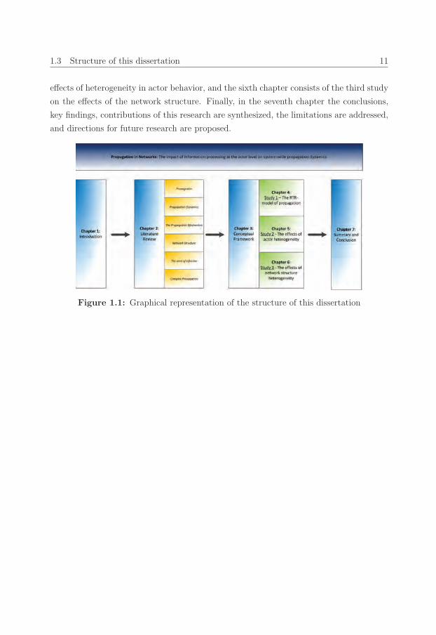
This dissertation consists of seven chapters. This first chapter has introduced the research
topic, focus and research questions. The second chapter consists of a conceptual study,
covering the concepts of propagation, networks and propagation dynamics in more detail.
It will consider existing models of propagation and introduces the model incorporating the
information processing view; the RTR-model of propagation. The third chapter provides
the conceptual framework of this dissertation, introducing three distinct studies, each
covering a chapter. The fourth chapter consist of the first study which focuses on the
effect of differences in the propagation mechanism, the validation of the RTR-model and
showcasing its relevance for interventions. The fifth chapter covers the second study on the
13_Erim_Vermeer Stand.job
1.3 Structure of this dissertation 11
effects of heterogeneity in actor behavior, and the sixth chapter consists of the third study
on the effects of the network structure. Finally, in the seventh chapter the conclusions,
key findings, contributions of this research are synthesized, the limitations are addressed,
and directions for future research are proposed.
Figure 1.1: Graphical representation of the structure of this dissertation

13_Erim_Vermeer Stand.job

14_Erim_Vermeer Stand.job
Chapter 2
The concept of propagation in
networks
This chapter considers the main concepts used in this dissertation: propagation, propa-
gation dynamics, and network structure. Relevant literature is reviewed with respect to
propagation dynamics. The chapter is structured as follows; the first section considers
the concept of propagation and its dynamics. The second section focuses the propagation
mechanism. The third section describes the network structure. The fourth section will fo-
cus on local heterogeneity. The fifth section will consider how these drivers of propagation
interact.
2.1 What is propagation?
The term propagation stems from the Latin word propagat which according to the Oxford
dictionary means ‘multiplied from layers or shoots’, and refers to the process by which
new shoots grow from the parent plant. It hence refers to the process by which the plant
evolves, and extends its presence. Other derivatives of the word propagat are propeller,
which describes the tool used for moving a craft from one location to another, and propa-
ganda, which means ‘that which should move forward’. Both describe something moving
from one location to another.
Similarly the term ‘propagation’ is used to describe the process by which something moves
from one place to another. It is used primarily in physics where, for example, under the
label ‘wave propagation’ it describes the motion of a wave throughout a medium or the
transfer of its energy. Under the label of ‘crack propagation’ it describe the motion of
the crack tip or the crack front during the fracture of materials. As ‘radio propagation’
it refers to the behavior of radio-waves when they are transmitted, or propagated from
14_Erim_Vermeer Stand.job
14 The concept of propagation in networks
one point on the Earth to another. Propagation thus generally refers to a process of
displacement; the spread of something in place and/or time.
The term propagation is not very commonly used outside the field of physics to describe
such spreading processes. Phenomena fitting the description of propagation are however
studied by scholars in many different fields. Throughout literature the propagation pro-
cess has received different names based on the context in which is has been studied. Most
commonly cited notions are those of contagion (of disease) (Dodds and Watts, 2004; Rah-
mandad and Sterman, 2008), social contagion (Burt, 1987; Galaskiewicz and Burt, 1991;
Iyengar et al., 2011; Aral, 2011), social influence (Turner, 1991; Cialdini and Goldstein,
2004; Friedkin, 2006; Ma et al., 2014), cascading process (of disasters) (Buldyrev et al.,
2010; Buzna et al., 2006; Watts and Dodds, 2007), diffusion of innovation (Coleman et al.,
1966; Rogers, 1995; Guler et al., 2002; Valente, 1996, 2005) and information diffusion (Aral
et al., 2007; Reagans and McEvily, 2003). While these notions do differ in the way they
describe propagation, they all describe a process by which interaction among actors causes
some sort of signal to flow from one place or person to another, and hence fit the general
description of propagation.
In describing propagation four basic elements can be identified: a source, a broadcasted
signal, a medium which transports this signal, and a receiver of the signal. For propaga-
tion to occur the sender will broadcast a signal. This signal can be anything ranging from
energy, information, to a change in state or behavior. This signal is then transported
through the medium to another place in the system where it eventually has an effect
on the receiver(s). The labels ‘sender’ and ‘receiver’ indicate that there is some sort of
behavior associated with propagation. While both the sender and receiver are expected
to show behavior or act during propagation, for the purpose of this dissertation they are
referred to as actors. Actors can be anything ranging from molecules, as is the case in the
previously introduced examples of propagation, to people, firms or even species depending
on the granularity of the process considered.
Borgatti (2005) defines propagation as a flow in a network of interacting actors. By doing
so Borgatti (2005) explicitly mentions a network facilitating the propagation process,
effectively stating that the network of interactions serves as the medium for transporting
signals. This work implicitly argues that propagation is a network process, and should be
defined as such. Following this notion, the propagation process is, for the purpose of this
dissertation, defined as:

15_Erim_Vermeer Stand.job
2.1 What is propagation? 15
Definition 2.1. Propagation: The process by which the (change in) state or behavior of
one actor results in a change in state or behavior of one or more of its connected neighbors
As the behavior of neighbors changes this can consequently propagate towards the neigh-
bors’ neighbors, and so on and so forth, until potentially the whole network is affected.
Apart from describing the propagation process as a network process Borgatti (2005) makes
another contribution. In his paper he makes a clear distinction between two types of prop-
agation; on one hand flows that occur in the form of a (physical) transfer from actor to a
connected neighbor (the alter), and on the other hand flows that occur as duplication.
In the case of transfer the original owner is left empty handed after propagation, and
hence the ‘signal’ being propagated is changing physical location, think for example of
moving a box. The box can only be in one location at any time, so in order to move the
box to another location it needs to be removed from the current location.
During duplication this is not the case, here the signal can in fact be at different locations
at a single point in time. Therefore it does not need to leave the point of origin during
propagation. An example of duplication could be knowledge sharing. The knowledge
does not disappear at it’s origin when it is transferred, it remains at the initiator while
the signal (the information regarding this knowledge) moves towards to alter. In turn
this signal can result in the duplication of the behavior or state at the alter, the neighbor
becoming knowledgeable as well.
In this dissertation the focus is on propagation processes which take place by means of
duplication. It aims to understand phenomena which have the potential to cause system
wide change, which can cause emergent behavior. Such changes require large parts of the
system to be affected simultaneously, and therefore consider a process which can have
an effect on multiple actors at the same time. Such a spread throughout the system can
only be achieved by the propagation processes which occur by means of the mechanism
of duplication (Borgatti, 2005).
2.1.1 Propagation of shocks
The definition of propagation adopted is deliberately very broad. Propagation phenom-
ena occur in a wide range of fields, this definition of propagation is designed to fit such a
wide range of settings. It can cover any process in which interaction among actors occurs,
even though not every process is equally relevant to study.
Strictly speaking any actor interaction affects this actor, be it only on a molecular level.

15_Erim_Vermeer Stand.job
16 The concept of propagation in networks
Therefore any interaction is likely to yield some sort of propagation. However not every
interaction will have an impact which is significant. Therefore not all propagation dynam-
ics might be equally relevant to study. For example, in order to understand the emergent
behavior in groups of people it might not be relevant to consider the molecular change
for each person. This suggests that some threshold exists for which kind of propagation
effect should or should not be considered. The choice for such threshold will always be
arbitrary and dependent on the phenomenon being studied, therefore this dissertation
refrains from implementing an explicit threshold.
Rather than implementing a strict threshold or studying all propagation dynamics it will
focus on the propagation of shocks. Note that while a shock has the connotation of being
a negative and harmful event this is not the meaning of a shock in this dissertation. For
the purpose of this dissertation a shock is defined as:
Definition 2.2. A Shock: A rapid, unexpected and large change in the state or behavior
of one or more actors in the network.
In this definition ‘rapid’ implies that the time it takes for the shock to propagate is at
least an order of magnitude smaller than the time it takes actors to strategically absorb
such signals, therefore when considering the propagation of shock the actual propaga-
tion process is separated from strategic behavior actors might have. ‘Unexpected’ implies
that being subject to a specific shock cannot be foreseen by an individual, and hence no
last minute counter-measures can be taken to absorb such a shock. ‘Large’ implies that
the behavior or state of an actor is significantly different than it was prior to the shock.
Based on these characteristics studying propagation of shocks has three advantages; 1)
The effects of shocks are likely to be seen on a relatively short time-span, 2) the effects of
shock propagation are likely to be profound, potentially catastrophic, making the effects
of propagation more easily identifiable and 3) strategic behavior of actors plays no role in
the dynamics of the propagation process in the short term.
2.1.2 Existing models of propagation
Studying shock propagation in a system requires some sort of model to capture the be-
havior of the process. As literature on propagation is quite dispersed across disciplines
this body of work has yielded a wide variety of models. They can be classified into four
main model categories; SIS/SIR models (Kermack and McKendrick, 1927), Bass(-like)
models (Bass, 1969), threshold models (Rogers, 1995; Valente, 1996) and cascade models
(Kempe et al., 2003). A brief description of each of these models is provided below.

16_Erim_Vermeer Stand.job
2.1 What is propagation? 17
SIS/SIR models
By far most models of propagation are based on SIS/SIR type of models. These model
stem from the field of epidemics. They owe their name to the states of actors in the model.
In these models actors are either Susceptible, Infected or Removed, hence resulting name
SIS/SIR model. These models describe the process by which actors are changing from
Susceptible to Infected by means of an infection rate (λ) and a process by which actors
change from Infected to Susceptible/Removed certain recovery rate (ρ) or death rate (γ),
these processes are considered to be stochastic and dependent on the interactions among
actors.
Even though many extensions of the traditional SIR/SIS models exist (most of them add
extra state to the model, for example by allowing actors the be exposed, or temporary
immune) for convenience the simple SIS model will be elaborated in order to introduce
this type of propagation model. In this model the population is divided in different
compartments of actors, each with a different state. These compartments interact at a
certain rate which is based on the size of the population in each of the states available in
the system. By considering the average rates by which the actors change from one state
to another, such models allow writing the dynamics of propagation as a set of differential
equations. Assume a set of N actors which are either susceptible (S) or infected (I) such
that N = S + I. In this case the SIS model is described by:
ΔI
Δt= −ρI +
βSI
N(2.1)
ΔS
Δt= −βSI
N+ ρI (2.2)
In which β is the rate of interaction.
This model assumes random interactions among actors, essentially considering a scenario
with homogenous mixing. More complicated extensions have been developed which in-
clude the notion that there is a network underlying the propagation process. The network
causes actors to have a certain amount of connections, which affects their ability to both in-
fect others, and be infect by others, resulting in the following formulation Pastor-Satorras
and Vespignani (2001a):ΔI
Δt= −ρI + I〈k〉λ(N − I) (2.3)
ΔS
Δt= ρI − I〈k〉λ(N − I) (2.4)
16_Erim_Vermeer Stand.job
18 The concept of propagation in networks
In which 〈k〉 is the average number of edges (connections) per vertex (actor).
A more complex variation of this model can also capture heterogeneity in the network
structure (Pastor-Satorras and Vespignani, 2001a,b). What these models do is assign
actors to a certain group, a compartment, based on their state and number of connections.
It is assumed that all actors in the same compartment behave similarly. This model
leverages the average behavior of actors in a compartment, for this reason it is an example
of a mean-field model. Mean-field models can be roughly divided in three camps (Pastor-
Satorras et al., 2014):
• Individual-based mean-field approach (IBMF): In which it is assumed that every
actor belongs to compartment of the system with a certain probability, and that all
actors within a compartment behave similarly.
• Degree-based mean-field approach (DBMF): Here compartments are based on the
number of ties an actor has. It is assumed that every actor with the same number
of ties, its degree, behaves statistically similar.
• Generating function approach: A special case method for scenarios in which infected
actors are removed after infection. Which builds on the notion that the likelihood
of finding a tie is related to the probability of transmission of the disease, which is
constant for the complete population.
Pastor-Satorras et al. (2014) provide an mathematical representation of these models and
an extensive overview of their characteristics and differences. Each of these approaches
shares the same leveraging mechanism, they consider the propagation behavior averaged
over a groups of actors or the system as a whole. The main argument for doing so is
that this allows these models to step away from the apparent chaotic behavior of the in-
dividual actor level (NWO, 2014). Also combining set of actors, significantly reduces the
complexity of the formulation of the propagation behavior. Because of this these so-called
mean-field approaches enable using an analytical methodology to untangle the propaga-
tion process. This in turn has resulted in closed form solutions to many propagation
problems Pastor-Satorras et al. (2014).
Cascade models
A second type of propagation models is the cascade models (e.g. Goldenberg et al. (2001)).
This type of models similar to the SIS models considers a stochastic process in which an
‘infected’ actor will propagate its behavior towards it connected neighbors. Potentially
resulting in the occurrence of cascades of such behavior. An important characteristic of

17_Erim_Vermeer Stand.job
2.1 What is propagation? 19
cascade models is that they are build on the notion of momentum. This means that once
an actor changes state, it will sent out a signal towards a neighbor only once! Regardless
of this result of the consequent propagation process it loses its momentum after this initial
shock and will become inactive as a result.
As Kempe et al. (2003) puts it ‘The basic cascade model therefore can be described by
a process which starts with an initial set of active I0 actors. The propagation process
unfolds in discrete steps according to the following randomized rule. When node i first
becomes active in time step t, it is given a single chance to activate each currently inactive
neighbor j; it succeeds with a probability pi,j —a system-wide parameter— independently
of the history thus far ’.
Threshold models
The third type of propagation models, the threshold models (e.g. (Valente, 1996)) assume
a different type of propagation mechanism. These models assume that adoption of a
certain state is a consequence of the states of its connected neighbors. In each time step
all actors will therefore reconsider their state. Each actor will look at its direct neighbors
and change state if a large enough proportion of the neighbors has adopted an alternative
state. Whether the proportion of the neighbors is big enough to change state, depends
on the adoption threshold of the focal actor.
Kleinberg (2007) describe the most basic threshold model, the linear threshold model,
in which it is assumed that each actors has an individual threshold for changing its
behavior. For each actor the proportion of neighbors needed differs, the threshold is
chosen randomly. The model consists of two elements:
• A set of edges E with a positive weight wij on each edge from i to j, which indicates
the influence of actor i on j . It is dictated that∑
w∈N(j) wij ≤ 1 , where N(j) is
the set of nodes with edges to j.
• A set of thresholds Θ, containing a threshold θi for each node i. θi is chosen uniformly
at random from [0, 1]
Due to some external event a set of nodes will initially adopt the alternate behavior, these
nodes are claimed to be active. At any discrete time step t = 1, 2, 3, . . . any inactive node
j becomes active if the fraction of active neighbors exceeds its threshold:
∑A∈N(j)
wij ≥ θj (2.5)
17_Erim_Vermeer Stand.job
20 The concept of propagation in networks
Where A is the set of active nodes. While far more complicated threshold models can be
considered, for example by considering also the absolute number of neighbors (Kleinberg,
2007; Centola and Macy, 2007) all threshold models follow this fundamental mechanism
of updating the state of actors based on the state of the connected neighbors.
Bass-like models
The traditional Bass model (Bass, 1969) was used to describe the adoption of innovation
among actors. It consists of a differential equation describing the process of how such
adoption occurs. The basic premise of the model is that adoption is driven by two forces,
random adoptions, and influence from other actors. Each actor is classified as innovator
or as imitator. Innovators are those which have a high probability to adopt a innovation
at random, and imitators are those which are more likely to adopt due to influence. The
speed and timing of adoption depends on their degree of innovativeness and the degree of
imitation among adopters.
The basic Bass model is formulated as:
f(t)
1− F (t)= p+ qF (t) (2.6)
In which f(t) is the change in the proportion of adopters, F (t) is the proportion of
adopters, p is the rate of innovation (random adoption) and q is the rate of imitation.
The Bass model can also be written as a discrete time model (Lilien et al., 2000), in which
case it is formulated as:
x(t) =
[p+ q(
X(t− 1)
m)
][m−X(t− 1)] (2.7)
In which x(t) is the number of adopters at time t, X(t − 1) is the cumulative adopters
before time t, p is the coefficient of innovation, q is the coefficient of imitation and m
is the number of eventual adopters. This version of the model has been extended to
the generalized bass model (Bass, 1994), which captures the effect of marketing effort by
including a multiplication factor Z(t). resulting in the following formulation:
x(t) =
[p+ q(
X(t− 1)
m)
][m−X(t− 1)]Z(t) (2.8)
In which Z(t) is oparationalized as:
Z(t) = 1 +α [P (t)− P (t− 1)]
P (t− 1)+ βmax
{0,
[A(t)− A(t− 1)]
A(t− 1)
}(2.9)
18_Erim_Vermeer Stand.job
2.1 What is propagation? 21
In which α is the coefficient for increase in diffusion due to price decrease, P (t) is the
price at time t, β is the coefficient for increase in diffusion due to marketing, and A(t)
is the advertising at time t. Again, many other variations of the Bass model have been
proposed, but the overall form and dynamics remain the same. All these variation propose
some way in which the initial bass model will be perturbed, and hence can be seen as
models in which the operationalization of Z(t) is changed.
It should be noted that the Bass model does not mention a structure of interactions,
and hence this model ignores the impact of the network structure. It effectively assumes
that actors have full information on the state (changes) of actors in the system, which
can be translated into assuming a completely connected network, in which each actor is
connected to each other actor.
2.1.3 Propagation dynamics
Describing the propagation of shocks highlights the potential of propagation to quickly
spread among actors before for strategic action can be taken that absorbs the effects of
the propagation. Consequently shock propagation processes have the potential to affect
large parts of a system, which can consequently destabilize the system. Following this
line of reasoning most models of propagation have adopted a perspective of measuring
the impact of a propagation process on the system level. It should however be noted
that propagation outcomes do not necessarily need to be considered on the system level.
Especially in the process of scaling up, while propagation is turning into a global cascade,
the outcomes might be interesting to consider. This suggest that, rather than capturing
the propagation outcomes at a specific point in time, the timing/stage of propagation
outcomes should be considered. Therefore for the purpose of this dissertation will be
referred to propagation dynamics, which capture the propagation outcomes and their
evolution in time. The propagation dynamics are defined as:
Definition 2.3. Propagation dynamics: The outcomes of propagation over a certain
period of time, in a pre-defined part of the system.
This definition suggest that not only the timing, and evolution of the outcomes are crit-
ical, but also that location which is considered matters. While, in theory, any arbitrary
part of the system could be selected, selections are often in one of three levels: Micro-, the
meso- or the macro-level. The micro-level consider a dynamics in a dyad, the meso-level
considers how it grows towards a sub-set of the network —a cluster or quadrant—, and

18_Erim_Vermeer Stand.job
22 The concept of propagation in networks
the macro-level (also called the system-level) considers the system as a whole.
Propagation dynamics not only capture how neighbors affect one another, but also how
the system is affected, which actors in a system are impacted, and where such impact
came from. Capturing the full complexity of the propagation dynamics therefore requires
all three levels to be incorporated. However, such a multi-level notion of propagation
dynamics makes it a lot harder to strictly define the dynamics. Therefore often a pre-
defined choice is made on the level at which the dynamics are considered. This choice
will be strongly driven by the research question(s) one wants to answer. To provide a
comprehensive understanding of the different levels of dynamics the following sections will
provide an overview of the levels at which propagation dynamics can be captured.
Propagation dynamics at the micro-level
The definition of propagation describes it as a process which takes place between actors,
it’s dynamics therefore by definition occur at the micro-level. The propagation dynamics
on the micro-level should not be mistaken for the propagation mechanism. The local
dynamics describes whether propagation has occurred between actors. The propagation
mechanism in contrast describes how such dynamics are realized. The dynamics are thus
the result stemming from the mechanism.
The local propagation dynamics have received relatively little attention in literature.
Often it is assumed that there is a single rate or probability, be it the likelihood of trans-
mission, the chance of adoption, the percolation probability or the rate of spreading.
This simple notion might very well explain why local dynamics have received relatively
little attention in propagation literature, there is simply not much to study about a sin-
gle parameter. While processes can vary in the extend to which local dynamics occur,
little is known about why such heterogeneity in dynamics occurs. Describing the local
dynamics using a single parameter obscures the impact of differences in the mechanism
of propagation. In this dissertation it is argued that these differences play a critical role
in determining the local dynamics, suggesting that more complex view of local dynamics
is required. In section 2.3 therefore a nuanced view of the propagation mechanism will be
introduced.
19_Erim_Vermeer Stand.job
2.1 What is propagation? 23
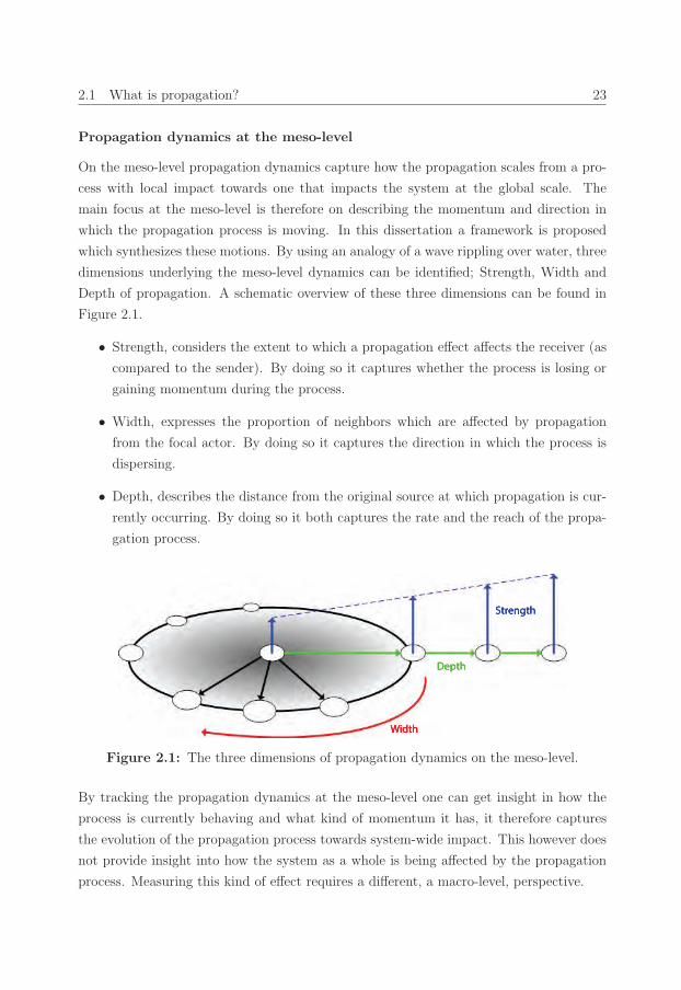
Propagation dynamics at the meso-level
On the meso-level propagation dynamics capture how the propagation scales from a pro-
cess with local impact towards one that impacts the system at the global scale. The
main focus at the meso-level is therefore on describing the momentum and direction in
which the propagation process is moving. In this dissertation a framework is proposed
which synthesizes these motions. By using an analogy of a wave rippling over water, three
dimensions underlying the meso-level dynamics can be identified; Strength, Width and
Depth of propagation. A schematic overview of these three dimensions can be found in
Figure 2.1.
• Strength, considers the extent to which a propagation effect affects the receiver (as
compared to the sender). By doing so it captures whether the process is losing or
gaining momentum during the process.
• Width, expresses the proportion of neighbors which are affected by propagation
from the focal actor. By doing so it captures the direction in which the process is
dispersing.
• Depth, describes the distance from the original source at which propagation is cur-
rently occurring. By doing so it both captures the rate and the reach of the propa-
gation process.
Figure 2.1: The three dimensions of propagation dynamics on the meso-level.
By tracking the propagation dynamics at the meso-level one can get insight in how the
process is currently behaving and what kind of momentum it has, it therefore captures
the evolution of the propagation process towards system-wide impact. This however does
not provide insight into how the system as a whole is being affected by the propagation
process. Measuring this kind of effect requires a different, a macro-level, perspective.
19_Erim_Vermeer Stand.job
24 The concept of propagation in networks
Propagation dynamics at the macro-level
Macro-level propagation dynamics capture the effect of the propagation process at the
system level. The system-wide impact of propagation has received by far the most at-
tention in literature. Therefore, there are quite some explicit measures capturing the
macro-level propagation dynamics. These measures can be divided into three main cate-
gories; impact, speed and location.
Impact
The impact of propagation has obtained by far the most attention in literature. All pre-
viously introduced models aim at specifying the proportion of the population which is
infected, essentially capturing the impact of the propagation process at the system level.
The population of infected actors, the so-called prevalence (Pastor-Satorras and Vespig-
nani, 2001a), is a dominant measure of describing the impact of propagation at the system
level. It should be noted the prevalence of a process varies over time. In scenarios with an
recovery process this results in a basin of attraction(s) for the process. At some point the
number of newly infected actors, offsets the number of newly dis-infected actors, resulting
in an (dynamic) equilibrium at the system level. The prevalence in this (semi)stable state,
can be either positive or zero, indicating whether a propagation process in the long run
is viable from prevailing in a population.
Speed
In scenarios without a recovery process there will be no new dis-infections, therefore such
equilibrium state will not be present. Consequently rather than studying the extent of
impact at any given stage in the process, often the speed by which it occurs is considered.
The prime interest is on the time it takes for a process to reach (an arbitrary) critical
mass, for example the time it takes for the 90% of the population to become infected.
Location
The last category of macro-level propagation dynamics measures focuses at the location of
the propagation effects. The primarily aim for such measures is describing which part(s)
of the network are affected (most). Here the system is divided into different sparsely
connected groups, clusters, and one considers which clusters are affected and which ones
are not.
The categories of system-wide propagation dimensions are not mutually exclusive; hybrid
metrics can occur, and are receiving increasing amount of attention. An example of
a hybrid method which has seen increasing use (e.g. (Stonedahl et al., 2010; Peres,
2014)) is the net present value (NPV) method put forward by Goldenberg et al. (2007).
By assigning a value to each adoption and making this value time dependent —longer
20_Erim_Vermeer Stand.job
2.1 What is propagation? 25
adoption times yield diminishing gains— elements of both the impact and the speed are
combined into a single measure.
2.1.4 Three drivers of propagation dynamics
Propagation literature has provided limited insight in what causes propagation dynamics.
Generally variations in the propagation dynamics are attributed to one (or more) of three
drivers:
• The starting point of the propagation process, the seed of the infection
• The process by which the behavior spreads between actors, the mechanism of prop-
agation
• The structure of interactions in the population, the network structure
When considering the definition of propagation used in this dissertation, one can observe
that each of these drivers is represented.
First, the ‘connected neighbors ’ part of the definition links to the network structure. Hav-
ing connected neighbors implies some sort of connection among actors. An overview of
these connections can be represented in a network or graph, in which the actors are nodes
and the connections are edges. The resulting network graph depicts the structure of
interactions, which serves as the medium facilitating propagation. As this medium is a
necessity for propagation, the network structure capturing this medium provides a bound-
ary condition for propagation, which will consequently affect propagation dynamics.
Second, the definition mentions ‘the (change in) state or behavior of one actor ’, which
can be linked to the seed of infection. Although the definition considers the starting point
of the dyadic process and the seed of infection refers to the start of the process as a whole,
both suggest that there is a source of propagation. Linking the dyadic starting point to
the process as a whole implies taking into consideration the network structure beyond the
dyad. The inherent heterogeneity of these structures, is what makes the seed a crucial
aspect in system-wide propagation dynamics. Having heterogeneous network structures
means that the structure within a network will vary locally, and will be different de-
pending on which part of the network is considered. As this local structure provides the
infrastructure which can be leveraged the early stage of the propagation process it will
determine the ability for the propagation process to gain critical mass and momentum.
As the seed in turn dictates which local structure will be available this seed can strongly
influence the process dynamics.
Third, the definition of propagation mentions ‘The process by which’ which directly links
20_Erim_Vermeer Stand.job
26 The concept of propagation in networks
to the mechanism of propagation. While the definition does mention the mechanism of
propagation, it does so on a high level of abstraction. It does not specify any character-
istics of the mechanism, fundamentally treating the mechanism as a black box.
Each of these drivers seems to capture part of what constitutes propagation dynamics,
therefore in the following sections each of the drivers will be considered in more detail.
2.2 The propagation mechanism
The notion that the mechanism of propagation is a driver of propagation dynamics has
received relatively little attention in propagation literature. It is widely accepted that
there is an effect of the mechanism, however this effect is often not explicitly mentioned.
It has been recognized that models adopting different description of the propagation pro-
cess, a different mechanism, can yield different propagation dynamics (Rahmandad and
Sterman, 2008), yet the impact of the mechanism has to my knowledge not systematically
been studied.
The lack of emphasis on the impact of the mechanism might, in part, be due to the design
of mainstream propagation models. It seems intuitive to assume that some processes are
more effective than others, and that consequently the way in which one actor affect its
neighbor(s) will vary across processes. In line with this logic mainstream propagation
models have captured and parameterized the local propagation dynamics, the extend to
which propagation among actor occurs successfully. All mainstream models describe a
certain rate or probability success —be it the likelihood of transmission, the threshold for
adoption, the percolation probability or the rate of spreading— and therefore incorporate
and parametrize the local dynamics of propagation. They however also ignore the mech-
anism by which such dynamics are caused.
Doing so allows for reducing the complexity of propagation models, as local dynamics can
be captured using a single parameter. Which has resulted in the conclusion that variation
in such a parameter yield very different behavior on the macro-level (Pastor-Satorras and
Vespignani, 2001a). However, it also significantly reduces the extent to which one can
make claims regarding the impact of the process itself. When a single parameter is used
to describe a complex process little detail can be captured, and little insight can be gained
on the impact of the process itself. Hence the quest for simplification migth very well be
the reason why differences in the mechanism have received little attention in propagation

21_Erim_Vermeer Stand.job
2.2 The propagation mechanism 27
literature.
Building on management literature it is argued that this lack of emphasis might pose a
problem. A commonly accepted notion in management literature, especially in the field
of (business) process management (e.g. (Becker and Kahn, 2003; van der Aalst et al.,
2003)), is that outcomes in organizations are the result of an underlying (production)
process. It is argued that the best way to improve organizational outcomes is to stream-
line this process. However, in order to streamline the process there needs to be insight into
the mechanism by which this process takes place. Therefore this body of management
literature implicitly suggests that understanding the underlying mechanism is critical in
order to effectively steer and manage its outcomes. In this dissertation a similar argument
is made for the propagation process, it is suggested that in order to steer and manage
propagation outcomes, its dynamics, one needs to be able to understand and describe the
mechanism by which the process occurs.
2.2.1 The propagation mechanism in practice
The definition of propagation captures the propagation process at a high level, without ex-
plicitly characterizing the mechanism which makes up this process, effectively considering
the mechanism of propagation to be a black box. While this allows for combining termi-
nologies and capturing practical phenomena across different setting, it has little value in
terms of understanding the effects of the mechanism. In order to make sensible claims
about the effects of the mechanism one needs to open the black box of propagation and
provide a detailed description of what happens during the process.
The best way to get a grasp of what happens during propagation is to observe and describe
how this phenomena occurs in practice. Propagation phenomena occur in many different
fields, which provide a rich source of potential insights. As links between these fields
are not necessary strong, it is expected that each setting can yield different insights into
the propagation mechanism. Therefore, to explore the behavior during the propagation
process a set of six practical propagation phenomena is considered; the spread of influenza,
giving a political speech, spreed of financial crisis, a cascade of breakdowns, diffusion of
innovation and knowledge sharing.
21_Erim_Vermeer Stand.job
28 The concept of propagation in networks
Propagation in biology - The spread of influenza
The propagation of influenza starts with one (or more) infected individuals. These indi-
viduals start spreading germs by air by means of a sneeze. During the sneeze an actor
sends out a signal, it releases germs into the air. Note that the number of germs send
out during the sneeze, is not necessarily the same as the number which reaches an alter.
There will be a certain dispersion of germs which causes the number of germs which reach
the alters to be dependent on for example the proximity between actors. while germs
reaching an alter is a necessary condition for infection, the alter getting sick will depend
on how this alter responds to the germs which reach him/her. The immune system and
the resistance of the alter will play a crucial role in determining how this signal (germs
which reach the alter) will lead to him/her becoming sick.
Clearly, for influenza to spread a sneeze of the focal actor is not sufficient. Germs will
need to travel from the sender to his/her alters, and these alters will need to respond to
those germs by becoming sick. This indicates that the spread of influenza takes place in
three consecutive steps.
Propagation in sociology - Giving a political speech
In a political speech a speaker aims to convey his/her standpoint to the crowd and con-
vince them to change their standpoint. The behavior which is propagating is therefore
the standpoint on a certain matter. This is propagated by sending words (actually sound-
waves) towards the crowd. While this signal sent is singular, the manner in which it
is received can vary based on the receiver, volume and clarity can vary across different
locations at which alters are located. Even when the sounds reaches the alter in a sim-
ilar manner this signal can be interpreted very different among alters. Messages bear a
certain meaning, the extent to which such meaning will be deduced strongly depends on
the understanding of the recipient. Understanding a message still is no guarantee the
alter will change it standpoint, the interpretation and existing social context will affect
the alters response to the new information.
Giving a political speech is a good example of a phenomena which captures social conta-
gion. This process has many similarities to the mechanism observed in the contagion of
disease; a signal is sent, transmitted and received. The main difference however lays the
fact that there is a social context in which signals are received. While in disease spreading
the signal being received (number of germs/virus load) is a tangible (although very small),
in scenarios of social contagion this is not the case. This requires an additional step of
22_Erim_Vermeer Stand.job
2.2 The propagation mechanism 29
sense-making while processing signals.
Propagation in economics - Spread of the financial crisis
The financial crisis has recently received a lot of attention of scholars. It is often claimed
to be a contagious process; A financial institution becomes insolvent (due to some external
circumstance) and hence is legally required to obtain additional funds. It can do so by
selling fixed assets, borrowing additional money or defaulting on a loan. Each scenario
will be briefly considered.
In the first scenario, selling fixed assets, the distressed institution has to take a haircut
due to the fire-sale of the fixed assets (accepting a lower sale-price for the fixed asset to
liquidate it), effectively reducing the value and market price of that asset. While other
financial institutions are likely to have some overlap in assets, such price drops can affect
the financial status of these institutions. The market-mechanism in this scenario allows
the behavior of the distressed actor (selling fixed assets) to affect the financial state of
other actors in the system, which in turn can also become distressed.
In the second scenario, borrowing additional money, the propagation effect is two-fold; not
only will the distressed institution (attempt to) borrow additional money, and by doing so
send a direct signal to the counterpart of this transaction. Also the market for obtaining
loans can be affected similar to the sales of fixed assets. As the distressed institution needs
to fulfill its solvency criteria, it will be willing to incur additional costs for obtaining the
required money (similar as in the case of haircuts) hence interest can increase. Again
such increase in interest can influence the market price on loans, effectively affecting
other institutions willingness to borrow/lend. This mechanism is what led to a liquidity
freeze in the financial system in which institutions where unwilling to borrow/lend money
to/from one another.
In the third scenario, defaulting on a loan, the focal firm lets the counterpart of the
loan know that it is in a distressed state. Not only can this information become public
indicating that there is an increased risk of transacting with this specific institution. Also,
the counterpart of the loan is directly affected by the fact that it will not receive a the
prospected income from this loan, directly affecting the financial status of this institution.
Often the three scenarios go hand in hand when a financial institution is distressed, this
makes propagation of the financial crisis in practice a complex matter to study.
While the details of each scenario differ in them three steps in the propagation mechanism
can be identified. The distressed state of an institution results in it behaving out of the
ordinary (sending out a signal), which reaches the alters (either directly or by means

22_Erim_Vermeer Stand.job
30 The concept of propagation in networks
of market mechanism), changes their financial state and can in turn render them in a
distressed state. This setting is different in the sense that little processing of the signal
during reception occurs, there simply is a change in the financial state, whether this makes
the institution distressed depends on the existing financial status.
Propagation in engineering - Cascades of breakdown
An example of transport of energy is used to illustrate the cascade of breakdown. In this
setting the network is used to transport current, which suggest a transport of physical
matter, which by definition is bound by a location. This would suggest that propagation
can only occur at one place at a time. It should however be noted that the behavior which
is claimed to propagate is a form of breakdown. While such breakdowns are caused by
the physical flow previously described, they are not bound to a single location and can
occur at multiple places at once.
Consider the breakdown of a power station (due to some external event). As physical
flows still need to occur in the network the system will attempt to reroute flows to remain
maximally operational. this rerouting changes the remaining flows, which will affect the
load at other stations, potentially causing them to overload and consequently break down.
Again three steps in the mechanism of propagation can be identified. An station breaks
down and stops processing the flow of current, the flows are redirected via other stations,
which in turn are faced with a changed load, which might result in them becoming over-
loaded. This setting is different in the sense that the (change in) physical flow serves as
the medium which allows a breakdown to be transferred to the alters.
Propagation in business - Diffusion of innovation
Diffusion of innovation/information is initiated by an actor (a firm or individual) adopt-
ing or developing an innovation or a piece of information. Information with regards to
this adoption starts being sent out either voluntarily, the actor talks about the innova-
tion/information, or involuntarily, when the adopter starts behaving observably different.
By means of interaction other actors in the system will be able to observe this behavior,
interpreting this as a signal of adoption. After being subject to such a signal the alter
then has to respond by either adopting or not adopting the innovation/information itself.
This scenario again clearly identifies three steps in the propagation mechanism. It is inter-
esting to note that the transport of the adoption signal in this setting can both be caused
by a push mechanism, in which case it is initiated by the adopter, and pull mechanism in
which case it is initiated by the alter.

23_Erim_Vermeer Stand.job
2.2 The propagation mechanism 31
Propagation in management - Knowledge sharing
Knowledge sharing is a prime example of how propagation is considered in management.
In order to map how groups of people behave and learn —be it teams or the organization
as a whole— managers have tried to understand how knowledge is shared within (and
between) groups. In this process there is commonly an individual who possesses the
desired knowledge, this actor can be considered as the starting point of the propagation
process. This actor communicates with the remainder of the group, by means of various
communication media, allowing a flow between these individuals to occur. While this
indicates that something can be shared, it is not knowledge which is flowing between
them, the knowledge sharing process is slightly more complicated. Knowledge only exists
as an interpretation of information. Therefore, a knowledgeable actor can share with
its alters information (a codification of his/her knowledge), but not knowledge in itself.
Similarly alters can receive information, but this information needs to be interpreted in
order to result in (propagated) knowledge. Knowledge sharing therefore explicitly requires
a flow of information but also actors to code and decode information. The extent to which
this will effectively occur strongly depends on the capabilities of both sender and receiver.
2.2.2 The information processing view of propagation
In the real world examples of propagation two important characteristic of the propaga-
tion mechanism can be observed. First, the behavior which is propagating can be very
different from the signal which is flowing between actors. And Second, the mechanism of
propagation seems to be taking place in a structure with remarkably steps.
In many of the examples of propagation in the previous section a signal which is actually
flowing between actors can be observed. To convince someone of a standpoint (which is
the behavior that propagates) actors send out sound-waves, cascades of failures propagate
by means of a changing current or load in the network, and spread of innovations and
knowledge required a flow of information. This indicates that a ‘signal’ is transferred
during propagation. This signal is often not the same as state or behavior which is prop-
agating. Instead the signal captures some form of information regarding the state or a
change in the state. This suggest that propagation is at its core a process by which an
information signal is processed.
The real world propagation phenomena also appear to have significant overlap in their
mechanism. Each process describes three distinct steps; An actor sends out a signal, this

23_Erim_Vermeer Stand.job
32 The concept of propagation in networks
signal reaches one or more alters and the alter(s) process the signal by (not) changing
their state accordingly. This observation is in line with communication theory (Shannon,
1948), which is known for describing the information processing process, which similarly
captures these three steps.
Based on these observations it is argued that the propagation process can be considered as
an information processing process, and capturing this notion the information processing
view of propagation is put forward. This view considers the propagation process to consist
of three subsequent sub-processes by which an information signals flow between actors
and consequently behavior/states can propagate. Rather than considering one overarching
process and describing it propagation dynamics, this view describes the mechanism during
propagation by which these dynamics occur.
2.2.2.1 Three sub-processes of propagation
All propagation processes require some sort of trigger, something which makes one actor
change state, and consequently act as the seed of the propagation process. The initial
change in state is considered to be due to some arbitrary external event. Due to this
event the focal actor will change its state and starts affecting its alters. It will do so by
sending out information regarding the (change in) state/behavior to those with whom
it is interacting. This can be done by broadcasting this information, effectively sending
a signal towards neighbors in all directions, or by narrow-casting, providing this infor-
mation to a specific subset of neighbors. Because signals can be sent in many different
directions this sub-process of propagation is referred to as the Radiation. Note that ra-
diation links directly to the width dimension of propagation dynamics introduced in the
previous section. Furthermore, radiation implies that information can be duplicated and
sent in multiple directions, therefore it fits perfectly with the duplication Borgatti (2005)
notion of propagation.
The next step that needs to be taken is that the ‘radiated’ signal needs to be transported
from the focal actor to its neighbor(s). Think of this as sending a pulse over a wire;
The pulse which is sent is not necessarily the same as the one which reaches the end of
the wire, some loss or distortion can occur during this process. Similarly the during the
transport the propagation signal distortion can occur, some part of the information might
be lost or altered, communication theory refers to this as noise. The second sub-process
of propagation, the process of transporting the signal over a tie (edge), is referred to as
transmission.
The third step in the propagation process is referred to the as reception sub-process, it
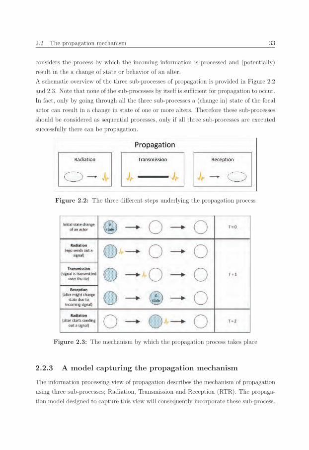
24_Erim_Vermeer Stand.job
2.2 The propagation mechanism 33
considers the process by which the incoming information is processed and (potentially)
result in the a change of state or behavior of an alter.
A schematic overview of the three sub-processes of propagation is provided in Figure 2.2
and 2.3. Note that none of the sub-processes by itself is sufficient for propagation to occur.
In fact, only by going through all the three sub-processes a (change in) state of the focal
actor can result in a change in state of one or more alters. Therefore these sub-processes
should be considered as sequential processes, only if all three sub-processes are executed
successfully there can be propagation.
Figure 2.2: The three different steps underlying the propagation process
Figure 2.3: The mechanism by which the propagation process takes place
2.2.3 A model capturing the propagation mechanism
The information processing view of propagation describes the mechanism of propagation
using three sub-processes; Radiation, Transmission and Reception (RTR). The propaga-
tion model designed to capture this view will consequently incorporate these sub-process.

24_Erim_Vermeer Stand.job
34 The concept of propagation in networks
Based on the names of these sub-processes this new model is labeled the RTR-model of
propagation.
This model introduces three parameter-sets, one for each sub-process. In combination,
these parameters describes the propagation mechanism. These three parameter-sets are
claimed to each be embedded in a separate function, each of which describes a single sub-
process of propagation. The RTR-model of propagation in its most generic form therefore
consists of three distinct functions:
1. a Radiation function
2. a Transmission function
3. a Reception function
This model assumes that there exists an underlying network structure on which the prop-
agation process will take place. This network structure can be considered as a graph
G = (V,E) with vertices i ∈ V := {1, . . . , n} and an edgeset e ∈ E := {1, . . . ,m}. All
edges are assumed to be directed and weighted, where wij,t denotes the weight of the edge
from vertex i to vertex jon time t, and [Wt] is the matrix containing all edge weights
on time t. All vertices i at any point in time have a state si,t, and [St] is the matrix
containing the state all actors at time t (si,t ∈ [St]). The starting state of the system can
thus be denoted as [W0] and [S0], this starting state is assumed to be stable.
The definition of propagation used in this dissertation considers it to be a process which
is initiated by the change in the state/behavior of a seed, one or more actors which change
state due to some external event. It can be measured by a change in the state of a set of ac-
tors on time t = 0, and hence a change in the starting state ΔS0 (ΔS0 = (Δs1,0, ...,Δsn,0)).
This perturbation in turn can result in propagation and consequently destabilize the sys-
tem. The term propagation is only used when the state of vertex set V changes during a
single time-step in the model (St �= St+1).
The propagation process is assumed to take place in discrete time. In every time unit
(t → t+1) the three aforementioned sub-processes occur. First a change in the state of an
vertex i will be sent to the outgoing edges of this vertex in the form of a signal (radiation),
second this signal will be transferred over the edge towards the alter (j) (transmission),
and third the incoming signal(s) will reach alter j and (potentially) result in a change in
the state of the alter j (reception).
25_Erim_Vermeer Stand.job
2.2 The propagation mechanism 35
The radiation sub-process
The radiation function describes how a change in the state of a vertex i (Δsi,t) results in
signal being sent out towards the outgoing edges of that vertex at time t (Eouti,t ⊂ E|wij,t >
0), it can therefore generally be described by:
Δsi,t =∑
e∈Eouti,t
αi,e,t × pouti,e,t =∑
Ai,t × P outi,t (2.10)
In which Ai,t is a vector of radiation parameters (αi,e,t) of actor i at time t towards
its outgoing edges (e ∈ Eouti,t ) at time t (Ai,t = (αi,e,t)|e ∈ Eout
i,t ), and P outi,t is a vec-
tor containing the signals sent from vertex i to all outgoing edges (Eouti,t ) at time t
(P outi,t = (pouti,e,t)|e ∈ Eout
i,t ). The radiation parameters (αi,t) can be influenced by many
aspects, it makes sense to consider it as a function of a set of actor specific characteristics,
which can consequently amplify or dampen the extent to which a change in state results
in radiation.
One should note that this formulation assumes that a change in state results in a signal
only in the consecutive time unit, and consequently the model considers only the cur-
rent changes in state and has no memory of what has happened in previous time units.
Following the notion put forward in previous work (Dodds and Watts, 2004, 2005) the
generalized radiation process can be rewritten to also include memory in the system, ef-
fectively stating that a change in state can have an effect beyond the consecutive time
unit.
Δsi,t =t∑
t′=t−Trad+1
∑(Ai,t′ × P out
i,t′ × (τrad)(t−t′)+1) (2.11)
In which Trad is the memory duration for radiation, the number of time units that a
change in state will yield signals (Trad ∈ {1, . . . , t}). And τrad is the memory inflation
factor for radiation, the extent to which previous signals are remembered. The memory
inflation factor can in theory have any positive value; although values ranging between 0
and 1 are most likely as they refer to a process in which signals are forgotten over time.
Values of τrad higher than 1 suggest that signals have an increasing effect over time, and
hence the effect of a change in state will be amplified over time.
This formulation has some build in boundary conditions; it assumes that any fluctuation
in the state of i will fully radiate into one (or more) signals to the outgoing edges. As in
many propagation models the vertices refer to social entities (which in itself are complex
system with some inherent buffering capacity) it can be argued that vertices have some

25_Erim_Vermeer Stand.job
36 The concept of propagation in networks
absorptive capacity for changes in state. Therefore the assumption that all changes in
state will result in radiation might be too strict to capture real-life radiation dynamics.
In order to make the model more generally applicable the model should able to capture
the notion that there can be some absorption in the system. This is done by stating that
only if a change in state is large enough to pass the radiation threshold u (Δsi,t ≥ u)
there will be any radiation. Including this notion into equation 2.11 yields:
t∑t′=t−Trad+1
∑(Ai,t′ × P out
i,t′ × (τrad)(t−t′)+1) =
⎧⎨⎩Δsi,t if Δsi,t ≥ u
0 if Δsi,t < u(2.12)
In which the radiation threshold (u) can have any positive value. Equation 2.12 describes
the radiation sub-process in its most generic form. However radiation alone is not sufficient
to model the propagation process. In order to model the propagation process both the
other sub-processes (transmission and reception) need to be defined; therefore in the next
section the transmission process will be considered.
The transmission sub-process
The second sub-process of propagation, the transmission process, considers how the signal
coming from a vertex (i) is transmitted over an edge towards an alter (j). This process
can therefore be formulated as follows:
pouti,e,t = φe,t × pine,j,t (2.13)
In which pine,j,t is the signal coming from edge e arriving at alter j at time t, and φe,t is
the transmission parameter of edge e on time t. Similarly to the radiation parameter, the
transmission parameter (φe,t)can be considered as a function of edge characteristic which
influence transmission.
It has been assumed that an edge also has a memory. When referring to an edge memory
cannot occur due to abortive behavior (an edge does not describe an entity but a medium
and hence cannot act or absorb) there can however be a certain capacity in for the medium.
It can be best described by assuming an edge to be a pipeline which has a certain capacity
to transport signals. If a signal does not get transported in a previous time unit, the signal
should go somewhere. It can be assumed that it disappears (no memory), alternatively one
can assume that it (partially) remains in the pipeline. This suggests that the transmission
capacity at time t is influenced by previous signals. Including this notion of memory in
the transmission sub-process yields:
26_Erim_Vermeer Stand.job
2.2 The propagation mechanism 37
pouti,e,t =t∑
t′=t−Ttra+1
(φe,t′ × pine,j,t′ × (τtra)(t−t′)+1) (2.14)
In which Ttra is the memory duration for transmission, and τtra is the memory inflation
factor for transmission. Most existing propagation models do not describe the transmis-
sion process and hence implicitly assume a special case in which transmission has no
effects (φ = 1, Ttra = 1 and τtra = 1). While this assumption in many cases makes sense,
in this dissertation transmission is described in this more generic form for two reasons.
First, it allows for capturing the effects where the transmission does causes signals to
be dampened (or amplified), think for example of the inclusion of noise in communica-
tion, the notion of package loss in IT networks or the notion of resistive losses in power
transport. Second, this formulation allows for easily incorporating the (potential) effects
of edge-weights in the propagation model. The edge weights can be easily included in
the transmission parameter φe,t hence this generic form allows for studying propagation
also in weighted networks, something which is more difficult in traditional propagation
models.
Equation 2.14 describes the generic formulation of the transmission sub-process, however
for propagation to occur still the reception needs to be considered; this is being doing in
the following section.
The reception sub-process
The third sub process of propagation, the reception process, describes how incoming
signals translate into a change in the state of a vertex, in its simplest form it could be
formulated as:
ηj,t ×∑e∈Ein
j,t
(pine,j,t) = sj,(t+1) − sj,t (2.15)
In which ηj,t is the reception parameter considering vertex specific attributes influencing
the reception process of vertex j on time t, and Einj,t is the set of incoming edges to actor j
on time t. Note that this way of modeling assumes that all incoming signals are combined
and have one single parallel effect on a vertex. This formulation therefore assumes that
there is no discrimination on sources of a signal, a claim which especially in social systems
might be dubious. Formulating the generic form of the RTR propagation model therefore
requires a slightly more complex formulation. Consider a vector Ψj,t which contains a set
of ηj,t for each incoming edge (Ψj,t = (ηe,j,t)|e ∈ Einj,t), in which all reception parameters
26_Erim_Vermeer Stand.job
38 The concept of propagation in networks
(ηe,j,t) are dependent on the source, the edge, where the signal is coming from. This would
yield the following formulation for reception:
∑(P in
j,t ×Ψj,t) = sj,(t+1) − sj,t = Δsj,t (2.16)
In which P inj,t is a vector containing all the signals of all incoming ties of actor j at time t
(P inj,t = (pine,j,t)|e ∈ Ein
j,t). Note that while this model assumes that incoming signal can be
added up, however more complex function of aggregating the incoming signals could be
used if one has indications that the process being studied has some none-linear dynamics.
Also note that this formulation assumes that signals are processed simultaneously, rather
than in sequence.
The RTR-model assumes that aggregated signals have one single combined effect on a
vertex per time unit. One could make time units infinity small and thus allow actors
to respond to (and send out) signals sequentially (rather then in parallel). This is for
example done when considering the propagation process as a Markov-chain. Such an
approach is however undesirable for three reasons:
• Processing signals sequentially requires an additional set of assumptions; it requires
requires a very clear set of assumptions on the sequencing of signals (which in itself
is so complex that the treatment is worse than the problem).
• It assumes that there are no interactions among multiple signals, as only one signal
can be processed at each time unit. Therefore it will be unable to cope with more
complex notions of propagation (Centola and Macy, 2007).
• Sequential processing assumes perfect responsiveness of the system.
While the first two factors can be a simple design choice, the latter poses a bigger problem.
Perfect responsiveness assumes that actors are able to observe and act upon any change
that occurs instantaneously. Especially in social systems this might not be a correct
representation of reality, as it is more likely that it takes time to both to observe and
respond to signals. This is suggesting that there is time of signals to aggregate before
being processed.
Actors may not only be bounded in the speed of processing, but also in their capacity
to do so. The section on the radiation process has put forward the notion that entities
are likely to have some buffering capacity, and hence will not convert any change in state
towards outgoing signals. A similar argument can be made for the reception sub-process;
actors are unlikely to respond to any signal, it needs to be sufficiently large. Indeed such
27_Erim_Vermeer Stand.job
2.2 The propagation mechanism 39
a notion is the very foundation on which the previously introduced threshold models are
build. A generic form of the RTR-model therefore should include such absorptive capacity
also in reception sub-process. This is done by incorporating a reception threshold (q) into
the reception function in a similar fashion as has been done in the radiation sub-process.
Resulting in the following formulation:
Δsj,t = sj,(t+1) − sj,t =
⎧⎨⎩∑
(P inj,t ×Ψj,t) if
∑(P in
j,t ×Ψj,t) ≥ q
0 if∑
(P inj,t ×Ψj,t) < q
(2.17)
Where q is the reception threshold which can vary from 0 to ∞. The reception threshold
q is applied to the aggregate of signals for two reasons. First, the threshold is something
which is bound to the entity ’actor’ rather than its ties, as it describes an actor’s bounded
capacity. It is likely the result of entity characteristics, and hence should apply to the
entity and not to its edges. One could argue that there may be different susceptibility
depending on the source of a signal, which would be a valid claim, this however can already
be captured by the vector Ψi,t capturing the reception paramateres for different edges.
The second reason for applying the threshold after aggregation builds on the notion that
a small signal might not yield a state change but many of them combined might in fact
do so. Capturing this aggregation effect can only be done by applying the threshold after
aggregation.
Again, similar to the previous sub-processes also during reception memory can play a
critical role. Like most commonly used models of propagation it can be assumed that
entities respond to signals independently, and hence signals from the past play no role in
the current reception process (no memory). But especially in social systems such claims
might not be realistic as actors tend to learn. This suggests that what has happened in
the past does in fact matter for their current decisions (memory). Including this notion
of memory into the reception function yields:
Δsi,t =
⎧⎪⎪⎪⎪⎪⎨⎪⎪⎪⎪⎪⎩
t∑t′=t−Trec+1
∑(P in
j,t′ ×Ψj,t′ × (τrec)(t−t′)+1) , if
t∑t′=t−Trec+1
∑(P in
j,t′ ×Ψj,t′ × (τrec)(t−t′)+1) ≥ q , otherwise
0
(2.18)

27_Erim_Vermeer Stand.job
40 The concept of propagation in networks
The generic RTR-model
Equations 2.12, 2.14 and 2.18 describe the information processing view of propagation in
its most generic form. It introduces three parameters, one for each sub-process. These
parameters describes the propagation mechanism. As it is the mechanism which causes
the local propagation dynamics, the combination of the three sub-process captures that
which is traditionally captured by a single parameter in traditional propagation models.
While this model is far more complex than traditional models it allows for identifying
the mechanism of propagation, provides a more detailed description of the propagation
dynamics, and is applicable to nearly all types of propagation processes.
The binary state RTR-model
By making additional assumptions the complexity of the generic RTR-model can signifi-
cantly be reduced. The generic RTR-model describes the state of vertex as a continuous
variable. In many propagation settings this might however be a too complex represen-
tation of reality. Many studies have assumed a propagation processes in which the state
of a vertex can be described by a binary variable, suggesting that actors can have one of
two states (si,t ∈ {0, 1}). For example when considering the spread of disease in which
actors are either sick or not, an actor adopts an innovation or certain behavior or it does
not. A binary state version of the RTR-model can be easily obtained by adjusting the
reception sub-process and incorporating the notion that any change in state will be of size
1, and that once actors are in state 1 their state cannot further increase their state. The
radiation and reception functions in binary state model can therefore be rewritten to:
t∑t′=t−T+1
∑(Ai,t′ × P out
i,t′ × (τrad)(t−t′)+1) =
⎧⎨⎩1 if Δsi,t ≥ u
0 if Δsi,t < u(2.19)
In which u once again is the radiation threshold.
Similarly the reception sub-process consequently can be formulated as:
Δsi,t =
⎧⎪⎪⎪⎪⎪⎨⎪⎪⎪⎪⎪⎩
1 if sj,t = 0 andt∑
t′=t−Trec+1
∑(P in
j,t′ ×Ψj,t′ × (τrec)(t−t′)+1) ≥ q
0 if sj,t = 0 andt∑
t′=t−Trec+1
∑(P in
j,t′ ×Ψj,t′ × (τrec)(t−t′)+1) < q
0 if sj,t = 1
(2.20)

28_Erim_Vermeer Stand.job
2.2 The propagation mechanism 41
As the transmission function does not take into account the state of the vertices it will
remain as described in the generic RTR-model. Clearly, studying scenarios in which the
only potential change in state does not pass the radiation threshold (Δsi,t = 1 < u)
is trivial as they will never result in propagation. However, to make sure the model
mutually exclusive and collectively exhaustive this option is not to be excluded from the
model description.
The stochastic binary state RTR-model
Taking a closer look at the propagation literature indicates that all commonly adopted
models of propagation consider the propagation process to be stochastic rather than deter-
ministic, as has been done so far when describing the RTR-model. The SIS/SIR models,
commonly studied in epidemiology and underlying a large part of the propagation litera-
ture, consider a stochastic process and binary states. While the binary state RTR-model
previously introduced is deterministic, this version of the model can easily be converted
into a stochastic version very similar to the SIS/SIR models.
The binary nature of the state of the vertices makes it trivial to consider the size of a
change in state or the size of the signal. What matters is a whether there is a signal or
not. From this idea, the step towards considering the probability that such a signal is
present is relatively small. Such a switch would effectively change the emphasis of the
model from size of the signal (read deterministic) towards the probability that a signal
occurs (read stochastic).
In a stochastic version of the RTR-model the radiation likelihood describes the probability
that a change in state (which can only be of size 1) will be larger than the radiation
threshold, and thus yields any signal towards the outgoing edge(s). This probability
is only influenced by a function of the radiation properties (A∗i,t = f(Ai,t) = (α∗
i,e,t)|e ∈Eout
i,t = f(Ai,t)) of the actor sending the signal(i) and the memory in the system. Therefore
it can be formulated as:
pouti,e,t ∼ Bern(p) in which p = 1−t∏
t′=t−Trad+1
(1− (Δsi,t′ × α∗i,e,t′ × (τrad)
(t−t′)+1) (2.21)
When the propagation process is assumed to be stochastic the transmission sub-process
describes the chance that a radiated signal is transmitted over an edge. This chance

28_Erim_Vermeer Stand.job
42 The concept of propagation in networks
depends on the presence of an incoming signal, a function of the edge specific characteristic
(φ∗e,t = g(φe,t)) and the memory in the transmission. It can therefore be formulated as:
pine,j,t ∼ Bern(p) in which p = 1−t∏
(t′=t−Ttra+1)
(1− (φ∗e,t′ × pouti,e,t′ × (τtra)
(t−t′)+1)) (2.22)
The reception sub-process in a stochastic propagation scenario refers to the chance that
the sum of the incoming signals aggregates into a signal that in fact surpasses the reception
threshold. It will consequently can result in a state change of the receiving actor. This
clearly depends on the state of the receiving actor (as it need to be able to change state)
and a function of the reception parameters (Ψ∗j,t = h(Ψj,t′) = (η∗e,j,t)|e ∈ Ein
j,t)) and
the memory in the reception sub-process. Rewriting the binary reception formulation
(equation 2.19) into a stochastic version yields:
Δsj,t =
⎧⎨⎩∼ Bern(p) if sj,t = 0
0 if sj,t = 1(2.23)
In which p = 1−t∏
t′=t−Trec+1
∏(1− (P in
j,t′ ×Ψ∗j,t′ × (τrec)
(t−t′)+1)).
The SIS/SIR models can be denoted as a special case of this general stochastic form with
two addition assumptions. First, it assumes no memory in the system. Second, it assumes
that radiation is caused by the state itself rather than the change of this state (once an
actor is sick it has a chance to radiate). Capturing SIR/SIR models by implementing
these two assumptions allow us to reduce equation 2.21 to:
pouti,e,t ∼ Bern(p) in which p = si,t × α∗i,e,t =⇒ (2.24)
pouti,e,t =
⎧⎨⎩∼ Bern(α∗
i,e,t) if si,t = 1
0 if si,t = 0(2.25)
Combining this with the notion that in stochastic processes the incoming signals are of
size 1 or 0 (pouti,e,t ∈ {1, 0}) and that the latter case is a trivial as there is nothing to
propagate allows for rewriting transmission in these settings as:
pine,j,t ∼ Bern(φ∗e,t) if pouti,e,t = 1 (2.26)
29_Erim_Vermeer Stand.job
2.2 The propagation mechanism 43
And using the same logic (pine,j,t ∈ {1, 0}) the reception sub-process for the SIS/SIR models
can be rewritten as:
Δsj,t =
⎧⎨⎩∼ Bern(1−∏
(1−Ψ∗j,t)) if si,t = 0
0 if si,t = 1(2.27)
2.2.4 Generalizability of the RTR-model
The previous paragraph shows that the RTR-model can be easily adjusted to mimic
SIS/SIR like propagation models. However, as previously indicated, there is a variety of
models for studying propagation: The SIS type of models (discussed above), bass (Bass,
1969) type of models, threshold type of models (Rogers, 1995; Valente, 1996) and cascade
models (Kempe et al., 2003). In this section it is shown that each of model types can be
considered as special case of the binary RTR-model.
2.2.4.1 Bass-like RTR-model
Bass-like models (Bass, 1969) consider propagation to be a function of the previous adop-
tion and a default adoption likelihood on a system level. It argues that a focal actors
probability to adopt (read reception) is a function of the amount of previous adopters.
This can be interpreted as a special case of the reception process in which the reception
of actors is a function of the signals coming from all actors in the network. In order to be
able to receive signals from all actors this effectively assumes a fully connected network
graph underlying the propagation process.
The Bass model does not differentiate between the three sub-processes and hence does
not make specific claims about radiation or transmission. From the way the model is
described it can be substantiated that this type of model assumes that the state of all
actors in the system is known. Effectively, this implies that any actor in the adopted
(infected) state radiates a signal by default and that this signal is transmitted by default
as well. Consequently all other actors are ‘informed’ about this state. In terms of the
three sub-processes these Bass-like models hence assume radiation to be a function of the
state, and a 100% chance to radiate. It can hence be formalized in a similar form as the
SIS model:
pouti,e,t ∼ Bern(p) in which p = si,t × α∗i,t =⇒ (2.28)
29_Erim_Vermeer Stand.job
44 The concept of propagation in networks
pouti,e,t =
⎧⎨⎩∼ Bern(α∗
i,e,t) if si,t = 1
0 if si,t = 0(2.29)
In which it is assumed that α∗i,e,t = 1.
Similarly the transmission process is the result of the signals radiated and is assumed to
always be successful, consequently any signal coming in will result in a signal going out.
Transmission can hence be formulated the same way as in the SIS model:
pine,j,t ∼ Bern(φ∗e,t) if pouti,e,t = 1 (2.30)
In which it is assumed that φ∗e,t = 1.
The reception sub process is only in part similar to the SIS scenario. The first part of the
bass model considers imitation, the influence of previous adopters. It is a function of the
signals incoming, which given the completely connected graph underlying the propagation
includes signals from all other actors in the system. This would imply a formulation can
be used similar to the SIS model. However, as previously discussed bass-like models
also capture innovation, which assumes there is also the default probability of adoption
without these incoming signals.
There are two ways in which this secondary effect can be added. First, one could add
a extra independent part to the reception function (this is what Bass did in his original
model). This would however add an addition parameter to the model, which is undesirable
given that there is a more elegant solution. One could also introduce an additional control
vertex in the graph. This vertex, like all other vertices, would be connected to all other
vertices in the system. By making the reception likelihood for all edges coming from this
control vertex independent of the other signals an additional ‘random’ adoption force can
be introduced. The benefit of this approach is that the logic and formulations applied in
the SIS setting apply to the Bass model as well, and hence reception in bass-like models
can be formulated as:
Δsi,t =
⎧⎨⎩∼ Bern(1−∏
1−Ψ∗i,t) if si,t = 0
0 if si,t = 1(2.31)
By adjusting the ηi,e,t ∈ Ψ∗i,t for the edges coming from the control vertex the influ-
ence of the default adoption effect can be varied. One could even vary this across alters,

30_Erim_Vermeer Stand.job
2.2 The propagation mechanism 45
hence such formulation directly increases the flexibility of the traditional bass-like models.
2.2.4.2 Threshold RTR-model of propagation
The threshold type of models (e.g. (Valente, 1996)) assume a somewhat different type
of process dynamics. These models assume that the adoption occurs after a certain pro-
portion of the connected alters have previously adopted. Literature on threshold models
commonly limits itself to describing an adoption (read reception) process, implicitly as-
suming (similar to the previously introduced Bass models) that radiation and transmission
will take place by default. Therefore the radiation and transmission functions can be as-
sumed to be the same as in the previously considered Bass model (equation 2.28 and
2.30).
Unlike the previously discussed bass (and SIS) models threshold models are deterministic
in nature. While this has no implication for the formulation of the radiation and transmis-
sion sub-processes (as they already are assumed to always occur) it does change the way
the reception is formulated. This process should be deterministic rather than stochastic.
Note that the general model of propagation was in fact deterministic, and hence the bi-
nary state version of this model (equation 2.20) describes such a process already. As the
formulation of the general model already included the notion of limited susceptibility to
signals and hence included a threshold the threshold model is already captured by the
binary state version of the RTR-model. The only additional assumption being made is
that the reception threshold of each actor (qi) is a function of its number of neighbors (Eini,t)
2.2.4.3 Cascade RTR-model of propagation
The last general type of propagation model, the cascade models (Kempe et al., 2003), is
different from the previously discussed models. It can be considered as a special case of the
stochastic binary RTR-model. In cascade models an external perturbation is considered
which consequently can result in a cascading dynamics. Like in the binary RTR-model
this perturbation changes the state of one (or more) vertices to ’active’ (or infected) and
consequently this change in activity will cascade to all of its alters (read radiate) with
certain probability of success. The logic in this process is similar to the one described in
the stochastic binary radiation process (equation 2.21). Key assumption in the cascading
models is however that a vertex will only try to activate its alters once, effectively incor-
30_Erim_Vermeer Stand.job
46 The concept of propagation in networks
porating the constraint of no memory in the radiation process. Therefore the equation
2.21 can be simplified, and the radiation for a cascade model can be described as:
pouti,e,t ∼ Bern(p) in which p = Δsi,t × α∗i,e,t (2.32)
As the cascade models assume a setting without recovery (Δsi,t ∈ {0, 1}) a constraint
should be added to the equation, resulting in:
pouti,e,t =
⎧⎨⎩pouti,e,t ∼ Bern(α∗
i,e,t) if Δsi,t = 1
0 if Δsi,t = 0(2.33)
The other sub-processes are not completely neglected in the cascade models. While there
is no specific mention of transmission, it is assumed that each signal radiated will lead
to a change in state of the alter. Consequently this type of model assumes that both
transmission and reception will always occur. Transmission can therefore be formulated
as:
pouti,e,t = pine,j,t with e = (i, j) (2.34)
While in cascades models the assumption is that radiation will result in propagation,
neglecting the reception sub-process. These models do explicitly mention what happens
when multiple changes in state would occur in a alters neighborhood (implicitly suggesting
there is some reception sub-process). In such cases cascading models assume that each
signal is processed sequentially (in a random order). For reasons discussed earlier (possible
amplification, arbitrary ordering) the RTR-model however applies a parallel reception
process. As long as signals do not affect one another, as is assumed in the general RTR-
model, the reception sub-process of the threshold models and the RTR-model coincide.
While the order of calculations is different —each incoming signal separately has a success
chance, and then the product of success per signal is taken, versus, combining the signals
(taking the product) and then consider the success chance of the combination— the fact
that the general RTR-model assumes no distortion during aggregation (simply uses the
product) means these functions yield the same results. However, strictly speaking the
reception in the threshold models is formalized as:
Δsj,t = Bern(1−∏
e∈Eini ,t
(1− (Bern(ηe,i,t × pine,i,t)))) (2.35)
31_Erim_Vermeer Stand.job
2.3 The network structure 47
The RTR-model - a general model of propagation
The previous sections have revealed that indeed the current propagation models can be
linked to the RTR-model of propagation. The micro level dynamics of each of these
models can be easily captured in the RTR-model, by imposing addition constraints. In-
dicating that the RTR-model can be used to reproduce any of these models. Therefore,
these models can be considered as special cases of the RTR-model (with some (varying)
additional constraints). Which not only suggests that the RTR-model of propagation sub-
sumes these models, but also that is a model which has more flexibility. This flexibility
enables it to capture a wider range of (more complex) propagation mechanisms which in
turn allows for more realistic modeling of propagation phenomena.
2.3 The network structure
The network structure presents an overview of the interactions within a system. In it the
vertices (nodes) are actors, and the edges are the links between these actors. This network
structure serves as the infrastructure which facilitates propagation within the system. As
such the network structure provides a set of boundaries to how propagation can occur,
and by doing so it constrains the propagation dynamics.
On a local scale the propagation dynamics are often considered as the outcomes of the
dyadic process, something which happens between two actors. This suggests that to de-
termine local dynamics the presence of a tie provides sufficient information to distill how
the dynamics are constrained by the structure. This would be true only when propaga-
tion is considered as dyadic process. Looking closely at the mechanism of propagation
however suggests that propagation should be considered as a network process, rather than
a dyadic one.
The mechanism of propagation identifies three sub-processes; Radiation, Transmission
and Reception. The radiation sub-process describes how a shock results in the sending of
a signals towards the outgoing edges, effectively making this a one-to-many process. And
while the transmission process is dyadic by definition, the reception process once more
captures a network effect. It considers how signals from incoming edges result in a (poten-
tial) change of state, it therefore describes a many-to-one effect. Both the one-to-many
and many-to-one parts of the propagation process show that propagation is a network
process. This dictates that studying the dynamics of propagation should be done whilst

31_Erim_Vermeer Stand.job
48 The concept of propagation in networks
incorporating the network structure rather than the dyadic presence.
While it is relatively easy to define what the network structure entails, it describes the
interactions among actors, characterizing this structure is a far more difficult task. For
this reason it remains hard to strictly determine the impact of the network structure on
propagation dynamics. There is a large body of work which does address at least part the
impact of network structure. This body of work can be roughly divided into two streams;
the first taking a system level perspective and the second taking a micro level perspective.
2.3.1 The system level perspective of network structure
Describing the network structure in the system level is done by making use of network
topologies. In his summarizing article on complex networks Newman (2003) identifies a
set of four frequently used topologies; random networks, small world networks and scale
free networks. These can be defined by means of a set of four characteristics; path length,
clustering coefficient, degree-distribution, and in- (out-) degree.
• Path length refers to the number of steps it takes for an actor to reach any actor in
the network, therefore this measure describes the width of the network.
• The clustering coefficient describes the extent to which the network can be divided
into different groups (based on the structure).
• The degree distribution refers to how the number of degrees is distributed over the
actors in the network (the degree refers to the number of ties an actor has), which
is an indicator for how homogeneous and dense the network is.
• The degree (distribution) can be further specified in in-degree, which refers to the
incoming ties of an actor, and out-degree which refers to the outgoing ties of an
actor
Random Networks
Random networks were initially studied by Erdos & Renyi (1959) with the goal of un-
derstanding the properties of graphs as a function of the increasing number of random
connections. Their method entailed taking a number of N nodes (actors) and creat-
ing K edges (ties) by randomly connecting pairs of these nodes with a likelihood of
P (K) = (1− p)N(N−1)/2−K (Boccaletti et al., 2006). Consequently (for a large number of
N) this resulted in the degree distribution following a Poisson distribution (figure 2.4),
with a tail which drops slightly faster than exponential (Newman, 2003). Furthermore,

32_Erim_Vermeer Stand.job
2.3 The network structure 49
due to random assignment of ties there will be little clustering in these network and path
lengths tend to be long. The previously posed network topologies are frequently related to
the underlying evolution process. Clearly in the case of random network the evolutionary
process is claimed to be random.
Studying real-world networks however revealed that despite their inherent differences,
most of these networks are characterized by the same topological properties. For instance
relatively small characteristic path lengths, high clustering-coefficients, fat-tailed shapes
in the degree-distributions. All these features make most real world networks radically
different from regular random graphs as studied by Erdos & Renyi (Boccaletti et al., 2006).
Figure 2.4: The degree (number of connections) distribution of a random network
Small world networks
The small world property refers to the idea that no actor in the network is more than
a few steps away, Milgram (1967) referred to phenomenon as ‘six degrees of separa-
tion’. This phenomenon is recently picked up by some websites such as the ”theyrule”
(http://www.theyrule.net/) showing that paths between corporate directors and firms are
in fact very short. Watts and Strogatz (1998) further developed this network topology
by proposing a model which has intermediate randomness in it. They start from a ring
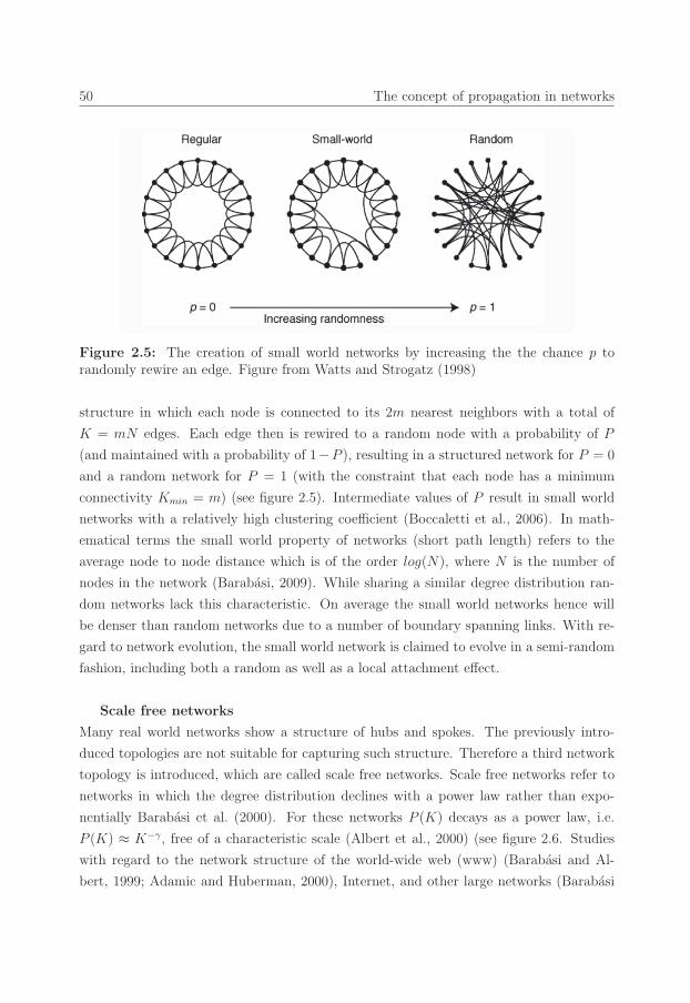
32_Erim_Vermeer Stand.job
50 The concept of propagation in networks
Figure 2.5: The creation of small world networks by increasing the the chance p torandomly rewire an edge. Figure from Watts and Strogatz (1998)
structure in which each node is connected to its 2m nearest neighbors with a total of
K = mN edges. Each edge then is rewired to a random node with a probability of P
(and maintained with a probability of 1−P ), resulting in a structured network for P = 0
and a random network for P = 1 (with the constraint that each node has a minimum
connectivity Kmin = m) (see figure 2.5). Intermediate values of P result in small world
networks with a relatively high clustering coefficient (Boccaletti et al., 2006). In math-
ematical terms the small world property of networks (short path length) refers to the
average node to node distance which is of the order log(N), where N is the number of
nodes in the network (Barabasi, 2009). While sharing a similar degree distribution ran-
dom networks lack this characteristic. On average the small world networks hence will
be denser than random networks due to a number of boundary spanning links. With re-
gard to network evolution, the small world network is claimed to evolve in a semi-random
fashion, including both a random as well as a local attachment effect.
Scale free networks
Many real world networks show a structure of hubs and spokes. The previously intro-
duced topologies are not suitable for capturing such structure. Therefore a third network
topology is introduced, which are called scale free networks. Scale free networks refer to
networks in which the degree distribution declines with a power law rather than expo-
nentially Barabasi et al. (2000). For these networks P (K) decays as a power law, i.e.
P (K) ≈ K−γ , free of a characteristic scale (Albert et al., 2000) (see figure 2.6. Studies
with regard to the network structure of the world-wide web (www) (Barabasi and Al-
bert, 1999; Adamic and Huberman, 2000), Internet, and other large networks (Barabasi

33_Erim_Vermeer Stand.job
2.3 The network structure 51
et al., 2000, 2001) indicate that many real world systems belong to this class of networks.
This topology is further characterized by even shorter path lengths and higher clustering
coefficients. The evolutionary process of scale free networks is related to what has been
labeled as preferential attachment. This effect refers to the notion that actors entering the
network are more likely to connect to other actors which have high prestige, in network
terms this would be those which have a high centrality, explaining the hubs and spokes
structure.
Figure 2.6: The degree (number of connections) distribution of a scale-free network
2.3.2 Topologies and propagation
By comparing among network topologies it has been shown that random and regular
networks are poor at facilitating propagation, small-world networks by leveraging the
short average path length are much better at doing so (Pastor-Satorras and Vespignani,
2001b; Pandit and Amritkar, 2001). Even more so scale-free networks by leveraging the
presence of hubs (highly connected actors) yield the highest propagation effectiveness
(Pastor-Satorras and Vespignani, 2001a). It has also been shown that scale-free networks
are very robust at doing so (Albert et al., 2000). In the same body of work it has been
shown that clustering facilitates propagation within the cluster but not between the clus-
33_Erim_Vermeer Stand.job
52 The concept of propagation in networks
ters(Rahmandad and Sterman, 2008).
These results indicate the relevance of the underlying characteristics of these topologies in
facilitating propagation. Both the skewness of the degree distribution, the average path
length and the clustering coefficient seems to play a facilitating role for propagation. While
this does not yield a full overview of the effects of network structure, it certainly provides
proof of the impact the system level network structure can have on propagation dynamics.
2.3.3 The micro level perspective of network structure
An argument can be made that the system level perspective of the networks structure
ignores details of the network structure which can be critical in order to understand the
propagation dynamics. Therefore the second stream of propagation literature has adopted
a bottom-up approach and considers the effect of network structure to stem from local
heterogeneity in the network. Local network structure captures network properties from
the perspective of the actor. Note that this is not the same as looking at the ego network,
but it does take the ego as the starting point of describing the network structure and its
effects. The claim is that the characteristics of local network structure can be aggregated
to describe properties of the complete network and hence are a fair representation of the
network as a whole.
Dyads
A structure connecting two actors, the dyad, can be considered as the smallest level of
local network structures. While the propagation literature mention the dyad is relatively
limited, there are two fundamental propagating forces at play at this level; reciprocity
and tie strength.
Reciprocity which is of interest in especially social network studies (Larson, 1992; Nowak,
2006) measures the extend to which actors respond to one another within the dyad. It
suggests that once a flow of information has occurred in a one direction it is likely that at
a later stage a similar flow will occur in the opposite direction. Suggesting that history
within the dyad can stimulate propagation.
Tie strength (Granovetter, 1973) is a characteristic commonly studied at the dyadic level.
It is argued that stronger ties are more likely to yield flow of information (even though the
information might be less valuable). By aggregating these local measures one can gain
insight into the characteristics of the network as a whole, and consequently make claims

34_Erim_Vermeer Stand.job
2.3 The network structure 53
regarding the propagation potential of the network on the system level.
Arguably, information on dyads in isolation should not be considered to describe struc-
tural properties of a network, as it does not provide any insight in how connections are
related to each other.
Triads
By increasing the number of actors to be considered by one triadic structures can be
created. These triads do capture the interrelated nature of connections and therefore are
assumed to be the smallest unit of analysis for describing (local) network structure. As
triads actually incorporate network effects, is a commonly studied local network structure.
Triad can occur in potential forms (for argumentation sake we neglect the fact that ties
can be directed); one of closure (Coleman, 1988) or one with a structural hole (Burt,
2005). The difference between these structures lies in the (lack of) presence of the third
tie. In a brokerage situation actor A enables interaction between two other actors, B
and C, which are not directly connected. In a situation of closure all three actors are
connected to each other (Figure 2.7).
Figure 2.7: Brokerage versus Closure
Being in a brokerage position has two ben-
efits; First as a bride between to uncon-
nected actors, a broker has control over
the flows between these actors. Second, all
flows go via the broker it is able the recom-
bine such flows before any of the alters can,
resulting in an information benefit.
From the propagation perspective broker
are critical as they connect two otherwise
unconnected parts of the network. This in-
dicates that betweenness, the extend to which an actor is on the shortest path between
other actors in the systems, is a key factor in propagation.
In a situation of closure all three actors are connected to each other, which results in them
all having equal power. Actors who try to pressure their alters can be corrected for their
behavior, as the alters are able to form coalitions. This results in a situation in which
negative actions can be countered and hence will be less likely to occur. The benefits of
such a situation are claimed to be closer collaboration, more trust between the actors and
increased sharing (resulting in shared norms), indicating that closure situations are more

34_Erim_Vermeer Stand.job
54 The concept of propagation in networks
prone to propagation in the network.
Figure 2.8: Examples of networkmotifs - note that in these examplesthe connections are assumed to bedirected.
Motifs
Further increasing the size of the structure can be
done by adding one or more connections to the net-
work of an alter. Network structures which include
the connections of the alters beyond distance 1 are
called network motifs (Milo et al., 2002; Alon, 2007).
These network motifs hold critical information re-
garding the local structure.
Consider an example (Figure 2.8, top structure) in
which an actor A has a brokerage position over B
and C. The extent to which this actor A is able to
broker however strongly depends upon potential al-
ternatives B and C have to interact. The presence
of an actor D which is structurally equivalent to al-
ter A will significantly reduce the influence of broker
A.
Motifs can be used to characterize the network structure on the system level (Milo et al.,
2002), but has not been linked to propagation dynamics, even though there seems to be
an apparent connection between the two.
2.3.4 The impact of network structure on propagation
While the range of local structures is virtually limitless, most of them describe a sub-set
of actors. This sub-set is bigger than that considered on the mirco-level, but smaller
than the system as a whole. These sub-sets of actors constitute the meso-level structural
measures. Most comonly these meso level measures revolve around clustering and com-
munities in the network (Girvan and Newman, 2002), or different types of centrality such
as betweenness centrality (Freeman, 1977) and eigenvector centrality (Bonacich, 2007).
Many meso-level structural characteristic are (to some extend) interrelated, making it
difficult to consider them in isolation, especially in real world networks. In such networks
there is no way to control for interactions, therefore most studies on the impact of net-
work structure are done using synthetic networks. In these networks a specific structural
characteristic can be manipulated while keeping other characteristics as stable as pos-
sible. By doing so it has for example been shown that, a shorter average path length
35_Erim_Vermeer Stand.job
2.4 The seed of infection 55
and the presence of long jumps (links connecting otherwise distant part of the network)
(Pastor-Satorras and Vespignani, 2001b; Pandit and Amritkar, 2001), a scale-free degree
distribution (Pastor-Satorras and Vespignani, 2001a), and an increased density (Burt,
2005) increase the speed and impact of propagation. On the other hand it has been
shown that fully random or regular network are generally poor at facilitating propaga-
tion (Watts, 1999) and that clustering facilitates propagation within the cluster but not
between the clusters(Rahmandad and Sterman, 2008).
A critical note should however be placed at the generalizability of such findings. They
have been obtained assuming there is no impact of the mechanism of propagation. Con-
sequently all effects found have been attributed to network structure. It could however
be that the structure has different effect across different mechanisms of propagation.
2.4 The seed of infection
The third driver of propagation dynamics identified in literature is the seed of infection.
This seed refers to the initial location (actor, or group of actors) at which the propagation
phenomenon enters the system. While the seed is commonly mentioned and studied in
literature (e.g. (Stonedahl et al., 2010)) as a driver of propagation this seems to be an
incorrect assumption. Taking a pragmatic look at this driver indicates that the seed will
only impact the propagation dynamics when heterogeneity in the can be leveraged. In a
scenario in which the network is completely homogenous, the network will look exactly
the same regardless of where the propagation process will enter the network, consequently
the seed will cause no variation in the dynamics of the subsequent propagation process.
Therefore the impact attributed to the seed of infection in fact stems from the assumption
that networks are heterogeneous, suggesting that the heterogeneity in the system is the
real driver of propagation dynamics.
In scenarios where the system is heterogeneous, the structure of the network will differ
depending on which part of the network is considered. Depending on the choice of seed, a
different structure can be faced in the early stages of propagation. As this local structure
serves as the infrastructure underlying propagation in the earliest stages, it will restrict
the initial propagation dynamics which in turn strongly affects the momentum a propa-
gation process can gain. This indicates that in heterogeneous scenarios the seed certainly
does matter.
Essentially it is the local dynamics which drive the system-wide dynamics. This suggests
that things which can cause heterogeneity in the the local dynamics have the potential
to affect the propagation dynamics on the system-level. The (local) network structure

35_Erim_Vermeer Stand.job
56 The concept of propagation in networks
can cause local variation in the dynamics, but also the actor behavior is likely to have a
strong effect. As the mechanism of propagation is made up from the behavior of actors,
the behavior by definition has an effect of the propagation dynamics. It is commonly
accepted that actors are heterogeneous by nature, no two actors are exactly the same,
and therefore their behavior will differ. This heterogeneity in actor behavior therefore will
cause variations in how propagation occurs locally. Consequently, this behavior is likely
to yield an effect on the propagation dynamics as a whole.
While the effects of heterogeneity have been studied in literature (Goldenberg et al.,
2001; Rahmandad and Sterman, 2008; Young, 2009; Jackson and Lopez-Pintado, 2013),
the results of these studies seem to be inconsistent at least. On the one had it is found
that heterogeneity plays a role in determining the propagation effectiveness (Jackson and
Lopez-Pintado, 2013), while other studied argue that such effect is neglectable (Rahman-
dad and Sterman, 2008). This suggest that the effect of heterogeneity on propagation
dynamics are not completely understood in current propagation literature.
2.5 More complex propagation processes
In describing the drivers of propagation dynamics literature has adopted relatively sim-
ple propagation processes. In reality propagation processes might however be quite more
complex. Thus far it has been assumed that each of the drivers (the mechanism, network
structure and local heterogeneity) has an independent effect on propagation dynamics.
This makes studying propagation far more easy, but might not be the most realistic as-
sumption.
Independence among the drivers of propagation dictates that during the radiation of (a
set of) signal(s) each of these signals is independently sent. Any signal being radiated
will have no effect on the other radiated signals. It therefore does not matter how many
signals are being radiated. Similarly during the reception process it is assumed that pro-
cessing of signals is independent of the amount of signals received.
Centola and Macy (2007) however put forward a complicating argument; they suggest
that in scenarios where the behavior being propagated is either costly, risky, or con-
troversial the willingness to participate in this behavior and consequently a change in
behavior/state of actors (reception) requires independent affirmation or reinforcement
from multiple sources. What this effectively does is break the linear relationship between
the amount of signals processed and the behavior. The reception behavior is significantly
different when two signals are received as compared to a single signal. As multiple signals

36_Erim_Vermeer Stand.job
2.5 More complex propagation processes 57
can only be a result of multiple incoming ties, this implies that the network structure will
affect the mechanism of propagation. Therefore the assumption that drivers are indepen-
dent is abandoned. The authors refer to this type of propagation as ‘complex contagion’,
and show that the interaction between drivers can yield propagation dynamics which are
significantly different from traditional propagation processes.
While complex contagion is but a single way of relaxing the assumption of independence of
drivers of the propagation dynamics, many similar notions of more complex propagation
processes can be found in literature and practice. For example the notion of information
overload refers to the idea that actors are bounded in their capabilities to process infor-
mation (Simon, 1982). This bounded capacity will cause the efficiency by which actors
respond to signals (reception) to either be capped or at least show a concave relation-
ship with the incoming signals. Again as the amount of signals is dependent only on
the network structure, this suggests an interaction of the the network structure and the
mechanism of propagation.
Both the notions of complex contagion and bounded rationality refer to interaction among
signals during the reception sub-process. But a similar complicating mechanism can be
proposed for the radiation sub-process. An example is costly radiation. Costly radiation
assumes that the are costs involved with sending signals and that actors are limited in
the resources they have. Combined these constraints result in actors being restricted in
the extent to which they can or will send out signals.
Each of these examples captures some form of a more complex propagation behavior.
They all incorporate a notion of interaction among the drivers of propagation dynamics.
This adds another level of complexity to the propagation process, of which the effect have
not been structurally studied and hence remains poorly understood.
To explore this additional layer of complexity in a structured way, one needs to have
method in place which is able to distinguish between all three drivers of propagation. Only
when the the drivers can be identified the interactions among them can be considered.
And only when the interactions among them are considered one can start to understand
the complex propagation dynamics. While traditional models allow for incorporating the
effects of the seed (as well as local heterogeneity which drives this effect), and the network
structure, they generally lack a detailed description of the propagation mechanism. This
makes traditional propagation models ill-equipped to address this layer of complexity. In
contrast, the information processing view of propagation and the subsequent RTR-model
of propagation are designed to capture and describe the propagation mechanism, therefore
they are particularly well suited to study these more complex phenomena.

36_Erim_Vermeer Stand.job
37_Erim_Vermeer Stand.job
Chapter 3
The conceptual framework
In studying dynamics of propagation the literature chapter has introduced three drivers
of propagation; the network structure, the seed of infection and the propagation mecha-
nism. While there is literature describing the effects of network structure and the seeding
locations, literature on the mechanism of propagation is largely missing. We aim to fill
this gap in literature, and hence this dissertation will focus specifically on the mechanism
of propagation. It aims to shed light on the impact of the mechanism of propagation on
propagation dynamics, and by doing so increase the grip on these dynamics.
To describe the mechanism of propagation the information processing view of propaga-
tion, and the subsequent RTR-model of propagation, have been put forward. In this view
(and model) the propagation process is considered as an information processing process,
and consequently decomposed into three sub-processes; Radiation, Transmission and Re-
ception. These sub-processes describe how information is processed on the actor level,
and hence describe the mechanism of propagation.
In order to show the impact of the mechanism of propagation it is not sufficient to simply
link the mechanism to propagation dynamics. As there are multiple drivers of propaga-
tion, the interactions between all three drivers will determine the eventual propagation
dynamics. The impact of the mechanism should not be considered without also con-
sidering other drivers of propagation. Therefore, in this dissertation, the propagation
mechanism is linked not only to the dynamics of the propagation process, but also to
the two other drivers of propagation dynamics. Finally, the goal is to increase the grip
on propagation dynamics, an increased understanding of these dynamics would allow for
better intervention strategies, and it is argued to this research is a means to this end.
The resulting conceptual framework (depicted in figure 3.1) thus proposes four relation-
37_Erim_Vermeer Stand.job
60 The conceptual framework
ships. The first three relate to understanding the propagation dynamics, and are conse-
quently linked to three research questions. The latter focuses on the practical implications
of such an increased understanding.
The first relationship describes the direct effect of the mechanism of propagation on the
propagation dynamics. It can be linked to the first research question in this dissertation
which reads: ‘(How) do differences in the information processing at the actor level affect
system-wide propagation dynamics? ’.
The second relationship describes the interaction effect of the mechanism of propagation
and the network structure. It is assumed that the effects of network structure can be very
different under different mechanisms of propagation, suggesting that the mechanism has
a mediating effect on network structure. It can be linked to the second research question,
which reads: ‘How does information processing at the actor level affect the effects of net-
work structure on system-wide propagation dynamics? ’
The third relationship, implicitly considers the third driver of propagation, the seed of
infection. However, the seed of infection only has an impact on propagation dynamics
when there is heterogeneity in either the network structure or the behavior of actors in
the network. As heterogeneity in the network has already been covered in the second
relationship and question, the third relationship describe the effect of actor heterogeneity.
Rather than explicitly considering the seed of infection it thus focuses on that which makes
the seed a driver of dynamics, and considers the interaction between heterogeneity in the
actor behavior and the propagation mechanism. This relationship can be linked to the
third research question which reads: ‘What role does heterogeneity of actor information
processing behavior play on propagation dynamics? ’.
The fourth and last relationship, does not link to a specific research question, instead it
considers the practical value of the three questions posed before. Understanding the role
of the propagation mechanism on the dynamics is critical in terms of knowledge creation,
but the real value would be derived from that which can be done with such understanding.
When increased understanding results in better intervention strategies, it will allow for
increasing the grip on propagation dynamics.
To study the proposed relationships in the conceptual framework, each of the associated
research questions will be addressed in a separate study.
• Study 1 (chapter 4) will be aimed at considering the direct effect of the propagation
mechanism on propagation dynamics. It will describe the information processing
view of propagation and the model of propagation capturing this view, the RTR-
model of propagation. It captures the potential effects of difference in the propa-
gation mechanisms and will provide validation with of the new propagation model.
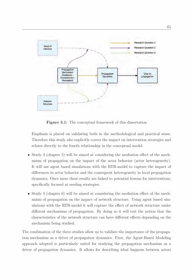
38_Erim_Vermeer Stand.job
61
Figure 3.1: The conceptual framework of this dissertation
Emphasis is placed on validating both in the methodological and practical sense.
Therefore this study also explicitly covers the impact on intervention strategies and
relates directly to the fourth relationship in the conceptual model.
• Study 2 (chapter 5) will be aimed at considering the mediation effect of the mech-
anism of propagation on the impact of the actor behavior (actor heterogeneity).
It will use agent based simulations with the RTR-model to capture the impact of
differences in actor behavior and the consequent heterogeneity in local propagation
dynamics. Once more these results are linked to potential lessons for interventions,
specifically focused at seeding strategies.
• Study 3 (chapter 6) will be aimed at considering the mediation effect of the mech-
anism of propagation on the impact of network structure. Using agent based sim-
ulations with the RTR-model it will capture the effect of network structure under
different mechanisms of propagation. By doing so it will test the notion that the
characteristics of the network structure can have different effects depending on the
mechanism being studied.
The combination of the three studies allow us to validate the importance of the propaga-
tion mechanism as a driver of propagation dynamics. First, the Agent-Based Modeling
approach adopted is particularly suited for studying the propagation mechanism as a
driver of propagation dynamics. It allows for describing what happens between actors

38_Erim_Vermeer Stand.job
62 The conceptual framework
during propagation, and thus facilitates characterization of the local propagation mech-
anism. By doing so it allows system-wide dynamics to ’emerge’ from local interactions
without making a priori assumptions on how the system-wide dynamics will occur, which
allows exploration of the effects on propagation dynamics.
Second, considering not only the direct effect of the mechanism but also the interaction
with the other drivers of propagation dynamics, places the research within a larger con-
text. While this might make settings very explicit, limiting the generalizability, it strongly
increases the accuracy of the models and their findings, making them more suitable for
being translated into practice.
Third, by considering also the practical relevance it not only considers whether the mech-
anism makes a difference, but also whether this is difference that makes a difference.

39_Erim_Vermeer Stand.job
Chapter 4
Study 1: The RTR-model of
propagation
Coauthors1: O.R. Koppius, P.H.M. Vervest
Abstract: The study of network dynamics often focuses on the process of propagation; the
process by which a change in the state of a focal actor results in a change of state in one
or more of its connected neighbors. Propagation is studied in various fields under labels
such as contagion, diffusion, spread, cascades or influence.
Many previous studies of propagation have assumed propagation to refer to the process
by which actors adopt a change in state. While this is an essential part of propagation,
we claim that adoption of a state-change is only part of the propagation process and that
propagation is actually a combination of three distinct sub-processes: Radiation, the send-
ing of a signal, Transmission, the transport of the signal, and Reception, the response to
a signal (RTR). We put forward a model for propagation based on these three distinct
sub-processes.
We show that the sub-processes can be used to sub-divide potential interventions in the
propagation process, in which each intervention can be mapped to a change in a particular
sub-process. Using simulation with the RTR-model we show that understanding the differ-
ent components of propagation is essential for assessing the effectiveness of interventions.
Incorrect specification can lead to an over- or underestimation of the effectiveness of an
intervention by almost an order of magnitude. This indicates that to manage the outcomes
1This chapter considers a working paper. Preliminary versions of this paper have been presented atWorkshop Information in Networks (WIN) in 2012 and 2013 and the conference for complexity in business(CCB) in 2013.

39_Erim_Vermeer Stand.job
64 Study 1: The RTR-model of propagation
of propagation and understand how to intervene effectively during propagation, it is vital
to understand the role of the three distinct aspects of the RTR-model.

40_Erim_Vermeer Stand.job
65
Propagation in networks refers to the process by which a change in the state or behav-
ior of an actor results in a change of state or behavior in one or more of its connected
neighbors. It covers processes such as spread of disease, diffusion of information or social
influence. In literature the propagation process has been studied in various fields and is
known under labels such as contagion (Centola and Macy, 2007; Dodds and Watts, 2004),
diffusion (Reagans and McEvily, 2003; Rogers, 1995; Valente, 2005), cascades (Buldyrev
et al., 2010; Buzna et al., 2006) or influence (Aral et al., 2009, 2013). In many of the
propagation studies the structure of interactions among the actors, the network struc-
ture, has been the focus of attention. Studies that look at the role of network topology
Dodds and Watts (2004); Albert et al. (2000); Pastor-Satorras and Vespignani (2001a),
clustering (Centola and Macy, 2007; Dodds and Watts, 2004) or local network structures
such as hubs (Boccaletti et al., 2006) or weak ties (Granovetter, 1973) have pointed out
the importance of the network structure in determining the outcomes of the propagation
process, suggesting it is the key to understanding the impact of interventions in the prop-
agation process. In these studies however the role of the mechanism of the propagation
process itself is often overlooked.
Previous work on propagation has adopted a variety of propagation dynamics (Bass, 1969;
Valente, 1996; Kempe et al., 2003) depending on the field in which it is studied. In epi-
demics we speak of an infection rate, in management or social studies of an adoption
threshold, and in physics of the percolation probability. While these dynamics assume
a different mechanism of propagation they do share one commonality; the process by
which the behavior or state of an actor (A) will result in a change of behavior or state of
connected neighbor (B) is considered by means of a single rate or likelihood, and hence
propagation is considered to be monolithic. Drawing on communication theory (Shan-
non, 1948), we however state that the mechanism of propagation is composed of three
distinct sub-processes, Radiation, Transmission and Reception (RTR) (Figure 4.1), each
with their own parameter (α, φ, η).
Radiation (α) refers to the process by which a change in the state or behavior of an actor
results in that actor sending out signals to its outgoing ties. Transmission (φ) refers to
the process by which a signal is transferred from the sender to the receiver (via a tie).
Reception (η) refers to the process by which actors respond to the incoming signal(s) and
change their behavior or state accordingly. Only when all three sub-processes have taken
place can we speak of propagation.
For example, propagation of disease requires an actor to spread the virus/germ (radia-

40_Erim_Vermeer Stand.job
66 Study 1: The RTR-model of propagation
Figure 4.1: Propagation is divided in three distinct sub-processes; Radiation refers tothe process with which an actor translates a change in state into an outgoing signal,Transmission to the process by which this signal is transferred (via a tie) towards thealter(s), and Reception to the process by which alters respond to the incoming signal andmay change state accordingly.
tion), the virus/germs to be transferred to the alter(s) (transmission), and the alter(s) to
get sick in response (reception). Similarly, the spread of a financial crisis requires banks
to become insolvent and default on loans (radiation), this will affect the liquidity of the
counterpart (transmission) but only result in propagation when the counter-part become
insolvent as well (reception).
While current propagation models, using a single parameter, allow for variations in the
rate of successful propagation, they make no distinction among the sub-processes in the
propagation mechanism. Hardly ever claims are being made about which part of the
mechanism is considered, and hence sub-processes are frequently used inter-changeably.
Commonly literature refer to a process which resembles infection or adoption (Table 4.1)
(mostly referred to as λ); they consider how actors respond to signals. In doing so how
the signal reaches the actor is often ignored, and thus focus in literature has mainly been
on the reception sub-process.
By not explicitly distinguishing the sub-processes of propagation and using them inter-
changeably, it is assumed that each of they has the same effect on propagation, and
that propagation mechanism thus can be considered as a homogeneous process. This
assumption of homogeneity does reduce the complexity of propagation, but also limits
the potential for describing the underlying mechanism of the process. Recent work (Cen-
tola and Macy, 2007; Aral et al., 2013; Banerjee et al., 2013) has found that neglecting
these mechanics can have unforeseen and far-reaching consequences, suggesting that more
attention needs to be paid to the mechanism underlying the propagation process. Cen-
tola and Macy (2007) in his study on complex contagion has shown that both the speed
and pervasiveness of propagation are strongly influenced by claiming that for an actor to

41_Erim_Vermeer Stand.job
67
Table 4.1: This table depicts the way in which propagation has been operationalized inrecent literature. Different streams of literature focus on different sub-processes, and thuscapture only part and not the whole propagation process.
Author Year Label ofpropagation
Sub-process considered
Radiation Transmission Reception
Granovetter 1973 Diffusion xRogers 1995 Diffusion xReagens and McEvily 2003 Diffusion xDodds and Watts 2004 Contagion xValente 2005 Diffusion x xBuzna et al. 2006 Cascades xCentola and Macy 2007 Contagion xRahmandad and Ster-man
2008 Diffusion x
Buldyrev et al. 2010 Cascades x xIyengar et al. 2011 Contagion xAral et al. 2013 Influence x xBanerjee et al. 2013 Contagion x x
41_Erim_Vermeer Stand.job
68 Study 1: The RTR-model of propagation
change state, multiple stimuli are needed. Furthermore, the notion that actors can send
out very different strengths of signals (Aral et al., 2013; Banerjee et al., 2013) and/or be
susceptible to different magnitudes of signals (Aral et al., 2013) have been shown to have
a strong influence on the outcomes of propagation. These results indicate that variations
in process mechanism have a marked effect on the outcomes of the propagation process,
suggesting a need to focus on the process itself rather than on the network structure.
The need to pay attention to the sub-processes of propagation becomes even more appar-
ent when one considers changes in the propagation process. Such changes can be either
unintentional or made in order to steer propagation, in which case we refer to them as in-
terventions. Closely looking at such interventions reveals that each intervention is in fact
aimed at changing a specific sub-process. The set of interventions described by Valente
Valente (2012) can each be linked to a specific single sub-process: selecting leaders who are
able to persuade others would be a radiation-based intervention; selecting low-threshold
agents who easily change they state or behavior would be a reception-based intervention;
and both induction and alteration which focus on the structure that facilitates transfer
would be transmission-based interventions. Similarly, the interventions made to steer the
outcomes of propagation processes in practice (Table 4.2), can be mapped to specific sin-
gle sub-processes.
The notion that interventions are linked to a single sub-process rather than to the propaga-
tion process as a whole changes our perspective on how interventions work. Rather than
changing the outcomes, the dynamics of the propagation process, interventions change
the very mechanism that underlies them. These changes in mechanism in turn result
in differences in the dynamics. Consequently, steering the outcomes of propagation now
becomes a question of knowing how precisely interventions change the mechanism of the
propagation process. Traditional single-parameter models adopt an oversimplified notion
of the propagation mechanism, they assume homogeneity among the sub-processes, which
makes them inadequate for dealing with variations in the mechanism and distinguishing
between the effects of different types of interventions. Studying the impact of interven-
tions therefore requires a new type of propagation model.

42_Erim_Vermeer Stand.job
4.1 The Radiation-Transmission-Reception model 69
4.1 The Radiation-Transmission-Reception model
We put forward a new model, the Radiation-Transmission-Reception model of propaga-
tion or RTR-model. This model describes the propagation mechanism on the dyadic level
(between two actors), and hence can be considered as an Agent-Based Model for propaga-
tion. In its general form, the RTR-model consists of functions for Radiation, Transmission
and Reception (full description in the supplementary information[SI]) which consequently
allows a change in state to propagate from one actor to its connected neighbors (alters).
The radiation function describes how the change in state of an actor i (Δsi,t), if higher
than the radiation threshold (u), will result in a signals being sent (pouti,e,t ∈ P outi,t ) to the
outgoing ties (Eouti ).
t∑t′=t−Trad+1
∑(Ai,t′ × P out
i,t′ × (τrad)(t−t′)+1) =
⎧⎨⎩Δsi,t if Δsi,t ≥ u
0 if Δsi,t < u(4.1)
In which Ai,t (αi,e,t ∈ Ai,t) is a vector of capturing the characteristics which influence the
radiation per outgoing edge, Trad is the radiation memory duration, the number of time
units after a change of state that this change can cause radiation, and τrad is the memory
inflation factor, the extend to which past changes are amplified or dampened.
The transmission function describes how the signal radiated (pouti,e,t ∈ P outi,t ) is transformed
into the signal which is received by the alter j (pine,j,t)
pouti,e,t =t∑
t′=t−Ttra+1
(φe,t′ × pine,j,t′ × (τtra)(t−t′)+1) (4.2)
In which Ttra is the memory duration for transmission, τtra is the memory inflation factor
for transmission, and φe,t is a vector of edge characteristics which influence transmission.
The reception function describes how transmitted signals (pine,i,t) received from the incom-
ing ties (Eini ) translate into a change of state of an alter if their combined effect passes
the reception threshold (q).
Δsi,t =
⎧⎪⎪⎪⎪⎪⎨⎪⎪⎪⎪⎪⎩
t∑t′=t−Trec+1
∑(P in
j,t′ ×Ψj,t′ × (τrec)(t−t′)+1) , if
t∑t′=t−Trec+1
∑(P in
j,t′ ×Ψj,t′ × (τrec)(t−t′)+1) ≥ q , otherwise
0
(4.3)

42_Erim_Vermeer Stand.job
70 Study 1: The RTR-model of propagation
Table 4.2: Examples of interventions in propagation in practical settings. For eachsetting it shows how the propagation process can be divided into three sub-processes andhow different interventions are linked to specific sub-processes.
Setting Radiation Transmission Reception
Process Intervention Process Intervention Process Intervention
Spread of
financialcrisis
A bank be-comes insolventand defaults ona loan
Capital in-jections fromcentral banksmay changethe state ofthe insolventbank, makingit solvent againbefore anypropagationcan occur. Thisprevents theradiation of asignal.
The loans be-tween bankscauses thedefault of onebank to resultin a loss fora connectedbank.
Guarantees,securities andderivativescan ensuredefaulted loansare still (par-tially) covered,reducing thesignal whichreaches thealter.
The other bankwill incur aloss from thedefaulted loanand can absorbthis loss orchange stateto becomeinsolvent.
Enforcing anincrease in theliquidity buffersresults in banksbeing less likelyto also becomeinsolvent whenincurring lossesfrom otherdefaults.
Contagionof disease
A person be-comes sick andspreads the vi-ral load/germsin the directionof others, i.e.through sneez-ing.
Quarantineinterventions,such as tellingpeople tostay at home,reduce their in-teraction withfriends andhence reducethe chance ofspreading thedisease to thesefriends.
The trans-fer of viralload/germs toother people(alters), i.e.being hit bya sneeze ortouching acontaminatedsurface.
Getting thosepeople whoare infectedto wear pro-tective masks,and/or washtheir handsextensively willreduce the viralload/germs anindividual willspread andhence reducethe transmis-sion of thevirus to otherpeople.
The alters re-spond to the vi-ral load/germsbeing received.They attemptto fight off theinfection, andeither succeeds,so the diseasedoes not prop-agate, or failand gets sick.
Immunizationdecreases thesusceptibilityof actors, asimmunizedactors are con-sidered to reactdifferently toincoming sig-nals. Throughimmunization,the receptionprocess ofthese actors ischanged.
Adoptionof inno-vation
A firm adopts anew productiontechnique andits employeesstart to talkabout thisadoption.
Communicationor visibility isreduced orincreased bymeans of con-fidentiality oradvertisingagreements.
Other firms be-coming awareof the adop-tion, throughinteraction.This can be bycommunicationor observation.
By using a dif-ferent means ofcommunicationor changing thetransparencythe extentto which thesignal reachesan alter can bechanged.
Other firmsmake a decisionon whetherto also adoptthe innovation,based on thesignals theyreceive viatheir network.
By changingthe investmentcosts (sub-sidizing orlicensing) theother firms willbecome more,or less, proneto adopt theinnovation.
Diffusionof infor-mationor knowl-edge
A person hasa certain pieceof novel infor-mation and de-cides to sharethis.
Rewardingsharing activitywith status (asis often done ononline forums)incentivizesthe sharing ofinformation.
Communicationamong individ-uals allows theinformation tobe spread fromone person toanother.
By using a dif-ferent medium(e.g., telegramvs. videocon-ferencing) therichness ofcommunicationcan be changed,thus improvingor reducing theextent to whichthe informationis understoodduring trans-mission.
The alterreceives theinformationand fits this tohis or her exist-ing knowledgeand decides toaccept or rejectthe informa-tion, in full orin part.
By decreasingor increasingthe utility (nov-elty) of theinformationbeing shared,the willingnessto accept suchinformation canbe increased.
43_Erim_Vermeer Stand.job
4.2 Methods and Data 71
In which Trec is the memory duration for reception, τrec is the memory inflation factor for
reception, and Ψi,t (ηe,i,t ∈ Ψi,t) is a vector capturing actor specific characteristics influ-
encing the reception per incoming edge. Using equations 4.1, 4.2 and 4.3, the RTR-model
decomposes the single-parameter propagation process into three distinct sub-processes.
What becomes clear when considering these sub-processes is that the each of them adopts
a different logic. Radiation is a process from one actor to its outgoing ties, making it
essentially a one-to-many process. Transmission occurs within a single tie and hence is
one-on-one process. Reception is a process from many incoming ties to one single actor,
making it a many-to-one process. Only by knowing what is actually happening during
each step of propagation and describing the propagation process in terms of three distinct
sub-processes one can understand the impact of interventions on the overall propagation
likelihood and get a grip on the propagation dynamics.
4.2 Methods and Data
To indicate the relevance of using the RTR-model and the subsequent decomposition of
propagation into three distinct sub-processes we will adopt a two-staged approach; first,
we show that using this model allows for a better representation of propagation field data,
and second, by means of simulation, we will show that knowing the three sub-processes
is critical in order to effectively intervene in the propagation process.
While the sub-processes are conceptually different, data on propagation processes often
only measures the outcomes of propagation (actors adopt or not), and hence lacks this
distinction. Consequently, measurements of separate sub-processes are rare. As measuring
the individual sub-processes is difficult, modeling the division into sub-processes will only
yield relevant insights if these sub-processes can in fact be deduced from the observed
outcomes in field data. Therefore in the first part of the analysis we justify dividing
propagation into sub-processes by applying the RTR-model to field data relating to the
adoption of a software application called Yahoo! Go. We show that applying the RTR-
model not only enables us to parametrize the distinct sub-processes but also to generate
a model that is a better fit with the actual propagation data.
In the second part of the analysis we focus on the implications of using the RTR-model.
We show that only by dividing the propagation process into three sub-processes one can
understand why interventions vary in effectiveness.

43_Erim_Vermeer Stand.job
72 Study 1: The RTR-model of propagation
4.2.1 Field data
4.2.1.1 Yahoo! go 2.0 application adoption
In this section we apply the RTR-model to a real-world propagation setting: the adoption
of a mobile software application. We use data that describes the adoption of the Yahoo!
Go 2.0 application among approximately 27 million users of Yahoo messenger (Yahoo!,
2010) as collected by Aral et al. (2009). Drawing on instant messages among users we
create a weighted network over which adoption can spread (more details on the data can
be found in SI and Aral et al. (2009)) and track the spread over a period of four weeks.
We assume this propagation to be based on the buzz created by adoption, suggesting that
after adoption users will start sending out (radiate) signals towards other people, but will
only do so for a limited period of time (in our case, one week). This has two implications
for the way in which we study propagation in this setting. First, there is only a limited
number of states that actors can be in; they are either able to adopt (susceptible) or
have adopted already (infected). As we consider a propagation process driven by buzz,
adopters will stop sending out signals and are permanently in an infected state (they are
removed) a week after being infected, effectively making this model an SIR (Susceptible,
Infected, Removed) model. Second, because actors send out (radiate) signals only while
they are in the infected state, we consider only the interactions during this period as being
important for propagation (we do not consider any previous interactions).
4.2.1.2 Applied Radiation-Transmission-Reception model
In our empirical setting we are considering a scenario in which actors can only have
limited amount of states (they are susceptible, infected or removed) like the SIR models
which traditionally used to model contagion of disease. Therefore, we restructure the
general RTR-model, which is deterministic in nature, into a stochastic variant which
resembles SIR model logic (for a detailed description see [SI]). This stochastic variant can
be summarized as follows:
• Each actor in the system has a state (si,t): either Susceptible, Infected or Removed.
• Each infected actor in any time-step has a probability (αi,t) of sending out a signal
to and activating an outgoing tie for transmitting a signal (all ties are considered
separately).
• Each activated tie has a probability (φe,t) of transmitting the signal which has been
radiated at the same time-step.
44_Erim_Vermeer Stand.job
4.2 Methods and Data 73
• Each actor in the system has a probability (ηi,t) of changing to an infected state due
to any single incoming signal (we assume no interaction among signals, therefore all
signals are considered sequentially).
Our formulation dictates that the extent or likelihood of propagation (λ) is a product of
the three sub-processes (λ = αφη). Using a brute-force simulation approach (see [SI]),
we retrieve the system-wide parameters (radiation, transmission and reception) for the
stochastic RTR-model. We do so by simulating RTR-models with different parameters and
picking the parameters which most accurately reproduce the real propagation found in the
Yahoo! Go adoption data. We compare these results with those obtained from traditional
single-parameter propagation models. We have chosen four single-parameter models; the
first model, based on current literature, assumes no differences and interchangeability
among sub-processes. All sub-processes play an equal part in the propagation process
and hence always have the same value (α = φ = η). The latter three single parameter
processes are traditional propagation processes mapped onto the different sub-processes,
effectively assuming that it is a single sub-process —Radiation, Transmission or Reception
respectively— which drives propagation (and that the other two sub-processes will always
occur and thus do not play any role).
4.2.1.3 Results
Our results (Table 4.4 and Table 4.5) indicate two things: That we can distinguish the
separate sub-processes and that by dividing the propagation process into sub-processes
we have constructed a better fitting model of propagation ( at least in this setting).
First and foremost, the optimal parametrization found using our brute force method (Ta-
ble 4.4) shows variations between the sub-process parameters. This implies that there are
differences between the three sub-processes in practice, contradicting the assumption of
homogeneity and hence justifying the use of the RTR-model, and using three sub-processes
to model propagation. Even more so it indicates that without gathering additional data
we can re-analyze existing propagation processes to obtain the parameters for the spe-
cific sub-processes. We find that the optimal parametrization of sub-processes strongly
depends on the fit measure applied, raising the question whether there is in fact a single
stable parametrization for a propagation process. While this question is outside the scope
of this research, it certainly poses an interesting direction for future research.
Second, the fitting results (Table 4.5) reveal that the RTR-model has a lower level of error
and hence fits better than any single-parameter model, a result which has been found to
be robust over all fit measures used. To further examine the robustness of our results (see
44_Erim_Vermeer Stand.job
74 Study 1: The RTR-model of propagation
the [SI] for description robustness checks) also the Akaike information criterion (AIC) for
model performance (Akaike, 1974) has been included. This measure penalizes the use of
multiple parameters. Our results (Table 4.5) show that the RTR-model has the lowest
AIC scores of all tested models (52.68 compared to respectively 54.26, 53.80, 98.86 and
53.67), indicating that even when penalized for using more parameters the RTR-model
consistently outperforms the single parameter models in terms of reproducing real world
propagation data.
4.2.2 Impact of interventions
In the previous section we have shown the methodological validity of the RTR-model,
but in this section we will show the practical value of adopting the RTR-model. By
means of simulation we show that the impact of interventions depends strongly on the
decomposition of the propagation process. Hence effectively managing these processes
requires a detailed view of the propagation mechanism.
4.2.2.1 Simulation using the Radiation-Transmission-Reception model
In our simulation we again use a model in which the state of active actors is limited to
being either infected or susceptible, allowing the use of the probabilistic variant of RTR-
model (λ = αφη), similar to the one used while analyzing the field data. The simulation
model differs from the empirical setting in three ways: First, we consider actors to re-
cover rather than be removed, effectively making this a SIS model. We assume actors
to recover with a given likelihood (ρ), rather than being recovered automatically after
one time-step. Second, given that actors can be in the infected state for a longer period
of time, we consider them to radiate during each time unit in which they are infected.
Third, the network structure remains stable over the course of the simulation.
The simulation approach can be summarized as follows (a detailed description of the sim-
ulation method can be found in the IS). We run a set of 10,000 simulations on a given
stable network structure (undirected and scale-free, with 10,000 actors generated using the
Barabsi-Albert Barabasi and Albert (1999) approach), and for each of these simulations
we vary the seed of infection, effectively bootstrapping each scenario we simulate 10,000
times. We repeat this simulation process for multiple scenarios with the same overarching
propagation probability (λ) but different decomposition into three sub-processes. In line
with previous studies Albert et al. (2000); Pastor-Satorras and Vespignani (2001a, 2002)
we consider the proportion of infected actors in the system —the so-called pervasiveness—
to be the primary outcome variable.

45_Erim_Vermeer Stand.job
4.2 Methods and Data 75
We take a mean-field approach when considering the simulation results, averaging the
pervasiveness found over the bootstrapped set of simulation runs. Averaging these re-
sults over all potential seeds implies we lose the individual dynamics stemming from the
initial seed; this enables us to capture the effects of the variation in process dynamics
without having to worry about effects of the network structure. This approach does hide
many of the differences between the various scenarios studied, but even when using this
(over)simplified method and studying propagation outcomes at the mean-field level the
impact of studying the sub-processes of propagation becomes apparent when interventions
in the propagation process are considered.
We measure the effects of interventions by simulating a propagation process and inter-
vening in this process halfway through the simulation (at t = 50). As has been shown,
an intervention can be linked to a single sub-process, and consequently an intervention
is operationalized as a change in one of the sub-process parameters. As we consider the
sub-process parameters in a stochastic model —meaning they should be interpreted as
probabilities of success in each step in the propagation process—, any absolute change
made to a sub-process parameter translates into a change in the probability success for
that specific sub-process. While an intervention of any size could have been applied in
our simulations, we chose to use an intervention that would reduce the success chance
of a sub-process by 20%, effectively reducing either α, φ or η by 0.2. Generally we as-
sume that an intervention decreases (or increases) the likelihood that a sub-process will
successfully take place, and therefore an absolute parameter change is the most suitable
form of modeling interventions.
4.2.2.2 Results
Our simulation results (Figure 4.2, Figure 4.3, Figure 4.4) show that the same intervention
can have very different effects depending on the decomposition of the propagation process,
which is not surprising when we consider that λ = αφη. This formulation dictates that the
effect of an absolute change in either of the sub-processes on the propagation probability
(the effect on λ) will depend on the parameters of the other sub-processes. Therefore
the effect of an interventions can differ drastically, depending on the decomposition in to
sub-processes.
When considering the effects of adopting the RTR-model in this setting it is interesting to
compare the scenarios with heterogeneous sub-processes (scenarios 1-3: Figure 4.5, Figure
4.6, Figure 4.7) to the ones in which the sub-processes are assumed to be homogeneous
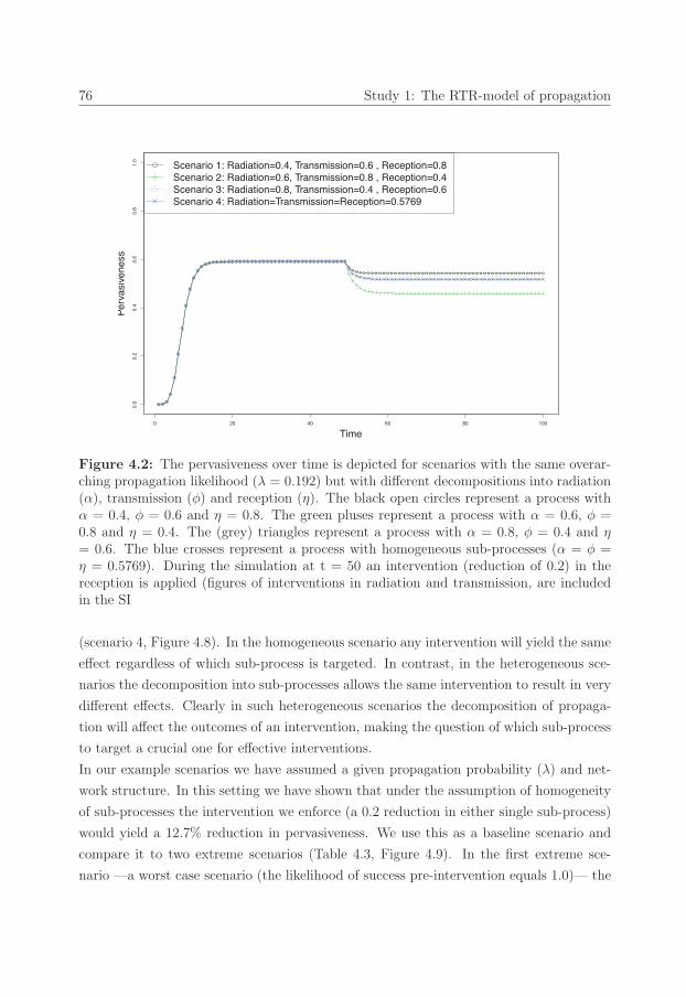
45_Erim_Vermeer Stand.job
76 Study 1: The RTR-model of propagation
0 20 40 60 80 100
0.0
0.2
0.4
0.6
0.8
1.0
Time
Per
vasi
vene
ss
● ●●
●
●
●
●
●
●
●
●
●● ● ● ● ● ● ● ● ● ● ● ● ● ● ● ● ● ● ● ● ● ● ● ● ● ● ● ● ● ● ● ● ● ● ● ● ●
●● ● ● ● ● ● ● ● ● ● ● ● ● ● ● ● ● ● ● ● ● ● ● ● ● ● ● ● ● ● ● ● ● ● ● ● ● ● ● ● ● ● ● ● ● ● ● ● ● ●
● Scenario 1: Radiation=0.4, Transmission=0.6 , Reception=0.8 Scenario 2: Radiation=0.6, Transmission=0.8 , Reception=0.4 Scenario 3: Radiation=0.8, Transmission=0.4 , Reception=0.6 Scenario 4: Radiation=Transmission=Reception=0.5769
Figure 4.2: The pervasiveness over time is depicted for scenarios with the same overar-ching propagation likelihood (λ = 0.192) but with different decompositions into radiation(α), transmission (φ) and reception (η). The black open circles represent a process withα = 0.4, φ = 0.6 and η = 0.8. The green pluses represent a process with α = 0.6, φ =0.8 and η = 0.4. The (grey) triangles represent a process with α = 0.8, φ = 0.4 and η= 0.6. The blue crosses represent a process with homogeneous sub-processes (α = φ =η = 0.5769). During the simulation at t = 50 an intervention (reduction of 0.2) in thereception is applied (figures of interventions in radiation and transmission, are includedin the SI
(scenario 4, Figure 4.8). In the homogeneous scenario any intervention will yield the same
effect regardless of which sub-process is targeted. In contrast, in the heterogeneous sce-
narios the decomposition into sub-processes allows the same intervention to result in very
different effects. Clearly in such heterogeneous scenarios the decomposition of propaga-
tion will affect the outcomes of an intervention, making the question of which sub-process
to target a crucial one for effective interventions.
In our example scenarios we have assumed a given propagation probability (λ) and net-
work structure. In this setting we have shown that under the assumption of homogeneity
of sub-processes the intervention we enforce (a 0.2 reduction in either single sub-process)
would yield a 12.7% reduction in pervasiveness. We use this as a baseline scenario and
compare it to two extreme scenarios (Table 4.3, Figure 4.9). In the first extreme sce-
nario —a worst case scenario (the likelihood of success pre-intervention equals 1.0)— the

46_Erim_Vermeer Stand.job
4.3 Conclusion 77
same intervention has an effect of reducing the pervasiveness by 6.1%, indicating the
lower bound of the intervention effect. In the second extreme scenario —a best case
scenario (likelihood of success pre-intervention equals 0.2)— the same intervention yields
a 100% reduction in pervasiveness (and hence eradicated the infection), indicating the
upper bound of the intervention effect. The differences in lower and upper bounds show
that assuming homogeneity among sub-processes (not decomposing propagation into sub-
processes), can lead to an overestimation of the effect of an intervention by a factor of 2
or an underestimation by a factor of 8. Even more so these bounds indicate that incorrect
decomposition in sub-processes can even yield an over- or underestimation by a factor of
14.
While these factors will clearly vary across scenarios being studied, variance of an order
of magnitude does pose a problem. It indicates that different mechanisms (decomposi-
tion into three sub-processes) can yield different intervention effects, suggesting that in
order to effectively intervene in the propagation dynamics one needs to know how the
propagation process is decomposed into sub-processes.
4.3 Conclusion
In this paper we put forward the notion that the propagation process is not monolithic and
that the mechanism by which it occurs should be decomposed into three sub-processes:
Radiation, Transmission and Reception. We propose a model incorporating these three
sub-processes (the RTR-model of propagation) which allows the capturing of differences
in the propagation process dynamics. We show that each of the sub-processes covers a
distinct part of propagation, therefore dividing the mechanism into sub-processes gives
us the ability to describe the process in more detail, and model behavior which can not
be modeled by using a single-parameter model. We corroborate this by showing that
the RTR-model is better able to reproduce real propagation phenomena than any single-
parameter model.
In our paper we also show that interventions are linked to specific single sub-processes,
therefore in order to evaluate the effectiveness of these interventions the sub-processes need
to be identified. We show that failing to correctly represent the sub-processes can yield
an under- or overestimation of intervention effects by more than an order of magnitude.
Our findings have important implications for decision-makers trying to steer propagation
processes. The use of the RTR-model provides a detailed description of the propagation
mechanism and effectiveness of interventions. As interventions in different sub-processes
require a different set of actions, this allows decision-makers to make more focused efforts

46_Erim_Vermeer Stand.job
78 Study 1: The RTR-model of propagation
Table 4.3: This table compares three scenarios with equal overarching propagationprobability (λ), a homogeneous scenario where each sub-process is equally strong, andthe two most extreme scenarios, a worst case scenario which is extremely resilient, and abest case scenario which is extremely volatile. It considers the effects of the same type ofintervention in each of these scenarios.
Scenario Pre-interventionpervasive-ness
Post-interventionpervasive-ness
Interventioneffect
Comparisonwith homoge-neous scenario
AbsoluteError
RelativeError
Homogeneous sub-processes:α = φ = η = 0.5796 0.592 0.517 12.7 %
Most resilient Sce-nario:likelihood of suc-cess pre-interventionequals 1
0.593 0.557 6.1 % -0.041 -52.0%
Least resilient Sce-nario:likelihood of suc-cess pre-interventionequals 1
0.592 0.000 100 % 0.517 687.4 %
at intervention and hence to become more effective in steering the propagation process
outcomes.
Our results suggest some interesting directions for future research. First, as previous
literature has often been unclear on which sub-process has been considered, it would
be valuable to reanalyze data sets used in existing literature to get an overview of the
impact of each sub-process on process outcomes. Second, while we have explored the
impact of differences in the propagation mechanism, we currently assume that all actors
behave similar. In many real-life situations we find that actors in fact differ in terms of
their contagiousness, transmission medium, and susceptibility, making this an interesting
extension to our model. Third, we have assumed a stable network structure, ignoring
the probable interaction between the structure of the network and process mechanism.
Studying this interaction would be a valuable avenue for future research.

47_Erim_Vermeer Stand.job
4.4 acknowledgments 79
4.4 acknowledgments
We would like to acknowledge Yahoo! Labs (http://webscope.sandbox.yahoo.com) for
providing access to the G7 - Yahoo! Property and Instant Messenger Data use for a
Sample of Users, v.1.0 database used in this study.
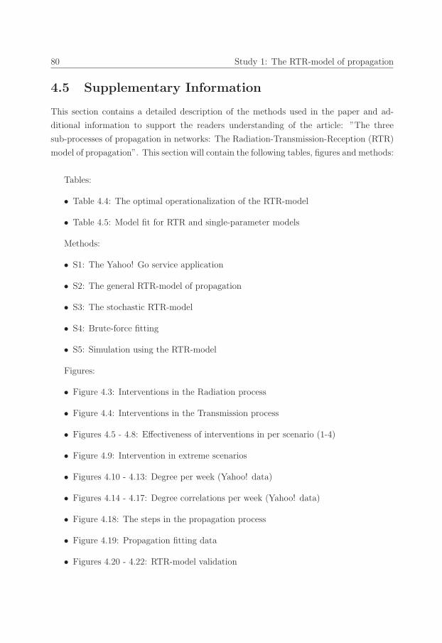
47_Erim_Vermeer Stand.job
80 Study 1: The RTR-model of propagation
4.5 Supplementary Information
This section contains a detailed description of the methods used in the paper and ad-
ditional information to support the readers understanding of the article: ”The three
sub-processes of propagation in networks: The Radiation-Transmission-Reception (RTR)
model of propagation”. This section will contain the following tables, figures and methods:
Tables:
• Table 4.4: The optimal operationalization of the RTR-model
• Table 4.5: Model fit for RTR and single-parameter models
Methods:
• S1: The Yahoo! Go service application
• S2: The general RTR-model of propagation
• S3: The stochastic RTR-model
• S4: Brute-force fitting
• S5: Simulation using the RTR-model
Figures:
• Figure 4.3: Interventions in the Radiation process
• Figure 4.4: Interventions in the Transmission process
• Figures 4.5 - 4.8: Effectiveness of interventions in per scenario (1-4)
• Figure 4.9: Intervention in extreme scenarios
• Figures 4.10 - 4.13: Degree per week (Yahoo! data)
• Figures 4.14 - 4.17: Degree correlations per week (Yahoo! data)
• Figure 4.18: The steps in the propagation process
• Figure 4.19: Propagation fitting data
• Figures 4.20 - 4.22: RTR-model validation

48_Erim_Vermeer Stand.job
4.5 Supplementary Information 81
Table 4.4: This table shows the parametrization of the RTR-model (into the three sub-processes) which best fit the actual propagation numbers found in the Yahoo! Go fielddata. A different fit measure has been applied for each model, reporting the total errorof the model for that measure.
Optimal parametrization of RTRRadiation Transmission Reception RMSE LRMSE RRMSE
0.1 0.3 0.1 684.20.1 0.1 0.2 0.9820.2 0.2 0.1 0.855
Table 4.5: This table shows the errors (and errors relative to the RTR-model) obtainedfrom the models which best fit the actual propagation numbers found in the Yahoo! Gofield data. The results of the three fit measures are shown for the RTR-model (which hasbeen fitted using single-decimal parameters), and four single-parameter models. The firstsingle-parameter model assumes all sub-processes are homogeneous and have the sameeffect and parameter ( α = φ = η) (and has been fitted using single-decimal parameters),the second single-parameter model is driven by radiation and assumes the other sub-processes always occur (φ = η = 1.0) (and has been fitted using two-decimal parameters),the third single-parameter model is driven by transmission and assumes the other sub-processes always occur ( α = η = 1.0) (and has been fitted using two-decimal parameters)and the last single-parameter model is driven by reception and assumes the other sub-processes always occur ( α = φ = 1.0) (and has been fitted using two-decimal parameters).
RTR-model Single-parameter modelsHomogeneous Driven by Driven by Driven by
Fit measure sub-processes Radiation Transmission Reception
RMSE 684.2 1374.0 1297.0 362381.2 1276.0(relative error) (200.8%) (189.6%) (52964.2%) (186.5%)
LRMSE 0.982 3.986 2.113 10.659 1.929(relative error) (405.9%) (215.2%) (1085.4%) (196.4%)
RRMSE 0.855 1.680 1.300 1.966 1.321(relative error) (196.5%) (152.0%) (229.9%) (154.5%)
AIC 52.68 54.26 53.80 98.86 53.67
48_Erim_Vermeer Stand.job
82 Study 1: The RTR-model of propagation
S1: The Yahoo! Go service application
In the first section of this paper, we analyzed the feasibility of using three sub-processes
to model propagation. In order to do so we need to be able to distinguish the three
sub-processes not only conceptually but also in practice. Therefore in this part of the
paper we consider a real-life propagation phenomenon: the adoption of the Yahoo! Go
2.0 application Yahoo! (2010). Yahoo! Go can best be described by quoting the authors
who initially collected this data (Aral et al., 2009): “The Yahoo! Go is a mobile soft-
ware application designed to deliver personalized content to users devices and to enhance
mobile search capabilities. Yahoo! Go provides personalized information across several
domains, including news, sports, weather, and financial information, as well as access
to e-mail, calendaring, location based services, photo sharing, and web search services.”
The Yahoo! Go dataset includes detailed demographic and daily usage behavior data
for approximately 27 million users, including geographic location and demographic data,
instant messaging (IM) usage behavior, PC usage behavior, mobile usage behavior, Go
usage behavior, and product adoption date for October 2007. A detailed description of
the data of this dataset can be found in the supplementary information of the work of
Aral et al. (2009). Only a sub-set of this information is used in our study; in order to
capture the propagation process in this data set we solely use the daily number of instant
messages among Yahoo! users (aggregated weekly) to construct a network of interactions,
and the adoption of the Yahoo! Go 2.0 application as the ‘behavior’ which spreads across
this network.
In our study a distinction is made between adoption and propagation. Whereas adoption
can refer to starting to use the Yahoo! Go application —which can be driven by any
form of external stimulus— we consider adoption as propagation only where it is poten-
tially driven by direct influence from someone else in the actor’s immediate neighborhood.
Therefore propagation relates to only those changes of state (adoptions) which occur when
an alter of the adopter has the infected state.
Descriptive Information for the Yahoo! Go dataset
The Yahoo! Go 2.0 dataset consists of a total of approximately 27 million unique users:
the descriptives of this dataset can be found in Table 4.6. As we are considering both the
behavior of users and the structure of the user community over a longer period of time, a
check for structural changes during that observation period is required. The descriptive
analysis of the data shows that not all actors are active during each of the time frames
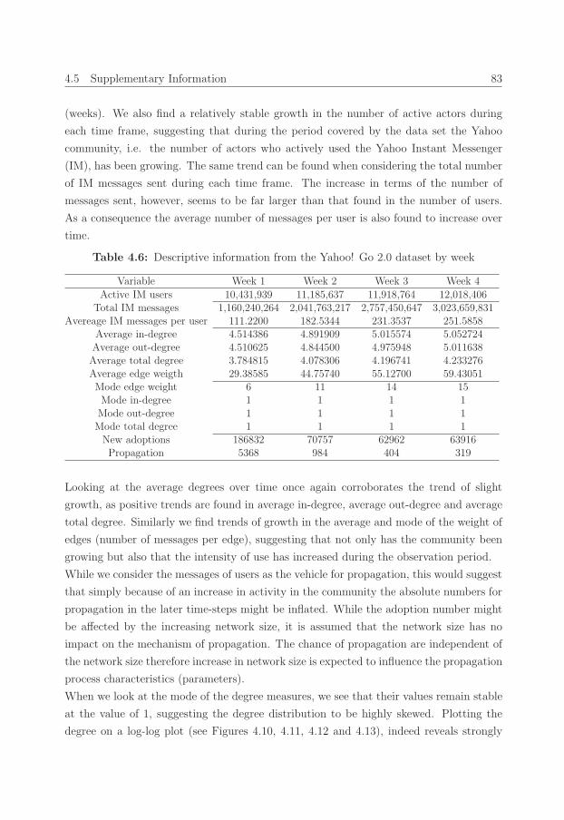
49_Erim_Vermeer Stand.job
4.5 Supplementary Information 83
(weeks). We also find a relatively stable growth in the number of active actors during
each time frame, suggesting that during the period covered by the data set the Yahoo
community, i.e. the number of actors who actively used the Yahoo Instant Messenger
(IM), has been growing. The same trend can be found when considering the total number
of IM messages sent during each time frame. The increase in terms of the number of
messages sent, however, seems to be far larger than that found in the number of users.
As a consequence the average number of messages per user is also found to increase over
time.
Table 4.6: Descriptive information from the Yahoo! Go 2.0 dataset by week
Variable Week 1 Week 2 Week 3 Week 4
Active IM users 10,431,939 11,185,637 11,918,764 12,018,406Total IM messages 1,160,240,264 2,041,763,217 2,757,450,647 3,023,659,831
Avereage IM messages per user 111.2200 182.5344 231.3537 251.5858Average in-degree 4.514386 4.891909 5.015574 5.052724Average out-degree 4.510625 4.844500 4.975948 5.011638Average total degree 3.784815 4.078306 4.196741 4.233276Average edge weigth 29.38585 44.75740 55.12700 59.43051Mode edge weight 6 11 14 15Mode in-degree 1 1 1 1Mode out-degree 1 1 1 1Mode total degree 1 1 1 1New adoptions 186832 70757 62962 63916Propagation 5368 984 404 319
Looking at the average degrees over time once again corroborates the trend of slight
growth, as positive trends are found in average in-degree, average out-degree and average
total degree. Similarly we find trends of growth in the average and mode of the weight of
edges (number of messages per edge), suggesting that not only has the community been
growing but also that the intensity of use has increased during the observation period.
While we consider the messages of users as the vehicle for propagation, this would suggest
that simply because of an increase in activity in the community the absolute numbers for
propagation in the later time-steps might be inflated. While the adoption number might
be affected by the increasing network size, it is assumed that the network size has no
impact on the mechanism of propagation. The chance of propagation are independent of
the network size therefore increase in network size is expected to influence the propagation
process characteristics (parameters).
When we look at the mode of the degree measures, we see that their values remain stable
at the value of 1, suggesting the degree distribution to be highly skewed. Plotting the
degree on a log-log plot (see Figures 4.10, 4.11, 4.12 and 4.13), indeed reveals strongly
49_Erim_Vermeer Stand.job
84 Study 1: The RTR-model of propagation
skewed distributions in each period. These distributions seem to follow a power-law, sug-
gesting that the IM network has in fact a scale-free structure. Scale-free networks are
often associated with large hubs. These hubs play a crucial role in the propagation pro-
cess as they are more likely to be connected to infected actors (high in-degree), making
them prone to be infected, and have many alters (high out-degree), allowing them to
cause widespread propagation once infected.
In the Yahoo IM network, however, there seem to be no such hubs. When one examines
the correlation between in- and out-degree (Figures 4.14, 4.15, 4.16 and 4.17 show the log-
log plot of the degree correlations) it reveals that the upper-right quadrant is completely
empty, indicating that there are no actors with both extremely high in- and out-degree.
Hence there are no actors who seem to fit the previously described hub role, a characteristic
which might hamper rapid propagation in this network.
S2: The general RTR-model of propagation
We put forward a generic model for studying propagation incorporating three sub-process;
Radiation, Transmission and Reception. Based on these sub-processes we formulate a
model of propagation consisting of three distinct functions; one for each of the sub-
processes. Hence the generic RTR-model of propagation consists of:
1. a Radiation function
2. a Transmission function
3. a Reception function
The propagation process has been defined as the process by which the change in state
of one (or more) vertices causes the change in the state of one (or more) of its alters.
The general RTR-model allows for modeling the propagation mechanism in a simple but
straightforward way. In this model we assume that there exists an underlying network
structure on which the propagation process will take place. This network structure can
be considered as a graph G = (V,E) with vertices i ∈ V := {1, . . . , n} and an edgeset
e ∈ E := {1, . . . ,m}. All edges are assumed to be directed and weighted, where wij,t
denotes the weight of the edge from vertex i to vertex jon time t, and [Wt] is the matrix
containing all edge weights on time t. All vertices i at any point in time have a state si,t,
and [St] is the matrix containing the state all actors at time t (si,t ∈ [St]). The starting
state of the system can thus be denoted as [W0] and [S0], this starting state is assumed

50_Erim_Vermeer Stand.job
4.5 Supplementary Information 85
to be stable.
The definition of propagation used in this paper considers it to be a process which is
initiated by the change in the state/behavior of a certain actor A. When the system is
perturbed this can be measured by a change in the state of (part of) the set of vertices V
on time t = 0 (ΔSV,0). This perturbation in turn can destabilize the system and conse-
quently result in a propagation. We speak of propagation only when the state of vertex
set V changes during a time-step in the model (SV,t �= SV,t+1).
The propagation process is assumed to take place in discrete time. In every time unit
(t → t + 1) the three aforementioned sub-processes occur. First a change in the state
of an vertex i will be send to the outgoing edges of this vertex in the form of a signal
(Radiation), second this signal will be transferred over the edge towards the alter (j)
(Transmission), and third the incoming signal(s) will reach alter j and (potentially) re-
sult in a change in the state of that alter (reception) (see Figure 4.18).
The radiation sub-process
The radiation function describes how a change in the state of a vertex i (Δsi,t) results in
signal being sent out towards the outgoing edges of that vertex at time t (Eouti,t ⊂ E|wij,t >
0), it can therefore generally be described by:
Δsi,t =∑
e∈Eouti,t
αi,e,t × pouti,e,t =∑
Ai,t × P outi,t (4.4)
In which Ai,t is a vector of radiation parameters (αi,e,t) of actor i at time t towards
its outgoing edges (e ∈ Eouti,t ) at time t (Ai,t = (αi,e,t)|e ∈ Eout
i,t ), and P outi,t is a vec-
tor containing the signals sent from vertex i to all outgoing edges (Eouti,t ) at time t
(P outi,t = (pouti,e,t)|e ∈ Eout
i,t ). The radiation parameters (αi,t) can be influenced by many
aspects, it makes sense to consider it as a function of a set of actor specific characteristics,
which can consequently amplify or dampen the extent to which a change in state results
in radiation.
One should note that this formulation assumes that a change in state results in a signal
only in the consecutive time unit, and consequently the model considers only the current
changes in state and has no memory of what has happened in previous time units. Fol-
lowing the work of Dodds and Watts (2004, 2005) we generalize this simple version of the
50_Erim_Vermeer Stand.job
86 Study 1: The RTR-model of propagation
radiation function to also include memory, effectively stating that a change in state can
have effects beyond the consecutive time unit. This leads us to extend equation 4.4 into:
Δsi,t =t∑
t′=t−Trad+1
∑(Ai,t′ × P out
i,t′ × (τrad)(t−t′)+1) (4.5)
In which Trad is the memory duration for radiation, the number of time units that a
change in state will yield signals (Trad ∈ {1, . . . , t}). And τrad is the memory inflation
factor for radiation, the extent to which previous signals are remembered. The memory
inflation factor can in theory have any positive value; although values ranging between 0
and 1 are most likely as they refer to a process in which signals are forgotten over time.
Values of τrad higher than 1 suggest that signals have an increasing effect over time, and
hence the effect of a change in state will be amplified over time.
This formulation has some build in boundary conditions; it assumes that any fluctua-
tion in the state of i will fully radiate into one (or more) signals to the outgoing edges.
However, social actors are often bound by limited responsiveness, meaning that the their
capacity to process and observe changes in their state are limited. As in many propa-
gation models the actors refer to social entities (which in itself are complex system with
some inherent buffering capacity) it can be argued that vertices have some absorptive ca-
pacity for changes in state.Therefore the assumption that all changes in state will result
in radiation might be too strict to capture real-life radiation dynamics. In order to make
the model more generally applicable the model should able to capture the notion that
there can be some absorption in the system. This is done by stating that only if a change
in state is large enough to pass the radiation threshold u (Δsi,t ≥ u) there will be any
radiation. Including this notion into equation 4.5 yields:
t∑t′=t−Trad+1
∑(Ai,t′ × P out
i,t′ × (τrad)(t−t′)+1) =
⎧⎨⎩Δsi,t if Δsi,t ≥ u
0 if Δsi,t < u(4.6)
In which the radiation threshold (u) can have any positive value. Equation 4.6 describes
the radiation sub-process in its most generic form. However radiation alone is not sufficient
to model the propagation process. In order to model the propagation process both the
other sub-processes (transmission and reception) need to be defined; therefore in the next
section the transmission process will be considered.

51_Erim_Vermeer Stand.job
4.5 Supplementary Information 87
The transmission sub-process
The second sub-process of propagation, the transmission process, considers how the signal
coming from a vertex (i) is transmitted over an edge towards an alter (j). This process
can therefore be formulated as follows:
pouti,e,t = φe,t × pine,j,t (4.7)
In which pine,j,t is the signal coming from edge e arriving at alter j at time t, and φe,t is
the transmission parameter of edge e on time t. Similarly to the radiation parameter, the
transmission parameter (φe,t)can be considered as a function of edge characteristic which
influence transmission. Also similar to the radiation sub-process it can be assumed that
an edge also has a memory. While this memory does not stem from behavior (an edge
does not describe entity but a relationship and hence cannot act) it relates to the notion
of capacity. It can be best described by assuming an edge to be a pipeline which has a
certain capacity to transport signals, if a signal does not get transported in a previous time
unit, the signal should go somewhere. We can assume that it disappears (no memory)
or that it (partially) remain in the pipeline suggesting that the transmission at time t
is influenced by previous signals. Including this notion of ‘memory’ in the transmission
sub-process yields:
pouti,e,t =t∑
t′=t−Ttra+1
(φe,t′ × pine,j,t′ × (τtra)(t−t′)+1) (4.8)
In which Ttra is the memory duration for transmission, and τtra is the memory inflation
factor for transmission. Most existing propagation models do not describe the transmis-
sion process and hence implicitly assume a special case in which transmission has no
effects (φ = 1, Ttra = 1 and τtra = 1). While this assumption in many cases makes sense,
in this dissertation transmission is described in this more generic form for two reasons.
First, it allows for capturing the effects where the transmission does causes signals to
be dampened (or amplified), think for example of the inclusion of noise in communica-
tion, the notion of package loss in IT networks or the notion of resistive losses in power
transport. Second, this formulation allows for easily incorporating the (potential) effects
of edge-weights in the propagation model. The edge weights can be easily included in
the transmission parameter φe,t hence this generic form allows for studying propagation
also in weighted networks, something which is more difficult in traditional propagation
models.
Equation 4.8 describes the generic formulation of the transmission sub-process, however

51_Erim_Vermeer Stand.job
88 Study 1: The RTR-model of propagation
for propagation to occur still the reception needs to be considered; this is being doing in
the following section.
The reception sub-process
The third sub process of propagation, the reception process, describes how incoming
signals translate into a change in the state of a vertex, in its simplest form it could be
formulated as:
ηj,t ×∑e∈Ein
j,t
(pine,j,t) = sj,(t+1) − sj,t (4.9)
In which ηj,t is the reception parameter considering vertex specific attributes influencing
the reception process of vertex j on time t, and Einj,t is the set of incoming edges to actor j
on time t. Note that this way of modeling assumes that all incoming signals are combined
and have one single parallel effect on a vertex. This formulation therefore assumes that
there is no discrimination on sources of a signal, a claim which especially in social systems
might be dubious. Formulating the generic form of the RTR propagation model therefore
requires a slightly more complex formulation. Consider a vector Ψj,t which contains a set
of ηj,t for each incoming edge (Ψj,t = (ηe,j,t)|e ∈ Einj,t), in which all reception parameters
(ηe,j,t) are dependent on the source, the edge, where the signal is coming from. This would
yield the following formulation for reception:
∑(P in
j,t ×Ψj,t) = sj,(t+1) − sj,t = Δsj,t (4.10)
In which P inj,t is a vector containing all the signals of all incoming ties of actor j at time t
(P inj,t = (pine,j,t)|e ∈ Ein
j,t). Note that while this model assumes that incoming signal can be
added up, however more complex function of aggregating the incoming signals could be
used if one has indications that the process being studied has some none-linear dynamics.
Also note that this formulation assumes that signals are processed simultaneously, rather
than in sequence.
The RTR-model assumes that aggregated signals have one single combined effect on a
vertex per time unit. One could make time units infinity small and thus allow actors
to respond to (and send out) signals sequentially (rather then in parallel). This is for
example done when considering the propagation process as a Markov-chain. Such an
approach is however undesirable for three reasons:

52_Erim_Vermeer Stand.job
4.5 Supplementary Information 89
• Processing signals sequentially requires an additional set of assumptions; it requires
requires a very clear set of assumptions on the sequencing of signals (which in itself
is so complex that the treatment is worse than the problem).
• It assumes that there are no interactions among multiple signals, as only one signal
can be processed at each time unit. Therefore it will be unable to cope with more
complex notions of propagation (Centola and Macy, 2007).
• Sequential processing assumes perfect responsiveness of the system.
While the first two factors can be a simple design choice, the latter poses a bigger problem.
Perfect responsiveness assumes that actors are able to observe and act upon any change
that occurs instantaneously. Especially in social systems this might not be a correct
representation of reality, as it is more likely that it takes time to both to observe and
respond to signals. This is suggesting that there is time of signals to aggregate before
being processed.
Actors may not only be bounded in the speed of processing, but also in their capacity
to do so. The section on the radiation process has put forward the notion that entities
are likely to have some buffering capacity, and hence will not convert any change in state
towards outgoing signals. A similar argument can be made for the reception sub-process;
actors are unlikely to respond to any signal, it needs to be sufficiently large. Indeed such
a notion is the very foundation on which the previously introduced threshold models are
build. A generic form of the RTR-model therefore should include such absorptive capacity
also in reception sub-process. This is done by incorporating a reception threshold (q) into
the reception function in a similar fashion as has been done in the radiation sub-process.
Resulting in the following formulation:
Δsj,t = sj,(t+1) − sj,t =
⎧⎨⎩∑
(P inj,t ×Ψj,t) if
∑(P in
j,t ×Ψj,t) ≥ q
0 if∑
(P inj,t ×Ψj,t) < q
(4.11)
Where q is the reception threshold which can vary from 0 to ∞. The reception threshold
q is applied to the aggregate of signals for two reasons. First, the threshold is something
which is bound to the entity ’actor’ rather than its ties, as it describes an actor’s bounded
capacity. It is likely the result of entity characteristics, and hence should apply to the
entity and not to its edges. One could argue that there may be different susceptibility
depending on the source of a signal, which would be a valid claim, this however can already
be captured by the vector Ψi,t capturing the reception paramateres for different edges.
52_Erim_Vermeer Stand.job
90 Study 1: The RTR-model of propagation
The second reason for applying the threshold after aggregation builds on the notion that
a small signal might not yield a state change but many of them combined might in fact
do so. Capturing this aggregation effect can only be done by applying the threshold after
aggregation.
Again, similar to the previous sub-processes also during reception memory can play a
critical role. Like most commonly used models of propagation it can be assumed that
entities respond to signals independently, and hence signals from the past play no role in
the current reception process (no memory). But especially in social systems such claims
might not be realistic as actors tend to learn. This suggests that what has happened in
the past does in fact matter for their current decisions (memory). Including this notion
of memory into the reception function yields:
Δsi,t =
⎧⎪⎪⎪⎪⎪⎨⎪⎪⎪⎪⎪⎩
t∑t′=t−Trec+1
∑(P in
j,t′ ×Ψj,t′ × (τrec)(t−t′)+1) , if
t∑t′=t−Trec+1
∑(P in
j,t′ ×Ψj,t′ × (τrec)(t−t′)+1) ≥ q , otherwise
0
(4.12)
Equations 4.6,4.8 and 4.12 combined describe the RTR-model in its most general form.
Describing propagation processes using this generalized RTR-model not only allows for
the modeling of a multitude of different types of propagation mechanisms, each with
their own characteristics, it also gives researchers a clear overview of what the overlap
and differences are between these different propagation processes, and hence facilitates
(potential) comparison between different processes.
S3: The stochastic RTR-model
The general RTR-model describes the state of vertex as a continuous variable, however,
in many propagation settings this might be a too complex representation of reality. Many
studies have described processes in which the state of an actor in fact can be described by
a binary variable. In these models an actor can have only one of two states (si,t =∈ {0, 1}).Examples are the spread of disease in which actors are either sick or not (e.g. (Rahmandad
and Sterman, 2008)), the adoption of a innovations or certain behavior, again actors either
have adopted or have not (e.g. (Aral et al., 2013)) or break down or stay operational (e.g.
(Buldyrev et al., 2010)). A binary state version of the RTR-model can be easily obtained
by adjusting the radiation and reception sub-processes and incorporating the notion that
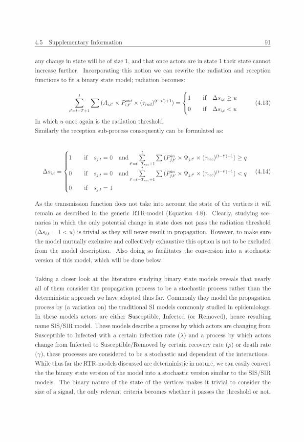
53_Erim_Vermeer Stand.job
4.5 Supplementary Information 91
any change in state will be of size 1, and that once actors are in state 1 their state cannot
increase further. Incorporating this notion we can rewrite the radiation and reception
functions to fit a binary state model; radiation becomes:
t∑t′=t−T+1
∑(Ai,t′ × P out
i,t′ × (τrad)(t−t′)+1) =
⎧⎨⎩1 if Δsi,t ≥ u
0 if Δsi,t < u(4.13)
In which u once again is the radiation threshold.
Similarly the reception sub-process consequently can be formulated as:
Δsi,t =
⎧⎪⎪⎪⎪⎪⎨⎪⎪⎪⎪⎪⎩
1 if sj,t = 0 andt∑
t′=t−Trec+1
∑(P in
j,t′ ×Ψj,t′ × (τrec)(t−t′)+1) ≥ q
0 if sj,t = 0 andt∑
t′=t−Trec+1
∑(P in
j,t′ ×Ψj,t′ × (τrec)(t−t′)+1) < q
0 if sj,t = 1
(4.14)
As the transmission function does not take into account the state of the vertices it will
remain as described in the generic RTR-model (Equation 4.8). Clearly, studying sce-
narios in which the only potential change in state does not pass the radiation threshold
(Δsi,t = 1 < u) is trivial as they will never result in propagation. However, to make sure
the model mutually exclusive and collectively exhaustive this option is not to be excluded
from the model description. Also doing so facilitates the conversion into a stochastic
version of this model, which will be done below.
Taking a closer look at the literature studying binary state models reveals that nearly
all of them consider the propagation process to be a stochastic process rather than the
deterministic approach we have adopted thus far. Commonly they model the propagation
process by (a variation on) the traditional SI models commonly studied in epidemiology.
In these models actors are either Susceptible, Infected (or Removed), hence resulting
name SIS/SIR model. These models describe a process by which actors are changing from
Susceptible to Infected with a certain infection rate (λ) and a process by which actors
change from Infected to Susceptible/Removed by certain recovery rate (ρ) or death rate
(γ), these processes are considered to be a stochastic and dependent of the interactions.
While thus far the RTR-models discussed are deterministic in nature, we can easily convert
the the binary state version of the model into a stochastic version similar to the SIS/SIR
models. The binary nature of the state of the vertices makes it trivial to consider the
size of a signal, the only relevant criteria becomes whether it passes the threshold or not.

53_Erim_Vermeer Stand.job
92 Study 1: The RTR-model of propagation
Therefore rather than considering size of a signal we can consider the probability that it
passes the threshold. This effectively changes the emphasis of the model from size (read
deterministic) to probabilities (read stochastic), facilitating the comparison of the RTR-
model to traditional SIS/SIR models.
This stochastic RTR-model resembles traditional SIS models but differs in two respects;
First it considers the local interaction, rather than the mean field level dynamics, and
second it includes the three sub-processes for propagation rather than a single process.
We consider there to be a probability of success for each of the sub-processes, and thus
decompose the propagation probability (λ) into three distinct probabilities (α, φ, η), one
for each sub-process. For each sub-process a likelihood that the signal is being forwarded to
the next stage of the propagation process can be included. Propagation can consequently
be modeled by means of three Bernoulli distributions. The first describes the probability
of successful Radiation (α), the second of successful Transmission (φ), and the third of
successful Reception (η). The general RTR-model in cases of binary vertex states can thus
be easily transformed into a stochastic variant in which we assume that some function of
the radiation/transmission/reception parameters, will yield a probability of it successfully
occurring.
In a stochastic version of the RTR-model the radiation likelihood describes the probability
that a change in state (which can only be of size 1) will be larger than the radiation
threshold, and thus yields any signal towards the outgoing edge(s). This probability
is only influenced by a function of the radiation properties (A∗i,t = f(Ai,t) = (α∗
i,e,t)|e ∈Eout
i,t = f(Ai,t)) of the actor sending the signal(i) and the memory in the system. Therefore
it can be formulated as:
pouti,e,t ∼ Bern(p) in which p = 1−t∏
t′=t−Trad+1
(1− (Δsi,t′ × α∗i,e,t′ × (τrad)
(t−t′)+1) (4.15)
The SIS/SIR models can be denoted as a special case of this general stochastic form. The
traditional SIS models make two assumptions; first it assumes no memory in the system,
second it assumes that radiation is caused by the state itself rather than the change of
this state (once an actor is sick it has a chance to radiate). These two assumptions allow
us to reduce equation 4.15 to:
pouti,e,t =
⎧⎨⎩∼ Bern(α∗
i,e,t) if si,t = 1
0 if si,t = 0(4.16)
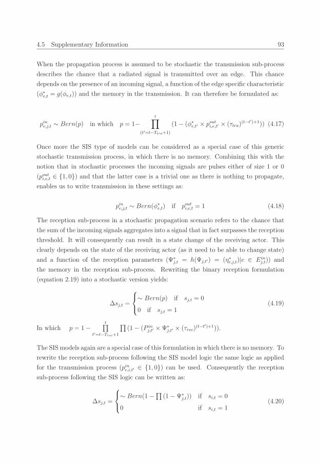
54_Erim_Vermeer Stand.job
4.5 Supplementary Information 93
When the propagation process is assumed to be stochastic the transmission sub-process
describes the chance that a radiated signal is transmitted over an edge. This chance
depends on the presence of an incoming signal, a function of the edge specific characteristic
(φ∗e,t = g(φe,t)) and the memory in the transmission. It can therefore be formulated as:
pine,j,t ∼ Bern(p) in which p = 1−t∏
(t′=t−Ttra+1)
(1− (φ∗e,t′ × pouti,e,t′ × (τtra)
(t−t′)+1)) (4.17)
Once more the SIS type of models can be considered as a special case of this generic
stochastic transmission process, in which there is no memory. Combining this with the
notion that in stochastic processes the incoming signals are pulses either of size 1 or 0
(pouti,e,t ∈ {1, 0}) and that the latter case is a trivial one as there is nothing to propagate,
enables us to write transmission in these settings as:
pine,j,t ∼ Bern(φ∗e,t) if pouti,e,t = 1 (4.18)
The reception sub-process in a stochastic propagation scenario refers to the chance that
the sum of the incoming signals aggregates into a signal that in fact surpasses the reception
threshold. It will consequently can result in a state change of the receiving actor. This
clearly depends on the state of the receiving actor (as it need to be able to change state)
and a function of the reception parameters (Ψ∗j,t = h(Ψj,t′) = (η∗e,j,t)|e ∈ Ein
j,t)) and
the memory in the reception sub-process. Rewriting the binary reception formulation
(equation 2.19) into a stochastic version yields:
Δsj,t =
⎧⎨⎩∼ Bern(p) if sj,t = 0
0 if sj,t = 1(4.19)
In which p = 1−t∏
t′=t−Trec+1
∏(1− (P in
j,t′ ×Ψ∗j,t′ × (τrec)
(t−t′)+1)).
The SIS models again are a special case of this formulation in which there is no memory. To
rewrite the reception sub-process following the SIS model logic the same logic as applied
for the transmission process (pine,i,t′ ∈ {1, 0}) can be used. Consequently the reception
sub-process following the SIS logic can be written as:
Δsj,t =
⎧⎨⎩∼ Bern(1−∏
(1−Ψ∗j,t)) if si,t = 0
0 if si,t = 1(4.20)
54_Erim_Vermeer Stand.job
94 Study 1: The RTR-model of propagation
S4: Brute-force fitting
During the first part of our study we use a brute-force simulation approach to reproduce
the actual propagation number found when considering the propagation of the Yahoo! Go
2.0 application. We distill the actual propagation and the network structure at the start
of our observation period from the data and use this information as the input for our set
of simulations. Given this starting scenario, we run a series of simulations in which we
vary the propagation mechanism, namely the radiation, transmission and reception pa-
rameters ((α, φ, η)). While many arbitrary heuristics could be used to find the optimal set
of parameters (radiation, transmission and reception probabilities), all of these heuristics
require sequential fitting, which in turn means that we have to include a prioritization in
the sequence in which each of the parameters is fitted. This prioritization might cause
the heuristic to get stuck in a local minimum, strongly biasing the fitting outcomes. To
circumvent this problem a brute-force simulation approach is used in this study.
The brute-force approach implies doing a complete sweep of the parameter space in order
to find the global minimum. As the RTR-model uses three distinct parameters, each
decimal added to the parameter estimation will increase the number of scenarios in the
parameter space by a factor of 1,000 (103). Therefore the brute-force approach has con-
siderable implications for the processing time, forcing a trade-off between scope and level
of detail. For this reason in the initial set of simulations a single decimal detail level
has been chosen. Resulting in 1,000 scenarios with different mechanisms (division into
Radiation, Transmission and Reception).
We simulate the stochastic propagation process on the given network structure (drawn
from the actual Yahoo! Go data) for each scenario with varying propagation parameters.
Using bootstrapping we run each scenario multiple times (5) and measure the average
amount of propagation (number of new adopters) per week in each scenario. We compare
these numbers to the numbers for adoption distilled from the actual data, and calculate
the fit between the simulated and actual propagation.
Fit measures
There exist many different potential fitting measures, three of them are used to calculate
fit in our study. First, we use the traditional root-mean-squared error (RMSE), and then,
because there are big variations in the absolute propagation numbers (the propagation
in the first week of observation is an order of magnitude bigger that the propagation in
the last week), we also include both the logged root-mean-square error (LRMSE) and the
relative root-mean-square error (RRMSE). These measures are formulated as follows:
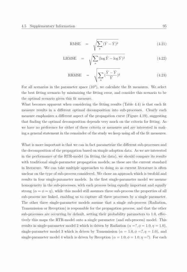
55_Erim_Vermeer Stand.job
4.5 Supplementary Information 95
RMSE =
√∑n
(Y − Y )2 (4.21)
LRMSE =
√∑n
(log Y − log Y )2 (4.22)
RRMSE =
√√√√∑n
(Y − Y
Y)2 (4.23)
For all scenarios in the parameter space (103), we calculate the fit measures. We select
the best fitting scenario by minimizing the fitting error, and consider this scenario to be
the optimal scenario given this fit measure.
What becomes apparent when considering the fitting results (Table 4.4) is that each fit
measure results in a different optimal decomposition into sub-processes. Clearly each
measure emphasizes a different aspect of the propagation curve (Figure 4.19), suggesting
that finding the optimal decomposition depends very much on the criteria for fitting. As
we have no preference for either of these criteria or measures and are interested in mak-
ing a general statement in the remainder of the study we keep using all of the fit measures.
What is more important is that we can in fact parametrize the different sub-processes and
the decomposition of the propagation based on simple adoption data. As we are interested
in the performance of the RTR-model (in fitting the data), we should compare its results
with traditional single-parameter propagation models, as these are the current standard
in literature. We can take multiple approaches to doing so as current literature is often
unclear on the type of sub-process considered. We chose an approach which is twofold and
results in four single-parameter models. In the first single-parameter model we assume
homogeneity in the sub-processes, with each process being equally important and equally
strong (α = φ = η), while this model still assumes three sub-process the properties of all
sub-process are linked, enabling us to capture all three processes by a single parameter.
The other three single-parameter models assume that a single sub-process (Radiation,
Transmission or Reception) is responsible for the propagation process, and that the other
sub-processes are occurring by default, setting their probability parameters to 1.0, effec-
tively this maps the RTR-model onto a single parameter (and sub-process) model. This
results in single-parameter model 2 which is driven by Radiation (α =?, φ = 1.0, η = 1.0),
single-parameter model 3 which is driven by Transmission (α = 1.0, φ =?, η = 1.0), and
single-parameter model 4 which is driven by Reception (α = 1.0, φ = 1.0, η =?). For each
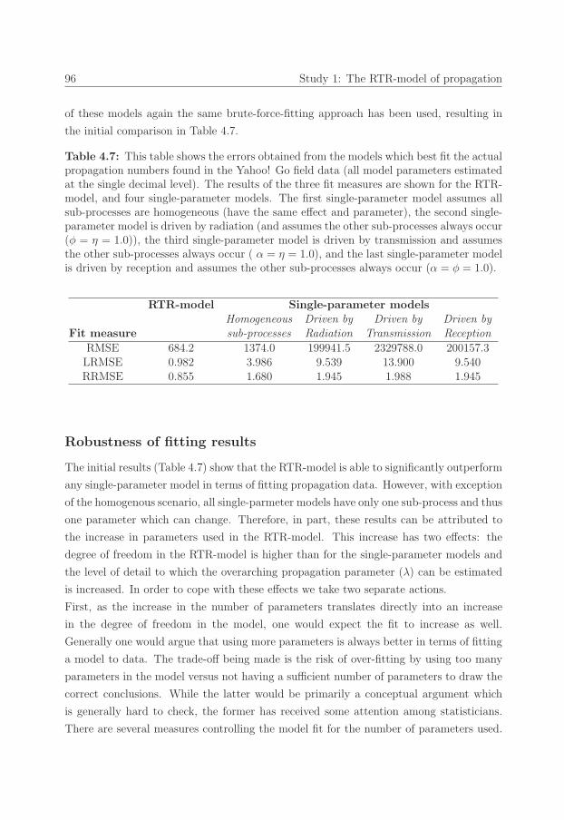
55_Erim_Vermeer Stand.job
96 Study 1: The RTR-model of propagation
of these models again the same brute-force-fitting approach has been used, resulting in
the initial comparison in Table 4.7.
Table 4.7: This table shows the errors obtained from the models which best fit the actualpropagation numbers found in the Yahoo! Go field data (all model parameters estimatedat the single decimal level). The results of the three fit measures are shown for the RTR-model, and four single-parameter models. The first single-parameter model assumes allsub-processes are homogeneous (have the same effect and parameter), the second single-parameter model is driven by radiation (and assumes the other sub-processes always occur(φ = η = 1.0)), the third single-parameter model is driven by transmission and assumesthe other sub-processes always occur ( α = η = 1.0), and the last single-parameter modelis driven by reception and assumes the other sub-processes always occur (α = φ = 1.0).
RTR-model Single-parameter modelsHomogeneous Driven by Driven by Driven by
Fit measure sub-processes Radiation Transmission Reception
RMSE 684.2 1374.0 199941.5 2329788.0 200157.3LRMSE 0.982 3.986 9.539 13.900 9.540RRMSE 0.855 1.680 1.945 1.988 1.945
Robustness of fitting results
The initial results (Table 4.7) show that the RTR-model is able to significantly outperform
any single-parameter model in terms of fitting propagation data. However, with exception
of the homogenous scenario, all single-parmeter models have only one sub-process and thus
one parameter which can change. Therefore, in part, these results can be attributed to
the increase in parameters used in the RTR-model. This increase has two effects: the
degree of freedom in the RTR-model is higher than for the single-parameter models and
the level of detail to which the overarching propagation parameter (λ) can be estimated
is increased. In order to cope with these effects we take two separate actions.
First, as the increase in the number of parameters translates directly into an increase
in the degree of freedom in the model, one would expect the fit to increase as well.
Generally one would argue that using more parameters is always better in terms of fitting
a model to data. The trade-off being made is the risk of over-fitting by using too many
parameters in the model versus not having a sufficient number of parameters to draw the
correct conclusions. While the latter would be primarily a conceptual argument which
is generally hard to check, the former has received some attention among statisticians.
There are several measures controlling the model fit for the number of parameters used.
56_Erim_Vermeer Stand.job
4.5 Supplementary Information 97
The Akaike information criterion (AIC) (Akaike, 1974) is one of the most commonly
used measures in this area. It penalizes for the number of parameters used to generate
the fitting error, and by doing so provides a more balanced way of comparing models
with varying numbers of parameters. As we are in fact comparing models with different
numbers of parameters we apply the AIC in order to give a more fair comparison and
reduce the risk of over-fitting.
Second, the increase in the number of parameters has a second effect: it increase the level
of detail. We divide the traditional propagation parameter into three distinct parameters,
and measure each on a single decimal detail level. Consequently we are comparing models
which describe the overall propagation parameter on a single decimal (which is the case
when we use a single-parameter model) with a model which can estimate the propagation
parameter at three decimals (one for each sub-process, 0.13). While AIC already controls
for this aspect, on top of this correction we increase the level of detail for the single-
parameter benchmark models (with exception of the homogenous scenario) by a factor
of 10. Consequently these models are estimated on the 0.01 parameter detail level when
compared to the RTR-model. The results of these corrections can be found in Table 4.5.
S5: Simulation using the RTR-model
In the second section of the paper the simulation model is used to show the impact of
dividing the propagation mechanism into the three sub-processes. To allow propagation
to be modeled some constraints are required, and a network has to be generated on which
to run the propagation process. In our simulations the following constraints are used:
• The state of an actor is either 1 (infected) or 0 (susceptible); the default is that
actors are susceptible
• The weight of all edges is equal and one, w(ij, t) = 1
• The edges are undirected, resulting effectively in a unweighted undirected network
• The number of nodes in the network is fixed, n = 10, 000
• Each node has on average three edges, m = 3
• The probability of recovering from a disease is fixed, ρ = 0.2
• The overarching propagation probability is fixed, λ = 0.192
• The propagation is initiated from a single seed
56_Erim_Vermeer Stand.job
98 Study 1: The RTR-model of propagation
• The simulation will run for 30 time-steps
As the starting point for the simulation, a single undirected scale-free network based on
the Barabasi-Albert Barabasi and Albert (1999) approach is generated, in which each
vertex has on average three (m = 3) edges. This structure remains constant over all
simulations, effectively removing any influence of network structure on the outcomes of
the simulation. An infection is introduced to the network by randomly selecting a seed
node and changing its state to Infected. This node starts radiating and thereby serves as
the seed of the infection, and consequently the propagation process with given mechanism
(pre-defined sub-process parameters) is simulated while the pervasiveness —the propor-
tion of the population which is infected— is tracked over time.
In order to generate robust results we use bootstrapping, effectively repeating the process
described above 100 times. The results are then averaged over this bootstrapped set of
simulations, resulting in a single pervasiveness curve for each propagation scenario.
Validating the RTR simulation model
In the first set of scenarios we investigate the notion that a propagation process can be
decomposed into sub-processes. While the chance of propagation has been conceptually
claimed to be a product of three consecutive stochastic processes, in the initial stage we
use simulation to test this claim. To do so we use a sample set of four scenarios where
the propagation probability is equal for in each case (λ1 = λ2 = λ3 = λ4 = 0.192).
These scenarios do differ in their mechanism, way in which they are decomposed into
sub-processes. Scenario 1 is a process with low radiation, medium transmission and high
reception (α = 0.4, φ = 0.6, η = 0.8); scenario 2 is a process with medium radiation, high
transmission and low reception (α = 0.6, φ = 0.8, η = 0.4); scenario 3 is a process with
high radiation, low transmission and medium reception (α = 0.8, φ = 0.4, η = 0.6); and
scenario 4 is a process in which the sub-processes are homogeneous (α = φ = η = 0.5769).
The initial results (Figure 4.20) show variations in propagation outcomes for these dif-
ferent scenarios; based on the conceptual decomposition argument, one would, however,
expect there to be no differences between these models.
Further investigation (Figure 4.21) revealed that the variations found are in fact insignif-
icant, which indicates that the limited amount of the bootstrapping might have caused
the differences in the initial results. As these results were generated using a set of 100
bootstrapped simulations it is likely that variations have risen from either stochasticity or
57_Erim_Vermeer Stand.job
4.5 Supplementary Information 99
sampling, causing differences in local structure surrounding the seed of infection. There-
fore a second set of simulations has been run in which each node in the population is
used as seed nodes. In this set of simulations each node is chosen once as the seed of
infection. This resulted in a bootstrapped sample of 10,000 simulations —the increased
sample size should reduce the stochastic problems— in which each actor has been used
as seed node, removing all potential sampling bias. The simulation results (Figure 4.22)
show that the pervasiveness curves for the three scenarios lie exactly on top of each other,
confirming two things. First, it indicates that variation in propagation process outcomes
can occur due to sampling and/or stochasticity, which has important implications for the
generalization of propagation process outcomes, and supporting the notion that the seed
plays a role in the eventual outcomes of propagation process (something which outside
the scope of this paper). Second, it shows that on the mean-field all four scenarios yield
a similar pervasiveness, supporting the notion that a propagation process can indeed be
decomposed into three distinct sub-processes.
Simulating interventions using the RTR-model
We have shown that decomposing the propagation process into three sub-processes is both
methodologically desirable, and conceptually valid. This allows us to use the RTR-model
to simulate the impact of interventions in the propagation process. Once more the same
four scenarios are used during the simulation of the interventions. We compare scenarios
with different mechanisms (and corresponding decompositions) but similar propagation
probabilities (λ). An intervention is included in the simulation by changing a single prop-
agation parameter (either α, φ or η) during the simulation. We extend the number of
time-steps (t) to 100, and at t = 50 a parameter of one of the sub-processes is reduced
by the arbitrary amount of 0.2, which effectively means that the chance that this sub-
process will take place successfully (i.e. result in a signal) is decreased by 20%. To avoid
potential stochasticity or selection bias, the scenarios are once more bootstrapped 10,000
times, once for each potential starting seed.
Our simulations show the results of interventions in each of the sub-processes: radiation
(Figure 4.3), transmission (Figure 4.4), and reception (Figure 4.2). Two things become
apparent from these simulations.
First and foremost, these results support the notion that the mechanism of the propa-
gation process plays a critical role in determining the effect of an intervention on the
dynamics of the propagation process. As interventions are aimed only at changing the
parameter of a single sub-process, our simulations show that to model the effect of such
57_Erim_Vermeer Stand.job
100 Study 1: The RTR-model of propagation
interventions effectively one needs to be able to break down the propagation process into
the sub-processes. Only once this decomposition is known can one estimate the impact
of an intervention.
Second, the effectiveness of interventions varies a great deal, depending on the decompo-
sition into sub-processes. This becomes even more apparent when we considering Figures
4.5,4.6,4.7 and 4.8 which capture the same adoption curse, but represent it per mechanism,
consequently each line represents a distinct intervention ( in either Radiation, Transmis-
sion or Reception). Scenario 1 is depicted in Figure 4.5, scenario 2 can be found in Figure
4.6, scenario 3 in Figure 4.7 and scenario 4 in Figure 4.8. When we consider scenario 4
(Figure 4.8), we find all interventions (in any single sub-process) to have an equal effect.
Therefore in this specific scenario —which assumes homogenous sub-processes— any in-
tervention will have the same effect, and consequently the distinction in sub-processes
seems to bear no additional value. The remainder of the figures however show that there
are differences between different decompositions when it comes to the effectiveness of in-
terventions.
To get a feel for the extent to which these differences lead to over- or underestimation of
intervention effects we take a closer look at some extreme scenarios. We again take the
scenario with homogeneous sub-processes (scenario 4) as our benchmark, as this scenario
fits the current state of most propagation research. We compare this scenario to two
extreme scenarios: scenario 5, the ‘worst case’ most resilient scenario in which the param-
eter under intervention is initially maximized (1.0), and scenario 6, the ‘best case’ most
volatile scenario in which the parameter under intervention is equal to the intervention
size (0.2). The results of these simulations (Table 4.3, Figure 4.9) show that both under-
and overestimation of the intervention effect are possible. In this specific example setting,
based on the default scenario (scenario 4) one would expect a reduction in pervasive-
ness of 12.7%. In the most resilient scenario (scenario 5), one can see that pervasiveness
is, however, only reduced by 6.1%, so by assuming sub-processes to be homogeneous one
could overestimate the effectiveness of this intervention by 52.0%. In contrast, in the most
volatile scenario (scenario 6), the infection is completely removed. The pervasiveness is
thus reduced by 100%, indicating that in this case if one had used the default scenario
the intervention effect would have been underestimated by 687.4%.

58_Erim_Vermeer Stand.job
4.5 Supplementary Information 101
0 20 40 60 80 100
0.0
0.2
0.4
0.6
0.8
1.0
Time
Per
vasi
vene
ss
● ●●
●
●
●
●
●
●
●
●
●● ● ● ● ● ● ● ● ● ● ● ● ● ● ● ● ● ● ● ● ● ● ● ● ● ● ● ● ● ● ● ● ● ● ● ● ●
●
●
●●
● ● ● ● ● ● ● ● ● ● ● ● ● ● ● ● ● ● ● ● ● ● ● ● ● ● ● ● ● ● ● ● ● ● ● ● ● ● ● ● ● ● ● ● ● ● ●
● Scenario 1: Radiation=0.4, Transmission=0.6 , Reception=0.8 Scenario 2: Radiation=0.6, Transmission=0.8 , Reception=0.4 Scenario 3: Radiation=0.8, Transmission=0.4 , Reception=0.6 Scenario 4: Radiation=Transmission=Reception=0.5769
Figure 4.3: The pervasiveness over time is depicted for scenarios with the same overar-ching propagation likelihood (λ = 0.192) but with different decompositions into radiation(α), transmission (φ) and reception (η). The black open circles represent a process withα = 0.4, φ = 0.6 and η = 0.8. The green pluses represent a process with α = 0.6, φ =0.8 and η = 0.4. The (grey) triangles represent a process with α = 0.8, φ = 0.4 and η= 0.6. The blue crosses represent a process with homogeneous sub-processes (α = φ =η = 0.5769). During the simulation at t = 50 an intervention (reduction of 0.2) in theradiation is applied

58_Erim_Vermeer Stand.job
102 Study 1: The RTR-model of propagation
0 20 40 60 80 100
0.0
0.2
0.4
0.6
0.8
1.0
Time
Per
vasi
vene
ss
● ●●
●
●
●
●
●
●
●
●
●● ● ● ● ● ● ● ● ● ● ● ● ● ● ● ● ● ● ● ● ● ● ● ● ● ● ● ● ● ● ● ● ● ● ● ● ●
●
●● ● ● ● ● ● ● ● ● ● ● ● ● ● ● ● ● ● ● ● ● ● ● ● ● ● ● ● ● ● ● ● ● ● ● ● ● ● ● ● ● ● ● ● ● ● ● ● ●
● Scenario 1: Radiation=0.4, Transmission=0.6 , Reception=0.8 Scenario 2: Radiation=0.6, Transmission=0.8 , Reception=0.4 Scenario 3: Radiation=0.8, Transmission=0.4 , Reception=0.6 Scenario 4: Radiation=Transmission=Reception=0.5769
Figure 4.4: The pervasiveness over time is depicted for scenarios with the same overar-ching propagation likelihood (λ = 0.192) but with different decompositions into radiation(α), transmission (φ) and reception (η). The black open circles represent a process withα = 0.4, φ = 0.6 and η = 0.8. The green pluses represent a process with α = 0.6, φ =0.8 and η = 0.4. The (grey) triangles represent a process with α = 0.8, φ = 0.4 and η= 0.6. The blue crosses represent a process with homogeneous sub-processes (α = φ =η = 0.5769). During the simulation at t = 50 an intervention (reduction of 0.2) in thetransmission is applied

59_Erim_Vermeer Stand.job
4.5 Supplementary Information 103
0 20 40 60 80 100
0.0
0.2
0.4
0.6
0.8
1.0
Scenario 1: Radiation=0.4, Transmission=0.6 , Reception=0.8
Time
Per
vasi
vene
ss
● ●●
●
●
●
●
●
●
●
●
●● ● ● ● ● ● ● ● ● ● ● ● ● ● ● ● ● ● ● ● ● ● ● ● ● ● ● ● ● ● ● ● ● ● ● ● ●
●
●
●●
● ● ● ● ● ● ● ● ● ● ● ● ● ● ● ● ● ● ● ● ● ● ● ● ● ● ● ● ● ● ● ● ● ● ● ● ● ● ● ● ● ● ● ● ● ● ●
● Intervention in the Radiation sub−process Intervention in the Transmission sub−processIntervention in the Reception sub−process
Figure 4.5: The pervasiveness over time is depicted for scenario 1 which is characterizedby a propagation process with α = 0.4, φ = 0.6 and η = 0.8. Different interventions(-0.2) are applied in this scenario; the black open circles represent an intervention inthe radiation parameter, the green pluses represent an intervention in the transmissionparameter and the grey triangles represent an intervention in the reception parameter.

59_Erim_Vermeer Stand.job
104 Study 1: The RTR-model of propagation
0 20 40 60 80 100
0.0
0.2
0.4
0.6
0.8
1.0
Scenario 2: Radiation=0.6, Transmission=0.8 , Reception=0.4
Time
Per
vasi
vene
ss
● ●●
●
●
●
●
●
●
●
●●
● ● ● ● ● ● ● ● ● ● ● ● ● ● ● ● ● ● ● ● ● ● ● ● ● ● ● ● ● ● ● ● ● ● ● ● ●
●
●● ● ● ● ● ● ● ● ● ● ● ● ● ● ● ● ● ● ● ● ● ● ● ● ● ● ● ● ● ● ● ● ● ● ● ● ● ● ● ● ● ● ● ● ● ● ● ● ●
● Intervention in the Radiation sub−process Intervention in the Transmission sub−processIntervention in the Reception sub−process
Figure 4.6: The pervasiveness over time is depicted for scenario 2 which is characterizedby a propagation process with α = 0.6 , φ = 0.8 and η = 0.4. Different interventions(-0.2) are applied in this scenario; the black open circles represent an intervention inthe radiation parameter, the green pluses represent an intervention in the transmissionparameter and the grey triangles represent an intervention in the reception parameter.

60_Erim_Vermeer Stand.job
4.5 Supplementary Information 105
0 20 40 60 80 100
0.0
0.2
0.4
0.6
0.8
1.0
Scenario 3: Radiation=0.8, Transmission=0.4 , Reception=0.6
Time
Per
vasi
vene
ss
● ●●
●
●
●
●
●
●
●
●
●● ● ● ● ● ● ● ● ● ● ● ● ● ● ● ● ● ● ● ● ● ● ● ● ● ● ● ● ● ● ● ● ● ● ● ● ●
●● ● ● ● ● ● ● ● ● ● ● ● ● ● ● ● ● ● ● ● ● ● ● ● ● ● ● ● ● ● ● ● ● ● ● ● ● ● ● ● ● ● ● ● ● ● ● ● ● ●
● Intervention in the Radiation sub−process Intervention in the Transmission sub−processIntervention in the Reception sub−process
Figure 4.7: The pervasiveness over time is depicted for scenario 3 which is characterizedby a propagation process with α = 0.8 , φ = 0.4 and η = 0.6. Different interventions(-0.2) are applied in this scenario; the black open circles represent an intervention inthe radiation parameter, the green pluses represent an intervention in the transmissionparameter and the grey triangles represent an intervention in the reception parameter.

60_Erim_Vermeer Stand.job
106 Study 1: The RTR-model of propagation
0 20 40 60 80 100
0.0
0.2
0.4
0.6
0.8
1.0
Scenario 4: Radiation=Transmission=Reception=0.5769
Time
Per
vasi
vene
ss
● ●●
●
●
●
●
●
●
●
●
●● ● ● ● ● ● ● ● ● ● ● ● ● ● ● ● ● ● ● ● ● ● ● ● ● ● ● ● ● ● ● ● ● ● ● ● ●
●
●● ● ● ● ● ● ● ● ● ● ● ● ● ● ● ● ● ● ● ● ● ● ● ● ● ● ● ● ● ● ● ● ● ● ● ● ● ● ● ● ● ● ● ● ● ● ● ● ●
● Intervention in the Radiation sub−process Intervention in the Transmission sub−processIntervention in the Reception sub−process
Figure 4.8: The pervasiveness over time is depicted for scenario 4 which is characterizedby a propagation process in which sub-processes are homogeneous (α = φ = η = 0.5769).Different interventions (-0.2) are applied in this scenario; the black open circles representan intervention in the radiation parameter, the green pluses represent an interventionin the transmission parameter and the grey triangles represent an intervention in thereception parameter.

61_Erim_Vermeer Stand.job
4.5 Supplementary Information 107
0 20 40 60 80 100
0.0
0.2
0.4
0.6
0.8
1.0
Time
Per
vasi
vene
ss
● ●●
●
●
●
●
●
●
●
●
●● ● ● ● ● ● ● ● ● ● ● ● ● ● ● ● ● ● ● ● ● ● ● ● ● ● ● ● ● ● ● ● ● ● ● ● ●
●
●● ● ● ● ● ● ● ● ● ● ● ● ● ● ● ● ● ● ● ● ● ● ● ● ● ● ● ● ● ● ● ● ● ● ● ● ● ● ● ● ● ● ● ● ● ● ● ● ●
● Scenario 4: Radiation=Transmission=Reception=0.5769Scenario 5: Radiation=0.192, Transmission=1.0 , Reception=1.0Scenario 6: Radiation=0.1, Transmission=0.96 , Reception=0.2
Figure 4.9: The pervasiveness over time is depicted under an intervention in the re-ception (η). Three scenarios are depicted: scenario 4 (black open circles) which hashomogeneous sub-processes (α = φ = η = 0.5769), scenario 5 (grey triangles) in whichthe intervened parameter was initially maximized(pre-intervention: η = 1.0), and scenario6 (green pluses) in which the intervened parameter was initially equal to the interventionsize (pre-intervention: η = 0.2)
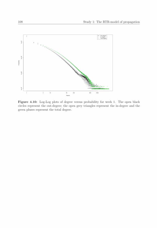
61_Erim_Vermeer Stand.job
108 Study 1: The RTR-model of propagation
1 5 10 50 100 500 1000
1e−
071e−
051e−
031e−
01
Degree
Pro
babi
lity
●
●
●
●
●
●●
●●
●●
●●
●●●●●●●●
●●●●●●●●●
●●●●●●
●●●●●●●●●●●●●●●●●●●●●●●●●●●●●●●●●●●●●●●●●●●●●●●●●
●●●●●●●●
●●●●●●●●●●●●●●●●●●●●●●
●●●●●●●●●●●
●●●●●●●●●●●●●●●●●●●●●
●
●●●●●●●●
●●
●●●●●●●●●●●●●●●●●●●●
●●●●●
●
●●●●●
●●●●●●●
●
●●●
●
●
●●
●●
●
●●●●●●●
●●●
●●●●●●●
●
●●●●●●●
●●●●●●
●●
●
●●●●●●●●●
●●●●●●●●●●●●●●●●●●●●
●●●●●
●
●●●
●●
●
●●●●●●●●
●
●●
●●●●
●
●●●●●
●●●●●
●●
●●
●
●
●●●●●
●
●●●
●
●
●●●
●
●●●●●●●●
●●●●●
●●●
●●
●
●●
●
●
●
●
●
●
●
●●
●●●
●
●
●
●●
●●●
●
●
●●●●●●
●
●●
●●
●
●●
●●●●●●●●●●
●●●●
●
●●●
●
●●●●
●●
●
●
●
●●
●
●
●
●
●●
●
●
●●
●
●
●●●
●
●
●
●
●
●
●
●
●●●
●
●●
●●
●
●
●
●●
●●
●
●
●
●
●
●
●
●●
●●
●
●●
●
●
●
●●
●
●
●
●
●
●
●●
●●
●
●
●
●
●
●
●●
●
●
●
●●
●
●
●
●●●
●
●●
●●
●●●
●
●
●
●
●
●●
●
●
●
●
●
●
●
●
●●
●
●
●●
●
●
●●
●
●●●
●●
●●
●●
●
●●●
●
●●●●●●
●
●●
●
●●
●
●●●
●
●
●
●
●
●●
●
●●●
●
●
●
●
●●●
●
●●●
●
●●●●●●
●●
●
●●●●●●●
●●●
●●●●●●●●●●
●●●●
●
●
●●
●
●●●●●●●
●
●●●
●
●●
●
●●●
●●
●●●●●●●●●●●●
●
●●●●●●●●
●
●●●●
●●
●●●●●●●
●
●●●●●●●●●●●
●
●●●●●●●●●●●●●●
●
●
●●
●●●●●●●●●●●●●●●●●●●●●●●●●●●●●●●●●●●●●●●●●●●● ●
● Out−degreeIn−degreeTotal degree
Figure 4.10: Log-Log plots of degree versus probability for week 1. The open blackcircles represent the out-degree; the open grey triangles represent the in-degree and thegreen pluses represent the total degree.
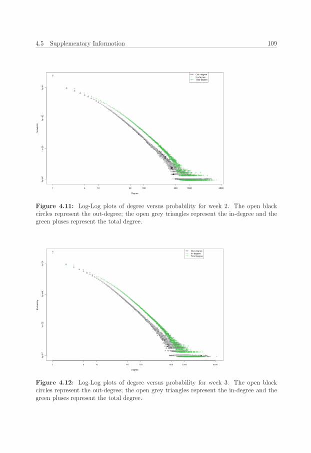
62_Erim_Vermeer Stand.job
4.5 Supplementary Information 109
1 5 10 50 100 500 1000 5000
1e−
071e−
051e−
031e−
01
Degree
Pro
babi
lity
●
●
●
●
●●
●●
●●
●●
●●
●●●●●●●●●●●●
●●●●●●●●●●●●●●●●●●●●●●●●●●●●●●●●●●●●●●●●●●●●●●●●●●●●●●●●●●●●●●●●●●●●●●●●
●●●●●●●●●●●●●●●●●●●●●●●●●●●●●●●●●●●●●●●●●●●●●●
●●●●●●●●●●●●●●●●●
●●●●●●●●●●●●●
●●●●●●●●●●●●●●●●●●●
●●●●●
●●●●●●
●●●
●●●●●●●●●●●●●●●●●
●
●●
●
●
●●●●●●
●●
●
●●●●
●
●●●●●●●●
●●●●●●
●●●●●●●●●●●●
●
●●
●
●●
●
●●●●
●
●
●
●
●●●●●●●●●
●
●●
●●●
●●●●
●
●
●●●●
●
●●
●●●●●●
●
●●●●●●●
●
●
●●
●
●●●●
●
●●●●
●
●●●●
●
●
●
●●●
●
●●●
●●
●
●●
●
●
●●●●
●
●●●
●●
●
●
●
●
●
●
●
●●
●●
●●
●●
●●●
●
●
●
●
●
●●
●●
●
●●●
●
●
●●
●●●●
●
●●
●●●●
●●●
●
●
●
●●
●●●●●
●
●
●
●
●
●
●
●
●
●
●
●●
●
●
●
●●
●
●
●
●
●
●
●
●●
●
●
●●
●
●
●
●
●●●●●●
●
●
●●
●
●
●
●
●
●●●
●●●
●
●●●
●
●
●
●
●
●
●
●
●●
●
●●
●
●●
●
●
●●
●
●●
●
●
●
●
●●
●●
●●
●
●
●
●
●●
●
●
●
●
●
●
●●
●●
●●
●
●
●
●
●
●
●
●
●
●
●
●●●
●●●
●
●
●●
●
●
●
●●
●
●
●
●
●
●
●
●
●●
●
●
●
●
●
●
●●
●
●●●●
●
●●
●
●
●●●
●
●
●
●●
●
●●
●
●●●●●●●
●
●●
●
●
●
●
●
●
●
●●
●●
●●●●●●●
●
●●●
●
●●●●●●●
●
●
●
●
●●●●●●●●●●
●
●●●
●●
●●
●●
●
●
●●●●
●
●●
●
●
●
●
●●
●
●
●
●●●●●
●
●●●●
●●●
●●●●●●●●●●●●●●●●
●
●●
●
●
●●
●
●
●●●●●
●
●●
●
●
●●●●●●●●●●●●●●●
●
●●●●●●●
●
●●●●
●
●●●●●●●●●●●●●●●●●●●●●●●●●●●●●●● ●●●●●●● ● ●●●●●●●● ●
● Out−degreeIn−degreeTotal degree
Figure 4.11: Log-Log plots of degree versus probability for week 2. The open blackcircles represent the out-degree; the open grey triangles represent the in-degree and thegreen pluses represent the total degree.
1 5 10 50 100 500 1000 5000
1e−
071e−
051e−
031e−
01
Degree
Pro
babi
lity
●
●
●
●
●●
●●
●●
●●
●●●●●●●●●●
●●●●●●●●●●●●●●●●●●●●●●●●●●●●●●●●●●●●●●●●●●●●●●●●●●●●●●●●●●●●●●●●●●●●●●●●●●●●●●●●●●●●●●●●●●●●●●●●●●●●●●●●●●●●●●●●●●●
●
●●●●●●●●●●●●●●●●●●●●●●●●●●●●
●●●●●●●●●●
●
●●●●●●
●●●●●●●●
●●●●●●●●●●●●●●●●●
●
●●●
●
●●●●●●●●●●●●●●
●●●●
●
●
●●●●
●
●●
●
●
●
●
●●●●●
●●●●
●
●●●●
●●●●●●●●●●●
●
●●●
●
●●●●●
●
●
●●
●
●
●●●
●
●●●●●●
●●●●●●●
●
●
●
●
●
●●
●
●
●
●●
●●
●●
●●
●●●●●
●
●●
●●
●
●
●●
●
●●
●
●
●●●●●
●●
●
●●●●●
●●
●
●
●
●
●
●●
●
●
●●●
●
●●
●●
●
●
●●●
●
●
●
●●
●●
●
●
●
●
●●●●
●●
●
●●●
●
●
●
●
●●●●●●
●●
●
●●●
●
●●●●
●
●
●●●●
●
●
●●●●
●
●
●
●●●
●
●
●
●
●
●
●
●●
●
●●●●
●
●●●
●
●
●
●
●
●●●●
●
●●
●
●
●
●●
●●
●
●
●
●
●●
●●●●
●
●
●
●
●
●
●
●●●
●
●
●
●
●
●●
●
●
●
●●
●
●
●
●
●
●
●●
●
●
●
●
●
●
●
●●
●
●
●●
●
●
●
●
●●
●
●●
●
●
●
●
●
●●
●●
●
●
●●
●
●●
●
●
●
●●
●
●
●
●●●
●
●
●
●
●
●
●●
●●
●
●
●
●
●
●
●●●
●
●●●
●
●
●●
●
●
●
●
●●●
●●
●
●
●
●
●
●
●
●
●●
●
●●
●
●●
●
●●●
●●
●●
●●●●●●
●
●
●●
●
●●
●
●
●
●
●●
●
●
●
●●
●
●
●●
●●
●●●●●●
●
●
●
●
●●
●
●●
●●
●●●●
●●
●
●
●●
●
●●●●
●
●●
●
●●●
●
●
●
●
●●●●
●
●
●
●
●
●
●
●
●●
●●
●
●●
●
●●●●
●●
●●●●●●
●
●
●
●
●●●●
●
●●●●
●
●
●
●●
●
●●●●●
●
●
●
●●
●
●
●
●
●●●●●●
●
●●
●
●●●●●●●
●
●
●
●
●
●●●●●●●●●●●
●
●●●
●●
●●
●
●●●
●
●
●
●●●●●●●●●●●●●
●
●●●●●●●●●●
●
●●●●●●●●●
●
●●●●●●●●●●●
●
●●●●●●●●
●
●●●●●●
●
●●●●●●●●●●●●●●●●●●●●●●●●●●●●●●●●●●●●●●●●●●●● ●●●●●●●●●●●● ●● ●●●
● Out−degreeIn−degreeTotal degree
Figure 4.12: Log-Log plots of degree versus probability for week 3. The open blackcircles represent the out-degree; the open grey triangles represent the in-degree and thegreen pluses represent the total degree.

62_Erim_Vermeer Stand.job
110 Study 1: The RTR-model of propagation
1 5 10 50 100 500 1000 5000
1e−
071e−
051e−
031e−
01
Degree
Pro
babi
lity
●
●
●
●
●●
●●
●●
●●
●●●●●●●●●●●
●●●●●●●●●●
●●●●●●●●●●●●●●●●●●●●●●●●●●●●●●●●●●●●●●●●●●●●●●●●●●●●●●●●●●●●●●●●●●●●●●●●●●●●●
●●●●●●●●●●●●●●●●●●●●●●●●●●●●●●●●●●●●●●●●●●●●●●●●●●●●●●●●●●●●●●●●●●●●●●●
●●●●●●●●●
●●●●●●●●●●●●
●●●●●●
●
●●●●●●
●●
●●●●●●●●
●
●●●●●●●●●●●●●●●●●●●
●
●
●
●
●●●●●●●
●
●●●●●●●●●●●●●●●
●●●●
●●●●
●●●●●
●
●●●●
●
●
●●●●
●
●
●
●
●●
●
●●●●●
●●●
●●●●
●
●●●●
●
●
●
●
●●●●●●●●●●
●
●
●
●●
●●
●
●
●
●
●
●
●
●
●
●
●
●●●
●
●
●
●
●●
●●
●
●
●
●●●
●
●●
●●●
●
●
●
●●
●
●●●●
●
●
●
●
●●
●
●●
●●
●
●
●●
●
●●
●
●●●
●
●
●
●●
●
●
●●
●
●
●●
●
●
●
●
●
●
●
●
●
●
●
●●
●●
●●●
●●
●
●
●
●●
●
●
●
●
●
●
●
●
●
●●
●
●●
●●
●
●●
●
●
●
●
●
●●
●
●
●●
●
●●●
●
●●
●
●●
●●
●
●
●
●
●
●●
●
●
●
●●
●
●
●
●
●
●
●
●
●●
●
●
●
●
●●●
●●●●
●
●
●●●
●
●
●
●
●
●●
●
●
●
●
●
●●●●●●
●
●
●●
●
●●●
●
●●
●
●
●
●
●
●
●
●
●●●
●●●
●●
●
●
●
●
●
●
●
●
●
●
●
●
●
●
●
●
●
●
●●●
●
●
●
●
●
●
●
●
●●
●
●
●
●●●●
●
●
●
●●
●
●
●●
●●●●●●
●
●
●
●
●
●●●
●
●
●●●●●
●●
●●●
●
●●●●●
●
●
●
●
●●
●●●●●
●●
●
●
●●●●●●
●
●
●●●●●
●
●
●
●●●●
●
●●●●●
●
●
●
●●
●
●●
●
●
●
●●
●
●●●●
●
●●
●
●●●●
●
●●●●●●●●●●
●
●●●●●●●
●
●●●●●●●●
●
●●●●●●●●●●●●●
●
●●●●●●●●●●●●●●●●●●●●●●●●●●●●●●●●●●●
●
●●●●
●
●●●●●●●●●●●●●
●
●●●●●●●●●●●●●●●●●●●●●●●●●●●●●● ● ●
● Out−degreeIn−degreeTotal degree
Figure 4.13: Log-Log plots of degree versus probability for week 4. The open blackcircles represent the out-degree; the open grey triangles represent the in-degree and thegreen pluses represent the total degree.

63_Erim_Vermeer Stand.job
4.5 Supplementary Information 111
Figure 4.14: Log-Log plot of the In-Out degree correlations for week 1.
Figure 4.15: Log-Log plot of the In-Out degree correlations for week 2.

63_Erim_Vermeer Stand.job
112 Study 1: The RTR-model of propagation
Figure 4.16: Log-Log plot of the In-Out degree correlations for week 3.
Figure 4.17: Log-Log plot of the In-Out degree correlations for week 4.
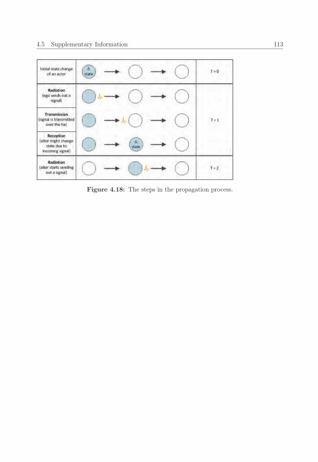
64_Erim_Vermeer Stand.job
4.5 Supplementary Information 113
Figure 4.18: The steps in the propagation process.

64_Erim_Vermeer Stand.job
114 Study 1: The RTR-model of propagation
Figure 4.19: This figure shows the number of new adopters over time due to prop-agation for the actual data (solid blue line), the best fitting decomposition using theRoot-Mean-Squared- Error (RMSE) fit measure (short-dashed green line), the best fit-ting decomposition using Logged-Root-Means-Squared-Error (LRMSE) measure (dottedblack line), and the best fitting decomposition using the Relative-Root-Mean-Squared-Error (RRMSE) measure (long dashed red line)

65_Erim_Vermeer Stand.job
4.5 Supplementary Information 115
0 20 40 60 80 100
0.0
0.2
0.4
0.6
0.8
1.0
Time
Per
vasi
vene
ss
● ●●
●
●
●
●
●
●
●
●●
● ● ● ● ● ● ● ● ● ● ● ● ● ● ● ● ● ● ● ● ● ● ● ● ● ● ● ● ● ● ● ● ● ● ● ● ● ● ● ● ● ● ● ● ● ● ● ● ● ● ● ● ● ● ● ● ● ● ● ● ● ● ● ● ● ● ● ● ● ● ● ● ● ● ● ● ● ● ● ● ● ● ● ● ● ● ● ●
● Scenario 1: Radiation=0.4, Transmission=0.6 , Reception=0.8 Scenario 2: Radiation=0.6, Transmission=0.8 , Reception=0.4 Scenario 3: Radiation=0.8, Transmission=0.4 , Reception=0.6 Scenario 4: Radiation=Transmission=Reception=0.5769
Figure 4.20: The pervasiveness over time is depicted for scenarios with the same prop-agation likelihood (λ = 0.192) but different divisions into radiation (α), transmission (φ)and reception (η). Scenario 1 (black open circles) represent a process with α = 0.4, φ =0.6, η = 0.8. Scenario 2 (grey triangles) represent a process with α = 0.6, φ = 0.8, η = 0.4.Scenario 3 (green pluses) represent a process with α = 0.8, φ = 0.4, η = 0.6. Scenario 4(blue crosses) represent a process with α = φ = η = 0.5769. Results are generated usinga bootstrapping sample (100 times) with a randomly selected seed node.
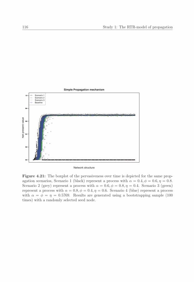
65_Erim_Vermeer Stand.job
116 Study 1: The RTR-model of propagation
●●●●●● ●●●●●●●
●●
●
●
●●●●●●● ●
●●●●●●●
●
●
●
●
●
●●●●
●
●
●●●
●
●
●
●
●
●
●
●●
●
●
●●●●●●●●●●●●●●●●●●● ●●
●
●●●●●●●●●●●●●●●●●
●
●●
●
●●●●●●●●●●●●●●●●● ●●
●
●●●●●●●●●●●●●●●●● ●●
●
●●●●●●●●●●●●●●●●● ●●●●●●●●●●●●●●●●
●
●● ●●●●●●●●●●●●●●●●
●
●● ●●●●●●●●●●●●●●●●
●
●● ●●●●●●●●●●●●●●●●
●
●● ●●●●●●●●●●●●●●●●
●
●● ●●●●●●●●●●●●●●●●
●
●● ●●●●●●●●●●●●●●●●●● ●●●●●●●●●●●●●●●●●● ●●●●●●●●●●●●●●●●●● ●●●●●●●●●●●●●●●●●● ●●●●●●●●●●●●●●●●●● ●●●●●●●●●●●●●●●●●● ●●●●●●●●●●●●●●●●●● ●●●●●●●●●●●●●●●●●● ●●●●●●●●●●●●●●●●●● ●●●●●●●●●●●●●●●●●● ●●●●●●●●●●●●●●●●●● ●●●●●●●●●●●●●●●●●● ●●●●●●●●●●●●●●●●●● ●●●●●●●●●●●●●●●●●● ●●●●●●●●●●●●●●●●●● ●●●●●●●●●●●●●●●●●● ●●●●●●●●●●●●●●●●●● ●●●●●●●●●●●●●●●●●● ●●●●●●●●●●●●●●●●●● ●●●●●●●●●●●●●●●●●● ●●●●●●●●●●●●●●●●●● ●●●●●●●●●●●●●●●●●● ●●●●●●●●●●●●●●●●●● ●●●●●●●●●●●●●●●●●● ●●●●●●●●●●●●●●●●●● ●●●●●●●●●●●●●●●●●● ●●●●●●●●●●●●●●●●●● ●●●●●●●●●●●●●●●●●● ●●●●●●●●●●●●●●●●●● ●●●●●●●●●●●●●●●●●● ●●●●●●●●●●●●●●●●●● ●●●●●●●●●●●●●●●●●● ●●●●●●●●●●●●●●●●●● ●●●●●●●●●●●●●●●●●● ●●●●●●●●●●●●●●●●●● ●●●●●●●●●●●●●●●●●● ●●●●●●●●●●●●●●●●●● ●●●●●●●●●●●●●●●●●● ●●●●●●●●●●●●●●●●●● ●●●●●●●●●●●●●●●●●● ●●●●●●●●
●
●●●●●●●●●● ●●●●●●●●●●●●●●●●●● ●●●●●●●●●●●●●●●●●● ●●●●●●●●●●●●●●●●●● ●●●●●●●●●●●●●●●●●● ●●●●●●●●●●●●●●●●●● ●●●●●●●●●●●●●●●●●● ●●●●●●●●●●●●●●●●●● ●●●●●●●●●●●●●●●●●● ●●●●●●●●●●●●●●●●●● ●●●●●●●●●●●●●●●●●● ●●●●●●●●●●●●●●●●●● ●●●●●●●●●●●●●●●●●● ●●●●●●●●●●●●●●●●●● ●●●●●●●●●●●●●●●●●● ●●●●●●●●●●●●●●●●●● ●●●●●●●●●●●●●●●●●● ●●●●●●●●●●●●●●●●●● ●●●●●●●●●●●●●●●●●● ●●●●●●●●●●●●●●●●●● ●●●●●●●●●●●●●●●●●● ●●●●●●●●●●●●●●●●●● ●●●●●●●●●●●●●●●●●● ●●●●●●●●●●●●●●●●●● ●●●●●●●●●●●●●●●●●● ●●●●●●●●●●●●●●●●●● ●●●●●●●●●●●●●●●●●● ●●●●●●●●●●●●●●●●●● ●●●●●●●●●●●●●●●●●● ●●●●●●●●●●●●●●●●●● ●●●●●●●●●●●●●●●●●● ●●●●●●●●●●●●●●●●●● ●●●●●●●●●●●●●●●●●● ●●●●●●●●●●●●●●●●●● ●●●●●●●●●●●●●●●●●● ●●●●●●●●●●●●●●●●●● ●●●●●●●●●●●●●●●●●● ●●●●●●●●●●●●●●●●●● ●●●●●●●●●●●●●●●●●● ●●●●●●●●●●●●●●●●●●0.0
0.2
0.4
0.6
0.8
1.0
Simple Propagation mechanism
Network structure
Net
pre
sent
val
ue
●●●●●●●
●●
●●●●●●●
●●
●●
●
●●●
●●●●●●
●●●●
●
●
●
●●
●●
●●
●
●
●
●
●
●
●
●
●
●●●●●●●●●●●●●●●●●●●●●● ●●●●●●●●●●●●●●●●●●●●●● ●●●●●●●●●●●●●●●●●●●
●
●●● ●●●●●●●●●●●●●●●●●●●●●● ●●●●●●●●●●●●●●●●●●●●●● ●●●●●●●●●●●●●●●●●●●●●● ●●●●●●●●●●●●●●●●●●●●●● ●●●●●●●●●●●●●●●●●●●●●● ●●●●●●●●●●●●●●●●●●●●●● ●●●●●●●●●●●●●●●●●●●●●● ●●●●●●●●●●●●●●●●●●●●●● ●●●●●●●●●●●●●●●●●●●●●● ●●●●●●●●●●●●●●●●●●●●●● ●●●●●●●●●●●●●●●●●●●●●● ●●●●●●●●●●●●●●●●●●●●●● ●●●●●●●●●●●●●●●●●●●●●● ●●●●●●●●●●●●●●●●●●●●●● ●●●●●●●●●●●●●●●●●●●●●● ●●●●●●●●●●●●●●●●●●●●●● ●●●●●●●●●●●●●●●●●●●●●● ●●●●●●●●●●●●●●●●●●●●●● ●●●●●●●●●●●●●●●●●●●●●● ●●●●●●●●●●●●●●●●●●●●●● ●●●●●●●●●●●●●●●●●●●●●● ●●●●●●●●●●●●●●●●●●●●●● ●●●●●●●●●●●●●●●●●●●●●● ●●●●●●●●●●●●●●●●●●●●●● ●●●●●●●●●●●●●●●●●●●●●● ●●●●●●●●●●●●●●●●●●●●●● ●●●●●●●●●●●●●●●●●●●●●● ●●●●●●●●●●●●●●●●●●●●●● ●●●●●●●●●●●●●●●●●●●●●● ●●●●●●●●●●●●●●●●●●●●●● ●●●●●●●●●●●●●●●●●●●●●● ●●●●●●●●●●●●●●●●●●●●●● ●●●●●●●●●●●●●●●●●●●●●● ●●●●●●●●●●●●●●●●●●●●●● ●●●●●●●●●●●●●●●●●●●●●● ●●●●●●●●●●●●●●●●●●●●●● ●●●●●●●●●●●●●●●●●●●●●● ●●●●●●●●●●●●●●●●●●●●●● ●●●●●●●●●●●●●●●●●●●●●● ●●●●●●●●●●●●●●●●●●●●●● ●●●●●●●●●●●●●●●●●●●●●● ●●●●●●●●●●●●●●●●●●●●●● ●●●●●●●●●●●●●●●●●●●●●● ●●●●●●●●●●●●●●●●●●●●●● ●●●●●●●●●●●●●●●●●●●●●● ●●●●●●●●●●●●●●●●●●●●●● ●●●●●●●●●●●●●●●●●●●●●● ●●●●●●●●●●●●●●●●●●●●●● ●●●●●●●●●●●●●●●●●●●●●● ●●●●●●●●●●●●●●●●●●●●●● ●●●●●●●●●●●●●●●●●●●●●● ●●●●●●●●●●●●●●●●●●●●●● ●●●●●●●●●●●●●●●●●●●●●● ●●●●●●●●●●●●●●●●●●●●●● ●●●●●●●●●●●●●●●●●●●●●● ●●●●●●●●●●●●●●●●●●●●●● ●●●●●●●●●●●●●●●●●●●●●● ●●●●●●●●●●●●●●●●●●●●●● ●●●●●●●●●●●●●●●●●●●●●● ●●●●●●●●●●●●●●●●●●●●●● ●●●●●●●●●●●●●●●●●●●●●● ●●●●●●●●●●●●●●●●●●●●●● ●●●●●●●●●●●●●●●●●●●●●● ●●●●●●●●●●●●●●●●●●●●●● ●●●●●●●●●●●●●●●●●●●●●● ●●●●●●●●●●●●●●●●●●●●●● ●●●●●●●●●●●●●●●●●●●●●● ●●●●●●●●●●●●●●●●●●●●●● ●●●●●●●●●●●●●●●●●●●●●● ●●●●●●●●●●●●●●●●●●●●●● ●●●●●●●●●●●●●●●●●●●●●● ●●●●●●●●●●●●●●●●●●●●●● ●●●●●●●●●●●●●●●●●●●●●● ●●●●●●●●●●●●●●●●●●●●●● ●●●●●●●●●●●●●●●●●●●●●● ●●●●●●●●●●●●●●●●●●●●●● ●●●●●●●●●●●●●●●●●●●●●● ●●●●●●●●●●●●●●●●●●●●●● ●●●●●●●●●●●●●●●●●●●●●● ●●●●●●●●●●●●●●●●●●●●●● ●●●●●●●●●●●●●●●●●●●●●● ●●●●●●●●●●●●●●●●●●●●●● ●●●●●●●●●●●●●●●●●●●●
●
●● ●●●●●●●●●●●●●●●●●●●●●● ●●●●●●●●●●●●●●●●●●●●●● ●●●●●●●●●●●●●●●●●●●●●● ●●●●●●●●●●●●●●●●●●●●●●0.0
0.2
0.4
0.6
0.8
1.0
●●●● ●●●●●●
●●●
●
●
●●
●
●
●
●●●
●
●
●●
●
●
●
●
●●
●●
●●
●●
●
●
●
●●
●●
●●●●●●
●
●●●●
●
●●●●● ●●●●●●
●
●●●●
●
●●
●
●●● ●●●●●●
●
●●●●
●
●●
●
●
●● ●●●●●●
●
●●●●
●
●●
●
●
●● ●●●●●●
●
●●●●
●
●●
●
●● ●●●●●●
●
●●●●
●
●●
●
●● ●●●●●●
●
●●●●
●
●●
●
●● ●●●●●●●●●●●●
●
●● ●●●●●●●●●●●●
●
●● ●●●●●●●●●●●●●● ●●●●●●●●●●●●●● ●●●●●●●●●●●●●● ●●●●●●●●●●●●●● ●●●●●●●●●●●●●● ●●●●●●●●●●●●●● ●●●●●●●●●●●●●● ●●●●●●●
●
●●●●●●● ●●●●●●●●●●●●●● ●●●●●●●●●●●●●● ●●●●●●●●●●●●●● ●●●●●●●●●●●●●● ●●●●●●●●●●●●●● ●●●●●●●●●●●●●● ●●●●●●●●●●●●●● ●●●●●●●●●●●●●● ●●●●●●●●●●●●●● ●●●●●●●●●●●●●● ●●●●●●●●●●●●
●
●● ●●●●●●●●●●●●●● ●●●●●●●●●●
●
●●
●
●● ●●●●●●●●●●●●●● ●●●●●●●●●●●●●● ●●●●●●●●●●●●●● ●●●●●●●●●●●●●● ●●●●●●●●●●●●●● ●●●●●●●●●●●●●● ●●●●●●●●●●●●●● ●●●●●●●●●●●●●● ●●●●●●●●●●●●●● ●●●●●●●●●●●●●● ●●●●●●●●●●●●●● ●●●●●●●●●●●●●●
●
●●●●●●●●●●●●●● ●●●●●●●●●●●●●● ●●●●●●●●●●●●●● ●●●●●●●●●●●●●● ●●●●●●●●●●●●●● ●●●●●●●●●●●●●● ●●●●●●●●●●●●●● ●●●●●●●●●●●●●● ●●●●●●●●●●●●●● ●●●●●●●●●●●●●● ●●●●●●●●●●●●●● ●●●●●●●
●
●●●●●●● ●●●●●●●●●●●●●● ●●●●●●●●●●●●●● ●●●●●●●●●●●●●● ●●●●●●●●●●●●●● ●●●●●●●●●●●●●● ●●●●●●●●●●●●●● ●●●●●●●●●●●●●● ●●●●●●●●●●●●●● ●●●●●●●●●●●●●● ●●●●●●●●●●●●●● ●●●●●●●●●●●●●● ●●●●●●●●●●●●●● ●●●●●●●●●●●●●● ●●●●●●●●●●●●●● ●●●
●
●●●●●●●●●●● ●●●●●●●●●●●●●● ●●●●●●●●●●●●●● ●●●●●●●●●●●●●● ●●●●●●●●●●●●●● ●●●
●
●●●●●●●
●
●●●● ●●●●●●●●●●●●●● ●●●●●●●●●●●●●● ●●●●●●●●●●●●●● ●●●●●●●●●●
●
●●●● ●●●●●●●●●●●●●● ●●
●●
●●●●●●●●●●●● ●●●●●●●●●●●●●● ●●●●●●●●●●●●●● ●●●●●●●●●●●●●● ●●●●●●●●●●●●●● ●●●●●●●●●●●●●● ●●●●●●●●●●●●●● ●●●●●●●●●●●●●● ●●●●●●●●●●●●●● ●●●●●●●●●●●●●● ●●●●●●●●●●●●●● ●●●●●●●●●●●●●●0.0
0.2
0.4
0.6
0.8
1.0
●●●●● ●●●
●●●●●●●●
●
●
●●●●
●
●●
●●
●
●●
●
●
●
●
●
●
●
●
●
●
●●
●
●
●
●
●
●
●
●
●
●●
●●●
●
●●●●●●●●●●●●●●●
●
●●●
●
●●●●
●
●●
●
●●●●●●●●
●
●●●
●
●●●●
●
●●
●
●●●●●●●●
●
●●●
●
●●●●●●
●
●●●●●●●●
●
●●●
●
●●●●●●
●
●●●●●●●●
●
●●●
●
●●●●●●
●
●●●●●●●● ●●●●●●●●●
●
●●●●●●●● ●●●●●●●●●●●●●●●●● ●●●●●●●●●●●●●●●●● ●●●●●●●●●●●●●●●●● ●●●●●●●●●●●●●●●●● ●●●●●●●●●●●●●●●●● ●●●●●●●●●●●●●●●●● ●●●●●●●●●●●●●●●●● ●●●●●●●●●●●●●●●●● ●●●●●●●●●●●●●●●●● ●●●●●●●●●●●●●●●●● ●●●●●●●●●●●●●●●●● ●●●●●●●●●●●●●●●●● ●●●●●●●●●●●●●●●●● ●●●●●●●●●●●●●●●●● ●●●●●●●●●●●●●●●●● ●●●●●●●●●●●●●●●●● ●●●●●●●●●●●●●●●●● ●●●●●●●●●●●●●●●●● ●●●●●
●
●●●●●●●●●●●● ●●●●●●●●●●●●●●●●● ●●●●●●●●●●●●●●●●● ●●●●●●●●●●●●●●●●● ●●●●●●●●●●●●●●●●● ●●●●●●●●●●●●●●●●● ●●●●●●●●●●●●●●●●● ●●●●●●●●●●●●●●●●● ●●●●●●●●●●●●●●●●● ●●●●●●●●●●●●●●●●● ●●●●●●●●●●●●●●●●● ●●●●●●●●●●●●●●●●● ●●●●●●●●●●●●●●●●● ●●●●●●●●●●●●●●●●● ●●●●●●●●●●●●●●●●● ●●●●●●●●●●●●●●●●● ●●●●●●●●●●●●●●●●● ●●●●●●●●●●●●●●●●● ●●●●●●●●●●●●●●●●●
●
●●●●●●●●●●●●●●●●● ●●●●●●●●●●●●●●●●● ●●●●●●●●●●●●●●●●● ●●●●●●●●●●●●●●●●● ●●●●●●●●●●●●●●●●● ●●●●●●●●●●●●●●●●● ●●●●●●●●●●●●●●●●● ●●●●●●●●●●●●●●●●● ●●●●●●●●●●●●●●●●● ●●●●●●●●●●●●●●●●● ●●●●●●●●●●●●●●●●● ●●●●●●●●●●●●●●●●● ●●●●●●●●●●●●●●●●● ●●●●●●●●●●●●●●●●● ●●●●●●●●●●●●●●●●● ●●●●●●●●●●●●●●●●● ●●●●●●●●●●●●●●●●● ●●●●●●●●●●●●●●●●● ●●●●●●●●●●●●●●●●● ●●●●●●●●●●●●●●●●●
●
●●●●●●●●●●●●●●●●● ●●●●●●●●●●●●●●●●● ●●●●●●●●●●●●●●●●● ●●●●●●●●●●●●●●●●● ●●●●●●●●●●●●●●●●● ●●●●●●●●●●●●●●●●● ●●●●●●●●●●●●●●●●● ●●●●●●●●●●●●●●●●● ●●●●●
●
●●●●●●●●●●●● ●●●●●●●●●●●●●●●●● ●●●●●●●●●●●●●●●●● ●●●●●●●●●●●●●●●●● ●●●●●●●●●●●●●●●●● ●●●●●●●●●●●●●●●●● ●●●●●●●●●●●●●●●●● ●●●●●●●●●●●●●●●●● ●●●●●●●●●●●●●●●●● ●●●●●●●●●●●●●●●●● ●●●●●●●●●●●●●●●●● ●●●●●●●●●●●●●●●●● ●●●●●●●●●●●●●●●●● ●●●●●●●●●●●●●●●●● ●●●●●●●●●●●●●●●●● ●●●●●●●●●●●●●●●●● ●●●●●●●●●●●●●●●●● ●●●●●●●●●●●●●●●●● ●●●●●●●●●●●●●●●●●0.0
0.2
0.4
0.6
0.8
1.0 ●
●
●
●
Scenario 1Scenario 2Scenario 3Baseline
Figure 4.21: The boxplot of the pervasiveness over time is depicted for the same prop-agation scenarios, Scenario 1 (black) represent a process with α = 0.4, φ = 0.6, η = 0.8.Scenario 2 (grey) represent a process with α = 0.6, φ = 0.8, η = 0.4. Scenario 3 (green)represent a process with α = 0.8, φ = 0.4, η = 0.6. Scenario 4 (blue) represent a processwith α = φ = η = 0.5769. Results are generated using a bootstrapping sample (100times) with a randomly selected seed node.

66_Erim_Vermeer Stand.job
4.5 Supplementary Information 117
Figure 4.22: The pervasiveness over time is depicted for scenarios with the same prop-agation likelihood (λ = 0.192) but different divisions into radiation (α), transmission (φ)and reception (η). Scenario 1 (black open circles) represent a process with α = 0.4, φ =0.6, η = 0.8. Scenario 2 (grey triangles) represent a process with α = 0.6, φ = 0.8, η = 0.4.Scenario 3 (green pluses) represent a process with α = 0.8, φ = 0.4, η = 0.6. Scenario 4(blue crosses) represent a process with α = φ = η = 0.5769. Results are generated usingbootstrapping (10,000 times) on the full population of seed nodes.

66_Erim_Vermeer Stand.job
67_Erim_Vermeer Stand.job
Chapter 5
Study 2: The effects of actor
heterogeneity
Coauthors1: -
Abstract:
In this paper we explore the effects of local heterogeneity in the mechanism of propagation
on propagation dynamics. We extend current research on heterogeneity by controlling for
the effects of network structure while incorporating heterogeneity in actor behavior. By
applying the notion that propagation exists of three sub-processes (Radiation, transmission
and reception) we link actor behavior to radiation and reception, and allow for heterogene-
ity in local mechanism of propagation by altering these parts of the propagation process.
We find that on average heterogeneity in radiation and reception have similar effects, both
reduce the propagation outcomes, however, the manner in which they achieve such ef-
fect differs radically. Whereas heterogeneity in radiation reduces the chance of successful
propagation, heterogeneity in reception reduces the size of a successful propagation. Fur-
thermore, we show that interaction between heterogeneity in radiation and reception has
a strong impact on both the speed of propagation and extent to which processes propagate.
1This chapter considers a working paper. A preliminary version of this paper has been presented atthe NWO complexity day 2014.

67_Erim_Vermeer Stand.job
120 Study 2: The effects of actor heterogeneity
5.1 Introduction
Growth in the amount and strength of interactions within and between systems, has lead
to a world in which the spreading phenomena have in increasing impact on our society.
Global trends such as the 2008 financial crisis, the 2014 Ebola outbreak and the 2014
ice-bucket challenge are only a tip of the vast amount of global propagation processes
shaping our world. As a consequence the literature on propagation, the process by which
a change in behavior or state of one actor results in the change in one or more of its alters,
is steadily increasing. And while there is prevalent consensus that heterogeneity causes
variations found in propagation outcomes, there is a divide in what is assumed to be the
source of such heterogeneity.
Heterogeneity within a propagation process can effectively yield propagation mechanisms
which are varying in space or time (Strang and Tuma, 1993). The variance in the mecha-
nism will consequently cause variance in the propagation dynamics. Clearly, considering
mechanisms that vary in time implies just that; mechanism can be different depending
on at which moment in time they are considered, suggesting there is some form of path
dependance in the mechanism and dynamics of propagation. Considering mechanism
that vary in space, implies that at a single point in time the mechanism and consequent
dynamics might be different depending on which location of the system is considered,
suggesting that there is no single dynamic which applies to the system as a whole. In this
study we will focus on the latter, variations in space, as a source of heterogeneity in the
propagation dynamics.
5.1.1 Two views on local heterogeneity in propagation
Within this domain that considers local heterogeneity in the propagation dynamics two
commonly studied drivers of heterogeneity are identified; network structure and actor
behavior. The first driver mentions the structure of interactions as a driver of local
heterogeneity; it argues that the network structure will vary locally. As the propagation
process is constrained by this structure its dynamics will consequentially vary per location
in the network. The second describes actor behavior as a source of local heterogeneity;
it argues that actors are different and as the mechanism of propagation is based on
actor behavior this will impact the local mechanism of propagation and consequently its
dynamics. While each of them separately only covers part of heterogeneity in propagation,
in fact both are needed to fully understand propagation dynamics on the system level.
While we are interested primarily in role of actor behavior. we in this study will capture

68_Erim_Vermeer Stand.job
5.1 Introduction 121
both aspects in a single model, but control for the impact of heterogeneous network
structure.
5.1.1.1 The network structure as a source of heterogeneity
The structural view of heterogeneity focuses on the structure of interactions, the network
structure, as a source of heterogeneity in the propagation process dynamics. It builds on
the notion that the network provides the infrastructure over which processes can propa-
gate, and hence differences in this structure will impact the dynamics of propagation. In
support of this notion research focusing on the impact of variations in the structure of the
system as a whole (and the consequent network topology) has show the network structure
to be critical in determining the robustness of a network to propagation (Albert et al.,
2000; Dodds and Watts, 2004). While this suggest the to hold at the system level, the
same can be argued to be true at the local level or anything in between. Indeed, support
has been found for effects of structural holes (Burt, 1987, 2005) and clustering (Rahman-
dad and Sterman, 2008), suggesting that the structure impacts propagation dynamics at
all levels.
On the local level the claim is that variations in the local structure can cause the same
propagation mechanism to result in locally different propagation outcomes, and conse-
quently affect the global propagation process. It should be clear that the mechanism
of the process itself does not change in such scenarios. In fact in this type of study it
is assumed that all actors behave similar, and hence (apart from their network struc-
ture) are homogeneous. As assuming such homogeneity implies that the effect of the
actor characteristics on propagation dynamics are the same everywhere in the system,
the propagation dynamics are assumed to be independent of the actors characteristics.
While this assumption does simplify the modeling of propagation significantly, we know
that in practice actors are very seldom homogenous (Jackson and Lopez-Pintado, 2013;
Young, 2009) and that their characteristic do play a role in the propagation process (e.g.
(Myers, 2000; Stein, 2011)).
5.1.1.2 Actor behavior as a source of heterogeneity
The behavioral view on heterogeneity focuses on the notion that no two actors are the
same, and actors thus are inherently heterogeneous. It is claimed that the actor character-
istics influence an actor’s behavior, and hence influences their role during propagation (e.g.
(Myers, 2000; Stein, 2011)), suggesting that actor characteristics and consequent behavior,
create heterogeneity in local propagation dynamics. When zooming in on propagation,
68_Erim_Vermeer Stand.job
122 Study 2: The effects of actor heterogeneity
and considering the mechanism of propagation, the argument can be better explained. On
the dyadic level the propagation process can be considered as interaction much like de-
scribed in traditional communication theory (Shannon, 1948), being build up from three
steps; radiation transmission and reception. An actor sends out a signal (Radiation), it
is transferred to an alter (Transmission) and the alter does (not) respond to the signal
(Reception). What becomes evident from this description of the mechanism of propaga-
tion is; both the radiation and the reception sub-process are driven by actor’s activity.
Therefore, these sub-processes are likely linked to the characteristics of that actor. In-
deed, previous work has indicated the influence of actor characteristics on an individual’s
propensity to; adopt an innovation (Aral et al., 2013), to be susceptible for respectively
influenza (Boon et al., 2011), HIV (Hardie et al., 2008) and Hantaan (Nakamura et al.,
1985), and to spread SARS (Stein, 2011), supporting the notion that actor characteris-
tics indeed can change the local mechanism of propagation. Consequently, these local
mechanisms will yield local dynamics, which in turn affect the dynamics of propagation
on the system-level. Consequently, the notion of incorporating actor heterogeneity into
the modeling of propagation has received some attention in literature (Goldenberg et al.,
2001; Rahmandad and Sterman, 2008; Young, 2009; Jackson and Lopez-Pintado, 2013).
However, these studies have adopted a simplified notion of the mechanism of propagation,
not distinguishing between the sub-processes of propagation.
We claim that both sources are not mutually exclusive and in fact cover two distinct effects
of local heterogeneity. Therefore, both should be studied simultaneously in order to get
an understanding of propagation and its outcomes. Existing literature however usually
addresses either one of them, and not both. Exceptions can be found in the body of work
covering influence versus homophily (Aral and Walker, 2014; Fang et al., 2013; Jackson
and Lopez-Pintado, 2013; Ma et al., 2014). This body of work addresses in particular the
tension between the two, and builds on the notion that network positions of actors and
actor characteristics are often correlated. By doing so this body of work raises awareness
of the fact that both effects often co-occur and hence the cause of propagation are hard
to determine. This work is certainly a step towards integration of the two sources (even
though the conclusion is that they are hard to distinguish), but even in these studies
the propagation mechanism is oversimplified and often a single sub-process is considered
rather than the whole propagation process.
Knowing that each of the sub-processes plays a crucial role in propagation, and that the
dynamics of propagation can strongly depend on the decomposition of propagation into
sub-processes (see chapter 4) suggests that studying influence of local dynamics requires

69_Erim_Vermeer Stand.job
5.2 Modeling propagation 123
a more nuanced view of propagation. The information processing view of propagation
and the consequent RTR-model up forward in this dissertation build on the notion that
propagation is not a single process but consists of three distinct sub-processes: Radiation,
transmission and Reception. We adopt this view on propagation incorporating the mech-
anism of propagation in this study of the effects of local heterogeneity on propagation
dynamics.
5.2 Modeling propagation
Consider a propagation process, for example a behavior (or disease) spreading in a popula-
tion of interacting actors. The question we aim to address is: Will introducing heterogene-
ity of local propagation dynamics significantly change the outcomes of this propagation
process? In order to study this question we simulate a stochastic propagation process on
a finite stable network structure.
5.2.1 States in the system
Actors (iinN) in the system can have one of two states; 0 or 1 (si = (0, 1)). In which the
0 state refers to being susceptible (to infection) and 1 state refers to being infected. We
assume that actor characteristics do no influence the state of an actor directly, and that
actors in isolation are homogenous in their likelihood of being in either of the two state.
Actors can change state once in each time unit, and will do so based on the number of
signals they receive from infected actors in their environment. The more signals an actor
receives the more likely it will be for this actor to be in state 1. We assume that there is
a default recovery process which steers infected actors to the susceptible state (effectively
making this a propagation model which resembles an SIS model), hence reducing the
amount of signals an actor receives will increase the likelihood of this actor to be in the
0 state.
5.2.2 The network of interactions
We are interested in the effect of heterogeneity in local dynamics on propagation outcomes.
In line with previous work (e.g. (Myers, 2000; Hardie et al., 2008; Boon et al., 2011)) we
assume that a set of latent actor characteristics (for example: age, race, gender, extro-
version or affinity towards technology) that influence the mechanism of propagation. As

69_Erim_Vermeer Stand.job
124 Study 2: The effects of actor heterogeneity
these actor characteristics are heterogeneously spread among the population, such hetero-
geneity will cause heterogeneity in individual parameters which describe the mechanism of
propagation. In order to circumvent the homophily/influence discussion we assume that
the location of actors is independent of actor characteristics (see section 2.1) and hence
only local propagation mechanisms are affected by actor characteristics. Furthermore,
we need to correct for potential local heterogeneity in the network structure. Rather
than assuming no structure (homogeneous mixing) as often done in previous work Young
(2009); Jackson and Lopez-Pintado (2013), we control for the influence of the structure by
making sure there is no heterogeneity in the network structure, by assuming the network
structure to be regular. In a regular network all actors have the same degree and ego-
network structure, therefore the network does have an effect on propagation dynamics,
but this effect is similar everywhere in the system. Consequently any heterogeneity in
local dynamics can be attributed to the heterogeneous actor behavior rather than the
network in which it is embedded.
5.2.3 The propagation process
We assume a propagation process with a propagation rate which is above the epidemic
threshold, and hence based on the mean-field estimations we expect a widespread prop-
agation will occur for such a process (Pastor-Satorras and Vespignani, 2001a). Follow-
ing chapter 4, we consider a (stochastic) propagation process which is decomposed into
three distinct sub-processes; Radiation, Transmission and Reception. Each of these sub-
processes has an arbitrary chance of success. During each time unit all actors in state
1 (infected) will attempt to radiate a signal towards all their alters over their outgoing
ties, for every outgoing tie this attempt will be successful with the chance α, the radiation
likelihood. Within the same time unit the successfully radiated signals will be transmitted
with likelihood φ, the transmission likelihood. Last, also still within the same time unit
any signal which is successfully transmitted has a chance of η to result in a change of state
of the alter, the reception likelihood. On a dyadic level we hence state that λ = αφη.
After radiation, and before reception, all actors in state 1 (infected) change towards state
0 (susceptible) with a chance ρ, the recovery likelihood.
5.2.4 Propagation outcomes
Propagation process outcomes can be measured in many different ways, there is no one
single correct way of defining propagation outcomes. Depending on the question being
addressed the variable of interest can change; one could for example consider the speed
70_Erim_Vermeer Stand.job
5.2 Modeling propagation 125
of propagation (Centola et al., 2007), the chance of widespread propagation (Jackson and
Lopez-Pintado, 2013) or the proportion of infected actors (Albert et al., 2000; Pastor-
Satorras and Vespignani, 2001a, 2002). In scenarios with propagation rates above the
epidemic threshold, which we have assumed in section 5.2.3, it seems most fitting to
consider the proportion of the population which becomes ’infected’, and the speed by
which this is reached. The tradition way to capture these measures is to consider the
adoption curves during propagation. These curves depict on the y-axis the number of
infections (as a percentage of the complete population) as the propagation process unfolds,
and hence tracks them over time which is depicted on the x-axis. These adoption curves
are used as the primary outcome of propagation in this study.
5.2.4.1 Prevalence
The number of actor which at any point in time is in the infected state captures the
how prevalent such an infection is on the system level, it is therefore often referred to
as prevalence or pervasiveness. The prevalence in the the network at any time t ≥ 0 is
hence defined as: the proportion of actors in the system which is at state 1 at any point in
time. Previous work (Pastor-Satorras and Vespignani, 2002; Jackson and Lopez-Pintado,
2013) has using mean-field approaches shown that, under the assumption of homogenous
mixing, the number of actors that gets infected at any point in time (propagation) can be
described as the chance that an actor is in the infected state, multiplied by the number
of signals it is able to send out, multiplied by the chance that the alter is in fact in the
susceptible state. If one subtracts from this the number of actors which recover during
that same time unit one can calculate the proportion of infected actors in the system.
Hence the prevalence can be described as:
ΔI
Δt= −ρI + I 〈k〉λ(1− I) (5.1)
In which 〈k〉 is the average number of edges per vertex, I is the proportion of actors in
state 1 (infected). This function effectively takes a radiation perspective, assuming that
any signal being send out (radiated) will be transmitted and received by the alter(s), and
considers propagation to be the sum of interactions between two groups (compartments) of
actors. Imposing a network structure (rather than homogeneous mixing) requires reevalu-
ation of this formulation. For starters we have to acknowledge that their are multiple ties
which can facilitate propagation of signals. This implies that while the state of an actor
can only change once, this actor might receive multiple signals from its ego network in
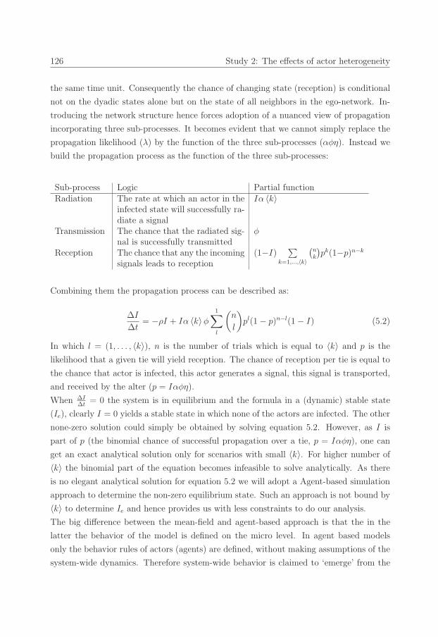
70_Erim_Vermeer Stand.job
126 Study 2: The effects of actor heterogeneity
the same time unit. Consequently the chance of changing state (reception) is conditional
not on the dyadic states alone but on the state of all neighbors in the ego-network. In-
troducing the network structure hence forces adoption of a nuanced view of propagation
incorporating three sub-processes. It becomes evident that we cannot simply replace the
propagation likelihood (λ) by the function of the three sub-processes (αφη). Instead we
build the propagation process as the function of the three sub-processes:
Sub-process Logic Partial functionRadiation The rate at which an actor in the
infected state will successfully ra-diate a signal
Iα 〈k〉
Transmission The chance that the radiated sig-nal is successfully transmitted
φ
Reception The chance that any the incomingsignals leads to reception
(1−I)∑
k=1,...,〈k〉
(nk
)pk(1−p)n−k
Combining them the propagation process can be described as:
ΔI
Δt= −ρI + Iα 〈k〉φ
1∑l
(n
l
)pl(1− p)n−l(1− I) (5.2)
In which l = (1, . . . , 〈k〉), n is the number of trials which is equal to 〈k〉 and p is the
likelihood that a given tie will yield reception. The chance of reception per tie is equal to
the chance that actor is infected, this actor generates a signal, this signal is transported,
and received by the alter (p = Iαφη).
When ΔIΔt
= 0 the system is in equilibrium and the formula in a (dynamic) stable state
(Ie), clearly I = 0 yields a stable state in which none of the actors are infected. The other
none-zero solution could simply be obtained by solving equation 5.2. However, as I is
part of p (the binomial chance of successful propagation over a tie, p = Iαφη), one can
get an exact analytical solution only for scenarios with small 〈k〉. For higher number of
〈k〉 the binomial part of the equation becomes infeasible to solve analytically. As there
is no elegant analytical solution for equation 5.2 we will adopt a Agent-based simulation
approach to determine the non-zero equilibrium state. Such an approach is not bound by
〈k〉 to determine Ie and hence provides us with less constraints to do our analysis.
The big difference between the mean-field and agent-based approach is that the in the
latter the behavior of the model is defined on the micro level. In agent based models
only the behavior rules of actors (agents) are defined, without making assumptions of the
system-wide dynamics. Therefore system-wide behavior is claimed to ‘emerge’ from the
71_Erim_Vermeer Stand.job
5.3 Simulation 127
micro-level interactions rather than being predefined in the model. Additional benefit
of this type of method is that as behavior is defined on the actor level (rather than the
system level) it allows for easily incorporating heterogeneity in actor behavior.
5.2.5 Heterogeneity of actor behavior
We include the notion of actor heterogeneity into our model by assuming that each actor
has a (latent) vector of characteristics c which determines its propensity to send out
(radiate) and respond to (receive) propagation signals; c can vary for each actor and over
time and thus ci,t describes the characteristics of actor i on time t. In order to focus
on heterogeneity in space rather than time we will assume that the characteristics are
stable over time (ci,t = ci,t+1). As we assume that actor characteristics influence the
local propagation mechanism, including the actor heterogeneity requires replacing the
global radiation and reception parameters (α, η) with local parameters per actor αi,e and
ηe,i respectively. For simplicity we will assume that actors do have a preference for ties
during radiation and reception ((αi,1 = αi,2... = αi,e = αi) and (ηi,1 = ηi,2... = ηi,e =
ηi)), resulting in a vector A (A = (α1, ..., αi)) capturing radiation probabilities and a
vector Ψ (Ψ = (η1, ..., ηi)) capturing reception probabilities. When comparing different
propagation processes we pose that the average radiation (and reception) remains equal
in all (x) settings (α = A1 = Ax and η = Ψ1 = Ψx). Having a model with local
propagation parameters, we now can introduce heterogeneity into the system by assuming
heterogeneity in the characteristics (ci) of part population, as this would yield only a
change in an individual’s radiation and/or reception probabilities we can also simply
change these parameters directly. Consequently, we start from the simplest scenario
of heterogeneity in which we create two groups of actors, each with different radiation
(reception (or both)) and compare the propagation outcomes to those of the unperturbed
(default) scenario.
5.3 Simulation
We explore the influence of actor heterogeneity and the consequent heterogeneity in prop-
agation mechanism by means of Agent-based simulation. As input for this simulation
we generate a fixed regular network structure with N actors, on which we will let a
propagation process run from a single seed. We let this process run until it reaches the
approximate dynamic equilibrium, at which point we can determine the prevalence of
the process and the time it took to reach this (semi) stable state. As results of a single

71_Erim_Vermeer Stand.job
128 Study 2: The effects of actor heterogeneity
simulation run would be very susceptible for variations due to stochasticity we increase
the robustness of our results by bootstrapping each simulation N times. The results are
averaged over this bootstrapped sample, any simulation which converges into the stable
state in which the propagation process dies out (Ie = 0) will be ignored. As using a
simulation approach requires fixing some of the parameters at arbitrary values, the next
section will address the parametrization of the simulation in more detail.
5.3.1 Parametrization of the simulation setting
First the simulation requires a network structure on which the process can propagate.
We generate a regular three-dimensional lattice network, in which each actor is connected
to its two nearest neighbors on each dimension. We assume the network is wrapped and
hence that each dimension is circular, consequently each actor has a degree of 6, and the
lattice has no boundaries and is fully regular. Each dimension has 10 actors resulting in
a total population of 1.000 actors (N = 1.000).
Second we fix arbitrary values for the propagation process. The default scenario assumes
all three sub-processes play an equally strong role in propagation (α = φ = η = 0.5),
resulting in an overall propagation likelihood (λ) equal to 0.125 (0.5× 0.5× 0.5). The re-
covery likelihood is fixed at an arbitrary value (ρ = 0.2) such that the epidemic threshold
is surpassed and widespread propagation is to be expected.
Third an arbitrary amount of heterogeneity has to be introduced into the actor behavior.
We select a group of arbitrary size g, and hence divide the population into two groups
of size g and 1 − g respectively. In our default scenario g = (13N) and hence group 1
holds 13(g1 = 1
3N) and group 2 holds 2
3of the population (g2 = 2
3N). Actors are ran-
domly assigned to either one of these groups. For the first group we adjust the radiation
and/or reception likelihood with an arbitrary amount β. We will refer to this adjustment
to group 1 as a ‘perturbation’, which will effectively will mean a reduction of the given
likelihood by β. This effectively means that positive values of β decrease the likelihood of
radiation (and/or reception) in group 1. As we want to keep the average radiation (and
reception) equal in the population any perturbation in group 1 need to be compensated
by changing the radiation (and/or reception) of the second group as well. We spread this
second change equally among the members of the second group and therefore their radi-
ation (or reception) will change with a factor β g2g1
(which is 0.5β in the default scenario).
Consequently the perturbation creates two groups in which actors have different local
propagation dynamics (based on latent actor characteristics), representing the simplest
case of heterogeneity of actors.

72_Erim_Vermeer Stand.job
5.3 Simulation 129
5.3.2 Simulation results heterogeneity
The analysis of the effects of heterogeneity actor behavior will consist of three sets of
simulations; each focusing on a different type of perturbation. The first set will consider
varying perturbation sizes (β) to the radiation sub-process, the second set of simulations
will apply the same perturbations to the reception sub-process, and the third set will
apply perturbations to both the radiation and reception at the same time.
5.3.2.1 Heterogeneity in radiation
The results of the first set of simulations can be found in figure 5.1, and show the ef-
fects of perturbing the radiation with different strengths (β). These results reveal that
heterogeneity in the radiation process (regardless of its size) yields no significantly differ-
ent prevalence for the propagation process. Based on these findings we could state that
the prevalence seems unaffected by heterogeneity in the radiation process. Remarkably
these results also do indicate that for the extreme perturbations in heterogeneity (β =
respectively −0.5,−0.45, 0.5 or 0.45) the amount time it takes to reach equilibrium (Ie)
is larger, and hence the propagation process seems to be slower.
0 20 40 60 80 100
0.0
0.2
0.4
0.6
0.8
1.0
Time
prev
alen
ce
● ● ● ● ● ● ● ● ●●
●●
●
●
●
●
●
●
●
●
●
●
●
●
●
●
●
●
●
●
●
●
●
●
●
●●
●● ● ● ● ● ● ● ● ● ● ● ● ● ● ● ● ● ● ● ● ● ● ● ● ● ● ● ● ● ● ● ● ● ● ● ● ● ● ● ● ● ● ● ● ● ● ● ● ● ● ● ● ● ● ● ● ● ● ● ● ● ●
● ● ● ● ● ● ● ● ● ●●
●●
●●
●
●
●
●
●
●
●
●
●
●
●
●
●
●
●
●
●
●
●●
●●
● ● ● ● ● ● ● ● ● ● ● ● ● ● ● ● ● ● ● ● ● ● ● ● ● ● ● ● ● ● ● ● ● ● ● ● ● ● ● ● ● ● ● ● ● ● ● ● ● ● ● ● ● ● ● ● ● ● ● ● ● ● ●
●
●
Default Scenarioβ= −0.1β= −0.2β= −0.3β= −0.4β= −0.45β= −0.5
(a) The prevalence under negative reductions,increasing the radiation the targeted group(1)by β
0 20 40 60 80 100
0.0
0.2
0.4
0.6
0.8
1.0
Time
prev
alen
ce
● ● ● ● ● ● ● ● ●●
●●
●
●
●
●
●
●
●
●
●
●
●
●
●
●
●
●
●
●
●
●
●
●
●
●●
●● ● ● ● ● ● ● ● ● ● ● ● ● ● ● ● ● ● ● ● ● ● ● ● ● ● ● ● ● ● ● ● ● ● ● ● ● ● ● ● ● ● ● ● ● ● ● ● ● ● ● ● ● ● ● ● ● ● ● ● ● ●
● ● ● ● ● ● ● ● ● ● ●●
●●
●●
●
●
●
●
●
●
●
●
●
●
●
●
●
●
●
●
●
●●
●●
● ● ● ● ● ● ● ● ● ● ● ● ● ● ● ● ● ● ● ● ● ● ● ● ● ● ● ● ● ● ● ● ● ● ● ● ● ● ● ● ● ● ● ● ● ● ● ● ● ● ● ● ● ● ● ● ● ● ● ● ● ● ●
●
●
Default Scenarioβ= 0.1β= 0.2β= 0.3β= 0.4β= 0.45β= 0.5
(b) The prevalence under positive reductions,lowering the radiation of the targeted group(1)by β
Figure 5.1: The prevalence under different perturbations of the radiation sub-process
Especially when looking at figure 5.2, which depicts the rate at which prevalence changes
over time, one can see that the peak of the speed of propagation is reduced when het-
erogeneity in the radiation is introduced. Suggesting that the maximum rate at which
the population becomes infected is lower when there is heterogeneity in the radiation of
actors. Furthermore one can note that the reduction in height of the peak is offset by
extending the width of the peak, suggesting that scenarios with more heterogeneity in
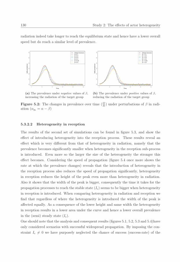
72_Erim_Vermeer Stand.job
130 Study 2: The effects of actor heterogeneity
radiation indeed take longer to reach the equilibrium state and hence have a lower overall
speed but do reach a similar level of prevalence.
0 20 40 60 80 100
0.00
0.01
0.02
0.03
0.04
0.05
0.06
Time
delta
pre
vale
nce
● ●●
●●
●●
●
●
●
●
●
●
●
●
●
●
●
●
●
●
●
●
●
● ●
●
●
●
●
●
●
●
●
●
●
●
●●
●
● ●
● ●●
●
● ●
●
●
●●
●
●
●
●●
●
●●
●
● ●
●
●
●●
●●
●
● ●
●
●
●●
●●
● ● ●●
●
●
● ●● ● ● ● ●
●
●●
● ●●
●
●●● ● ●
●●
●●
●
●
●
●
●
●
●
●
●
●
●
●
●
●
● ●● ●
●
●
●
●
●
●
●
●
●
●
●
●●
●●
●●
● ● ●●
● ●● ●
●●
●
●●
●
● ●
●
●
●●
● ●
●●
●
●●
● ● ●●
●
●
● ●● ●
● ● ●●
●
● ●●
●● ● ●
●●
●
●
● ●●
●
●
Default Scenarioβ= 0.1β= 0.2β= 0.3β= 0.4β= 0.45β= 0.5
(a) The prevalence under negative values of β,increasing the radiation of the target group
0 20 40 60 80 100
0.00
0.01
0.02
0.03
0.04
0.05
0.06
Time
delta
pre
vale
nce
● ●●
●●
●●
●
●
●
●
●
●
●
●
●
●
●
●
●
●
●
●
●
● ●
●
●
●
●
●
●
●
●
●
●
●
●●
●
● ●
● ●●
●
● ●
●
●
●●
●
●
●
●●
●
●●
●
● ●
●
●
●●
●●
●
● ●
●
●
●●
●●
● ● ●●
●
●
● ●● ● ● ● ●
●
●●
● ●●
●
●● ● ● ● ●●
●●
●
●●
●
●
●
●
●
●
●
●
●
●
●
●
● ●
●
●
●
●
●
●
●
●
●
●
●
●
●●
●
●● ●
●●
●
● ●
●●
●
●
●
●● ● ● ●
●● ●
●● ● ● ● ● ●
●
● ●
● ● ● ●● ● ●
●●
● ● ● ● ●● ● ●
●●
●●
●●
●
●●
●●
●
●
Default Scenarioβ= −0.1β= −0.2β= −0.3β= −0.4β= −0.45β= −0.5
(b) The prevalence under positive values of β,reducing the radiation of the target group
Figure 5.2: The changes in prevalence over time ( δIδt) under perturbations of β in radi-
ation (αg1 = α− β)
5.3.2.2 Heterogeneity in reception
The results of the second set of simulations can be found in figure 5.3, and show the
effect of introducing heterogeneity into the reception process. These results reveal an
effect which is very different from that of heterogeneity in radiation, namely that the
prevalence becomes significantly smaller when heterogeneity in the reception sub-process
is introduced. Even more so the larger the size of the heterogeneity the stronger this
effect becomes. Considering the speed of propagation (figure 5.4 once more shows the
rate at which the prevalence changes) reveals that the introduction of heterogeneity in
the reception process also reduces the speed of propagation significantly, heterogeneity
in reception reduces the height of the peak even more than heterogeneity in radiation.
Also it shows that the width of the peak is bigger, consequently the time it takes for the
propagation processes to reach the stable state (Ie) seems to be bigger when heterogeneity
in reception is introduced. When comparing heterogeneity in radiation and reception we
find that regardless of where the heterogeneity is introduced the width of the peak is
affected equally. As a consequence of the lower height and same width the heterogeneity
in reception results in a lower area under the curve and hence a lower overall prevalence
in the (semi) steady state (Ie).
One should note that the analysis and consequent results (figures 5.1, 5.2, 5.3 and 5.4)have
only considered scenarios with successful widespread propagation. By imposing the con-
straint Ie �= 0 we have purposely neglected the chance of success (success-rate) of the
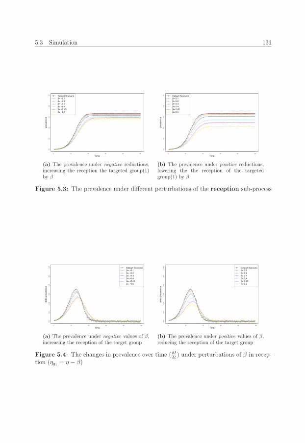
73_Erim_Vermeer Stand.job
5.3 Simulation 131
0 20 40 60 80 100
0.0
0.2
0.4
0.6
0.8
1.0
Time
prev
alen
ce
● ● ● ● ● ● ● ● ●●
●●
●
●
●
●
●
●
●
●
●
●
●
●
●
●
●
●
●
●
●
●
●
●
●
●●
●● ● ● ● ● ● ● ● ● ● ● ● ● ● ● ● ● ● ● ● ● ● ● ● ● ● ● ● ● ● ● ● ● ● ● ● ● ● ● ● ● ● ● ● ● ● ● ● ● ● ● ● ● ● ● ● ● ● ● ● ● ●
● ● ● ● ● ● ● ● ● ●●
●●
●●
●
●
●
●
●
●
●
●
●
●
●
●
●
●
●
●
●
●
●●
●●
●● ● ● ● ● ● ● ● ● ● ● ● ● ● ● ● ● ● ● ● ● ● ● ● ● ● ● ● ● ● ● ● ● ● ● ● ● ● ● ● ● ● ● ● ● ● ● ● ● ● ● ● ● ● ● ● ● ● ● ● ● ●
●
●
Default Scenarioβ= −0.1β= −0.2β= −0.3β= −0.4β= −0.45β= −0.5
(a) The prevalence under negative reductions,increasing the reception the targeted group(1)by β
0 20 40 60 80 100
0.0
0.2
0.4
0.6
0.8
1.0
Time
prev
alen
ce
● ● ● ● ● ● ● ● ●●
●●
●
●
●
●
●
●
●
●
●
●
●
●
●
●
●
●
●
●
●
●
●
●
●
●●
●● ● ● ● ● ● ● ● ● ● ● ● ● ● ● ● ● ● ● ● ● ● ● ● ● ● ● ● ● ● ● ● ● ● ● ● ● ● ● ● ● ● ● ● ● ● ● ● ● ● ● ● ● ● ● ● ● ● ● ● ● ●
● ● ● ● ● ● ● ● ● ●●
●●
●●
●
●
●
●
●
●
●
●
●
●
●
●
●
●
●
●
●
●
●●
●●
● ● ● ● ● ● ● ● ● ● ● ● ● ● ● ● ● ● ● ● ● ● ● ● ● ● ● ● ● ● ● ● ● ● ● ● ● ● ● ● ● ● ● ● ● ● ● ● ● ● ● ● ● ● ● ● ● ● ● ● ● ● ●
●
●
Default Scenarioβ= 0.1β= 0.2β= 0.3β= 0.4β= 0.45β= 0.5
(b) The prevalence under positive reductions,lowering the the reception of the targetedgroup(1) by β
Figure 5.3: The prevalence under different perturbations of the reception sub-process
0 20 40 60 80 100
0.00
0.01
0.02
0.03
0.04
0.05
0.06
Time
delta
pre
vale
nce
● ●●
●●
●●
●
●
●
●
●
●
●
●
●
●
●
●
●
●
●
●
●
● ●
●
●
●
●
●
●
●
●
●
●
●
●●
●
● ●
● ●●
●
● ●
●
●
●●
●
●
●
●●
●
●●
●
● ●
●
●
●●
●●
●
● ●
●
●
●●
●●
● ● ●●
●
●
● ●● ● ● ● ●
●
●●
● ●●
●
●● ● ● ●●
●●
●
●●
●
●
●
●
●
●
●
●
●
●
●
●
●
● ●●
●
●
●
●
●
●
●
●
●
●●
●
●
● ●
●
●
●● ● ● ●
●
● ●● ●
●
●
●
● ●● ● ●
●
●●
● ● ● ● ●●
●● ●
●●
●●
●●
●
●●
●
●●
●●
●
● ●
●● ●
● ●●
●
● ●
●
●
Default Scenarioβ= −0.1β= −0.2β= −0.3β= −0.4β= −0.45β= −0.5
(a) The prevalence under negative values of β,increasing the reception of the target group
0 20 40 60 80 100
0.00
0.01
0.02
0.03
0.04
0.05
0.06
Time
delta
pre
vale
nce
● ●●
●●
●●
●
●
●
●
●
●
●
●
●
●
●
●
●
●
●
●
●
● ●
●
●
●
●
●
●
●
●
●
●
●
●●
●
● ●
● ●●
●
● ●
●
●
●●
●
●
●
●●
●
●●
●
● ●
●
●
●●
●●
●
● ●
●
●
●●
●●
● ● ●●
●
●
● ●● ● ● ● ●
●
●●
● ●●
●
●● ● ●●
●●
●●
●
●
●
●
●
●
●
●
●
●
●
●
●
●
●
●
●●
● ●
●
●
●
●
●
●
●
●
●●
●
● ●●
● ●●
● ● ●●
●
●● ●
●
●●
●●
● ●
●
● ●
●●
●●
●●
● ● ●
●● ● ●
●
●● ● ● ●
●
●
●● ●
●
●
●● ● ● ● ●
●●
● ●
●
●
Default Scenarioβ= 0.1β= 0.2β= 0.3β= 0.4β= 0.45β= 0.5
(b) The prevalence under positive values of β,reducing the reception of the target group
Figure 5.4: The changes in prevalence over time ( δIδt) under perturbations of β in recep-
tion (ηg1 = η − β)
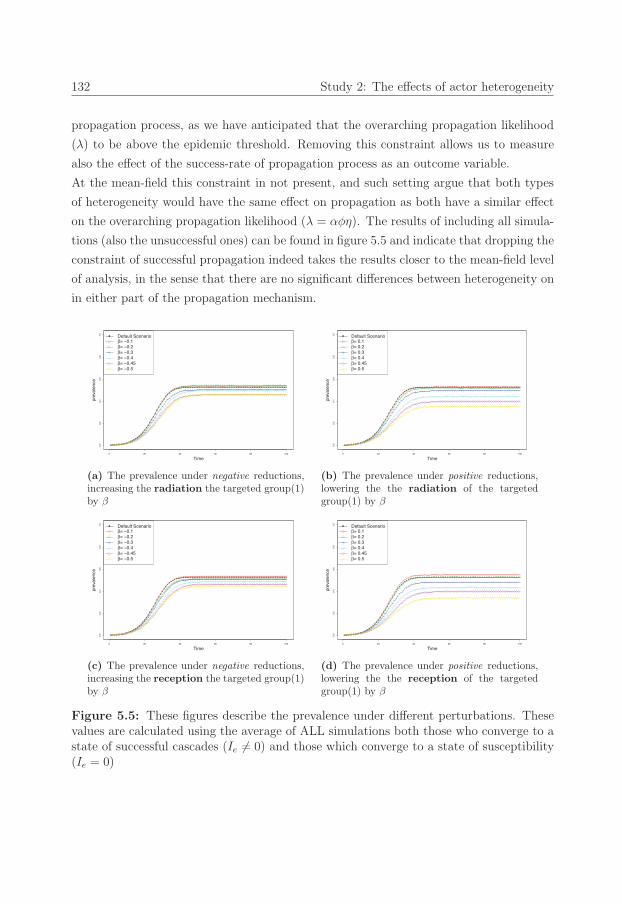
73_Erim_Vermeer Stand.job
132 Study 2: The effects of actor heterogeneity
propagation process, as we have anticipated that the overarching propagation likelihood
(λ) to be above the epidemic threshold. Removing this constraint allows us to measure
also the effect of the success-rate of propagation process as an outcome variable.
At the mean-field this constraint in not present, and such setting argue that both types
of heterogeneity would have the same effect on propagation as both have a similar effect
on the overarching propagation likelihood (λ = αφη). The results of including all simula-
tions (also the unsuccessful ones) can be found in figure 5.5 and indicate that dropping the
constraint of successful propagation indeed takes the results closer to the mean-field level
of analysis, in the sense that there are no significant differences between heterogeneity on
in either part of the propagation mechanism.
0 20 40 60 80 100
0.0
0.2
0.4
0.6
0.8
1.0
Time
prev
alen
ce
● ● ● ● ● ● ● ● ● ●●
●●
●●
●
●
●
●
●
●
●
●
●
●
●
●
●
●
●
●
●
●
●
●●
●● ● ● ● ● ● ● ● ● ● ● ● ● ● ● ● ● ● ● ● ● ● ● ● ● ● ● ● ● ● ● ● ● ● ● ● ● ● ● ● ● ● ● ● ● ● ● ● ● ● ● ● ● ● ● ● ● ● ● ● ● ● ●
● ● ● ● ● ● ● ● ● ● ● ●●
●●
●●
●
●
●
●
●
●
●
●
●
●
●
●
●
●
●
●●
●●
● ● ● ● ● ● ● ● ● ● ● ● ● ● ● ● ● ● ● ● ● ● ● ● ● ● ● ● ● ● ● ● ● ● ● ● ● ● ● ● ● ● ● ● ● ● ● ● ● ● ● ● ● ● ● ● ● ● ● ● ● ● ● ●
●
●
Default Scenarioβ= −0.1β= −0.2β= −0.3β= −0.4β= −0.45β= −0.5
(a) The prevalence under negative reductions,increasing the radiation the targeted group(1)by β
0 20 40 60 80 100
0.0
0.2
0.4
0.6
0.8
1.0
Time
prev
alen
ce
● ● ● ● ● ● ● ● ● ●●
●●
●●
●
●
●
●
●
●
●
●
●
●
●
●
●
●
●
●
●
●
●
●●
●● ● ● ● ● ● ● ● ● ● ● ● ● ● ● ● ● ● ● ● ● ● ● ● ● ● ● ● ● ● ● ● ● ● ● ● ● ● ● ● ● ● ● ● ● ● ● ● ● ● ● ● ● ● ● ● ● ● ● ● ● ● ●
● ● ● ● ● ● ● ● ● ● ● ●●
●●
●●
●
●
●
●
●
●
●
●
●
●
●
●
●
●
●
●●
●●
● ● ● ● ● ● ● ● ● ● ● ● ● ● ● ● ● ● ● ● ● ● ● ● ● ● ● ● ● ● ● ● ● ● ● ● ● ● ● ● ● ● ● ● ● ● ● ● ● ● ● ● ● ● ● ● ● ● ● ● ● ● ● ●
●
●
Default Scenarioβ= 0.1β= 0.2β= 0.3β= 0.4β= 0.45β= 0.5
(b) The prevalence under positive reductions,lowering the the radiation of the targetedgroup(1) by β
0 20 40 60 80 100
0.0
0.2
0.4
0.6
0.8
1.0
Time
prev
alen
ce
● ● ● ● ● ● ● ● ● ●●
●●
●●
●
●
●
●
●
●
●
●
●
●
●
●
●
●
●
●
●
●
●
●●
●● ● ● ● ● ● ● ● ● ● ● ● ● ● ● ● ● ● ● ● ● ● ● ● ● ● ● ● ● ● ● ● ● ● ● ● ● ● ● ● ● ● ● ● ● ● ● ● ● ● ● ● ● ● ● ● ● ● ● ● ● ● ●
● ● ● ● ● ● ● ● ● ● ● ●●
●●
●●
●
●
●
●
●
●
●
●
●
●
●
●
●
●
●
●●
●●
●● ● ● ● ● ● ● ● ● ● ● ● ● ● ● ● ● ● ● ● ● ● ● ● ● ● ● ● ● ● ● ● ● ● ● ● ● ● ● ● ● ● ● ● ● ● ● ● ● ● ● ● ● ● ● ● ● ● ● ● ● ● ●
●
●
Default Scenarioβ= −0.1β= −0.2β= −0.3β= −0.4β= −0.45β= −0.5
(c) The prevalence under negative reductions,increasing the reception the targeted group(1)by β
0 20 40 60 80 100
0.0
0.2
0.4
0.6
0.8
1.0
Time
prev
alen
ce
● ● ● ● ● ● ● ● ● ●●
●●
●●
●
●
●
●
●
●
●
●
●
●
●
●
●
●
●
●
●
●
●
●●
●● ● ● ● ● ● ● ● ● ● ● ● ● ● ● ● ● ● ● ● ● ● ● ● ● ● ● ● ● ● ● ● ● ● ● ● ● ● ● ● ● ● ● ● ● ● ● ● ● ● ● ● ● ● ● ● ● ● ● ● ● ● ●
● ● ● ● ● ● ● ● ● ● ●●
●●
●●
●●
●
●
●
●
●
●
●
●
●
●
●
●
●
●
●●
●●
● ● ● ● ● ● ● ● ● ● ● ● ● ● ● ● ● ● ● ● ● ● ● ● ● ● ● ● ● ● ● ● ● ● ● ● ● ● ● ● ● ● ● ● ● ● ● ● ● ● ● ● ● ● ● ● ● ● ● ● ● ● ● ●
●
●
Default Scenarioβ= 0.1β= 0.2β= 0.3β= 0.4β= 0.45β= 0.5
(d) The prevalence under positive reductions,lowering the the reception of the targetedgroup(1) by β
Figure 5.5: These figures describe the prevalence under different perturbations. Thesevalues are calculated using the average of ALL simulations both those who converge to astate of successful cascades (Ie �= 0) and those which converge to a state of susceptibility(Ie = 0)
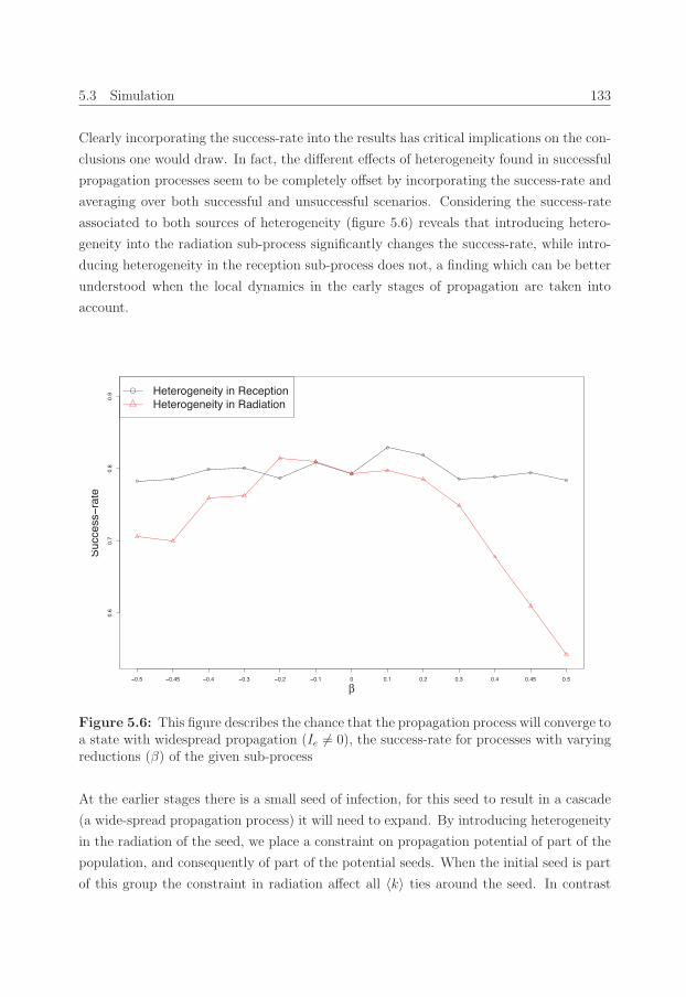
74_Erim_Vermeer Stand.job
5.3 Simulation 133
Clearly incorporating the success-rate into the results has critical implications on the con-
clusions one would draw. In fact, the different effects of heterogeneity found in successful
propagation processes seem to be completely offset by incorporating the success-rate and
averaging over both successful and unsuccessful scenarios. Considering the success-rate
associated to both sources of heterogeneity (figure 5.6) reveals that introducing hetero-
geneity into the radiation sub-process significantly changes the success-rate, while intro-
ducing heterogeneity in the reception sub-process does not, a finding which can be better
understood when the local dynamics in the early stages of propagation are taken into
account.
β
Suc
cess−
rate
●●
● ●
●
●
●
●
●
●●
●
●
−0.5 −0.45 −0.4 −0.3 −0.2 −0.1 0 0.1 0.2 0.3 0.4 0.45 0.5
0.6
0.7
0.8
0.9 ● Heterogeneity in Reception
Heterogeneity in Radiation
Figure 5.6: This figure describes the chance that the propagation process will converge toa state with widespread propagation (Ie �= 0), the success-rate for processes with varyingreductions (β) of the given sub-process
At the earlier stages there is a small seed of infection, for this seed to result in a cascade
(a wide-spread propagation process) it will need to expand. By introducing heterogeneity
in the radiation of the seed, we place a constraint on propagation potential of part of the
population, and consequently of part of the potential seeds. When the initial seed is part
of this group the constraint in radiation affect all 〈k〉 ties around the seed. In contrast
74_Erim_Vermeer Stand.job
134 Study 2: The effects of actor heterogeneity
a constraint in reception would only apply to those ties which are directed towards the
constrained alters, and hence will only affect the propagation likelihood of part of the
ties. Consequently the constraint put into place by heterogeneity in radiation is clearly
strongest in the early stages of the process where there is a low number of seeds. Even
more so the stochastic nature of recovery in the model implies that in the early stages
the propagation process runs the bigger risk of ending up in the stable state without
infected actors, simply due to the limited set of seeds. Therefore in our model introducing
heterogeneity increases the risk of going extinct in the early stages, and as the constraint
for heterogeneity in radiation is stronger we see the biggest effect on the success-rate in
those scenarios.
In contrast in the later stages of propagation,where the prevalence is measured, susceptible
actors are prone to be subject to a multitude of signals. Here the constraint in radiation
would only affect the likelihood of propagation over some of the incoming ties (only
those ties coming from low radiation actors) whereas a constraint in reception would
affect the likelihood of propagation over all 〈k〉 ties surrounding the to-be infected actor.
Consequently the heterogeneity in reception hampers the overall prevalence more than a
similar heterogeneity in radiation, a finding which is indeed supported by figures 5.1 and
5.3.
In conclusion, based on the first two sets of simulations we therefore argue that on average
the result of introduction heterogeneity in either radiation or reception seem to be similar,
both seem to reduce the prevalence of propagation, while the mechanisms by which they
achieve this goal differ radically. Where heterogeneity in radiation reduces mainly the
chances of widespread propagation (the success-rate), heterogeneity in reception reduces
mainly the prevalence of successful propagation.
5.3.2.3 Combining heterogeneity in radiation and reception
In the previous section we have studied the effects of heterogeneity in either radiation or
reception. However, building on the notion that there is a set of latent actor characteris-
tics that drive heterogeneity in the radiation and reception of actors, it seem more likely
to assume that both effects occur simultaneously. Therefore, in the next (third) set of
simulations, such scenarios are explored.
Starting from the simplest possible notion one could assume that both radiation as well as
reception are affected equally by the latent actor characteristics. This effectively means
that the group of actors which receives a perturbation in the radiation is also the group
receives the same perturbation in the reception (grad1 = grec1 ). As in this scenario the
membership to the perturbed group (grad1 , grec1 ) is linked this scenario is referred to as the

75_Erim_Vermeer Stand.job
5.3 Simulation 135
linked assignment. The other extreme of the spectrum would be a scenario in which the
membership to the perturbed group for radiation (grad1 ) is independent from the mem-
bership to the perturbed group for reception (grec1 ). In this scenario group membership is
assigned randomly, and hence this scenario is referred to as random assignment. While
many other arbitrary ways could be proposed in which the latent actor characteristics
could affect the local propagation mechanism, in this study we focus on two types of ef-
fects mentioned above; linked assignment and random assignment, as this is the simplest
viable model which captures the interaction between heterogeneity in both parts of the
sub-process.
5.3.2.4 Linked assignment
The linked assignment approach (like the previous simulations) yields two groups of actors.
For the first group both radiation as well as reception are perturbed by reducing them
by β, and for the second group radiation and reception are increased so that the average
radiation and reception remain the same and hence the equality constraint is met. The
results of the linked assignment scenario (Figure 5.7) show that introducing heterogeneity
in radiation and reception at the same time both increases the speed and reduces the
prevalence of the infection.
0 20 40 60 80 100
0.0
0.2
0.4
0.6
0.8
1.0
Time
prev
alen
ce
● ● ● ● ● ● ● ● ●●
●●
●
●
●
●
●
●
●
●
●
●
●
●
●
●
●
●
●
●
●
●
●
●
●
●●
●● ● ● ● ● ● ● ● ● ● ● ● ● ● ● ● ● ● ● ● ● ● ● ● ● ● ● ● ● ● ● ● ● ● ● ● ● ● ● ● ● ● ● ● ● ● ● ● ● ● ● ● ● ● ● ● ● ● ● ● ● ●
● ● ● ● ● ● ● ● ● ●●
●●
●●
●
●
●
●
●
●
●
●
●
●
●
●
●
●
●
●
●
●
●●
●●
● ● ● ● ● ● ● ● ● ● ● ● ● ● ● ● ● ● ● ● ● ● ● ● ● ● ● ● ● ● ● ● ● ● ● ● ● ● ● ● ● ● ● ● ● ● ● ● ● ● ● ● ● ● ● ● ● ● ● ● ● ● ●
●
●
Default Scenarioβ= −0.1β= −0.2β= −0.3β= −0.4β= −0.45β= −0.5
(a) The prevalence under negative values ofperturbation (β < 0) in a setting of linked as-signment to groups, effectively increasing boththe radiation and reception of the targetedgroup (g1) by β
0 20 40 60 80 100
0.0
0.2
0.4
0.6
0.8
1.0
Time
prev
alen
ce
● ● ● ● ● ● ● ● ●●
●●
●
●
●
●
●
●
●
●
●
●
●
●
●
●
●
●
●
●
●
●
●
●
●
●●
●● ● ● ● ● ● ● ● ● ● ● ● ● ● ● ● ● ● ● ● ● ● ● ● ● ● ● ● ● ● ● ● ● ● ● ● ● ● ● ● ● ● ● ● ● ● ● ● ● ● ● ● ● ● ● ● ● ● ● ● ● ●
● ● ● ● ● ● ● ● ● ●●
●●
●●
●
●
●
●
●
●
●
●
●
●
●
●
●
●
●
●
●
●
●●
●●
● ● ● ● ● ● ● ● ● ● ● ● ● ● ● ● ● ● ● ● ● ● ● ● ● ● ● ● ● ● ● ● ● ● ● ● ● ● ● ● ● ● ● ● ● ● ● ● ● ● ● ● ● ● ● ● ● ● ● ● ● ● ●
●
●
Default Scenarioβ= 0.1β= 0.2β= 0.3β= 0.4β= 0.45β= 0.5
(b) The prevalence under positive values of per-turbation (β > 0) in a setting of linked assign-ment to groups, effectively reducing both theradiation and reception of the targeted group(g1) by β
Figure 5.7: The prevalence under different perturbations in the linked assignment sce-nario
While the reduction in prevalence is in line with what one would expect from introduc-
ing heterogeneity, the increased speed seems to be opposite from the previously found
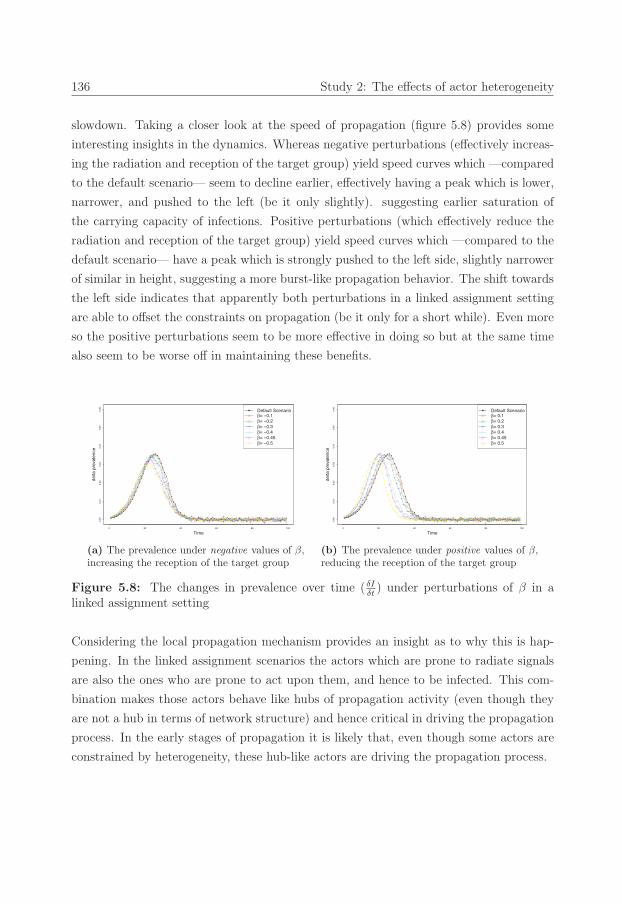
75_Erim_Vermeer Stand.job
136 Study 2: The effects of actor heterogeneity
slowdown. Taking a closer look at the speed of propagation (figure 5.8) provides some
interesting insights in the dynamics. Whereas negative perturbations (effectively increas-
ing the radiation and reception of the target group) yield speed curves which —compared
to the default scenario— seem to decline earlier, effectively having a peak which is lower,
narrower, and pushed to the left (be it only slightly). suggesting earlier saturation of
the carrying capacity of infections. Positive perturbations (which effectively reduce the
radiation and reception of the target group) yield speed curves which —compared to the
default scenario— have a peak which is strongly pushed to the left side, slightly narrower
of similar in height, suggesting a more burst-like propagation behavior. The shift towards
the left side indicates that apparently both perturbations in a linked assignment setting
are able to offset the constraints on propagation (be it only for a short while). Even more
so the positive perturbations seem to be more effective in doing so but at the same time
also seem to be worse off in maintaining these benefits.
0 20 40 60 80 100
0.00
0.01
0.02
0.03
0.04
0.05
0.06
Time
delta
pre
vale
nce
● ●●
●●
●●
●
●
●
●
●
●
●
●
●
●
●
●
●
●
●
●
●
● ●
●
●
●
●
●
●
●
●
●
●
●
●●
●
● ●
● ●●
●
● ●
●
●
●●
●
●
●
●●
●
●●
●
● ●
●
●
●●
●●
●
● ●
●
●
●●
●●
● ● ●●
●
●
● ●● ● ● ● ●
●
●●
● ●●
●
●● ● ● ●●
●●
●
●
●
●
●
●
●
●
●
●
●
●
●
●
●
●● ●
● ●
●
●
●
●
●
●
●
●
●
●
●
● ●
●●
● ●●
●
● ●●
●●
● ● ●
●
●
●
● ●● ●
● ●
●
●●
● ● ● ●●
● ● ● ● ●●
●
● ●● ●
● ●●
●
●
● ● ● ● ●
●
●
● ●
●
●
●
●
●
Default Scenarioβ= −0.1β= −0.2β= −0.3β= −0.4β= −0.45β= −0.5
(a) The prevalence under negative values of β,increasing the reception of the target group
0 20 40 60 80 100
0.00
0.01
0.02
0.03
0.04
0.05
0.06
Time
delta
pre
vale
nce
● ●●
●●
●●
●
●
●
●
●
●
●
●
●
●
●
●
●
●
●
●
●
● ●
●
●
●
●
●
●
●
●
●
●
●
●●
●
● ●
● ●●
●
● ●
●
●
●●
●
●
●
●●
●
●●
●
● ●
●
●
●●
●●
●
● ●
●
●
●●
●●
● ● ●●
●
●
● ●● ● ● ● ●
●
●●
● ●●
●
●● ● ●●
●●
●●
●
●
●
●
●
●
●
●
●
●
●
●
●
●
●●
●●
●
●
●
●
●
●
●
●
●
●
●
●
●●
●●
●● ●
●● ●
● ● ● ●
● ●●
●
●
●● ● ● ●
●● ● ●
●●
●● ● ●
●
●
●● ●
●● ● ●
●
●●
●
● ●● ● ● ●
●
●●
●●
●
●
●
●
●
Default Scenarioβ= 0.1β= 0.2β= 0.3β= 0.4β= 0.45β= 0.5
(b) The prevalence under positive values of β,reducing the reception of the target group
Figure 5.8: The changes in prevalence over time ( δIδt) under perturbations of β in a
linked assignment setting
Considering the local propagation mechanism provides an insight as to why this is hap-
pening. In the linked assignment scenarios the actors which are prone to radiate signals
are also the ones who are prone to act upon them, and hence to be infected. This com-
bination makes those actors behave like hubs of propagation activity (even though they
are not a hub in terms of network structure) and hence critical in driving the propagation
process. In the early stages of propagation it is likely that, even though some actors are
constrained by heterogeneity, these hub-like actors are driving the propagation process.
76_Erim_Vermeer Stand.job
5.3 Simulation 137
We consider two extreme scenarios to clarify these finding. We consider an scenario in
which β = 0.5 and β = −0.5 and provide a numeric example of what is happening during
the early stages of propagation:
• Note that, in the default scenario each infected actor infects approximately 0.75
(kαφη = 6 ∗ 0.5 ∗ 0.5 ∗ 0.5 = 0.75) alters each time unit.
• In the first proposed scenario 13of the population has no radiation and reception
(α − β = 0 and η − β = 0). Consequently, 23of the population has their radiation
and reception increased (to 0.75). In this scenario an infected actor will infect 1.125
(6 ∗ 0.75 ∗ 0.5 ∗ 0.5) alters each time step if it is in group2 (and 0 if the seed is in
group1, in which case the propagation process would die out, and will not be included
in our graph and analysis).
• In the second proposed scenario 13of the actors always radiates and receives (α−β =
1 and η−β = 1). Each infected actor in group1 will thus infect 1.5 alters each time
unit (6 ∗ 1 ∗ 0.5 ∗ 0.5), and each actor in group2 will infect 0.375 alters each time
unit (6 ∗ 0.25 ∗ 0.5 ∗ 0.5). To leverage the the potential speedup it will thus need to
spread towards group1. So while this scenario has the potential to out-perform the
previous one, it will not do so in each scenario, this clearly limits the potential of
reaping the benefits of hub-like actors, and explains why on average it will lag behind
the other scenarios.
What this linked assignment scenario seems to implicate is that the propagation process
can capitalize on a backbone of hub-like actors in the early stages of propagation to offset
the constraints put into place by introducing heterogeneity. These hub-like actors serve
as a ’high-way’ of propagation. But as the size of this highway is limited, once this high-
way becomes saturated the force offsetting the constraints will dissipate and the effects
of heterogeneity start kicking back in.
5.3.2.5 Random assignment
The notion that a set of latent actor characteristics drives both radiation and reception
seems fairly straightforward, the fact that both are affected in the same manner might
be less realistic. Therefore in the following scenario we will relax this assumption by
stating that while the size of the perturbation in radiation and reception remains linked
the actors which receive these perturbation do not need to be. Effectively this means
that the actors which receive a perturbation in radiation are chosen by a process which is
independent of the assignment of the perturbation in reception. As in this scenario there
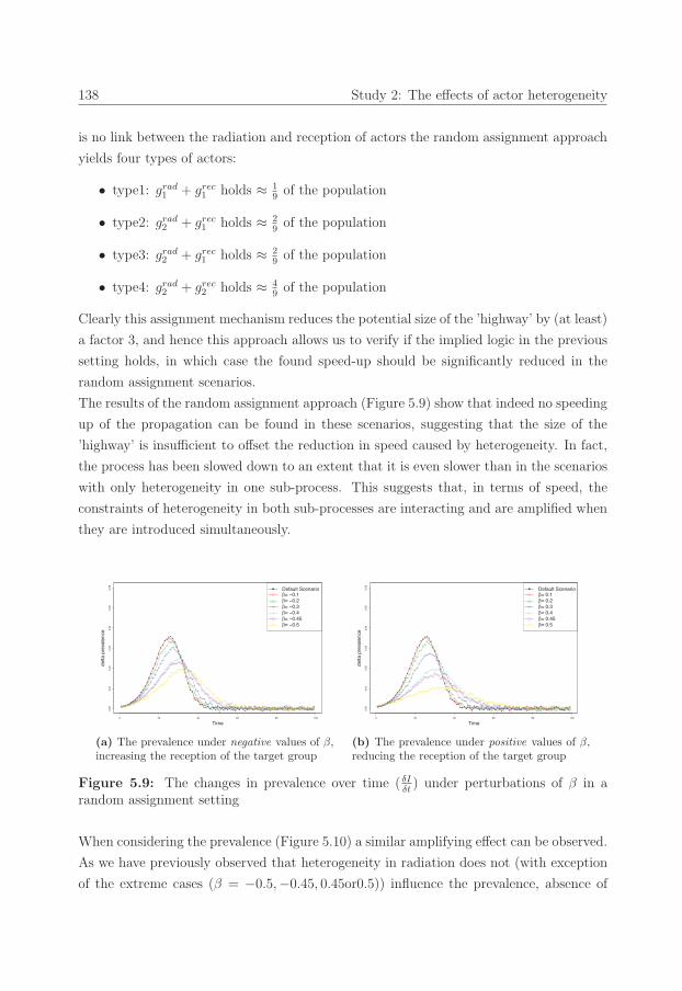
76_Erim_Vermeer Stand.job
138 Study 2: The effects of actor heterogeneity
is no link between the radiation and reception of actors the random assignment approach
yields four types of actors:
• type1: grad1 + grec1 holds ≈ 19of the population
• type2: grad2 + grec1 holds ≈ 29of the population
• type3: grad2 + grec1 holds ≈ 29of the population
• type4: grad2 + grec2 holds ≈ 49of the population
Clearly this assignment mechanism reduces the potential size of the ’highway’ by (at least)
a factor 3, and hence this approach allows us to verify if the implied logic in the previous
setting holds, in which case the found speed-up should be significantly reduced in the
random assignment scenarios.
The results of the random assignment approach (Figure 5.9) show that indeed no speeding
up of the propagation can be found in these scenarios, suggesting that the size of the
’highway’ is insufficient to offset the reduction in speed caused by heterogeneity. In fact,
the process has been slowed down to an extent that it is even slower than in the scenarios
with only heterogeneity in one sub-process. This suggests that, in terms of speed, the
constraints of heterogeneity in both sub-processes are interacting and are amplified when
they are introduced simultaneously.
0 20 40 60 80 100
0.00
0.01
0.02
0.03
0.04
0.05
0.06
Time
delta
pre
vale
nce
● ●●
●●
●●
●
●
●
●
●
●
●
●
●
●
●
●
●
●
●
●
●
● ●
●
●
●
●
●
●
●
●
●
●
●
●●
●
● ●
● ●●
●
● ●
●
●
●●
●
●
●
●●
●
●●
●
● ●
●
●
●●
●●
●
● ●
●
●
●●
●●
● ● ●●
●
●
● ●● ● ● ● ●
●
●●
● ●●
●
●● ● ● ●●
●●
●
●●
●
●
●
●
●
●
●
●
●
●
●
●
●● ● ●
●●
●
●
●
●
●
●
●
●
●
● ●
●
●● ● ●
●● ●
● ● ●
●
● ●●
●●
●●
●
●●
●●
● ● ● ● ●● ●
●
●
●●
● ●● ● ●
● ● ● ●●
●
●
●● ●
●●
●● ● ●
●● ●
●
●
●
Default Scenarioβ= −0.1β= −0.2β= −0.3β= −0.4β= −0.45β= −0.5
(a) The prevalence under negative values of β,increasing the reception of the target group
0 20 40 60 80 100
0.00
0.01
0.02
0.03
0.04
0.05
0.06
Time
delta
pre
vale
nce
● ●●
●●
●●
●
●
●
●
●
●
●
●
●
●
●
●
●
●
●
●
●
● ●
●
●
●
●
●
●
●
●
●
●
●
●●
●
● ●
● ●●
●
● ●
●
●
●●
●
●
●
●●
●
●●
●
● ●
●
●
●●
●●
●
● ●
●
●
●●
●●
● ● ●●
●
●
● ●● ● ● ● ●
●
●●
● ●●
●
●● ● ●●
● ●●
●●
●
●
●
●
●
●
●
●
●
●
●
●
●
●
●● ●
●●
●
●
●
●
●
●
●
●
●
●
●
● ●● ●
●●
● ●●
●
●●
●●
● ●●
●
●●
●●
●● ●
●
●
●
●
●●
● ● ● ●●
●
●●
● ●●
●● ● ● ●
●● ●
●●
●●
● ●● ● ●
●
●
●
Default Scenarioβ= 0.1β= 0.2β= 0.3β= 0.4β= 0.45β= 0.5
(b) The prevalence under positive values of β,reducing the reception of the target group
Figure 5.9: The changes in prevalence over time ( δIδt) under perturbations of β in a
random assignment setting
When considering the prevalence (Figure 5.10) a similar amplifying effect can be observed.
As we have previously observed that heterogeneity in radiation does not (with exception
of the extreme cases (β = −0.5,−0.45, 0.45or0.5)) influence the prevalence, absence of
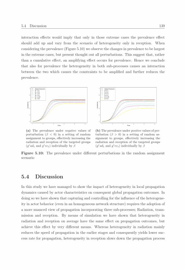
77_Erim_Vermeer Stand.job
5.4 Discussion 139
interaction effects would imply that only in those extreme cases the prevalence effect
should add up and vary from the scenario of heterogeneity only in reception. When
considering the prevalence (Figure 5.10) we observe the changes in prevalence to be largest
in the extreme cases, but present thought out all perturbations. This suggest that, rather
than a cumulative effect, an amplifying effect occurs for prevalence. Hence we conclude
that also for prevalence the heterogeneity in both sub-processes causes an interaction
between the two which causes the constraints to be amplified and further reduces the
prevalence.
0 20 40 60 80 100
0.0
0.2
0.4
0.6
0.8
1.0
Time
prev
alen
ce
● ● ● ● ● ● ● ● ●●
●●
●
●
●
●
●
●
●
●
●
●
●
●
●
●
●
●
●
●
●
●
●
●
●
●●
●● ● ● ● ● ● ● ● ● ● ● ● ● ● ● ● ● ● ● ● ● ● ● ● ● ● ● ● ● ● ● ● ● ● ● ● ● ● ● ● ● ● ● ● ● ● ● ● ● ● ● ● ● ● ● ● ● ● ● ● ● ●
● ● ● ● ● ● ● ● ● ● ●●
●●
●●
●
●
●
●
●
●
●
●
●
●
●
●
●
●
●
●
●
●●
●●
● ● ● ● ● ● ● ● ● ● ● ● ● ● ● ● ● ● ● ● ● ● ● ● ● ● ● ● ● ● ● ● ● ● ● ● ● ● ● ● ● ● ● ● ● ● ● ● ● ● ● ● ● ● ● ● ● ● ● ● ● ● ●
●
●
Default Scenarioβ= −0.1β= −0.2β= −0.3β= −0.4β= −0.45β= −0.5
(a) The prevalence under negative values ofperturbation (β < 0) in a setting of randomassignment to groups, effectively increasing theradiation and reception of the targeted groups(grad1 and grec1) individually by β
0 20 40 60 80 100
0.0
0.2
0.4
0.6
0.8
1.0
Time
prev
alen
ce
● ● ● ● ● ● ● ● ●●
●●
●
●
●
●
●
●
●
●
●
●
●
●
●
●
●
●
●
●
●
●
●
●
●
●●
●● ● ● ● ● ● ● ● ● ● ● ● ● ● ● ● ● ● ● ● ● ● ● ● ● ● ● ● ● ● ● ● ● ● ● ● ● ● ● ● ● ● ● ● ● ● ● ● ● ● ● ● ● ● ● ● ● ● ● ● ● ●
● ● ● ● ● ● ● ● ● ● ●●
●●
●●
●
●
●
●
●
●
●
●
●
●
●
●
●
●
●
●
●
●
●●
●● ● ● ● ● ● ● ● ● ● ● ● ● ● ● ● ● ● ● ● ● ● ● ● ● ● ● ● ● ● ● ● ● ● ● ● ● ● ● ● ● ● ● ● ● ● ● ● ● ● ● ● ● ● ● ● ● ● ● ● ● ● ●
●
●
Default Scenarioβ= 0.1β= 0.2β= 0.3β= 0.4β= 0.45β= 0.5
(b) The prevalence under positive values of per-turbation (β > 0) in a setting of random as-signment to groups, effectively increasing theradiation and reception of the targeted groups(grad1 and grec1) individually by β
Figure 5.10: The prevalence under different perturbations in the random assignmentscenario
5.4 Discussion
In this study we have managed to show the impact of heterogeneity in local propagation
dynamics caused by actor characteristics on consequent global propagation outcomes. In
doing so we have shown that capturing and controlling for the influence of the heterogene-
ity in actor behavior (even in an homogeneous network structure) requires the adoption of
a more nuanced view of propagation incorporating three sub-processes; Radiation, trans-
mission and reception. By means of simulation we have shown that heterogeneity in
radiation and reception on average have the same effect on propagation outcomes, but
achieve this effect by very different means. Whereas heterogeneity in radiation mainly
reduces the speed of propagation in the earlier stages and consequently yields lower suc-
cess rate for propagation, heterogeneity in reception slows down the propagation process
77_Erim_Vermeer Stand.job
140 Study 2: The effects of actor heterogeneity
more in the later stages and consequently reduces the prevalence of the process.
We found that incorporating heterogeneity in both locations in the process (both in radi-
ation and reception) yields an interaction which amplifies the effects of both. This means
that the constraints in both are amplified, but also that for some actors an amplified
positive effect can occur. These actors will becomes more susceptible to propagation and
also will send out more signals. The positive interactions yields a type of actor which
serves as a hub for propagation dynamics, even though it is not a hub in terms of network
structure. Having a substantial amount of these hub-like actors in the network allows
for temporary outperforming the benchmark of a process (which does not include any
heterogeneity). Consequently heterogeneity in local dynamics while generally hampering
propagation can also enable quick ramp-up of the propagation towards a global cascade.
Our finding have some interesting implications policy makers, especially those who intend
to initiate a global cascade (or prevent this). Take for example a marketing setting, and
apply our findings. We have shown that in order to ’create’ a cascade the radiation pro-
cess is critical to take under consideration. Targeting the best radiators will increase the
success rate of such a propagation process and hence are the most useful targets for seed-
ing a product. While this might be logical from a conceptual standpoint this does imply
that no longer the intended users (which are usually those which are most prone to adopt
and hence are characterized by high reception) are to be targeted, instead one should rely
on the fact that these actors will be reached via the propagation process. Similarly in
a setting of contagious disease (where one intents to prevent spreading) assuming a new
infection with very little seeds, one should focus their efforts on those who are likely to
radiate, rather than those who are likely to receive. Clearly the underlying assumption
here is that the cascade can still be averted and pushing the process towards the zero
infection stable (Ie = 0) state is an option, something which is strongly dependent on the
overall contagiousness of the disease.
Furthermore while we find that both locations of heterogeneity (in radiation and recep-
tion) yield on average a similar effect on prevalence, the differences in dynamics of reaching
those have a strong implication for propagation processes that occur in our environment.
As commonly we see cascades occurring only when they have a sufficiently large size, they
are likely to have already passed the survival phase and consequently any influence of het-
erogeneity in radiation seems to have already been accounted for by the time we observe
them. Therefore a fruitful direction for future research would be to see what happens to
our findings when we assume a small group of seeds (rather then a single one).
78_Erim_Vermeer Stand.job
5.4 Discussion 141
Similarly we useful extension of this research would capture the effects of homophily.
While the notion of homophily is touched upon in the literature section of this article it
is not incorporated into the actual model. Given that we have identified the implications
of the highway or backbone of the propagation process, we assume that homophily can
strongly influence the effectiveness of such a feature. Using the analogy of a highway, if
this highway cannot be used to reach the regions of the population far away from the seed
of infection (something which would be in line with the logic of homophily, arguing that
similar actors are clustered) would strongly hamper the benefits of having such a highway.
Of course a competing argument could also be made, a highway can only be effectively
leveraged if they are sufficiently connected, making incorporating the notion of homophily
a logical next step in understanding the effects of heterogeneity in local dynamics.
In conclusion, an interesting observation (which is somewhat outside the scope of our
study) is that while we found that having hub-like actors will facilitate propagation in
the early stages of the propagation process, at some point the inherent constraints of
having hub-like actors (namely that others have their radiation and reception reduced)
do catch up with them. The benchmark will therefore always yield a higher prevalence
in the equilibrium state. The finding that the default scenario (without heterogeneity)
is never surpassed in terms of prevalence indicates that not incorporating heterogeneity
in the modeling of propagation structurally provides an upper bound to the outcomes of
propagation processes, a finding which is in line with the findings of Aral et al. (2013).
This indicates that capturing heterogeneity in our models of propagation facilitates more
depth and detail in the process, but also introduces additional abortive capacity to the
system and reduces the prevalence of infections on them.
In contrast, heterogeneous actor behavior might also be the thing which allows processes
to become a cascade in the first place. A propagation process without average behavior
which allows them to become a system-wide cascade, might be able to leverage a highway
of propagation (facilitated by heterogeneous actor behavior) and consequently cascade
throughout the system.
Therefore including heterogeneity of actor behavior into the models of propagation has
both a stabilizing and disruptive potential. Which one of the two will be leveraged might
be very dependent on the scenario which is considered.

78_Erim_Vermeer Stand.job

79_Erim_Vermeer Stand.job
Chapter 6
Study 3: The effects of network
structure heterogeneity
.
Coauthors1: W. Rand
Abstract:
Literature on propagation processes in recent years has focused on identifying the role
network structure on the propagation outcomes. It is commonly accepted to assume that
the network structure underlying the propagation process determines the outcomes of this
process. As these structures are often complex, specifying the exact impact of the network
structure on propagation outcomes remains a difficult task. While the network structure
has been considered the prime driver impacting the propagation dynamics, in this chapter
we show that the mechanism of the propagation process itself plays a crucial role in deter-
mining these effects. We show that the mechanism of propagation has a moderating effect
on the relationship between the network structure and the propagation outcomes. Hence,
our knowledge on the effects of network structure might not be as universally applicable
as previously assumed.
1This chapter considers a working paper. A preliminary version of this work have been presented atthe European Marketing Association Conference 2015 (EMAC2015)
79_Erim_Vermeer Stand.job
144 Study 3: The effects of network structure heterogeneity
Propagation, the process by which a change in behavior or state of one actor results in
the change in one or more of its connected neighbors, is studied in many different fields
of research. Examples are studies of contagious disease, spread of knowledge, cascades
of failures in connected grids, adoption of innovation/behavior and diffusion of informa-
tion. There is a vast body of work aimed at understanding and predicting the outcomes
of such propagation processes, most of which has focused on studying the structure of
interactions among actors. With research identifying the differences between random,
scale-free (Barabasi et al., 2000; Barabasi, 2009) and small-world (Watts and Strogatz,
1998) topologies and others identifying the role of clustering (Girvan and Newman, 2002),
it has become the standard to assume that the structure of interaction, the so-called net-
work structure, is the key driver of propagation outcomes.
While this stream of research has lead to important insights on the impact of network
topologies, key individuals within networks, and structural characteristics critical for prop-
agation, one caveat should be placed at this body of work; many of it adopts a mechanism
of propagation which might be over-simplified. The propagation process is described as
the (stochastic) process by which actors adopt a certain state or behavior, effectively
describing local propagation dynamics rather than the mechanism by which they ap-
pear. Based on ideas from communication literature (Shannon, 1948) this dissertation
has posed that the mechanism of propagation consists of three distinct sub-process; Ra-
diation, Transmission and Reception, suggesting that adoption (read reception) is only a
part of propagation, and more nuanced view of the propagation mechanism is needed to
get a complete picture.
Related work, which similarly has adopted a more nuanced view of propagation mecha-
nism, suggests that the mechanism can play a moderating role in determining propagation
outcomes (Centola et al., 2007; Aral et al., 2013). Such findings raise a question regard-
ing the extent to which knowledge on the impact of network structure on propagation
dynamics applies across different mechanisms of propagation, and how generalizable the
role of network structure is.
In this study we address this question and do so by taking the following steps. In the
second section we consider the common literature on the impact of network structure on
the propagation outcomes, and further explain the notion of a mechanism incorporating
three sub-processes of propagation. The third section will contain a description of the
agent-based simulation approach used in this chapter, the results of this approach will
then be presented and discussed in the fourth section. The chapter will conclude with a
discussion of the implications of our findings.

80_Erim_Vermeer Stand.job
6.1 Literature Background 145
6.1 Literature Background
The structure of interaction among actors has been the focus of many studies in previous
literature. When referring to this structure of interactions the term ‘network structure’
is commonly used. While this label is accurate, as indeed this structure of interactions
can be depicted as a network, the exact meaning of what structure entails remains some-
what unclear. As the network structure can take many different forms, there is no single
strict definition of network structure. On the highest level of abstraction the network
structure can be considered to be the graph which represents the interaction of actors, in
which the actors are the vertices and the interactions are the edges. This graph serves
as the infrastructure on which a propagation process can spread and hence underlies the
propagation process. In order to have propagation an edge needs to be present between
actors, and consequently the structure of the underlying graph constrains the propagation
process. However, as the network structure can strongly vary across networks, this high
level notion of network structure forgoes capturing the characteristics of that structure.
Describing the structure of a network in more detail has proven a difficult task as these
structures in practice are often complex. In order to reduce this complexity the structure
can be broken down into characteristics on three levels; the micro-level, the meso-level
and the macro-level.
Structure on the macro-level
The macro-level view of network structure builds on the notion that the properties of the
structure of the network as a whole have a relationship with the propagation dynamics.
In recent literature the properties claimed to have such influence are commonly related
to the degree distribution, diameter and density of the network (Newman, 2003). This
has consequently resulted in a set of network topologies; a regular (ring), random, small-
world and scale-free network, which form the cornerstone of the studies of the macro level
network effects.
Previous studies have shown that networks having different topologies yield different prop-
agation outcomes. For example it is know that random network are inefficient in facili-
tating propagation, but are very resilient in their capacity to do so (Albert et al., 2000).
Sparse regular networks are generally bad in facilitating propagation, but rewiring a small
proportion of the ties randomly (the notion of small-world networks) greatly increases the
propagation potential (Watts and Strogatz, 1998), and scale-free structures, by leverag-
ing a skewed degree distribution, allow for even faster and more widespread propagation

80_Erim_Vermeer Stand.job
146 Study 3: The effects of network structure heterogeneity
(Albert et al., 2000; Pastor-Satorras and Vespignani, 2001a). Clearly, based on these
studies one would draw the conclusion that the network topology indeed matters when
determining propagation dynamics, and hence should be represented when describing the
network structure.
Structure on the micro-level
The potential number of variations in network structures is virtually limitless, raising the
question whether the coarse grain classification of network structures using topologies is
capable of capturing the details necessary to fully understand the influence of network
structure on propagation outcomes. Consequently a different approach of describing the
network structure, the micro-level description of network structure, has co-evolved. This
approach has focused on the smallest potential network structure; the ego-network. The
ego-network describes the structure of one actor and all its connected neighbors and con-
siders the network as a whole to be a sum (or average) of all these ego-networks. The
ego-network structure is often described in terms of the density, reciprocity (Westphal
and Zajac, 1997) and clustering (Girvan and Newman, 2002; Newman, 2003). This do-
main of network structural effects has yielded findings which revolve around the novelty
of information being propagated. For example it has been suggested that within triads
(groups of three actors) open structures are more prone to yield novel information (Burt,
2005; Granovetter, 1973) and closed structures are more efficient in information sharing
(Uzzi, 1997), a tension which in social science is referred to as brokerage vs closure (Burt,
2005). These findings on the triadic level could be generalized to the network as a whole,
suggesting that higher local density and lower local clustering yield higher levels of prop-
agation.
Structure on the mese-level
Between the two extremes (macro and micro) there is a vast range of different network
structural elements which can be considered, these are part of the meso-level analysis of
network structure. In principle all properties describing sub-structures with a diameter
of more than two (without covering the whole network) are considered part of the meso-
level. While the meso-level of network structure is relatively under-studied, this area
is where most of current work on network structure research is being done. There are
some specific concepts in the meso-level domain which have received quite some attention;
81_Erim_Vermeer Stand.job
6.1 Literature Background 147
there is work focusing on the communities within networks (Girvan and Newman, 2002),
structural equivalence (Burt, 1987; Hanneman and Riddle, 2005) and degree assortativity
(Newman, 2002). Other areas, such as the role of network motives (Alon, 2007) have
received less attention, leaving large parts of the meso-level domain unexplored. Similar
to the micro-level, meso-level measures considers local properties of the network which
are then related back to the network (or the individual) level.
The studies on the effects of network structure on the meso-level have also yielded im-
portant insights into the role of network structure on propagation dynamics. It has for
example been shown that propagation within clusters is usually rapid and propagation
between clusters is more difficult (Rahmandad and Sterman, 2008). This once more sug-
gest that also the meso-level characteristics are key in describing the network structure.
What becomes evident when considering these three levels of the network structure is
that there is some general idea of which network structural factors impact propagation
outcomes, however the question what the exact impact of the network structure is remains
open and complex to answer. In literature characteristics relating to the distance/shortest
path, the degree distribution (Newman, 2003), the degree correlation (Jackson and Rogers,
2007), the local density/clustering or the global clustering/communities (Girvan and New-
man, 2002) are most commonly cited and hence these characteristics seem to be the most
critical building blocks for answering this question. While comparing work on the influ-
ence of network structure on propagation outcomes one key assumption has however been
made; it is assumed that the mechanism of propagation processes studied are similar.
This assumption has led us to believe that; first, any variation in outcomes indeed stems
from variations in network structure (rather than the process itself), and second, that
findings can be translated from one setting to another. However, observing propagation
phenomena in practice suggests that propagation mechanisms do differ quite extensively,
suggesting that the assumption of similarity, and the subsequent conclusions, are not par-
ticularly realistic. Consequently, additional studying of the effects of the network structure
under different propagation mechanisms is required to judge the generalizability of the
knowledge obtained in this field.
6.1.1 Dynamics of the propagation process
When considering the process of propagation as described in literature, we find that nearly
all propagation models are versions of the either the SIS, Bass-like, threshold or cascade
models. While these models do differ from one another they share a commonality; they

81_Erim_Vermeer Stand.job
148 Study 3: The effects of network structure heterogeneity
consider the propagation process as the adoption of a certain behavior/state by an ac-
tor. More specifically they claim that the adoption process is determined by a single
parameter, be it an infection rate, a proportion of infected neighbors, or a percolation
probability, all these models assume propagation to be monolithic. In the information
processing view of propagation put forward in this dissertation it is however claimed that
propagation process consists of three distinct sub-processes; Radiation, Transmission and
Reception (RTR). In this view the mechanism of propagation can therefore be described
using three consecutive steps; First (a change in) the state/behavior of an actor results in
a signal to this actor’s outgoing ties (Radiation), then this signal is transmitted over this
tie towards the alter (Transmission) and last the alter receives the incoming signals and
changes its state accordingly (Reception). Adopting this way of modeling propagation al-
lows for a more detailed and realistic way of describing the propagation process dynamics
(see Chapter 2 and 4).
Decomposing the propagation process into three sequential steps adds additional parame-
ters to the modeling of propagation. These parameters allow for describing the mechanism
of propagation rather than only the outcomes (dynamics) of it. It has been shown that
doing so increases the accuracy of the modeling even when correcting for such an increase
in parameters (Chapter 4). Furthermore as it is observed that propagation mechanism
are in reality complex, in contrast to the simple notion of propagation as a monolithic
process which is adopted in most current literature, an increase in parameters is in fact
required to realistically describe the propagation process.
The observation that the mechanism of propagation can be more complex than the mono-
lithic process assumed in most propagation literature is not strictly ours. Centola et. al
for an example already in 2007 posed that in some scenarios the adoption of an alter-
nate state (reception) requires signals from multiple sources. In propagation scenarios
where the behavior being propagated is either costly, risky, or controversial the willing-
ness to participate and change behavior/state may require independent affirmation or
reinforcement from multiple sources (Centola and Macy, 2007). The authors refer to this
mechanism of propagation as ‘complex contagion’ which links the network structure not
only to the propagation dynamics, but also to propagation mechanism. This suggest that
the influence of structure becomes two-fold, one direct effect by constraining the poten-
tial paths of propagation, and a second indirect effect by influencing the propagation
mechanism. They show that adopting a mechanism of complex contagion yields effects of
network structure which are different from the effects seen in simple propagation. This
provides evidence of a moderating effect of the propagation mechanism on the impact of
82_Erim_Vermeer Stand.job
6.1 Literature Background 149
network structure on propagation dynamics.
The work on complex contagion has, to our knowledge, been the only work directly con-
sidering the interaction between the propagation mechanism and network structure that
links this to dynamics of propagation. It provides but a single example of a mechanism
in which such an interaction effect can be found, whereas many other could be proposed.
A second example can be found when considering the mechanism of costly contagion.
Costly contagion refer to the notion that sending out signals (radiation) is inherently
costly. Actors sending out signals are constrained in their resources, be it time or money,
and therefore are likely to send out only limited amount of signals (Bliss et al., 2014).
Even though the network structure might allow for a broader range of signals being send
out, the inherent costs of doing so will prevent actors from acting upon this opportunity.
Consequently also the mechanism of costly contagion implies that locally the radiation
sub-process might be constrained by something else than the network structure.
Another example of more a complicated propagation mechanism is captured by the idea
of information overload. Information overload applies mostly to social actors, and refers
to the notion that actors are bounded in their ability to effectively process information.
As a consequence the amount of information being processed by an actor is constrained,
and information which reaches an actor which is overloaded will have little to no effect
on its behavior. Translating this to the information processing view suggests that infor-
mation overload causes actors to have a bounded capacity to process incoming signals
(Tushman and Nadler, 1978), implying that actors have a cap in the number of signals
processed during the reception sub-process. Once more such a cap would suggest that
locally the propagation dynamics are constrained by the propagation mechanism rather
than the network structure.
What becomes evident from the previous examples is that the mechanism of propagation
can play a critical role in determining the propagation dynamics. And while previous
work has indicated the relevance of network structure as the key driver of dynamics, the
mechanism has often been oversimplified during these studies. This raises the question
whether the effects of network structure are similar under different propagation mecha-
nisms, and under which circumstances the findings with regards to the effects of network
structure in fact hold. These questions are explored by studying the effect of network
structure in a range of propagation scenarios with varying mechanism. By doing so the
potential interaction effect between two drivers of propagation dynamics; the mechanism
of propagation and the network structure is explored. This provides insight in the extent
to which our current knowledge regarding the impact of network structure can generalized
across settings.
82_Erim_Vermeer Stand.job
150 Study 3: The effects of network structure heterogeneity
6.2 Methodology
Studying the moderating effect of propagation mechanisms requires an approach which
allows variations in both the network structural dimension as well as propagation mech-
anism dimension in a controlled manner. As mechanisms can vary strongly, one would
ideally validate the mechanism used by based on samples from field data, however the
problem with this type of data is that both the network structure and mechanism vary
simultaneously, and consequently it becomes impossible to distinguish between the effects
of either driver of propagation dynamics. A simulation approach, in contrast to field data
method, allows for changing one dimension at a time, and therefore provides the control
and flexibility required for this study. The following sections will further elaborate on
the method used and will address how both the network structure and the mechanisms
of propagation dimensions are manipulated during this study.
6.2.1 Network structure
As the literature section has put forward there is a wide range of network structural char-
acteristics which seem to play a role in determining the propagation outcomes. Most com-
monly characteristics relating to the distance/shortest path, the degree distribution (New-
man, 2003), the degree correlation (Jackson and Rogers, 2007), the local density/clustering
or the global clustering/communities Girvan and Newman (2002) are found to play a role.
Observed networks in social systems can be described using these characteristics, and re-
veal to be commonly characterized by short distance (measured by shortest path length)
between pairs of vertices, higher clustering coefficients (as compared to random networks),
a ’fat tailed’ (or even scale free) degree distribution, positive degree correlation between
neighbors (so that higher-degree vertices are more likely to be linked to other higher-
degree vertices) and a clustering among the neighbors which is inversely related to the
degree (Jackson and Rogers, 2007).
Interesting to note is that while there is a vast number of studies considering the network
structure by representing one or a few of these characteristics, the work that considers all
of them simultaneously is largely missing. This is in part because a simple approach for
generating networks which cover all elements mentioned is lacking, and hence syntheti-
cally creating such networks becomes a process which is complex in itself. In an attempt
to cover this gap Jackson and Rogers (2007) have come up with a hybrid network gener-
ation process which generates networks using a meeting process, which is driven by both
network and random meetings. The extent to which each driver plays a role has been
parametrized and can be varied, and consequently a wide range of networks can be gener-
83_Erim_Vermeer Stand.job
6.2 Methodology 151
ated which fit (most) the previously mentioned characteristics. Jackson and Rogers (2007)
show that this approach is well suited to represent networks observed in social systems.
When comparing the network topology of the networks generated using this approach to
those commonly studied in previous literature, we can see that indeed elements of the
scale-free, small-world and random networks are captured using this approach, however
the traditionally studied regular network topology is not covered. We therefore extend
the approach of Jackson and Rogers (2007) by including a temporal driver in the meeting
process. Adding this temporal driver results in a network formation process (of which the
details are described below) with in total three drivers which, once parametrized, allow
for generating networks all over the network characteristic space.
6.2.1.1 The hybrid network formation model
This section provides a brief summary of the hybrid network formation approach, a more
detailed description can be found in the original paper by Jackson and Rogers (2007). The
hybrid formation approach builds upon the notion that two forces are driving meeting
processes of actors new to the network; a random driver and a network driver. It assumes
that each time unit t a new vertex i is ’born’ which will meet part of the existing network
at time t (Gt(V,E) with vertices i ∈ V := {1, . . . , n} and an edge-set e ∈ E := {1, . . . ,m})using two distinct stages.
In the first stage, the random driver forces the newly born actor i to meet mr vertices in
the network (Gt(V,E)) at random (without replacement) and connects to each of them
with probability pr (in more complex scenarios pr can be considered as a function of util-
ity). The vertices connected to in this first stage are referred to as the parent vertices
(Jp). In the second stage the network driver forces the newly born vertex to select all the
neighbors of the parent vertices at distance k (default k = 1) and randomly select and
meet mn vertices among them and connect to each of these vertices with probability pn
(which can again be considered as a function of utility). After this has occurred the time
is progressed one unit and the process is repeated.
In this study this approach is extended by assuming that there is an additional temporal
driver at work during network formation. This temporal driver forces the newly born
vertex to meet other vertices not in a random order but in a structured fashion and cap-
tures the notion of path dependence in network formation. It is assumed that the being
born is not an exogenous process, in fact many forces influence the decision if and when
to join a network. Most commonly these are local forces indicating that a neighbor has

83_Erim_Vermeer Stand.job
152 Study 3: The effects of network structure heterogeneity
connected to the network recently. Example are the building of snowflakes or the joining
of social networking site (Kumar et al., 2010), both require some form of local interaction
which determines ‘when’ to join the system. Therefore, it can be assumed that an actor
is likely to meet and connect to those actors that have most recently joined the network.
The temporal driver would take effect before the previously described random driver, and
hence will serve as the first stage of the formation process.
To incorporate the temporal force into the formation process we assign to each vertex an
age Ti, which describes the time it has spend in the system (how long ago it was born).
The temporal driver then forces the newly born vertex to meet the ma youngest vertices
and connect to them with probability pa. After this stage the hybrid network formation
model goes through the traditional 2 stage as described above, in which we assume that
the parent vertices are those connected to by means of both the temporal as well as ran-
dom driving force.
The network formation process is initiated by forming a network of size ma+mr+mn+1
in which each vertex has mr + mn edges. The three stages are then used to grow the
network to the desired or network size. We incorporate an addition finalizing step at the
end of the generation process after the desired network size is obtained. In this additional
step the oldest ma vertices in the network are selected and are linked to Ca youngest
vertices with probability pa, in which Ca = {ma, . . . , 0}. This way the oldest vertices are
also linked to the youngest vertices, and all actors in the network have on average the
same number of ties.
Adding the additional (temporal) driving force and finalizing step places the network
formation into a larger context by assuming the process is partially driven by exogenous
forces, and allows to generate network structures which cannot be obtained from the tradi-
tional hybrid formation approach. Our method allows parameters to be chosen such that
the resulting network has a fully regular ring structure (pa = 1,ma > 0,mr = 0,mn = 0).
By doing so it not only allows for a wider range of network topologies to be generated,
but also to better able to achieve global clustering in the networks it generates, a notion
which is largely neglected in the original approach of Jackson and Rogers (2007).
The method for network formation in this study is slightly more complicated than the
traditional hybrid formation model, requiring a set of 7 (as opposed to 5) parameters as
input; three describing the amount of meetings (mr,mn,ma), three describing the chances
of success per meeting (pr, pn, pa) and one describing the distance (k) to which an actor
can look into the network, the so-called network horizon (van Liere et al., 2008). We can
reduce this number further by making two assumptions (similar to Jackson and Rogers
84_Erim_Vermeer Stand.job
6.2 Methodology 153
(2007)). It is assumed that the utility of a tie is independent of the meeting process which
underlies its formation, and because of this we can state that the probabilities of success
during each of these meetings types is equal (pr = pn = pa). Furthermore, it is assumed
that one cannot look beyond the direct alters of their parents (k = 1), leaving a parameter
space with only four parameters.
During this study the meeting parameters will range from 0, . . . , 3, and the probability to
connect during such meetings will be fixed to 1 (p = pr = pn = pa = 1.0). Consequently 64
(43) different network structures are created. From the set of network structures created
four are dropped (those in which mr = mn = 0) because no parent nodes are selected
during formation, hence these networks do no reach a giant connected component of the
desired size. Two additional networks in which only a single tie is formed each birth
(mt = 1,mr = 0,mn = 0 and mt = 0,mr = 1,mn = 0) are dropped as well, because they
yield structures which are unrealistic in their simplicity. A summary of the structural
properties of the remaining 58 networks (Table 6.1) shows that the resulting networks
have a wide range of structural parameters. A more detailed description of the properties
of these networks can be found in table 6.8 in the supplementary information (SI) of this
chapter. To validate the ranges in the structural parameters in our synthetic networks they
are compared to values obtained from a sample of field data describing twitter interactions.
The data of this network has been collected using the twitter API (Stonedahl et al., 2010).
It represents a sub-graph of the twitter follower network with the same amount of users
as the synthetic networks (1000). Starting with a random Twitter UID between 1 and 10
million a breath-first search was used to add the 999 nodes closest to the starting node to
the network. Interactions are considered to represent a friendship when A follows B and
B follows A, this resulted in a set of 13,343 friendship ties within this network.
The comparison with the Twitter data reveals that the synthetically created networks have
a parameter range with nicely fits around the properties found in field data, suggesting
that this set of networks approximates network structures which are realistic at least
in social systems. At the same time the synthetic networks vary sufficiently across the
structural network properties to cover the multidimensional network structure space well.
6.2.2 The RTR-model of propagation
The networks formation approach discussed in the previous section allows for varying the
network structural dimension in this study, however in order to show the interaction affect,
one also needs to specify the propagation mechanism. In this study a SIS-like propagation

84_Erim_Vermeer Stand.job
154 Study 3: The effects of network structure heterogeneity
Table 6.1: This table describes the network structural properties of the synthetic net-works created using the hybrid network generation approach in which each meeting resultsin a link (p = pr = pn = pa = 1.0).
synthetic networks: Twitter DataMin Max
Density global 0.002 0.016 0.013Clustering local avg 0 0.774 0.498Clustering global 0 0.600 0.246
Diameter 2 500 9communities WT 20 109 17degree assortativity -0.333 0.417 −0.153Degree dist skewness 0 31.523 7.445
Degree min 4 20 1Degree max 4 1, 998 733
85_Erim_Vermeer Stand.job
6.2 Methodology 155
process is assumed, in which actors change state between having adopted a certain behav-
ior (Infected) to being able to adopt a certain behavior (Susceptible) effectively making
this a binary state process. Similar to traditional SIS model it is assumed that transitions
between states are driven by a stochastic process, however rather than assuming that
propagation to be monolithic, the information processing view of propagation (Chapter
2 and 4) is adopted. This view dictates that the propagation mechanism consist of three
sub-process; Radiation, Transmission and Reception (RTR). Each of these sub-processes
is considered to be stochastic and hence on the dyadic level the chance of propagation
can be considered as the product each of these processes (λ = αφη).
A strictly dyadic propagation process would yield a simple model of propagation, however
the propagation process in the information processing view is not strictly dyadic. The
radiation sub-process is a one-to-many process, in which one actor can send out signals
multiple alters, and reception is a many-to-one process, in which signals from multiple
alters can be simultaneously received. The fact that propagation is not a strictly dyadic
process, suggests one requires more complicated formulation of the propagation mecha-
nism. The RTR-model of propagation provides such a description and allows for capturing
propagation as a network process, rather than a dyadic one (A detailed description of the
RTR-model and how it relates to other traditional propagation models can be found in
chapter 2).
In this study an RTR-model is used which mimics SIS behavior. In this model the state
of actors in binary (it is either infected or susceptible) and any actor which is infected
has the potential to radiate signals. Consequently, the RTR-model can be described by
three functions; one for each sub-process.
Based on the general RTR-model it is assumed that during each of the sub-processes there
is an underlying set of characteristics which influence of the success of the sub-process.
The characteristics affecting the radiation from actor i to outgoing edge e at time t are
captured by αi,e,t. The characteristics affecting the transmission over edge e at time t are
captured by φe,t. The characteristics affecting the reception of an actor i from edge e at
time t are captured by ηe,i,t, Ψi,t then is the vector combining the reception information
for each incoming tie of actor i at time t.
Using these parameters the radiation sub-process, which describes how the (change in)
state (si,t) of an actor i results in a outgoing signal to an edge e on time t (pouti,e,t), can be
described as:
pouti,e,t ∼ Bern(si,t × α∗i,e,t) (6.1)

85_Erim_Vermeer Stand.job
156 Study 3: The effects of network structure heterogeneity
In which α∗i,e,t is some function of αi,e,t resulting in a chance of success during radiation.
As the radiation is claimed to take place in all directions, towards all outgoing edges of
i, P outi,t is a vector describing the outgoing signal towards all outgoing edges of actor i on
time t.
The transmission sub-process considers the process by which a signal is transported over
an edge from actor i to actor j, effectively relating the signal going in to the edge to the
signal coming out of the edge. It can therefore be described as:
pine,j,t ∼ Bern(φ∗e,t × pouti,e,t) (6.2)
In which φ∗e,t is a function of φ resulting in a chance of success during transmission.
The reception sub-process describes how the signals from the incoming edges result in a
state change of an actor, it can therefore be described as:
Δsj,t =
⎧⎨⎩∼ Bern(1−∏
(1−Ψ∗j,t)) if si,t = 0
0 if si,t = 1(6.3)
In which Ψ∗j,t is the vector containing all η∗e,i,t, which are some function of a vector ηe,i,t
resulting in the chance of success during reception for each of the incoming ties. The
product of the chance of failure for all incoming edges e results in the chance of total fail-
ure, and taking the inverse of this yields the chance of success from any of the incoming
ties.
During simulations homogeneity in actor behavior assumed, this implies that all radiation
parameters are the same (α∗i,e,t = α), all transmission parameters are the same (φ∗
i,e,t = φ)
and reception parameters are the same (η∗i,e,t = η). Consequently any differences in
outcomes can be directly linked to the differences in network structure or propagation
dynamics. The moderating effects of propagation dynamics can then be isolated by com-
paring different network dynamics on the same network structure.
In the initial stage an approach similar to chapter 4 is followed. Four propagation processes
with different mechanisms are simulated. Each one of them has a different decomposition
into sub-processes, but has the same dyadic propagation likelihood (λ = α × φ × η =
0.192). The first scenario assumes that reception is driving the propagation process (α
= 0.4, φ = 0.6 and η = 0.8), the second scenario assumes transmission is driving the
propagation process (α = 0.6, φ = 0.8 and η = 0.4) and the third scenario assumes that
radiation is driving the propagation process (α = 0.8, φ = 0.4 and η = 0.6). The fourth
scenario is the baseline scenario which assumes propagation is monolithic, this implies

86_Erim_Vermeer Stand.job
6.2 Methodology 157
that all sub-processes are the same and can be captured by a single parameter (α = φ =
η = 0.5769).
In the second stage a set of more complex mechanisms of propagation is studied. Using
a similar simulation approach as before the mechanisms of simple propagation, complex
contagion, costly contagion and information overload will be analyzed and compared.
6.2.3 Simulation
This section considers the details and parametrization of the simulations. The default
state of all actors in the network is susceptible. The simulation are initiated by randomly
selecting an actor in the network and perturbing its state (changing it to ’infected’), select
up to 4 of the neighbors of this actor and give them the same perturbation, yielding a total
seed size of up to 5 (0.5% of the network). For each of the described network structures
and each propagation scenario a set of 100 simulations is run, each with randomly chosen
seed. The results are then averaged over this sample.
As the propagation process is considered to mimic SIS propagation mechanism, a fixed
recovery rate (ρ = 0.2) is included throughout the set of simulations. In populations
with a low proportion of infected actors the average reproduction number is larger than
1 (R0 =λkρ> 1), and hence every actor is expected to yield more than 1 infection before
it is recovered, resulting in a exponential growth in the number of infected actors (until
the population becomes saturated). Combining this growing potential with the moderate
size of the initial seed means that scenarios in which the propagation process dies out are
very unlikely to occur. Therefore this value for the recovery rate facilitates widespread
propagation.
In scenarios with widespread propagation, there are two relevant dimensions in which the
propagation outcomes, its dynamics, can be measured; the speed by which the process
occurs and size of the population that affected by the process. An SIS propagation mech-
anism dictates that the size of the population affected by the propagation process will
grow until it reaches a (dynamic) equilibrium in which the proportion of newly infected
actors is equal to the proportion of recovering actors. Resulting in a s-shaped adoption
curve which converges into a (semi stable) dynamic equilibrium state. The proportion
of infected actors in this equilibrium state is called the prevalence of an infection, and is
often used as the key parameter describing the propagation dynamics on the system level
(Pastor-Satorras and Vespignani, 2001a; Pastor-Satorras et al., 2014). In many cases it
86_Erim_Vermeer Stand.job
158 Study 3: The effects of network structure heterogeneity
is however not the equilibrium state itself, but the path towards it which is of interest
for researchers. The time it takes for a propagation process to take off, or reach the
equilibrium might be just as relevant.
As both speed and size of the propagation process seem useful in measuring propagation
dynamics, for the purpose of this study a measure is used which allows capturing both
aspect simultaneously in a single variable. Using the Net Present Value (NPV) for an
propagation process (Goldenberg et al., 2007; Peres, 2014) allows us to do so
The NPV method build on a century old notion from economics which argues that money
(or a resource in general) represents a value which increases over time (due to interest or
investment returns) (Fisher, 1907). Hence having a 1 unit of money now is more valuable
than having that same unit of money at a later point in time. A similar logic can be applied
to the propagation process outcomes, suggesting that a change in behavior early on in the
process has a value which is higher than one at a later stage. The NPV of a propagation
process captures the momentum by which it impacts the system, a propagation processes
with high NPV will reach a large amount of actors quickly, low NPV in contrast indicates
either low a slow process, or a limited width of the process.
The notion of NPV can be implemented by devaluation of adoptions as time progresses. In
this study a simple devaluation method is used: we assume that the value of an adoption
is reduced by a fixed amount each times step. The NPV of a propagation process can
thus be described as follows:
NPV =100∑t=0
It ×N(d− t) (6.4)
In which It is the proportion of actors in the infected state at time t,N is the total number
of actors in the system, and d is the default value of adoption. In this study a time-step
describes only a small unit of time, therefore a devaluation of 1% per time-step is assumed
effectively stating that t = 0.01d (and thus d = 100). This allows for capping the number
of time units (t) in our simulation to 100, at which point any new adoption will be worth
0.0.
Apart from capturing both the speed and size of the propagation process in a single
measure, adopting NPV method for considering the outcomes of propagation has the
advantage of collapsing the traditionally studied propagation curves into a single variable.
By doing so it reduces complexity of interpreting outcomes, which in turn allows for
relatively easy comparison of propagation outcomes over multiple scenarios. Given the
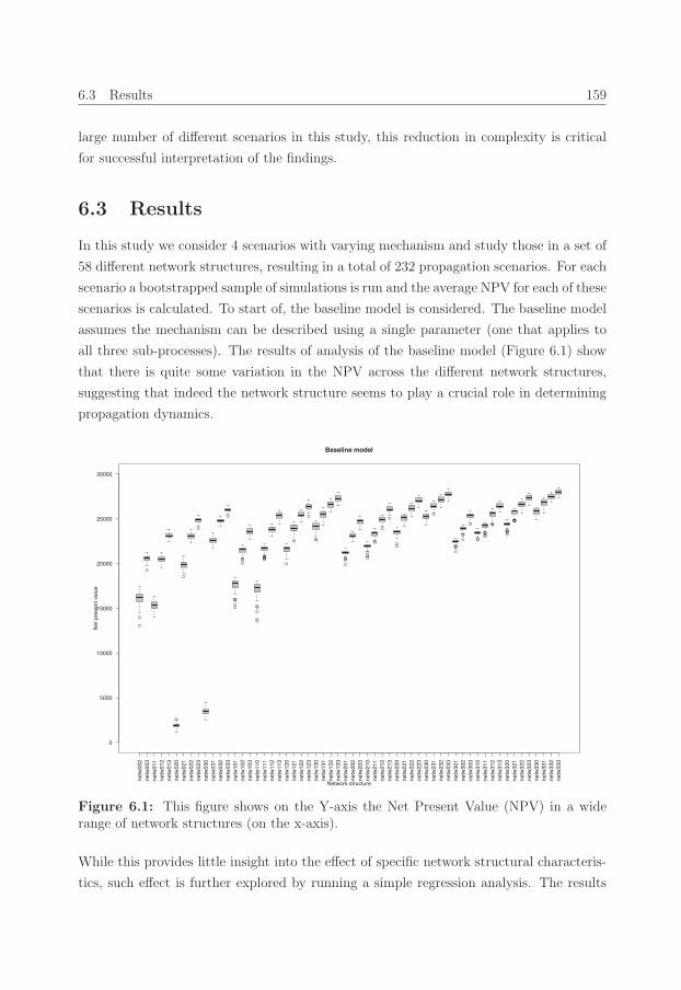
87_Erim_Vermeer Stand.job
6.3 Results 159
large number of different scenarios in this study, this reduction in complexity is critical
for successful interpretation of the findings.
6.3 Results
In this study we consider 4 scenarios with varying mechanism and study those in a set of
58 different network structures, resulting in a total of 232 propagation scenarios. For each
scenario a bootstrapped sample of simulations is run and the average NPV for each of these
scenarios is calculated. To start of, the baseline model is considered. The baseline model
assumes the mechanism can be described using a single parameter (one that applies to
all three sub-processes). The results of analysis of the baseline model (Figure 6.1) show
that there is quite some variation in the NPV across the different network structures,
suggesting that indeed the network structure seems to play a crucial role in determining
propagation dynamics.
●
●
●
●
●
●
●
●
●●
●●
●●●
●
●
●
●
●
●●●●●●
●
●
●
●●
●
●●●●●●●
●●
●
●
●●
●
●●
●
●
●●
●
●
●●
●●●●●
●●
●●●●●
●●●●●
netw
002
netw
003
netw
011
netw
012
netw
013
netw
020
netw
021
netw
022
netw
023
netw
030
netw
031
netw
032
netw
033
netw
101
netw
102
netw
103
netw
110
netw
111
netw
112
netw
113
netw
120
netw
121
netw
122
netw
123
netw
130
netw
131
netw
132
netw
133
netw
201
netw
202
netw
203
netw
210
netw
211
netw
212
netw
213
netw
220
netw
221
netw
222
netw
223
netw
230
netw
231
netw
232
netw
233
netw
301
netw
302
netw
303
netw
310
netw
311
netw
312
netw
313
netw
320
netw
321
netw
322
netw
323
netw
330
netw
331
netw
332
netw
333
0
5000
10000
15000
20000
25000
30000
Baseline model
Net
pre
sent
val
ue
Network structure
Figure 6.1: This figure shows on the Y-axis the Net Present Value (NPV) in a widerange of network structures (on the x-axis).
While this provides little insight into the effect of specific network structural characteris-
tics, such effect is further explored by running a simple regression analysis. The results
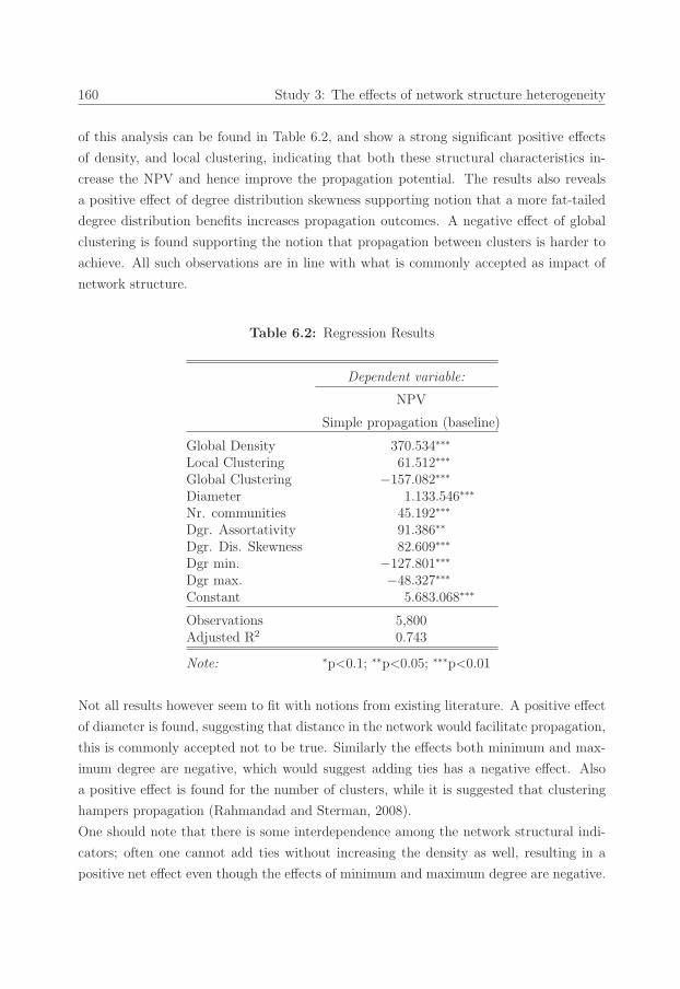
87_Erim_Vermeer Stand.job
160 Study 3: The effects of network structure heterogeneity
of this analysis can be found in Table 6.2, and show a strong significant positive effects
of density, and local clustering, indicating that both these structural characteristics in-
crease the NPV and hence improve the propagation potential. The results also reveals
a positive effect of degree distribution skewness supporting notion that a more fat-tailed
degree distribution benefits increases propagation outcomes. A negative effect of global
clustering is found supporting the notion that propagation between clusters is harder to
achieve. All such observations are in line with what is commonly accepted as impact of
network structure.
Table 6.2: Regression Results
Dependent variable:
NPV
Simple propagation (baseline)
Global Density 370.534∗∗∗
Local Clustering 61.512∗∗∗
Global Clustering −157.082∗∗∗
Diameter 1.133.546∗∗∗
Nr. communities 45.192∗∗∗
Dgr. Assortativity 91.386∗∗
Dgr. Dis. Skewness 82.609∗∗∗
Dgr min. −127.801∗∗∗
Dgr max. −48.327∗∗∗
Constant 5.683.068∗∗∗
Observations 5,800Adjusted R2 0.743
Note: ∗p<0.1; ∗∗p<0.05; ∗∗∗p<0.01
Not all results however seem to fit with notions from existing literature. A positive effect
of diameter is found, suggesting that distance in the network would facilitate propagation,
this is commonly accepted not to be true. Similarly the effects both minimum and max-
imum degree are negative, which would suggest adding ties has a negative effect. Also
a positive effect is found for the number of clusters, while it is suggested that clustering
hampers propagation (Rahmandad and Sterman, 2008).
One should note that there is some interdependence among the network structural indi-
cators; often one cannot add ties without increasing the density as well, resulting in a
positive net effect even though the effects of minimum and maximum degree are negative.
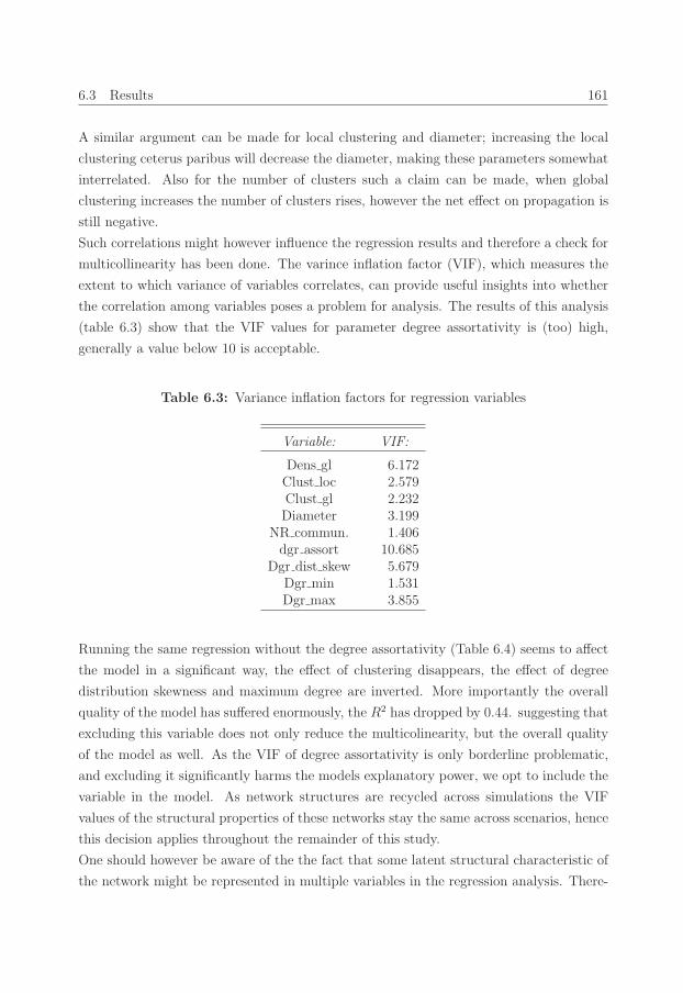
88_Erim_Vermeer Stand.job
6.3 Results 161
A similar argument can be made for local clustering and diameter; increasing the local
clustering ceterus paribus will decrease the diameter, making these parameters somewhat
interrelated. Also for the number of clusters such a claim can be made, when global
clustering increases the number of clusters rises, however the net effect on propagation is
still negative.
Such correlations might however influence the regression results and therefore a check for
multicollinearity has been done. The varince inflation factor (VIF), which measures the
extent to which variance of variables correlates, can provide useful insights into whether
the correlation among variables poses a problem for analysis. The results of this analysis
(table 6.3) show that the VIF values for parameter degree assortativity is (too) high,
generally a value below 10 is acceptable.
Table 6.3: Variance inflation factors for regression variables
Variable: VIF:
Dens gl 6.172Clust loc 2.579Clust gl 2.232Diameter 3.199
NR commun. 1.406dgr assort 10.685
Dgr dist skew 5.679Dgr min 1.531Dgr max 3.855
Running the same regression without the degree assortativity (Table 6.4) seems to affect
the model in a significant way, the effect of clustering disappears, the effect of degree
distribution skewness and maximum degree are inverted. More importantly the overall
quality of the model has suffered enormously, the R2 has dropped by 0.44. suggesting that
excluding this variable does not only reduce the multicolinearity, but the overall quality
of the model as well. As the VIF of degree assortativity is only borderline problematic,
and excluding it significantly harms the models explanatory power, we opt to include the
variable in the model. As network structures are recycled across simulations the VIF
values of the structural properties of these networks stay the same across scenarios, hence
this decision applies throughout the remainder of this study.
One should however be aware of the the fact that some latent structural characteristic of
the network might be represented in multiple variables in the regression analysis. There-
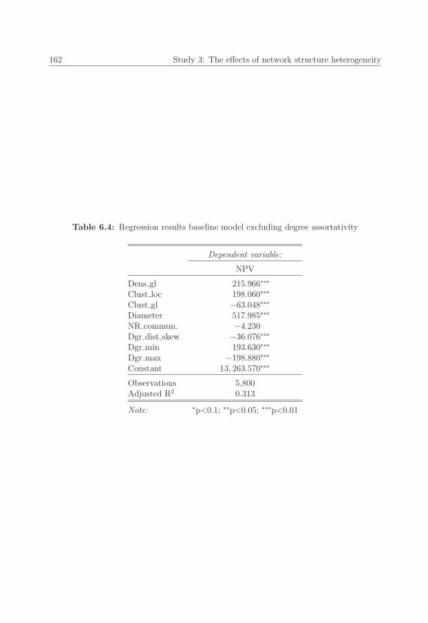
88_Erim_Vermeer Stand.job
162 Study 3: The effects of network structure heterogeneity
Table 6.4: Regression results baseline model excluding degree assortativity
Dependent variable:
NPV
Dens gl 215.966∗∗∗
Clust loc 198.060∗∗∗
Clust gl −63.048∗∗∗
Diameter 517.985∗∗∗
NR commun. −4.230Dgr dist skew −36.076∗∗∗
Dgr min 193.630∗∗∗
Dgr max −198.880∗∗∗
Constant 13, 263.570∗∗∗
Observations 5,800Adjusted R2 0.313
Note: ∗p<0.1; ∗∗p<0.05; ∗∗∗p<0.01

89_Erim_Vermeer Stand.job
6.3 Results 163
fore the interpretation of the regression results does require some caution in terms of
drawing conclusions on the effect of specific parameters. Regardless, the baseline model
as a whole has an adjusted R2 of 0.743 indicating that the dimensions of structure do
provide a good indication of propagation dynamics in this scenario.
The baseline model (Table 6.2) covers only a single mechanism of propagation, and many
of such mechanisms exist. As the mechanism propagation is claimed to play a role in the
propagation dynamics the baseline model is compared to three additional scenarios. Each
of these scenarios covers a propagation process with the same overarching propagation
probability, but with different decomposition into the three sub-processes of propagation.
Each scenario therefore has the same dyadic propagation dynamics, but a different mech-
anism of propagation. The results of the comparison (Figure 6.2) reveals no significant
differences among these scenarios, indicating that the propagation mechanism seems not
to affect the dynamics of propagation.
Figure 6.2: This figure shows on the Y-axis the Net Present Value (NPV) of processeswith different propagation dynamics (indicated by color) in a wide range of networkstructures (on the x-axis).

89_Erim_Vermeer Stand.job
164 Study 3: The effects of network structure heterogeneity
The subsequent regression results presented in Table 6.5 further corroborate the notion
that the effect of network structure is the same across all four scenarios.
Table 6.5: Regression results for a simple propagation mechanism
Dependent variable:
NPV
(Scenario 1) (Scenario 2) (Scenario 3) (Baseline)
Global Density 368.779∗∗∗ 370.126∗∗∗ 371.547∗∗∗ 370.534∗∗∗
Local Clustering 61.364∗∗∗ 61.155∗∗∗ 61.586∗∗∗ 61.512∗∗∗
Global Clustering −156.348∗∗∗ −156.612∗∗∗ −156.934∗∗∗ −157.082∗∗∗
Diameter 1, 131.935∗∗∗ 1, 128.468∗∗∗ 1, 138.710∗∗∗ 1, 133.546∗∗∗
Nr. Communities 45.106∗∗∗ 44.743∗∗∗ 43.669∗∗∗ 45.192∗∗∗
Dgr. assortativity 90.019∗∗∗ 90.904∗∗∗ 92.858∗∗∗ 91.386∗∗∗
Dgr. Dist. skewness 82.318∗∗∗ 83.575∗∗∗ 84.448∗∗∗ 82.609∗∗∗
Dgr. min −125.387∗∗∗ −127.874∗∗∗ −124.993∗∗∗ −127.801∗∗∗
Dgr. max −47.215∗∗∗ −47.376∗∗∗ −48.446∗∗∗ −48.327∗∗∗
Constant 5, 726.858∗∗∗ 5, 686.745∗∗∗ 5, 541.541∗∗∗ 5, 683.068∗∗∗
Observations 5,800 5,800 5,800 5,800Adjusted R2 0.743 0.743 0.744 0.743
Note: ∗p<0.1; ∗∗p<0.05; ∗∗∗p<0.01
This finding seems to contradict results indicating that variations in the propagation
mechanism, in some structures, yield different system-wide propagation dynamics (Cen-
tola and Macy, 2007). It should be noted that all models analyzed up until this point,
while varying in their decomposition, have adopted a relatively simple mechanism of prop-
agation. A simple mechanism implies that the propagation mechanism is unaffected by
any source of outside influence. In contrast, in more complex propagation mechanisms,
such as complex contagion (Centola and Macy, 2007), costly contagion and information
overflow, it assumed that the mechanism is influenced by the structure, and hence an
interaction effect between structure and the mechanism of propagation is present. The
existence of such an interaction effect is explored by comparing our baseline model to
models adopting these more complex propagation mechanisms. The full range analysis
scenarios can be found in tables 6.9, 6.12, 6.11, 6.10 and figures 6.3, 6.4, 6.5 presented in
the SI).
These results show that across the different types of complex propagation mechanisms a
strong variance in the propagation dynamics can be observed. When the regression results

90_Erim_Vermeer Stand.job
6.3 Results 165
of the scenario 1 across the different mechanisms (Table 6.6) are compared it can be ob-
served that the information overload and simple mechanisms are nearly similar, but that
they differ radically from the other two mechanisms (which also differ from each other).
The results indicate that the effects of local clustering, and the number of communities on
NPV have turned negative in the costly contagion mechanism. For the mechanism of com-
plex contagion the diameter, degree assortativity, and degree distribution skewness now
have a negative effect on NPV, whereas the effect of minimum degree has turned positive.
Also the effect of the maximum degree has disappeared altogether. These results suggest
that the effects of some of the network structural characteristics vary significantly across
different types of mechanism. Therefore these results refute the notion that the effects
of network structure are constant, and give merit to the notions that the propagation
dynamics are conditional upon the mechanism used. This supports the claim (Centola
and Macy, 2007; Aral et al., 2013) that the mechanism of propagation is a key driver of
propagation dynamics.
Table 6.6: Regression results for scenario 1 under different mechanism of propagation
Dependent variable:
NPV
(Scenario 1) (Scenario 1) (Scenario 1) Scenario 1
Complex Contagion Costly Contagion Information Overload Simple
Global Density 338.579∗∗∗ 225.797∗∗∗ 369.771∗∗∗ 368.779∗∗∗
Local Clustering 101.405∗∗∗ −70.179∗∗∗ 61.233∗∗∗ 61.364∗∗∗
Global Clustering −150.677∗∗∗ −47.473∗∗∗ −156.592∗∗∗ −156.348∗∗∗
Diameter −398.234∗∗∗ 978.281∗∗∗ 1.130, 909∗∗∗ 1, 131.935∗∗∗
Nr. Communities 19.916∗∗∗ −9.404∗∗∗ 43.873∗∗∗ 45.106∗∗∗
Dgr. assortativity −171.151∗∗∗ 112.655∗∗∗ 93.450∗∗∗ 90.019∗∗∗
Dgr. Dist. skewness −114/289∗∗∗ 64.000∗∗∗ 83.263∗∗∗ 82.318∗∗∗
Dgr. min 98.366∗∗∗ −113.618∗∗∗ −128.079∗∗∗ −125.387∗∗∗
Dgr. max 3.760 −50.000∗∗∗ −49.712∗∗∗ −47.215∗∗∗
Constant 10, 280.770∗∗∗ 2, 384.362∗∗∗ 5, 637.771∗∗∗ 5, 726.858∗∗∗
Observations 5,800 5,800 5,800 5,800Adjusted R2 0.898 0.855 0.742 0.743
Note: ∗p<0.1; ∗∗p<0.05; ∗∗∗p<0.01
Not only between the mechanism types, but also within these types variance in the dynam-
ics and the effects of network structure can be observed. This indicates that, in contrast
to the simple propagation setting, in complex propagation settings the decomposition
of the mechanism plays a critical role in determining the propagation dynamics. This
is particularly apparent when considering the costly contagion and complex contagion
mechanisms.
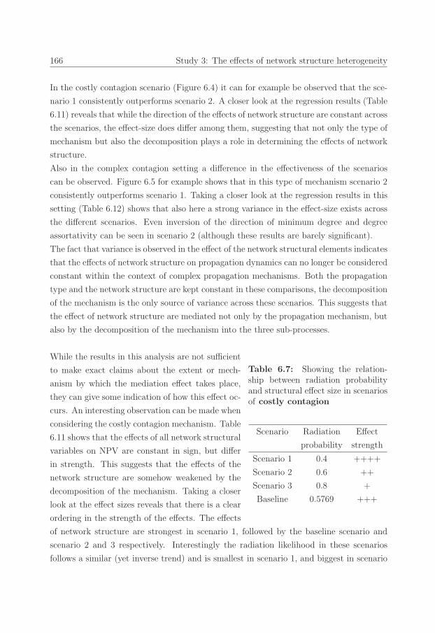
90_Erim_Vermeer Stand.job
166 Study 3: The effects of network structure heterogeneity
In the costly contagion scenario (Figure 6.4) it can for example be observed that the sce-
nario 1 consistently outperforms scenario 2. A closer look at the regression results (Table
6.11) reveals that while the direction of the effects of network structure are constant across
the scenarios, the effect-size does differ among them, suggesting that not only the type of
mechanism but also the decomposition plays a role in determining the effects of network
structure.
Also in the complex contagion setting a difference in the effectiveness of the scenarios
can be observed. Figure 6.5 for example shows that in this type of mechanism scenario 2
consistently outperforms scenario 1. Taking a closer look at the regression results in this
setting (Table 6.12) shows that also here a strong variance in the effect-size exists across
the different scenarios. Even inversion of the direction of minimum degree and degree
assortativity can be seen in scenario 2 (although these results are barely significant).
The fact that variance is observed in the effect of the network structural elements indicates
that the effects of network structure on propagation dynamics can no longer be considered
constant within the context of complex propagation mechanisms. Both the propagation
type and the network structure are kept constant in these comparisons, the decomposition
of the mechanism is the only source of variance across these scenarios. This suggests that
the effect of network structure are mediated not only by the propagation mechanism, but
also by the decomposition of the mechanism into the three sub-processes.
Table 6.7: Showing the relation-ship between radiation probabilityand structural effect size in scenariosof costly contagion
Scenario Radiation Effect
probability strength
Scenario 1 0.4 ++++
Scenario 2 0.6 ++
Scenario 3 0.8 +
Baseline 0.5769 +++
While the results in this analysis are not sufficient
to make exact claims about the extent or mech-
anism by which the mediation effect takes place,
they can give some indication of how this effect oc-
curs. An interesting observation can be made when
considering the costly contagion mechanism. Table
6.11 shows that the effects of all network structural
variables on NPV are constant in sign, but differ
in strength. This suggests that the effects of the
network structure are somehow weakened by the
decomposition of the mechanism. Taking a closer
look at the effect sizes reveals that there is a clear
ordering in the strength of the effects. The effects
of network structure are strongest in scenario 1, followed by the baseline scenario and
scenario 2 and 3 respectively. Interestingly the radiation likelihood in these scenarios
follows a similar (yet inverse trend) and is smallest in scenario 1, and biggest in scenario

91_Erim_Vermeer Stand.job
6.4 Implications 167
3 (Table 6.7). While this in no way provides proof of causality this observation does
suggests that, for costly contagion, there is a negative correlation between the effects of
network structure, and the probability of radiation. Exploring this relationship would be
a viable extension of this research.
6.4 Implications
This study has focused in the role of the propagation mechanism in impacting the relation-
ship between the network structure and propagation dynamics. By adopting an actor level
information processing view and taking a closer look at what happens during propagation
the mechanism of propagation has been decomposed into three sub-processes: Radiation,
Transmission and Reception, and the effects of doing so have been explored. In doing so
this study has made three contribution to the literature on propagation specifically and
network research in general.
First, by building on the work of Jackson and Rogers (2007) and extending their hybrid
model of network formation a new model for generating synthetic network structures has
been put forward. This model allows for generating networks with a wide range of net-
work characteristics, covering the space of network structural parameters from regular
ring networks towards small-world and scale-free network (and all which lies in between).
In doing so it provides a solid basis for generating synthetic network structure which re-
semble network structures observed in practice.
Second, this study has shown that the mechanism of propagation is a key driver of propa-
gation dynamics on the system level. Significant variance in propagation dynamics across
different type of more complex mechanisms has been found proving the importance of
the considering mechanism of propagation in determining and understanding propagation
dynamics.
Third, by exploring different mechanism across a wide array of networks with varying
structural characteristics, it has been shown that the effect of network structure are
constant only in scenarios with simple propagation mechanisms. When more complex
mechanism of propagation are adopted the a single network structure can yield various
propagation dynamics, suggesting that the effect of network structure is conditional on
the mechanism of propagation.

91_Erim_Vermeer Stand.job
168 Study 3: The effects of network structure heterogeneity
This finding indicates a clear boundary to the generalizability of the effects of network
structure on propagation dynamics. Whereas existing literature is largely supported in
their findings on the impact of network structure, our findings suggest that these findings
only hold under a simple propagation mechanism. When more complex mechanisms of
propagation are adopted the impact of network structure might significantly change. This
conclusion is in line with the conclusion drawn in previous work on complex contagion
(Centola and Macy, 2007). In studying more complex mechanisms of propagation it is
therefore a prerequisite to know the decomposition of the mechanism and understand the
role of each of the sub-process of propagation.
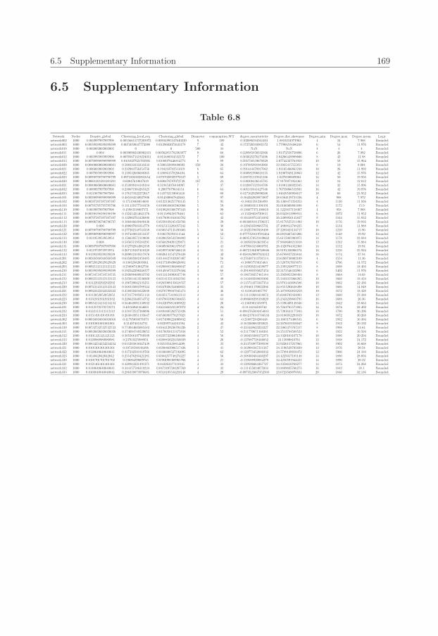
92_Erim_Vermeer Stand.job
6.5 Supplementary Information 169
6.5 Supplementary Information
Table 6.8
Network Nodes Density global Clustering local avg Clustering global Diameter communities WT degree assortativity Degree dist skewness Degree min Degree max Degree mean Logicnetwork002 1000 0.003997997997998 0.00556615737203972 0.00934995547640249 9 109 0.102086594561404 1.8810234973963 4 34 7.988 Boundednetwork003 1000 0.00599399399399399 0.0074059047772098 0.0129602073633178 7 42 0.172720593905572 1.77998219486248 6 54 11.976 Boundednetwork010 1000 0.002002002002002 0 0 500 34 NaN NaN 4 4 4 Boundednetwork011 1000 0.004 0.00390902430902431 0.00562851782363977 9 68 0.228985850332366 1.91372556750096 6 26 7.992 Boundednetwork012 1000 0.005995995995996 0.00705671419224051 0.013486934532172 7 100 0.303625276173496 2.04266449989606 8 42 11.98 Boundednetwork013 1000 0.00798998998998999 0.0101027921703905 0.0180079446814771 6 89 0.295758559678829 2.07742327761958 10 58 15.964 Boundednetwork020 1000 0.00400600600600601 0.500333333333333 0.500332889480692 250 28 0.197995991983968 22.2935417555851 8 10 8.004 Boundednetwork021 1000 0.006002002002002 0.232904756354756 0.194233782513319 8 65 0.291444478917062 1.91165466861238 10 26 11.992 Boundednetwork022 1000 0.007995995995996 0.139532686680365 0.108861578266494 6 64 0.360981996618155 1.91907949110863 12 42 15.976 Boundednetwork023 1000 0.00998798798798799 0.0973303302801654 0.0787920929770537 5 69 0.388781119321166 1.6270100689063 14 50 19.956 Boundednetwork030 1000 0.00601201201201201 0.60047619047619 0.600478787072749 167 24 0.330308436545785 17.9170971954461 12 16 12.012 Boundednetwork031 1000 0.00800600600600601 0.353899184149184 0.319453076444997 7 37 0.332087321934708 1.81801336022345 14 32 15.996 Boundednetwork032 1000 0.009997997997998 0.238671904265325 0.20077679634154 6 64 0.405131641427346 1.76759066519591 16 42 19.976 Boundednetwork033 1000 0.011987987987988 0.176173322272617 0.145732159601416 5 69 0.417162929890286 1.84639530958617 18 60 23.952 Boundednetwork101 1000 0.00398998998998999 0.485584550027806 0.014500667842463 7 97 -0.164242828873807 28.6564139731336 4 988 7.972 Boundednetwork102 1000 0.00597397397397397 0.17519468054689 0.0122136257793135 5 95 -0.14031591236499 26.1368471354253 4 1130 11.936 Boundednetwork103 1000 0.00795795795795796 0.131129177583359 0.0169638682962666 5 59 -0.106093311398191 26.0166909801898 6 1172 15.9 Boundednetwork110 1000 0.003997997997998 0.45983538607571 0.0190283366797443 6 99 -0.136677371190819 31.5225657158367 4 958 7.988 Boundednetwork111 1000 0.00598198198198198 0.132414214645176 0.011589458176461 5 63 -0.13328658720813 26.0343813998911 6 1072 11.952 Boundednetwork112 1000 0.00797397397397397 0.132902763426898 0.0179091163033782 5 42 -0.104169743351692 26.2409956145827 8 1164 15.932 Boundednetwork113 1000 0.00996796796796797 0.106846649489436 0.0228439245450766 4 29 -0.0836091812796215 25.8179525211492 10 1176 19.916 Boundednetwork120 1000 0.006 0.490697603314778 0.0315151201057241 5 38 -0.129456508665731 27.4808811788225 8 1134 11.988 Boundednetwork121 1000 0.00798798798798799 0.277202148743359 0.0305547135495605 5 56 -0.102257867038498 27.2285023134717 10 1210 15.96 Boundednetwork122 1000 0.00996996996996997 0.197410012355237 0.036576393511544 4 52 -0.0777321619785464 26.6859467455266 12 1148 19.92 Boundednetwork123 1000 0.011953953953954 0.156639572119698 0.0396250532594802 4 51 -0.0695170521839662 25.6115085903971 14 1178 23.884 Boundednetwork130 1000 0.008 0.545651595583291 0.0568294091229871 4 21 -0.100502343619354 27.9048608211018 12 1232 15.984 Boundednetwork131 1000 0.00997997997997998 0.352792844962359 0.0609363961379547 4 41 -0.079563158069781 26.4320764352368 14 1152 19.94 Boundednetwork132 1000 0.011973973973974 0.267159167418328 0.0599716967466116 4 55 -0.0672136490740846 26.9191330066574 16 1216 23.924 Boundednetwork133 1000 0.0139339339339339 0.209012410517876 0.0626131547276438 4 42 -0.0581629097924312 25.6788837233844 18 1174 27.84 Boundednetwork201 1000 0.00568568568568569 0.635805982458485 0.0144427832087407 4 58 -0.276307313791514 23.6269730002109 4 1554 11.36 Boundednetwork202 1000 0.00729329329329329 0.33832382639361 0.0157109496626881 4 71 -0.18985755015463 25.5287917655673 6 1706 14.572 Boundednetwork203 1000 0.00921121121121121 0.25808743042736 0.0208881304880647 4 41 -0.145926234458677 25.2395248077155 8 1698 18.404 Boundednetwork210 1000 0.00599399399399399 0.592342296248377 0.0149587312378504 3 68 -0.291800195027474 22.3173546332901 6 1402 11.976 Boundednetwork211 1000 0.00734734734734735 0.292099409932792 0.0153124993037748 4 57 -0.186739257465144 25.2929952280483 8 1664 14.68 Boundednetwork212 1000 0.00922122122122122 0.245014413536969 0.0214122110162581 4 49 -0.143449248691006 25.2433315066265 10 1668 18.424 Boundednetwork213 1000 0.0112292292292292 0.196720042135251 0.0265909133618557 4 57 -0.115714373347354 24.9781443694586 10 1662 22.436 Boundednetwork220 1000 0.00743143143143143 0.568335003789144 0.0247026354660655 4 35 -0.191661170022266 24.8551204638498 10 1666 14.848 Boundednetwork221 1000 0.00922322322322322 0.358950281622038 0.0276799947945473 4 46 -0.14186481687797 25.4878950858259 10 1672 18.428 Boundednetwork222 1000 0.0112052052052052 0.272177895951133 0.0335175419612112 4 44 -0.111132683418072 25.6040702434981 12 1660 22.388 Boundednetwork223 1000 0.0131931931931932 0.226623340554752 0.0378653963504655 4 63 -0.096608298194929 25.2343239683795 16 1688 26.36 Boundednetwork230 1000 0.00934134134134134 0.564648081330932 0.0432079814089822 4 20 -0.13639013358971 25.5596409149346 14 1642 18.664 Boundednetwork231 1000 0.0112572572572573 0.40124941564603 0.0453463235387072 4 24 -0.1114214838742 25.7241765571865 14 1674 22.492 Boundednetwork232 1000 0.0132112112112112 0.319172527269096 0.0493405262752426 4 51 -0.0943765693454041 25.7201631177943 18 1700 26.396 Boundednetwork233 1000 0.0151491491491491 0.263843951135647 0.0536993778217021 4 44 -0.0842170145746533 24.8186952291659 18 1672 30.268 Boundednetwork302 1000 0.00816016016016016 0.41795050578373 0.0174990224009832 3 56 -0.21687250206448 24.1685171466531 6 1932 16.304 Boundednetwork303 1000 0.0101061061061061 0.3140746534731 0.022997344101594 4 43 -0.163360083292621 24.2676019350047 8 1912 20.192 Boundednetwork310 1000 0.00732732732732733 0.774044605065583 0.0164129236704326 2 37 -0.333448623224327 22.5065375767317 8 1998 14.64 Boundednetwork311 1000 0.00826026026026026 0.374094749229052 0.0176050121475834 3 52 -0.211770671168261 24.2513784588523 8 1922 16.504 Boundednetwork312 1000 0.0101121121121121 0.305568197769509 0.0235722906106686 4 56 -0.160433360172373 24.3320163167178 10 1886 20.204 Boundednetwork313 1000 0.0120980980980981 0.23763325988951 0.0288850224356039 4 26 -0.127687728446052 24.15090816761 12 1838 24.172 Boundednetwork320 1000 0.00834234234234234 0.615203838247439 0.025105438814499 3 33 -0.213750977209598 23.9226157257965 10 1902 16.668 Boundednetwork321 1000 0.0101301301301301 0.39738590146396 0.0280462986517426 3 41 -0.162994167211567 24.1190539705029 12 1876 20.24 Boundednetwork322 1000 0.0120640640640641 0.317232501819768 0.0336808527192095 3 62 -0.129773452040332 24.5789149910472 12 1906 24.104 Boundednetwork323 1000 0.014042042042042 0.255476293421281 0.0384257748274227 4 56 -0.108369484440297 24.4225017185148 14 1880 28.056 Boundednetwork330 1000 0.0101701701701702 0.59686499609745 0.0392098369965766 4 21 -0.159588920884279 24.4250591944431 14 1890 20.32 Boundednetwork331 1000 0.0121461461461461 0.428943221491271 0.043263377110165 4 33 -0.129596664367727 24.3358610768277 14 1874 24.268 Boundednetwork332 1000 0.0140640640640641 0.344157586319224 0.0472497594207769 4 32 -0.111455024075933 23.8889035766273 16 1842 28.1 Boundednetwork333 1000 0.0160840840840841 0.286359873976681 0.0518105534210148 4 29 -0.0973523667352503 23.6723569070581 20 1846 32.136 Bounded
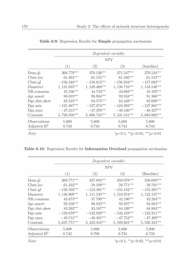
92_Erim_Vermeer Stand.job
170 Study 3: The effects of network structure heterogeneity
Table 6.9: Regression Results for Simple propagation mechanism
Dependent variable:
NPV
(1) (2) (3) (baseline)
Dens gl 368.779∗∗∗ 370.126∗∗∗ 371.547∗∗∗ 370.534∗∗∗
Clust loc 61.364∗∗∗ 61.155∗∗∗ 61.586∗∗∗ 61.512∗∗∗
Clust gl −156.348∗∗∗ −156.612∗∗∗ −156.934∗∗∗ −157.082∗∗∗
Diameter 1, 131.935∗∗∗ 1, 128.468∗∗∗ 1, 138.710∗∗∗ 1, 133.546∗∗∗
NR commun. 45.106∗∗∗ 44.743∗∗∗ 43.669∗∗∗ 45.192∗∗∗
dgr assort 90.019∗∗∗ 90.904∗∗∗ 92.858∗∗∗ 91.386∗∗∗
Dgr dist skew 82.318∗∗∗ 83.575∗∗∗ 84.448∗∗∗ 82.609∗∗∗
Dgr min −125.387∗∗∗ −127.874∗∗∗ −124.993∗∗∗ −127.801∗∗∗
Dgr max −47.215∗∗∗ −47.376∗∗∗ −48.446∗∗∗ −48.327∗∗∗
Constant 5, 726.858∗∗∗ 5, 686.745∗∗∗ 5, 541.541∗∗∗ 5, 683.068∗∗∗
Observations 5,800 5,800 5,800 5,800Adjusted R2 0.743 0.743 0.744 0.743
Note: ∗p<0.1; ∗∗p<0.05; ∗∗∗p<0.01
Table 6.10: Regression Results for Information Overload propagation mechanism
Dependent variable:
NPV
(1) (2) (3) (Baseline)
Dens gl 369.771∗∗∗ 337.894∗∗∗ 359.978∗∗∗ 358.689∗∗∗
Clust loc 61.233∗∗∗ 58.189∗∗∗ 59.771∗∗∗ 59.791∗∗∗
Clust gl −156.592∗∗∗ −152.491∗∗∗ −155.182∗∗∗ −155.391∗∗∗
Diameter 1, 130.909∗∗∗ 1, 111.535∗∗∗ 1, 124.954∗∗∗ 1, 122.137∗∗∗
NR commun. 43.873∗∗∗ 37.790∗∗∗ 42.190∗∗∗ 42.284∗∗∗
dgr assort 93.450∗∗∗ 96.833∗∗∗ 93.927∗∗∗ 94.884∗∗∗
Dgr dist skew 83.263∗∗∗ 83.587∗∗∗ 84.430∗∗∗ 84.884∗∗∗
Dgr min −128.079∗∗∗ −132.829∗∗∗ −133.459∗∗∗ −132.311∗∗∗
Dgr max −49.712∗∗∗ −48.401∗∗∗ −47.752∗∗∗ −47.409∗∗∗
Constant 5, 637.771∗∗∗ 5, 422.318∗∗∗ 5, 593.661∗∗∗ 5, 530.324∗∗∗
Observations 5,800 5,800 5,800 5,800Adjusted R2 0.742 0.709 0.734 0.733
Note: ∗p<0.1; ∗∗p<0.05; ∗∗∗p<0.01

93_Erim_Vermeer Stand.job
6.5 Supplementary Information 171
Table 6.11: Regression results for Costly Contagion propagation mechanism
Dependent variable:
NPV
(1) (2) (3) (4)
Dens gl 255.797∗∗∗ 184.505∗∗∗ 140.947∗∗∗ 191.757∗∗∗
Clust loc −70.179∗∗∗ −72.274∗∗∗ −66.078∗∗∗ −71.446∗∗∗
Clust gl −47.473∗∗∗ −33.438∗∗∗ −24.226∗∗∗ −35.056∗∗∗
Diameter 978.281∗∗∗ 714.467∗∗∗ 526.428∗∗∗ 751.296∗∗∗
NR commun. −9.404∗∗∗ −2.963∗ 0.840 −2.522dgr assort 112.655∗∗∗ 80.617∗∗∗ 56.792∗∗∗ 84.996∗∗∗
Dgr dist skew 64.000∗∗∗ 42.476∗∗∗ 27.183∗∗∗ 43.869∗∗∗
Dgr min −113.618∗∗∗ −70.001∗∗∗ −41.620∗∗∗ −73.809∗∗∗
Dgr max −50.000∗∗∗ −35.254∗∗∗ −24.238∗∗∗ −37.919∗∗∗
Constant 2, 384.362∗∗∗ 2, 965.865∗∗∗ 2, 959.129∗∗∗ 2, 833.484∗∗∗
Observations 5,800 5,800 5,800 5,800Adjusted R2 0.855 0.859 0.862 0.855
Note: ∗p<0.1; ∗∗p<0.05; ∗∗∗p<0.01
Table 6.12: Regression results for Complex contagion propagation mechanism
Dependent variable:
NPV
(1) (2) (3) (4)
Dens gl 338.579∗∗∗ 582.286∗∗∗ 457.137∗∗∗ 475.090∗∗∗
Clust loc 101.405∗∗∗ 110.658∗∗∗ 108.068∗∗∗ 110.160∗∗∗
Clust gl −150.677∗∗∗ −251.107∗∗∗ −200.524∗∗∗ −204.589∗∗∗
Diameter −398.234∗∗∗ −559.506∗∗∗ −493.917∗∗∗ −488.156∗∗∗
NR commun. 19.916∗∗∗ 41.856∗∗∗ 27.921∗∗∗ 31.265∗∗∗
dgr assort −171.151∗∗∗ 17.079∗∗ −115.301∗∗∗ −99.497∗∗∗
Dgr dist skew −114.289∗∗∗ 0.710 −73.789∗∗∗ −66.200∗∗∗
Dgr min 98.366∗∗∗ −24.487∗ 56.170∗∗∗ 55.725∗∗∗
Dgr max 3.760 −114.356∗∗∗ −42.677∗∗∗ −50.976∗∗∗
Constant 10, 280.770∗∗∗ 8, 009.745∗∗∗ 10, 291.560∗∗∗ 9, 666.867∗∗∗
Observations 5,800 5,800 5,800 5,800Adjusted R2 0.898 0.888 0.915 0.912
Note: ∗p<0.1; ∗∗p<0.05; ∗∗∗p<0.01
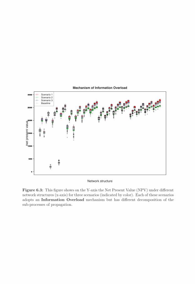
93_Erim_Vermeer Stand.job
●
●
●●
●●
●
●
●●
●
●
●
●
●●●●●
●●●
●●●●
●●●●
●
●●●
●
●
●●
●
●
●
●●●●●●
●●
●●
●●
●●
●●●●●
●●
●●●
●
●●● ●
●
●●●●
●●
●●●
●●
●●●●●●
●
●●●●
●
●●
●●
0
5000
10000
15000
20000
25000
30000
Mechanism of Information Overload
Network structure
Net
pre
sent
val
ue
●●●●●
● ●
●
●
●●
●
●
●●
●
●
●
●
●
●
●
●●●●
●●●●
●●●●
●●●● ●
●
●●
●
●●
●
●●●●●
●●●● ●●●
●●
●●
●●●
●●
●
●●●
●●
●●
●
●
●
●●●●
●●
0
5000
10000
15000
20000
25000
30000
●●
●
●
●●
●
● ●●●
●●●●
●●
●
●●
●
●●
●
●
●●●
●
●●
●
●●
● ●
●
●
●●●●
●●●●●
●●●
●
●
●●●
●●●
●●
●
●●●●●●●
●●●●●●
●
●
●●●●●
●●
●
●
●●
0
5000
10000
15000
20000
25000
30000
●●
●
●
●
●
●
●
●
●●●
●●
●●
●
●
●●●●
●
●●
●●●●
●●●
●●●●
●●●
●
●● ●●●●●
●●
●
●
●●●●
●●●●●
●●●●●●●●●●
●●
●●●●●
●●●●
●
●●
0
5000
10000
15000
20000
25000
30000 ●
●
●
●
Scenario 1Scenario 2Scenario 3Baseline
Figure 6.3: This figure shows on the Y-axis the Net Present Value (NPV) under differentnetwork structures (x-axis) for three scenarios (indicated by color). Each of these scenariosadopts an Information Overload mechanism but has different decomposition of thesub-processes of propagation.

94_Erim_Vermeer Stand.job
●●
●●●●
●
●●
●
●
●
●
●
●
●●●
●
●
●
●●
●
●
●
●
●
●●
●
●
●
●
●●
●
●
●●
●
●
●● ●
●
●●●
●
●
●
●●
0
5000
10000
15000
20000
25000
30000
Mechanism of Costly Contagion
Network structure
Net
pre
sent
val
ue
●●
●●
●●● ●
●●●●
●
●
●●●
●
●
●●●
●●
●●
●●
●
●
●
●●●
●
●
●
●●
●
● ●
●
●
●●●
●●
●●●● ●
●
●
●
●
●
●
●●●
●●
●
●
●
0
5000
10000
15000
20000
25000
30000
●
●●
●●●
●
●●
●●
●●●
●●
●
●●
●
●●●
● ●
●●
●
●
●
●●
●
●●
●
●
●●
●
●●●
●●
●
●●
●●
●
●
●
●
●●●
●
●
●
●
●●
0
5000
10000
15000
20000
25000
30000
●
●
●
●
●●
●●
● ●●
●
●
●
●
●●
●
●●
●
●●
●
●
● ●●
●
●●
●●
●
●●
●
●●
●
●
●
●
●
●
●
●
●●
●●
●●
●
●●
●
●
●●
●
●
●●●
●
●
●
●
●
●
0
5000
10000
15000
20000
25000
30000 ●
●
●
●
Scenario 1Scenario 2Scenario 3Baseline
Figure 6.4: This figure shows on the Y-axis the Net Present Value (NPV) under differentnetwork structures (x-axis) for three scenarios (indicated by color). Each of these scenariosadopts a Costly Contagion mechanism but has different decomposition of the sub-processes of propagation.

94_Erim_Vermeer Stand.job
● ●●●●●●● ●●●●●●●●
●●
●●●
●
●
●●
●●●
●
●
●
●
●
●
●●
●●●●
●●
●●
●●●
●
●
●
●
●
●
●
●●
●
●
●
●●●
●
●●
●●
●
●
●
●
●
●●●●●●●
●
●
●●●
●●
●
●●
●
●
●
●
●●●●●●●●
●
●●●
●●●●●●●●
●●●●●
●
●
●●
●●
●●
●
●●●
●
●
●
●●
●
●
●
●●
●
●●●●●
●
●
●
●
●●
●
●●
●● ●
●
●●
●
●●
●
●
●
●
●
●
●
●
●
●
●●
●
●
●
●
●●
●
●
●
●
●●
●
●●
●
●
●
●
●
●
●●
●
●
●●
●
●
●
●
● ●●
●●
●
●●
●
●
●
●
●
●
●
●
●●
●
●
●
0
5000
10000
15000
20000
25000
30000
Mechanism of Complex Contagion
Network structure
Net
pre
sent
val
ue
●
●●
●
●●●
●
●●●
●
●
●
●
●
●
●
●
●
●●
●
●
●
●
●
●●
●
●
●
●
●
●
●
●●
●
●
●●
●
●
●
●
●
●
●
●
●
●●
●
●●
●
●
●●●
●
●
●
●●●●●●●●●●●●●●
●
●
●
●● ●●●●●●●●●●●
●
●●●
●
●
●
●
●●
●
●●
●●
●
●
●●●
●●●●
●
●
●
●
●
●
●●
●
●●
●
●
●
●●●
●
●
●
●
●
●●
●●
●●
●●
●●
●
●
●
●
●●
●●
●●●●
●
●
●
●●
●
●
●
●
0
5000
10000
15000
20000
25000
30000
●
●
●
●●
●
●
●
●
●●●
●
●
●●
●
●
●
●
●
●
●
●
●
●
●
●●
●
●
●
●
●
●●
●●●
●
●
●
●
●
●●●
●
●
●●
●
●
●
●
●
●
●
●●●●●●●
●
●●●●●●
●●●●●●
●●●●
●●
●
●
●●● ●●
●●
●●
●●
●
●
●
●
●
●●
●
●
●
●●
●
●
●●
●
●
●
●●
●
●
●●
●
●
●
●
●
●●
●●
●
●
●
●
●
●
●
●●
●
●●
●
●●
●
●
●
● ●
●
●
●
●
●
●●● ●
●●
●
●●●●●
●
●
●●
●●
●
●●●
●
●●
●●●
●
●
0
5000
10000
15000
20000
25000
30000
●●●●●
●
●●
●
●●● ●
●●
●●●●
●
●●
●
●
●
●
●
●●
●
●
●
●
●
●
●●●
●●●●●●
●
●
●
●
●
●
●
●
●●
●
●
●
●
●●●
●●●●●●●
●●●●●●●● ●
●
●
●
●
●
●
●●●
●
●●●●
●
●
●
●
●●●
●●●
●
●
●
●
●●
●
●
●●
●
●●
●●
●●
●
●
●
●
●
●●
●
●
●
●
●
●●●
●
●
●
●
●
●
●
●●
●●●
●
●
●
●●
●
●
●
●●●
●
●●
●
●●
●
●
●●●●● ●
●●●●
●
●
●
●
●
●
●●
●●
●●●●
●●
●●
●
0
5000
10000
15000
20000
25000
30000 ●
●
●
●
Scenario 1Scenario 2Scenario 3Baseline
Figure 6.5: This figure shows on the Y-axis the Net Present Value (NPV) under differentnetwork structures (x-axis) for three scenarios (indicated by color). Each of these scenariosadopts a Complex Contagion mechanism but has different decomposition of the sub-processes of propagation.
95_Erim_Vermeer Stand.job
Chapter 7
Summary and Conclusion
This dissertation aimed to show the impact of the propagation mechanism on propaga-
tion dynamics. It has done so by introducing a framework which considers the direct
impact of the mechanism of propagation on propagation dynamics, and the interaction
effect of this mechanism with the other drivers of propagation dynamics; the seed of in-
fection and the network structure. This has resulted in three research questions, which
subsequently have been the focus of the three studies executed in this dissertation. This
chapter will revisit these research questions, and their answers, and will synthesized them
into a discussion on the lessons learned with regards to the impact of the mechanism of
propagation. Furthermore it will provide a reflection on this discussion focusing on the
implications, limitations and future research.
The mechanism of propagation has been studied by adopting the information processing
view of propagation. This view, introduced in chapter 2 and 4, considers propagation to
be a process which consist of information processing at the actor level. The main research
question in this dissertation therefore is:
(How) do differences in the information processing at the actor level affect
system-wide propagation dynamics?
The answer provided to this question in this dissertation is that the propagation mecha-
nism indeed is an important driver of propagation dynamics. Adopting the information
processing view, which captures such mechanism and describes it by means of three actor
level information sub-processes, provides a useful method for studying propagation dy-
namics on the system level. It has been shown that the decomposition of the mechanism
of propagation and identifying the information processing behavior on the actor level is
key in determining the effects of interventions, network structure, and heterogeneity in
95_Erim_Vermeer Stand.job
176 Summary and Conclusion
actor behavior.
It has been found that actor level information processing behavior does not have added
value in all scenarios. In scenarios with homogenous or simple propagation mechanisms
the propagation dynamics seem to be unaffected by the differences in actor level informa-
tion processing. Models are by design an abstraction of reality, and the goal is often to
keep the models as simple as possible, for this reason modeling propagation by means of
a traditional models is a valid choice, in scenarios in which one considers a propagation
process with a simple mechanism, and as long as both the effectiveness of interventions
and the impact of local heterogeneity are irrelevant.
It should be noted that the propagation mechanisms in practice are likely to be far more
complex than assumed in such models. Often the mechanism will vary locally and be
dependent on outside factors. This dissertation has shown that under such conditions the
decomposition of the propagation mechanism is critical to consider. In such settings the
information processing on the actor level will locally affect the propagation mechanism,
resulting in heterogeneity in local dynamics. This heterogeneity in turn is essential in
order to understand and effectively model propagation dynamics on the system level. It
is therefore highly desirable to adopt an information processing view of propagation.
In order to substantiate these conclusions, a recap of the three studies in this dissertation
and an discussion on their findings is provided next. The first study in this dissertation
(chapter 4) aimed to address part of the primary research question; it focuses on the
whether any impact exists of actor level information processing behavior of system-wide
propagation dynamics. The question how such impact occurs is covered in the second
and third study in this dissertation.
7.1 Study 1
To show the effect of differences in actor level information processing, the first study
(chapter 4) provides a translation of the information processing view of propagation into
a model of propagation. This model considers propagation as a local process which takes
place at the actor level and by doing places emphasis especially on the mechanism of
propagation. It describes the mechanism of propagation by means of three sub-processes
which occur between actors; Radiation, Transmission and Reception, resulting in the
96_Erim_Vermeer Stand.job
7.1 Study 1 177
RTR-model of propagation.
Adopting a new model of propagation (such as the RTR-model) first and foremost re-
quires validation. Not only should it be shown that the RTR-model is a valid method
for studying propagation in a different way, but also that adopting a different approach
indeed makes sense; that it is a difference which makes a difference. Validation of the
RTR-model of propagation therefore rests upon two pillars; the model needs to be method-
ological sound, and it needs to be practically relevant.
The first part of study 1 has tested the ability of the RTR-model to describe propagation
phenomena. Field data of the adoption of a mobile phone application (Yahoo! GO 2.0)
is used as an example of a propagation phenomenon. This data describes the adoption of
Yahoo! GO 2.0 among a network of Yahoo! messenger users, and hence considers prop-
agation in a networked setting. The performance of the RTR-model in describing this
adoption process is consequently put forward and compared to more traditional models
of propagation.
The results of this analysis (Table 4.5) show that the RTR-model allows for better repro-
ducing actual adoption data, regardless of the measure of fit which is chosen, indicating
that it does a better job at describing this propagation phenomenon. In the worst case
scenario using the RTR-model yields a reduction in the errors of the number of adopters
by a factor 1.5 over traditional single parameter models, which is a vast improvement in
model accuracy. Although the exact value of such a reduction is likely to be dependent
on the setting studied, it indicates that the RTR-model is superior in terms of describing
the propagation process.
To some extent the improvements in fitting results are caused by the model design. The
RTR-model adopts more detailed description of the propagation mechanism, it describes
the mechanism using 3 rather than 1 parameter. Including more parameters in a model is
likely to improve fitting results. However, when penalizing for the inclusion of additional
parameters by testing the AIC (Akaike, 1974) lower model scores are observed, indicat-
ing that the RTR-model produces results superior over simple single parameter models.
This shows that the RTR-model is methodologically sound, and that by providing a more
detailed description of the mechanism of propagation this model is able to capture (part
of) dynamics of propagation which simpler models do not.
In this dissertation it has been argued that the mechanism of propagation consist of three
sub-processes, this has important implication for interventions in propagation processes.
If one considers a stochastic, binary state setting, the decomposition of the propagation
96_Erim_Vermeer Stand.job
178 Summary and Conclusion
mechanism suggests that the local dynamics (the local chance of successful propagation
between two actors) are the result of a function of the chances of success in each of the
sub-processes λ = α×φ×η. It has shown that interventions can be linked to perturbations
in one of the specific sub-processes, which suggests effect of any perturbation (in either α,
φ or η) will vary depending on the other sub-processes. For this reason the effectiveness
of interventions will fluctuate depending on how the mechanism is decomposed into the
three sub-process.
The scenario highlighted in chapter 4 (Figure 4.2 & Table 4.3) supports such a claim,
and shows that interventions can have very different results depending on the mecha-
nism of propagation. Analysis of the results shows that, in this specific scenario, both
an over-estimation by a factor 2 and an under-estimation by a factor 8 of intervention
effectiveness are possible. The difference in intervention effectiveness can even vary by a
factor 14 when the most extreme mechanisms are compared. While little weight should
be attributed to the exact numbers in these results (as they strongly depend on the sce-
nario being simulated), the results clearly indicate that the effect of an intervention can
and will significantly vary depending on the decomposition of the propagation mecha-
nism. Consequently, significant mistakes in estimates of intervention effectiveness can
occur when the decomposition of the propagation mechanism is foregone. Effectively
steering and intervening in the propagation dynamics therefore requires insight into the
mechanism of propagation and the decomposition into the three sub-processes, which is a
clear indication of the practical relevance of adopting this new RTR-model of propagation.
The results of the first study seem paradoxical with regards to propagation dynamics; on
the one hand the mathematical formulation suggest differences in the mechanism play no
role in the dynamics, on the other hand field data fitting suggests that the capturing the
mechanism allows for capturing part of the dynamics which simpler models do not.
The mathematical formulation of propagation (λ = α × φ × η), suggests that the mech-
anism does not make a difference for the propagation dynamics. As long as the product
of the chances of success in each of the sub-processes (α × φ × η) remains the same
the local dynamics do not differ, which consequently should result in the same system-
wide dynamics. The initial simulation results from the first study (Figure 4.22) support
this claim, and show that processes with the same local dynamics (the dyadic chance of
successful propagation) will yield similar system-wide dynamics, regardless of how their
mechanism is decomposed into the three sub-processes. This suggests that the mechanism
has no added value for understanding the system-wide propagation dynamics (in scenarios
where no interventions occur).
97_Erim_Vermeer Stand.job
7.1 Study 1 179
The methodological validation of the RTR-model however seems support an alternative
conclusion. It showed that the decomposition of the mechanism into three sub-processes
improves the accuracy of the propagation model, suggesting that such decomposition cap-
tures part of the dynamics which other models do not.
While these observations seem to contradict, they in fact do not, they are however based
on a different set of assumptions. Whereas adopting the information processing view of
propagation —and decomposing the mechanism into three sub-process— does not impose
any additional constraints on the propagation dynamics, the simple equation based ap-
proach does. In the latter make the implicit assumption that the propagation process is
purely dyadic, and homogenous across the system. This assumes that the local dynamics
of propagation are independent from influences beyond the dyad, and are the same across
all ties. As such, the equation based perspective describes a special instance of the more
generally applicable information processing view of propagation (which does not (by de-
fault) make these assumption).
While these assumptions effectively offsets the impact of the mechanism of propagation
on the propagation dynamics, and thus allow for a neat way of formulating the propa-
gation process. One should be aware that in cases where these assumptions do not hold
the simple mathematical way of viewing propagation breaks down. As the mechanism of
propagation in practice is prone to show local heterogeneity and is not purely indepen-
dent it is doubtful whether these assumptions are realistic in the first place. Therefore,
it is argued that in many real world setting the information processing at the actor level
starts playing a significant role in determining the propagation dynamics, and that the
mechanism by which propagation occurs becomes critical to consider in such settings.
These insights can be linked to the first research question, and suggest that the differ-
ences in actor level information processing have an effect on the system-wide propagation
dynamics. However, it does indicate that such effects are conditional on there being local
heterogeneity or interdependence in the mechanism. This reveals little about what such
an effect might be, but does provide a clear direction for studies aiming to better under-
standing such effects. Consequently in the following studies the role of respectively the
local heterogeneity in mechanism and independence of the mechanism are considered.

97_Erim_Vermeer Stand.job
180 Summary and Conclusion
7.2 Study 2
The second study in this dissertation (chapter 5) considered the effects of local het-
erogeneity on propagation dynamics while adopting the RTR-model of propagation. It
specifically focused on the actor behavior as a source of heterogeneity and consequently
aimed to addressing the third research question:
What role does heterogeneity of actor information processing behavior play on
propagation dynamics?.
Answering this question sheds light on the interaction among local heterogeneity and
propagation mechanism. It aims to show the effect on the dynamics of propagation of
such interaction. By assigning individual parameters for radiation and reception to actors,
local heterogeneity can be linked to heterogeneity in actor behavior. Controlling for the
effects of the network structure (the third driver of propagation dynamics) and the seed
of infection, by respectively keeping the structure regular and constant (the same for all
actors at any time) and averaging over all potential seeds, guarantees that all changes in
dynamics are the result of heterogeneity in actor behavior.
Initial results of the second study (Figure 5.1) show that heterogeneity in the radiation
sub-process does not significantly effect the proportion of the population which is affected
by a propagation. The ‘prevalence’, the proportion of the population which is affected
at a certain point in time, remains equal after introducing heterogeneity in the radiation
sub-process. A closer look reveals that the prevalence for processes that in fact yield
wide spread cascades of propagation remain the same, the chance that such widespread
cascades occur is however decreased by introducing heterogeneity in the radiation process
(Figure 5.6). Introducing heterogeneity in the radiation sub-process also affects time re-
quired to reach an (dynamic) equilibrium state in the system. It is found that the larger
the extent of heterogeneity introduced in the radiation sub-processes the more the speed
of the propagation process seems to be reduced (Figure 5.2).
This suggest that heterogeneity in the radiation sub-process increases the chances of the
process dying out in the early stages, it hence reduces the chances of success. But when
the propagation process has gained momentum, and has scaled toward a critical mass,
such risk are negated and the constraints on propagation dynamics will dissipate, result-
ing in ‘normal’ amounts of prevalence. When taking into account also the non-successful
instances of propagation, (those where the process dies out) the average prevalence will
be reduced, indicating that heterogeneity does have a constraining effect on propagation

98_Erim_Vermeer Stand.job
7.2 Study 2 181
dynamics.
Introducing heterogeneity in the reception sub-process has a different effect on the prop-
agation dynamics. While the chances of widespread cascades of propagation seem unaf-
fected by introducing heterogeneity in this sub-process (Figure 5.6), the speed of propaga-
tion is affected (Figure 5.4). This effectively reduces that rate at which propagation will
occur throughout the system. Such a reduction in speed will ceterus paribus translate into
lower levels of prevalence at the system level (Figure 5.3), and hence also heterogeneity
in the reception process has a constraining effect on propagation dynamics.
The effects of heterogeneity observed in both sub-processes, support the notion that het-
erogeneity in actor behavior plays a crucial role in determining system-wide propagation
dynamics. On average heterogeneity in radiation and reception have a similar effect,
both reduce the extent of propagation (Figure 5.5). One should however discriminate
among heterogeneity in radiation and reception when one wants to know how such an
effect occurs. The mechanisms by which either source of heterogeneity effects the propa-
gation dynamics differs radically. Whereas heterogeneity in radiation reduces the chances
of successful propagation, which in turn reduces the average prevalence of propagation
but not the prevalence of successful propagation, heterogeneity in reception reduces the
prevalence of successful propagation.
Heterogeneity in either sub-process, radiation or reception, is likely to occur due to inher-
ent differences in actor characteristics, it is however unlikely that either of them will occur
in isolation. A more realistic assumption is that heterogeneity in both sub-processes will
occur simultaneously, and that the effects of both sources of heterogeneity will interact.
To further answer the question how heterogeneity in actor behavior affects the propaga-
tion dynamics the second part of study 2 explored this interaction effect.
Two scenarios have been considered; A scenario of linked assignment, in which for a tar-
geted group of actors both the radiation and reception is perturbed. And a scenario of
random assignment, in which heterogeneity is introduced by perturbing of radiation and
reception of actors independently and randomly.
When compared to a scenario without heterogeneity, the results of the linked assignment
scenario (Figure 5.7 and 5.8) show a speedup of propagation in the early stage of the prop-
agation process, but a strong restriction on the prevalence at the equilibrium stage. This
indicates that the propagation process can capitalize on a backbone of highly effective
98_Erim_Vermeer Stand.job
182 Summary and Conclusion
actors in the early stages. These actors have both high rates of radiation and high rates
of reception, making them both easily infected and likely to infect others. Consequently
these actors facilitate hub-like behavior and serve as a ‘high-way’ of propagation. While
heterogeneity has shown to have a constraining effect on propagation dynamics, leverag-
ing this high-way of propagation allows for offsetting these constraint, be it temporary.
As the size of the high-way is limited, once saturated this effect will dissipate and the
constraints of heterogeneity are once more in full effect.
The results of the random assignment scenario (Figure 5.9 and 5.10) show no sign of
speedup, indicating that the size of the ‘highway’ (which in this particular case is three
times as small as the previous scenario) is too small to offset the constraints introduced
by heterogeneity. Without being able to leverage an initial boost in propagation speed
the propagation process is slowed down to such an extent that it is slower than introduc-
ing heterogeneity in any one single sub-process. This indicates that effect of introducing
heterogeneity in the radiation sub-process is amplified by introducing heterogeneity into
the reception process, and vice versa. The interaction of both sources of heterogeneity
causes an amplification in the constraints on propagation, further reducing the speed and
size of propagation.
In conclusion the second study has shown that heterogeneity in both radiation and re-
ception has a dampening effect on the extent of propagation on the system level. The
mechanism by which such effects occur however differs among both sources of hetero-
geneity, whereas heterogeneity in radiation reduces the chances of successful propagation,
heterogeneity in reception reduces the prevalence during successful propagation. Interac-
tion between both effects has a amplifying effect on these constraints, further reducing
propagation, but such effects can be initially outweighed by leveraging a potential ‘high-
way’ of connected actors which show hub-like propagation behavior.
7.3 Study 3
The third study in this dissertation (chapter 6) aimed to address the interaction effect
between the propagation mechanism and the network structure. It considered the as-
sumption that the propagation mechanism itself, and the consequent effect of differences
in this mechanism, are independent from this network structure. In doing so it focuses
on answering the second research question in this dissertation, which reads:
How does information processing at the actor level affect the effects of network
structure on system-wide propagation dynamics?

99_Erim_Vermeer Stand.job
7.3 Study 3 183
The notion that the structure of interaction underlying the propagation process, the net-
work structure, determines the dynamics of the propagation process is widely accepted in
literature. Therefore in recent years literature on propagation has focused on identifying
the impact of different network structural characteristics on propagation dynamics (e.g.
(Barabasi et al., 2000; Barabasi, 2009; Rahmandad and Sterman, 2008; Watts and Stro-
gatz, 1998)). This study shows that it is crucial to consider the mechanism of the process
itself while doing so, as the mechanism can have a moderating effect on the relationship
between the network structure and the propagation dynamics.
Using an agent-based simulation approach the effects of network structure under different
scenarios of propagation are explored. Propagation scenarios with varying mechanisms
(the same dyadic chance of propagation but different decomposition of their mechanism
into the three sub-processes) are put on a set of networks with various network character-
istics. The effect of the structural characteristics of the network are regressed against the
outcomes of the propagation simulation, which in this study is measured by means of the
Net Present Value (NPV) (Stonedahl et al., 2010; Goldenberg et al., 2007). The results of
this regression (Table 6.9) show that regardless of the decomposition into sub-processes
the network structure has a similar effect on the propagation dynamics. The found effects
for different elements of network structure seem to be in line with findings from previous
literature. They suggest that for example skewness of the degree distribution (Albert
et al., 2000; Pastor-Satorras and Vespignani, 2001a) enables propagation, and that clus-
tering facilitate local propagation but reduced propagation between clusters (Rahmandad
and Sterman, 2008).
These initial simulation results indicate that the effects of network structure are constant
over different mechanisms of propagation. Which would be an argument for stating that
the actor level information processing does not have a mediating effects on the impact
of network structure. However these findings are based on, and only hold in, scenarios
with a simple propagation mechanism. In such scenarios the mechanism is assumed to
be independent from outside influences, and homogenous across the system. In reality
however the mechanism of propagation is likely to be more complex. To capture the
effect of such complexity three additional complex propagation mechanisms have been
introduced in this study;
• Complex Contagion (Centola and Macy, 2007): Assuming that for reception signals
from multiple sources are required
99_Erim_Vermeer Stand.job
184 Summary and Conclusion
• Costly Contagion: Assuming that actors are constrained in the extent to which they
can radiate signals
• Information Overload: Assuming that actors are constrained in the amount of sig-
nals they can process (receive)
For each of these mechanisms the same analysis has been performed and outcomes are
compared to the normal ‘simple’ scenario. The results (Tables 6.5, 6.10, 6.11 and 6.12)
show that the effect of network structure is different under different mechanism of propaga-
tion. For example local clustering while facilitating propagation under simple propagation
scenarios hampers propagation when costly mechanism is adopted. Similarly skewness of
the degree distribution, directly linked to the extent and presence of hubs, is positively
correlated to propagation dynamics under normal, bounded and costly mechanisms, but
this correlation is negative under mechanisms of complex contagion. These findings sug-
gest that the effects of network structure are mediated by the mechanism of propagation.
The results of especially the costly contagion (Table 6.11) mechanism indicates that the
decomposition into sub-processes is a critical factor when considering the effect of network
structure. More specifically, the effect size of all structural characteristics seems to be
negatively correlated with the radiation likelihood (Table 6.7).
Also under mechanisms of complex contagion (Table 6.12, Figure 6.5) big difference in
effect size of the structural elements are observed. While the cause of these fluctuations
are far less obvious, both mechanisms support the notion that the decomposition into sub-
process is critical to understand the effect of network structure on propagation dynamics,
only when more complex propagation mechanisms are adopted.
In conclusion, the role of actor level information processing in affecting the effect of net-
work structure depend on the scenario which is studied. Similar to the first study (chapter
4) it is found that in scenarios in which a simple independent propagation mechanism is
adopted, the information processing on the actor level has no impact on the effects of
network structure. However, in scenarios with more complex propagation mechanisms
the actor level information processing will play a critical role. In such scenarios the net-
work structure no longer has a monolithic and constant effect. Instead, the effects of
network structure will vary across different mechanisms of propagation. And the effect of
network structure will strongly depend on the decomposition of the mechanism in three
sub-processes of propagation, making the information processing behavior on the actor
level a prerequisite for studying the effect of network structure in such scenarios.
100_Erim_Vermeer Stand.job
7.4 Reflection 185
7.4 Reflection
This dissertation proposes a different view on the propagation process; the information
processing view of propagation. By considering the process, rather than the outcomes
of this process this view emphasizes the mechanism by which propagation takes place.
The argument for doing so is that differences in this mechanism are likely to affect the
propagation dynamics locally and result in heterogeneity which can yield significant fluc-
tuation of the propagation dynamics on the system level. Understanding the system-wide
propagation dynamics therefore requires knowledge on the actor level mechanism.
The information processing view of propagation considers propagation as a process by
which information regarding changes in the state/behavior are communicated among ac-
tors. Building on the traditional model of communication (Shannon, 1948), which has
identified three prerequisites for communication: A sender, a channel and a receiver, the
information processing view considers the mechanism of propagation to consist of three
distinct information processing sub-processes: Radiation, Transmission and Reception
(RTR).
In this dissertation it has been shown that the decomposition of the propagation mech-
anism into these sub-processes does not always have an significant impact on the prop-
agation dynamics on the system level. In simple scenarios in which the mechanism is
assumed to be independent from outside influences, and is the same across all ties, adding
a detailed description on the mechanism of propagation has no additional value for under-
standing the propagation dynamics. Traditional models for propagation, be it threshold
models (Kleinberg, 2007), Bass-like models (Bass, 1969) or SIS/SIR mean field models
(Pastor-Satorras et al., 2014) have leveraged this homogeneity and consequently provided
key insights in the dynamics of propagation in under these assumptions.
It is however questionable to which extent the underlying assumptions in these models
are realistic. Especially in social systems actors are a representation of social entities
with characteristics that are seldom homogenous. Resulting in (propagation) behavior
that is likely to vary locally. Traditional mean-field models have difficulty incorporating
such local heterogeneity, as their methodology builds on leveraging homogeneity assump-
tions within compartments (Rahmandad and Sterman, 2008; Pastor-Satorras et al., 2014).
Agent-based Models, in contrast, are particularly well suited to capture such local varia-
tions, and therefore an agent-based model based on the information processing view, the
RTR-model, has been developed in this dissertation. This model has consequently been
used to explore the dynamics of propagation in various heterogeneous settings.
The numerous simulations with this RTR-model of propagation suggest that when hetero-

100_Erim_Vermeer Stand.job
186 Summary and Conclusion
geneity in the actor level information processing is introduced, the decomposition into the
three sub-processes of propagation becomes a prerequisite for understanding the system-
wide dynamics. This holds in scenarios in which this heterogeneity stems from a more
complex mechanism of propagation (as studied in chapter 6) or from variations in actor
characteristics (as studied in chapter 5).
Based on the research in this dissertation it remains very difficult to explicitly specify
what the effect of actor level information processing behavior is. Also the specifying the
impact of a specific decomposition of the mechanism of propagation remains hard. As
such effects are conditional on the mechanism, the network structure and the extent of
heterogeneity in the scenario, making meta level claims in this area difficult by design.
Often the findings are highly scenario specific, making generalization difficult.
However, what consistently has been shown is that the mechanism of propagation is a
critical from understanding the propagation dynamics on the system level in scenarios in
which some form of heterogeneity is present. The information processing behavior on the
actor level can have a moderating effect on the effect of network structure and heterogene-
ity in actor behavior, and therefore the impact of these drivers of propagation dynamics
should not be considered without taking into account the mechanism of propagation.
7.4.1 The role of network structure
The network structure has been widely accepted to be a driver of propagation dynamics.
As the network structure provides the infrastructure on which propagation takes place it
constrains the propagation dynamics both on the local as well as on the system level. As
most network structures observed in practice are heterogeneous, this has pushed scholars
in many fields to study the effects of network structure on propagation dynamics. The
result; a rich body of work considering the impact of various structural characteristics on
propagation dynamics.
While this body of work has greatly increased our understanding of the role of heterogene-
ity in network structure in the propagation process, it has been based on a fairly simple
notion of propagation. This notion describes the local dynamics of propagation using a
single parameter, rather that the mechanism which has lead to such dynamics. When
focusing on the description of the propagation process, it is shown that often the process
describes what is in fact only a single sub-process of propagation, propagation is adoption
(the reception sub-process) or sending signals (the radiation sub-process). This assumes
101_Erim_Vermeer Stand.job
7.4 Reflection 187
that this single sub-process is representative of the remaining sub-processes, effectively
assuming that all sub-process are exactly the same. This covers only a very constrained
special case of the propagation mechanism.
Adopting a version of the RTR-model which matches this special case has yielded sup-
port for the structural effect of scale-free (Barabasi et al., 1999) and small world (Watts
and Strogatz, 1998) network topologies on propagation. Also notions regarding clustering
from (Rahmandad and Sterman, 2008; Girvan and Newman, 2002) found in existing lit-
erature are corroborated by the findings. Therefore the results seem in line with existing
theory on the impact of network structure.
Decomposing the mechanism of propagation into three sub-processes however allows for
a broader range of mechanisms to be studied. By extending the scope of propagation
mechanisms, it has been shown that the finding in this special case do not generalize to
all scenarios. It has been found that in scenarios with simple mechanisms the network
structure has a constant and uniform effect. When moving beyond this subset and consid-
ering more complex mechanisms, the effect of network structure becomes very different.
In some scenarios the presence of hubs seems to have a constraining effect on propaga-
tion dynamics rather than to facilitate it, and in others the positive effect of long jumps
becomes a constraint rather than a virtue (Centola and Macy, 2007). This indicates that
the effect of network structure is not unique, as has been assumed in previous literature,
and that a clear set of boundary conditions applies to our knowledge on the effects of
network structure.
This dissertation indicates that the mechanism of propagation, and the consequent de-
composition of the propagation process into actor level information processing behavior,
plays a important role in moderating the effects of network structure. As such this actor
level behavior should be considered as one of the boundary conditions on the impact of
network structure.
7.4.2 The role of heterogeneous actor behavior
It is widely recognized that actors are likely to be heterogeneous. Especially in social
system the assumption of homogeneity makes little sense, as social entities never have
exactly the same characteristics. Such variance in characteristics is likely to result in dif-
ferences in behavior. This not only yields differences in the way people interact, resulting
in heterogeneous network structures, but also in differences in the way they cope with
101_Erim_Vermeer Stand.job
188 Summary and Conclusion
signals, which translates into heterogeneous information processing.
This heterogeneity has been recognized before, resulting in a limited body of work study-
ing the impact of heterogeneity in actor behavior on the propagation dynamics (e.g.
(Goldenberg et al., 2001; Rahmandad and Sterman, 2008; Young, 2009; Jackson and
Lopez-Pintado, 2013)). This body of work has however presented fluctuating results; for
example Rahmandad and Sterman (2008) find that there is little impact of heterogeneity
in actor behavior, whereas Jackson and Lopez-Pintado (2013) does find a significant ef-
fect of heterogeneity. The decomposing the mechanism of propagation and specifying the
location of heterogeneity —the sub-process in the mechanism which is affected by it—
can explain these seemingly conflicting results.
Both studies exemplified above have adopted a relatively simple notion of propagation.
Consequently it is not directly obvious which type of heterogeneity is observed in either
study. A closer look at these papers reveals that the work of Rahmandad and Sterman
(2008) considers ‘the rate at which an infected individual generates new cases’, which can
be best described as a radiation sub-process. Whereas the work of Jackson and Lopez-
Pintado (2013) considers a process which describes ‘the proclivity to adopt’, which is can
be interpreted as a reception sub-process.
In this dissertation it has been shown that heterogeneity in different sub-process has a
very different mechanism by which it has an effect on propagation dynamics. It shows
that heterogeneity in radiation primarily affects the chance of success and not prevalence,
which explains why Rahmandad and Sterman (2008) find little effect of propagation while
considering the eventual infection size. In contrast it has been observed that heterogeneity
in reception primarily affects prevalence, which explains why Jackson and Lopez-Pintado
(2013) do find a strong effect of heterogeneity. Distinguishing between the type of het-
erogeneity which is considered, which is facilitated by adopting a nuanced look at the
propagation mechanism, allows to combine these seemingly conflicting results into a com-
mon framework.
7.4.3 Practical implications
Apart from the methodological and conceptual contributions discussed above, this dis-
sertation also provides critical insights for policy makers and practitioners. These policy
implications can be linked primarily to intervention strategies. Not only has it been shown
(chapter 4) that the mechanism of propagation is a prerequisite of understanding the in-

102_Erim_Vermeer Stand.job
7.4 Reflection 189
tervention effectiveness. Also the location or targets of such interventions can be better
identified by adopting the actor level information processing view of propagation.
There is a wide body of work on seeding strategies, especially in the fields of marketing
and immunology, which primarily focus on the structure of the network to find the opti-
mal seeds (Kempe et al., 2003; Stonedahl et al., 2010). While this provides a good initial
step, two things should be realized when adopting such strategies; first, the impact of
network structure is not unique, and second, heterogeneity actor behavior can similarly
cause variations in local dynamics.
As has been put forward in this dissertation the impact of the network structure can
be conditional on the propagation mechanism. In scenarios with complex propagation
mechanisms the impact of the network structure cannot be considered without knowing
the actor level information processing characteristics, and being able to decompose the
mechanism of propagation. While the mechanism of propagation in practice is difficult to
measure, especially upfront, decision makers should be aware of the impact the assump-
tions with regards to the mechanism can have. Incorrect specification of the mechanism
can result in adopting seeding strategies which attempt to leverage structural elements
which in fact hamper propagation. Therefore more emphasis should be placed on either
making realistically assumption with regards to mechanism propagation, or deducing the
impact of each sub-process in an early stage in the process.
While most papers that capture heterogeneity in actor behavior point out that hetero-
geneity results both in actors with high propensity for propagation, and actors with a
low propensity for propagation. Especially when clustered, these actors can facilitate a
speed-up (or slow-down) of propagation Jackson and Lopez-Pintado (2013). This obser-
vation support the existence of what in this dissertation has been dubbed ‘the high-way
of propagation’, a set of connected actors with high propensity to propagate, that serve
as hubs for propagation.
A parallel can be drawn with the work of Albert et al. (2000), which has shown that pres-
ence of hubs in the structure, makes (scale-free) networks more robust to random attacks
but weak against targeted attacks. While Albert et al. (2000) emphasize the effect of hubs
in terms of network structure, the same logic can be applied to hubs for propagation. As
hub are rare they are unlikely to be randomly seeded, resulting in a negative mean effect
of heterogeneity, but once selected they can yield a radical positive effect. By targeted
seeding this positive effect could be leveraged.
This suggest that, in networks with heterogeneity in actor behavior, on average (random)
102_Erim_Vermeer Stand.job
190 Summary and Conclusion
seeding strategies are less effective, while targeted seeding strategies are more effective.
If actor behavior is known to policy makers the highway of propagation can be used in
such seeding strategies; one can either target the actors presented with hub-like behavior
(when propagation is desired) or try to avoid/protect them (if minimizing propagation is
the objective).
7.5 Limitations
This research has yielded insights which have increased our understanding of both the
mechanism of propagation and the dynamics of propagation processes on the system
level. One should however be clear on the limitations of the research in this dissertation.
Two limitations are critical to mention for those seeking to build on this research; the
results are scenario specific, and the simulation method is computationally intensive.
The simulation method used in this dissertation is both a blessing and a burden. A
relatively complex model of propagation has been put forward with a relatively large pa-
rameters space. A simulation methodology allows from modeling propagation in a rich
variety of scenarios with strict conditions, which allows for such a parameter space to be
explored relatively systematically. Using such a multidimensional parameter space does
however also imply that the results of any single scenario strongly depend on the the
settings used in the scenario. The use of this amount detail makes it difficult to compare
finding across scenarios and extrapolate finding towards general knowledge. The strict
set of constraints used in a sense hampers the ability for making generalized statements
which apply to a wide range of settings.
The second limitation can again be attributed to the methodology, more specifically to
the way in which propagation is simulated. Traditional models use a single parameter to
describe local dynamics, and assume that this parameter is independent of outside factors.
Such models can leverage edge based simulation approaches, which especially in sparse
networks yield significant reductions in computation resources and time. The emphasis
on the mechanism of propagation in this dissertation however requires an actor based
simulation approach which is more computationally intensive. This burden is further
increased by the assumption that the mechanism is not an independent dyadic process,
but can be affected by other signals in the system. Consequently, interaction among
signals is allowed in this method; Effectively meaning that rather than working on a edge

103_Erim_Vermeer Stand.job
7.6 Future research 191
list the simulation approach requires the full network graph, which makes the simulation
approach even more computationally intensive. As the network graph scales quadratically
with the number of actors in the network, the computational requirements especially in
large networks are high, this presents a challenge in the scalability of this method.
7.6 Future research
This dissertation has given merit to the notion of incorporating the mechanism of actor
level information processing into our models of propagation. Large parts of the impact of
such mechanism have been explored, yet one aspect has been left somewhat unfinished;
the seed of infection.
While identified as a driver of propagation dynamics the seed of infection remains only
briefly touched upon in the studies in this dissertation. The importance of the seed is
distilled from the notion that there will be local differences in the propagation dynamics,
which in turn can yield differences in system-wide dynamics. Such local differences can
stem from heterogeneity in either actor behavior or network structure. And while the
impact of both sources of heterogeneity are explored in this dissertation, it is assumed
that seeding takes place randomly, ignoring targeted seeding and the potential impact of
seeding strategies. As the impact on seeding strategies might be particularly interesting
to policy makers a follow-up study on the effect of the propagation mechanism on the
effectiveness of seeding strategies is already being prepared.
Also the methodological side provides opportunity for further exploration. Especially the
scalability of the methodology with regards to network size can be improved. Currently
the full graph is being used during simulation while propagation is an process which within
a single time-step will take place locally. By taking advantages of clustering techniques
it should be possible to only use part of the graph for simulation and by doing so re-
duce the computational resources required. The lessons learned from such clustering, and
community detection techniques, would not only improve the speed and scalability of the
method, but could also be used for the studying of propagation among coupled networks.

103_Erim_Vermeer Stand.job
104_Erim_Vermeer Stand.job
References
L. A. Adamic and B. A. Huberman. Power-Law Distribution of the World Wide Web.
Science, 287(5461):2115–2115, Mar. 2000. ISSN 0036-8075, 1095-9203.
H. Akaike. A new look at the statistical model identification. IEEE Transactions on
Automatic Control, 19(6):716–723, 1974. ISSN 0018-9286.
R. Albert, H. Jeong, and A.-L. Barabsi. Error and attack tolerance of complex networks.
Nature, 406(6794):378–382, July 2000. ISSN 0028-0836.
U. Alon. Network motifs: theory and experimental approaches. Nature Reviews Genetics,
8(6):450–461, June 2007. ISSN 1471-0056, 1471-0064.
S. Aral. Identifying Social Influence: A Comment on Opinion Leadership and Social
Contagion in New Product Diffusion. Marketing Science, 30(2):217–223, Apr. 2011.
ISSN 0732-2399. WOS:000288939700003.
S. Aral and D. Walker. Tie Strength, Embeddedness, and Social Influence: A Large-
Scale Networked Experiment. Management Science, 60(6):1352–1370, Apr. 2014. ISSN
0025-1909.
S. Aral, E. Brynjolfsson, and M. W. V. Alstyne. Productivity Effects of Information
Diffusion in Networks. SSRN eLibrary, May 2007.
S. Aral, L. Muchnik, and A. Sundararajan. Distinguishing influence-based contagion from
homophily-driven diffusion in dynamic networks. Proceedings of the National Academy
of Sciences, 106(51):21544–21549, Dec. 2009. ISSN 0027-8424, 1091-6490.
S. Aral, L. Muchnik, and A. Sundararajan. Engineering Social Contagions: Optimal
Network Seeding in the Presence of Homophily. Network Science, 1(2):125–153, Feb.
2013.
A. Banerjee, A. G. Chandrasekhar, E. Duflo, and M. O. Jackson. The Diffusion of Mi-
crofinance. Science, 341(6144):1236498, July 2013. ISSN 0036-8075, 1095-9203.

104_Erim_Vermeer Stand.job
194 References
A. L. Barabasi. Scale-free networks: a decade and beyond. Science, 325(5939):412–413,
2009.
A.-L. Barabasi and R. Albert. Emergence of Scaling in Random Networks. Science, 286
(5439):509–512, Oct. 1999. ISSN 0036-8075, 1095-9203.
A.-L. Barabasi, R. Albert, and H. Jeong. Mean-field theory for scale-free random networks.
Physica A: Statistical Mechanics and its Applications, 272(12):173–187, Oct. 1999. ISSN
0378-4371.
A. L. Barabasi, R. Albert, and H. Jeong. Scale-free characteristics of random networks: the
topology of the world-wide web. Physica A: Statistical Mechanics and its Applications,
281(1):69–77, 2000.
A. L. Barabasi, E. Ravasz, and T. Vicsek. Deterministic scale-free networks. Physica A:
Statistical Mechanics and its Applications, 299(3):559–564, 2001.
F. Bass. Why the bass model fits without decision variables. Marketing Science, 13:
204–223, 1994.
F. M. Bass. A New Product Growth for Model Consumer Durables. Management Science,
15(5):215–227, Jan. 1969. ISSN 0025-1909.
J. Becker and D. Kahn. The Process in Focus. Springer, 2003.
C. Bliss, C. Danforth, and P. Dodds. Estimation of global network statistics from incom-
plete data. PlosOne, 9, 2014.
S. Boccaletti, V. Latora, Y. Moreno, M. Chavez, and D.-U. Hwang. Complex networks:
Structure and dynamics. Physics Reports, 424(45):175–308, Feb. 2006. ISSN 0370-1573.
P. Bonacich. Some unique properties of eigenvector centrality. Social Networks, 29(4):
555–564, Oct. 2007. ISSN 03788733.
A. C. M. Boon, D. Finkelstein, M. Zheng, G. Liao, J. Allard, K. Klumpp, R. Webster,
G. Peltz, and R. J. Webby. H5n1 Influenza Virus Pathogenesis in Genetically Diverse
Mice Is Mediated at the Level of Viral Load. mBio, 2(5), Nov. 2011. ISSN , 2150-7511.
S. P. Borgatti. Centrality and network flow. Social Networks, 27(1):55–71, Jan. 2005.
ISSN 0378-8733.
105_Erim_Vermeer Stand.job
References 195
S. V. Buldyrev, R. Parshani, G. Paul, H. E. Stanley, and S. Havlin. Catastrophic cascade
of failures in interdependent networks. Nature, 464(7291):1025–1028, Apr. 2010. ISSN
0028-0836.
R. Burt. Social Contagion and Innovation - Cohesion Versus Structural Equivalence.
American Journal of Sociology, 92(6):1287–1335, May 1987. ISSN 0002-9602.
R. S. Burt. Brokerage and Closure: An Introduction to Social Capital. Oxford University
Press, Aug. 2005. ISBN 978-0-19-162285-4.
L. Buzna, K. Peters, and D. Helbing. Modelling the dynamics of disaster spreading in
networks. Physica A: Statistical Mechanics and its Applications, 363(1):132–140, Apr.
2006. ISSN 0378-4371.
D. Centola and M. Macy. Complex Contagions and the Weakness of Long Ties. American
Journal of Sociology, 113(3):702–734, Nov. 2007. ISSN 0002-9602.
D. Centola, V. M. Eguluz, and M. W. Macy. Cascade dynamics of complex propagation.
Physica A: Statistical Mechanics and its Applications, 374(1):449–456, Jan. 2007. ISSN
0378-4371.
R. B. Cialdini and N. J. Goldstein. Social Influence: Compliance and Conformity. Annual
Review of Psychology, 55(1):591–621, 2004.
J. S. Coleman. Social Capital in the Creation of Human Capital. American Journal of
Sociology, 94:S95–S120, Jan. 1988. ISSN 0002-9602.
J. S. Coleman, E. Katz, H. Menzel, and C. U. B. o. A. S. Research. Medical innovation:
a diffusion study. Bobbs-Merrill Co., 1966.
P. Dodds and D. Watts. A generalized model of social and biological contagion. Journal
of Theoretical Biology, 232(4):587–604, Feb. 2005. ISSN 0022-5193.
P. S. Dodds and D. J. Watts. Universal behavior in a generalized model of contagion.
Physical review letters, 92(21):218701, 2004.
P. S. Dodds, D. J. Watts, and C. F. Sabel. Information exchange and the robustness
of organizational networks. Proceedings of the National Academy of Sciences, 100(21):
12516–12521, Oct. 2003. ISSN 0027-8424, 1091-6490.

105_Erim_Vermeer Stand.job
196 References
X. Fang, P. J.-H. Hu, Z. Li, and W. Tsai. Predicting Adoption Probabilities in Social
Networks. Information Systems Research, 24(1):128–145, Mar. 2013. ISSN 1047-7047.
WOS:000315734200009.
I. Fisher. The Rate of Interest: Its nature, determination and ralation to economic phe-
nomena. The maximilian company, 1907.
L. C. Freeman. A Set of Measures of Centrality Based on Betweenness. Sociometry, 40
(1):35–41, Mar. 1977. ISSN 0038-0431.
N. E. Friedkin. A Structural Theory of Social Influence. Cambridge University Press,
Nov. 2006. ISBN 978-0-521-03045-8.
J. Galaskiewicz and R. S. Burt. Interorganization Contagion in Corporate Philanthropy.
Administrative Science Quarterly, 36(1):88–105, Mar. 1991. ISSN 0001-8392.
M. Girvan and M. E. J. Newman. Community structure in social and biological networks.
Proceedings of the National Academy of Sciences, 99(12):7821–7826, June 2002. ISSN
0027-8424, 1091-6490.
J. Goldenberg, B. Libai, and E. Muller. Using complex systems analysis to advance
marketing theory development: Modeling heterogeneity effects on new product growth
through stochastic cellular automata. Academy of Marketing Science Review, 9(3):1–18,
2001.
J. Goldenberg, B. Libai, S. Moldovan, and E. Muller. The NPV of bad news. International
Journal of Research in Marketing, 24(3):186–200, Sept. 2007. ISSN 0167-8116.
J. Goldenberg, S. Han, D. R. Lehmann, and J. W. Hong. The Role of Hubs in the
Adoption Process. Journal of Marketing, 73(2):1–13, Mar. 2009. ISSN 0022-2429.
M. S. Granovetter. The Strength of Weak Ties. American Journal of Sociology, 78(6):
1360–1380, May 1973. ISSN 0002-9602.
I. Guler, M. F. Guillen, and J. M. MacPherson. Global competition, institutions, and
the diffusion of organizational practices: The international spread of ISO 9000 quality
certificates. Administrative Science Quarterly, 47(2):207–232, June 2002. ISSN 0001-
8392. WOS:000178666500001.
R. A. Hanneman and M. Riddle. Introduction to social network methods, 2005.
106_Erim_Vermeer Stand.job
References 197
R.-A. Hardie, E. Knight, B. Bruneau, C. Semeniuk, K. Gill, N. Nagelkerke, J. Kimani,
C. Wachihi, E. Ngugi, M. Luo, and F. A. Plummer. A Common HLA-DP Genotype is
Associated with Resistance to HIV-1 Infection in Kenyan Sex Workers. AIDS (London,
England), 22(15):2038–2042, Oct. 2008. ISSN 0269-9370.
R. Iyengar, C. Van den Bulte, and T. W. Valente. Opinion Leadership and Social Con-
tagion in New Product Diffusion. Marketing Science, 30(2):195–212, Mar. 2011. ISSN
0732-2399, 1526-548X.
M. O. Jackson and D. Lopez-Pintado. Diffusion and contagion in networks with hetero-
geneous agents and homophily. Network Science, 1(01):49–67, 2013.
M. O. Jackson and B. W. Rogers. Meeting Strangers and Friends of Friends: How Random
Are Social Networks? The American Economic Review, 97(3):890–915, June 2007. ISSN
0002-8282.
D. Kempe, J. Kleinberg, and v. Tardos. Maximizing the spread of influence through a
social network. In Proceedings of the ninth ACM SIGKDD international conference on
Knowledge discovery and data mining, pages 137–146. ACM, 2003.
W. Kermack and A. McKendrick. A contribution to the mathematical theory of epidemics.
Proceedings A, 115, 1927.
J. Kleinberg. Cascading behavior in networks: Algorithmic and economic issues. In
Algorithmic game theory, pages 613–632. Cambridge University Press, 2007.
R. Kumar, J. Novak, and A. Tomkins. Structure and evolution of online social networks.
In P. S. Yu, J. Han, and C. Faloutsos, editors, Link Mining: Models, Algorithms, and
Applications. Springer Science and Business Media, 2010.
A. Larson. Network Dyads in Entrepreneurial Settings: A Study of the Governance of
Exchange Relationships. Administrative Science Quarterly, 37(1):76–104, Mar. 1992.
ISSN 0001-8392.
G. L. Lilien, A. Rangaswamy, and C. Van den Bulte. 12. diffusion models: Managerial
applications and software. New-product diffusion models, 2000.
L. Ma, R. Krishnan, and A. L. Montgomery. Latent Homophily or Social Influence? An
Empirical Analysis of Purchase Within a Social Network. Management Science, June
2014. ISSN 0025-1909.
106_Erim_Vermeer Stand.job
198 References
S. Milgram. The Small-World problem. Psychology Today, 1(1):61–67, 1967.
R. Milo, S. Shen-Orr, S. Itzkovitz, N. Kashtan, D. Chklovskii, and U. Alon. Network
Motifs: Simple Building Blocks of Complex Networks. Science, 298(5594):824–827,
Oct. 2002. ISSN 0036-8075, 1095-9203.
Y. Moreno and A. Vzquez. Disease spreading in structured scale-free networks. The
European Physical Journal B - Condensed Matter and Complex Systems, 31(2):265–
271, Jan. 2003. ISSN 1434-6028, 1434-6036.
D. J. Myers. The diffusion of collective violence: Infectiousness, susceptibility, and mass
media networks. American Journal of Sociology, 106(1):173–208, July 2000. ISSN
0002-9602. WOS:000089165700005.
T. Nakamura, R. Yanagihara, C. J. G. Jr, H. L. Amyx, and D. C. Gajdusek. Differential
susceptibility and resistance of immunocompetent and immunodeficient mice to fatal
Hantaan virus infection. Archives of Virology, 86(1-2):109–120, Mar. 1985. ISSN 0304-
8608, 1432-8798.
M. E. J. Newman. Assortative Mixing in Networks. Physical Review Letters, 89(20):
208701, Oct. 2002.
M. E. J. Newman. The Structure and Function of Complex Networks. SIAM Review, 45
(2):167–256, Jan. 2003. ISSN 0036-1445, 1095-7200.
M. A. Nowak. Five rules for the evolution of cooperation. Science (New York, N.Y.), 314
(5805):1560–1563, Dec. 2006. ISSN 1095-9203.
NWO. Grip on complexity: How manageable are complex systems? Netherlands Organ-
isation for Scientific Research, 2014.
S. A. Pandit and R. E. Amritkar. Random spread on the family of small-world net-
works. Physical Review E, 63(4), Mar. 2001. ISSN 1063-651X, 1095-3787. arXiv:
cond-mat/0004163.
R. Pastor-Satorras and A. Vespignani. Epidemic dynamics and endemic states in complex
networks. Physical Review E, 63(6), June 2001a. ISSN 1063-651X.
R. Pastor-Satorras and A. Vespignani. Epidemic Spreading in Scale-Free Networks. Phys-
ical Review Letters, 86(14):3200–3203, Apr. 2001b. ISSN 0031-9007, 1079-7114.
107_Erim_Vermeer Stand.job
References 199
R. Pastor-Satorras and A. Vespignani. Immunization of complex networks. Physical
Review E, 65(3), Feb. 2002.
R. Pastor-Satorras, C. Castellano, P. Van Mieghem, and A. Vespignani. Epidemic pro-
cesses in complex networks. arXiv:1408.2701 [cond-mat, physics:physics, q-bio], Aug.
2014. arXiv: 1408.2701.
R. Peres. The impact of network characteristics on the diffusion of innovations. Physica
A: Statistical Mechanics and its Applications, 402:330–343, May 2014. ISSN 0378-4371.
H. Rahmandad and J. Sterman. Heterogeneity and Network Structure in the Dynamics
of Diffusion: Comparing Agent-Based and Differential Equation Models. Management
Science, 54(5):998–1014, May 2008. ISSN 0025-1909, 1526-5501.
R. Reagans and B. McEvily. Network Structure and Knowledge Transfer: The Effects
of Cohesion and Range. Administrative Science Quarterly, 48(2):240–267, June 2003.
ISSN 0001-8392,.
E. Rogers. The Diffusion of Innovations. New York Free Press, fourth edition, 1995.
C. Shannon. A Mathematical Theory of Communication. Bell System Technical Journal,
27(3):379–423, 1948.
H. Simon. Models of bounded rationality: Empirically grounded economic reason, vol-
ume 2. MIT Press, 1982.
R. A. Stein. Super-spreaders in infectious diseases. International Journal of Infectious
Diseases, 15(8):e510–e513, Aug. 2011. ISSN 1201-9712.
F. Stonedahl, W. Rand, and U. Wilensky. Evolving viral marketing strategies. In Pro-
ceedings of the 12th annual conference on Genetic and evolutionary computation, pages
1195–1202. ACM, 2010.
D. Strang and N. B. Tuma. Spatial and Temporal Heterogeneity in Diffusion. American
Journal of Sociology, 99(3):614–639, Nov. 1993. ISSN 0002-9602.
Time. Ice bucket challenge als donations break $ 50 million mark, 2014. URL http:
//time.com/3159673/als-ice-bucket-challenge-donations/.
J. C. Turner. Social influence, volume xvi of Mapping social psychology series. Thomson
Brooks/Cole Publishing Co, Belmont, CA, US, 1991. ISBN 0-534-16950-3 (Paperback).
107_Erim_Vermeer Stand.job
200 References
M. Tushman and D. Nadler. Information processing as an integrating concept in organi-
zational design. The Academy of Management Review, 3:613–624, 1978.
B. Uzzi. Social structure and competition in interfirm networks: The paradox of embed-
dedness. Administrative Science Quarterly, 42(1):35–67, 1997.
T. W. Valente. Social network thresholds in the diffusion of innovations. Social Networks,
18(1):69–89, Jan. 1996. ISSN 0378-8733.
T. W. Valente. Models and methods in social network analysis. Cambridge University
Press, 2005.
T. W. Valente. Network Interventions. Science, 337(6090):49–53, July 2012. ISSN 0036-
8075, 1095-9203.
W. van der Aalst, A. Hofstede, and M. Weske. Business Process Management: A Survey.
Springer, 2003.
D. van Liere, O. R. Koppius, and P. H. Vervest. Network horizon: An information-based
view on the dynamics of bridging positions. In Network Strategy, volume 25 of Advances
in Strategic Management, pages 595–639. Emerald Group Publishing Limited, 2008.
D. Watts and P. Dodds. Influentials, Networks, and Public Opinion Formation. Journal
of Consumer Research, 34(4):441–458, Dec. 2007. ISSN 0093-5301.
D. J. Watts. Networks, Dynamics, and the Small-World Phenomenon. American Journal
of Sociology, 105:493–527, 1999.
D. J. Watts and S. H. Strogatz. Collective dynamics of ’small-world’ networks. Nature,
393(6684):440–442, June 1998. ISSN 0028-0836.
J. D. Westphal and E. J. Zajac. Defections from the inner circle: Social exchange, reci-
procity, and the diffusion of board independence in US corporations. Administrative Sci-
ence Quarterly, 42(1):161–183, Mar. 1997. ISSN 0001-8392. WOS:A1997WX55400006.
Yahoo! Yahoo! labs (http://webscope.sandbox.yahoo.com), the g7 - yahoo! property and
instant messenger data use for a sample of users, v.1.0, 2010. URL https://webscope.
sandbox.yahoo.com/.
H. P. Young. Innovation diffusion in heterogeneous populations: Contagion, social influ-
ence, and social learning. The American economic review, pages 1899–1924, 2009.
108_Erim_Vermeer Stand.job
Nederlandse Samenvatting
(Summary in Dutch)
Systemen vertonen vaak gedrag wat moeilijk te voorspellen en sturen is. Interacties op
het microniveau (tussen actoren binnen een systeem) leiden tot gedrag dat propageert en
dus de dynamiek op systeemniveau benvloedt. Het begrijpen van de effecten van propa-
gatiehet process waarmee actoren elkaar benvloedenis dan ook cruciaal voor het begrijpen
van hoe de staat en het gedrag van een systeem zal veranderen.
In de literatuur wordt veelal gekeken naar hoe propagatiedynamiek van een lokaal niveau
naar systeemniveau schaalt; hierbij wordt de netwerk structuur aangewezen als voor-
naamste drijfveer van systeembrede dynamiek. Echter, door de nadruk op structuur te
leggen is het het belang mechanisme waarmee propagatie plaatsvindt naar de achtergrond
geschoven. In dit proefschrift wordt gesteld dat juist dit mechanisme een belangrijke rol
speelt in hoe de dynamiek van propagatie opschaalt van micro- naar het systeemniveau.
Om het mechanisme van propagatie in kaart te brengen wordt in dit proefschrift een
raamwerk van propagatie als een informatieverwerkingsproces gentroduceerd. In dit
raamwerk bestaat het propagatie mechanisme uit drie seperate sub-processen; het uitzen-
den van informatie (radiation), het transporteren van informatie (transmission) en het
verwerken van informatie (reception).
In dit proefschrift wordt aangetoond dat een dergelijk raamwerk niet alleen leidt tot een
meer gedetaileerd en methodologisch sterker model van propagatie, maar ook dat het
onderscheiden van de sub-processen noodzakelijk is om effectief te kunnen interveniren in
propagatie. Ook wordt aangetoond dat heterogeniteit in de verschillende delen van het
propagatie mechanisme een substantieel ander effect heeft op dynamiek op systeemniveau.
Dit impliceert dat het specificeren van het mechanisme cruciaal is voor het begrijpen
van systeem breed gedrag wanneer actoren heterogeen gedrag vertonen. Bovendien wordt
aangetoond dat het effect van de netwerkstructuur op systeembrede dynamiek afhankelijk
is van het mechanisme van propagatie. Wanneer meer complexe propagatiemechanismen
worden vergeleken, kan een zelfde netwerk structuur in zeer verschillende dynamiek op

108_Erim_Vermeer Stand.job
202 Nederlandse samenvatting
systeemniveau resulteren.
Aldoende identificeert dit proefschrift het mechanisme van propagatie als een kritiek ele-
ment in het begrijpen hoe interactie op microniveau kan resulteren in gedrag op systeem-
niveau.

109_Erim_Vermeer Stand.job
Curriculum Vitae
Wilhelmus Hubertus (Wouter) Vermeer was born on August
29 1984 in Rotterdam, the Netherlands. He has studied at
the Rotterdam School of Management Erasmus University,
where he first has obtained a B.Sc. in Business Adminis-
tration. Following he has obtained a M.Sc in Business ad-
ministration focusing on Business Information Management
(BIM), which he completed in 2009. After graduating he
worked for one year as a research assistant associated with
the New Worlds of Work (NWoW) research project, which
that year received the ‘ERIM impact award’.
In 2010, Wouter started his Ph.D. at the department Decision and Information Sciences at
the Rotterdam School of Management, Erasmus University. In 2014, he spend four months
as a visiting scholar at the Robert H. Smith School of Business in the University of Mary-
land. His research interests include network science, diffusion of information, agent-based
Modeling and complexity. His research has been linked to the multi-disciplinary com-
plexity group set up by the Netherlands Organisation for Scientific Research (NWO). He
has presented his work at various international conferences including the Workshop on
Information in Networks, Workshop on Complex Networks, Conference for complexity in
Business, International conference on Network Science and the international conference
of the network of social network analysis.
Apart from his research activities Wouter has served as a PhD representative at the daily
board in his department, and has been heavily involved in teaching. For 6 years he has
been involved in the master elective course ‘Smart Business Networks’ of which the last
two years he has been the sole teacher.
Currently, Wouter holds a position as post-doctoral research fellow associated with the
Center for Connected Learning (CCL), the Center for Prevention and Implementation
and Methodology (Ce-PIM) and the Northwestern Institute for Complexity (NICO) at
Northwestern University.

109_Erim_Vermeer Stand.job

110_Erim_Vermeer Stand.job
ERASMUS RESEARCH INSTITUTE OF MANAGEMENT (ERIM)
ERIM PH.D. SERIES RESEARCH IN MANAGEMENT The ERIM PhD Series contains PhD dissertations in the field of Research in Management defended at Erasmus University Rotterdam and supervised by senior researchers affiliated to the Erasmus Research Institute of Management (ERIM). All dissertations in the ERIM PhD Series are available in full text through the ERIM Electronic Series Portal: http://repub.eur.nl/pub. ERIM is the joint research institute of the Rotterdam School of Management (RSM) and the Erasmus School of Economics at the Erasmus University Rotterdam (EUR).
DISSERTATIONS LAST FIVE YEARS
Abbink, E.J., Crew Management in Passenger Rail Transport, Promotor(s): Prof.dr. L.G. Kroon & Prof.dr. A.P.M. Wagelmans, EPS-2014-325-LIS, http://repub.eur.nl/ pub/76927
Acar, O.A., Crowdsourcing for Innovation: Unpacking Motivational, Knowledge and Relational Mechanisms of Innovative Behavior in Crowdsourcing Platforms, Promotor(s): Prof.dr.ir. J.C.M. van den Ende, EPS-2014-321-LIS, http://repub.eur.nl/pub/76076
Acciaro, M., Bundling Strategies in Global Supply Chains, Promotor(s): Prof.dr. H.E. Haralambides, EPS-2010-197-LIS, http://repub.eur.nl/pub/19742
Akin Ates, M., Purchasing and Supply Management at the Purchase Category Level: strategy, structure and performance, Promotor(s): Prof.dr. J.Y.F. Wynstra & Dr. E.M. van Raaij, EPS-2014-300-LIS, http://repub.eur.nl/pub/50283
Akpinar, E., Consumer Information Sharing, Promotor(s): Prof.dr.ir. A. Smidts, EPS- 2013-297-MKT, http://repub.eur.nl/pub/50140
Alexander, L., People, Politics, and Innovation: A Process Perspective, Promotor(s): Prof.dr. H.G. Barkema & Prof.dr. D.L. van Knippenberg, EPS-2014-331-S&E, http: //repub.eur.nl/pub/77209
Alexiev, A.S., Exploratory Innovation: The Role of Organizational and Top Management Team Social Capital, Promotor(s): Prof.dr.ing. F.A.J. van den Bosch & Prof.dr. H.W. Volberda, EPS-2010-208-STR, http://repub.eur.nl/pub/20632
Almeida e Santos Nogueira, R.J. de, Conditional Density Models Integrating Fuzzy and Probabilistic Representations of Uncertainty, Promotor(s): Prof.dr.ir. U. Kaymak & Prof.dr. J.M.C. Sousa, EPS-2014-310-LIS, http://repub.eur.nl/pub/51560

110_Erim_Vermeer Stand.job
Bannouh, K., Measuring and Forecasting Financial Market Volatility using High-frequency Data, Promotor(s): Prof.dr. D.J.C. van Dijk, EPS-2013-273-F&A, http://repub.eur.nl/pub/38240
Ben-Menahem, S.M., Strategic Timing and Proactiveness of Organizations, Promotor(s): Prof.dr. H.W. Volberda & Prof.dr.ing. F.A.J. van den Bosch, EPS-2013-278-S&E, http://repub.eur.nl/pub/39128
Benning, T.M., A Consumer Perspective on Flexibility in Health Care: Priority Access Pricing and Customized Care, Promotor(s): Prof.dr.ir. B.G.C. Dellaert, EPS-2011-241-MKT, http://repub.eur.nl/pub/23670
Berg, W.E. van den, Understanding Salesforce Behavior using Genetic Association Studies, Promotor(s): Prof.dr. W.J.M.I. Verbeke, EPS-2014-311-MKT, http://repub.eur.nl/pub/51440
Betancourt, N.E., Typical Atypicality: Formal and Informal Institutional Conformity, Deviance, and Dynamics, Promotor(s): Prof.dr. B. Krug, EPS-2012-262-ORG, http://repub.eur.nl/pub/32345
Bezemer, P.J., Diffusion of Corporate Governance Beliefs: Board independence and the emergence of a shareholder value orientation in the Netherlands, Promotor(s): Prof.dr.ing. F.A.J. van den Bosch & Prof.dr. H.W. Volberda, EPS-2010-192-STR, http://repub.eur.nl/pub/18458
Binken, J.L.G., System markets: Indirect network effects in action, or inaction?,Promotor(s): Prof.dr. S. Stremersch, EPS-2010-213-MKT, http://repub.eur.nl/pub/21186
Bliek, R. de, Empirical Studies on the Economic Impact of Trust, Promotor(s): Prof.dr. J. Veenman & Prof.dr. Ph.H.B.F. Franses, EPS-2015-324-ORG, http://repub.eur.nl/pub/78159
Blitz, D.C., Benchmarking Benchmarks, Promotor(s): Prof.dr. A.G.Z. Kemna & Prof.dr. W.F.C. Verschoor, EPS-2011-225-F&A, http://repub.eur.nl/pub/22624
Boons, M., Working Together Alone in the Online Crowd: The Effects of Social Motivationsand Individual Knowledge Backgrounds on the Participation and Performance of Members of Online Crowdsourcing Platforms, Promotor(s): Prof.dr. H.G. Barkema & Dr. D.A. Stam, EPS-2014-306-S&E, http://repub.eur.nl/pub/50711
Borst, W.A.M., Understanding Crowdsourcing: Effects of motivation and rewards on participation and performance in voluntary online activities, Promotor(s): Prof.dr.ir. J.C.M. van den Ende & Prof.dr.ir. H.W.G.M. van Heck, EPS-2010-221-LIS, http://repub.eur.nl/pub/21914
Brazys, J., Aggregated Marcoeconomic News and Price Discovery, Promotor(s): Prof.dr. W.F.C. Verschoor, EPS-2015-351-F&A, http://repub.eur.nl/pub/78243

111_Erim_Vermeer Stand.job
Budiono, D.P., The Analysis of Mutual Fund Performance: Evidence from U.S. Equity Mutual Funds, Promotor(s): Prof.dr. M.J.C.M. Verbeek & Dr.ir. M.P.E. Martens, EPS-2010-185-F&A, http://repub.eur.nl/pub/18126
Burger, M.J., Structure and Cooptition in Urban Networks, Promotor(s): Prof.dr. G.A. van der Knaap & Prof.dr. H.R. Commandeur, EPS-2011-243-ORG, http://repub.eur. nl/pub/26178
Byington, E., Exploring Coworker Relationships: Antecedents and Dimensions of Interpersonal Fit,Coworker Satisfaction, and Relational Models, Promotor(s): Prof.dr. D.L. van Knippenberg, EPS-2013-292-ORG, http://repub.eur.nl/pub/41508
Camacho, N.M., Health and Marketing: Essays on Physician and Patient Decision- Making, Promotor(s): Prof.dr. S. Stremersch, EPS-2011-237-MKT, http://repub.eur.nl/pub/23604
Cancurtaran, P., Essays on Accelerated Product Development, Promotor(s): Prof.dr. F. Langerak & Prof.dr.ir. G.H. van Bruggen, EPS-2014-317-MKT, http://repub.eur.nl/pub/76074
Caron, E.A.M., Explanation of Exceptional Values in Multi-dimensional Business Databases, Promotor(s): Prof.dr.ir. H.A.M. Daniels & Prof.dr. G.W.J. Hendrikse, EPS-2013-296-LIS, http://repub.eur.nl/pub/50005
Carvalho, L. de, Knowledge Locations in Cities: Emergence and Development Dynamics,Promotor(s): Prof.dr. L. Berg, EPS-2013-274-S&E, http://repub.eur.nl/pub/38449
Carvalho de Mesquita Ferreira, L., Attention Mosaics: Studies of Organizational Attention,Promotor(s): Prof.dr. P.P.M.A.R. Heugens & Prof.dr. J. van Oosterhout, EPS-2010-205-ORG, http://repub.eur.nl/pub/19882
Cox, R.H.G.M., To Own, To Finance, and To Insure - Residential Real Estate Revealed,Promotor(s): Prof.dr. D. Brounen, EPS-2013-290-F&A, http://repub.eur.nl/pub/40964
Defilippi Angeldonis, E.F., Access Regulation for Naturally Monopolistic Port Terminals: Lessons from Regulated Network Industries, Promotor(s): Prof.dr. H.E. Haralambides, EPS-2010-204-LIS, http://repub.eur.nl/pub/19881
Deichmann, D., Idea Management: Perspectives from Leadership, Learning, and Network Theory, Promotor(s): Prof.dr.ir. J.C.M. van den Ende, EPS-2012-255-ORG, http://repub.eur.nl/pub/31174
Deng, W., Social Capital and Diversification of Cooperatives, Promotor(s): Prof.dr. G.W.J. Hendrikse, EPS-2015-341-ORG, http://repub.eur.nl/pub/77449
Desmet, P.T.M., In Money we Trust? Trust Repair and the Psychology of Financial

111_Erim_Vermeer Stand.job
Compensations, Promotor(s): Prof.dr. D. de Cremer, EPS-2011-232-ORG, http://repub.eur.nl/pub/23268
Dietvorst, R.C., Neural Mechanisms Underlying Social Intelligence and Their Relationship with the Performance of Sales Managers, Promotor(s): Prof.dr. W.J.M.I. Verbeke, EPS-2010-215-MKT, http://repub.eur.nl/pub/21188
Dollevoet, T.A.B., Delay Management and Dispatching in Railways, Promotor(s): Prof.dr. A.P.M. Wagelmans, EPS-2013-272-LIS, http://repub.eur.nl/pub/38241
Doorn, S. van, Managing Entrepreneurial Orientation, Promotor(s): Prof.dr. J.J.P. Jansen, Prof.dr.ing. F.A.J. van den Bosch, & Prof.dr. H.W. Volberda, EPS-2012-258- STR, http://repub.eur.nl/pub/32166
Douwens-Zonneveld, M.G., Animal Spirits and Extreme Confidence: No Guts, No Glory?,Promotor(s): Prof.dr. W.F.C. Verschoor, EPS-2012-257-F&A, http://repub.eur.nl/pub/31914
Duca, E., The Impact of Investor Demand on Security Offerings, Promotor(s): Prof.dr. A. de Jong, EPS-2011-240-F&A, http://repub.eur.nl/pub/26041
Duursema, H., Strategic Leadership: Moving Beyond the Leader-Follower Dyad,Promotor(s): Prof.dr. R.J.M. van Tulder, EPS-2013-279-ORG, http://repub.eur.nl/pub/39129
Eck, N.J. van, Methodological Advances in Bibliometric Mapping of Science, Promotor(s): Prof.dr.ir. R. Dekker, EPS-2011-247-LIS, http://repub.eur.nl/pub/26509
Ellen, S. ter, Measurement, Dynamics, and Implications of Heterogeneous Beliefs in Financial Markets, Promotor(s): Prof.dr. W.F.C. Verschoor, EPS-2015-343-F&A, http://repub.eur.nl/pub/78191
Eskenazi, P.I., The Accountable Animal, Promotor(s): Prof.dr. F.G.H. Hartmann, EPS- 2015-355-F&A, http://repub.eur.nl/pub/78300
Essen, M. van, An Institution-Based View of Ownership, Promotor(s): Prof.dr. J. van Oosterhout & Prof.dr. G.M.H. Mertens, EPS-2011-226-ORG, http://repub.eur.nl/pub/22643
Evangelidis, I., Preference Construction under Prominence, Promotor(s): Prof.dr. S.M.J. van Osselaer, EPS-2015-340-MKT, http://repub.eur.nl/pub/78202
Feng, L., Motivation, Coordination and Cognition in Cooperatives, Promotor(s): Prof.dr. G.W.J. Hendrikse, EPS-2010-220-ORG, http://repub.eur.nl/pub/21680
Fourne, S.P., Managing Organizational Tensions: A Multi-Level Perspective on Exploration, Exploitation and Ambidexterity, Promotor(s): Prof.dr. J.J.P. Jansen & Prof.dr.

112_Erim_Vermeer Stand.job
S.J. Magala, EPS-2014-318-S&E, http://repub.eur.nl/pub/76075
Gharehgozli, A.H., Developing New Methods for Efficient Container Stacking Operations,Promotor(s): Prof.dr.ir. M.B.M. de Koster, EPS-2012-269-LIS, http://repub.eur.nl/pub/37779
Gils, S. van, Morality in Interactions: On the Display of Moral Behavior by Leaders and Employees, Promotor(s): Prof.dr. D.L. van Knippenberg, EPS-2012-270-ORG, http://repub.eur.nl/pub/38027
Ginkel-Bieshaar, M.N.G. van, The Impact of Abstract versus Concrete Product Communications on Consumer Decision-making Processes, Promotor(s): Prof.dr.ir. B.G.C.Dellaert, EPS-2012-256-MKT, http://repub.eur.nl/pub/31913
Gkougkousi, X., Empirical Studies in Financial Accounting, Promotor(s): Prof.dr. G.M.H. Mertens & Prof.dr. E. Peek, EPS-2012-264-F&A, http://repub.eur.nl/pub/37170
Glorie, K.M., Clearing Barter Exchange Markets: Kidney Exchange and Beyond,Promotor(s): Prof.dr. A.P.M. Wagelmans & Prof.dr. J.J. van de Klundert, EPS-2014-329-LIS, http://repub.eur.nl/pub/77183
Hakimi, N.A., Leader Empowering Behaviour: The Leader’s Perspective, Promotor(s): Prof.dr. D.L. van Knippenberg, EPS-2010-184-ORG, http://repub.eur.nl/pub/17701
Hensmans, M., A Republican Settlement Theory of the Firm: Applied to Retail Banks in England and the Netherlands (1830-2007), Promotor(s): Prof.dr. A. Jolink & Prof.dr. S.J. Magala, EPS-2010-193-ORG, http://repub.eur.nl/pub/19494
Hernandez-Mireles, C., Marketing Modeling for New Products, Promotor(s): Prof.dr. Ph.H.B.F. Franses, EPS-2010-202-MKT, http://repub.eur.nl/pub/19878
Heyde Fernandes, D. von der, The Functions and Dysfunctions of Reminders, Promotor(s): Prof.dr. S.M.J. van Osselaer, EPS-2013-295-MKT, http://repub.eur.nl/pub/41514
Heyden, M.L.M., Essays on Upper Echelons & Strategic Renewal: A Multilevel Contingency Approach, Promotor(s): Prof.dr.ing. F.A.J. van den Bosch & Prof.dr. H.W. Volberda, EPS-2012-259-STR, http://repub.eur.nl/pub/32167
Hoever, I.J., Diversity and Creativity, Promotor(s): Prof.dr. D.L. van Knippenberg, EPS-2012-267-ORG, http://repub.eur.nl/pub/37392
Hogenboom, F.P., Automated Detection of Financial Events in News Text, Promotor(s): Prof.dr.ir. U. Kaymak & Prof.dr. F.M.G. de Jong, EPS-2014-326-LIS, http://repub.eur.nl/pub/77237
Hoogendoorn, B., Social Entrepreneurship in the Modern Economy: Warm Glow, Cold

112_Erim_Vermeer Stand.job
Feet, Promotor(s): Prof.dr. H.P.G. Pennings & Prof.dr. A.R. Thurik, EPS-2011-246-STR, http://repub.eur.nl/pub/26447
Hoogervorst, N., On The Psychology of Displaying Ethical Leadership: A Behavioral Ethics Approach, Promotor(s): Prof.dr. D. de Cremer & Dr. M. van Dijke, EPS-2011- 244-ORG, http://repub.eur.nl/pub/26228
Hout, D.H. van, Measuring Meaningful Differences: Sensory Testing Based Decision Making in an Industrial Context; Applications of Signal Detection Theory and Thurstonian Modelling, Promotor(s): Prof.dr. P.J.F. Groenen & Prof.dr. G.B. Dijksterhuis, EPS- 2014-304-MKT, http://repub.eur.nl/pub/50387
Houwelingen, G.G. van, Something To Rely On, Promotor(s): Prof.dr. D. de Cremer & Prof.dr. M.H. van Dijke, EPS-2014-335-ORG, http://repub.eur.nl/pub/77320
Huang, X., An Analysis of Occupational Pension Provision: From Evaluation to Redesign,Promotor(s): Prof.dr. M.J.C.M. Verbeek, EPS-2010-196-F&A, http://repub.eur.nl/pub/19674
Hurk, E. van der, Passengers, Information, and Disruptions, Promotor(s): Prof.dr. L.G. Kroon & Prof.mr.dr. P.H.M. Vervest, EPS-2015-345-LIS, http://repub.eur.nl/pub/78275
Hytonen, K.A., Context Effects in Valuation, Judgment and Choice: A Neuroscientific Approach, Promotor(s): Prof.dr.ir. A. Smidts, EPS-2011-252-MKT, http://repub.eur.nl/pub/30668
Iseger, P. den, Fourier and Laplace Transform Inversion with Applications in Finance,Promotor(s): Prof.dr.ir. R. Dekker, EPS-2014-322-LIS, http://repub.eur.nl/pub/76954
Jaarsveld, W.L. van, Maintenance Centered Service Parts Inventory Control, Promotor(s): Prof.dr.ir. R. Dekker, EPS-2013-288-LIS, http://repub.eur.nl/pub/39933
Jalil, M.N., Customer Information Driven After Sales Service Management: Lessons from Spare Parts Logistics, Promotor(s): Prof.dr. L.G. Kroon, EPS-2011-222-LIS, http://repub.eur.nl/pub/22156
Kagie, M., Advances in Online Shopping Interfaces: Product Catalog Maps and Recommender Systems, Promotor(s): Prof.dr. P.J.F. Groenen, EPS-2010-195-MKT, http://repub.eur.nl/pub/19532
Kappe, E.R., The Effectiveness of Pharmaceutical Marketing, Promotor(s): Prof.dr. S. Stremersch, EPS-2011-239-MKT, http://repub.eur.nl/pub/23610
Karreman, B., Financial Services and Emerging Markets, Promotor(s): Prof.dr. G.A. van der Knaap & Prof.dr. H.P.G. Pennings, EPS-2011-223-ORG, http://repub.eur.nl/pub/22280

113_Erim_Vermeer Stand.job
Khanagha, S., Dynamic Capabilities for Managing Emerging Technologies, Promotor(s): Prof.dr. H.W. Volberda, EPS-2014-339-S&E, http://repub.eur.nl/pub/77319
Kil, J., Acquisitions Through a Behavioral and Real Options Lens, Promotor(s): Prof.dr. H.T.J. Smit, EPS-2013-298-F&A, http://repub.eur.nl/pub/50142
Klooster, E. van ’t, Travel to Learn: the Influence of Cultural Distance on Competence Development in Educational Travel, Promotor(s): Prof.dr. F.M. Go & Prof.dr. P.J. van Baalen, EPS-2014-312-MKT, http://repub.eur.nl/pub/51462
Koendjbiharie, S.R., The Information-Based View on Business Network Performance: Revealing the Performance of Interorganizational Networks, Promotor(s): Prof.dr.ir. H.W.G.M. van Heck & Prof.mr.dr. P.H.M. Vervest, EPS-2014-315-LIS, http://repub.eur.nl/pub/51751
Koning, M., The Financial Reporting Environment: The Role of the Media, Regulators and Auditors, Promotor(s): Prof.dr. G.M.H. Mertens & Prof.dr. P.G.J. Roosenboom, EPS-2014-330-F&A, http://repub.eur.nl/pub/77154
Konter, D.J., Crossing Borders with HRM: An Inquiry of the Influence of Contextual Differences in the Adoption and Effectiveness of HRM, Promotor(s): Prof.dr. J. Paauwe & Dr. L.H. Hoeksema, EPS-2014-305-ORG, http://repub.eur.nl/pub/50388
Korkmaz, E., Bridging Models and Business: Understanding Heterogeneity in Hidden Drivers of Customer Purchase Behavior, Promotor(s): Prof.dr. S.L. van de Velde & Prof.dr. D. Fok, EPS-2014-316-LIS, http://repub.eur.nl/pub/76008
Kroezen, J.J., The Renewal of Mature Industries: An Examination of the Revival of the Dutch Beer Brewing Industry, Promotor(s): Prof.dr. P.P.M.A.R. Heugens, EPS-2014- 333-S&E, http://repub.eur.nl/pub/77042
Kysucky, V., Access to Finance in a Cros-Country Context, Promotor(s): Prof.dr. L. Norden, EPS-2015-350-F&A, http://repub.eur.nl/pub/78225
Lam, K.Y., Reliability and Rankings, Promotor(s): Prof.dr. Ph.H.B.F. Franses, EPS- 2011-230-MKT, http://repub.eur.nl/pub/22977
Lander, M.W., Profits or Professionalism? On Designing Professional Service Firms,Promotor(s): Prof.dr. J. van Oosterhout & Prof.dr. P.P.M.A.R. Heugens, EPS-2012-253- ORG, http://repub.eur.nl/pub/30682
Langhe, B. de, Contingencies: Learning Numerical and Emotional Associations in an Uncertain World, Promotor(s): Prof.dr.ir. B. Wierenga & Prof.dr. S.M.J. van Osselaer, EPS-2011-236-MKT, http://repub.eur.nl/pub/23504
Larco Martinelli, J.A., Incorporating Worker-Specific Factors in Operations Management Models, Promotor(s): Prof.dr.ir. J. Dul & Prof.dr.ir. M.B.M. de Koster, EPS-2010-217-

113_Erim_Vermeer Stand.job
LIS, http://repub.eur.nl/pub/21527
Leunissen, J.M., All Apologies: On the Willingness of Perpetrators to Apologize,Promotor(s): Prof.dr. D. de Cremer & Dr. M. van Dijke, EPS-2014-301-ORG, http://repub.eur.nl/pub/50318
Li, D., Supply Chain Contracting for After-sales Service and Product Support,Promotor(s): Prof.dr.ir. M.B.M. de Koster, EPS-2015-347-LIS, http://repub.eur.nl/pub/78526
Li, Z., Irrationality: What, Why and How, Promotor(s): Prof.dr. H. Bleichrodt, Prof.dr. P.P. Wakker, & Prof.dr. K.I.M. Rohde, EPS-2014-338-MKT, http://repub.eur.nl/pub/77205
Liang, Q.X., Governance, CEO Identity, and Quality Provision of Farmer Cooperatives,Promotor(s): Prof.dr. G.W.J. Hendrikse, EPS-2013-281-ORG, http://repub.eur.nl/pub/39253
Liket, K., Why ’Doing Good’ is not Good Enough: Essays on Social Impact Measurement,Promotor(s): Prof.dr. H.R. Commandeur & Dr. K.E.H. Maas, EPS-2014-307-STR, http://repub.eur.nl/pub/51130
Loos, M.J.H.M. van der, Molecular Genetics and Hormones: New Frontiers in Entrepreneurship Research, Promotor(s): Prof.dr. A.R. Thurik, Prof.dr. P.J.F. Groenen, & Prof.dr. A. Hofman, EPS-2013-287-S&E, http://repub.eur.nl/pub/40081
Lovric, M., Behavioral Finance and Agent-Based Artificial Markets, Promotor(s): Prof.dr. J. Spronk & Prof.dr.ir. U. Kaymak, EPS-2011-229-F&A, http://repub.eur.nl/pub/22814
Lu, Y., Data-Driven Decision Making in Auction Markets, Promotor(s): Prof.dr.ir. H.W.G.M. van Heck & Prof.dr. W. Ketter, EPS-2014-314-LIS, http://repub.eur.nl/pub/51543
Manders, B., Implementation and Impact of ISO 9001, Promotor(s): Prof.dr. K. Blind, EPS-2014-337-LIS, http://repub.eur.nl/pub/77412
Markwat, T.D., Extreme Dependence in Asset Markets Around the Globe, Promotor(s): Prof.dr. D.J.C. van Dijk, EPS-2011-227-F&A, http://repub.eur.nl/pub/22744
Mees, H., Changing Fortunes: How China’s Boom Caused the Financial Crisis,Promotor(s): Prof.dr. Ph.H.B.F. Franses, EPS-2012-266-MKT, http://repub.eur.nl/pub/34930
Meuer, J., Configurations of Inter-firm Relations in Management Innovation: A Study in China’s Biopharmaceutical Industry, Promotor(s): Prof.dr. B. Krug, EPS-2011-228-ORG, http://repub.eur.nl/pub/22745

114_Erim_Vermeer Stand.job
Micheli, M.R., Business Model Innovation: A Journey across Managers’ Attention and Inter-Organizational Networks, Promotor(s): Prof.dr. J.J.P. Jansen, EPS-2015-344-S&E, http://repub.eur.nl/pub/78241
Mihalache, O.R., Stimulating Firm Innovativeness: Probing the Interrelations between Managerial and Organizational Determinants, Promotor(s): Prof.dr. J.J.P. Jansen, Prof.dr.ing. F.A.J. van den Bosch, & Prof.dr. H.W. Volberda, EPS-2012-260-S&E, http://repub.eur.nl/pub/32343
Milea, V., News Analytics for Financial Decision Support, Promotor(s): Prof.dr.ir. U. Kaymak, EPS-2013-275-LIS, http://repub.eur.nl/pub/38673
Naumovska, I., Socially Situated Financial Markets: A Neo-Behavioral Perspective on Firms, Investors and Practices, Promotor(s): Prof.dr. P.P.M.A.R. Heugens & Prof.dr. A. de Jong, EPS-2014-319-S&E, http://repub.eur.nl/pub/76084
Nielsen, L.K., Rolling Stock Rescheduling in Passenger Railways: Applications in short term planning and in disruption management, Promotor(s): Prof.dr. L.G. Kroon, EPS- 2011-224-LIS, http://repub.eur.nl/pub/22444
Nijdam, M.H., Leader Firms: The value of companies for the competitiveness of the Rotterdam seaport cluster, Promotor(s): Prof.dr. R.J.M. van Tulder, EPS-2010-216-ORG, http://repub.eur.nl/pub/21405
Noordegraaf-Eelens, L.H.J., Contested Communication; A Critical Analysis of Central Bank Speech, Promotor(s): Prof.dr. Ph.H.B.F. Franses, Prof.dr. J. de Mul, & Prof.dr. D.J.C. van Dijk, EPS-2010-209-MKT, http://repub.eur.nl/pub/21061
Nuijten, A.L.P., Deaf Effect for Risk Warnings: A Causal Examination applied to Information Systems Projects, Promotor(s): Prof.dr. G.J. van der Pijl, Prof.dr. H.R. Commandeur & Prof.dr. M. Keil, EPS-2012-263-S&E, http://repub.eur.nl/pub/34928
Oosterhout, M. van, Business Agility and Information Technology in Service Organizations, Promotor(s): Prof.dr.ir. H.W.G.M. van Heck, EPS-2010-198-LIS, http://repub.eur.nl/pub/19805
Osadchiy, S.E., The Dynamics of Formal Organization: Essays on bureaucracy and formal rules, Promotor(s): Prof.dr. P.P.M.A.R. Heugens, EPS-2011-231-ORG, http://repub.eur.nl/pub/23250
Otgaar, A.H.J., Industrial Tourism: Where the Public Meets the Private, Promotor(s): Prof.dr. L. Berg, EPS-2010-219-ORG, http://repub.eur.nl/pub/21585
Ozdemir, M.N., Project-level Governance, Monetary Incentives, and Performance in Strategic R&D Alliances, Promotor(s): Prof.dr.ir. J.C.M. van den Ende, EPS-2011-235-LIS, http://repub.eur.nl/pub/23550

114_Erim_Vermeer Stand.job
Peers, Y., Econometric Advances in Diffusion Models, Promotor(s): Prof.dr. Ph.H.B.F. Franses, EPS-2011-251-MKT, http://repub.eur.nl/pub/30586
Peters, M., Machine Learning Algorithms for Smart Electricity Markets, Promotor(s): Prof.dr. W. Ketter, EPS-2014-332-LIS, http://repub.eur.nl/pub/77413
Pince, C., Advances in Inventory Management: Dynamic Models, Promotor(s): Prof.dr.ir. R. Dekker, EPS-2010-199-LIS, http://repub.eur.nl/pub/19867
Porck, J., No Team is an Island: An Integrative View of Strategic Consensus between Groups, Promotor(s): Prof.dr. P.J.F. Groenen & Prof.dr. D.L. van Knippenberg, EPS- 2013-299-ORG, http://repub.eur.nl/pub/50141
Porras Prado, M., The Long and Short Side of Real Estate, Real Estate Stocks, and Equity, Promotor(s): Prof.dr. M.J.C.M. Verbeek, EPS-2012-254-F&A, http://repub.eur.nl/pub/30848
Poruthiyil, P.V., Steering Through: How organizations negotiate permanent uncertainty and unresolvable choices, Promotor(s): Prof.dr. P.P.M.A.R. Heugens & Prof.dr. S.J. Magala, EPS-2011-245-ORG, http://repub.eur.nl/pub/26392
Potthoff, D., Railway Crew Rescheduling: Novel approaches and extensions, Promotor(s): Prof.dr. A.P.M. Wagelmans & Prof.dr. L.G. Kroon, EPS-2010-210-LIS, http://repub.eur.nl/pub/21084
Pourakbar, M., End-of-Life Inventory Decisions of Service Parts, Promotor(s): Prof.dr.ir. R. Dekker, EPS-2011-249-LIS, http://repub.eur.nl/pub/30584
Pronker, E.S., Innovation Paradox in Vaccine Target Selection, Promotor(s): Prof.dr. H.J.H.M. Claassen & Prof.dr. H.R. Commandeur, EPS-2013-282-S&E, http://repub.eur.nl/pub/39654
Pruijssers, J.K., An Organizational Perspective on Auditor Conduct, Promotor(s): Prof.dr. J. van Oosterhout & Prof.dr. P.P.M.A.R. Heugens, EPS-2015-342-S&E, http://repub.eur.nl/pub/78192
Retel Helmrich, M.J., Green Lot-Sizing, Promotor(s): Prof.dr. A.P.M. Wagelmans, EPS- 2013-291-LIS, http://repub.eur.nl/pub/41330
Rietveld, N., Essays on the Intersection of Economics and Biology, Promotor(s): Prof.dr. A.R. Thurik, Prof.dr. Ph.D. Koellinger, Prof.dr. P.J.F. Groenen, & Prof.dr. A. Hofman, EPS-2014-320-S&E, http://repub.eur.nl/pub/76907
Rijsenbilt, J.A., CEO Narcissism: Measurement and Impact, Promotor(s): Prof.dr. A.G.Z. Kemna & Prof.dr. H.R. Commandeur, EPS-2011-238-STR, http://repub.eur.nl/pub/23554

115_Erim_Vermeer Stand.job
Roelofsen, E.M., The Role of Analyst Conference Calls in Capital Markets, Promotor(s): Prof.dr. G.M.H. Mertens & Prof.dr. L.G. van der Tas, EPS-2010-190-F&A, http://repub.eur.nl/pub/18013
Roza-van Vuren, M.W., The Relationship between Offshoring Strategies and Firm Performance: Impact of innovation, absorptive capacity and firm size, Promotor(s): Prof.dr. H.W. Volberda & Prof.dr.ing. F.A.J. van den Bosch, EPS-2011-214-STR, http://repub.eur.nl/pub/22155
Rubbaniy, G., Investment Behaviour of Institutional Investors, Promotor(s): Prof.dr. W.F.C. Verschoor, EPS-2013-284-F&A, http://repub.eur.nl/pub/40068
Schellekens, G.A.C., Language Abstraction in Word of Mouth, Promotor(s): Prof.dr.ir. A. Smidts, EPS-2010-218-MKT, http://repub.eur.nl/pub/21580
Shahzad, K., Credit Rating Agencies, Financial Regulations and the Capital Markets,Promotor(s): Prof.dr. G.M.H. Mertens, EPS-2013-283-F&A, http://repub.eur.nl/pub/39655
Sotgiu, F., Not All Promotions are Made Equal: From the Effects of a Price War to Crosschain Cannibalization, Promotor(s): Prof.dr. M.G. Dekimpe & Prof.dr.ir. B. Wierenga, EPS-2010-203-MKT, http://repub.eur.nl/pub/19714
Sousa, M.J.C. de, Servant Leadership to the Test: New Perspectives and Insights,Promotor(s): Prof.dr. D.L. van Knippenberg & Dr. D. van Dierendonck, EPS-2014-313-ORG, http://repub.eur.nl/pub/51537
Spliet, R., Vehicle Routing with Uncertain Demand, Promotor(s): Prof.dr.ir. R. Dekker, EPS-2013-293-LIS, http://repub.eur.nl/pub/41513
Srour, F.J., Dissecting Drayage: An Examination of Structure, Information, and Control in Drayage Operations, Promotor(s): Prof.dr. S.L. van de Velde, EPS-2010-186-LIS, http://repub.eur.nl/pub/18231
Staadt, J.L., Leading Public Housing Organisation in a Problematic Situation: A Critical Soft Systems Methodology Approach, Promotor(s): Prof.dr. S.J. Magala, EPS-2014-308- ORG, http://repub.eur.nl/pub/50712
Stallen, M., Social Context Effects on Decision-Making: A Neurobiological Approach,Promotor(s): Prof.dr.ir. A. Smidts, EPS-2013-285-MKT, http://repub.eur.nl/pub/39931
Tarakci, M., Behavioral Strategy: Strategic Consensus, Power and Networks, Promotor(s): Prof.dr. D.L. van Knippenberg & Prof.dr. P.J.F. Groenen, EPS-2013-280-ORG, http://repub.eur.nl/pub/39130
Teixeira de Vasconcelos, M., Agency Costs, Firm Value, and Corporate Investment,Promotor(s): Prof.dr. P.G.J. Roosenboom, EPS-2012-265-F&A, http://repub.eur.nl/pub/37265

115_Erim_Vermeer Stand.job
Tempelaar, M.P., Organizing for Ambidexterity: Studies on the pursuit of exploration and exploitation through differentiation, integration, contextual and individual attributes,Promotor(s): Prof.dr.ing. F.A.J. van den Bosch & Prof.dr. H.W. Volberda, EPS-2010- 191-STR, http://repub.eur.nl/pub/18457
Tiwari, V., Transition Process and Performance in IT Outsourcing: Evidence from a Field Study and Laboratory Experiments, Promotor(s): Prof.dr.ir. H.W.G.M. van Heck & Prof.mr.dr. P.H.M. Vervest, EPS-2010-201-LIS, http://repub.eur.nl/pub/19868
Troster, C., Nationality Heterogeneity and Interpersonal Relationships at Work,Promotor(s): Prof.dr. D.L. van Knippenberg, EPS-2011-233-ORG, http://repub.eur.nl/pub/23298
Tsekouras, D., No Pain No Gain: The Beneficial Role of Consumer Effort in Decision- Making, Promotor(s): Prof.dr.ir. B.G.C. Dellaert, EPS-2012-268-MKT, http://repub.eur.nl/pub/37542
Tuijl, E. van, Upgrading across Organisational and Geographical Configurations,Promotor(s): Prof.dr. L. van den Berg, EPS-2015-349-S&E, http://repub.eur.nl/pub/78224
Tuncdogan, A., Decision Making and Behavioral Strategy: The Role of Regulatory Focus in Corporate Innovation Processes, Promotor(s): Prof.dr.ing. F.A.J. van den Bosch, Prof.dr. H.W. Volberda, & Prof.dr. T.J.M. Mom, EPS-2014-334-S&E, http://repub.eur.nl/pub/76978
Tzioti, S., Let Me Give You a Piece of Advice: Empirical Papers about Advice Taking in Marketing, Promotor(s): Prof.dr. S.M.J. van Osselaer & Prof.dr.ir. B. Wierenga, EPS- 2010-211-MKT, http://repub.eur.nl/pub/21149
Uijl, S. den, The Emergence of De-facto Standards, Promotor(s): Prof.dr. K. Blind, EPS-2014-328-LIS, http://repub.eur.nl/pub/77382
Vaccaro, I.G., Management Innovation: Studies on the Role of Internal Change Agents,Promotor(s): Prof.dr.ing. F.A.J. van den Bosch, Prof.dr. H.W. Volberda, & Prof.dr. J.J.P. Jansen, EPS-2010-212-STR, http://repub.eur.nl/pub/21150
Vagias, D., Liquidity, Investors and International Capital Markets, Promotor(s): Prof.dr. M.A. van Dijk, EPS-2013-294-F&A, http://repub.eur.nl/pub/41511
Veelenturf, L.P., Disruption Management in Passenger Railways: Models for Timetable, Rolling Stock and Crew Rescheduling, Promotor(s): Prof.dr. L.G. Kroon, EPS-2014-327- LIS, http://repub.eur.nl/pub/77155
Venus, M., Demystifying Visionary Leadership: In search of the essence of effective vision communication, Promotor(s): Prof.dr. D.L. van Knippenberg, EPS-2013-289- ORG, http://repub.eur.nl/pub/40079

116_Erim_Vermeer Stand.job
Verheijen, H.J.J., Vendor-Buyer Coordination in Supply Chains, Promotor(s): Prof.dr.ir. J.A.E.E. van Nunen, EPS-2010-194-LIS, http://repub.eur.nl/pub/19594
Visser, V.A., Leader Affect and Leadership Effectiveness:How leader affective displays influence follower outcomes, Promotor(s): Prof.dr. D.L. van Knippenberg, EPS-2013- 286-ORG, http://repub.eur.nl/pub/40076
Vlam, A.J., Customer First? The Relationship between Advisors and Consumers of Financial Products, Promotor(s): Prof.dr. Ph.H.B.F. Franses, EPS-2011-250-MKT, http://repub.eur.nl/pub/30585
Waard, E.J. de, Engaging Environmental Turbulence: Organizational Determinants for Repetitive Quick and Adequate Responses, Promotor(s): Prof.dr. H.W. Volberda & Prof.dr. J. Soeters, EPS-2010-189-STR, http://repub.eur.nl/pub/18012
Waltman, L., Computational and Game-Theoretic Approaches for Modeling Bounded Rationality, Promotor(s): Prof.dr.ir. R. Dekker & Prof.dr.ir. U. Kaymak, EPS-2011-248- LIS, http://repub.eur.nl/pub/26564
Wang, T., Essays in Banking and Corporate Finance, Promotor(s): Prof.dr. L. Norden & Prof.dr. P.G.J. Roosenboom, EPS-2015-352-F&A, http://repub.eur.nl/pub/78301
Wang, Y., Information Content of Mutual Fund Portfolio Disclosure, Promotor(s): Prof.dr. M.J.C.M. Verbeek, EPS-2011-242-F&A, http://repub.eur.nl/pub/26066
Wang, Y., Corporate Reputation Management: Reaching Out to Financial Stakeholders,Promotor(s): Prof.dr. C.B.M. van Riel, EPS-2013-271-ORG, http://repub.eur.nl/pub/38675
Weenen, T.C., On the Origin and Development of the Medical Nutrition Industry,Promotor(s): Prof.dr. H.R. Commandeur & Prof.dr. H.J.H.M. Claassen, EPS-2014-309-S&E, http://repub.eur.nl/pub/51134
Wolfswinkel, M., Corporate Governance, Firm Risk and Shareholder Value, Promotor(s): Prof.dr. A. de Jong, EPS-2013-277-F&A, http://repub.eur.nl/pub/39127
Wubben, M.J.J., Social Functions of Emotions in Social Dilemmas, Promotor(s): Prof.dr. D. de Cremer & Prof.dr. E. van Dijk, EPS-2010-187-ORG, http://repub.eur.nl/pub/18228
Xu, Y., Empirical Essays on the Stock Returns, Risk Management, and Liquidity Creation of Banks, Promotor(s): Prof.dr. M.J.C.M. Verbeek, EPS-2010-188-F&A, http://repub.eur.nl/pub/18125
Yang, S., Information Aggregation Efficiency of Prediction Markets, Promotor(s): Prof.dr.ir. H.W.G.M. van Heck, EPS-2014-323-LIS, http://repub.eur.nl/pub/77184
Zaerpour, N., Efficient Management of Compact Storage Systems, Promotor(s):
116_Erim_Vermeer Stand.job
Prof.dr.ir. M.B.M. de Koster, EPS-2013-276-LIS, http://repub.eur.nl/pub/38766
Zhang, D., Essays in Executive Compensation, Promotor(s): Prof.dr. I. Dittmann, EPS- 2012-261-F&A, http://repub.eur.nl/pub/32344
Zhang, X., Scheduling with Time Lags, Promotor(s): Prof.dr. S.L. van de Velde, EPS- 2010-206-LIS, http://repub.eur.nl/pub/19928
Zhou, H., Knowledge, Entrepreneurship and Performance: Evidence from country-level and firm-level studies, Promotor(s): Prof.dr. A.R. Thurik & Prof.dr. L.M. Uhlaner, EPS- 2010-207-ORG, http://repub.eur.nl/pub/20634
Zwan, P.W. van der, The Entrepreneurial Process: An International Analysis of Entry and Exit, Promotor(s): Prof.dr. A.R. Thurik & Prof.dr. P.J.F. Groenen, EPS-2011-234-ORG, http://repub.eur.nl/pub/23422
WILHELMUS HUBERTUS (WOUTER) VERMEER
Propagation in NetworksThe Impact of Information Processing at theActor Level on System-wide Propagation Dynamics
WILH
ELM
US H
UB
ERTU
S (W
OU
TER
) VERM
EER
- Pro
pag
atio
n in
Netw
ork
s
ERIM PhD SeriesResearch in Management
Era
smu
s R
ese
arc
h In
stit
ute
of
Man
ag
em
en
t-
373
ERIM
De
sig
n &
la
you
t: B
&T
On
twe
rp e
n a
dvi
es
(w
ww
.b-e
n-t
.nl)
Pri
nt:
Ha
vek
a
(w
ww
.ha
vek
a.n
l)PROPAGATION IN NETWORKSTHE IMPACT OF INFORMATION PROCESSING AT THE ACTOR LEVEL ON SYSTEM-WIDE PROPAGATION DYNAMICS
This thesis addresses the analysis of system-wide dynamics of propagation in networks.It argues that an emphasis should be placed on the mechanism by which propagation takesplace between actors on the micro level. This mechanism is critical in order to understandsystem-wide propagation dynamics. This thesis puts forward the information processingview of propagation, a framework in which describes this mechanism using three distinctsub-processes of propagation; Radiation, Transmission and Reception. Decomposing thepro pa ga tion mechanism into three sub-processes yields a more detailed and methodologi -cally stronger model of propagation which is better suited for capturing the complexity ofthe propagation processes in practice; the RTR-model of propagation. Agent-based simula -tions adopting this model show that distinguishing the three sub-process of propagationis critical in order to: 1) understand the effects of interventions in the propagation process,2) incorporate the heterogeneous behavior of actors, and 3) understand the role of thenetwork structure in propagation.
The Erasmus Research Institute of Management (ERIM) is the Research School (Onder -zoek school) in the field of management of the Erasmus University Rotterdam. The foundingparticipants of ERIM are the Rotterdam School of Management, Erasmus University (RSM),and the Erasmus School of Econo mics (ESE). ERIM was founded in 1999 and is officiallyaccre dited by the Royal Netherlands Academy of Arts and Sciences (KNAW). The researchunder taken by ERIM is focused on the management of the firm in its environment,its intra- and interfirm relations, and its busi ness processes in their interdependentconnections.
The objective of ERIM is to carry out first rate research in manage ment, and to offer anad vanced doctoral pro gramme in Research in Management. Within ERIM, over threehundred senior researchers and PhD candidates are active in the different research pro -grammes. From a variety of acade mic backgrounds and expertises, the ERIM commu nity isunited in striving for excellence and working at the fore front of creating new businessknowledge.
Erasmus Research Institute of Management - Rotterdam School of Management (RSM)Erasmus School of Economics (ESE)Erasmus University Rotterdam (EUR)P.O. Box 1738, 3000 DR Rotterdam, The Netherlands
Tel. +31 10 408 11 82Fax +31 10 408 96 40E-mail [email protected] www.erim.eur.nl
Erim - 15 omslag Vermeer (15221).qxp_Erim - 15 omslag Vermeer 23-10-15 10:32 Pagina 1


![[Picture omitted:] WILHELMUS à BRAKEL, Thess F. (AD 1635-1711)](https://static.fdocuments.us/doc/165x107/62053ce5d50d0f648b671310/picture-omitted-wilhelmus-brakel-thess-f-ad-1635-1711.jpg)